Behavioral Aspects of Household Portfolio Choice: Effects ...

Behavioral Aspects of Household Portfolio Choice:

Effects of Loss Aversion on Life Insurance Uptake and Savings

In Do Hwang*

The views expressed herein are those of the authors and do not necessarily reflect the official views of the Bank of Korea. When reporting or citing this paper, the authors’ names should always be explicitly stated.

* Economist, Economic Research Institute, The Bank of Korea, Tel: +82-2-759-5362, Email: [email protected].

I thank my advisor, Jeffrey R. Brown, dissertation committee co-chair Nolan H. Miller, committee members, David Molitor and Scott J. Weisbenner, and Professor Dan Bernhardt, Dr. Joonyoung Hur, Hyun Chang Yi, and an external reviewer of BOK Working Paper for valuable comments and suggestions. A part of empirical results included in this paper was previously distributed under the title, “Framing-proof Complete Insurance Markets under (Narrow) Framing and Loss Aversion.” This paper uses the HRS public data and the RAND HRS public data. I thank numerous contributors of the data sets. This paper benefited from discussions with participants at the University of Illinois at Urbana-Champaign Summer Seminar (2015), the Missouri Valley Economic Association 52nd Annual Meeting (Kansas City, 2015), the Midwest Finance Association Annual Meeting (Atlanta, 2016), and the Bank of Korea Seminar (Seoul, 2016). I gratefully acknowledge the financial support by University of Illinois Graduate College Fellowship, Summer 2015 and Summer 2016.

mailto:[email protected]

Contents

Ⅰ. Introduction ·················································································1

Ⅱ. Background: Life Insurance and Related Literature ····5

Ⅲ. Model: Loss Aversion, Term-Life Insurance, and Saving ····11

Ⅳ. Empirical Tests Using the Health and Retirement Study ····24

Ⅴ. Summary ·····················································································50

References ··························································································53

Appendix ····························································································58

Behavioral Aspects of Household Portfolio Choice:

Effects of Loss Aversion on Life Insurance Uptake and Savings

This paper investigates how loss-aversion affects individuals’ decisions on savings and insurance purchase. Specifically, this paper empirically tests if prospect theory’s loss aversion decreases insurance demand and increases savings demand. Prospect theory predicts that boundedly rational consumers may view pure protection insurance, such as term-life insurance, as a risky investment because the insured may lose premiums if a bad event does not occur within the pre-specified term. Hence, those who are fairly sensitive to the potential loss choose not to buy term-life insurance. Instead, they may choose a more safe option to prepare for uncertain future events by increasing precautionary saving. This paper tests such prediction using individual-level data from the Health and Retirement Study (HRS) and finds empirical evidence consistent with the prediction: loss-averse individuals are less likely to own term-life insurance and more likely to own whole-life insurance, which serves as a partial savings instrument. These individuals also hold a higher level of wealth than others, suggesting that they tend to save more (presumably for precautionary motives), all other things being equal.

Keywords: Loss aversion, Term life insurance, Whole life insurance, Precautionary saving, Prospect theory

JEL Classification: D03, D14, G22

1 BOK Working Paper No. 2017-8

Ⅰ. Introduction

An increasing number of studies demonstrate that behavioral factors such as

loss aversion and narrow framing affect consumers’ insurance purchase

decisions. A recent study by Gottlieb and Mitchell (2015) shows that the elderly

who are subject to narrow framing, i.e., those who view each problem within a

narrow frame and hence fail to recognize the risk hedging effect of insurance,

are less likely to hold long-term care insurance (LTCI). Hwang (2016a) also

notes that boundedly rational consumers may evaluate insurance within a

narrow frame of “gain vs. loss.” In an empirical analysis using a representative

sample of low-to-moderate income U.S. citizens, Hwang finds that loss averse

individuals have a low ownership rate of LTCI, supplemental disability

insurance (SDI), and private health insurance. Hwang’s findings may be

described as a “penny wise and pound foolish” behavior: loss averse individuals

are sensitive to potential losses in premiums but they tend to neglect possible

large losses in wealth, which can be caused by accidents or health problems. As

a result, loss aversion decreases insurance demand.

However, the two studies have not considered the possibility that loss

aversion may distort savings decisions as well. The literature on precautionary

savings suggests that savings can be a partial substitute for insurance:

Individuals can prepare for uncertain future events by either purchasing

insurance plans or by accumulating more wealth, which can serve as a financial

buffer. Hence, loss-averse individuals may choose savings as a means to prepare

for uncertain future events rather than choosing pure protection insurance,

which may cause losses. In other words, loss aversion may decrease the demand

for insurance and increase the demand for precautionary saving.

This paper tests empirically if loss-aversion depresses insurance demand and

stimulates precautionary saving. This paper measures individuals’ loss-aversion

using a series of risky investment questions in the Prospect Theory Module of

the Health and Retirement Study (HRS) 2012 (i.e., accept or turn down risky

investment opportunities that have equal chances of receiving $115 or paying

$100;...; receiving $300 or paying $100). The loss-aversion measure is then

Behavioral Aspects of Household Portfolio Choice: Effects of Loss Aversion on Life Insurance Uptake and Savings 2

merged with the life insurance ownership data and the wealth data in the HRS

2012. In particular, this paper focuses on three types of assets that differ from

each other in the insurance vs. savings element: (1) term-life insurance (pure

insurance), (2) whole-life insurance (partial insurance + partial savings), and (3)

net worth (savings). If loss-aversion stimulates savings and depresses insurance

demand, then loss-averse individuals should be more likely to hold whole-life

insurance rather than term-life insurance, and they should hold a large amount

of net worth as a result of savings.

The empirical test results, which analyze about 1,100 individuals aged 60 or

older, are found to be consistent with the above hypothesis. First, the U.S.

elderly with a high degree of loss aversion show a significantly low ownership

ratio of term-life insurance and this result is robust to various control variables

(age, gender, income, wealth, education, family size, employment status,

bequest motives, and the constant relative risk aversion measure), alternative

estimation methods, and parametric forms of variables. For example, this paper

reports that among those with high loss aversion (those who turn down the

receiving-$300-or-paying-$100 investment) only 34.2 percent own term life

insurance, while of those with low loss aversion 41.5 percent own term life

insurance. In terms of the total coverage amount of term-life insurance as well,

the two groups show a significant difference. Secondly, the U.S. elderly with a

high degree of loss aversion show a high ownership ratio of whole-life

insurance, which accumulates the cash value and hence serves as a partial

savings vehicle. This result is more significant when we limit the samples to

those who own any type of life insurance. Specifically, for those who own any

type of life insurance (either term-life or whole-life), one unit increase in loss

aversion is estimated to raise the probability of owning whole-life insurance by

6.60 percent point. Thirdly, this paper shows that a household with a

loss-averse household head or spouse tends to hold a higher level of net worth.

The empirical results on households’ net worth have remained robust when we

restrict the samples to age cohorts, exclude extreme values, or apply different

specifications, although the significance of this evidence is slightly weaker than

the results found in term-life and whole-life insurance choices. Finally, in terms


of the composition of net worth, loss-averse individuals are found to be less

likely to hold stocks but more likely to hold non-risky assets such as deposits in

checking/savings/money market accounts, CD, and bonds.

This paper contributes to the existing literature on loss aversion and

household portfolio choices by presenting the first micro-level evidence of how

loss aversion relates to precautionary saving. The most closely related study is

that of Hwang (2016a), which presents individual-level evidence that loss

aversion depresses consumers’ willingness to purchase insurance. Hwang’s

study, however, does not explore the possibility that loss aversion may distort

saving decisions as well. Another related study is about loss-aversion and

households’ stock market participation (e.g., Benartzi and Thaler, 1995;

Dimmock and Kouwenberg, 2010). This paper confirms evidence that loss

aversion discourages stock market participation using a representative sample

of the U.S. elderly; it extends the result by showing that not only stocks but also

insurance demand falls off due to loss aversion based on the same individuals’ data set. Thereby, this paper provides firm evidence that insurance can be

perceived as a “risky investment” like stocks for those who lack financial

knowledge, as presumed by Kunreuther, Pauly, and McMorrow (2013) and Cole

et al. (2013).

This paper is also related to the literature on the behavioral economics of

retirement saving (for reviews, see Benartzi and Thaler, 2007), which

demonstrates the importance of default options and the prevalence of heuristics

in savings decisions. The paper contributes to the literature by introducing loss

aversion as another behavioral factor affecting savings decisions. Its novel

feature lies in the identification strategy. To examine how loss aversion affects

savings decision, this paper examines two types of life insurance that differ in

the savings element: term-life, which has no savings element, and whole-life,

which has a substantial savings element, and then figures out if the finding in

term-life vs. whole-life choices can be generalized to conventional savings

through the investigation of households’ net worth. By showing that loss

aversion leads to under-insurance and over-saving, this paper sheds light on

the puzzle of why the elderly tend to dissave little after retirement, a


phenomenon that is called the savings puzzle (Kotlikoff, 1988) or the annuity puzzle (Benartzi, Previtero, and Thaler, 2011). While there are excellent studies

that directly link loss aversion and savings behavior, they explore the

relationship in a completely different context: in the studies by Aizenman

(1996), Bowman, Minehart, and Rabin (1999), Kőszegi and Rabin (2009), and

Pagel (2016), loss aversion increases savings because people are assumed to be

loss-averse with respect to consumption (i.e., the degree of pain from a drop in

consumption from the reference level is greater than that of pleasure from an

increase), but not with respect to insurance premiums as this paper assumes.

Hence the domain of loss aversion in the previous literature is entirely different

from this paper.1) Lastly, this paper adds to the literature on life insurance

take-up (Bernheim, 1991; Zietz, 2003; Outreville, 2014; Mountain, 2015) by

identifying another determinant of life insurance uptake, loss aversion.

This paper is organized as follows: Section 2 reviews the related literature.

Section 3 provides background information on prospect theory and constructs a

permanent income/life cycle savings-insurance model when individuals are

subject to behavioral biases, especially narrow framing and loss aversion. It

derives five testable implications from the model: (1) Loss aversion decreases

the demand for term-life insurance. (2) Loss aversion may increase the demand

for savings (precautionary saving). (3) Since whole-life insurance is a

combination of insurance and savings, loss-aversion may have either a positive

or a negative impact on the holdings of whole-life insurance. (4) Two weights

for bequests (bequest weight for the death at vs. bequest weight for the

death at ) have different impacts on term-life insurance and savings.

Specifically, an increase in the bequest weight for (premature death)

increases the demand for term-life insurance but decreases the demand for

savings. In contrast, an increase in the bequest weight for (expected death)

decreases the demand for term-life insurance but increases the demand for

savings. (5) The effect of loss aversion on the demand for term-life insurance is

1) Since the loss aversion measure of this paper captures the attitude to losses in investments when the amount of loss is small, the measure is more likely to capture an attitude to losses in insurance premiums than losses in consumption.


amplified by the degree of narrow framing and the expected survival

probability. Section 4 empirically tests the five testable implications of the

model using individual-level data from the HRS. It first examines if ownership

of term-life and whole-life insurance is associated with loss-aversion, and then

focuses on if households’ total wealth level is also associated with loss-aversion.

Section 5 summarizes the results.

Ⅱ. Background: Life Insurance and Related Literature

2.1 Institutional background of life insurance

Term-life vs. whole-life insurance

Life insurance is a type of insurance that pays out lump-sum death benefits

to a designated recipient upon the death of an insured person. Depending on

the duration of the protection, life insurance can be classified into two types:

term-life insurance, which covers a specified term (e.g., 10, 15, 20, or 30 year

terms), and whole-life insurance, which covers a policyholder’s entire life.

Specifically, the face value of term-life insurance is paid out to beneficiaries only

if the insured die within a specified term. In contrast, the face value of

whole-life insurance is paid out upon the insured death regardless of the timing of the death. Another important feature of whole-life insurance is that it also

serves as a savings vehicle because part of the premiums is used to accumulate

the cash value. Hence, whole-life insurance can be regarded as a combination of

insurance and savings, while term-life insurance provides a pure financial

protection (Brown, 2001). Indeed, policy-holders of whole-life insurance can

borrow money based on the cash value of the insurance policy. LIMRA (2014)

reports that there were $131 billion in whole-life insurance loans outstanding in

the U.S. in 2013.

Whole-life policies owned by the elderly include substantial savings

elements. Specifically, Brown (2001) reports that, based on the 1995 Survey of

Consumer Finance, the median cash value held by the U.S. individuals aged 70


or older is 67 percent of the face value. The high proportion of the savings

element is not surprising because the savings elements of whole-life insurance

increase with a policy-holder’s age, while the pure insurance elements decrease.

Figure 1 illustrates the cash value of a whole-life policy with a face value of

$100,000 sold by New York Life Insurance Company. One can see that cash

value or savings elements increase substantially with age.

Although term-life insurance provides protection only for a pre-specified

term, most term-life insurance policies sold in the U.S. are renewable up to a

maximum age limit. This means that policy holders can sign up for another

term period at the end of the initial term, without having to show that the

insured are in good health (Department of Financial Service of New York State;

Brown 2001). Premiums due on renewal, however, tend to increase substantially.

The maximum age limits vary across insurance companies. For example, the

maximum age limit is 95 in the case of MetLife, which has the largest market

share in the U.S. life insurance market.

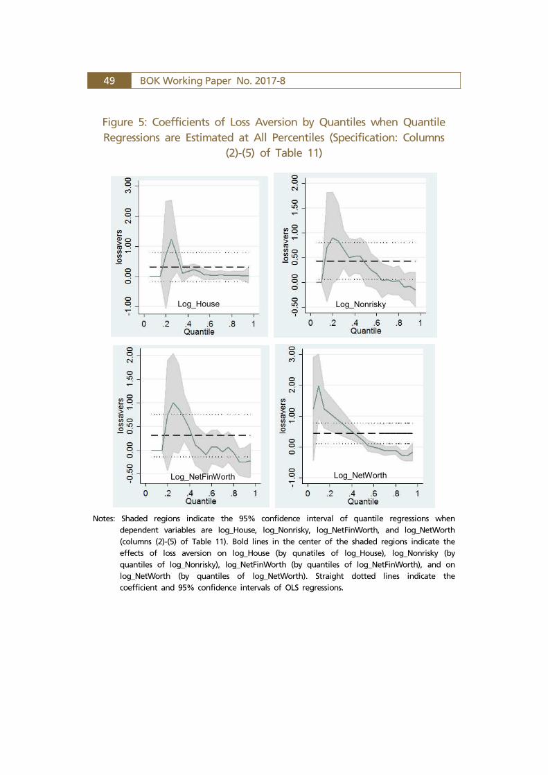
Figure 1: Proportion of Protection and Savings Elements in a Whole Life Insurance Contract Issued at Age 35

Notes: Based on a 35-year-old nonsmoking male with a preferred-rate of a $100,000 whole life insurance policy sold by New York Life Insurance Company. Life expectancy of the person is assumed to be 83.

Data Source: Insure.com (2015), Data retrieved from http://www.insure.com/life-insurance/cash-value.html

http://www.insure.com/life-insurance/cash-value.html


Individual vs. group policy

Group life insurance is a type of life insurance that covers an entire group of

people. Group life insurance is typically offered by an employer or professional

association to its employees or members. The most common type of group life

insurance is employer-provided term-life insurance. Employers pay some or all

of the premiums of term-life insurance as a part of a benefits package. Many

employers limit the coverage of group term-life insurance to $50,000 because

employees are subject to income tax if the coverage of employer-provided

term-life insurance exceeds $50,000 (IRS, 2016).2)

Unlike group life insurance, individual life insurance is purchased, maintained,

and controlled by an individual. Even if the insured change a job, the coverage of

individual policy is not affected by the change unlike the employer-provided

policy. Thus, what is closely related to an individual’s willingness to ensure

themselves is individual life insurance rather than group policies.

2.2 Literature

2.2.1 Determinants of life insurance take-up

Studies by Mossin (1968), Yaari (1965), and Fisher (1973) lay the theoretical

foundation for the determinants of life insurance. These studies point out that

risk aversion, bequest motives, labor income, wealth, and prices (premiums of

insurance, returns of other assets) are determinants of life insurance demand.

Specifically, those who have high risk aversion and strong bequest motives are

more likely to buy life insurance, and those who live by working are more likely

to purchase insurance than those who live off the proceeds of their wealth

(Fisher, 1973).

Despite the theoretical importance of risk aversion in insurance demand,

little empirical evidence is reported on the relation between the measures for

risk-aversion and ownership of life or non-life insurance. Green (1963, 1964)

2) Retrieved from https://www.irs.gov/government-entities/federal-state-local-governments/group-term-life-insurance.


explores the relationship between the two. He measures individuals’ risk

aversion using attitudes toward small and large gambles. He concludes that

there is no correlation between risk aversion and ownership of health, auto, and

life insurance. Similarly, recent studies by Gottlieb and Mitchell (2015) and

Hwang (2016a) find no association between the CRRA measure for risk aversion

and ownership of long-term care insurance, supplemental disability insurance,

or private health insurance. Another line of research attempts to measure the

magnitude of each household’s risk, so-called ‘financial vulnerability’ (e.g.,

volatility of standard of living in case a major income earner of a household is

to die), and investigates its association with insurance ownership. Bernheim,

Carman, Gokhale and Kotlikoff (2003), Bernheim, Forni, Gokhale and Kotlikoff

(2003), and Mountain (2015) find no association between a household’s

financial vulnerability and its life insurance ownership. In contrast, Lin and

Grace (2007) report that households’ financial vulnerability is positively

associated with life insurance ownership.

Rather than using direct measures for risk-aversion, most empirical studies

on insurance purchasing behavior have used demographic variables (e.g., age,

gender, family structure) as a proxy for risk aversion due to a difficulty of

measuring attitudes toward risk. These studies have reported inconsistent and

contradictory results as to which effects (positive vs. negative effects) such

demographic factors have on the take-up of life insurance (Zietz, 2003;

Outreville, 2014). Specifically, Outreville’s (2014) literature survey reports that

“Almost all past research dealing with panel or survey data in the United States

has focused on life insurance purchasing behavior as a function of various

demographic and socioeconomic variables” (p. 170). For example, the literature

has included gender, age, marital status, and education as the proxies for risk

aversion based on the fact that women, elderly, married, and undereducated

individuals are more risk-averse. Regarding the effect of demographic variables

on life insurance, prior studies have reported mixed results. For example,

Outreville’s literature survey summarizes the effects of age on life insurance

holdings as follows: half of the literature reports a positive association of age

with life insurance holdings while the other half reports a negative association.


Some studies report an insignificant relation between age and life insurance

holdings. Similar contradictory findings are reported on the effects of

education, marital status, and family size on life insurance ownership.3)

Several studies associate bequest motives with life insurance take-up.

Bernheim (1991) suggests empirical evidence indicative of strong bequest

motives using income and insurance ownership data on the U.S. elderly.

Bernheim finds that a high level of social security benefits is positively associated

with ownership of life insurance, and concludes that this could be evidence of a

strong bequest motive. The rationale for this conclusion is that individuals buy

life insurance to de-annuitize their wealth because, under strong bequest motives,

individuals can be over-annuitized by government-provided Social Security

annuities. Bernheim’s annuity offset model of life insurance is carefully

examined by Brown (2001) using detailed life insurance ownership data in which

two types of life insurance (term-life vs. whole-life) are distinguishable. Brown

shows empirical evidence to the contrary of the annuity offset model, including

the facts that (i) many individuals own term-life insurance and private annuities

at the same time, and (ii) Social Security benefits are not significantly positively

associated with holdings of term-life insurance.

2.2.2 Behavioral factors and insurance buying decisions

A growing body of research has begun to explore the effects of behavioral

tendencies on insurance purchasing decisions. However, to my knowledge, no

empirical evidence is provided for the life insurance market. An earlier study by

Johnson et al. (1993) shows that availability heuristics and framing effects are

associated with individuals’ willingness to pay for insurance (flight, auto, and

3) These inconsistencies in empirical studies seem to be associated with the possibility that demographics variables affect insurance holdings through multiple channels. For example, gender affects insurance holdings directly or indirectly through its association with risk aversion. Specifically, being female means that the person is less likely to be a major income earner of a household; hence, females are less likely to demand life insurance (direct impact). But in terms of risk aversion, females are more risk averse than males; hence, women may have a higher willingness to pay for insurance (indirect impact through risk-aversion).


disability insurance). For example, the study shows that consumers express a

higher willingness to pay for insurance when the relevant accident comes across

their mind readily and vividly (availability heuristics). It also shows that

consumers tend to prefer expensive return-of-premium insurance to much

cheaper insurance that returns a lower amount of money, which is actuarially

better (framing effect: guarantee or rebate frames are preferred). An

experimental study by Brown, Kling, Mullainathan, and Wrobel (2008) also

reports a similar framing effect: people’s willingness to pay for annuities is

affected by the way annuity products are described, i.e., the

insurance-on-consumption frame vs. the investment frame. Only recently have

researchers begun to relate behavioral factors to real-world insurance holdings

data beyond the laboratory settings. (for reviews, refer to Camerer (2004) and

Barberis (2013)). Gottlieb and Mitchell (2015) show that narrow framing, as

measured by an indicator variable for whether a respondent changes his

decision when problems are presented within a negative frame, is negatively

associated with ownership of long-term care insurance using the HRS data set.

Bhargava, Loewenstein, and Sydnor (2015) analyze health insurance choices of

workers at large firms and find that their choices are subject to heuristics.

Hwang (2016a) focuses on the role of loss aversion and shows that loss aversion,

as measured by the amount of acceptable losses in small-amount gambles, is

negatively associated with the holdings of long-term care insurance,

supplemental disability insurance, and private health insurance using the

American Life Panel data. Hwang points out that the majority of prior studies

have neglected to consider the role of loss aversion in insurance take-up

because most prospect-theory-based studies have assumed that individuals

assess insurance products entirely within the “loss domain”, not within both the

gain and loss domain as Hwang assumes (pp. 3-4, 38-30).


Ⅲ. Model: Loss Aversion, Term-life Insurance, and Saving

3.1 Background: prospect theory’s loss aversion & insurance

Loss aversion means people’s tendency to be more sensitive to losses than

the same amount of gains. This is one of the most important features of

Kahneman and Tversky’s (1979, 1992) prospect theory. Prospect theory states

that people decide whether to buy a prospect or a lottery based on the expected

value of potential gains and losses from the reference point. More formally,

prospect theory states that the gain-loss value from a prospect is ,

where ․ is the probability weighting function, is the probability of possible

outcomes, ․ is the value function, and is a random variable representing

losses or gains from the prospect. Kahneman and Tversky specify the value

function as ≥

, where is the coefficient of loss

aversion. Figure 3 (b) illustrates the value function. According to prospect

theory, whether to participate in a lottery depends on several parameters, such

as the degree of loss aversion (), reference point (this determines gains or

losses, ), probability weighting (․), and the degree of diminishing

sensitivity ( , ). Kahneman and Tversky (1992) have found that, in their

laboratory experiments, most people exhibit a greater than one. Kahneman

and Tversky estimate .

This paper focuses on the role of loss aversion when a particular reference

point is adopted. It also examines how loss aversion interacts with the expected

survival probability. This paper, however, does not focus on the role of diminishing

sensitivity because this paper assumes that insurance is evaluated in both the gain

and loss domains as in Hwang (2016a), where and play little role.

If people assess the value of insurance as they access the gain-loss value of a

lottery, then the value of insurance is negatively associated with the degree of

loss aversion, . Hence, loss-averse individuals may be less likely to purchase

insurance. Specifically, the expected gain-loss value of a prospect, E[], is

negatively associated with the degree of loss aversion . To see this, suppose the


probability of gain from a prospect is and the probability of loss from the

prospect is . Furthermore, assume for simpliticy. In this case, the

expected value of the prospect is . Hence, the

value from a prospect is negatively associated with the degree of loss aversion.

The two underlying assumptions in deriving the result are as follows: first,

people have narrow framing (i.e., people isolate risk) in the sense that they only

care about the gain-loss value of a prospect, not about the diversification effect

that the prospect will bring to their existing portfolio; second, the reference

point is “the wealth level when one does not engaging in the prospect,” which

means that no gains or no loss occurs if a person does not take action for buying

insurance (See Proposition 1 of Hwang (2016a)). One can also see that loss

aversion interacts with ‘ ’ (i.e. ). This implies that

the effect of loss aversion is large among those who believe that an accident will

not occur.

To exemplify the effect of loss aversion, consider a lottery that has 50-50

chances of winning $200 or losing $100. Further assume that a person has a

preference with . One can show that whether this person

will accept or turn down the lottery depends on the person’s degree of loss

aversion (). For example, if the person has a of three, the person will turn

down the lottery because the gain-loss value of the lottery is negative

(0.5*$2001-0.5*3.0*$1001=-$50). If the person has a of 1.5, then the person

will accept the lottery because the gain-loss value becomes positive.

(0.5*$2001-0.5*1.5*$1001 = +$25).

3.2 Model

This paper considers the effect of loss aversion on life insurance take-up and

savings within the context of Dynan, Skinner and Zeldes’ (2002; 2004) life

cycle/permanent income model with a bequest motive. In this model,

individuals face uncertainties regarding future earnings and the length of life.

There are three periods in the model (, , and ). Figure 2 illustrates

the 3-period model of uncertain lifetimes.


Individuals are alive for sure at , but it is uncertain whether they will survive

at . Those who survive at die for sure at . One can think of period

(“young”) as ages 30-60, period (“old”) as ages 60-90, and period

as the time around death, as Dynan et al. point out (2004, p. 403). The two

possible states of the second period are notated as . If is

realized, then the person dies at the beginning of . If is realized, then

the person survives at (and dies at ). The amount of bequests he/she

leaves in the event of death at the beginning of and is Q and

Q respectively. Individuals’ subjective probability of experiencing and

is and respectively, where . Faced by uncertain lifetimes, in the

first period (), an individual decides how much to consume, save, and buy

term-life insurance. If the individual is alive in the second period ( ), the

person decides how much to consume for himself/herself and set aside for

inheritance.

Most previous studies, including Dynan et al. (2002; 2004), assume a perfectly rational consumer and use the following preference specification: a

Figure 2: Three Period Model of Uncertain Lifetimes

Source: Author's illustration


consumer maximizes expected lifetime utility coming from consumptions (C ,

C ) and bequests (Q , Q ):

(2.1) ․ ․ ․

D is an indicator variable that is equal to one if (death) is realized and

zero otherwise. U(․) and G(․) represent utility functions for consumptions and

bequests. is a discount factor (0≤≤1) .

This paper extends the domain of preference: it assumes a boundedly rational consumer who gets utility not only from consumptions and bequests

but also from the “gain-loss” utility of risky assets, following the prospect theory

literature (e.g., Barberis, Huang, and Santos, 2001; Hwang, 2016a). A

boundedly rational consumer maximizes the following expected utility:

(2.2) ∗ ․ ․ ․

(2.3) ≥

(2.4)

(2.5)

, , ∈

The term represents the gain-loss value of insurance, where ․ is

Kahneman and Tversky’s (1979) value function and is the quantity of

term-life insurance.4) One important parameter of the value function is , a

coefficient of loss aversion (See 2.3). The utility function for consumptions and

bequests is assumed to be the CRRA utility function, which has a risk aversion

parameter (See equations (2.4-2.5)). As a result, the insurance-savings model

in this paper incorporates both the risk aversion measure () and the loss

aversion measure ().

Table 1 and Figure 3 compare the risk aversion measure with the loss

aversion measure. While loss aversion decreases insurance demand, risk

aversion increases insurance demand. If the negative effect of loss aversion on

insurance demand is dominated by the positive effect of risk aversion, then a

4) The term can be re-written by ∗ ∗∗ .


person decides to buy insurance. (i.e., even though a person has a high

magnitude of , he/she may be willing to buy insurance if is large)

The term is a scaling factor that reflects the degree of narrow framing or

intuitive judgment. A high magnitude of indicates that an individual’s

decision is significantly affected by the gain-loss value, which is in turn

determined by . If is zero, then this implies that a person’s decision is not

affected by but determined solely by the CRRA parameter . Note that a

boundedly rational consumer’s utility in (2.2) includes the fully rational

consumer’s utility in (2.1). Specifically, a perfectly rational consumer’s objective

function (2.1) is a particular case of a boundedly rational consumer’s objective

function (2.2) where is zero. In this regard, this paper deals with a more

generalized problem.

Table 1: Comparison between the Risk Aversion Measure and the Loss Aversion Measure

Risk Aversion: CRRA measure (γ) Loss Aversion (λ)

Domain γmeasures the concavity of Bernoulli’s utility function, which is defined over final wealth (or consumption)

λmeasures the concavity of Kahneman and Tversky’s value function defined over gain and loss

Example of a survey question

Large amount gamble question (Barsky et al., 1997):(e.g.) Would you take a new job that has a 50-50 chance of doubling your total lifetime income or cutting it by a third?

Small amount gamble question (Kahneman and Tversky, 1992):(e.g.) Would you agree to an investment that has a 50-50 chance of receiving $200 or paying $100?

Features Attitude to risk under the deliberation mode (system 2) orattitude to risk in a comprehensively inclusive context

Attitude to loss under the intuition mode (system 1) orattitude to loss when correlations are neglected (narrow framing)

Effect on insurance

γ↑è Insurance demand ↑ λ↑è Insurance demand ↓

Key theory Expected utility theory Prospect theoryNarrow framing

Agent in consideration

Perfectly rational agent Boundedly rational agent

Notes: The insurance-savings model in this paper incorporates both γand λ. The relative importance of the two parameters on decision making is determined by a scaling factor .


The term in (2.5) is the weighting function for bequests, which is

commonly used in the related literature (e.g., Fischer, 1973). If is one, this

indicates that an individual attains the same level of utility from bequests as

consumptions. A of zero indicates that an individual does not value bequests.

Two assets are available in the economy in the first period: single-period

term-life insurance and a riskless bond. The term – or more precisely,

– represents the quantity of the single-period term-life

insurance that pays out units of consumption at if and only if is

realized. The term – or more precisely, – is the unit price of

the term-life insurance. For example, if and , this means

that a person abandons one unit of period t consumption (1=0.5*2) in order for

his/her heirs to receive two units of period consumption if is realized.

The quantity of a riskless bond is denoted by (written in terms of the period

consumption good). A positive value of means saving. No non-negativity

Figure 3: Two Measures for Attitude toward Risk-or-loss in the Model

Notes: While the CRRA risk aversion measure () captures the concavity of Bernoulli’s utility function (left), the loss aversion measure () captures the concavity of Kahneman and Tversky’s value function (right). The model in this paper incorporates both and λ.

Source: Hwang (2016a)


restrictions are imposed on or . (Note that having negative

holdings of is analogous to buying annuities). There is, however, perfect

enforcement of financial contracts. This asset market is complete because

consumers can re-allocate resources across different states and periods by buying

and selling and .5) Earnings at are denoted by .

Consumers’ budget constraints are as follows: 6)

(2.6) ․ ≤

(2.7) ≤ ․

(2.8) ≤ ․

The units in all constraints are the consumption good.7) The budget

constraint (2.6) illustrates that an individual decides how much to consume, buy

term-life insurance, or buy riskless bonds, given the earnings in the first period.

Inequalities (2.7) and (2.8) illustrate the constraints in the second period. If a

person dies (i.e., ), then all of his/her assets become the bequests

( ). The assets include earnings ( , e.g., Social Security

survivors benefits), death benefits of term-life insurance ( ), and the

principal and interests of bonds ( ․ ). Inequality (2.8) illustrates the case

where a person survives at ( ): the person decides how much

to consume ( ) and how much to set aside for bequests ( ).

A boundedly rational consumer’s problem is as follows:

(2.9) Given prices , max

subject to (2.6), (2.7), (2.8), ≥0, ≥0, ≥0, and ≥0

5) The introduction of another type of insurance to the economy, for example , does not change the

oplimal level of consumption or bequests.6) Budget constraints hold with equality as strictly monotonic utility functions are assumed.7) Note that if we assume an infinitely lived household without bequest motives, the budget constraint (2.6),

(2.7) & (2.8) can be generalized as follows: ∈

․

≤

․

The above constraint is the standard budget constraint when sequential markets and uncertainties are considered, except for the case that a redundant asset, , (which is the same as purchasing arrow securities for all possible states) is added. A similar budget constraint can be found in Dirk Kruger’s macroeconomics textbook (p. 101 of “Macroeconomic Theory”).


The Lagrangian and the first order conditions (FOC) for interior solutions

are as follows:8)

(2.10) ∗

․ ․

․

․

․

․

(2.11) ′) =

(2.12) ′ =

(2.13) ′ =

(2.14) ′ =

(2.15) ∗′ =

(2.16)

=

The above FOCs can be summarized as follows:

(2.17) ′ ∗′ =

′

(2.18)

′

= ′

′

(2.19)

′

= ′

′

The intertemporal budget constraint summarizing (2.6), (2.7), and (2.8) is as

follows:

(2.20) ․

= ․

․

Optimal levels of saving and term-life insurance for perfectly rational agents (, )

By plugging the FOCs into (2.20), one can get optimal levels of consumption,

bequests, and assets. We first look at a perfectly rational consumer’s optimal

choice by setting .

8) Since CRRA utility function satisfies inada conditions, C* > 0. And since CRRA with > 0 is strictly concave, FOCs guarantee unique global max.


(2.21)

․

(2.22)

․

(2.23)

․

(2.24)

․

(2.25)

․｛

｝․

(2.26)

․

․

․

․

Mossin’s (1968) Theorem and Yaari’s (1965) result

Equation (2.25) shows a perfectly rational consumer’s optimal level of

term-life insurance. Note that if (i) premiums of term-life insurance are fair

( ; here, it is also assumed that a subjective probability of survival is the

same as the objective probability), (ii) a bequest motive is sufficient to be , and (iii) the price motive for saving is neutral (i.e., ․ ),

then Mossin’s (1968) result holds: risk-averse individuals fully insure themselves

if premiums are fair. Under such conditions, the optimal quantities of insurance

and bond are

and

․ ․

. This leads to an allocation

.

If we assume that there is no bequest motive ( ), while keeping

the assumptions (i) & (iii), then Yaari’s (1965) full annuitization result holds:

risk-averse individuals with no bequest motive fully annuitize their assets.

Under these assumptions, the optimal quantities of insurance and bond are

and

․ .9)

This leads to an allocation of and

and

,


which means a full annuitization.

Although this three-period model of saving and term-life insurance is

simple, it enables the analysis of various aspects of term-life insurance and

saving ( ):

① life cycle / permanent income motives for saving;

② precautionary motives for saving (Skinner, 1987);

③ the effect of a bequest motive on life insurance and saving;

④ the effect of loss aversion on life insurance and saving;

This paper focuses on “④ the effect of loss aversion on life insurance and

saving” while considering ①-③.

Introduction of whole-life insurance

Whole-life insurance serves as a saving instrument as well as insurance:

whole-life insurance accumulates cash value, and consumers can withdraw

money based on the reserved fund of the insurance policy (savings feature);

furthermore, whole-life insurance pays out death benefits if the insured die

(insurance feature). In the three-period model, purchasing whole-life insurance

is the same as simultaneously purchasing term-life insurance and riskless bonds

( ). Formally, one can imagine units of whole-life insurance that can be

purchased at t. Assume that the cash value of this insurance becomes ․ at

and ․ at . If the insured die at (i.e., ), then the

insurance pays out death benefits of ․ . If the insured die at (i.e.,

), then the whole-life insurance pays out ․ units of

consumption as death benefits. In this case, purchasing units of whole-life

insurance is the same as purchasing the same units of riskless bonds and

purchasing ․ units of term-life insurance.

9) Note that >

.


3.3 Testable implications of the model

[A1] Increase in loss aversion () decreases the demand for term-life insurance ( )

A1 holds because loss aversion creates a negative gain-loss utility whenever

an individual purchases term-life insurance. Hence loss aversion decreases the

demand for term life insurance, .

FOCs show this prediction more clearly. Plugging (2.17) into (2.18) and

(2.19) leads to the following equations:

(2.27)

′

′

′

(2.28)

′

′

′

To figure out how loss aversion affects ′ , we first look at

which is the expected gain-loss value when purchasing

units of term-life insurance. A potential gain of the insurance is the

present value of the net benefits from the insurance company

. The gain is realized if . A potential loss of

the insurance is the premium paid . The loss is realized if

Hence, the expected gain-loss value is as follows:

(2.29)

․ ․

Thus, if we take derivatives with respect to , then we have

(2.30) ′

Hence, an increase in decreases the marginal gain-loss value (left-hand-side

(LHS) of (27)). To keep the equality, the right-hand-side (RHS) of (2.27) must

decrease. This means that ′ should increase relative to

′ . (Note that

is a positive value). To increase the

marginal utility of a bequest in the case of death at relative to

that of consumption in the case of survival , the level of bequest


should decrease relative to the consumption . Similarly,

equation (2.28) implies that the level of a bequest at , should

decrease relative to the level of a bequest at . Budget

constraints (2.7) and (2.8) imply that decreasing relative to

and can be attained by decreasing term-life insurance. That is, the

transfer of resources from state to state can be accomplished by reducing

term-life insurance holdings.

[A2] An increase in loss aversion () increases savings ( )

This means that loss-averse individuals save more in order to use savings as a

financial buffer against potential bad events in the future instead of using

term-life insurance as a financial buffer. FOC (2.18) provides the rationale for this.

Equation (2.18) implies that marginal cost of giving up today’s consumption

should be the same as the expected marginal benefits of tomorrow’s bequest

and consumption. Suppose decreases or becomes zero because of a

high loss-aversion. This leads to an increase in today’s consumption ( ) and a

decrease in the bequest for . Hence, the LHS of (2.18) decreases,

while the first term in the RHS increases. To maintain equality, the second term

in the RHS (the marginal utility of tomorrow’s consumption) should decrease.

Hence, the level of tomorrow’s consumption, , should increase. This is

done by increasing savings ( ). Similar logic applies to the FOC (2.19) and

leads to the same conclusion.

[A3] Loss aversion has less impact on the take-up of whole-life insurance than

on term-life insurance.

This is because whole-life insurance serves as a saving instrument as well.

Even if is realized, the insured can still withdraw money based on the

reserved fund of the whole-life insurance policy. Hence, the potential loss from

whole-life insurance is smaller than that from term-life insurance.


[A4] The weights for bequests ( , ) have different impacts on term-life

insurance and saving. An increase in increases the demand for term-life

insurance, while it decreases the demand for saving ( ). In contrast, an

increase in decreases the demand for term-life insurance, while it increases

the demand for saving ( ).

The weight, represents the desire for leaving bequests in the event of an

unexpected premature death ( ), while represents the desire for leaving

bequests for an expected death at a later time.

An increase in increases the demand for term-life insurance, while it

decreases the demand for saving ( ). This is because a transfer of resources

to the state of premature death () is made by term-life insurance. A formal proof is provided in Appendix B.

In contrast, an increase in decreases the demand for term-life

insurance, while it increases the demand for saving ( ). This is because a

transfer of resources to state can be attained by reducing term-life insurance and increasing savings.

[A5] The effect of loss aversion on the demand for term-life insurance is

amplified by the degree of narrow framing ( ) and the expected survival

probability ().

Equation (2.30) shows this prediction clearly. Since the scaling factor, , determines the degree to which the gain-loss value affects individuals’ decisions,

a high magnitude of implies a high impact of loss aversion () on insurance take-up. And since the potential loss is associated with , the subjective

probability of experiencing () affects the impacts of loss aversion.


Ⅳ. Empirical Tests Using the Health and Retirement Study

4.1 Loss aversion data

The degree of loss aversion, which is formally defined by , captures

the relative sensitivity to losses compared with the same amount of gains.

Kahneman and Tversky (1992) measure loss aversion using small-amount risky

gamble questions (e.g., accept or turn down a prospect that has a 50-50 chance

of losing $100 or winning $202).10) This paper uses a similar question.

This paper uses the Health and Retirement Study (HRS) Public Data. The

HRS is a longitudinal panel survey that interviews a representative sample of

approximately 20,000 Americans over the age of 50 every two years (HRS

webpage). While regularly collecting detailed information on respondents’

assets and health status, the HRS also conducts a one-time survey on special

topics called an ‘experimental module’ (experimental modules are also publicly

available). Survey questions about respondents’ attitudes toward small-amount

risky investments are included in the Prospect Theory Module of the 2012

HRS. Details of the Prospect Theory Module are explained in the principal

investigators’ study on narrow framing and long-term care insurance (Gottlieb

and Mitchell, 2015). Specifically, this paper uses the following questions, which

are randomly assigned to about 1,900 HRS respondents: 11)

“Suppose that a relative offers you an investment opportunity for which

there is a 50-50 chance you would receive [$103 or have to pay $100].

10) The theoretical foundation of the loss aversion measure is discussed in Rabin (2000), Rabin and Thaler (2001), and Barberis, Huang and Thaler (2006). These studies prove that subjects’ behavior of turning down a small favorable prospect cannot be rationalized without introducing subjects’ neglect of the diversification effect that the prospect may bring. In the HRS sample, approximately 94.4% of respondents turn down the Receive-$103-or-Pay-$100 investment, suggesting that they tend to neglect correlation. Hence, for at least 94.4% of respondents, the small-amount-risky-investment-questions in this paper capture how individuals assess gain and loss when correlations are neglected. This feature allows the questions to measure loss aversion as defined by Kahneman and Tversky (1992).

11) Technically, not all seven questions are asked to respondents. All respondents are first asked ‘(4) Receive $115 or pay $100’ question. If a respondent agrees to this investment, then, ‘(2) Receive $107 or pay $100’ is asked. If a respondent does not agree to the initial question (4), then ‘(6) Receive $130 or pay $100’ is asked. Similar rules are applied to the subsequent questions. For details, see Gottlieb and Mitchell (2015).


Would you agree to this investment?

(1) Receive $103 or pay $100 (2) Receive $107 or pay $100



(7) Receive $300 or pay $100”

Among the selected sample of 1,900 elderly people, 1,698 complete the

survey. Table 2 shows the results. Nineteen percent of the respondents reject

investments (1)-(6) but accept the investment (7), indicating that their loss

aversion is greater than 1.3 and equal to or less than 3.0. For these individuals,

loss aversion of 2.15 (average of 1.3 and 3.0) is assigned. Approximately two

thirds of the respondents reject all seven risky investments, indicating that their

loss aversion is greater than 3.0. As a result, the median of is estimated to be

higher than three, which is higher than Kahneman and Tversky’s estimation

result (median of = 2.25). It seems that this high loss aversion is associated

with the sample of the HRS, which only surveys the elderly (aged 51 or more),

who, in general, have a more conservative attitude toward loss than the young.

Table A.4 (Appendix) presents the degree of loss aversion by demographics.

Although there is no statistical significance, females, those aged 70 or older, less

Table 2: Estimation Results of Loss Aversion ()

Risky InvestmentsThose who accept the

investment but rejects other less favorable investment offers

Range of Implied

Loss Aversion

SelectedLoss Aversion

　 N (percent)

(1) Receive $103 or pay $100 95 (5.6) ≤1.03 1.015

(2) Receive $107 or pay $100 22 (1.3) 1.03≤1.07 1.05

(3) Receive $110 or pay $100 5 (0.3) 1.07≤1.10 1.085

(4) Receive $115 or pay $100 66 (3.9) 1.10≤1.15 1.125

(5) Receive $120 or pay $100 24 (1.4) 1.15≤1.20 1.175

(6) Receive $130 or pay $100 24 (1.4) 1.20≤1.30 1.25

(7) Receive $300 or pay $100 323 (19.0) 1.30≤3.00 2.15

Reject 'Receive $300 or pay $100' 1,139 (67.1) 3.00 3.15

Total 1,698 (100.0) - -

Source: HRS 2012, Prospect Theory Module


educated people, and those with fewer children tend to be more loss-averse.

Risk aversion, which is based on the status-quo-bias-free lifetime income gamble

questions (Barsky et al., 1997), shows a similar pattern.

4.2 Life insurance ownership and wealth data

Detailed information on the definitions, sources, and characteristics of the

data is reported in Table A.1-A.3 (Appendix). Life insurance ownership

information is based on the following questions from the 2012 HRS

(N=18,712):

(i) “Do you have any life insurance, including individual or group policies?

IWER: Do not include burial insurance.” (HRS code: NT011)

(ii) “How many different life insurance policies do you have?

IWER: Include individual policies, group policies, or paid-up policies if R

asks.” (NT012)

(iii) “[What/Altogether, what] is the total face value of [this policy/these

policies], that is, the amount of money the beneficiary would get if you were

to die?” (NT013)

The HRS also collects ownership information about whole-life insurance.

(iv) “[Is this a life insurance policy that builds/Are any of these life insurance

policies ones that build] up a cash value that you can borrow against, or that

you would receive if the policy were to be cancelled?

Def: (These are sometimes called 'Whole Life' or 'Straight Life Policies.')”

(NT018)

(v) “How many such policies do you have?” (NT019)

(vi) “What is the current face value of [these policies/this policy]?” (NT020)

Since the 2012 HRS does not survey the ownership of term-life insurance,

we estimate term-life insurance ownership information based on the fact that

life insurance is either term-life or whole-life insurance. For example, suppose a


respondent answers that he/she has two life insurance plans, and their total face

value is $20,000. If the person answers that he/she has one whole-life insurance

plan whose face value is $12,000, then the person is assumed to have one

term-life insurance plan whose face value is $8,000.

To examine if the estimated ownership data on term-life insurance is

reasonable, the estimated data is compared with a data set based on real

interviews on term-life insurance holdings. The 1993 HRS (AHEAD survey)

interviews those aged 70 or older about ownership of term-life insurance (for

details, see Brown 2001). The questions on ownership of term-life insurance are

discontinued after the 1993 survey. Although there is a considerable time gap

between the two surveys (2012 vs.1993), given the scarcity of individual-level

term-life insurance ownership data, this is one feasible way to assess if our

estimated data is reasonable. In the 1993 HRS, the ownership rate of term-life

insurance among married men and women aged 70 and older is 41.74 and

30.14 percent respectively. In the 2012 HRS, the estimated ownership rate of

term-life insurance among married men and women aged 70 and older is 37.51

and 26.09 percent respectively. Considering the time gap, it seems that the

difference falls within an acceptable range. Both data show that roughly one

third of those aged 70 or older own term-life insurance, indicating that many

U.S. elderly utilize the renewal option of term-life insurance.12)

In the 2012 HRS data as a whole (aged 51 and older), 56.0 percent of

people are found to hold life insurance: 38.0 percent own term-life insurance

and 25.4 percent own whole-life insurance. Among them, 7.4 percent own both

term-life and whole-life insurance (see Table 3). The median of the total face

value conditional on owning any life insurance is $45,000, and the conditional

average of the total face value is $116,105. Life insurance owners have on

average 1.54 life insurance plans. In the case of term life insurance, the median

12) Considering that one primary goal of life insurance is to protect family against the loss of a primary wage earner, which is especially true in the case of term-life insurance, the elderly’s owning of (term-) life insurance raises questions regarding their motives since most elderly people do not earn wage income. Regarding this question, Brown (2001) has discussed various reasons: (1) protection of the spouse against loss of pension or Social Security income, (2) residue from a past attempt during working-age to protect human capital, (3) tax planning, and (4) covering funeral expenses (p. 117).


of the total face value conditional on holding any term-life plan is $50,000, and

the conditional average of the total face value is $124,589.

Detailed ownership information in Table A.5 (Appendix) shows that wealthy,

highly-educated, male, and married individuals, as well as those with children,

are more likely to hold a life insurance policy.

One important limitation of the HRS data is that it does not distinguish if a

respondent’s life insurance policy is an individual policy or a group policy.

Since many employers provide term-life insurance as a part of a workplace

benefits package, this limitation could be a confounding factor in investigating

how individual’s behavioral tendencies affect insurance buying decisions. To

alleviate this issue, we take the following approaches. First, the analysis is

restricted to those aged 60 or older in all regressions, so that our samples are

less affected by the employer-provided term-life policies, which are tied to

employment (of those aged 60 or older in the HRS sample, only 20.26 percent

are employed). Second, an indicator variable is added to determine whether the

respondent is currently working in all regressions. Third, for the robustness

check, occupation dummies (to the respondent’s job with the longest reported

tenure13)) are added. Fourth, whether or not loss aversion is associated with the

probability of “holding two or more plans of term-life insurance” and with the

13) Employer-provided term-life insurance has a renewal option, which means that those who retire may keep term-life coverage if they decide to pay premiums by themselves. Hence, retirees’ term-life ownership can be affected by past employment history. Control for the past occupation history can alleviate this issue.

Table 3: Life Insurance Ownership of the U.S. Elderly in 2012 (Age≥51)

　 Any life insurance Term-life Whole-life

Ownership rate (own=1) 0.560 0.380 0.254　　　　

Amount | Own 　　　

Medican ($) $45,000 $50,000 $30,000

Mean ($) $116,105 $124,589 $75,005　　　　

Average number of plans | Own 1.54 1.37 1.33

Note: Unweighted data.Source: HRS 2012


amount of “face value $50,000” is tested based on the fact that employer-provided

term-life policies are typically limited to one plan with a face value of $50,000.

Five variables are used for household wealth levels in 2012: Stock, House,

Nonrisky, Net Fin Worth, and Net Worth. The source of these wealth variables is

the RAND HRS Income and Wealth Imputations-Version O (March 2016). Stock

is the net value of stocks, mutual funds, and investment trusts that a household

owns (RAND HRS code: H11WSTCK). House is a net value of primary

residence (H11WTOTH). Nonrisky is the sum of the ‘value of checking,

savings, or money market accounts,’ ‘value of CDs, government savings bonds,

and T-bills,’ and the ‘net value of bonds and bond funds.’

(H11WCHCK+H11WCD+H11WBOND). Net Fin Worth is the net value of

non-housing financial wealth (H11WTOTN = Stock + Nonrisky + net value of

all other saving value of other debt (other than mortgages, land loans, or

home loans)). Net Worth is total net wealth including secondary residences

(H11WTOTB = Net Fin Worth + House + Net Value of Secondary Residence).

Table 4 reports five wealth variables by age group. One important pattern to

note is that elderly households increase their wealth level even after retirement

(so called savings puzzle): those aged 70-79 have a higher net worth level than

those aged 60-69; those aged 80-89 have an even higher net worth level. This

Table 4: Median Levels of Household Wealth by Age Group in 2012 (Nominal Dollars)

　(Number of Households)

Age 51-59(3,732)

60-69(3,095)

70-79(3,048)

80-89(1,503)

90-99(413)

Stock 0 0 0 0 0

House 20,000 60,000 80,000 79,000 0

Nonrisky 1,000 2,500 5,000 10,000 6,000

Net Fin Worth 0 2,000 7,975 18,450 10,000

Net Worth 50,000 111,500 160,000 173,800 79,000

Note: Unweighted cross-section data in 2012. Nonrisky = value of checking, savings, or money market accounts + value of CDs, government

savings bonds, & T-bills + net value of bonds and bond funds. Net Fin Worth = Stock + Nonrisky + net value of all other saving value of other debt (other

than mortgages, land loans, or home loans). Net Worth = Net Fin Worth + House + Net Value of Secondary Residence.Source: RAND HRS Income and Wealth Imputations-version O (March 2016)


wealth accumulation pattern is not consistent with the predictions of the

permanent income / life cycle model of saving, which predicts a substantial

dissaving after retirement.

4.3 Loss aversion and term-life insurance & whole-life insurance

4.3.1 Descriptive statistics

To control for employer-provided term-life insurance and the life cycle effect of

saving, we restrict our sample to those 60 and older. When one uses all samples of

the HRS (i.e., those 51 and older), however, one can also find a similar empirical

result, i.e., a negative association between loss aversion and the take-up of term-life

insurance as reported in Table A.6 (Appendix).

Panel A of Table 5 shows that loss aversion is significantly negatively correlated

with the term-life insurance holdings and positively correlated with the household’s

wealth. These results are consistent with the prediction [A1]-[A2] in the previous

section. Specifically, the high loss-aversion group shows a significantly lower

ownership rate of term-life insurance than the low loss-aversion group (34.2% vs. 41.5%). In terms of both the number of term-life insurance policies (0.448 vs. 0.573) and the total coverage amount of term-life insurance (logged value: 2.950 vs. 4.031), the high loss-aversion group has significantly lower figures. In contrast,

being highly loss averse or not does not show a statistically significant association

with whole-life insurance, which is a combination of insurance and savings. If we

look at the pure savings side, Net Financial Worth and Net Worth are positively

correlated with loss aversion. This is consistent with the model, which predicts that

loss aversion may increase precautionary saving. Figure 4 illustrates main results.

Except for gender, there is no measurable difference in demographics between

the low loss-aversion and high loss-aversion groups in terms of cognitive ability,

education, marital status, and the number of children.

Panel B of Table 5 reports ownership information for term-life and whole-life

insurance, conditional on owning any type of life insurance. Loss aversion is

significantly negatively correlated with term-life insurance holdings and weakly

positively correlated with whole-life insurance.


Figure 4: Loss Aversion, Ownership of Term-life & Whole-life Insurance, and Wealth (Age≥60)

a. Own Term-life Insurance b. Own Whole-life Insurance c. Log Net Worth

Notes: Figure a [b] illustrates the ownership rate of term-life insurance [whole-life insurance] among the low loss aversion group (≤2.15, N=303) and the high loss aversion group (=3.15, N=792). Figure c illustrates the average of Log Net Worth among the low loss aversion group (≤2.15) and the high loss aversion group (=3.15). The error bars indicate the standard errors in Table 5. The high loss-aversion group shows a significantly lower ownership rate of term-life insurance (=pure insurance) than the low loss-aversion group (34.2% vs. 41.5%). The high loss-aversion group shows a weakly higher ownership rate of whole-life insurance (= partial insurance + partial savings) than the low loss-aversion group (27.2% vs. 25.1%). The high loss-aversion group holds a significantly higher level of net worth (=savings) than the low loss-aversion group (logged value 11.002 vs 10.478). These results are consistent with the prediction that loss aversion depresses insurance demand and stimulates savings.


Table 5: Loss Aversion, Term-life and Whole-life Insurance, and Wealth (Age≥60)

Panel A. HRS sample aged 60 or more

　 Those with lowloss aversion (λ≤2.15)

Those with high loss aversion (λ=3.15)

Two tailed t-test forequal mean

　 N=303 N=792 p-valueown_life 0.594 (0.028) 0.563 (0.018) 0.3553num_life 0.917 (0.057) 0.828 (0.034) 0.1723log_amt_life 5.916 (0.312) 5.198 (0.192) 0.0475**own_term 0.415 (0.029) 0.342 (0.017) 0.0275**num_term 0.573 (0.047) 0.448 (0.026) 0.0153**log_amt_term 4.031 (0.311) 2.950 (0.176) 0.0016***own_whole 0.251 (0.025) 0.272 (0.016) 0.5018num_whole 0.323 (0.037) 0.358 (0.025) 0.4442log_amt_whole 1.144 (0.210) 1.031 (0.123) 0.6333　　　　　　log_Stock 2.752 (0.285) 2.525 (0.170) 0.4856log_House 8.398 (0.297) 8.684 (0.183) 0.4117log_Nonrisky 7.095 (0.256) 7.535 (0.149) 0.126log_Net Fin Worth 6.841 (0.305) 7.483 (0.177) 0.0616*log_Net Worth 10.478 (0.245) 11.002 (0.134) 0.0475**　　　　　　cognitive 518.0 (2.07) 516.2 (1.33) 0.4623edu 12.78 (0.187) 12.58 (0.105) 0.3251married 0.561 (0.028) 0.575 (0.018) 0.6708female 0.534 (0.029) 0.610 (0.017) 0.0225**kids 3.302 (0.118) 3.224 (0.074) 0.5790

Panel B. Samples are restricted to those who own any type of life insurance (Age≥60)

　 Those with lowloss aversion (λ≤2.15)

Those with high loss aversion (λ=3.15)


　 N=171 N=411 p-valueown_term|Own life 0.713 (0.035) 0.630 (0.024) 0.0544*num_term|Own life 0.988 (0.065) 0.825 (0.040) 0.0301**log_amt_term|Own life 7.209 (0.402) 5.770 (0.271) 0.0035***own_whole|Own life 0.433 (0.038) 0.501 (0.025) 0.1326num_whole|Own life 0.556 (0.057) 0.662 (0.040) 0.1391log_amt_whole|Own life 2.278 (0.394) 2.358 (0.260) 0.8646

Notes: The values are the average of each group. Standard errors in parentheses. *** p<0.01, ** p<0.05, * p<0.1. own_life (own_term, own_whole) is an indicator variable if a respondent owns any life insurance (term-life insurance, whole-life insurance). num_life (num_term, num_whole) is the number of any life insurance (term-life insurance, whole-life insurance) a respondent holds. log_amt_life (log_amt_term, log_amt_whole) is the natural log of 'the face value of life insurance (term-life insurance or whole life insurance) + 1'. cognitive is a respondent's total score on the quantitative number series of the HRS. edu is years of education. log_Stock (log_House, log_Nonrisky, log_NetFinWorth, log_NetWorth) is the natural log of 'Stock (House, Nonrisky, NetFinWorth, NetWorth) +1' (The value in the log is replaced with one if the original value is less than one).

Sources: 2012 HRS, RAND HRS Income and Wealth Imputations-Version O (March 2016)


4.3.2 Regression results 1: loss aversion, term-life and whole-life insurance

Our estimating equations are as follows:

1(insurance) = …………… Probit Model

Number_of_insu= ………… OLS

Log_amount_insu= ⋯ ……… Tobit Model

where 1(insurance) is an indicator variable for whether an individual owns

term-life (or whole-life) insurance, Number_of_insu is the number of term-life

(or whole-life) insurance policies that the individual owns, Log_amount_insu

isthe natural log of the total face value of the term-life (or whole-life)

insurance that the individual owns+1,and denotes control variables. The

Tobit model is employed for the last equation because Log_amount_insu is

left-censored at zero. Note that a person’s desire for insurance protection can be

measured using the face value of insurance only if the person owns life

insurance. If the person does not own life insurance, then the measure of the

desire is unduly coded as zero. Hence, the Tobit model is appropriate.

Estimation results in Table 6 indicate that loss aversion is significantly

negatively associated with ownership of term-life insurance and weakly

positively associated with whole-life insurance, which is consistent with the

predictions [A1] and [A3] of the model. Columns (1)-(3) in the Panel B of Table

6 show that the negative association between loss aversion and term-life

insurance ownership holds after controlling for various factors including

bequest motives (if one has a written will, the number of children, and marital

status), age, gender, income, wealth, education, and employment status.

Columns (4)-(6) of Table 6 report that loss aversion is positively associated with

whole-life insurance holdings, but the relationship is not statistically significant.

Table 6 indicates that loss aversion has an economically meaningful effect on

the ownership probability of term-life insurance and a large effect on the

coverage amount of term-life insurance. If the marginal effect of loss aversion is

calculated at means of explanatory variables using column (1) of Panel B in

Table 6, the marginal effect is calculated to be –0.036. This indicates that a

one-unit change in loss aversion decreases the probability of owning term-life


insurance by 3.6 percent point. Although the figure, -3.6 percent point, is itself

not large, considering that the ownership probability of term-life insurance is

only 36.0 percent in the sample, it is appropriate to interpret that loss aversion

has economically meaningful effects on term-life insurance holdings. Column

(2) of Panel B indicates that a one-unit change in loss aversion decreases the

number of term-life policies by 0.0674. Column (3) of Panel B in Table 6

indicates an economically large impact of loss aversion on the coverage amount

of term-life insurance. Column (3) reports that a unit increase in loss aversion

decreases the coverage amount by 133.7 percent.

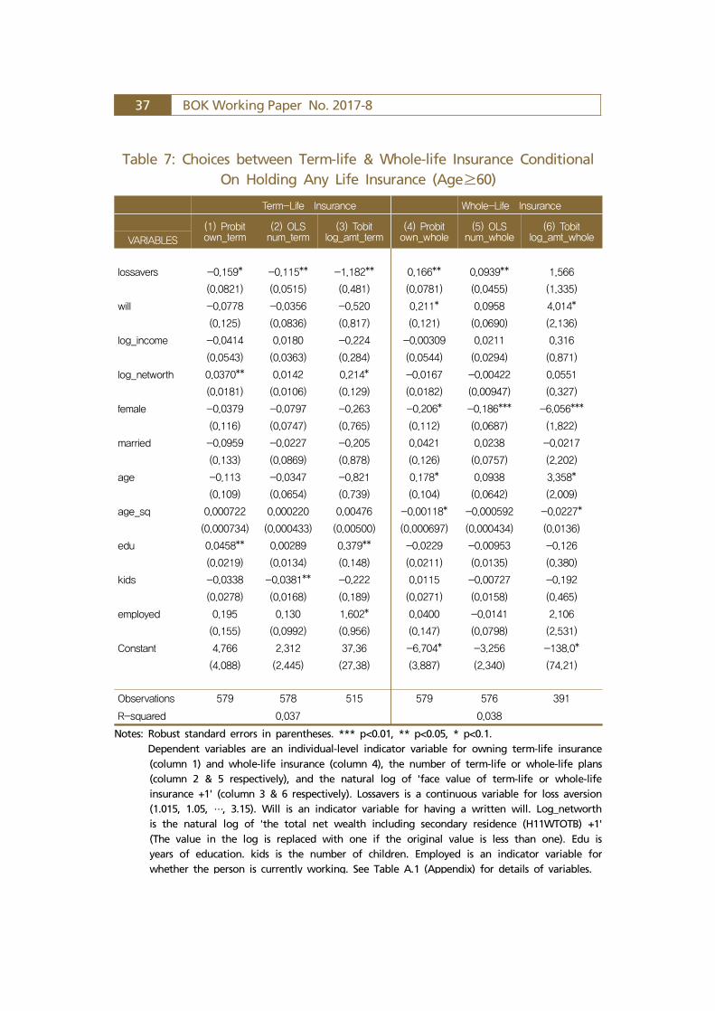
Table 7 reports the regression results when samples are restricted to those

who own any type of life insurance. It shows that not only term-life insurance,

but also whole-life insurance, has a statistically significant relationship with

loss-aversion. Columns (4)-(5) show that the positive association between

whole-life insurance ownership and loss-aversion becomes statistically

significant when we focus on the choices between term-life and whole-life

insurance. The marginal effects of loss-aversion measured at means of

explanatory variables of Table 7 are as follows: for those who own any type of

life insurance, a one-unit change in loss aversion marginally decreases

(increases) the probability of owning term-life (whole-life) insurance by 5.83

(6.60) percent point if the marginal effect is measured at means of explanatory

variables. And one-unit increase in loss aversion decreases (increases) the

number of term-life (whole-life) policies by 0.115 (0.094), and decreases

(increases) the desired coverage amount of term-life (whole-life) by 118.2

(156.6) percent point.

The effect of a bequest motive on term-life and whole-life insurance appears

to be in line with the prediction [A4] of the model: the desire for leaving

bequests for an expected death at a later time ( ) increases the demand for

saving. Table 6 and Table 7 report that the bequest motive as measured by an

indicator variable if an individual has a written will is positively associated with

whole-life insurance. Although the act of writing a will is open to interpretation,

when the problem is narrowed down as to whether the act is associated with

or , it is reasonable to interpret that the act is associated with .


An indicator variable for being currently employed is estimated to be

significantly positively associated with term-life insurance but not with

whole-life insurance. This result is consistent with the fact that (i) those with

labor income are more likely to purchase term-life insurance because one

primary function of term-life insurance is to replace labor income in the event

of an income earner’s death; and (ii) current workers are more likely to be

covered by the employer-provided term-life plan.


Table 6: Loss Aversion, Term-life & Whole-life Insurance (Age≥60)

Panel A. Simple Regression　　 Term-Life Insurance 　 Whole-Life Insurance

　 (1) Probitown_term

(2) OLSnum_term

(3) Tobitlog_amt_term

(4) Probitown_whole

(5) OLSnum_whole

(6) Tobitlog_amt_wholeVARIABLES

　　　　　　　

lossavers -0.0984* -0.0695* -1.685** 0.0974 0.0456* 0.919　 (0.0568) (0.0357) (0.664) (0.0606) (0.0273) (1.404)Constant -0.0814 0.674*** -0.380 -0.893*** 0.223*** -24.73***　 (0.161) (0.103) (1.930) (0.173) (0.0760) (4.156)　　　　　　　

Observations 1,051 1,050 987 1,051 1,048 862R-squared 　 0.004 　　 0.002 　　　　　　　　

Panel B. Regressions with control variables　　 Term-Life Insurance 　 Whole-Life Insurance　 (1) Probit

own_term(2) OLS

num_term(3) Tobit

log_amt_term(4) Probit

own_whole(5) OLS

num_whole(6) Tobit

log_amt_wholeVARIABLES　　　　　　　

lossavers -0.0964* -0.0674* -1.337** 0.0984 0.0452 0.834　 (0.0583) (0.0351) (0.629) (0.0619) (0.0276) (1.394)will 0.0456 0.0299 0.341 0.213** 0.0882** 5.597**　 (0.0950) (0.0578) (1.070) (0.0992) (0.0447) (2.288)log_income 0.0179 0.0235 0.113 0.0265 0.0193 0.574　 (0.0369) (0.0203) (0.416) (0.0334) (0.0131) (0.830)log_networth 0.0379*** 0.0152** 0.391** 0.00712 0.00425 0.301　 (0.0134) (0.00621) (0.159) (0.0131) (0.00484) (0.311)female -0.115 -0.0874* -0.976 -0.216** -0.142*** -7.232***　 (0.0852) (0.0507) (0.971) (0.0874) (0.0431) (1.860)married -0.0430 -0.00415 0.147 0.00991 0.00903 -0.0943　 (0.0966) (0.0570) (1.107) (0.100) (0.0474) (2.253)age -0.0568 -0.0243 -0.707 0.146* 0.0567 3.351　 (0.0764) (0.0412) (0.888) (0.0875) (0.0386) (2.169)age_sq 0.000300 0.000125 0.00323 -0.00101* -0.000380 -0.0234　 (0.000513) (0.000272) (0.00600) (0.000590) (0.000259) (0.0147)edu 0.0441*** 0.0122* 0.554*** 0.00750 0.00319 0.143　 (0.0144) (0.00705) (0.167) (0.0153) (0.00709) (0.369)kids 0.00284 -0.00962 0.0388 0.0246 0.00426 0.00502　 (0.0199) (0.0102) (0.227) (0.0205) (0.00929) (0.437)employed 0.218** 0.145** 2.698** 0.113 0.0277 3.602　 (0.108) (0.0666) (1.173) (0.115) (0.0514) (2.452)Constant 1.269 1.243 20.00 -6.649** -2.136 -153.6*　 (2.852) (1.547) (33.09) (3.240) (1.410) (78.68)　　　　　　　

Observations 1,042 1,041 978 1,042 1,039 854R-squared 　 0.047 　　 0.029 　

Notes: Robust standard errors in parentheses. *** p<0.01, ** p<0.05, * p<0.1. Dependent variables are individual-level indicator variables for owning term-life or whole-life

insurance (column 1 & 4 respectively), the number of term-life or whole-life plans (column 2 & 5 respectively), and the natural log of 'face value of term-life or whole-life insurance +1' (column 3 & 6 respectively). Lossavers is a continuous variable for loss aversion (1.015, 1.05, …, 3.15). Will is an indicator variable for having a written will. Log_networth is the natural log of 'the total net wealth including secondary residence (H11WTOTB) +1' (The value in the log is replaced with one if the original value is less than one). Edu is years of education. Kids is the number of children. Employed is an indicator variable for the person is currently working.


Table 7: Choices between Term-life & Whole-life Insurance Conditional On Holding Any Life Insurance (Age≥60)

　　 Term-Life Insurance 　 Whole-Life Insurance


(2) OLSnum_term


(4) Probitown_whole

(5) OLSnum_whole


　　　　　　　

lossavers -0.159* -0.115** -1.182** 0.166** 0.0939** 1.566

　 (0.0821) (0.0515) (0.481) (0.0781) (0.0455) (1.335)

will -0.0778 -0.0356 -0.520 0.211* 0.0958 4.014*

　 (0.125) (0.0836) (0.817) (0.121) (0.0690) (2.136)

log_income -0.0414 0.0180 -0.224 -0.00309 0.0211 0.316

　 (0.0543) (0.0363) (0.284) (0.0544) (0.0294) (0.871)

log_networth 0.0370** 0.0142 0.214* -0.0167 -0.00422 0.0551

　 (0.0181) (0.0106) (0.129) (0.0182) (0.00947) (0.327)

female -0.0379 -0.0797 -0.263 -0.206* -0.186*** -6.056***

　 (0.116) (0.0747) (0.765) (0.112) (0.0687) (1.822)

married -0.0959 -0.0227 -0.205 0.0421 0.0238 -0.0217

　 (0.133) (0.0869) (0.878) (0.126) (0.0757) (2.202)

age -0.113 -0.0347 -0.821 0.178* 0.0938 3.358*

　 (0.109) (0.0654) (0.739) (0.104) (0.0642) (2.009)

age_sq 0.000722 0.000220 0.00476 -0.00118* -0.000592 -0.0227*

　 (0.000734) (0.000433) (0.00500) (0.000697) (0.000434) (0.0136)

edu 0.0458** 0.00289 0.379** -0.0229 -0.00953 -0.126

　 (0.0219) (0.0134) (0.148) (0.0211) (0.0135) (0.380)

kids -0.0338 -0.0381** -0.222 0.0115 -0.00727 -0.192

　 (0.0278) (0.0168) (0.189) (0.0271) (0.0158) (0.465)

employed 0.195 0.130 1.602* 0.0400 -0.0141 2.106

　 (0.155) (0.0992) (0.956) (0.147) (0.0798) (2.531)

Constant 4.766 2.312 37.36 -6.704* -3.256 -138.0*

　 (4.088) (2.445) (27.38) (3.887) (2.340) (74.21)

　　　　　　　

Observations 579 578 515 579 576 391

R-squared 　 0.037 　　 0.038 　

Notes: Robust standard errors in parentheses. *** p<0.01, ** p<0.05, * p<0.1. Dependent variables are an individual-level indicator variable for owning term-life insurance

(column 1) and whole-life insurance (column 4), the number of term-life or whole-life plans (column 2 & 5 respectively), and the natural log of 'face value of term-life or whole-life insurance +1' (column 3 & 6 respectively). Lossavers is a continuous variable for loss aversion (1.015, 1.05, …, 3.15). Will is an indicator variable for having a written will. Log_networth is the natural log of 'the total net wealth including secondary residence (H11WTOTB) +1' (The value in the log is replaced with one if the original value is less than one). Edu is years of education. kids is the number of children. Employed is an indicator variable for whether the person is currently working. See Table A.1 (Appendix) for details of variables.


Interaction with the expected survival probability

This paper now addresses the prediction [A5]: if the effect of loss aversion

on insurance demand is amplified by the degree of narrow framing and the

expected survival probability. First, it examines if the negative effect of loss

aversion is more prominent among those who expect that they will not die in

the near future (those who expect that they are more likely to lose premiums if

they purchase term-limited insurance). To measure the expected survival

probability, the HRS question is used, which asks the percent chance that a

respondent will live at least 11~15 more years (prob_live80100). A dummy

variable, livesure, indicates that the respondent responds 90~100 percent to

the question. Column (3) of Table 8 reports a significant negative coefficient of

the interaction term (lossavers×livesure) in the regressions for own_term and

log_amt_term, indicating that the effect of loss aversion is indeed large among

those who expect that they will live 11~15 more years with the probability of 90

percent or more. Columns (2) of Table 8, however, show that the interaction

term is not significant in the regression for num_term. Another result to note is

that the expected survival probability itself (prob_live80100) shows a positive

sign, not a negative sign, as the model has predicted, although all coefficients

are not statistically significant. Overall, while some of the results are in line with

the model’s prediction, there are somewhat weaker results in terms of loss

aversion’s interaction with the expected survival probability.


Table 8: Interaction between Loss Aversion and the Expected Survival Probability (Age≥60)



(2) OLSnum_term


(4) Probitown_whole

(5) OLSnum_whole


　　　　　　　

lossavers -0.0843 -0.0621* -1.144* 0.108* 0.0467 0.893

　 (0.0605) (0.0370) (0.642) (0.0646) (0.0292) (1.415)

lossavers x livesure -0.0590* -0.0193 -0.912** -0.00700 0.00199 -0.609

　 (0.0359) (0.0184) (0.433) (0.0371) (0.0200) (0.839)

prob_live80100 0.00219 9.84e-05 0.0309 0.000772 0.000489 0.0422

　 (0.00171) (0.00103) (0.0191) (0.00177) (0.000829) (0.0380)

will 0.0474 0.0393 -0.0719 0.185* 0.0796* 5.531**

　 (0.0981) (0.0598) (1.091) (0.102) (0.0470) (2.303)

log_income -0.00395 0.0166 -0.0957 0.0328 0.0214 0.389

　 (0.0381) (0.0221) (0.415) (0.0358) (0.0144) (0.795)

log_networth 0.0387*** 0.0154** 0.384** 0.00847 0.00500 0.324

　 (0.0138) (0.00658) (0.161) (0.0136) (0.00510) (0.314)

female -0.107 -0.0859 -0.849 -0.230** -0.148*** -7.485***

　 (0.0888) (0.0534) (1.005) (0.0904) (0.0451) (1.867)

married -0.0246 -0.0100 0.308 0.0108 0.00613 -0.296

　 (0.100) (0.0594) (1.134) (0.104) (0.0499) (2.266)

age -0.0765 -0.0383 -1.386 0.264** 0.0826 3.719

　 (0.109) (0.0620) (1.238) (0.116) (0.0572) (2.712)

age_sq 0.000446 0.000224 0.00816 -0.00183** -0.000559 -0.0261

　 (0.000750) (0.000423) (0.00858) (0.000801) (0.000395) (0.0187)

edu 0.0431*** 0.0126* 0.537*** 0.00444 0.00153 0.0915

　 (0.0150) (0.00753) (0.170) (0.0161) (0.00768) (0.376)

kids 0.00908 -0.00569 0.0646 0.0185 0.000528 -0.0685

　 (0.0207) (0.0108) (0.231) (0.0212) (0.00978) (0.446)

employed 0.252** 0.166** 2.940** 0.103 0.0214 3.517

　 (0.111) (0.0691) (1.192) (0.117) (0.0535) (2.449)

Constant 2.015 1.766 44.12 -10.88*** -3.074 -164.5*

　 (3.940) (2.244) (44.59) (4.213) (2.029) (96.90)

　　　　　　　

Observations 968 967 911 968 965 791

R-squared 　 0.046 　　 0.030 　

Notes: Robust standard errors in parentheses. *** p<0.01, ** p<0.05, * p<0.1. prob_live80100 is the respondents' subjective expectation on the percent chance that he/she will live at least 11~15 more years. It is based on the question "What is the percent chance that you will live to be [85/80/90/95/100] or more? (00-10-20-…-100). [Assigned ages are as follows: 80 (IF AGE IS 65-69) 85 (IF AGE IS 70-74) 90 (IF AGE IS 75-79) 95 (IF AGE IS 80-84) 100 (IF AGE IS 85-89)]. Livesure is an indicator variable for prob_live80100 being 90-100 percent. See Table A1 (Appendix) for details of variables.


Interaction with the degree of narrow framing (proxied by the inverse of taking financial advice)

Kahneman (2003) points out that narrow framing is associated with the “low

accessibility” to a person’s existing risk and portfolio. This paper posits that

those who have taken financial advice from financial experts are more likely to

have realized his/her existing risk and thus are more likely to have broad framing rather than narrow framing. Financial advice may also have direct

impact on life insurance take-up because financial experts may encourage

individuals to purchase a life insurance plan. To capture these effects, the HRS

2014 module question regarding financial advice is used. The variable, advice,

is an indicator variable for whether a person takes financial advice from experts

(e.g., bank officer, financial consultant). When the ‘advice’ variable is merged

with the loss aversion data, there are fewer than one hundred samples.

Although the sample size is less than ideal, interesting patterns that are

consistent with the model are found in the regression results. First, the sign of

the interaction term (i_lossaver×advice) is positive in columns (1)-(3) and

negative in columns (4)-(6), which is consistent with the prediction of the

model. The results imply that the effect of loss aversion on insurance uptake is

canceled out by financial advice. However, only three interaction terms are

statistically significant. Direct effects of financial advice on term-life and

whole-life ownership (apart from the interaction effect with loss aversion) are

captured by the ‘advice’ term, but all of them are insignificant.


Table 9: Interaction between Loss Aversion and Narrow Framing (Proxied by the Inverse of Taking Financial Advice, Age≥60)

　　 Term-Life Insurance 　 Whole-Life Insurance　 (1) Probit

own_term(2) OLS

num_term(3) Tobit


own_whole(5) OLS

num_whole(6) Tobit

log_amt_wholeVARIABLES　　　　　　　lossavers -0.455* -0.214* -4.504** 0.523** 0.190** 71.74***

　 (0.233) (0.108) (1.953) (0.237) (0.0756) (0.732)i_lossaver_advice 0.915 0.555* 10.38 -2.294** -0.627* -161.0

　 (0.914) (0.324) (8.228) (1.065) (0.360) (0)

advice -0.536 -0.374 -4.574 1.314 0.395 81.36

　 (0.759) (0.240) (6.620) (0.846) (0.246) (0)will -0.709* -0.251 -5.375 0.764* 0.250 21.96***

　 (0.416) (0.160) (4.016) (0.396) (0.156) (2.001)

log_income 0.281 0.143 3.829 0.0583 0.0582 6.659***

　 (0.257) (0.116) (2.452) (0.248) (0.119) (0.216)log_networth 0.0189 0.00472 0.161 0.0847* 0.0174 0.0112

　 (0.0473) (0.0170) (0.475) (0.0446) (0.0144) (0.182)

female 0.221 0.0452 1.774 -0.442 -0.165 -2.281

　 (0.333) (0.119) (3.446) (0.344) (0.161) (1.756)married -0.443 -0.171 -4.746 -0.200 -0.0352 2.996

　 (0.422) (0.159) (4.329) (0.435) (0.191) (1.968)

age -0.0245 -0.00482 -0.392 -0.00556 -0.00341 -0.897***

　 (0.0256) (0.00867) (0.282) (0.0213) (0.00905) (0.0322)

edu 0.0618 0.0193 0.188 -0.0721 -0.0232 -2.020***　 (0.0647) (0.0199) (0.570) (0.0552) (0.0290) (0.165)

kids 0.0580 0.0166 0.859 0.154* 0.0542 2.665***

　 (0.0794) (0.0326) (0.778) (0.0858) (0.0391) (0.366)

employed 0.151 0.162 0.658 0.295 -0.0150 -6.983***　 (0.437) (0.200) (4.366) (0.465) (0.183) (1.422)

Constant -1.165 -0.372 -7.535 -3.072 -0.649 -241.8***

　 (3.423) (1.319) (36.30) (3.003) (1.507) (2.307)　　　　　　　Observations 92 92 90 91 91 73R-squared 　 0.246 　　 0.110 　

Notes: Robust standard errors in parentheses. *** p<0.01, ** p<0.05, * p<0.1. Advice is an indicator variable for getting advice from financial experts. It is based on the

2014 HRS Module questions "Do you [and your[partner/husband/wife]] have someone such as a friend or relative, or bank officer, lawyer or financial consultant who regularly helps you with handling your money or property or other financial matters such as signing checks, paying bills, dealing with banks and making investments? [Yes /No]" and "[IF YES] Who helps you [and your [partner/husband/wife]] with your finances? 1. Child Or Child-In-Law, 2. Other Relative, 3. Friend, 4. Lawyer, 5. Bank Officer, 6. Financial Consultant, Accountant Or Other Professional Investment Counselor, 7. Other, Specify." The value of zero is assigned if a respondent chooses "No" to the first question or "1~4, or 7" to the second question. The value of one is assigned if a respondent choose Yes in the first question and (5 or 6) in the second question (getting help from financial experts).


Robustness checks

First, the possible effect of employer-provided term-life insurance is further

controlled for. The dependent variable of columns (1)-(2) in Panel A of Table

A.7 (Appendix) is an indicator variable for owning two or more policies of

term-life insurance. The dependent variable of columns (3)-(4) is the log of the

“coverage amount of term-life insurance $50,000” (the dependent variable is

replaced with 0 if the coverage amount is less than $50,001). By using these

dependent variables, we consider the possibility that one term-life insurance

plan with the coverage amount of $50,000 or less can be provided by

employers. The results in columns (1)-(3) of Panel A show that the negative

effect of loss aversion on term-life insurance is significant even if the possibility

that the first term-life insurance policy is provided by employers is considered.

In the case of column (4), loss aversion is only marginally significant (p-value:

13.2 percent). However, in this case also, loss aversion maintains its negative

sign. In Panel B of Table A.7 (Appendix), regression results are reported when

13 occupation dummy variables based on industry codes with the longest

reported tenure are added. There are still significant coefficients of loss

aversion in the regressions for term-life insurance.

Second, the sample is restricted to low-wealth individuals to consider the

possibility that (i) the level of wealth may affect individuals’ attitude toward loss

and (ii) to control for the heterogeneous tax-exemption or tax-deference effects

of life insurance that differs by wealth levels (Brown 2001). In particular, the

possibility that wealth levels co-determine loss aversion (in the form of

decreasing absolute risk aversion (DARA) or increasing absolute risk aversion

(IARA)) and life insurance ownership decisions can be ruled out by looking at

similar wealth-level individuals. This study chooses low-wealth individuals who

are less likely to be affected by tax incentives of whole-life insurance. The results

in Table A.8 (Appendix) show that statistical significance is somewhat weakened

from the baseline results as the sample size has halved. Still, loss aversion is

significant at 5 percent in the regression for num_term and at 10 percent in the

regression for log_amt_term.

Third, a risk-aversion measure is added to address a possible omitted


variable problem. The status-quo-bias-free lifetime income gamble questions by

Barsky et al. (1997) are used to measure risk-aversion. Note that the lifetime

income gamble questions capture the concavity of Bernoulli’s utility-of-wealth

function, which represents risk attitude when the magnitude of risk is large and

when all risks are assessed comprehensively within a broad frame. This

contrasts with the loss-aversion questions capturing the concavity of Kahneman

and Tversky’s (1979, 1992) value function when the magnitude of risk is small

and when each risk is likely to be assessed in isolation from each other. (See

Table 1 and Figure 3). The number of observations in which both risk-aversion

and loss-aversion measures are available is about 360. Panel A in Table A.9

(Appendix) reports that loss aversion maintains its significant negative sign in

the regressions for term-life insurance holdings and shows a positive sign in the

regressions for whole-life holdings. One thing to note is that the risk-aversion

measure shows a significant negative sign in the regression for whole-life

insurance. To further examine the relationship between risk aversion and life

insurance holdings, the loss-aversion measure is dropped from explanatory

variables so that the relationship can be tested in a large sample. When loss

aversion is dropped from the covariates, available observations increase to about

4,000 individuals. In this large data set, risk aversion is found to be an

insignificant variable in the regressions for whole-life insurance (See Panel B of

Table A.9 (Appendix)). This relationship between risk aversion and life

insurance holdings is further explained using an age cohort sample.

Fourth, the sample is restricted to those in the same life-cycle stage, those

aged 60-69 in particular. Table A.10 (Appendix) reports the results. These

results are similar to the previous results: loss aversion is significantly negatively

associated with term-life insurance and is positively associated with whole-life

insurance. Note that even if the risk aversion measure is added to this age

cohort sample, loss aversion’s effects remain robust while risk-aversion is not

significant (Panel B of Table A.10, Appendix). Another pattern to note is that,

although statistically insignificant, risk aversion tends to be positively associated

with term-life insurance ownership and negatively associated whole-life

insurance ownership. This pattern is consistent with the rational aspects of


purchasing insurance.

Fifth, the Bivariate Probit, SUR, and Bivariate Tobit models are employed to

consider the cases where decisions to buy term-life and whole-life are jointly

determined.14) Since term-life and whole-life insurance are partial substitutes of

each other, owning one type of life insurance may have a negative effect on the

purchase of the other type of life insurance. Results for Bivariate Probit model

for two binary outcomes (own_term, own_whole) are reported in columns (1)-(2)

in Table A.11 (Appendix). Although the estimated coefficients of loss-aversion

are similar to the baseline results in Table 6 (two separate Probit models), the

correlation () between term-life and whole-life ownership is estimated to be

–0.232 and significant at 1%. This indicates that the two types of life insurance

are indeed partial substitutes of each other. This negative correlation is in line

with previous literature, such as Frees and Sun (2010). Columns (3)-(4) report

SUR estimation results for the number of plans, which can be more efficient

than two separate OLS regressions. Columns (5)-(6) report estimation results of

the Bivariate Tobit model for the coverage amount. The results are not

significantly different from those in Table 6.

Sixth, an indicator variable is used for high loss-aversion rather than using a

continuous measure for loss aversion. The indicator variable (i_lossaver) takes

the value of one if a person’s loss aversion is greater than three and zero

otherwise. Table A.12 (Appendix) reports similar results to those in Table 6.

Lastly, another control variable, self-reported health status is added to

control for the possible adverse selection problem in the life insurance market.

One can verify that the results in Table A.13 (Appendix) are similar to the

baseline results.

4.3.3 Regression Results 2: Loss Aversion and Household Wealth

This section examines if loss aversion increases savings (Prediction [A2]) by

looking at loss-aversion’s association with households’ wealth levels. Since the

logged wealth variables are left-censored at zero, the Tobit model is employed.

14) For estimation, Stata codes ‘biprobit’, ‘sureg’, and ‘mvtobit’ are used.


Analyzed samples are restricted to those aged 65 or more so that the focus is on

those who have entered the retirement stage and hence finished their wealth

accumulation processes. Columns (1) and (6) in Table 10 report that loss

aversion is negatively associated with log_Stock, which represents the sum of the

amount of stocks, mutual funds, and investment trusts a household holds. This

negative association is consistent with the model (loss-averse individuals are less

likely to hold risky-looking assets) and the literature on loss-aversion and stock

market participation (Dimmock & Kouwenberg, 2010). Columns (3) and (8)

report that loss aversion is positively associated with log_Nonrisky, the amount

of non-risky assets as measured by the sum of the ‘value of checking, savings, or

money market accounts,’ ‘value of CD, government savings bonds, and T-bills,’

and the ‘net value of bonds and bond funds.’ Columns (5) and (10) show that

loss aversion is positively associated with Net Worth, the sum of household’s net

financial asset and real estate asset, including secondary residences. These

results are in line with the prediction [A2].

Another result to note is that having a written will is significantly positively

associated with levels of wealth. (columns (6)-(10) in Table 10). Although our

estimation strategy does not resolve the possible reverse causality issue (i.e.,

wealthy individuals are more likely to write a will), the strong positive

correlation is in line with the model’s prediction [A4].


Table 10: Loss Aversion and Household Wealth (Tobit Model, Age≥65)

　 (1)log_Stock

(2)log_House

(3) log_Nonrisky

(4) log_NetFinWorth

(5) log_NetWorth

(6)log_Stock

(7) log_House

(8) log_Nonrisky

(9) log_NetFinWorth

(10) log_NetWorthVARIABLES

　　　　　　　　　　　

lossavers -1.560* 0.378 0.571** 0.501 0.489** -1.964** 0.300 0.443* 0.256 0.333**

　 (0.871) (0.321) (0.250) (0.315) (0.228) (0.839) (0.295) (0.228) (0.291) (0.166)

log_income 5.978*** 0.859*** 1.154*** 1.695*** 0.776*** 3.764*** 0.310 0.802*** 1.033*** 0.230**

　 (0.734) (0.288) (0.275) (0.396) (0.206) (0.818) (0.214) (0.232) (0.306) (0.106)

edu 1.621*** 0.296*** 0.535*** 0.669*** 0.315*** 1.100*** 0.156* 0.283*** 0.375*** 0.159***

　 (0.252) (0.0819) (0.0658) (0.0880) (0.0532) (0.265) (0.0845) (0.0662) (0.0861) (0.0410)

age 0.161* -0.0917*** 0.0661*** 0.128*** -0.00856 3.036 0.562 -0.315 0.510 0.0634

　 (0.0916) (0.0336) (0.0238) (0.0307) (0.0190) (1.850) (0.605) (0.445) (0.541) (0.272)

age_sq 　　　　　 -0.0194 -0.00410 0.00232 -0.00265 -0.000321

　　　　　　 (0.0120) (0.00393) (0.00286) (0.00346) (0.00173)

will 　　　　　 10.05*** 2.273*** 2.351*** 3.603*** 1.859***

　　　　　　 (1.579) (0.476) (0.360) (0.481) (0.245)

female 　　　　　 2.801** 0.437 0.442 0.630 0.186

　　　　　　 (1.294) (0.436) (0.333) (0.442) (0.219)

married 　　　　　 4.569*** 3.167*** 0.817** 1.417*** 0.979***

　　　　　　 (1.497) (0.486) (0.360) (0.488) (0.227)

kids 　　　　　 -0.984*** 0.0382 -0.0909 -0.117 0.00492

　　　　　　 (0.331) (0.0923) (0.0723) (0.0951) (0.0488)

employed 　　　　　 -2.153 -0.0501 -0.428 -0.440 0.476

　　　　　　 (2.002) (0.616) (0.471) (0.657) (0.314)

i_hispanic 　　　　　 -16.57*** -0.754 -2.639*** -2.749*** -0.453

　　　　　　 (5.175) (0.935) (0.811) (0.979) (0.495)

own_house 　　　　　 1.873 　 1.305*** 1.843*** 4.539***

　　　　　　 (1.945) 　 (0.445) (0.563) (0.387)

Constant -99.45*** 1.749 -17.75*** -29.93*** -1.512 -182.2** -20.69 1.535 -36.97* -2.746

　 (11.02) (4.201) (3.649) (5.030) (2.855) (71.35) (23.22) (17.23) (21.05) (10.56)

occupation_dummies

- - - - - O 　 O O O

Observations 834 834 834 834 834 829 829 829 829 829

Notes: Robust standard errors in parentheses. *** p<0.01, ** p<0.05, * p<0.1. Occupation_dummies are 13 dummy variables based on the industry code for job with

longest tenure (RAND HRS code: R11JLIND). Own_house is an indicator variable for owning house (H11WOHOUS).

Robustness checks

First, we apply quantile regressions because asset holdings data can be

sensitive to extreme values. Results in Table 11 report median regression results

in columns (2)-(5) and a 95 percentile regression result in column (1).15) Similar

15) A 95 percentile quantile regression is applied because only about 11 percent of households participate in the stock market.


to the results in Table 10, loss aversion has a positive association with

log_NetWorth and log_Nonrisky and a negative association with log_Stock.

Figure 5 shows the coefficients of loss-aversion when quantile regressions with

various percentiles are applied. It shows that loss aversion’s effects on asset

holdings differ depending on wealth quantiles. Loss aversion’s effects are

significant among low-to-moderate wealth households.

Second, the sample is restricted to those in the same life-cycle stage, those

aged 65-70 in particular. The results in Table A.14 show that, although

statistical significance has been weakened, loss-aversion’s association with

log_Stock and log_NetWorth remains similar to the baseline results in Table 10.

Third, the indicator variables are used for high loss aversion (i_lossaver,

i_lossaver2) rather than using a continuous variable for loss aversion. The

results in Table A.15 (Appendix) show that, although statistical significance

varies depending on the types of dummy variables, the overall results are

similar to the baseline results in Table 10.

Fourth, the risk-aversion measure (Barsky et al., 1997) is added to address a

possible omitted variable problem. The number of observations in which both

risk-aversion and loss-aversion measures are available is only 197. Table A.16

(Appendix) reports that loss aversion has a significant negative sign in the

regression for log_stock (Column 1). Loss aversion maintains its positive sign in

the regression for log_NetWorth but the coefficient is not statistically significant

(Column 5). Another point to note is that, in all columns (1)-(5), the risk

aversion measure is not statistically significant. To further check if the

insignificance of the risk aversion measure is caused by too few samples, the

loss-aversion measure is dropped from explanatory variables so that the

relationship between risk aversion and wealth can be tested in a large sample.

When loss aversion is dropped from covariates, available observations increase

to 2,215 individuals. In this large data set, risk aversion is found to be an

insignificant variable in all regressions (Columns 6-10 in Table A.16). These

results suggest that the risk aversion measure does not have an additional

explanatory power on wealth levels when demographic variables are controlled

for. This, in turn, implies that although the main regression results do not


include the risk aversion measure, the results may not have an omitted variable

problem caused by the exclusion of the risk aversion measure.16)

Lastly, share by asset type (or asset-specific share) of net worth is used as a

dependent variable. Table A.17 reports the Tobit regression results. It shows

that, consistent with the prediction of this paper, the Stock’s share is

significantly negatively associated with loss aversion while Nonrisky’s share is

positively associated with loss aversion. But in the case of Nonrisky’s share,

statistical significance is lacking.

16) Note that most empirical studies on insurance purchasing behavior have used demographic variables (e.g., age, gender, family structure) as a proxy for risk aversion instead of using direct measures for risk aversion due to the difficulty of obtaining an appropriate risk aversion measure (Outreville, 2014, p. 170). Recent studies by Hwang (2016a) and Gottlieb and Mitchell (2015) report that the CRRA measure is not a statistically significant determinant of take-up of long-term care insurance or private health insurance.

Table 11: Loss Aversion and Household Wealth (Quantile Regression, Age≥65)

　 (1)

log_Stock

(2)

log_House

(3)

log_Nonrisky

(4)

log_NetFinWorth

(5)

log_NetWorthVARIABLES

quantile 0.95 0.5 0.5 0.5 0.5　　　　　　

lossavers -0.506** 0.163* 0.373* 0.0171 0.218**

　 (0.236) (0.0985) (0.199) (0.260) (0.0929)

log_income 1.110*** 0.426*** 1.166*** 1.328*** 0.838***

　 (0.137) (0.0570) (0.115) (0.151) (0.0538)

age 0.0367 -0.0100 0.0699*** 0.0866*** -0.00423

　 (0.0230) (0.00958) (0.0194) (0.0253) (0.00904)

edu 0.466*** 0.110*** 0.422*** 0.555*** 0.178***

　 (0.0549) (0.0229) (0.0462) (0.0605) (0.0216)

Constant -6.635*** 5.824*** -15.05*** -18.31*** 0.953

　 (2.440) (1.017) (2.055) (2.689) (0.960)　　　　　　

Observations 834 834 834 834 834

Notes: Standard errors in parentheses. *** p<0.01, ** p<0.05, * p<0.1.


Figure 5: Coefficients of Loss Aversion by Quantiles when Quantile Regressions are Estimated at All Percentiles (Specification: Columns

(2)-(5) of Table 11)

Log_House

Log_Nonrisky

Log_NetFinWorth Log_NetWorth

Notes: Shaded regions indicate the 95% confidence interval of quantile regressions when dependent variables are log_House, log_Nonrisky, log_NetFinWorth, and log_NetWorth (columns (2)-(5) of Table 11). Bold lines in the center of the shaded regions indicate the effects of loss aversion on log_House (by qunatiles of log_House), log_Nonrisky (by quantiles of log_Nonrisky), log_NetFinWorth (by quantiles of log_NetFinWorth), and on log_NetWorth (by quantiles of log_NetWorth). Straight dotted lines indicate the coefficient and 95% confidence intervals of OLS regressions.


Ⅴ. Summary

The modeling part of this paper examines how loss aversion would affect

insurance buying decisions and savings decisions within the context of life

cycle/permanent income savings model with a bequest motive. The five testable

predictions from the model are first derived and then tested empirically. Loss

aversion is measured by respondents’ attitudes toward small-amount risky

investments (e.g., equal chances of receiving $115 or paying $100;...; receiving

$300 or paying $100) in the HRS 2012. This paper focuses on the three types

of assets that differ from each other in the insurance vs. savings element: (1)

term-life insurance (pure insurance), (2) whole-life insurance (partial insurance

+ partial savings), and (3) net worth (savings).

First three predictions ([A1]-[A3]) can be summarized as follows: while loss

aversion decreases the demand for pure insurance (term-life insurance), it may

increase the demand for savings (net worth). Loss-aversion may have either a

negative or a positive impact on the holdings of whole-life insurance, since

whole-life insurance is a combination of pure insurance and savings. The sign

of the impact will be determined by the proportion of protection vs. savings

elements that a whole-life insurance plan contains. Empirical test results using

the HRS data set are consistent with these predictions. Loss-averse elderly

people have a significantly low ownership ratio of term-life insurance. They also

have a lower number of term-life policies and lower coverage amounts of

term-life insurance. In contrast, loss-averse elderly people possess higher levels

of net worth than others in the form of non-risky assets. In its relationship with

whole-life insurance, loss-aversion shows a positive association with whole-life

insurance holdings, but its statistical significance is less robust. This occasional

positive association is consistent with the fact that whole-life insurance held by

the elderly has considerable savings elements.

The model’s fourth prediction ([A4]) is that two weights for bequests

(bequest weight for the death at t+1 vs. bequest weight for the death at t+2)

have different impacts on term-life insurance and savings. In particular, the

model predicts that an increase in the bequest weight for t+2 (expected death)


would decrease the demand for term-life insurance, while it would increase the

demand for savings. Empirical results are in line with this prediction. The

bequest motive for expected death as measured by an indicator variable for

having a written will is not significant in the regressions for term-life insurance

holdings but significant with a positive sign in the regressions for whole-life

insurance holdings. The indicator variable for the bequest motive shows the

strongest association with levels of net worth, which represents pure savings.

The model’s fifth prediction ([A5]) is that the effect of loss-aversion on the

demand for term-life insurance is amplified by the expected survival probability

and the degree of narrow framing. The findings are somewhat weaker but still

consistent with this prediction. For example, the negative effect of loss aversion

on the coverage amount of term-life is large among those who are confident

that they would not die in the near future.

The results in this paper suggest that loss aversion, one of the most common

behavioral tendencies, distorts the elderly’s portfolio choice substantially,

forcing the elderly to hold too little insurance and to save too much.17) This

implies that market failure or under-insurance problem may persist without

government’s intervention because the under-insurance problem is associated

with the deep-rooted loss aversion parameter (Guiso, 2015). This in turn

indicates that the provision of public insurance program may be needed to enhance

public welfare. Another implication of this paper is that under-insurance may

result in under-consumption through the channel of over-saving. As baby

boomers enter their retirement years, the elderly’s consumption will account for

more and more proportion of total consumption. The results in this paper

indicate that the provision of public insurance may be an effective measure to

stimulate the elderly’s consumption, thereby maintaining economic vitality in

the aging society.

The limitations of this paper are as follows. First, the empirical results in this

paper have a generalizability issue: this paper has not explored whether the

same results hold for the young because the samples of the HRS are limited to

17) Hwang (2016b) discusses the socially optimal level of insurance when individuals are subject to loss aversion and narrow framing.


those aged 51 and older by construction. Secondly, this paper uses several

proxy measures to test the predictions of the insurance-savings model, but the

proxy variables may be subject to measurement errors. For example, this paper

measures the strength of the bequest motives for expected death using an

indicator variable if an individual has a written will. The degree of narrow

framing is proxied by the inverse of taking financial advice. It should be

acknowledged that these proxy variables may be subject to measurement errors.

Thirdly, the current version of this paper limits the analysis to a cross-sectional

analysis. A dynamic analysis or panel study will help enrich and broaden our

understandings of the topic.

※ STATA replication codes (including the instructions for downloading the HRS public data) are available at https://drive.google.com/open?id=0B2f2_rE_k6lWRkxDSnFzMEVWdTA


References

Aizenman, J. (1998), “Buffer Stocks and Precautionary Savings with Loss Aversion,” Journal of international Money and Finance, Vol. 17(6), pp. 931-947.

Barberis, N. (2013), “Thirty Years of Prospect Theory in Economics: A Review and Assessment,” Journal of Economic Perspectives, Vol. 27(1), pp. 173-196.

Barberis, N., M. Huang, and T. Santos (2001), “Prospect Theory And Asset Prices,” Quarterly Journal of Economics, Vol. 116(1), pp. 1-53.

Barberis, N., M. Huang, and R. H. Thaler (2006), “Individual Preferences, Monetary Gambles, and Stock Market Participation: A Case for Narrow Framing,” The American Economic Review, Vol. 96(4), pp. 1069-1090.

Barsky, R. B., F. T. Juster, M. S. Kimball, and M. D. Shapiro (1997), “Preference Parameters And Behavioral Heterogeneity: An Experimental Approach In The Health And Retirement Study,” The Quarterly Journal of Economics.

Benartzi, S., and R. H. Thaler (1995), “Myopic Loss-aversion and the Equity Premium Puzzle,” Quarterly Journal of Economics, Vol. 110, pp. 73-92.

Benartzi, S., and R. H. Thaler (2007), “Heuristics and Biases in Retirement Savings Behavior,” The Journal of Economic Perspectives, Vol. 21(3), pp. 81-104.

Benartzi, S., A. Previtero, and R. H. Thaler (2011), “Annuitization Puzzles,” The Journal of Economic Perspectives, Vol. 25(4), pp. 143-164.

Bernheim, B. D., K. G. Carman, J. Gokhale, and L. J. Kotlikoff (2003), “Are Life Insurance Holdings Related to Financial Vulnerabilities?” Economic Inquiry, Vol. 41(4), pp. 531-554.

Bernheim, B. D., L. Forni, J. Gokhale, and L. J. Kotlikoff (2003), “The Mismatch between Life Insurance Holdings and Financial Vulnerabilities: Evidence from the Health and Retirement Study,” The American Economic Review, Vol. 93(1), pp. 354-365.


Brown, J. R. (2001), “Are the Elderly Really Over-annuitized? New Evidence on Life Insurance and Bequests,” In Themes in the Economics of Aging, University of Chicago Press, pp. 91-126.

Bhargava, S., G. Loewenstein, and J. Sydnor (2015), “Do Individuals Make Sensible Health Insurance Decisions? Evidence from a Menu with Dominated Options,” National Bureau of Economic Research, No. w21160.

Bowman, D., D. Minehart, and M. Rabin (1999), “Loss Aversion in a Consumption–savings Model,” Journal of Economic Behavior & Organization, Vol. 38(2), pp. 155-178.

Brown, J. R. (2014), “Income as the Outcome: How to Broaden the Narrow Framing of U.S. Retirement Policy,” Risk Management and Insurance Review, Vol. 17(1), pp. 7-16.

Brown, J. R., J. R. Kling, S. Mullainathan, and M. V. Wrobel (2008), “Why Don’t People Insure Late-Life Consumption? A Framing Explanation of the Under-annuitization Puzzle,” American Economic Review, Vol. 98(2), pp. 304-309.

Brown, J. R., J. R. Kling, S. Mullainathan, and M. V. Wrobel (2013), “Framing Lifetime Income,” The Journal of Retirement, Vol. 1(1), pp. 27-37.

Camerer, C. F. (2004), “Prospect Theory in the Wild: Evidence from the Field,” Advances in Behavioral Economics, pp. 148-161.

Cole, S., X. Giné, J. Tobacman, R. Townsend, P. Topalova, and J. Vickery (2013), “Barriers to Household Risk Management: Evidence from India,” American economic journal. Applied economics, Vol. 5(1), p. 104.

Chetty, R. (2015), “Behavioral Economics and Public Policy: A Pragmatic Perspective,” No. w20928, National Bureau of Economic Research.

Dimmock, S. G., and R. Kouwenberg (2010), “Loss-aversion and Household Portfolio Choice,” Journal of Empirical Finance, Vol. 17(3), pp. 441-459.


Dynan, K. E., J. Skinner, and S. P. Zeldes (2002), “The Importance of Bequests and Life-cycle Saving in Capital Accumulation: A New Answer,” The American Economic Review, Vol. 92(2), pp. 274-278.

Dynan, K. E., J. Skinner, and S. P. Zeldes (2004), “Do the Rich Save More?” Journal of political economy, Vol. 112(2), pp. 397-444.

Fischer, S. (1973), “A Life Cycle Model of Life Insurance Purchases,” International Economic Review, Vol. 14(1), pp. 132-152.

Frees, E. W., and Y. Sun (2010), “Household Life Insurance Demand: A Multivariate Two-part Model,” North American Actuarial Journal, Vol. 14(3), pp. 338-354.

Gottlieb, D. (2012), “Prospect Theory, Life Insurance, and Annuities,” The Wharton School Research Paper, No. 44.

Gottlieb, D., and O. S. Mitchell (2015), “Narrow Framing And Long-Term Care Insurance,” Pension Research Council Working Papers, 2015-03, Wharton School Pension Research Council, University of Pennsylvania.

Greene, M. R. (1963), “Attitudes toward Risk and a Theory of Insurance Consumption,” The Journal of Insurance, Vol. 30(2), pp. 165-182.

Greene, M. R. (1964), “Insurance Mindedness Implications for Insurance Theory,” The Journal of Risk and Insurance, Vol. 31(1), pp. 27-38.

Guiso, L. (2015), “A Test of Narrow Framing and its Origin,” Italian Economic Journal, Vol. 1(1), pp. 61-100.

Hwang, I. (2016a), “Prospect Theory and Insurance Demand. (February 3, 2016),” Available at SSRN: http://ssrn.com/abstract=2586360 or http://dx.doi.org/10.2139/ssrn.2586360.

Hwang, I. (2016b), “Behavioral Welfare Analysis of Insurance Markets: The Case of Narrow Framing and Loss Aversion (July 20, 2016),” Available at SSRN: https://ssrn.com/abstract=2673273.

Johnson, E. J., J. Hershey, J. Meszaros, and H. Kunreuther (1993), “Framing, Probability Distortions, and Insurance Decisions,” Journal of Risk and Uncertainty, Vol. 7(1), pp. 35-51.

http://ssrn.com/abstract=2586360


Kahneman, D. (2003), “Maps of Bounded Rationality: Psychology for Behavioral Economics,” American Economic Review, Vol. 93(5), pp. 1449-1475.

Kahneman, D., and D. Lovallo (1993), “Timid Choices and Bold Forecasts: A Cognitive Perspective on Risk Taking,” Management science, Vol. 39(1), pp. 17-31.

Kahneman, D., and A. Tversky (1979), “Prospect Theory: An Analysis of Decision under Risk,” Econometrica: Journal of the Econometric Society, Vol. 47(2), pp. 263-292.

Kőszegi, B., and M. Rabin (2009), “Reference-dependent Consumption Plans,” The American Economic Review, Vol. 99(3), pp. 909-936.

Kotlikoff, L. J. (1988), “Intergenerational Transfers and Savings,” Journal of Economic Perspectives, Vol. 2(2), pp. 41-58.

Kunreuther, H. C., M. V. Pauly, and S. McMorrow (2013), “Insurance and Behavioral Economics: Improving Decisions in the Most Misunderstood Industry,” Cambridge University Press.

Levin, I. P., S. L. Schneider, and G. J. Gaeth (1998), “All Frames are Not Ceated Equal: A Typology and Critical Analysis of Framing Effects,” Organizational Behavior and Human Decision Processes, Vol. 76(2), pp. 149-188.

LIMRA (2010), U.S. Life Ownership Study.

Mossin, J. (1968), “Aspects of Rational Insurance Purchasing,” The Journal of Political Economy, Vol. 76(4), pp. 553-568.

Mountain, T. (2015), “Life Insurance and Financial Vulnerability,” Doctoral Dissertation, The Ohio State University.

Outreville, J. F. (2014), “Risk Aversion, Risk Behavior, and Demand for Insurance: A Survey,” Journal of Insurance Issues, Vol. 37(2), pp. 158-186.

Pagel, M. (2016), “Expectations-based Reference-dependent Life-Cycle Consumption,” Available at https://sites.google.com/site/michaelapagel/.


Rabin, M. (2000), “Risk Aversion and Expected Utility Theory: A Calibration Theorem” Econometrica, Vol. 68(5), pp. 1281-1292.

Rabin, M., and R. H. Thaler (2001), “Anomalies: Risk Aversion,” The Journal of Economic Perspectives, Vol. 15(1), pp. 219-232.

Safra, Z., and U. Segal (2008), “Calibration Results for Non‐expected Utility Theories,” Econometrica, Vol. 76(5), pp. 1143-1166.

Simon, H. A. (1957), “Models of Man: Social and Rational,” John Wiley & Sons, Inc., New York.

Tversky, A., and D. Kahneman (1981), “The Framing of Decisions and the Psychology of Choice,” Science, Vol. 211(4481), pp. 453-458.

Tversky, A., and D. Kahneman (1992), “Advances in Prospect Theory: Cumulative Representation of Uncertainty,” Journal of Risk and Uncertainty, Vol. 54, pp. 297-323.

Yaari, M. E. (1965), “Uncertain Lifetime, Life Insurance, and the Theory of the Consumer,” The Review of Economic Studies, Vol. 32(2), pp. 137-150.

Zietz, E. N. (2003), “An Examination of the Demand for Life Insurance,” Risk Management and Insurance Review, Vol. 6(2), pp. 159-191.


APPENDIX

Table A.1: Definitions and Sources of Variables

Variable Related Question / Coding HRS Code

lossavers See Section 4.1. This variable takes 1.015, 1.05, 1.085, 1.125, 1.175, 1.25, 2.15, or 3.15.

NV014, NV015,NV016, NV017

i_lossaver (0 1) An indicator variable for high loss aversion (λ= 3.15) "

i_lossaver2 (0 1) An indicator variable for loss aversion (λ≥ 2.15) "

own_life (0 1)Do you have any life insurance, including individual or group policies? IWER: Do not include burial insurance. ); Coded as 1=Yes; 0=No

NT011

num_lifeHow many different life insurance policies do you have? IWER: Include individual policies, group policies, or paid-up policies if R asks.

NT012

log_amt_life

[What/Altogether, what] is the total face value of [this policy/these policies], that is, the amount of money the beneficiary would get if you were to die? ; Coded as ln(1+face value)

NT013

own_whole (0 1)

[Is this a life insurance policy that builds/Are any of these life insurance policies ones that build] up a cash value that you can borrow against, or that you would receive if the policy were to be cancelled? Def: (These are sometimes called 'Whole Life' or 'Straight Life Policies.'); Coded as 1=Yes; 0=No

NT018

num_whole How many such policies do you have? NT019

log_amt_whole What is the current face value of [these policies/this policy]? ; Coded as ln(1+face value) NT020

own_term (0 1) Author's imputation. See Section 4.2.

num_term "

log_amt_term "

own2term (0 1) An indicator variable for owning two or more policies of term-life insurance

log_amt_term50k ln(face value of term – 50,000).§

will (0 1)Do you currently have a will that is written and witnessed?; Coded as 1 if response is '1. Yes, will,' '2. [vol] Yes, will and trust,' or '3. [vol] No will, but have trust'. Coded as 0 otherwise.

NT001

log_income # ln(1+family income) H11ITOT*

log_Stock # ln(1+net value of stocks, mutual funds, and investment trusts). H11WSTCK*

log_House # ln(1+net value of primary residence).§ H11WTOTH*

log_Nonrisky #ln(1+ 'value of checking, savings, or money market accounts’+‘value of CD, government savings bonds, and T-bills’ +‘net value of bonds and bond funds.’)

H11WCHCK*+H11WCD*+H11WBOND*

log_NetFinWorth #ln(1+the net value of non-housing financial wealth (Stock + Nonrisky +net value of all other saving-value of other debt other than mortgage, land loan, or home loan)).§

H11WTOTN*

log_NetWorth # ln(1+total net wealth including secondary residence).§ H11WTOTB*


Table A.1: (Cont.)

Variable Related question / Coding HRS Code

own_house (0 1) An indicator variable for house ownership H11WOHOUS*

edu Years of education NZ216

kids Number of Resident and non-resident children NA099 + NA100

employed (0 1) An indicator variable for currently working. Coded as 1 if NJ005M1==1 (Working now), 0 otherwise. NJ005M1

selfemp (0 1) An indicator variable for self employers. R11SLFEMP*

cognitive

Calculated Number Series Score (A high score indicates a high cognitive ability).ex) I would like you to write down the numbers from left to right and then tell me what number goes in the blank based on the pattern of numbers. 2 . . . 4 . . . 6 . . . BLANK

NNSSCORE

prob_live80100

a percent chance that a respondent will live 11~15 more years. It is based on the question “What is the percent chance that you will live to be [85/80/90/95/100] or more? (00---10---20---30---40---50---60---70---80---90---100). [assigned ages are as follows: 80 (IF AGE IS 65-69) 85 (IF AGE IS 70-74) 90 (IF AGE IS 75-79) 95 (IF AGE IS 80-84) 100 (IF AGE IS 85-89)].

NP029

livesure (0 1) An indicator variable for 'prob_live80100 ≥ 90 percent' "

advice (0 1)

An indicator variable for getting advice from financial experts. This is based on the 2014 HRS Module questions “Do you [and your[partner/husband/wife]] have someone such as a friend or relative, or bank officer, lawyer or financial consultant who regularly helps you with handling your money or property or other financial matters such as signing checks, paying bills, dealing with banks and making investments? [Yes /No]” and “[IF YES] Who helps you [and your [partner/husband/wife]] with your finances? 1.CHILD OR CHILD-IN-LAW 2.OTHER RELATIVE 3.FRIEND 4.LAWYER 5.BANK OFFICER 6.FINANCIAL CONSULTANT, ACCOUNTANT OR OTHER PROFESSIONAL INVESTMENT COUNSELOR 7.OTHER, SPECIFY.” The value of zero is assigned if a respondent chooses “No” to the first question or “1~4, or 7” to the second question. The value of one is assigned if a respondent choose Yes in the first question and (5 or 6) in the second question (getting help from financial experts).

OV501

riskavers

This variable takes 1,2,3,4,5, or 6. It is based on the question,"Suppose that you are the only income earner in the family. Your doctor recommends that you move because of allergies, and you have to choose between two possible jobs. The first would guarantee your current total family income for life. The second is possibly better paying, but the income is also less certain. There is a 50-50 chance the second job would double your total lifetime income and a 50-50 chance that it would cut it by a third [by seventy-five percent; in half; by twenty percent; by 10 percent]. Which job would you take – the first job or the second job?" See Barsky et al. (1997)

r8risk6*

Notes: # indicates household-level data; individual-level data otherwise. § indicates that the value in the log is replaced with one if the original value is less than one. * indicates that the source of the data is "RAND HRS Income and Wealth Imputations-v.O (March 2016)."


Table A.2: Descriptive Statistics of Variables (2012 HRS Sample Aged 60 or More and Loss-aversion Data is Available)

Variable Mean S.D.

Quantilesobs

Min Q1 Median Q3 Max

lossavers 2.76 (0.69) 1.01 2.15 3.15 3.15 3.15 1,100

i_lossaver 0.72 (0.45) 0 0 1 1 1 1,100

i_lossaver2 0.89 (0.31) 0 1 1 1 1 1,100

own_life 0.57 (0.50) 0 0 1 1 1 1,095

num_life 0.85 (0.95) 0 0 1 1 5 1,087

log_amt_life 5.4 (5.18) 0 0 8.52 10.13 15.42 1,001

own_term 0.36 (0.48) 0 0 0 1 1 1,051

num_term 0.48 (0.75) 0 0 0 1 5 1,050

log_amt_term 3.26 (4.85) 0 0 0 9.21 15.42 987

own2term 0.09 (0.29) 0 0 0 0 1 1,050

log_amt_term50k 1.17 (3.47) 0 0 0 0 15.41 987

own_whole 0.27 (0.44) 0 0 0 1 1 1,051

num_whole 0.35 (0.66) 0 0 0 1 4 1,048

log_amt_whole 1.06 (3.12) 0 0 0 0 12.71 862

will 0.58 (0.49) 0 0 1 1 1 1,095

log_income 10.31 (1.27) 0 9.74 10.37 10.99 14.22 1,100

log_Stock 2.59 (4.85) 0 0 0 0 15.42 1,100

log_House 8.6 (5.16) 0 0 11.29 12.09 14.91 1,100

log_Nonrisky 7.41 (4.27) 0 5.53 8.66 10.71 14.65 1,100

log_NetFinWorth 7.31 (5.10) 0 0 9.21 11.46 15.52 1,100

log_NetWorth 10.86 (3.93) 0 10.48 12.07 13.17 16.37 1,100

age 72.26 (8.43) 60 65 72 78 99 1,100

edu 12.63 (3.03) 0 12 12 14 17 1,093

kids 3.25 (2.08) 0 2 3 4 20 1,100

employed 0.21 (0.41) 0 0 0 0 1 1,100

selfemp 0.08 (0.27) 0 0 0 0 1 1,100

cognitive 516.67 (34.36) 409 501 519 537 584 943

prob_live80100 46.04 (31.62) 0 20 50 75 100 1,021

livesure 0.12 (0.32) 0 0 0 0 1 1,021

advice 0.12 (0.33) 0 0 0 0 1 97

married 0.57 (0.50) 0 0 1 1 1 1,100

female 0.59 (0.49) 0 0 1 1 1 1,100

i_hispanic 0.09 (0.29) 0 0 0 0 1 1,100

own_house 0.78 (0.41) 0 1 1 1 1 1,100

riskavers 4.75 (1.43) 1 4 5 6 6 373

health_status 2.88 (1.09) 1 2 3 4 5 1,098

share_stock 6.60 (16.74) 0 0 0 0 100 1,001

share_house 43.39 (34.47) 0 11.88 38.5 76.27 100 1,001

share_nonrisky 16.64 (25.64) 0 0.58 5.04 20 100 1,001

Note: See Table A.1 for definitions of variables.


Table A.3: Characteristics of the Analyzed 2012 HRS Sample: Comparison with 2012 CPS

　 HRS sample aged 60 or more &loss-aversion data is available 　 CPS sample aged 60 or

more　 N (Percent) 　 N (Percent)

Total observations 1,100 (100.00) 　 23,085 (100.00)　　　　　　BY AGE 　　　　　 60-64 263 (23.91) 　 6,341 (27.47) 65-69 173 (15.73) 　 5,360 (23.22) 70-74 251 (22.82) 　 3,941 (17.07) 75-79 186 (16.91) 　 3,022 (13.09) 80-84 131 (11.91) 　 2,301 (9.97) 85- 96 (8.73) 　 2,120 (9.18)　　　　　　

GENDER 　　　　　 0 Male 452 (41.09) 　 10,421 (45.14) 1 Female 648 (58.91) 　 12,664 (54.86)　　　　　　

MARRIED 　　　　　 0 Currently not married 472 (42.91) 　 9,305 (40.31) 1 Currently married 628 (57.09) 　 13,780 (59.69)　　　　　　

EDUCATION 　　　　　 1 High school dropout 225 (20.59) 　 3,355 (14.53) 2 High school graduate 389 (35.59) 　 7,835 (33.94) 3 Some college 252 (23.06) 　 5,712 (24.74) 4 Bachelors degree 101 (9.24) 　 3,525 (15.27) 5 Masters degree or higher 126 (11.53) 　 2,658 (11.51)　　　　　　

HISPANIC 　　　　　 0 No 999 (90.82) 　 21,813 (94.49) 1 Yes 101 (9.18) 　 1,272 (5.51)　　　　　　

FAMILY INCOME ($) 　　　　　 Less than 14,999 216 (19.64) 　 3,277 (14.20) 15,000-24,999 214 (19.45) 　 3,393 (14.70) 25,000-34,999 168 (15.27) 　 3,475 (15.05) 35,000-49,999 157 (14.27) 　 3,500 (15.16) 50,000-74,999 168 (15.27) 　 4,161 (18.02) 75,000 or more 177 (16.09) 　 5,279 (22.87)　　　　　　REGIONS RESIDE 　　　　　 North East 166 (15.12) 　 4,762 (20.63) Midwest 257 (23.41) 　 5,712 (24.74) South 461 (41.99) 　 7,000 (30.32) West 214 (19.49) 　 5,611 (24.31)

Notes: The analyzed HRS samples are those who are aged 60 or more and loss aversion data is available. Current Population Survey (CPS) samples are based on July 2012 survey. All figures are

based on unweighted data.


Table A.4: Demography of Loss Aversion and Risk Aversion (Age≥60)

　 Male Female Age 60-70 70-80

Not currentlymarried

CurrentlyMarried

edu<=12 edu>12 kids<=2 kids>3

N 452 648 436 437 472 628 614 486 464 636

lossavers(1.015,1.05,...,3.15) 2.70 2.80 2.69 2.80 2.76 2.76 2.78 2.73 2.79 2.74

(s.d) (0.72) (0.66) (0.71) (0.69) (0.68) (0.70) (0.67) (0.71) (0.67) (0.70)　　　　　　　　　　　

　 Male Female Age 60-70 70-80

Not currentlymarried

CurrentlyMarried

edu<=12 edu>12 kids<=2 kids>3

N 1,671 2,550 3,701 520 1,494 2,727 1,954 3,178 2,046 3,086

riskavers(1,2,3,4,5,6) 4.58 4.84 4.73 4.80 4.69 4.76 4.92 4.59 4.70 4.73

(s.d) (0.53) (1.41) (1.46) (1.48) (1.53) (1.43) (1.44) (1.50) (1.43) (1.53)

Notes: See Table A.1 for definitions of lossavers and riskavers. This table shows that female, old, and undereducated individuals are more likely to be loss-averse. Risk aversion also exhibits a similar pattern. The correlation of coefficient (between loss aversion and risk aversion is estimated to be 0.1095 (N=373, p-value=0.0345).

Source: 2012 HRS. RAND HRS Data File (v.O) (Feb 2016)


Table A.5: Life Insurance Ownership Ratio of the U.S. Elderly in 2012 (Ageindividual-level, Unweighted)

BY AGE 51-59 60-69 70-79 80-89 90 or older Total ( N ) (5,620) (5,018) (5,042) (2,361) (534) (18,575)Any life insurance (a+b-c) 0.582 0.583 0.550 0.512 0.403 0.560 term-life(a) 0.453 0.407 0.326 0.296 0.242 0.380 whole-life(b) 0.211 0.255 0.294 0.280 0.197 0.254 both types (c ) 0.082 0.079 0.070 0.064 0.036 0.074　　　　　　　

BY GENDER Male Female Total 　　　 ( N ) (7,947) (10,627) (18,574) 　　　Any life insurance (a+b-c) 0.602 0.528 0.560 　　　 term-life(a) 0.416 0.353 0.380 　　　 whole-life(b) 0.276 0.237 0.254 　　　 both types (c ) 0.091 0.062 0.074 　　　　　　　　　　

BY CURRENT MARITAL STATUS Not marriedorcoupled

Married or coupled

Total 　　 `

( N ) (7,968) (10,606) (18,574) 　　　Any life insurance (a+b-c) 0.485 0.616 0.560 　　　 term-life(a) 0.322 0.423 0.380 　　　 whole-life(b) 0.214 0.283 0.254 　　　 both types (c ) 0.052 0.091 0.074 　　　　　　　　　　

BY THE NUMER OF KIDS 0 1 2 3 4 or more Total ( N ) (1,467) (1,940) (5,018) (3,908) (6,242) (18,575)Any life insurance (a+b-c) 0.487 0.567 0.605 0.594 0.516 0.560 term-life(a) 0.344 0.387 0.413 0.408 0.343 0.380 whole-life(b) 0.202 0.254 0.276 0.273 0.236 0.254 both types (c ) 0.059 0.074 0.083 0.086 0.062 0.074　　　　　　　

BY HOUSEHOLD NET WORTH Bottom 25% 25-50% 50-75% Top 25% Total 　

( N ) (4,557) (4,583) (4,679) (4,756) (18,575) 　Any life insurance (a+b-c) 0.407 0.582 0.638 0.607 0.560 　 term-life(a) 0.280 0.403 0.442 0.393 0.380 　 whole-life(b) 0.161 0.240 0.295 0.315 0.254 　 both types (c ) 0.034 0.062 0.099 0.100 0.074 　　　　　　　　

BY EDUCATION HighschoolDropout

HighschoolGraduate

SomeCollege

Bachelor'sDegree

GradiateDegree Total

( N ) (3,889) (5,743) (4,327) (2,225) (2,047) (18,231)Any life insurance (a+b-c) 0.392 0.576 0.605 0.644 0.649 0.560 term-life(a) 0.247 0.374 0.415 0.476 0.471 0.380 whole-life(b) 0.174 0.270 0.268 0.288 0.297 0.254 both types (c ) 0.030 0.068 0.078 0.120 0.119 0.074

Notes: This table displays the ownership ratio of life insurance of the U.S. elderly. It shows that 56.0 percent of those aged 51 or older have life insurance. By demographic characteristics, wealthy, highly educated, male and married individuals and those with kids are more likely to hold life insurance.

Data Source: 2012 HRS


Table A.6: Loss Aversion and Term-Life & Whole-life Insurance: All HRS Samples

　　

Those with lowloss aversion(λ≤2.15)

N=543

Those with high loss aversion(λ=3.15)

N=1,087


p-value

own_term 0.431 (0.021) 0.373 (0.015) 0.023**

num_term 0.589 (0.034) 0.504 (0.024) 0.040**

log_amt_term 4.442 (0.241) 3.520 (0.159) 0.001***

own_whole 0.243 (0.018) 0.254 (0.013) 0.628

num_whole 0.291 (0.024) 0.327 (0.020) 0.267

log_amt_whole 1.094 (0.151) 1.078 (0.104) 0.927

Notes: Standard errors in parentheses. *** p<0.01, ** p<0.05, * p<0.1.Sources: 2012 HRS

Table A.7 Robustness Check 1: Further Control of Employer-provided Term-life Plans (Age≥60)

Panel A 　　　　　 (1) Probit

own_2term(2) Probit own_2term

(3) Tobitlog_amt_term50k

(4) Tobitlog_amt_term50k　

　　　　　lossavers -0.153** -0.151** -3.336** -1.782　 (0.0723) (0.0744) (1.371) (1.183)will 　 0.119 　 5.639***　　 (0.137) 　 (2.144)log_income 　 0.0597 　 0.862　　 (0.0801) 　 (0.982)log_networth 　 0.0103 　 0.486　　 (0.0189) 　 (0.360)female 　 -0.223* 　 -7.620***　　 (0.114) 　 (1.857)married 　 0.00129 　 2.791　　 (0.136) 　 (2.443)age 　 0.0397 　 -0.0598　　 (0.0977) 　 (2.739)age_sq 　 -0.000275 　 -0.00624　　 (0.000659) 　 (0.0194)edu 　 0.000765 　 1.151***　　 (0.0183) 　 (0.324)kids 　 -0.0402 　 0.600　　 (0.0284) 　 (0.445)employed 　 0.405*** 　 8.166***　　 (0.137) 　 (1.921)Constant -0.901*** -3.009 -16.09*** -15.91　 (0.201) (3.665) (4.125) (98.01)　　　　　Observations 1,050 1,041 987 978


Panel B 　　　　　　


own_term(2) OLS

num_term(3) Tobit


own_whole(5) OLS

num_whole(6) Tobit


lossavers -0.103* -0.0682** -1.265** 0.107* 0.0475* 0.969

　 (0.0590) (0.0336) (0.605) (0.0627) (0.0282) (1.416)

will 0.00103 0.00203 -0.0181 0.225** 0.0948** 5.515**

　 (0.0989) (0.0581) (1.063) (0.0999) (0.0452) (2.225)

log_income 0.0325 0.0312 0.253 0.0196 0.0157 0.718

　 (0.0369) (0.0206) (0.389) (0.0338) (0.0131) (0.830)

log_networth 0.0317** 0.0109* 0.314** 0.00729 0.00428 0.250

　 (0.0136) (0.00604) (0.155) (0.0132) (0.00479) (0.313)

female -0.0357 -0.0539 0.0135 -0.231** -0.146*** -7.501***

　 (0.0946) (0.0517) (1.027) (0.0954) (0.0506) (2.007)

married -0.0403 -0.00456 0.0143 0.000947 0.00988 -0.323

　 (0.0980) (0.0549) (1.075) (0.101) (0.0478) (2.233)

age -0.101 -0.0534 -0.922 0.136 0.0594 3.541

　 (0.0837) (0.0437) (0.923) (0.0922) (0.0417) (2.227)

age_sq 0.000617 0.000331 0.00486 -0.000952 -0.000399 -0.0244

　 (0.000563) (0.000290) (0.00625) (0.000622) (0.000281) (0.0151)

edu 0.0436*** 0.00850 0.565*** 0.00850 0.00427 0.0659

　 (0.0156) (0.00743) (0.175) (0.0159) (0.00723) (0.370)

kids 0.00863 -0.00652 0.113 0.0275 0.00495 0.0313

　 (0.0202) (0.00974) (0.216) (0.0206) (0.00925) (0.430)

employed 0.276** 0.169*** 3.351*** 0.0923 0.0200 4.285*

　 (0.112) (0.0651) (1.158) (0.116) (0.0529) (2.466)

Constant 2.487 2.113 23.87 -6.258* -2.214 -163.4**

　 (3.083) (1.610) (33.95) (3.377) (1.503) (79.98)

occupation_dummies O O O O O O

Observations 1,042 1,041 978 1,042 1,039 854

R-squared 　 0.098 　　 0.038 　

Notes: Robust standard errors in parentheses. *** p<0.01, ** p<0.05, * p<0.1. The dependent variable of columns (1)-(2) in Panel A is an indicator variable for owning two or more policies of term-life insurance. The dependent variable of columns (3)-(4) is log of the "coverage amount of term-life insurance - $50,000" (the dependent variable is replaced with 0 if the coverage amount is less than $50,001). By using these dependent variables, we consider the possibility that one term-life insurance plan with the coverage amount of $50,000 or less can be provided by employers. In Panel B, we report regression results when 13 occupation dummy variables (based on industry codes with longest reported tenure) are added.


Table A.8: Robustness Check 2: Low Wealth Level (Bottom Half) Individuals Only (Age≥60)

　 Term-Life Insurance Whole-Life Insurance　 (1) Probit

own_term(2) OLS

num_term(3) Tobit


own_whole(5) OLS

num_whole(6) Tobit


lossavers -0.132 -0.103** -1.577* 0.0957 0.0377 1.553

　 (0.0846) (0.0521) (0.911) (0.0882) (0.0418) (2.189)

will 0.183 0.165** 1.606 0.184 0.0605 4.129

　 (0.132) (0.0818) (1.456) (0.134) (0.0656) (2.999)

log_income 0.0624 0.0446 0.466 0.0666 0.0299* 1.774

　 (0.0724) (0.0422) (0.810) (0.0591) (0.0170) (2.102)

log_networth 0.0483*** 0.0224*** 0.492*** 0.0263 0.0127** 0.838**

　 (0.0163) (0.00740) (0.190) (0.0161) (0.00564) (0.406)

female 0.0215 -0.0193 1.074 -0.00218 -0.0393 -3.436

　 (0.128) (0.0772) (1.442) (0.129) (0.0576) (2.892)

married -0.00234 0.0261 1.651 0.0118 0.0437 0.452

　 (0.140) (0.0936) (1.566) (0.144) (0.0639) (3.202)

age 0.0447 0.0567 0.692 0.158 0.0716* 6.382**

　 (0.104) (0.0521) (1.193) (0.111) (0.0432) (2.593)

age_sq -0.000364 -0.000420 -0.00589 -0.00106 -0.000475* -0.0421**

　 (0.000695) (0.000346) (0.00806) (0.000742) (0.000285) (0.0173)

edu 0.0578*** 0.0169* 0.813*** 0.00842 0.00293 -0.154

　 (0.0206) (0.00923) (0.244) (0.0207) (0.00897) (0.505)

kids -0.00674 -0.0192 0.0159 0.0439 0.0107 -0.403

　 (0.0282) (0.0147) (0.316) (0.0283) (0.0116) (0.685)

employed 0.187 0.119 2.224 0.213 0.0565 5.797

　 (0.160) (0.0942) (1.720) (0.168) (0.0788) (3.773)

Constant -3.202 -1.972 -41.11 -7.979* -2.921* -288.0***

　 (3.878) (1.961) (44.86) (4.133) (1.583) (95.70)

　　　　　　　

Observations 518 517 491 520 520 425

R-squared 　 0.076 　　 0.036 　

Notes: Robust standard errors in parentheses. *** p<0.01, ** p<0.05, * p<0.1. This table displays the results when the sample is restricted to the bottom half of the original sample in terms of wealth levels. The results show that loss aversion is still significant at 5 percent level in the regression for num_term and is significant at 10 percent in the regression for log_amt_term.


Table A.9: Robustness Check 3: A Risk Aversion Measure is Added (Age≥60)

Panel A 　　　　　　

　 Term-Life Insurance Whole-Life Insurance


(2) OLSnum_term


(4) Probitown_whole

(5) OLSnum_whole


　　　　　　　

lossavers -0.171* -0.138** -2.091** 0.243** 0.0913** 3.276

　 (0.0981) (0.0643) (0.891) (0.115) (0.0355) (2.298)

riskaver 0.0161 0.0148 -0.0436 -0.0945* -0.0299 -1.964*

　 (0.0502) (0.0285) (0.508) (0.0517) (0.0205) (1.082)

will 0.0334 -0.0333 0.395 0.195 0.0714 7.953**

　 (0.158) (0.110) (1.554) (0.172) (0.0679) (3.752)

log_income 0.0288 0.0823 -0.0302 0.0153 0.00181 0.271

　 (0.0985) (0.0574) (0.965) (0.0952) (0.0375) (2.448)

log_networth -0.00536 -0.00118 -0.0674 0.0706*** 0.0200*** 1.188***

　 (0.0211) (0.0123) (0.208) (0.0218) (0.00522) (0.442)

female -0.0834 -0.104 -0.478 -0.145 -0.0627 -6.692**

　 (0.144) (0.0864) (1.440) (0.158) (0.0621) (3.309)

married 0.188 0.0513 2.143 -0.219 -0.0724 -6.551

　 (0.179) (0.103) (1.821) (0.200) (0.0824) (4.424)

age 0.0337 -0.160 1.254 1.133 0.260 13.00

　 (0.959) (0.590) (9.468) (1.067) (0.418) (24.12)

age_sq -0.000564 0.00108 -0.0130 -0.00891 -0.00211 -0.103

　 (0.00736) (0.00450) (0.0728) (0.00819) (0.00320) (0.185)

edu 0.0634** 0.0189 0.760*** -0.00690 -0.00576 -0.0162

　 (0.0267) (0.0134) (0.272) (0.0287) (0.0110) (0.782)

kids -0.0133 -0.0146 -0.209 0.00450 -0.00823 -0.0847

　 (0.0380) (0.0220) (0.380) (0.0409) (0.0139) (0.872)

employed 0.360** 0.204* 3.339** 0.117 0.0506 7.894**

　 (0.161) (0.119) (1.593) (0.176) (0.0665) (3.797)

Constant -0.875 5.628 -32.79 -37.65 -7.876 -446.6

　 (31.24) (19.29) (307.3) (34.63) (13.56) (778.2)

　　　　　　　

Observations 361 361 347 361 360 308

R-squared 　 0.091 　　 0.056 　




own_term(2) OLS

num_term(3) Tobit


own_whole(5) OLS

num_whole(6) Tobit


riskaver 0.0276** 0.00735 0.174 -0.00326 -0.00192 -0.136

　 (0.0140) (0.00833) (0.146) (0.0148) (0.00745) (0.323)

will 0.0502 0.0231 0.521 0.245*** 0.100*** 4.039***

　 (0.0453) (0.0274) (0.466) (0.0478) (0.0236) (1.092)

log_income 0.0254 0.0225*** 0.259 0.0632*** 0.0221*** 1.333***

　 (0.0155) (0.00844) (0.167) (0.0191) (0.00539) (0.506)

log_networth 0.00702 0.00483 0.0950 0.00598 0.00408 0.112

　 (0.00594) (0.00314) (0.0633) (0.00647) (0.00255) (0.153)

female -0.163*** -0.106*** -1.930*** -0.0454 -0.0568** -2.868***

　 (0.0425) (0.0257) (0.437) (0.0446) (0.0222) (0.962)

married 0.0784 0.0348 0.846* 0.0720 0.0328 1.043

　 (0.0477) (0.0274) (0.503) (0.0504) (0.0229) (1.154)

age -0.0577 -0.147 0.219 0.357 -0.00914 -4.278

　 (0.254) (0.136) (2.710) (0.254) (0.124) (5.363)

age_sq 0.000249 0.00103 -0.00386 -0.00256 0.000136 0.0337

　 (0.00194) (0.00104) (0.0208) (0.00194) (0.000950) (0.0410)

edu 0.0586*** 0.0266*** 0.651*** 0.0116 0.00609 0.519**

　 (0.00825) (0.00441) (0.0870) (0.00866) (0.00380) (0.216)

kids 0.0278** 0.0160** 0.270** -0.0181 -0.00809 0.0621

　 (0.0113) (0.00640) (0.116) (0.0119) (0.00509) (0.264)

employed 0.343*** 0.203*** 3.864*** 0.130*** 0.0664*** 4.559***

　 (0.0455) (0.0280) (0.465) (0.0483) (0.0233) (1.045)

Constant 1.043 4.998 -15.02 -13.97* -0.0160 90.67

　 (8.260) (4.417) (87.98) (8.267) (4.017) (174.6)

　　　　　　　

Observations 4,005 3,999 3,806 3,992 3,985 3,290

R-squared 　 0.056 　　 0.029 　

Notes: Robust standard errors in parentheses. *** p<0.01, ** p<0.05, * p<0.1. This table displays the regression results when a risk aversion measure (riskavers) is controlled for. The variable riskavers is measured by the status-quo-bias-free lifetime income gamble questions by Barsky et al. (1997) in the HRS. The variable takes the values of 1, 2, …, or 6. See Table A.1 for details.


Table A.10: Robustness Check 4: Samples are Restricted to Those Aged 60-69

Panel A 　　　　　　



(2) OLSnum_term


(4) Probitown_whole

(5) OLSnum_whole


　　　　　　　

lossavers -0.146 -0.123** -1.959** 0.179* 0.0784** 2.614

　 (0.0911) (0.0556) (0.844) (0.0972) (0.0323) (2.105)

will -0.0124 -0.000245 -0.292 0.172 0.0758 5.290

　 (0.147) (0.0941) (1.440) (0.155) (0.0677) (3.478)

log_income 0.0603 0.0513* 0.563 0.0350 0.0149 0.897

　 (0.0697) (0.0309) (0.729) (0.0533) (0.0176) (1.645)

log_networth 0.0269 0.00890 0.288 0.0153 0.00744 1.135**

　 (0.0190) (0.00934) (0.208) (0.0189) (0.00610) (0.500)

female -0.0684 -0.0918 -0.212 -0.215 -0.143** -10.52***

　 (0.137) (0.0802) (1.371) (0.141) (0.0633) (2.809)

married 0.100 0.0718 1.674 -0.0365 -0.0258 -3.766

　 (0.163) (0.0874) (1.662) (0.171) (0.0732) (3.737)

edu 0.0673*** 0.0234** 0.800*** 0.0145 0.00296 0.474

　 (0.0228) (0.0100) (0.239) (0.0250) (0.00955) (0.720)

kids 0.0138 -0.000402 0.126 0.0255 -0.00263 0.564

　 (0.0350) (0.0193) (0.354) (0.0370) (0.0141) (0.825)

employed 0.430*** 0.281*** 3.912*** 0.202 0.0919 5.961*

　 (0.138) (0.0848) (1.372) (0.145) (0.0589) (3.184)

Constant -1.872** -0.150 -18.90** -1.980*** -0.140 -55.75***

　 (0.748) (0.351) (7.694) (0.620) (0.195) (16.65)

　　　　　　　

Observations 417 417 401 417 417 349

R-squared 　 0.111 　　 0.048 　





(2) OLSnum_term


(4) Probitown_whole

(5) OLSnum_whole


　　　　　　　

lossavers -0.203* -0.173** -2.339** 0.183 0.0787** 2.855

　 (0.105) (0.0688) (0.925) (0.120) (0.0382) (2.338)

riskavers 0.0413 0.0318 0.238 -0.0866 -0.0241 -1.520

　 (0.0563) (0.0319) (0.565) (0.0546) (0.0218) (1.129)

will -0.0162 -0.0531 -0.117 0.259 0.101 8.598**

　 (0.169) (0.119) (1.611) (0.186) (0.0744) (3.722)

log_income 0.0921 0.102 0.482 -0.0347 -0.0254 -1.168

　 (0.113) (0.0639) (1.123) (0.105) (0.0418) (2.488)

log_networth -0.0100 -0.00293 -0.0976 0.0736*** 0.0193*** 1.310**

　 (0.0220) (0.0117) (0.210) (0.0251) (0.00566) (0.512)

female -0.111 -0.134 -0.693 -0.146 -0.0846 -9.074***

　 (0.155) (0.0951) (1.496) (0.168) (0.0691) (3.416)

married 0.257 0.128 2.963 -0.162 -0.0315 -4.561

　 (0.195) (0.107) (1.955) (0.216) (0.0863) (4.541)

edu 0.0627** 0.0214 0.752** -0.0101 -0.00375 0.0965

　 (0.0292) (0.0145) (0.291) (0.0312) (0.0127) (0.839)

kids -0.0128 -0.00795 -0.145 -0.0126 -0.0136 0.102

　 (0.0414) (0.0243) (0.407) (0.0435) (0.0144) (0.905)

employed 0.443*** 0.264** 4.155*** 0.211 0.112 9.447**

　 (0.165) (0.114) (1.578) (0.180) (0.0702) (3.692)

Constant -1.756 -0.488 -12.62 -1.141 0.313 -26.52

　 (1.207) (0.648) (12.21) (1.105) (0.423) (25.38)

　　　　　　　

Observations 311 311 299 311 311 266

R-squared 　 0.115 　　 0.058 　

Notes: Robust standard errors in parentheses. *** p<0.01, ** p<0.05, * p<0.1. Panel A of this table reports regression results when the sample is restricted to those in the same life-cycle stage, those aged 60-69 in particular. In Panel B, a risk aversion measure is added as an explanatory variable to this age cohort sample. Results show that even if a risk aversion measure is added to this age cohort sample, loss aversion’s effects remain robust while risk-aversion is not significant.


Table A.11: Robustness Check 5: Bivariate Probit, SUR, (Bivariate) Tobit Results (Age≥60)

　 Bivariate Probit 　 SUR Regressions 　 Bivariate Tobit 　 (Separate Tobit)

　VARIABLES

(1)own_term

(2)own_whole

　(3)

num_term(4)

num_whole

　 (5)log_amt_

term

(6)log_amt_

whole

　(7)

num_term(8)

num_whole　　　

　　　　　　　　　　　　

lossavers -0.0967* 0.0986 　-0.0666** 0.0449 　-1.066* 1.457 　 -0.155* 0.176

　 (0.0584) (0.0619) 　 (0.0337) (0.0300) 　(0.618) (1.540) 　 (0.0857) (0.109)

will 0.0527 0.240** 　 0.0337 0.0920* 　 0.585 5.448** 　 0.0677 0.366**

　 (0.0951) (0.100) 　 (0.0535) (0.0477) 　(1.019) (2.452) 　 (0.145) (0.169)

log_income 0.0156 0.0225 　 0.0221 0.0189 　 0.144 0.690 　 0.0443 0.0706

　 (0.0360) (0.0334) 　 (0.0205) (0.0183) 　(0.370) (1.025) 　 (0.0588) (0.0624)

log_networth 0.0382*** 0.00649 　0.0153** 0.00418 　0.365*** 0.319 　0.0555*** 0.0134

　 (0.0133) (0.0133) 　(0.00699) (0.00623) 　(0.139) (0.355) 　 (0.0205) (0.0229)

female -0.117 -0.221** 　-0.0874* -0.141*** 　-0.903 -7.158*** 　 -0.202 -0.442***

　 (0.0852) (0.0875) 　 (0.0482) (0.0430) 　(0.912) (2.177) 　 (0.128) (0.151)

married -0.0368 0.0305 　0.000594 0.0138 　 0.382 -0.0723 　 -0.0494 0.0224

　 (0.0968) (0.100) 　 (0.0543) (0.0484) 　(1.042) (2.452) 　 (0.149) (0.174)

age -0.0610 0.142 　 -0.0235 0.0568 　-0.477 3.482* 　 -0.0609 0.243

　 (0.0771) (0.0872) 　 (0.0429) (0.0382) 　(0.868) (2.102) 　 (0.115) (0.151)

age_sq 0.000329 -0.000983* 　0.000119 -0.000381 　0.00168 -0.0240* 　0.000296 -0.00167

　 (0.000517) (0.000587) 　(0.000286) (0.000255) 　(0.00584) (0.0142) 　(0.000773) (0.00102)

edu 0.0427*** 0.00458 　 0.0122 0.00282 　0.516*** 0.0749 　0.0521** 0.0123

　 (0.0143) (0.0151) 　(0.00828) (0.00738) 　(0.164) (0.359) 　 (0.0214) (0.0262)

kids 0.00166 0.0201 　 -0.0101 0.00355 　 0.161 -0.132 　 -0.0118 0.0325

　 (0.0199) (0.0205) 　 (0.0113) (0.0101) 　(0.216) (0.528) 　 (0.0295) (0.0352)

employed 0.214** 0.114 　 0.147** 0.0256 　2.495** 2.906 　 0.331** 0.150

　 (0.108) (0.114) 　 (0.0637) (0.0568) 　(1.154) (2.668) 　 (0.158) (0.193)

Constant 1.467 -6.429** 　 1.222 -2.134 　 13.38 -160.9** 　 1.105 -11.49**

　 (2.873) (3.226) 　 (1.605) (1.431) 　(32.22) (79.50) 　 (4.294) (5.583)

rho -0.232*** 　　　　 0.208*** 　　　

　 (0.0563) 　　　　 (0.0716) 　　　

Observations 1,039 1,039 　 1,036 1,036 　 811 811 　 1,041 1,039

R-squared 　　　 0.047 0.030 　　　　　　

Notes: Robust standard errors in parentheses. *** p<0.01, ** p<0.05, * p<0.1. Columns (1)-(6) of this table report the regression results when the Bivariate Probit, SUR, and Bivariate Tobit models are employed. These methods consider the possibility that decisions to buy term-life and whole-life are jointly determined. Since term-life and whole-life insurance are partial substitutes of each other, owning one type of life insurance may have a negative effect on the purchase of the other type of life insurance. For estimation, Stata codes, biprobit, sureg, and mvtobit are used. Columns (7)-(8) report the regression results on the number of insurance plans when we apply the Tobit model instead of the OLS model. The fact that the number of term-life insurance is significantly negatively associated with loss aversion does not change.


Table A.12: Robustness Check 6: An Indicator Variable for Loss Aversion is Used (Age≥60)


　VARIABLES

(1) Probitown_term

(2) OLSnum_term


(4) Probitown_whole

(5) OLSnum_whole

(6) Tobitlog_amt_whole

　　　　　　　

i_lossaver -0.168* -0.111** -2.271** 0.0643 0.0348 -0.538

　 (0.0904) (0.0535) (0.986) (0.0953) (0.0445) (2.144)

will 0.0477 0.0310 0.364 0.216** 0.0896** 5.748**

　 (0.0950) (0.0578) (1.070) (0.0993) (0.0448) (2.306)

log_income 0.0173 0.0231 0.105 0.0251 0.0188 0.526

　 (0.0367) (0.0203) (0.414) (0.0334) (0.0132) (0.825)

log_networth 0.0376*** 0.0150** 0.387** 0.00810 0.00461 0.312

　 (0.0133) (0.00619) (0.158) (0.0130) (0.00484) (0.307)

female -0.113 -0.0860* -0.951 -0.212** -0.140*** -7.117***

　 (0.0854) (0.0508) (0.972) (0.0873) (0.0430) (1.858)

married -0.0389 -0.00168 0.190 0.0105 0.00935 0.0150

　 (0.0967) (0.0571) (1.108) (0.1000) (0.0473) (2.249)

age -0.0560 -0.0239 -0.708 0.144* 0.0560 3.341

　 (0.0764) (0.0412) (0.888) (0.0875) (0.0386) (2.174)

age_sq 0.000297 0.000123 0.00326 -0.00100* -0.000375 -0.0232

　 (0.000513) (0.000272) (0.00600) (0.000590) (0.000260) (0.0147)

edu 0.0440*** 0.0120* 0.553*** 0.00660 0.00297 0.138

　 (0.0144) (0.00703) (0.166) (0.0153) (0.00711) (0.365)

kids 0.00287 -0.00956 0.0409 0.0242 0.00403 0.0145

　 (0.0199) (0.0102) (0.227) (0.0204) (0.00928) (0.435)

employed 0.216** 0.144** 2.664** 0.115 0.0282 3.585

　 (0.108) (0.0664) (1.171) (0.115) (0.0516) (2.449)

Constant 1.093 1.121 17.93 -6.358** -2.012 -150.7*

　 (2.844) (1.539) (33.01) (3.239) (1.414) (79.03)

　　　　　　　

Observations 1,042 1,041 978 1,042 1,039 854

R-squared 　 0.048 　　 0.028 　

Notes: Robust standard errors in parentheses. *** p<0.01, ** p<0.05, * p<0.1. This table reports the regression results when an indicator variable is used for high loss-aversion instead of using a continuous measure for loss aversion. The indicator variable (i_lossaver) takes the value of one if the person’s loss aversion is equal to five and zero otherwise.


Table A.13: Robustness Check 7: Health Status is Controlled for (Age≥60)


　VARIABLES

(1) Probitown_term

(2) OLSnum_term


(4) Probitown_whole

(5) OLSnum_whole

(6) Tobitlog_amt_whole

　　　　　　　

lossavers -0.0970* -0.0665* -1.329** 0.0976 0.0449 0.827

　 (0.0584) (0.0354) (0.630) (0.0620) (0.0278) (1.386)

health_status -0.0364 0.00493 -0.123 0.00534 -0.00163 -1.095

　 (0.0414) (0.0243) (0.480) (0.0420) (0.0215) (1.026)

will 0.0431 0.0308 0.336 0.211** 0.0873* 5.381**

　 (0.0950) (0.0577) (1.070) (0.0993) (0.0447) (2.286)

log_income 0.0152 0.0236 0.101 0.0278 0.0194 0.456

　 (0.0370) (0.0203) (0.417) (0.0336) (0.0131) (0.808)

log_networth 0.0363*** 0.0154** 0.385** 0.00630 0.00382 0.250

　 (0.0135) (0.00639) (0.160) (0.0132) (0.00493) (0.310)

female -0.118 -0.0859* -0.967 -0.221** -0.144*** -7.296***

　 (0.0856) (0.0513) (0.973) (0.0877) (0.0431) (1.857)

married -0.0395 -0.00282 0.176 0.00987 0.00956 -0.0361

　 (0.0968) (0.0571) (1.107) (0.100) (0.0475) (2.265)

age -0.0612 -0.0244 -0.733 0.151* 0.0580 3.205

　 (0.0762) (0.0416) (0.888) (0.0876) (0.0382) (2.155)

age_sq 0.000329 0.000125 0.00340 -0.00104* -0.000388 -0.0223

　 (0.000511) (0.000275) (0.00600) (0.000590) (0.000257) (0.0146)

edu 0.0417*** 0.0127* 0.548*** 0.00662 0.00267 0.0501

　 (0.0146) (0.00709) (0.169) (0.0156) (0.00724) (0.370)

kids 0.00240 -0.00959 0.0373 0.0241 0.00404 -0.00657

　 (0.0199) (0.0102) (0.227) (0.0205) (0.00931) (0.435)

employed 0.198* 0.146** 2.600** 0.123 0.0293 3.255

　 (0.110) (0.0670) (1.192) (0.116) (0.0519) (2.438)

Constant 1.627 1.221 21.63 -6.854** -2.173 -142.1*

　 (2.866) (1.588) (33.28) (3.251) (1.375) (77.82)

　　　　　　　

Observations 1,040 1,039 976 1,040 1,037 853

R-squared 　 0.047 　　 0.029 　

Notes: Robust standard errors in parentheses. *** p<0.01, ** p<0.05, * p<0.1. This table reports the regression results when self-reported health status is controlled for. The variable health_status takes 1 (excellent), 2, 3, 4, 5 (poor).


Table A.14: Robustness Check (Wealth) 2: Samples are Restricted to Those Aged 65-70

　

VARIABLES

(1)

log_Stock

(2)

log_House

(3)

log_Nonrisky

(4)

log_NetFinWorth

(5)

log_NetWorth

　　　　　　

lossavers -3.226** 0.0710 -0.0504 -0.0707 0.508*

　 (1.400) (0.448) (0.379) (0.579) (0.306)

log_income -0.188 0.181 0.437 0.819 0.0312

　 (1.085) (0.358) (0.295) (0.543) (0.190)

edu 1.247** 0.117 0.197 0.351 0.157

　 (0.621) (0.209) (0.163) (0.252) (0.113)

will 9.557*** 2.819*** 2.754*** 4.092*** 1.484***

　 (2.435) (0.785) (0.728) (1.040) (0.448)

female 1.333 1.380* 0.752 0.679 0.125

　 (2.364) (0.752) (0.667) (0.911) (0.414)

married 4.615 2.220** 0.736 1.417 0.888

　 (3.487) (0.981) (0.815) (1.301) (0.583)

kids -1.826*** 0.317* -0.255 -0.320 0.0918

　 (0.683) (0.188) (0.198) (0.272) (0.104)

employed 4.619* -0.455 0.225 0.385 0.980*

　 (2.671) (0.876) (0.693) (1.106) (0.547)

selfemp -7.748** 1.733 -0.133 0.502 -0.571

　 (3.682) (1.176) (0.968) (1.121) (0.804)

own_house 4.310 　 2.408** 4.742*** 6.206***

　 (4.974) 　 (1.094) (1.749) (0.961)

i_hispanic 　 -0.0624 -3.232* -2.887 0.314

　　 (1.427) (1.670) (2.060) (0.761)

Constant -35.39** -0.720 -4.493 -14.80** 0.426

　 (14.88) (4.630) (3.972) (6.824) (2.554)

occupation_dummies1 O O O O O

Observations 224 224 224 224 224

Notes: Robust standard errors in parentheses. *** p<0.01, ** p<0.05, * p<0.1. This table reports the regression results when the sample is restricted to those in the same life-cycle stage, those aged 65-70 in particular. occupation_dummies1 represents 17 occupation dummy variables, which is based on the occupation code for job with longest reported tenure (RAND HRS code: R11JLOCC).


Table A.15: Robustness Check (Wealth) 3: Indicator Variables for Loss Aversion are Used (Age≥65)

　

VARIABLES

(1)

log_Stock

(2)

log_House

(3)

log_Nonrisky

(4)

log_NetFinWorth

(5)

log_NetWorth

(6)

log_Stock

(7)

log_House

(8)

log_Nonrisky

(9)

log_NetFinWorth

(10)

log_NetWorth

　　　　　　　　　　　

i_lossaver -2.648** 0.346 0.523 0.248 0.340 　　　　　

　 (1.323) (0.460) (0.355) (0.445) (0.212) 　　　　　

i_lossaver2 　　　　　 -4.083** 0.814 1.074** 0.627 0.779**

　　　　　　 (1.846) (0.661) (0.515) (0.652) (0.348)

log_income 3.772*** 0.308 0.810*** 1.036*** 0.229** 3.809*** 0.307 0.809*** 1.035*** 0.228**

　 (0.830) (0.215) (0.234) (0.306) (0.0996) (0.826) (0.213) (0.232) (0.305) (0.0987)

edu 1.111*** 0.156* 0.281*** 0.369*** 0.145*** 1.102*** 0.156* 0.282*** 0.370*** 0.145***

　 (0.266) (0.0847) (0.0662) (0.0859) (0.0372) (0.265) (0.0841) (0.0661) (0.0859) (0.0367)

age 3.044 0.564 -0.303 0.515 0.0468 3.027 0.560 -0.306 0.513 0.0448

　 (1.851) (0.604) (0.443) (0.539) (0.241) (1.849) (0.604) (0.442) (0.538) (0.239)

age_sq -0.0195 -0.00411 0.00224 -0.00268 -0.000196 -0.0194 -0.00408 0.00226 -0.00267 -0.000181

　 (0.0120) (0.00393) (0.00285) (0.00346) (0.00155) (0.0119) (0.00393) (0.00284) (0.00345) (0.00154)

will 10.00*** 2.281*** 2.364*** 3.567*** 1.685*** 9.966*** 2.271*** 2.358*** 3.562*** 1.678***

　 (1.579) (0.477) (0.363) (0.483) (0.206) (1.591) (0.475) (0.361) (0.482) (0.205)

female 2.789** 0.440 0.445 0.624 0.152 2.810** 0.447 0.454 0.627 0.159

　 (1.297) (0.437) (0.334) (0.440) (0.192) (1.295) (0.435) (0.334) (0.441) (0.191)

married 4.636*** 3.156*** 0.834** 1.389*** 0.795*** 4.415*** 3.194*** 0.889** 1.419*** 0.835***

　 (1.510) (0.486) (0.363) (0.489) (0.207) (1.504) (0.486) (0.361) (0.489) (0.206)

kids -0.998*** 0.0374 -0.0959 -0.124 -0.0171 -0.967*** 0.0390 -0.0939 -0.123 -0.0155

　 (0.332) (0.0924) (0.0727) (0.0951) (0.0445) (0.329) (0.0922) (0.0727) (0.0952) (0.0444)

employed -2.148 -0.0461 -0.419 -0.421 0.513* -2.130 -0.0493 -0.418 -0.421 0.511*

　 (2.020) (0.617) (0.471) (0.653) (0.284) (2.001) (0.616) (0.472) (0.654) (0.285)

i_hispanic -16.92*** -0.751 -2.640*** -2.745*** -0.422 -16.21*** -0.775 -2.678*** -2.768*** -0.443

　 (5.241) (0.937) (0.816) (0.976) (0.416) (5.085) (0.933) (0.816) (0.977) (0.407)

own_home 1.899 　 1.102*** 1.896*** 5.319*** 1.907 　 1.083*** 1.886*** 5.302***

　 (1.789) 　 (0.414) (0.542) (0.382) (1.788) 　 (0.414) (0.543) (0.379)

occupation_dummies O O O O O O O O O O

Constant -186.1*** -20.20 2.082 -36.53* -1.512 -183.8** -20.52 1.585 -36.85* -1.892

　 (71.24) (23.21) (17.21) (20.96) (9.275) (71.32) (23.21) (17.15) (20.94) (9.191)

　　　　　　　　　　　

Observations 829 829 829 829 829 829 829 829 829 829

Notes: Robust standard errors in parentheses. *** p<0.01, ** p<0.05, * p<0.1. This table reports the regression results when indicator variables for loss aversion (i_lossaver (λ=3.15); i_lossaver2 (λ≥2.15)) are used as explanatory variables.


Table A.16: Robustness Check (Wealth) 4: Risk Aversion Measure is Controlled for (Age≥65)

　VARIABLES

(1)log_Stock

(2)log_House

(3)log_Nonrisky

(4)log_NetFinWorth

(5)log_NetWorth

(6)log_Stock

(7)log_House

(8)log_Nonrisky

(9)log_NetFinWorth

(10)log_NetWorth

　　　　　　　　　　　

lossavers -4.510*** -0.412 -0.187 -0.284 0.287 　　　　　

　 (1.498) (0.436) (0.428) (0.622) (0.343) 　　　　　

riskavers 0.533 -0.0150 0.205 0.303 0.0232 -0.388 -0.0365 0.0520 0.0191 -0.0316

　 (0.714) (0.253) (0.239) (0.304) (0.171) (0.244) (0.0777) (0.0618) (0.0893) (0.0407)

log_income 0.940 0.785* 0.593 0.609 0.222 2.303*** 0.509*** 0.561*** 0.823*** 0.347***

　 (1.402) (0.412) (0.438) (0.622) (0.269) (0.493) (0.125) (0.104) (0.173) (0.0843)

edu 0.611 0.226 0.264* 0.504** 0.0983 1.237*** 0.113** 0.375*** 0.497*** 0.158***

　 (0.481) (0.156) (0.144) (0.195) (0.0929) (0.186) (0.0515) (0.0427) (0.0619) (0.0286)

age -90.10** -4.752 0.147 6.341 -4.080 3.728 -0.519 1.223 4.347 2.144

　 (44.36) (14.61) (14.08) (19.36) (10.31) (8.611) (2.313) (2.198) (3.345) (1.376)

age_sq 0.675** 0.0360 0.000567 -0.0422 0.0310 -0.0267 0.00385 -0.00901 -0.0313 -0.0154

　 (0.328) (0.108) (0.104) (0.143) (0.0761) (0.0632) (0.0170) (0.0162) (0.0246) (0.0101)

will 10.68*** 2.266*** 2.727*** 4.323*** 1.897*** 7.623*** 2.374*** 1.433*** 2.580*** 0.994***

　 (2.414) (0.712) (0.710) (0.990) (0.434) (0.837) (0.244) (0.194) (0.291) (0.137)

female 0.450 0.725 0.168 0.612 0.525 0.670 0.268 -0.115 0.0332 -0.0959

　 (2.204) (0.714) (0.705) (1.007) (0.422) (0.823) (0.249) (0.195) (0.296) (0.142)

married 3.766 1.891* 1.048 2.022 0.640 2.092** 2.889*** 0.681*** 0.972*** 0.802***

　 (3.234) (0.965) (0.841) (1.281) (0.562) (0.917) (0.282) (0.218) (0.326) (0.153)

kids -1.847** 0.442** -0.176 -0.143 0.0748 -1.107*** -0.0890 -0.264*** -0.344*** -0.132***

　 (0.720) (0.190) (0.209) (0.289) (0.122) (0.241) (0.0637) (0.0510) (0.0742) (0.0366)

employed 2.186 0.0290 -0.0511 -0.214 0.917* -0.797 -0.265 -0.174 -0.722** -0.0932

　 (2.721) (0.834) (0.728) (0.995) (0.486) (0.894) (0.268) (0.207) (0.320) (0.154)

i_hispanic -64.20 2.722*** -2.102 -2.335 1.320*** -5.864** 0.619 -1.708*** -1.036 0.363

　 (0) (1.024) (1.687) (2.030) (0.476) (2.318) (0.513) (0.484) (0.632) (0.254)

own_house 6.546 　 1.273 3.295* 5.648*** 8.585*** 　 1.745*** 2.909*** 5.284***

　 (4.362) 　 (1.349) (1.788) (1.125) (1.693) 　 (0.301) (0.460) (0.289)

Constant 2,965** 152.7 -18.60 -250.9 133.5 -188.6 16.29 -46.86 -163.4 -74.36

　 (1,502) (493.8) (475.5) (654.5) (348.2) (292.9) (78.70) (74.65) (113.6) (46.72)

Occupa t i o n Dummies

O O O O O O O O O O

Observations 197 197 197 197 197 2,215 2,215 2,215 2,215 2,215

Notes: Robust standard errors in parentheses. *** p<0.01, ** p<0.05, * p<0.1. This table displays the regression results when a risk aversion measure (riskavers) is controlled for. The variable riskavers is measured by the status-quo-bias-free lifetime income gamble questions by Barsky et al. (1997) in the HRS. The variable takes the values of 1, 2, …,or 6. See Table A.1 for details.


Table A. 17: Robustness Check (Wealth) 5: Asset-specific Share of Net Worth is Used as a Dependent Variable, Tobit Regression Results

(Age≥65)

　VARIABLES

(1)share_Stock

(2)share_House

(3)share_Nonrisky

(4)share_Stock

(5)share_House

(6)share_Nonrisky

　　　　　　　

lossavers -5.997* 0.0834 1.901 -5.881* 0.718** 1.397

　 (3.062) (2.304) (1.578) (3.036) (0.288) (1.403)

log_income 　　　 9.849*** -6.026*** 3.158***

　　　　 (2.718) (0.0842) (0.879)

edu 　　　 3.488*** -1.865*** 0.274

　　　　 (0.922) (0.0646) (0.369)

age 　　　 11.91* -4.347*** -7.993**

　　　　 (6.787) (0.0117) (3.402)

age_sq 　　　 -0.0760* 0.0311*** 0.0559**

　　　　 (0.0440) (0.000147) (0.0223)

will 　　　 33.43*** -16.17*** 4.146*

　　　　 (5.771) (0.730) (2.123)

female 　　　 5.514 0.449 3.125

　　　　 (4.508) (0.680) (2.067)

married 　　　 11.20** -5.866*** -3.968*

　　　　 (5.395) (0.703) (2.143)

kids 　　　 -3.290*** 0.846*** -0.397

　　　　 (1.173) (0.156) (0.438)

employed 　　　 -2.918 -2.273*** -4.060

　　　　 (7.467) (0.532) (2.518)

i_hispanic 　　　 -50.67*** 9.916*** -6.391

　　　　 (17.69) (0.542) (5.011)

own_house 　　　 -8.417 276.1*** -35.48***

　　　　 (7.888) (0.887) (4.133)

Constant -13.29 41.76*** 9.074** -633.0** 21.49*** 284.1**

　 (8.833) (6.636) (4.518) (261.4) (0.887) (128.9)

　　　　　　　

Observations 777 777 777 769 769 769

Notes: Robust standard errors in parentheses. *** p<0.01, ** p<0.05, * p<0.1. This table displays the Tobit regression results when the dependent variable is share by asset type (%). For example, the dependent variable of the first column is (Stock / Net Worth)*100.


Appendix B: Proofs of [A4]

Proof) An increase in increases the demand for term-life insurance:

The quotient rule of derivatives is applied in equation (2.25).

․

〈

․

․

〉

The terms in ⟨ ⟩ follows:

․

․

․

․

Note that everything is positive except for . Since ≤1, ≥(equality

holds at a fair premium), and the term

is greater than

negative one.

Thus

is positive. Thus

> 0. ■

Proof) An increase in decreases the demand for saving:

The result (2.21) says that an increase in decreases . The result (2.26) says

that this leads to a decrease in ■


Proof ) An increase in decreases the optimal level of term-life insurance:

The result is obvious in the equations (2.21) and (2.25):

↑è ↓ and

․

↓■

Proof) An increase in increases the optimal level of saving:

The quotient rule of derivatives is applied in equation (2.26).

․

․

․

․

〈

․

․

․

{

․ ․ ․

The terms in ⟨ ⟩ follows:

․

․

․

․ ․

․

Note that everything is positive except for . Since ≤ and >, the

term {} is positive. Thus

>. ■

<Abstract in Korean>

가계 자산선택의 행태경제학적 접근: 손실회피가 생명보험 가입과 저축에 미치는 영향

황인도*

본고는 손실회피가 저축 및 보험 가입 의사결정에 미치는 영향을 분석하였다. 구체적으로 본고는 프로스펙트 이론(prospect theory)의 손실회피가 보험

수요를 낮추는 대신 저축 수요를 높이는 지 실증적으로 검증하였다. 프로스펙트

이론은 합리성이 부족한 소비자의 경우 정기보험 등 순수보장성 보험을

‘손실’을 끼칠 수 있는 ‘위험한 투자’로 간주할 수 있음을 말해주고 있다. 따라서

손실에 민감한 개인은 정기보험에 가입하지 않고, 대신 예비적 저축을 늘려

불확실한 미래에 대비할 가능성이 있다.본 연구는 미국 Health and Retirement Study (HRS)의 개인별 데이터를 이

용하여 상기 예측을 검증하였으며 이에 부합하는 결과를 얻었다. 손실회피도가

높은 개인은 정기보험 가입률이 낮고, 저축 기능이 있는 종신보험 가입률은 높

은 것으로 나타났다. 또한 손실회피도가 높은 개인은 다른 사람보다 높은 수준

의 부(wealth)를 보유하고 있는 것으로 나타났는데, 이는 다른 조건이 같다면 저

축(예비적 동기의 저축)을 더 많이 한다는 것을 시사한다.

핵심 주제어: 손실회피, 정기 보험, 종신 보험, 예비적 저축, 프로스펙트 이론

JEL Classification: D03, D14, G22

* 한국은행 경제연구원 금융통화연구실 부연구위원 (전화: 02-759-5362, E-mail: [email protected])

본 연구내용은 집필자의 개인의견이며 한국은행의 공식견해와는 무관합니다. 따라서 본 논문의 내용을 보도하거나

인용할 경우에는 집필자 명을 반드시 명시하여 주시기 바랍니다.

BOK 경제연구 발간목록한국은행 경제연구원에서는 Working Paper인 『BOK 경제연구』를 수시로 발간하고 있습니다.

BOK 경제연구』는 주요 경제 현상 및 정책 효과에 대한 직관적 설명 뿐 아니라 깊이 있는

이론 또는 실증 분석을 제공함으로써 엄밀한 논증에 초점을 두는 학술논문 형태의 연구이며

한국은행 직원 및 한국은행 연구용역사업의 연구 결과물이 수록되고 있습니다.

BOK 경제연구』는 한국은행 경제연구원 홈페이지(http://imer.bok.or.kr)에서 다운로드하여

보실 수 있습니다.

제2014 -1 Network Indicators for Monitoring Intraday Liquidity in BOK-Wire+

Seungjin Baek⋅Kimmo Soram ki⋅Jaeho Yoon

2 중소기업에 대한 신용정책 효과 정호성⋅임호성

3 경제충격 효과의 산업간 공행성 분석 황선웅⋅민성환⋅신동현⋅김기호

4 서비스업 발전을 통한 내외수 균형성장: 기대효과 및 리스크

김승원⋅황광명

5 Cross-country-heterogeneous and Time-varying Effects of Unconventional Monetary Policies in AEs on Portfolio Inflows to EMEs

Kyoungsoo Yoon⋅Christophe Hurlin

6 인터넷뱅킹, 결제성예금 및 은행 수익성과의 관계 분석

이동규⋅전봉걸

7 Dissecting Foreign Bank Lending Behavior During the 2008-2009 Crisis

Moon Jung Choi⋅Eva Gutierrez⋅Maria Soledad Martinez Peria

8 The Impact of Foreign Banks on Monetary Policy Transmission during the Global Financial Crisis of 2008-2009: Evidence from Korea

Bang Nam Jeon⋅Hosung Lim⋅Ji Wu

9 Welfare Cost of Business Cycles in Economies with Individual Consumption Risk

Martin Ellison⋅Thomas J. Sargent

10 Investor Trading Behavior Around the Time of Geopolitical Risk Events: Evidence from South Korea

Young Han Kim⋅Hosung Jung

11 Imported-Inputs Channel of Exchange Rate Pass-Through: Evidence from Korean Firm-Level Pricing Survey

Jae Bin Ahn⋅Chang-Gui Park

제2014 -12 비대칭 금리기간구조에 대한 실증분석 김기호

13 The Effects of Globalization on Macroeconomic Dynamics in a Trade-Dependent Economy:the Case of Korea

Fabio Milani⋅Sung Ho Park

14 국제 포트폴리오투자 행태 분석: 채권-주식 투자자금간 상호관계를 중심으로

이주용⋅김근영

15 북한 경제의 추격 성장 가능성과 정책 선택 시나리오

이근⋅최지영

16 Mapping Korea's International Linkages using Generalised Connectedness Measures

Hail Park⋅Yongcheol Shin

17 국제자본이동 하에서 환율신축성과 경상수지 조정: 국가패널 분석

김근영

18 외국인 투자자가 외환시장과 주식시장 간 유동성 동행화에 미치는 영향

김준한⋅이지은

19 Forecasting the Term Structure of Government Bond Yields Using Credit Spreads and Structural Breaks

Azamat Abdymomunov⋅Kyu Ho Kang⋅Ki Jeong Kim

20 Impact of Demographic Change upon the Sustainability of Fiscal Policy

Younggak Kim⋅Myoung Chul Kim⋅Seongyong Im

21 The Impact of Population Aging on the Countercyclical Fiscal Stance in Korea, with a Focus on the Automatic Stabilizer

Tae-Jeong Kim⋅Mihye Lee⋅Robert Dekle

22 미 연준과 유럽중앙은행의 비전통적 통화정책 수행원칙에 관한 고찰

김병기⋅김진일

23 우리나라 일반인의 인플레이션 기대 형성 행태 분석

이한규⋅최진호

제2014 -24 Nonlinearity in Nexus between Working Hours and Productivity

Dongyeol Lee⋅Hyunjoon Lim

25 Strategies for Reforming Korea's Labor Market to Foster Growth

Mai Dao ‧Davide Furceri⋅Jisoo Hwang⋅Meeyeon Kim⋅Tae-Jeong Kim

26 글로벌 금융위기 이후 성장잠재력 확충: 2014 한국은행 국제컨퍼런스 결과보고서

한국은행 경제연구원

27 인구구조 변화가 경제성장률에 미치는 영향: 자본이동의 역할에 대한 논의를 중심으로

손종칠

28 Safe Assets Robert J. Barro

29 확장된 실업지표를 이용한 우리나라 노동시장에서의 이력현상 분석

김현학⋅황광명

30 Entropy of Global Financial Linkages Daeyup Lee

31 International Currencies Past, Present and Future: Two Views from Economic History

Barry Eichengreen

32 금융체제 이행 및 통합 사례:남북한 금융통합에 대한 시사점

김병연

33 Measuring Price-Level Uncertainty and Instability in the U.S., 1850-2012

Timothy Cogley⋅Thomas J. Sargent

34 고용보호제도가 노동시장 이원화 및 노동생산성에 미치는 영향

김승원

35 해외충격시 외화예금의 역할 : 주요 신흥국 신용스프레드에 미치는 영향을 중심으로

정호성⋅우준명

36 실업률을 고려한 최적 통화정책 분석 김인수⋅이명수

37 우리나라 무역거래의 결제통화 결정요인 분석 황광명⋅김경민⋅노충식⋅김미진

38 Global Liquidity Transmission to Emerging Market Economies, and Their Policy Responses

Woon Gyu Choi⋅Taesu Kang⋅Geun-Young Kim⋅Byongju Lee

제2015 -1 글로벌 금융위기 이후 주요국 통화정책 운영체계의 변화

김병기⋅김인수

2 미국 장기시장금리 변동이 우리나라 금리기간구조에 미치는 영향 분석 및 정책적 시사점

강규호⋅오형석

3 직간접 무역연계성을 통한 해외충격의 우리나라 수출입 파급효과 분석

최문정⋅김근영

4 통화정책 효과의 지역적 차이 김기호

5 수입중간재의 비용효과를 고려한 환율변동과 수출가격 간의 관계

김경민

6 중앙은행의 정책금리 발표가 주식시장 유동성에 미치는 영향

이지은

7 은행 건전성지표의 변동요인과 거시건전성 규제의 영향

강종구

8 Price Discovery and Foreign Participation in The Republic of Korea's Government Bond Futures and Cash Markets

Jaehun Choi⋅Hosung Lim⋅Rogelio Jr. Mercado⋅Cyn-Young Park

9 규제가 노동생산성에 미치는 영향: 한국의 산업패널 자료를 이용한 실증분석

이동렬⋅최종일⋅이종한

10 인구 고령화와 정년연장 연구(세대 간 중첩모형(OLG)을 이용한 정량 분석)

홍재화⋅강태수

11 예측조합 및 밀도함수에 의한 소비자물가 상승률 전망

김현학

12 인플레이션 동학과 통화정책 우준명

13 Failure Risk and the Cross-Section of Hedge Fund Returns

Jung-Min Kim

14 Global Liquidity and Commodity Prices Hyunju Kang⋅Bok-Keun Yu⋅Jongmin Yu

15 Foreign Ownership, Legal System and Stock Market Liquidity

Jieun Lee⋅Kee H. Chung

제2015 -16 바젤Ⅲ 은행 경기대응완충자본 규제의 기준지표에 대한 연구

서현덕⋅이정연

17 우리나라 대출 수요와 공급의 변동요인 분석 강종구⋅임호성

18 북한 인구구조의 변화 추이와 시사점 최지영

19 Entry of Non-financial Firms and Competition in the Retail Payments Market

Jooyong Jun

20 Monetary Policy Regime Change and Regional Inflation Dynamics: Looking through the Lens of Sector-Level Data for Korea

Chi-Young Choi⋅Joo Yong Lee⋅Roisin O'Sullivan

21 Costs of Foreign Capital Flows in Emerging Market Economies: Unexpected Economic Growth and Increased Financial Market Volatility

Kyoungsoo Yoon⋅Jayoung Kim

22 글로벌 금리 정상화와 통화정책 과제: 2015년 한국은행 국제컨퍼런스 결과보고서

한국은행 경제연구원

23 The Effects of Global Liquidity on Global Imbalances

Marie-Louise DJIGBENOU-KRE⋅Hail Park

24 실물경기를 고려한 내재 유동성 측정 우준명⋅이지은

25 Deflation and Monetary Policy Barry Eichengreen

26 Macroeconomic Shocks and Dynamics of Labor Markets in Korea

Tae Bong Kim⋅Hangyu Lee

27 Reference Rates and Monetary Policy Effectiveness in Korea

Heung Soon Jung⋅Dong Jin Lee⋅Tae Hyo Gwon⋅Se Jin Yun

28 Energy Efficiency and Firm Growth Bongseok Choi⋅Wooyoung Park⋅Bok-Keun Yu

29 An Analysis of Trade Patterns in East Asia and the Effects of the Real Exchange Rate Movements

Moon Jung Choi⋅Geun-Young Kim⋅Joo Yong Lee

30 Forecasting Financial Stress Indices in Korea: A Factor Model Approach

Hyeongwoo Kim⋅Hyun Hak Kim⋅Wen Shi

제2016 -1 The Spillover Effects of U.S. Monetary Policy on Emerging Market Economies: Breaks, Asymmetries and Fundamentals

Geun-Young Kim⋅Hail Park⋅Peter Tillmann

2 Pass-Through of Imported Input Prices to Domestic Producer Prices: Evidence from Sector-Level Data

JaeBin Ahn⋅Chang-Gui Park⋅Chanho Park

3 Spillovers from U.S. Unconventional Monetary Policy and Its Normalization to Emerging Markets: A Capital Flow Perspective

Sangwon Suh⋅Byung-Soo Koo

4 Stock Returns and Mutual Fund Flows in the Korean Financial Market: A System Approach

Jaebeom Kim⋅ Jung-Min Kim

5 정책금리 변동이 성별 ‧ 세대별 고용률에 미치는 영향

정성엽

6 From Firm-level Imports to Aggregate Productivity: Evidence from Korean Manufacturing Firms Data

JaeBin Ahn⋅Moon Jung Choi

7 자유무역협정(FTA)이 한국 기업의 기업내 무역에 미친 효과

전봉걸⋅김은숙⋅이주용

8 The Relation Between Monetary and Macroprudential Policy

Jong Ku Kang

9 조세피난처 투자자가 투자 기업 및 주식시장에 미치는 영향

정호성⋅김순호

10 주택실거래 자료를 이용한 주택부문 거시건전성 정책 효과 분석

정호성⋅이지은

11 Does Intra-Regional Trade Matter in Regional Stock Markets?: New Evidence from Asia-Pacific Region

Sei-Wan Kim⋅Moon Jung Choi

12 Liability, Information, and Anti-fraud Investment in a Layered Retail Payment Structure

Kyoung-Soo Yoon⋅Jooyong Jun

13 Testing the Labor Market Dualism in Korea

Sungyup Chung⋅Sunyoung Jung

14 북한 이중경제 사회계정행렬 추정을 통한 비공식부문 분석

최지영

제2016 -15 Divergent EME Responses to Global and Domestic Monetary Policy Shocks

Woon Gyu Choi⋅Byongju Lee⋅ Taesu Kang⋅Geun-Young Kim

16 Loan Rate Differences across Financial Sectors: A Mechanism Design Approach

Byoung-Ki Kim⋅Jun Gyu Min

17 근로자의 고용형태가 임금 및 소득 분포에 미치는 영향

최충⋅정성엽

18 Endogeneity of Inflation Target Soyoung Kim ⋅Geunhyung Yim

19 Who Are the First Users of a Newly-Emerging International Currency? A Demand-Side Study of Chinese Renminbi Internationalization

Hyoung-kyu Chey⋅Geun-Young Kim⋅Dong Hyun Lee

20 기업 취약성 지수 개발 및 기업 부실화에 대한 영향 분석

최영준

21 US Interest Rate Policy Spillover and International Capital Flow: Evidence from Korea

Jieun Lee⋅Jung-Min Kim⋅Jong Kook Shin

제2017 -1 가계부채가 소비와 경제성장에 미치는 영향- 유량효과와 저량효과 분석 -

강종구

2 Which Monetary Shocks Matter in Small Open Economies? Evidence from SVARs

Jongrim Ha⋅Inhwan So

3 FTA의 물가 안정화 효과 분석 곽노선⋅임호성

4 The Effect of Labor Market Polarization on the College Students’Employment

Sungyup Chung

5 국내 자영업의 폐업률 결정요인 분석 남윤미

6 차주별 패널자료를 이용한 주택담보대출의 연체요인에 대한 연구

정호성

7 국면전환 확산과정모형을 이용한 콜금리행태 분석

최승문⋅김병국

제2017 -8 Behavioral Aspects of Household Portfolio Choice: Effects of Loss Aversion on Life Insurance Uptake and Savings

In Do Hwang

Date post:	18-Dec-2021
Category:	Documents
Upload:	others
View:	1 times
Download:	0 times

Behavioral Aspects of Household Portfolio Choice: Effects ...

Documents