Behavioral Dynamics of Steering, Obstacle Avoidance, and ...

Behavioral Dynamics of Steering, Obstacle Avoidance,and Route Selection

Brett R. Fajen and William H. WarrenBrown University

The authors investigated the dynamics of steering and obstacle avoidance, with the aim of predictingroutes through complex scenes. Participants walked in a virtual environment toward a goal (Experiment1) and around an obstacle (Experiment 2) whose initial angle and distance varied. Goals and obstaclesbehave as attractors and repellers of heading, respectively, whose strengths depend on distance. Theobserved behavior was modeled as a dynamical system in which angular acceleration is a function of goaland obstacle angle and distance. By linearly combining terms for goals and obstacles, one could predictwhether participants adopt a route to the left or right of an obstacle to reach a goal (Experiment 3). Routeselection may emerge from on-line steering dynamics, making explicit path planning unnecessary.

How do humans and other animals locomote effortlesslythrough a complex environment, steering toward goals, avoidingobstacles, and adopting particular routes through the clutteredlandscape? This basic problem has inspired a good deal of researchon the optical information available to a moving observer and thevisual perception of self-motion (Gibson, 1958/1998; Land, 1998;Lee, 1980; Warren, in press). At the same time, research on motorcoordination has demonstrated that the action system generatesstable movement patterns and qualitative transitions that can becharacterized using concepts from nonlinear dynamics (Kelso,1995; Kugler & Turvey, 1987), including stable gaits and gaittransitions (Collins & Stewart, 1993; Diedrich & Warren, 1995;Jeka, Kelso, & Kiemel, 1993; Kay & Warren, 2001; Schoner,Jiang, & Kelso, 1990). To date, however, most research on coor-dination dynamics has focused on fairly simple tasks such asstationary rhythmic movement or bimanual coordination. To de-velop an account of more complex, adaptive behavior that dependson interactions with the environment, we believe it is necessary tointegrate information-based and dynamical approaches. In thepresent article, we attempt such an account of visually controlledlocomotion. Specifically, we derive a dynamical model of steeringand obstacle avoidance from empirical observations of humanwalking and use it to predict routes through a simple scene. (Forbackground on dynamical systems, see Strogatz, 1994; for appli-cations to behavior, see Kelso, 1995, and Schoner, Dose, & En-gels, 1995.)

The dynamics of perception and action (Warren, 1998, 2002)can be described at two levels of analysis. The first level charac-

terizes the interaction between an agent and its environment.Specifically, the actions of the agent affect its relation to theenvironment and make new information available, according towhat Gibson (1979) called laws of ecological optics.Reciprocally,this information is used to regulate action, according to whatWarren (1988) called laws of control.The problem at this level isto identify the informational variables that are used to guidebehavior and to formalize the control laws by which they regulateaction. Researchers are just beginning to investigate the informa-tion and control laws for locomotion (Duchon & Warren, 2002;Fajen, 2001; Rushton, Harris, Lloyd, & Wann, 1998; Warren, Kay,Zosh, Duchon, & Sahuc, 2001).

When an agent interacts with a structured environment overtime, observed patterns of behavior emerge. The second level ofanalysis characterizes the temporal evolution of this behavior,which we call the behavioral dynamics.Briefly, goal-directedbehavior can often be described by changes in a few behavioralvariables. Observed behavior corresponds to trajectories in thestate space of behavioral variables, and it may be formally ex-pressed in terms of solutions to a system of differential equations.Goals correspond to attractors or regions in state space towardwhich trajectories converge. Conversely, states to be avoidedcorrespond to repellers,regions from which trajectories diverge.Sudden changes in the number or type of these fixed points areknown as bifurcations,which correspond to qualitative transitionsin behavior. Thus, the problem at the second level of analysis is toidentify a system of differential equations (i.e., a dynamical sys-tem) whose solutions capture the observed behavior. Here we seekto do precisely this for the behavioral dynamics of steering andobstacle avoidance.

These two levels of analysis are linked because the behavioraloutcome at the second level is a consequence of control lawsinteracting with the biomechanics of the body and physics of theenvironment at the first level. Thus, the nervous system cannotsimply prescribe behavior; it must adopt control laws that give riseto attractors and repellers in the behavioral dynamics correspond-ing to the intended behavior. A model of the behavioral dynamicsmay allow us to draw some inferences about the form of controllaws, a question to which we return in the General Discussion.

Brett R. Fajen and William H. Warren, Department of Cognitive andLinguistic Sciences, Brown University.

This research was supported by National Eye Institute Grant EY10923,National Institute of Mental Health Grant K02 MH01353, and NationalScience Foundation Grant NSF 9720327. We thank Bruce Kay and PhilipFink for their assistance with the analyses and modeling and GregorSchoner for helpful discussions.

Correspondence concerning this article should be addressed to Brett R.Fajen, who is now at the Department of Cognitive Science, CarnegieBuilding 305, Rensselaer Polytechnic Institute, 110 Eighth Street, Troy,New York 12180. E-mail: [email protected]

Journal of Experimental Psychology: Copyright 2003 by the American Psychological Association, Inc.Human Perception and Performance2003, Vol. 29, No. 2, 343–362

0096-1523/03/$12.00 DOI: 10.1037/0096-1523.29.2.343

343

Toward a Dynamical Model of Steeringand Obstacle Avoidance

Our aim in this article is to apply this dynamical framework tothe basic locomotor behavior of steering toward a goal and avoid-ing an obstacle. A similar analysis of steering toward targets(attractors) was performed by Reichardt and Poggio (1976) in thehousefly, although they did not consider the contribution of ob-stacles (repellers). We are indebted to the approach of Schoner andDose (1992; Schoner et al., 1995), who developed a dynamicalcontrol system for mobile robots that demonstrated the role ofrepellers in steering control. Here we model observed behavior atthe second level of the behavioral dynamics.1 Our procedure is (a)to identify a set of behavioral variables for steering and obstacleavoidance and introduce the general form of the model, (b) tomeasure these behavioral variables for human walking, (c) todevelop a fully specified model of the behavioral dynamics, and(d) to attempt to predict routes in simple scenes by linearlycombining terms for goals and obstacles.

Consider an agent moving in a simple environment at a constantspeed s and a heading direction �, defined with respect to a fixedexocentric reference axis (see Figure 1A).2 From the agent’scurrent position (x, z), a goal lies in the direction �g at a distancedg, and an obstacle lies in the direction �o at a distance do. To steerto the goal, the agent must change its direction of locomotion witha turning rate � until it is heading toward the goal, such that theheading error � � �g � 0 and � � 0. At the same time, the agentmust turn away from the obstacle, such that � � �o � 0 when � �0. Because � and � describe the current behavioral state, we adoptthem as behavioral variables.

From the agent’s point of view, the positions of goals andobstacles can also be represented in egocentric coordinates (Figure1B). For example, the direction of the goal with respect to theheading (the goal angle) is equal to � � �g, and the direction ofan obstacle with respect to the heading (the obstacle angle) isequal to � � �o. These angles are visually available to the agent,and there is evidence that both the object-relative heading speci-fied by optic flow and the egocentric direction of a goal withrespect to the locomotor axis contribute to the visual control oflocomotion (Li & Warren, 2002; Rushton et al., 1998; Warren etal., 2001).

A dynamical model of steering and obstacle avoidance consistsof a system of differential equations with attractors and repellersthat correspond to goals and obstacles. To develop the reader’sintuition of the formal techniques of dynamics, we begin byillustrating simple first-order dynamical systems that contain at-tractors and repellers. We then build on these equations to developa higher order system that more closely characterizes the behav-ioral dynamics of steering and obstacle avoidance in humans.

The simplest description of the steering dynamics is that head-ing is stabilized in the direction of the goal at �g. FollowingSchoner et al. (1995), we can represent this as a first-order systemby a function that specifies the turning rate for each possible valueof heading. For example, the dynamics of steering toward a goalinvolve turning toward the goal at �g at a rate that increases asheading increases away from the goal. This might be expressed asa linear relationship between goal angle (� � �g) and turning rate(�), represented as a line that intersects the abscissa at � � �g �0 with a negative slope (see Figure 2A):

� � �kg�� g�. (1)

Headings to the right of �g thus yield a negative turning rate (to theleft), and headings to the left of �g yield a positive turning rate (tothe right). Thus, the point � � �g � 0 serves as an attractor, suchthat as one turns toward the goal the turning rate goes to zero. Theslope kg determines the goal’s “attractiveness,” that is, the relax-ation time to the attractor as well as its stability.

1 Schoner et al. (1995) used the term behavioral dynamicsto refer to arobot control algorithm independent of its physical implementation,whereas we develop the concept as a description of the observed behaviorof a physical system. In our view, stable behavior is achieved within givenphysical and biomechanical constraints, and thus the behavioral dynamicsare a consequence of control laws acting in a physical system.

2 The advantage of a fixed exocentric reference axis is that turning rateis measured with respect to the world, goals and obstacles can be repre-sented as specific values of the behavioral variables independent of thecurrent heading, and steering can be represented by trajectories through thestate space of behavioral variables.

Figure 1. Plan view of an observer moving through an environmentcontaining a goal and an obstacle. A: The vertical dotted line is a fixed,exocentric reference line used to define the observer’s direction of loco-motion (�), the direction of the goal (�g), and the direction of the obstacle(�o); dg and do correspond to the distance from the observer to the goal andobstacle, respectively. B: The goal and obstacle angles are defined in anegocentric reference frame with respect to the observer’s direction oflocomotion.

344 FAJEN AND WARREN

Conversely, the dynamics of obstacle avoidance involve turningaway from an obstacle at �o at a decreasing rate. We mightrepresent this by multiplying obstacle angle (� � �o) by anexponential function, so that the curve intersects the abscissa at� � �o � 0 with a positive slope (Figure 2B):

� � ko �� o� e��o�. (2)

Headings to the right of �o yield a positive turning rate (to theright) that asymptotes to zero as the agent turns away from theobstacle, and headings to the left of �o yield a negative turning ratethat also asymptotes to zero. The unstable fixed point � � �o �0 thus functions as a repeller, with its “repulsion” determinedby the slope of the function through that point, specified byparameter ko.

The dynamics of steering through complex environments mightbe captured by linearly combining such functions, one for eachgoal and obstacle, such that the net turning rate is determined bytheir sum at each value of heading:

� � �kg �� g� � ko �� o� e��o�. (3)

This is analogous to Reichardt and Poggio’s (1976) superpositionrule for targets in insect flight control, and it has the advantage thatthe complexity of the model scales linearly with the complexity ofthe environment. As the agent moves through the world, the anglesof the goal (�g) and obstacles (�o) shift along the � axis. Thelocation of attractors and repellers determined by the total function

also shifts, influencing the current heading at each point on theagent’s path.

However, such a first-order description does not capture the factthat any physical body with inertia cannot make instantaneouschanges in angular velocity. To characterize the dynamics ofobserved behavior, one requires at least a second-order system thatmaps values of heading (�) and turning rate (�) onto angularacceleration (�). An intuitive example of a second-order system isa mass-spring,

x � �b

mx �

k

mx, (4)

where m is mass, b is the damping coefficient, and k is the stiffnessof the spring. A fixed point in a two-dimensional system is definedas the position (x) at which both velocity (x) and acceleration (x)equal zero. Setting x and x equal to zero for the system describedin Equation 4, it is clear that the fixed point is located at (x, x) �(0, 0). Similarly, a mass-spring system described by the equation

x � �b

mx �

k

m�x � p� (5)

has a fixed point at (x, x) � ( p, 0).Substituting the angular variables �, �, and �g for x, x, and p,

and replacing mass with the moment of inertia I, yields

� � �b

I� �

kg

I�� g�. (6)

This system contains an attractor at (�, �) � (�g, 0). From here onwe suppress the inertia term I and assume that the b and kparameters express the ratios of damping and stiffness to thebody’s moment of inertia, so that b has units of 1/s and k has unitsof 1/s2. We can add a saddle point creating repulsion away from(�, �) � (�o, 0) as follows:

� � �b� � kg �� g� � ko �� o� e��o�. (7)

Steering toward a goal while avoiding an obstacle thus forms atrajectory through the space of behavioral variables (�, �) towardthe goal at (�g, 0) and away from the obstacle at (�o, 0). At anypoint, the current heading direction is, in effect, the resultant of all“spring forces” acting on the agent at that position in the environ-ment. The agent’s turning rate (�) is some function of the currentgoal and obstacle angles with respect to the heading direction.Reciprocally, the motion of the agent to a new (x, z) position in theenvironment alters these angles. Locomotion in an environment isthus a four-dimensional system, because to predict the agent’sfuture position we need to know its current position (x, z), heading(�), and turning rate (�), assuming that speed is constant. (Fullmodel equations appear in the Appendix.)

The actual shape of an observed trajectory for human walkingdepends on the manner in which people turn toward goals andaway from obstacles. If angular acceleration (�) is influenced byadditional factors such as the distances of goals and obstacles, then� for a given heading and turning rate also depends on thesevariables. We thus designed a series of experiments intended tomeasure how the angle and distance to goals and obstacles influ-ence angular acceleration. These observations were then used tospecify a dynamical model in which the particular forms of goal

Figure 2. Plots of steering and obstacle avoidance terms. A: Steeringterm as a function of goal angle. B: Obstacle avoidance term as a functionof obstacle angle.

345BEHAVIORAL DYNAMICS OF STEERING

and obstacle components were chosen to reflect the empiricalobservations. We thus sought to construct a model that capturedthe basic characteristics of human steering and obstacle avoidance.

Our aim was to use the model to predict route selection in asimple scene, when an agent must choose to detour left or rightaround an obstacle to reach a goal. Because the model determinesturning from occurrent information about goals and obstacles, theroute emerges from the local steering dynamics, rather than beingplanned in advance. This contrasts with a common approach inrobotics, in which a route is explicitly planned on the basis of aninternal world model. Our results demonstrate that it is possible toaccount for route selection as a consequence of elementary on-linebehaviors for steering and obstacle avoidance.

General Method

Apparatus

The experiments were conducted in the Virtual Environment NavigationLaboratory (VENLab) at Brown University. Participants walked freely ina 12 m � 12 m room while viewing a virtual environment through ahead-mounted display (HMD; Proview 80, Kaiser Electro-optics, Inc.,Carlsbad, CA). The HMD provided stereoscopic viewing with a 60°(horizontal) � 40° (vertical) field of view and a resolution of 640 � 480pixels. A black isolation shield was placed over the HMD, so the surround-ing field was dark.

The participant’s head position (4 mm root-mean-square error) andorientation (0.1° root-mean-square error) were measured by a hybridinertial–ultrasonic tracking system (IS-900, Intersense, Burlington, MA)with six degrees of freedom, at a sampling rate of 60 Hz. Displays weregenerated on an SGI Onyx 2 Infinite Reality workstation (Silicon Graphics,Inc., Mountain View, CA) at a frame rate of 60 Hz, using WorldToolKitsoftware (Sense8, Inc., San Rafael, CA). Head coordinates from the trackerwere used to update the display with a latency of approximately 50 ms(three frames).

Displays

The virtual environment consisted of a ground plane (50 m2) mappedwith a random noise texture of black and white squares and a black sky (seeFigure 3). Before each trial, two cylindrical red markers appeared on theground plane. Participants stood on one marker and faced the other. Thestart of a trial was signaled by the marker color changing to green,whereupon the participant began walking in the direction of the distantmarker. Depending on the experiment, a goal or an obstacle (or both)subsequently appeared on the ground. Goal posts were blue or greengranite-textured cylinders standing on end, 2.475 m (1.5 eye heights) tallwith a radius of 0.1 m; obstacles were red or blue granite-textured cylin-ders, 1.98 m (1.2 eye heights) tall, with a radius of 0.1 m. The participant’stask was to walk to the goal. When the participant reached the goal post,it disappeared with a “popping” noise and the red markers reappeared onthe ground in their previous locations. Participants walked to the marker infront of them and turned around to face the other one, in preparation for thenext trial.

Procedure

Prior to the experiment, the lens separation in the HMD was adjusted toeach participant’s interocular distance. To ensure that the participant couldfuse a stereo image pair, a random-dot stereogram of a rectangle waspresented and, if necessary, the lenses were adjusted further until therectangle was visible.

Each participant completed approximately two to four practice trials,until they demonstrated that they understood the task and could walkcomfortably through the virtual environment while wearing the HMD. Theexperiment began immediately after the practice trials. Participants wereprompted to take a break and remove the HMD approximately halfwaythrough the experiment. They were also informed that they could takebreaks between trials or stop entirely if they experienced symptoms ofsimulator sickness. Only one participant (in Experiment 3) reported suchsymptoms and discontinued the experiment.

Figure 3. Sample frame from virtual environment showing goal post (light cylinder) and obstacle post (darkcylinder) resting on a textured ground plane.


Data Analysis

The x- and z-coordinates of head position were recorded by computer onevery other frame (sampling rate of 30 Hz). Both the x and z time serieswere filtered using a forward and backward 4th-order lowpass Butterworthfilter with a cutoff frequency of 0.6 Hz, to reduce the effects of gaitoscillations. The filtered position data were used to compute the partici-pant’s direction of motion (the heading �) in exocentric coordinates in eachframe according to the following equation:

� i � tan�1 � xi � xi�1

zi � zi�1�, (8)

where xi and zi are the head position coordinates on the ith frame. Turningrate (�) in deg/s was computed by multiplying the difference in motiondirection (�) on adjacent frames by 30, the number of frames recorded persecond. The angle of the goal (�g) and obstacle (�o) with respect to thereference axis in each frame were computed from the following equations:

�g � tan�1 �Xg � x

Zg � z� (9)

and

�o � tan�1 �Xo � x

Zo � z� , (10)

where X and Z are the goal or obstacle coordinates.Mean paths in each condition were computed as follows. In each frame,

the value of the x-coordinate was binned in intervals of 0.1 m along thez-axis. The contents of each bin were then averaged over all trials in acondition for each participant, to determine the mean x-coordinate for eachz-axis interval. Mean paths in each condition were then averaged overparticipants. To normalize across different initial headings, we also com-puted the goal angle with respect to heading as � � �g and obstacle angleas � � �o. Mean time series of goal and obstacle angle for each conditionwere computed by averaging their values at each time step across all trialsand then across all participants.

Experiment 1: Steering to a Goal

The first experiment was designed to investigate steering towarda goal, specifically how the turning rate depends on goal angle anddistance. Participants began each trial by walking in a specifieddirection. Subsequently, a goal object appeared and participantssimply walked to the goal. In Experiment 1a, we varied the initialangle of the goal with respect to the direction of heading (� � �g)while holding initial goal distance (dg) fixed. In Experiment 1b,initial goal angle was crossed with initial goal distance, to assesstheir interaction. The purpose of these experiments was to collectdescriptive data in order to develop a model of the behavioraldynamics.

Method

Participants. Eight undergraduate and graduate students, 4 women and4 men who ranged in age from 18 to 28 years, participated in Experiment1a. Ten other students, 6 women and 4 men who ranged in age from 18 to36 years, participated in Experiment 1b. None reported any visual or motorimpairment. They were paid $6 for their participation.

Displays. At the beginning of each trial, the participant stood on onered marker, faced the other, and started walking when the markers turnedgreen. After traveling 0.5 m, the markers disappeared and participants wereinstructed to continue walking and looking in the same direction. Aftertraveling another 0.5 m, a blue goal post appeared off to one side. In

Experiment 1a, the goal appeared at an angle of �5°, 10°, 15°, 20°, or 25°to the right (�) or left (�) of the direction of travel, at a distance of 4 m.In Experiment 1b, the goal appeared at an angle of �10° or 20° and adistance of 2, 4, or 8 m.

Design. Experiment 1a had a 5 (goal angle) � 2 (left, right) factorialdesign with eight trials per condition, for a total of 80 trials. Experiment 1bhad a 2 (goal angle) � 2 (left, right) � 3 (goal distance) design with eighttrials per condition, a total of 96 trials. All variables were within-subject,and trials were presented in a random order.

Results and Discussion

Experiment 1a. Mean paths for each initial goal angle arepresented in Figure 4A, plotted so that the participant is at location(0, 0) when the goal post appears. The paths reveal that partici-pants began turning toward the goal about 0.5 m after it appeared,and they turned at faster rates with larger initial goal angles. Theycompleted the turn well before reaching the goal and followed anapproximately linear path for the remainder of the approach. Themean time series of goal angle (Figure 5A) also illustrates theinfluence of initial goal angle on angular acceleration and turningrate. For larger initial goal angles (y-axis), the curves exhibit

Figure 4. Mean paths to goals. A: At �5°, 10°, 15°, 20°, and 25° inExperiment 1a. B: At 2, 4, and 8 m in the �20° condition of Experi-ment 1b.


steeper slopes, corresponding to greater angular acceleration andfaster turning rates, with the consequence that all curves convergeonto zero at approximately the same time. The small error bars,corresponding to �1 standard deviation of the mean subject data,show that behavior was consistent across participants. Althoughindividuals differed slightly in terms of the rate at which theyturned toward the goal, such differences were minor and can becaptured in terms of small variations in model parameters. Figure6 presents the goal angle time series for eight trials from oneparticipant in the 25° condition, illustrating that behavior was quiteconsistent from trial to trial for individual participants as well.

For convenience, we plotted mean trajectories for all partici-pants in the modified state space of goal angle and turning rate(� � �g, �) in Figure 7A.3 Plotting the goal angle rather than theabsolute heading simply puts the goal at the origin, normalizingtrajectories for different initial conditions by aligning them on acommon goal state. Given initial conditions on the x-axis of aspecified goal angle and a zero turning rate, participants rapidly

accelerated to a peak turning rate and then more gradually decel-erated to a stop at (� � �g, �) � (0, 0). Steering to a goal thusexhibits the expected point attractor dynamics, but with morecomplicated trajectories than those of Equation 1. Note that theheight of the peak for each curve increases with initial goal angle,confirming that participants accelerated more rapidly to higherturning rates with larger initial angles. The main effect of initialgoal angle on maximum turning rate (maximum �) was signifi-cant, F(4, 28) � 139.74, p .01 (see Table 1). Thus, Experiment1a revealed that angular acceleration and maximum turning ratetoward a goal increase with goal angle.

We also analyzed walking speed to determine whether partici-pants changed speed during the trial. Walking speed was fairlyconstant during the central portion of the trial, with a similarpattern exhibited by all participants across all conditions. Walkingspeed increased from 0 m/s to a mean of 1.01 m/s (SD � 0.06)during the first meter of walking, at which point the goal appeared.Walking speed continued to increase gradually to a mean maxi-mum of 1.16 m/s (SD � 0.08). It then remained roughly constantuntil about a second before the participant reached the goal, atwhich point it dropped sharply to 0.11 m/s (SD � 0.01) at contact.Maximum walking speed decreased very slightly as initial goalangle increased (1.19, 1.17, 1.16, 1.16, and 1.13 m/s for 5°, 10°,15°, 20°, and 25°, respectively).

Experiment 1b. Mean paths for each initial goal distance in the20° goal angle condition are shown in Figure 4B (mean paths inthe 10° condition were qualitatively similar). In all initial goaldistance conditions, participants completed (or nearly completed)their turn before reaching the goal, and they appeared to turn fastertoward nearer goals. This is confirmed by the mean goal angle timeseries (Figure 5B), in which the curves converge onto zero earlierwhen the goal is closer, with a concomitant increase in slope.Figure 7B depicts mean trajectories in state space for the three

3 Note that these are not actually phase portraits of a fixed dynamicalsystem, because as the observer travels forward through the environmentthe angle � continually changes. Thus, the location of the attractor in the� dimension and hence the dynamical system also evolve over the courseof a trial.

Figure 5. Mean goal angle time series. A: In the �5°, 10°, 15°, 20°, and25° conditions of Experiment 1a. B: In the 2-, 4-, and 8-m conditions ofExperiment 1b. Error bars in A correspond to �1 standard deviation of themean participant data.

Figure 6. Sample goal angle time series for 1 participant in the 25°condition of Experiment 1a. Solid lines are individual trials and the dottedline is the mean time series for that participant in the 25° condition.


initial goal distances in the 20° goal angle condition. A similarpattern of acceleration and deceleration with point attractor dy-namics occurs at each distance, with larger peak turning rates forcloser goals. The analysis of maximum turning rate revealedsignificant main effects of initial goal angle, F(1, 9) � 303.6, p .01, and initial goal distance, F(2, 18) � 46.01, p .01, as well asa significant interaction, F(2, 18) � 20.71, p .01 (see Table 1).The effect of goal distance indicates that participants acceleratedmore rapidly toward nearby goals, and the interaction indicatesthat this effect is greater at larger goal angles. Thus, Experiment 1bindicates that angular acceleration and turning rate increase withinitial goal angle but decrease with initial goal distance.

As in Experiment 1a, walking speed was fairly constant duringmost of the trial. Walking speed increased from 0 m/s to a mean of0.98 m/s (SD � 0.9) in the first meter, and then it increasedgradually to a mean maximum of 1.14 m/s (SD � 0.10) beforedropping to 0.10 m/s (SD � 0.01) in the last second before contact.Maximum walking speed decreased slightly as initial goal angleincreased (1.15 and 1.13 m/s for 10° and 20°, respectively) andincreased with initial goal distance (1.07, 1.18, and 1.19 m/s for 2,4, and 8 m, respectively). Thus, walking speed was roughly con-

stant throughout the portion of the trial during which participantswere turning. For the sake of simplicity, we ignored these minorvariations in our simulations and assumed that participants main-tained a constant walking speed.

The purpose of Experiment 1 was to determine how initial goalangle and distance influence turning toward a goal. The resultsdemonstrate that angular acceleration increases with goal angleand decreases with goal distance. These observations are consis-tent with the task of efficiently steering toward a goal. If angularacceleration were unaffected by initial goal distance and angle, anobserver might not turn fast enough to hit a nearby goal or to reacha goal at a large angle, thereby passing to the outside of the goal.Conversely, the observer might generate unnecessary torque toaccelerate toward a distant goal or one at a small angle. Thus, thedependence of angular acceleration on goal angle and distanceguarantees effective steering over a wide range of initialconditions.

Goal component of the model. Based on these results, wederived a model of the behavioral dynamics of steering toward agoal. The pattern of acceleration and deceleration evident in thestate space trajectories confirmed that at least a second-ordersystem was required. Moreover, the dependence of turning rate ongoal distance added another variable. The following model thushas the form of Equation 6, with angular acceleration � a functionof both goal angle (� � �g) and goal distance (dg):

Table 1Maximum Turning Rates (�) in Experiments 1 and 2

Condition

Maximum turning rate(deg/s)

M SD

Experiment 1a

Initial goal angle (deg)*5 9.48 2.30

10 13.11 2.3815 17.94 2.7720 22.17 2.9825 27.12 4.38

Experiment 1b

Initial goal angle (deg)*10 16.20 3.0620 25.83 3.69

Initial goal distance (m)*2 28.35 6.254 18.73 2.418 15.97 2.37

Experiment 2

Initial obstacle angle (deg)*1 15.69 4.032 15.18 3.104 13.17 3.408 10.74 3.39

Initial obstacle distance (m)*3 16.96 3.804 12.86 2.945 11.27 3.42

* p .001.

Figure 7. Trajectories in the state space of turning rate (�) by goal angle(� � �g). A: At �5°, 10°, 15°, 20°, and 25° in the 4-m condition ofExperiment 1a. B: At 2, 4, and 8 m in the 20° condition of Experiment 1b.


� � �b� � kg �� g��e�c1dg � c2�, (11)

where b, kg, c1, and c2 are parameters. The “damping” term �b�acts as a frictional force that opposes angular motion. Damping isindependent of heading (�) and increases monotonically withturning rate (�). Hence, we assume that it is proportional to turningrate. The “stiffness” term kg (� � �g) reflects the finding fromExperiment 1a that the angular acceleration toward a goal in-creases with goal angle. We provisionally assume that this functionis linear (see Figure 2A), at least over the range of angles from�60° to 60°.4 The “stiffness” parameter kg determines the slope ofthe function and hence the attraction of the goal. Finally, theresults of Experiment 1b are captured by the distance term�e�c1dg � c2), such that acceleration decreases exponentially withgoal distance. This acts to modulate the parameter kg, so that theslope of Figure 2A, and hence the attraction of the goal, decayswith distance. The constant c1 determines the rate of decay withdistance and has units of 1/m, and c2 scales the minimum accel-eration so that it never goes to zero, even at large goal distances,and is dimensionless.

We simulated the model under the conditions tested in Experi-ment 1b to identify a single set of parameter values that best fit themean time series of goal angle, using a least squares procedure.The best mean fit (r2 � .982) was found with the parameter valuesb � 3.25, kg � 7.50, c1 � 0.40, and c2 � 0.40. The simulationresults appear in Figure 8B. Using the same parameter settings, wesimulated the model under the conditions used in Experiment 1aand obtained a similar mean fit between the simulated and ob-served goal angle time series of r2 � .979 (see Figure 8A). Notethat the model exhibits the slight overshooting of � � �g � 0 thatis evident in the human data (compare Figures 5 and 8), a sign thatthe system is slightly underdamped.

More important, the model exhibited the two basic characteris-tics displayed by human participants. The state space trajectoriesfor the model appear in Figure 9A, which depicts turning rate (�)as a function of goal angle under the conditions tested in Experi-ment 1a. The trajectories show the same rapid acceleration to apeak turning rate, followed by a more gradual deceleration to apoint attractor at (0, 0), as in the human data (compare Figure 7A).Moreover, the peak turning rate increases with initial goal angle inthe same manner. The model trajectories for the conditions ofExperiment 1b (see Figure 9B) also display a similar dependenceon initial goal distance as the human data (compare Figure 7B).Thus, the model produces both a good quantitative and qualitativefit to the human behavior of steering toward a goal observed inExperiment 1.

Experiment 2: Avoiding an Obstacle

We designed Experiment 2 to investigate obstacle avoidance,specifically how turning away from an obstacle is influenced byobstacle angle and distance. Participants began each trial by walk-ing in the direction of a goal. Subsequently, an obstacle appearednear their path, prompting them to detour around it on their way tothe goal. We parametrically varied the initial angle of the obstaclewith respect to the direction of heading (� � �o) and the initialdistance of the obstacle (dg), and we recorded the behavioralvariables. The purpose of the experiment was to collect descriptivedata in order to develop an obstacle component for the model.

Method

Participants. Ten undergraduate and graduate students, 6 women and4 men who ranged in age from 19 to 32 years, participated in Experiment2. None reported having any visual or motor impairment. They were paid$6 for their participation.

Stimuli. As before, participants began walking when the distant markerturned green. However, in this experiment the green marker served as thegoal and remained visible throughout the trial. After walking 1.0 m, a blueobstacle appeared slightly to the left or right at an angle of �1°, 2°, 4°, or8° from the direction of walking and at a distance of 3, 4, or 5 m.Participants were instructed to walk to the goal while avoiding the obstaclealong the way, and they were told that they could walk to either side of theobstacle.

4 Note that, because goal angle is a circular variable, the two ends of thiscurve must meet at �180°, and thus it is unlikely to be linear over thewhole range. Schoner et al. (1995) approximated it as a sine function,whereas the empirical “attractiveness function” in the housefly is moreexponential in form, with a nearly linear region over the central 60°(Reichardt & Poggio, 1976).

Figure 8. Simulated goal angle time series. A: In the �5°, 10°, 15°, 20°,and 25° conditions of Experiment 1a. B: In the 2-, 4-, and 8-m conditionsof Experiment 1b.


To encourage detour behavior, a collision with the obstacle was signaledby a “ping” sound if the distance between the observation point and thecenter of the obstacle was less than 0.32 m. This value was determinedfrom the radius of the obstacle (0.10 m) and the typical distance from thebody midpoint to the shoulder (0.22 m; Warren & Whang, 1987). Partic-ipants were instructed to continue walking toward the goal if they collidedwith the obstacle, but to give the obstacle more room on future trials.

Design. The design for Experiment 2 was thus 4 (obstacle angle) � 2(left, right) � 3 (obstacle distance), with all variables within-subject. Therewere four trials per condition, for a total of 96 trials, presented in a randomorder.


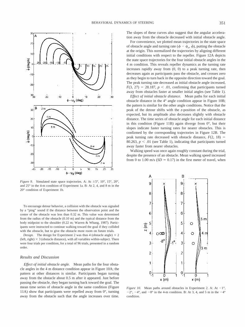
Effect of initial obstacle angle. Mean paths for the four obsta-cle angles in the 4 m distance condition appear in Figure 10A; thepattern at other distances is similar. Participants began turningaway from the obstacle about 0.5 m after it appeared. Just beforepassing the obstacle, they began turning back toward the goal. Themean time series of obstacle angle in the same condition (Figure11A) show that participants were repelled away from 0°, turningaway from the obstacle such that the angle increases over time.

The slopes of these curves also suggest that the angular accelera-tion away from the obstacle decreased with initial obstacle angle.

For convenience, we plotted mean trajectories in the state spaceof obstacle angle and turning rate (� � �o, �), putting the obstacleat the origin. This normalized the trajectories by aligning differentinitial conditions with respect to the repeller. Figure 12A depictsthe state space trajectories for the four initial obstacle angles in the4 m condition. This reveals repeller dynamics as the turning rateincreases rapidly away from (0, 0) to a peak turning rate, thendecreases again as participants pass the obstacle, and crosses zeroas they begin to turn back in the opposite direction toward the goal.The peak turning rate decreased as initial obstacle angle increased,F(3, 27) � 28.187, p .01, confirming that participants turnedaway from obstacles faster at smaller initial angles (see Table 1).

Effect of initial obstacle distance. Mean paths for each initialobstacle distance in the 4° angle condition appear in Figure 10B;the pattern is similar for the other angle conditions. Notice that thepeak of the detour shifts with the z-position of the obstacle, asexpected, but its amplitude also decreases slightly with obstacledistance. The time series of obstacle angle for each initial distancein this condition (Figure 11B) again diverge from 0°, but theirslopes indicate faster turning rates for nearer obstacles. This isconfirmed by the corresponding trajectories in Figure 12B. Thepeak turning rate decreased with obstacle distance, F(2, 18) �80.263, p .01 (see Table 1), indicating that participants turnedaway faster from nearer obstacles.

Walking speed was once again roughly constant during the trial,despite the presence of an obstacle. Mean walking speed increasedfrom 0 to 1.00 m/s (SD � 0.17) in the first meter of travel, when

Figure 10. Mean paths around obstacles in Experiment 2. A: At �1°,�2°, �4°, and �8° in the 4-m condition. B: At 3, 4, and 5 m in the �4°condition.

Figure 9. Simulated state space trajectories. A: At �5°, 10°, 15°, 20°,and 25° in the 4-m condition of Experiment 1a. B: At 2, 4, and 8 m in the20° condition of Experiment 1b.


the obstacle appeared. Mean maximum walking speed was 1.21m/s (SD � 0.17), which decreased to 0.08 m/s (SD � 0.02) in thelast second before contact with the goal. Initial and final walkingspeed were unaffected by initial obstacle angle and distance.Maximum walking speed was unaffected by initial obstacle angle,but it increased slightly with initial obstacle distance (1.19, 1.21,and 1.23 m/s for 3, 4, and 5 m, respectively).

These results demonstrate that initial obstacle angle and distanceinfluence turning away from an obstacle. The angular accelerationdecreases with obstacle angle—it did not decrease with goal anglein Experiment 1—but it also decreases with obstacle distance, asit did with goal distance in Experiment 1. This is again consistentwith efficient obstacle avoidance. If the angular acceleration werenot affected by the obstacle angle and distance, then observerswould risk colliding with nearby obstacles in their path, or theymight generate unnecessary torque to avoid distant obstacles orthose at large angles. Thus, having angular acceleration depend onobstacle angle and distance ensures effective obstacle avoidanceunder a variety of conditions.

We can summarize our findings thus far as follows: Angularacceleration increases with goal angle and decreases with goaldistance, whereas it decreases with both obstacle angle and obsta-cle distance.

Obstacle component of the model. On the basis of the resultsof Experiment 2, we extended the model by adding an obstaclecomponent:

� � �b� � kg �� g��e�c1dg � c2�

� ko �� o��e�c3�� o��e�c4do�, (12)

where ko, c3, and c4 are obstacle parameters. First, the obstacle“stiffness” term ko (� � �o)(e

�c1��o�) reflects the finding that theangular acceleration away from an obstacle decreases with obsta-cle angle. We modeled this with an exponential function that risessharply from a heading of 0° to a peak close to the obstacle andthen asymptotes to near zero (Figure 2B); the spread of thisfunction is determined by parameter c3, which has units of 1/rad.When heading to the right of an obstacle, this induces a positiveacceleration away from the obstacle to the right; when heading tothe left of the obstacle, the reflection of this function induces anegative acceleration to the left. Second, analogous to the goalcomponent, the distance term �e�c4do) reflects the finding that theturning rate away from an obstacle decreases exponentially withobstacle distance. It acts to modulate the parameter ko, so that the

Figure 12. Trajectories in the state space of turning rate (�) by obstacleangle (� � �o) in Experiment 2. A: At 1°, 2°, 4°, and 8° in the 4-mcondition. B: At 3, 4, and 5 m in the 4° condition.

Figure 11. Mean obstacle angle time series in Experiment 2. A: At 1°, 2°,4°, and 8° in the 4-m condition. B: At 3, 4, and 5 m in the 4° condition.


amplitude of the function in Figure 2B, and hence the repulsion ofthe obstacle, decays with distance. Parameter c4 determines therate of decay with obstacle distance and has units of 1/m; in thiscase acceleration is allowed to asymptote to near zero as distanceincreases.

Using the parameter settings for b, kg, c1, and c2 from Experi-ment 1, we simulated the extended model under the conditions ofExperiment 2 to identify the values for ko, c3, and c4 that best fitthe mean obstacle angle time series, using a least-squares proce-dure. Only the portion of the obstacle angle time series before theobserver passed the obstacle was used to evaluate the fit (i.e.,before the observer’s z-coordinate became greater than the obsta-cle’s z-coordinate). The best mean fit (r2 � .975) was found withvalues of kg � 198.0, c3 � 6.5, and c4 � 0.8. Simulation results forthe time series of obstacle angle appear in Figure 13, whichillustrates that the model reproduces the effects of obstacle angleand distance observed in human behavior (compare Figure 11).Some curves are slightly less bowed, indicating that the modelveers away from nearby obstacles sooner than human participants.Trajectories for the model demonstrate that the peak turning ratedecreases with initial obstacle angle (Figure 14A) and with initial

obstacle distance (Figure 14B). These trajectories are similar tothose for participants in Figure 12, although the model reachessomewhat higher peak velocities. Nevertheless, the model success-fully reproduces both key features of Experiment 2 and provides agood quantitative fit to the human data.

Experiment 3: Route Selection With One Obstacle

Up to this point, we have only considered steering behavior withrespect to a single goal or obstacle. In natural environments,however, configurations of objects often require observers to selecta particular route to a goal from among different possible pathsthrough an array of obstacles. The simplest case involves adoptingone of two possible routes around an obstacle that lies between theobserver’s initial heading direction and the direction of the goal(see Figure 1). In this case, the observer could take either anoutside (left) or an inside (right) path around the obstacle to reachthe goal. What determines the actual route that the observeradopts?

A common approach to path planning is model-based control,which is characterized in robotics by a “sense-model-plan-act”scheme (Brooks, 1991; Moravec, 1981). Sensory information isused to construct an internal model of the environment, whichrepresents the detailed 3-D layout of objects and surfaces in thescene. An action path is then explicitly planned on the basis of thismodel before being executed in the real world. For example, a pathplanning process might generate a route by determining the short-est distance to the goal or by following a minimum energy paththrough a landscape of potential “hills” corresponding to thelocations of obstacles (Khatib, 1986).

An alternative approach, which Warren (1998) called information-based control, was anticipated by Gibson (1958/1998) and hasbeen promoted in behavior-based robotics (Brooks, 1991; Duchon,Warren, & Kaelbling, 1998; Meyer & Wilson, 1991). In this case,available information is used to govern behavior in an on-linemanner. The path adopted by the agent is not planned in advance;rather, it emerges as a consequence of the control laws by whichinformation modulates action. Because occurrent information reg-ulates control variables directly, an internal model of the environ-ment and explicit path planning become unnecessary. What ap-pears to be planned sequential behavior can thus emerge from thedynamic interaction between agent and environment, rather thanimplicating an action plan.

It is precisely this interaction that is captured in our model of thebehavioral dynamics of steering and obstacle avoidance. The aimof Experiment 3 was to see whether the simplest case of humanroute selection could be accounted for by the model in terms ofon-line steering dynamics, without recourse to explicit path plan-ning. Note that this is not a critical test of the two approaches, butrather a demonstration of the sufficiency of a more parsimoniousinformation-based approach.

In the present experiment, we recorded the routes taken byhuman participants around an obstacle to a goal, when the obstaclewas located between the initial heading direction and the goaldirection (Figure 1). We varied the initial distance of the goal (dg)and the offset angle between the goal and the obstacle (�g � �o),to determine the conditions under which people switch froman outside to an inside path. We then tested whether the modelpredicted the observed routes, using the parameter values de-

Figure 13. Simulated obstacle angle time series in Experiment 2. A: At1°, 2°, 4°, and 8° in the 4-m condition. B: At 3, 4, and 5 m in the 4°condition.


rived in Experiments 1 and 2. To the extent that the model canreproduce the human paths, this would suggest that it is possible inprinciple to account for human route selection in terms of thedynamics of elementary behaviors for steering and obstacleavoidance.

Method

Participants. Ten undergraduate and graduate students, 4 women and6 men who ranged in age from 18 to 26 years, participated in Experiment3. None reported having any visual or motor impairment. They were paid$6 for their participation.

Stimuli. As in the previous experiments, participants began walkingtoward the distant marker when it turned green. After traveling 0.5 m, themarkers disappeared and participants continued walking and looking in thesame direction. After another 0.5 m, a blue goal post and a red obstacleappeared simultaneously on the left or right of the participant’s path, withthe obstacle in between the heading direction and the goal direction (referto Figure 1A). First, we manipulated the initial offset angle between theobstacle and the goal (�g � �o � 1°, 2°, 4°, or 8°) by holding the initialgoal angle constant (� � �g � 15°) and varying the initial obstacle angle(� � �o � 14°, 13°, 11°, 7°). Second, we manipulated the initial goaldistance (dg � 5, 7, or 9 m) while holding the initial obstacle distance

constant (do � 4 m). Participants were instructed to walk to the goal whileavoiding the obstacle along the way, and they were told that they couldpass to either side of the obstacle. As in Experiment 2, a collision with theobstacle was signaled by a “ping” if the point of observation came closerthan 0.32 m to the center of the obstacle.

Design. The experiment had a 4 (offset angle) � 2 (left, right) � 3(goal distance) factorial design, with all variables within-subject. Therewere four trials per condition, resulting in a total of 96 trials presented ina random order.


Mean paths for each initial offset angle (different panels) andinitial goal distance (different curves) appear in Figure 15A, col-lapsed so all objects appear on the right of the initial heading. Themost frequently selected route for each condition is represented bythe solid curve. Participants took both inside and outside paths tothe goal in nearly all conditions. However, as shown in Figure15C, the distribution of paths shifted systematically across condi-tions, such that the percentage of inside paths increased with theoffset angle and the nearness of the goal. On average, participantsswitched from an outside path to an inside path at an offset anglesbetween 2° and 4°, and they were more likely to do so when thegoal was nearer. A two-way analysis of variance on the percentageof inside paths revealed significant main effects of offset angle,F(3, 27) � 94.83, p .01, and goal distance, F(2, 18) � 53.46,p .01, with no interaction, F(6, 54) � 1.17, p � .34. Insummary, participants were more likely to switch from an outsideto an inside path as offset angle increased and goal distancedecreased. This confirms the necessity of including an explicitterm for goal distance in the model.

Simulations. We tested the model on scene configurationssimilar to those in Experiment 3. The initial goal distance variedbetween 5 and 9 m, and the initial offset angle between 1° and 15°,while the initial goal angle (15°) and initial obstacle distance (4 m)were held constant. Our first set of simulations used parametervalues determined from Experiment 1b for the goal component andExperiment 2 for the obstacle component, as before. The modelsuccessfully predicts the shift from outside to inside paths withlarger offset angles and nearer goals. Specifically, it generatesan outside path for offset angles � 7° and an inside path forangles � 10°. Between 7° and 10°, the model takes an outside pathwith larger goal distances and switches to an inside path withsmaller goal distances, replicating the qualitative pattern of humanroutes.

The shift to inside paths, however, occurred at somewhat largeroffset angles for the model (7–10°) than for human participants(2–4°). Thus, using parameter settings based on Experiments 1 and2, the model is somewhat biased toward outside paths. One reasonfor this may be that the first two experiments sampled a limitedrange of conditions, and in particular they did not include cases inwhich participants crossed in front of the obstacle to reach thegoal. It is possible that participants adapted their behavior (ad-justed their “parameters”) to these conditions, so the parameter fitsdid not generalize precisely to a wider range of conditions. Wethus performed a second set of simulations to determine whetherwe could reproduce the pattern of routes observed in Experiment3 with a minimal change in parameter values. Adjusting a singleparameter, c4, from 0.8 to 1.6, was sufficient to induce the shiftfrom an outside to an inside path at offset angles of 1° to 4° (see

Figure 14. Simulated state space trajectories in Experiment 2. A: At 1°,2°, 4°, and 8° in the 4-m condition. B: At 3, 4, and 5 m in the 4° condition.


Figure 15B). This increased the decay rate of obstacle repulsionwith distance, allowing closer approaches to obstacles, and thus c4

might be thought of as a “risk” parameter.In these simulations, the effect of initial goal distance is a

consequence of the fact that the attractive strength of the goal, andhence angular acceleration toward it, increase for nearer goals. Theeffect of offset angle is a consequence of the trade-off betweenthe attractive strength of the goal, which increases with angle, andthe repulsive strength of the obstacle, which decreases with angle.Initially, the goal component dominates, turning the agent in thedirection of the goal. However, the resulting decline in both goaland obstacle angles reduces the attractive strength of the goalwhile increasing the repulsive strength of the obstacle. Whether theagent follows an inside or outside path depends on which compo-

nent dominates as the agent heads toward the obstacle. For smalloffset angles, illustrated in Figure 16A–B, the goal angle is rela-tively small as the agent turns toward the obstacle. Hence, obstaclerepulsion overcomes goal attraction, forcing the agent onto anoutside path. For large offset angles, in Figure 16C–D, the goalangle is larger as the agent turns toward the obstacle. Hence, goalattraction overcomes obstacle repulsion, drawing the agent onto aninside path. Thus, the observed route arises from competitionbetween goal attraction and obstacle repulsion in the behavioraldynamics.

Model dynamics. To gain a better understanding of the under-lying dynamics, we plotted vector fields at several positions ontypical inside and outside routes (see Figure 17). Each plot repre-sents the state space of heading (�) by turning rate (�) for one

Figure 15. Experiment 3 data. A: Mean paths in the 5-, 7-, and 9-m initial goal distance conditions for eachinitial goal-obstacle offset angle. Solid lines correspond to the most frequently selected route in each condition.B: Simulated paths with an initial offset angle of 2°, with parameter c4 � 1.6. C: Percentage of inside paths asa function of initial goal-obstacle offset angle for each condition of initial goal distance. D: Model simulationsof the percentage of inside paths, with 10% error in perceptual variables and parameters and variability in initialconditions matched to the human data.


position in the environment. The small vectors illustrate the flowof the system at each point in state space, the horizontal componentcorresponding to the change in X (angular velocity �) and thevertical component corresponding to the change in Y (angularacceleration �) at that point. The heavy line is the nullcline atwhich acceleration is zero and the vectors are purely horizontal. Itsintersections with the X-axis (the other nullcline, at which velocityis zero) identify the system’s fixed points.

Because the four-dimensional system is difficult to visualize(i.e., �, �, x, and z), we plot vector fields for a sequence of (x, z)positions to better understand how the dynamics change as theagent moves through this four-dimensional space. In Figure 17A,the goal is initially located at 15° and 7 m and the obstacle at 11°and 4 m from the agent’s starting position at (x, z) � (0, 0). In thecorresponding vector field (Figure 17B), there is a single attractorat (�, �) � (15.2°, 0°/s), near the goal direction of �g � 15.0°(filled arrow) on the other side from the obstacle (open arrow).Although the location of the attractor is determined by the com-bination of the goal and obstacle components, the goal componentdominates at this point because the goal angle is large and theobstacle is distant, so the attractor is located near the goaldirection.

In Figure 17C, when the agent is to the left of the obstacle at (x,z) � (0.4, 3.2), the goal and obstacle components interact consid-erably. The system is bistable, with attractors at (2.8°, 0°/s) and(46.3°, 0°/s), separated by a saddle point at (27.1°, 0°/s). The formof this shift from one- to two-point attractors is analogous to a

tangent bifurcation in a first-order system (Strogatz, 1994). Thebistability means that the agent may accelerate either to the left orright of �g � 21.6°, depending on the current heading and turningrate. Note that although the two attractors lie to the left and rightof the obstacle at �o � 26.6°, they do not necessarily yield outsideand inside paths, respectively. Because the vector field changes asthe agent’s (x, z) position changes, the location and number ofattractors change as well.

In Figure 17D, the agent is passing to the right of the obstacleat (x, z) � (1, 3) and there is a single attractor at (19.2°, 0°/s). Theattractor is located slightly to the right of the goal at �g � 12.2°because the obstacle at �o � �14.3° still exerts an influence,pushing the agent slightly to the right of the goal and well awayfrom the obstacle. After the agent is past the obstacle at (x, z) �(1.25, 5.0) in Figure 17E, the obstacle exerts no influence and thereis a single attractor at (24.0°, 0°/s), in the same direction as thegoal at �g � 24.0°. Thus, the attractor locations are determined bythe competition between goal and obstacle components. Where theobstacle component is weak, there is only a single attractor nearthe goal direction. Where the obstacle component is strong, morethan one attractor may exist and none is aligned with the goal. Inthis way the attractor landscape evolves as the agent movesthrough the environment, and its behavior is structured by bothattractors and repellers.

Perceptual and parameter error. It is apparent from Figure 15that there was some variation in human routes that is not repro-duced by the model, as indicated by the distribution of paths on

Figure 16. Plots of changing contributions of goal and obstacle components for a sample outside route witha 1° offset angle (A, B) and inside route with an 8° offset angle (C, D). In A and C, black circles along pathsrepresent 1-s time intervals, and black crosses represent the goal. In B and D, solid lines correspond to goalcomponent, and dotted lines correspond to obstacle component. Positive acceleration is in the clockwisedirection, and negative acceleration is in the counterclockwise direction.


either side of the obstacle. This might be captured by the intro-duction of variable error in perceptual variables (i.e., goal andobstacle angle and distance) and parameters. At the same time, itis important to determine whether the model is reasonably robustto such error. We investigated the robustness issue by addingvariability to each perceptual variable and each parameter, both

individually and in various combinations, for selected configura-tions used in Experiments 1 and 2. On each simulated trial, an errorconstant was randomly selected for each perceptual variable orparameter from a Gaussian distribution with a mean of 1.0 and astandard deviation of 0.1. Variable error was added to the modelby multiplying the actual value of each perceptual variable or

Figure 17. A: Vector fields (� vs. �) at four points along typical outside and inside routes. B–E: For smallvectors, the vertical component represents angular acceleration (�), and the horizontal component representsangular velocity (�). Solid curves represent nullclines at which � is zero. Filled circles represent point attractors,and empty circles represent repellers. Filled arrows indicate the goal direction (�g), and open arrows indicate theobstacle direction (�o).


parameter by the corresponding error constant. For the Experiment1 configuration, initial goal angle was 20° and initial goal distancewas 4 m. For the Experiment 2 configuration, initial obstacle anglewas �4° and initial obstacle distance was 4 m. The effect of errorwas measured by taking the standard deviation of the x-coordinatehalfway through the trial (Experiment 1 configuration) or when thez-coordinate equaled that of the obstacle (Experiment 2 configu-ration). The results, based on 1,000 simulations for each perceptualvariable or parameter (or combination), using 10% error are sum-marized in Table 2. Parameter error yielded slightly more variabil-ity than perceptual error, but in all cases the model tolerated bothtypes of error quite well. Even when 10% error was added to allperceptual variables and parameters at the same time, the standarddeviation of x-position was only 4.15 cm in the Experiment 1configuration and 11.55 cm in the Experiment 2 configuration.

We then determined whether the distribution of human pathsobserved in Experiment 3 could be reproduced by introducingvariable error. We simulated the model under the same conditionsused in Experiment 3, adding 10% error to each perceptual vari-able and parameter. We also randomly varied the initial x-positionand heading on each simulated trial, matching the standard devi-ation to the mean standard deviation observed in Experiment 3(SD � 0.16 cm for initial x-position and SD � 6.58° for initialheading). The percentage of inside paths is plotted as a function ofinitial offset angle for each initial goal distance in Figure 15D.Comparing the simulations to the human data in Figure 15C, it isclear that the observed distribution of paths can be effectivelyreproduced by adding variable error to the model and matching theinitial conditions.

Thus, the model can predict the qualitative behavior of humanroute selection using parameter settings from Experiments 1 and 2,

and it can reproduce those routes quantitatively with an adjustmentin a single “risk” parameter. Furthermore, the distribution ofhuman paths is captured by the addition of 10% perceptual andparameter error in the model and variation in initial conditions.This pattern of results demonstrates that simple route selection canbe accounted for in terms of elementary behavioral components forsteering and obstacle avoidance.

General Discussion

In the research we report here, we sought to derive a model ofthe behavioral dynamics of human steering and obstacle avoidanceand use it to predict route selection in simple scenes. In the firstexperiment, we collected descriptive data on walking toward agoal and found that steering exhibited point attractor dynamics thatdepended on initial goal angle and distance. In the second exper-iment, similar data on obstacle avoidance revealed repeller dynam-ics that also depended on initial obstacle angle and distance. Wemodeled the steering dynamics as a linear combination of a goalterm and an obstacle term. The attraction of the goal increasedlinearly with its angle from the current heading and decreasedexponentially with distance, whereas the repulsion of the obstacledecreased exponentially with angle and with distance. In the lastexperiment, we used the model to predict route selection in thesimplest case of steering to the left or right of an obstacle. Param-eter settings derived from the first two experiments generated thequalitative pattern of routes, and an adjustment in one “risk”parameter reproduced them quantitatively. Steering behavior, ob-stacle avoidance, and route selection thus emerge from a systemthat simply follows locally specified attractors.

We believe the contributions of this work are threefold. First,the results provide the first parametric data of which we are awareon the fundamental human behavior of walking to goals andavoiding obstacles. Second, the model represents the extension ofa dynamical systems analysis from simple laboratory tasks withstationary dynamics to complex behavior whose dynamics dependon the interaction between the agent and the environment. Third,the results provide the first demonstration we know of that not onlyattractors but also repellers serve to structure behavior in biolog-ical systems, analogous to the work of Schoner et al. (1995) inrobotics.

Regarding the human data, several basic observations can bemade. First, people make gradual turns during walking, changingtheir heading direction over several steps rather than pivoting onone foot to abruptly switch directions, thereby mitigating theinertial effects of changing direction. On the other hand, they donot travel on a continuous arc to the goal, but turn onto anapproximately linear path that aligns their heading direction withthe goal. This is consistent with the idea that, at least in open fieldwalking, people control their current heading so that it is alignedwith the goal, and it is contrary to theories that suggest peoplefollow curved paths to a target (Lee, 1998; Wann & Swapp, 2000).Second, the rate of turning is influenced by both the distance of agoal or obstacle and its angle with respect to the heading direction.Turning is thus not a biomechanically stereotyped act but appearsto be governed by information about the observer’s movementrelative to objects in the scene.

Table 2Effects of 10% Perceptual and Parameter Errorsin Experiment 1 and 2 Configurations

Source of error

SD of x-position

Experiment 1 Experiment 2

Perceptual variables

Goal angle 1.51 1.26Goal distance 1.78 1.21Obstacle angle 4.39Obstacle distance 3.82All 2.06 6.63

Parameters

b 2.52 2.56kg 2.79 2.90c1 1.74 1.17c2 1.98 2.41ko 2.39c3 6.89c4 4.13All 4.05 9.44

Perceptual variables and parameters

All 4.15 11.55


Dynamics of Steering and Obstacle Avoidance

The model itself can be evaluated in two ways: as a descriptivemodel of the behavioral dynamics of steering and obstacle avoid-ance and as a predictive model of route selection. In the firstinstance, we believe the model does a good job of capturing thebehavioral dynamics. It compactly describes the behavior of steer-ing toward a goal or around an obstacle with fits near r2 � 1.0. Thelinear combination or superposition of goal and obstacle terms isadvantageous because the model scales linearly with the complex-ity of the scene, adding a term for each new object (Large,Christensen, & Bajcsy, 1999). In practice, the model is even moreefficient, because it only depends on information about objects thatappear within a restricted zone in depth and about the currentheading. Specifically, the obstacle component decreases to nearzero at a distance of about 4 m and an angle of �60° from theheading direction (Figure 2B). This implies that human steeringbehavior is not based on the complete 3-D layout of the scene, buton a limited sample of the next few objects near the path of travel.Such a result is consistent with use of on-line information forsteering control, rendering a detailed internal world model andexplicit path planning unnecessary.

Another type of internal representation often thought to benecessary for control is a model of the plant dynamics (Loomis &Beall, 1998). Such a model of the relationship between controlvariables and resulting body movements would allow the agent topredict future states of the body. However, if behavior is a con-sequence of laws of control and physical constraints, an explicitmodel of the plant dynamics is unnecessary. Instead, the agentmight simply learn parameter settings for the control law that yieldsuccessful behavior within the given physical constraints. If theseconstraints change (e.g., if the agent’s mass increases or themedium changes from air to water), the agent may adapt by tuningthe parameters to stabilize behavior again. Thus, the agent’s“model” of the plant dynamics is simply a set of parameter valuesthat result in successful behavior within given constraints.

Route Selection

We also believe that the model is a promising first account ofroute selection. By fitting the model to human data from thelimited conditions of Experiments 1b and 2, we were able topredict the qualitative pattern of routes observed in the simple casein Experiment 3. It is likely that fitting the model to data frommore general conditions would allow us to make more quantitativepredictions. Thus, our current research fixes parameters on thebasis of Experiment 3 and attempts to predict human routesthrough more complex scenes by linearly combining terms forgoals and obstacles, including pairs of obstacles, random arrays ofobstacles, and cul-de-sacs (Fajen, Beem, & Warren, 2002).

The main limitation of the model is that it currently representsobstacles as points. This is unrealistic for complex scenes thatcontain wide obstacles or extended surfaces such as walls. Suchobjects might be represented in the model either by adjusting thedecay rate of the repulsion function (parameter c3 in Equation 12;see Figure 2B), or by treating a wide obstacle as a set of points atfinite intervals and summing their influence. The latter predictsthat people turn away from wide obstacles faster than from smallones. The effects of obstacle width on steering behavior and route

selection remain to be empirically investigated. On the other hand,body width is implicitly represented in the model by the “risk”parameter c4, the decay rate of repulsion with distance (Warren &Whang, 1987).

A next step is to generalize the model from stationary goals andobstacles to moving goals and obstacles. In recent experiments, wefound that humans intercept moving targets by seeking to achievea constant angle between the target and the heading (Fajen &Warren, 2002). This can be incorporated in the model by adding aterm to the goal angle that depends on the angular velocity of thetarget (�g), so as to shift the attractor ahead of the target by anamount proportional to target speed. A similar term might beinserted into the obstacle component to avoid moving obstacles.When the steering model for an individual agent is complete, itwould allow us to simulate the behavior of multiple interactingagents in a dynamic environment, including crowd behavior.

The present results demonstrate that it is possible, in principle,to account for human route selection as a consequence of elemen-tary behaviors for steering and obstacle avoidance. In effect, theagent adopts a particular route through the scene on the basis oflocal responses to visually specified goals and obstacles. Theobserved route is not determined in advance through explicitplanning, but rather emerges in an on-line manner from the agent’sinteractions with the environment. It is possible, of course, todevelop an off-line path planning account of the results fromExperiment 3; the model simply demonstrates that a more parsi-monious on-line account is plausible and adequate to the data. It isalso possible that familiarity with the layout of goals and obstacleswould influence route selection in a manner that cannot be cap-tured by the model in its current form. We are currently investi-gating how route selection changes with experience and consider-ing ways of expanding the model to accommodate these changes.Such changes might simply be captured by the tuning of param-eters in the model.

Behavioral Dynamics and Control Laws

The present model differs from the robotic control model ofSchoner et al. (1995) in two closely related ways. First, because itdescribes the observed behavior of an inertial agent, we wereforced to abandon a first-order system and adopt a higher-ordersystem. Second, our model treats steering adjustments as transientbehavior en route to a stable attractor (heading in the goal direc-tion). In contrast, Schoner et al.’s model is a first-order system thatis at all times in an attractor state and thus stable at every moment.The significance of such a first-order model is that it permits theintegration of multiple constraints (goals and obstacles in arbitrarypositions) in such a way that a solution can be assured, guaran-teeing that the observer does not collide with an obstacle, becometrapped in a local minimum, oscillate between two goals, or notreach the goal. In contrast, there is no way to ensure that transientsolutions satisfy multiple arbitrary constraints. These differencesfollow directly from Schoner et al.’s modeling of a control systemat the first level of analysis, whereas we modeled the behavioraldynamics of a physical agent at the second level of analysis.First-order control laws may be advantageous to achieve well-behaved solutions under multiple constraints. At the same time,observed behavior is a consequence of these control laws interact-ing with the physics of the body and environment and thus requires


a higher-order description. As outlined in the introduction, wesuggest that these two levels of analysis, and hence the twomodels, are complementary. Now that we have a formal descrip-tion of the behavioral dynamics of steering, we can considerwhether a first-order control law can give rise to this behavior.

Let us assume that a first-order control law is embedded withina second-order system representing the physical body. The form ofthe control law can be borrowed from the terms in our model,which capture the behavioral influence of goals and obstacles:

� � �kg �� g��e�c1dg � c2� � ko �� o�

� �e�c3��o�)(e�c4do�. (13)

This control law is a dynamical system that takes the visuallyspecified current heading, goal angle and distance, and obstacleangles and distances, and immediately relaxes to an attractor forthe intended heading at a value �*. A prime has been added to theangular acceleration (�) to distinguish the control law from phys-ical acceleration of the body. Note that �* is determined by thecombination of goal and obstacle terms, and it may not necessarilycorrespond to the direction of the goal. Given the intended head-ing, the angular acceleration of the body is then determined by asecond-order system, whose parameters are independent of thelayout of goals and obstacles in the world:

� � �bb� � kb �� *�. (14)

Because of the body’s inertia, the resulting behavior has a slowerrelaxation time than the control law, so the actual heading lagsbehind the intended heading. Thus, whereas the control law tracksa stable attractor, the observed behavior is transient. Note that thisconcept of a control law as a dynamical system is distinct fromconceiving of it as a simple mapping from an optical variable to anaction variable.

In simulations performed by Philip Fink (a postdoctoral researchassociate in the VENLab), we tested this embedded model with agoal and one obstacle, under the conditions of Experiment 2. Meanpaths were nearly identical to those of the higher order model, andleast-squares fits to the mean time series of goal angle had a meanr2 � .991. The resulting parameter values, which were naturallydifferent from the higher order model, were kg � 59.1625, c1 �0.0555, c2 � 0.01125, ko � 842, c3 � 2.74063, c4 � 0.04653,bb � .0375, and kb � 592. Thus, the higher order behavioraldynamics that we observed experimentally can be accounted for interms of a first-order control system, preserving the advantages ofa stable solution that satisfies multiple constraints. These resultsdemonstrate that the behavior of steering and obstacle avoidancecan be modeled consistently at two levels, the first involvinginteractions between a first-order control law and the physics ofthe body and world, and the second providing a higher orderdescription of the emergent behavior.

It is important to show that the informational variables in thecontrol law are perceptually available. Although we parameterizedthe model in terms of object distance, the control law might bebased on either the perceived distance of the object or the per-ceived time-to-contact specified by the optical variable (Bootsma& Craig, 2002; Lee, 1980). Given that the influence of obstaclesgradually asymptotes to zero around 4 m and the influence of thegoal to a constant value beyond 8 m, accurate perception of

distance or time-to-contact is not essential. With time-to-contactless than 4 s, obstacles are within the range of sensitivity to (Schiff & Detwiler, 1979), and given that the control process iscontinuous accuracy improves as an obstacle is approached.

Goal and obstacle angles are also perceptually specified. Warrenet al. (2001) found that walking is guided by a combination of thevisual direction of the goal with respect to the heading specified byoptic flow ��flow � �g�, and the egocentric direction of the goalwith respect to the locomotor axis, which is presumably specifiedproprioceptively ��loco � �g�. Thus, we can expand the infor-mational term in the goal component of the control law as

� � �g � �� loco � �g� � wv ��flow � �g�, (15)

where v is observer velocity and w represents environmentalstructure, both of which influence the magnitude and area of opticflow. It remains to be empirically determined whether the obstaclecomponent can be similarly expanded.

Comparison With Other Models

Our dynamical model bears a resemblance to potential fieldmodels of path planning (Khatib, 1986), which also representbehavior as transients to attractor states. However, in comparativesimulations of the two models, we observed some notable differ-ences (see Fajen, Warren, Temizer, & Kaelbling, in press, fordetails). First, in the potential field approach the attractors andrepellers are defined as the two-dimensional positions of goals andobstacles in the world, whereas the dynamical approach definesthem as values of the behavioral variables (heading and turningrate). Thus, whereas behavior is determined by the agent’s positionin the potential field model, behavior in our dynamical model isdetermined by the agent’s position, heading, and turning rate.Second, whereas potential field models control translation direc-tion, the present dynamical model determines angular accelerationand thus tends to yield smoother trajectories. Third, as a conse-quence of acceleration, our dynamical model can produce differentpaths for different translation speeds. In contrast, because thepotential field equations determine the direction of the agent’smotion from its position, it always traverses the same path regard-less of speed. Finally, comparative simulations reveal that thedynamical model generates markedly smoother and shorter pathsto the goal and that local minima can be avoided by reducing thedecay rate of the “risk” parameter c4.

We should point out that the observed human paths departdramatically from a simple shortest path criterion (see particularlyFigure 15). To our knowledge, no other models have been pro-posed for locomotor paths that take obstacle avoidance into ac-count. Note that the present model does not incorporate an explicitoptimality principle, although its form or parameter values couldresult from such principles over the course of evolution or learn-ing, such as a combination of minimizing energy and injury.

Conclusion

In summary, the present model captures the behavioral dynam-ics of human steering and obstacle avoidance with good fidelity,and it can reproduce the pattern of routes through a simple scene.This suggests that human route selection does not require explicitplanning but may emerge on-line as a consequence of elementary


behaviors for steering and obstacle avoidance. We are currentlyinvestigating whether the present form of the model can alsoaccount for route selection in more complex scenes.

References

Bootsma, R. J., & Craig, C. M. (2002). Global and local contributions tothe optical specification of time to contact: Observer sensitivity andcomposite tau. Perception, 31, 901–924.

Brooks, R. A. (1991). Intelligence without representation. Artificial Intel-ligence, 47, 139–160.

Collins, J. J., & Stewart, I. (1993). Hexapodal gaits and coupled nonlinearoscillator models. Biological Cybernetics, 68, 287–298.

Diedrich, F. J., & Warren, W. H. (1995). Why change gaits? Dynamics ofthe walk-run transition. Journal of Experimental Psychology: HumanPerception and Performance, 21, 183–202.

Duchon, A. P., & Warren, W. H. (2002). A visual equalization strategy forlocomotor control: Of honeybees, robots, and humans. PsychologicalScience, 13, 272–278.

Duchon, A. P., Warren, W. H., & Kaelbling, L. P. (1998). Ecologicalrobotics. Adaptive Behavior, 6, 473–507.

Fajen, B. R. (2001). Steering toward a goal by equalizing taus. Journal ofExperimental Psychology: Human Perception and Performance, 27,953–968.

Fajen, B. R., Beem, N., & Warren, W. H. (2002, May). Route selectionemerges from the dynamics of steering and obstacle avoidance. Paperpresented at the 2nd Annual Conference of the Vision Sciences Society,Sarasota, FL.

Fajen, B. R., & Warren, W. H. (2002). Intercepting a moving target onfoot. Manuscript submitted for publication.

Fajen, B. R., Warren, W. H., Temizer, S., & Kaelbling, L. P. (in press). Adynamical model of visually-guided steering, obstacle avoidance, androute selection. International Journal of Computer Vision.

Gibson, J. J. (1979). The ecological approach to visual perception. Boston:Houghton Mifflin.

Gibson, J. J. (1998). Visually controlled locomotion and visual orientationin animals. Ecological Psychology, 10, 161–176. (Reprinted from Brit-ish Journal of Psychology, 49, 182–194, 1958)

Jeka, J. J., Kelso, J. A. S., & Kiemel, T. (1993). Spontaneous transitionsand symmetry: Pattern dynamics in human four-limb coordination. Hu-man Movement Science, 12, 627–651.

Kay, B. A., & Warren, W. H. (2001). Coupling of posture and gait: Modelocking and parametric excitation. Biological Cybernetics, 85, 89–106.

Kelso, J. A. S. (1995). Dynamic patterns: The self-organization of brainand behavior. Cambridge, MA: MIT Press.

Khatib, O. (1986). Real-time obstacle avoidance for manipulators andmobile robots. International Journal of Robotics Research, 5, 90–98.

Kugler, P. N., & Turvey, M. T. (1987). Information, natural law, and theself-assembly of rhythmic movement. Hillsdale, NJ: Erlbaum.

Land, M. (1998). The visual control of steering. In L. R. Harris & H.Jenkins (Eds.), Vision and action (pp. 163–180). New York: CambridgeUniversity Press.

Large, E. W., Christensen, H. I., & Bajcsy, R. (1999). Scaling the dynamic

approach to path planning and control: Competition among behavioralconstraints. International Journal of Robotics Research, 18, 37–58.

Lee, D. N. (1980). Visuo-motor coordination in space-time. In G. E.Stelmach & J. Requin (Eds.), Tutorials in motor behavior (pp. 281–295).Amsterdam: North-Holland.

Lee, D. N. (1998). Guiding movement by coupling taus. Ecological Psy-chology, 10, 221–250.

Li, L., & Warren, W. H. (2002). Retinal flow is sufficient for steeringduring simulated rotation. Psychological Science, 13, 485–491.

Loomis, J. M., & Beall, A. C. (1998). Visually controlled locomotion: Itsdependence on optic flow, 3-D space perception, and cognition. Eco-logical Psychology, 10, 271–285.

Meyer, J. A., & Wilson, S. W. (Eds.). (1991). From animals to animats.Cambridge, MA: MIT Press.

Moravec, H. P. (1981, August). Obstacle avoidance and navigation in thereal world by a seeing robot rover. Proceedings of the 7th InternationalJoint Conference on Artificial Intelligence, Los Altos, CA.

Reichardt, W., & Poggio, T. (1976). Visual control of orientation behaviorin the fly: I. A quantitative analysis. Quarterly Review of Biophysics, 9,311–375.

Rushton, S. K., Harris, J. M., Lloyd, M., & Wann, J. P. (1998). Guidanceof locomotion on foot uses perceived target location rather than opticflow. Current Biology, 8, 1191–1194.

Schiff, W., & Detwiler, M. L. (1979). Information used in judging im-pending collision. Perception, 8, 647–658.

Schoner, G., & Dose, M. (1992). A dynamical systems approach totask-level system integration used to plan and control autonomousvehicle motion. Robotics and Autonomous Systems, 10, 253–267.

Schoner, G., Dose, M., & Engels, C. (1995). Dynamics of behavior: Theoryand applications for autonomous robot architectures. Robotics and Au-tonomous Systems, 16, 213–245.

Schoner, G., Jiang, W. Y., & Kelso, J. A. S. (1990). A synergetic theory ofquadrupedal gaits and gait transitions. Journal of Theoretical Biology,142, 359–391.

Strogatz, S. H. (1994). Nonlinear dynamics and chaos. Reading, MA:Addison-Wesley.

Wann, J. P., & Swapp, D. K. (2000). Why you should look where you aregoing. Nature Neuroscience, 3, 647–648.

Warren, W. H. (1988). Action modes and laws of control for the visualguidance of action. In O. Meijer & K. Roth (Eds.), Movement behavior:The motor-action controversy (pp. 339–380). Amsterdam: North-Holland.

Warren, W. H. (1998). Visually controlled locomotion: 40 years later.Ecological Psychology, 10, 177–219.

Warren, W. H. (2002). The dynamics of perception and action. Unpub-lished manuscript.

Warren, W. H. (in press). Optic flow. In L. Chalupa & J. S. Werner (Eds.),The visual neurosciences. Cambridge, MA: MIT Press.

Warren, W. H., Kay, B. A., Zosh, W. D., Duchon, A. P., & Sahuc, S.(2001). Optic flow is used to control human walking. Nature Neuro-science, 4, 213–216.

Warren, W. H., & Whang, S. (1987). Visual guidance of walking throughapertures: Body scaled information for affordances. Journal of Experi-mental Psychology: Human Perception and Performance, 13, 371–383.

(Appendix follows)


Appendix

Full Model Equations

The full model is given by the following equation:

� � � b� � kg �� g��e�c1dg � c2�

� �i�1

#obstacles

ko �� oi� e�c3��oi� �e�c4doi�. (A1)

Note that �g, dg, �o, and do change as the position of the agent changes (seeFigure 1A). However, each of these variables can be expressed as afunction of the (x, z) position of the observer:

�g � cos�1 � �Zg � z�

dg� , (A2)

dg � ��Xg � x�2 � �Zg � z�2�1/ 2, (A3)

�o � cos�1 � �Zo � z�

do� , (A4)

and

do � ��Xo � x�2 � �Zo � z�2�1/ 2, (A5)

where (Xg, Zg) and (Xo, Zo) are the coordinates of the goal and obstacle,respectively. Written as a system of first-order differential equations, themodel is given by the following:

y1 � �,

y2 � y1 � � � �by2 � kg �y1 � �g��e�c1dg � c2�

� �i�1

#obstacles

ko �y1 � �oi� e�c3�y1��oi� �e�c4doi�, (A6)

y3 � x � V sin y1,

y4 � z � V cos y1,

where V is the speed of the observer, which was held constant at 1 m/s inour simulations.

Received August 3, 2001Revision received May 24, 2002

Accepted August 27, 2002 �


Date post:	05-Dec-2021
Category:	Documents
Upload:	others
View:	3 times
Download:	0 times

Behavioral Dynamics of Steering, Obstacle Avoidance, and ...

Documents