Benchmarking Sparse Matrix-Vector Multiply inFive Minutes

Hormozd Gahvari, Mark Hoemmen, James Demmel, and Katherine YelickComputer Science Division

University of California, BerkeleyBerkeley, California 94720

Email: {hormozd,mhoemmen,demmel,yelick}@cs.berkeley.edu

Abstract— We present a benchmark for evaluating the perfor-mance of Sparse matrix-dense vector multiply (abbreviated asSpMV) on scalar uniprocessor machines. Though SpMV is animportant kernel in scientific computation, there are currentlyno adequate benchmarks for measuring its performance acrossmany platforms. Our work serves as a reliable predictor ofexpected SpMV performance across many platforms, and takesno more than five minutes to obtain its results.

I. INTRODUCTION

Sparse matrix-dense vector multiply (SpMV) is a commonoperation in scientific codes. It is especially prevalent initerative methods to solve linear systems. Given this, it wouldbe very convenient for consumers to have a convenient wayof knowing which machine to buy for their calculations, andfor vendors to know how well their machines perform.

There are currently no convenient ways for vendors to knowhow well their machines perform SpMV. The current standardmethod for ranking computers’ ability to perform scientificcompuatations, the Top 500 List [9], uses only the LINPACKbenchmark [8]. LINPACK measures the speed of solution ofa system of linear equations, which is not representative ofall the operations that are performed in scientific computing.There is a benchmark suite under development called the HighPerformance Computing Challenge Suite (HPCC) that seeksto remedy this [5]. The HPCC suite contains benchmarks thatseek to measure computers’ performance in performing severaldifferent operations, including LINPACK.

The benchmark we will present here is proposed for inclu-sion into this suite, as none of the other benchmarks in it aresuited for approximating the performance of SpMV. We willsee why in the next section. One requirement for inclusion inthe HPCC suite is a short run-time, which explains our goalof running in five minutes.

II. APPROXIMATING SPMV PERFORMANCE

A critical difference between SpMV and other operationsbenchmarked in the HPCC suite is that the performance ofSpMV depends strongly on the data, i.e. the size and nonzeropattern of the sparse matrix. Since practical sparse matricesdo vary widely in these properties, this means that existingbenchmarks will not be predictive of SpMV performance, andthat we will need to time SpMV itself on a representative setof test matrices.

Furthermore, as machines grow in capacity over time, nofixed set of test matrices would be adequate to test perfor-mance. For example, a matrix so large that it cannot be storedin cache on today’s platforms (an important size to test) maywell fit in cache in a few years. This would make SpMVappear to run at a much higher fraction of peak performance,and be unrepresentative of practical problem sizes, which willalso grow over time. This, combined with the sheer size ofa collection of fixed test matrices, means we will have togenerate appropriate test matrices on the fly that appropriatelyapproximate practical sparse matrices.

Finally, SpMV performance can vary significantly depend-ing on small changes in the data structure used to storethe matrix, and in the corresponding algorithm that accessesit to implement SpMV. Just as the LINPACK benchmarkdepends on tuned BLAS for a true assessment of a machine’sperformance, we also need to engage in a reasonable levelof tuning effort. To make this portable, fast and fair (in thesense that a similar level of machine-dependent and matrix-dependent tuning is done whenever the benchmark is used),we will rely on the OSKI automatic tuning system [11].

Now we explain the above points in more detail.The main reason different matrix sizes and nonzero patterns

impact the performance of SpMV is that they lead to differentmemory access patterns. Since only the nonzeros (and theirlocations in the matrix) are stored, memory accesses cannotall be unit-stride. Typically the matrix is still streamed throughin unit stride, but the vector it multiplies (the source vector) isaccessed indirectly. Our experiments lead us to propose usingfour matrix properties to characterize practical matrices, andto generate corresponding test matrices on the fly: size (totalmemory for the matrix and source vector), density (averagenumber of nonzeros per row of the matrix), block size (canthe matrix be stored as a collection of dense r-by-c blocks forsome r > 1 and/or c > 1?), and “bandedness” (the distributionof the distances of the nonzeros from the main diagonal).

We propose 3 categories of SpMV problem sizes:• Small: everything fits in cache.• Medium: the source vector fits in cache but the matrix

does not.• Large: neither the source vector nor the matrix fit in

cache.These different sizes lead to different memory traffic patterns

1 2 0 0 03 0 4 0 00 5 0 6 00 0 7 0 8

values = [1, 2, 3, 4, 5, 6, 7, 8]

row start = [0, 2, 4, 6, 8]

col idx = [0, 1, 0, 2, 1, 3, 2, 4]

Fig. 1. The Compressed Sparse-Row Matrix Storage Format

TABLE IPLATFORMS TESTED

Pentium 4 Itanium 2 Opteron

Speed 2.4 GHz 1 GHz 1.4 GHz

Cache 512 KB 3 MB 1 MB

Compiler gcc 3.4.4 icc 9.0 gcc 3.2.3

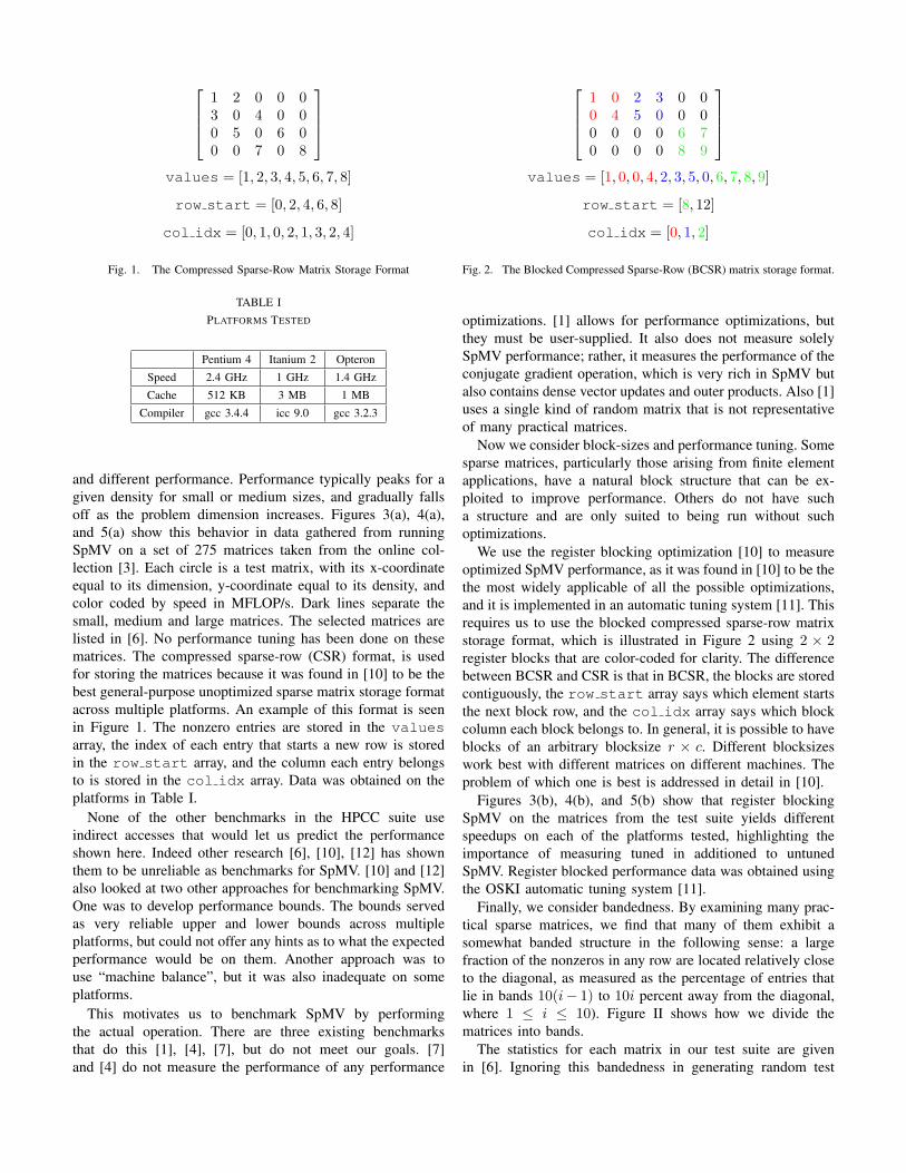
and different performance. Performance typically peaks for agiven density for small or medium sizes, and gradually fallsoff as the problem dimension increases. Figures 3(a), 4(a),and 5(a) show this behavior in data gathered from runningSpMV on a set of 275 matrices taken from the online col-lection [3]. Each circle is a test matrix, with its x-coordinateequal to its dimension, y-coordinate equal to its density, andcolor coded by speed in MFLOP/s. Dark lines separate thesmall, medium and large matrices. The selected matrices arelisted in [6]. No performance tuning has been done on thesematrices. The compressed sparse-row (CSR) format, is usedfor storing the matrices because it was found in [10] to be thebest general-purpose unoptimized sparse matrix storage formatacross multiple platforms. An example of this format is seenin Figure 1. The nonzero entries are stored in the valuesarray, the index of each entry that starts a new row is storedin the row start array, and the column each entry belongsto is stored in the col idx array. Data was obtained on theplatforms in Table I.

None of the other benchmarks in the HPCC suite useindirect accesses that would let us predict the performanceshown here. Indeed other research [6], [10], [12] has shownthem to be unreliable as benchmarks for SpMV. [10] and [12]also looked at two other approaches for benchmarking SpMV.One was to develop performance bounds. The bounds servedas very reliable upper and lower bounds across multipleplatforms, but could not offer any hints as to what the expectedperformance would be on them. Another approach was touse “machine balance”, but it was also inadequate on someplatforms.

This motivates us to benchmark SpMV by performingthe actual operation. There are three existing benchmarksthat do this [1], [4], [7], but do not meet our goals. [7]and [4] do not measure the performance of any performance

1 0 2 3 0 00 4 5 0 0 00 0 0 0 6 70 0 0 0 8 9

values = [1, 0, 0, 4, 2, 3, 5, 0, 6, 7, 8, 9]

row start = [8, 12]

col idx = [0, 1, 2]

Fig. 2. The Blocked Compressed Sparse-Row (BCSR) matrix storage format.

optimizations. [1] allows for performance optimizations, butthey must be user-supplied. It also does not measure solelySpMV performance; rather, it measures the performance of theconjugate gradient operation, which is very rich in SpMV butalso contains dense vector updates and outer products. Also [1]uses a single kind of random matrix that is not representativeof many practical matrices.

Now we consider block-sizes and performance tuning. Somesparse matrices, particularly those arising from finite elementapplications, have a natural block structure that can be ex-ploited to improve performance. Others do not have sucha structure and are only suited to being run without suchoptimizations.

We use the register blocking optimization [10] to measureoptimized SpMV performance, as it was found in [10] to be thethe most widely applicable of all the possible optimizations,and it is implemented in an automatic tuning system [11]. Thisrequires us to use the blocked compressed sparse-row matrixstorage format, which is illustrated in Figure 2 using 2 × 2register blocks that are color-coded for clarity. The differencebetween BCSR and CSR is that in BCSR, the blocks are storedcontiguously, the row start array says which element startsthe next block row, and the col idx array says which blockcolumn each block belongs to. In general, it is possible to haveblocks of an arbitrary blocksize r × c. Different blocksizeswork best with different matrices on different machines. Theproblem of which one is best is addressed in detail in [10].

Figures 3(b), 4(b), and 5(b) show that register blockingSpMV on the matrices from the test suite yields differentspeedups on each of the platforms tested, highlighting theimportance of measuring tuned in additioned to untunedSpMV. Register blocked performance data was obtained usingthe OSKI automatic tuning system [11].

Finally, we consider bandedness. By examining many prac-tical sparse matrices, we find that many of them exhibit asomewhat banded structure in the following sense: a largefraction of the nonzeros in any row are located relatively closeto the diagonal, as measured as the percentage of entries thatlie in bands 10(i− 1) to 10i percent away from the diagonal,where 1 ≤ i ≤ 10). Figure II shows how we divide thematrices into bands.

The statistics for each matrix in our test suite are givenin [6]. Ignoring this bandedness in generating random test

103 104 105

100

101

102

dimension

nnz/

row

Untuned Performance (MFLOP/s) of Real Matrices, P4

small

medium large

92

187

283

378

474

569

(a) Untuned SpMV performance

103 104 105

100

101

102

dimension

nnz/

row

Speedups Obtained by Tuning Real Matrices, P4

small

medium large

1.11

1.23

1.35

1.47

1.59

1.71

(b) Speedups obtained from tuning

Fig. 3. Small, Medium, Large behavior on the Pentium 4.

103 104 105

100

101

102

dimension

nnz/

row

Untuned Performance (MFLOP/s) of Real Matrices, Itanium 2

small

medium large

63

128

194

259

324

390

(a) Untuned SpMV performance

103 104 105

100

101

102

dimension

nnz/

row

Speedups Obtained by Tuning Real Matrices, Itanium 2

small

medium large

1.24

1.49

1.74

1.99

2.25

2.5

(b) Speedups obtained from tuning

Fig. 4. Small, Medium, Large behavior on the Itanium 2.

103 104 105

100

101

102

dimension

nnz/

row

Untuned Performance (MFLOP/s) of Real Matrices, Opteron

small

medium large

55

111

168

224

281

337

(a) Untuned SpMV performance

103 104 105

100

101

102

dimension

nnz/

row

Speedups Obtained by Tuning Real Matrices, Opteron

small

medium large

1.21

1.42

1.64

1.85

2.07

2.29

(b) Speedups obtained from tuning

Fig. 5. Small, Medium, Large behavior on the Opteron.

5@

@4

@@

@@

3

@@

@@

@@

2

@@

@@

@@

@@

1

@@

@@

@@

@@

2

@@

@@

@@

3

@@

@@

4@

@5

Fig. 6. Matrix divided up into bands. For simplicity of illustration, thismatrix is only divided up into 5 bands instead of 10.

matrices tends to underpredict performance, so we generateour matrices to match the statistics in [6].

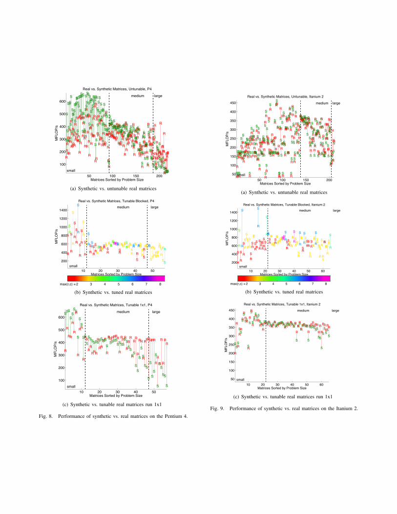
Randomly generated matrices matching all these criteria doa reasonably good job approximating the performance of thereal-life matrices they were created to model, as Figures 8–10show. In these plots, each real matrix is represented by an R,and is connected by a line to its synthetic counterpart, whichis represented by an S. The tuned plots are color-coded bylargest blocksize dimension.

One thing to note is that while a number of the matricesin our test suite are symmetric, the matrix generator we usedoes not generate symmetric matrices. To generate data fromwhich we could accurately gauge how well the syntheticmatrices performed, we ran the symmetric matrices from ourtest suite with symmetry disabled. We will return to the issueof symmetry in the last section.

III. THE BENCHMARK

We will now use what we have developed in the past twosections to construct a benchmark for SpMV. Our first task isto define the set of matrices from which we will take data.The test suite we used in the previous section has dimensionsranging from 512 to nearly a million, with densities rangingfrom 1 to almost 400 nonzero entries per row. We will considersquare matrices of similar dimensions, but only ones that arepowers of two ranging from 29 to 220. The number of nonzeroentries per row will range within [24, 34] = 29±5, since 29 isthe average number of nonzero entries per row in the suite. Thedistribution of nonzero entries will made to match statisticstaken from all of the matrices in the test suite, which are shownin Table II. The register blocksizes for optimized SpMV willcome from the set {1, 2, 3, 4, 6, 8} × {1, 2, 3, 4, 6, 8}. Thesewere the blocksizes most commonly found in work in [10] thatused a set of test matrices for which tuning showed benefits.

We take SpMV data from these matrices and report as out-put four MFLOP rates: unblocked maximum, unblocked me-dian, blocked maximum, and blocked median. The unblockednumbers are taken only from data gathered for matrices with1 × 1 blocks, and represent the case of the real-life matricesfor which tuning was attempted but found to be of no benefit.The tuned numbers are taken from the rest of the data, andrepresent the case of the real-life matrices for which therewas a benefit to tuning. Through these numbers, we seek to

TABLE IIDISTRIBUTION OF NONZERO ENTRIES IN MATRIX TEST SUITE

Distance From Diagonal Entries In This Range

0-10% 65.9%

10-20% 11.4%

20-30% 5.84%

30-40% 6.84%

40-50% 2.85%

50-60% 1.86%

60-70% 1.44%

70-80% 2.71%

80-90% 0.774%

90-100% 0.387%

TABLE IIIBENCHMARK RESULTS, FULL RUN

Unblocked Blocked

Max Median Max Median

Pentium 4 699 307 1961 530Itanium 2 443 343 2177 753Opteron 396 170 1178 273

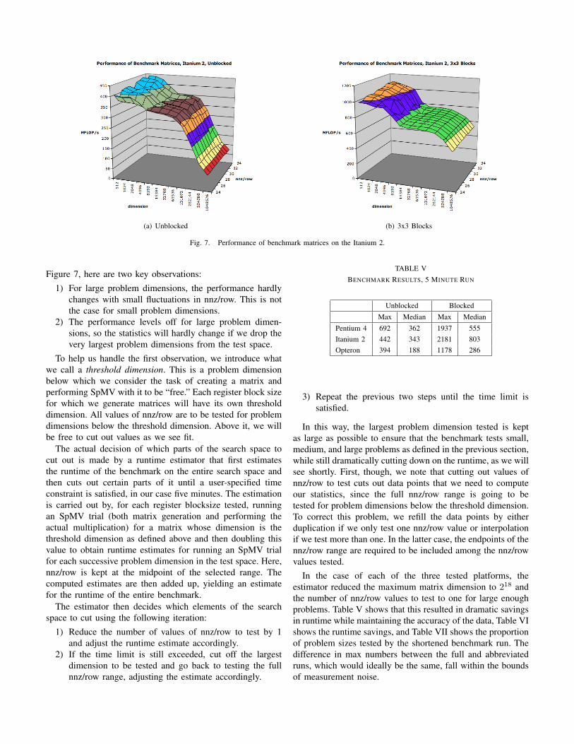
capture best-case and expected-case performance. Figure 7,which shows the performance of benchmark matrices withinour search space for two particular blocksizes on the Itanium2, illustrates why we select these numbers.

With the max numbers, we are looking to capture peakperformance, and with the median numbers, we are looking tocapture performance when it levels off. When forced to reportone number, as required by the HPCC suite’s rules, we willreport the blocked median. Table III shows the output for thethree platforms tested.

Figures 11–13 show that the numbers, especially the mediannumbers, give a good indicator of expected SpMV perfor-mance. Table IV reassures us that we tested small, medium,and large SpMV problems, and thus got a good set of data onwhich to base our benchmark numbers.

However, each of these runs took over 2 hours. If we wantto cut this down, we will need to prune the test space run bythe benchmark in such a way that we can capture the samedata while running far fewer SpMV trials. Looking back at

TABLE IVPROPORTION OF PROBLEM SIZES TESTED BY THE BENCHMARK, FULL

RUN

Pentium 4 Itanium 2 Opteron

Small 17% 33% 23%Medium 42% 50% 44%Large 42% 17% 33%

(a) Unblocked (b) 3x3 Blocks

Fig. 7. Performance of benchmark matrices on the Itanium 2.

Figure 7, here are two key observations:1) For large problem dimensions, the performance hardly

changes with small fluctuations in nnz/row. This is notthe case for small problem dimensions.

2) The performance levels off for large problem dimen-sions, so the statistics will hardly change if we drop thevery largest problem dimensions from the test space.

To help us handle the first observation, we introduce whatwe call a threshold dimension. This is a problem dimensionbelow which we consider the task of creating a matrix andperforming SpMV with it to be “free.” Each register block sizefor which we generate matrices will have its own thresholddimension. All values of nnz/row are to be tested for problemdimensions below the threshold dimension. Above it, we willbe free to cut out values as we see fit.

The actual decision of which parts of the search space tocut out is made by a runtime estimator that first estimatesthe runtime of the benchmark on the entire search space andthen cuts out certain parts of it until a user-specified timeconstraint is satisfied, in our case five minutes. The estimationis carried out by, for each register blocksize tested, runningan SpMV trial (both matrix generation and performing theactual multiplication) for a matrix whose dimension is thethreshold dimension as defined above and then doubling thisvalue to obtain runtime estimates for running an SpMV trialfor each successive problem dimension in the test space. Here,nnz/row is kept at the midpoint of the selected range. Thecomputed estimates are then added up, yielding an estimatefor the runtime of the entire benchmark.

The estimator then decides which elements of the searchspace to cut using the following iteration:

1) Reduce the number of values of nnz/row to test by 1and adjust the runtime estimate accordingly.

2) If the time limit is still exceeded, cut off the largestdimension to be tested and go back to testing the fullnnz/row range, adjusting the estimate accordingly.

TABLE VBENCHMARK RESULTS, 5 MINUTE RUN

Unblocked Blocked

Max Median Max Median

Pentium 4 692 362 1937 555Itanium 2 442 343 2181 803Opteron 394 188 1178 286

3) Repeat the previous two steps until the time limit issatisfied.

In this way, the largest problem dimension tested is keptas large as possible to ensure that the benchmark tests small,medium, and large problems as defined in the previous section,while still dramatically cutting down on the runtime, as we willsee shortly. First, though, we note that cutting out values ofnnz/row to test cuts out data points that we need to computeour statistics, since the full nnz/row range is going to betested for problem dimensions below the threshold dimension.To correct this problem, we refill the data points by eitherduplication if we only test one nnz/row value or interpolationif we test more than one. In the latter case, the endpoints of thennz/row range are required to be included among the nnz/rowvalues tested.

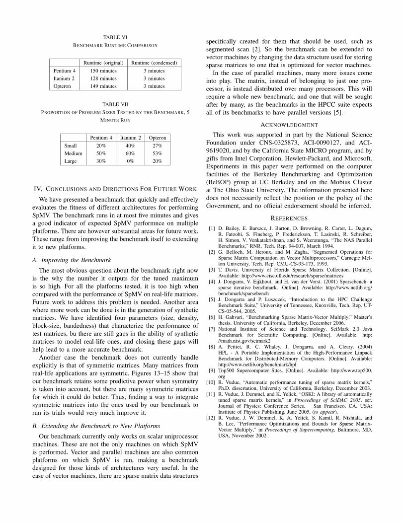
In the case of each of the three tested platforms, theestimator reduced the maximum matrix dimension to 218 andthe number of nnz/row values to test to one for large enoughproblems. Table V shows that this resulted in dramatic savingsin runtime while maintaining the accuracy of the data, Table VIshows the runtime savings, and Table VII shows the proportionof problem sizes tested by the shortened benchmark run. Thedifference in max numbers between the full and abbreviatedruns, which would ideally be the same, fall within the boundsof measurement noise.

TABLE VIBENCHMARK RUNTIME COMPARISON

Runtime (original) Runtime (condensed)

Pentium 4 150 minutes 3 minutesItanium 2 128 minutes 3 minutesOpteron 149 minutes 3 minutes

TABLE VIIPROPORTION OF PROBLEM SIZES TESTED BY THE BENCHMARK, 5

MINUTE RUN

Pentium 4 Itanium 2 Opteron

Small 20% 40% 27%Medium 50% 60% 53%Large 30% 0% 20%

IV. CONCLUSIONS AND DIRECTIONS FOR FUTURE WORK

We have presented a benchmark that quickly and effectivelyevaluates the fitness of different architectures for performingSpMV. The benchmark runs in at most five minutes and givesa good indicator of expected SpMV performnce on multipleplatforms. There are however substantial areas for future work.These range from improving the benchmark itself to extendingit to new platforms.

A. Improving the Benchmark

The most obvious question about the benchmark right nowis the why the number it outputs for the tuned maximumis so high. For all the platforms tested, it is too high whencompared with the performance of SpMV on real-life matrices.Future work to address this problem is needed. Another areawhere more work can be done is in the generation of syntheticmatrices. We have identified four parameters (size, density,block-size, bandedness) that characterize the performance oftest matrices, bu there are still gaps in the ability of syntheticmatrices to model real-life ones, and closing these gaps willhelp lead to a more accurate benchmark.

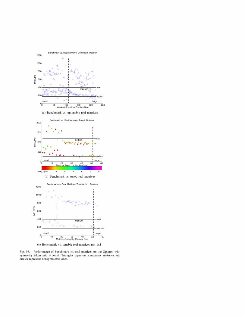
Another case the benchmark does not currently handleexplicitly is that of symmetric matrices. Many matrices fromreal-life applications are symmetric. Figures 13–15 show thatour benchmark retains some predictive power when symmetryis taken into account, but there are many symmetric matricesfor which it could do better. Thus, finding a way to integratesymmetric matrices into the ones used by our benchmark torun its trials would very much improve it.

B. Extending the Benchmark to New Platforms

Our benchmark currently only works on scalar uniprocessormachines. These are not the only machines on which SpMVis performed. Vector and parallel machines are also commonplatforms on which SpMV is run, making a benchmarkdesigned for those kinds of architectures very useful. In thecase of vector machines, there are sparse matrix data structures

specifically created for them that should be used, such assegmented scan [2]. So the benchmark can be extended tovector machines by changing the data structure used for storingsparse matrices to one that is optimized for vector machines.

In the case of parallel machines, many more issues comeinto play. The matrix, instead of belonging to just one pro-cessor, is instead distributed over many processors. This willrequire a whole new benchmark, and one that will be soughtafter by many, as the benchmarks in the HPCC suite expectsall of its benchmarks to have parallel versions [5].

ACKNOWLEDGMENT

This work was supported in part by the National ScienceFoundation under CNS-0325873, ACI-0090127, and ACI-9619020, and by the California State MICRO program, and bygifts from Intel Corporation, Hewlett-Packard, and Microsoft.Experiments in this paper were performed on the computerfacilities of the Berkeley Benchmarking and Optimization(BeBOP) group at UC Berkeley and on the Mobius Clusterat The Ohio State University. The information presented heredoes not necessarily reflect the position or the policy of theGovernment, and no official endorsement should be inferred.

REFERENCES

[1] D. Bailey, E. Barszcz, J. Barton, D. Browning, R. Carter, L. Dagum,R. Fatoohi, S. Fineberg, P. Frederickson, T. Lasinski, R. Schreiber,H. Simon, V. Venkatakrishnan, and S. Weeratunga, “The NAS ParallelBenchmarks,” RNR, Tech. Rep. 94-007, March 1994.

[2] G. Belloch, M. Heroux, and M. Zagha, “Segmented Operations forSparse Matrix Computation on Vector Multiprocessors,” Carnegie Mel-lon University, Tech. Rep. CMU-CS-93-173, 1993.

[3] T. Davis. University of Florida Sparse Matrix Collection. [Online].Available: http://www.cise.ufl.edu/research/sparse/matrices

[4] J. Dongarra, V. Eijkhout, and H. van der Vorst. (2001) Sparsebench: asparse iterative benchmark. [Online]. Available: http://www.netlib.org/benchmark/sparsebench

[5] J. Dongarra and P. Luszczek, “Introduction to the HPC ChallengeBenchmark Suite,” University of Tennessee, Knoxville, Tech. Rep. UT-CS-05-544, 2005.

[6] H. Gahvari, “Benchmarking Sparse Matrix-Vector Multiply,” Master’sthesis, University of California, Berkeley, December 2006.

[7] National Institute of Science and Technology. SciMark 2.0 JavaBenchmark for Scientific Computing. [Online]. Available: http://math.nist.gov/scimark2

[8] A. Petitet, R. C. Whaley, J. Dongarra, and A. Cleary. (2004)HPL - A Portable Implementation of the High-Performance LinpackBenchmark for Distributed-Memory Computers. [Online]. Available:http://www.netlib.org/benchmark/hpl

[9] Top500 Supercomputer Sites. [Online]. Available: http://www.top500.org

[10] R. Vuduc, “Automatic performance tuning of sparse matrix kernels,”Ph.D. dissertation, University of California, Berkeley, December 2003.

[11] R. Vuduc, J. Demmel, and K. Yelick, “OSKI: A library of automaticallytuned sparse matrix kernels,” in Proceedings of SciDAC 2005, ser.Journal of Physics: Conference Series. San Francisco, CA, USA:Institute of Physics Publishing, June 2005, (to appear).

[12] R. Vuduc, J. W. Demmel, K. A. Yelick, S. Kamil, R. Nishtala, andB. Lee, “Performance Optimizations and Bounds for Sparse Matrix-Vector Multiply,” in Proceedings of Supercomputing, Baltimore, MD,USA, November 2002.

50 100 150 200

100

200

300

400

500

600

R

S

R

S

R

S

R

SR

S

R

S

R

S

R

S

R

S

R

SR

S

R

SR

S

R

S

R

S

R

S

RS

R

S

R

S

RS

R

S

R

S

R

S

R

S

R

S

R

S

R

S

R

S

R

S

R

S

R

S

R

S

R

S

R

S

RS

RS

R

S

RS

R

S

R

S

R

SR

S

R

S

RS

R

S

R

S

R

SR

S

R

S

R

S

R

S

R

S

R

S

R

S

R

S

R

S

R

S

R

S

R

S

R

S

R

S

R

S

R

S

R

S

R

S

R

S

R

S

R

S

R

SR

S

R

SR

S

R

S

R

SR

S

R

S

R

S

R

S

R

S

R

S

R

S

R

S

R

S

R

SR

SRS

RSR

S

RS

R

S

RSRS

R

S

R

S

RS

R

S

R

S

R

S

R

S

R

S

R

S

R

S

R

SRS

R

SRS

R

S

R

SRS

RSRSRS

R

SRS

R

SRS

R

S

R

SRSR

S

R

SR

S

R

SRSRS

R

SRSRS

R

S

RS

R

S

R

SRS

R

SRSRSRSR

SR

S

RSRS

RSR

SRS

RS

R

S

RS

RS

RS

RSRS

RSR

SRS

RS

RS

RSR

SRSRSRSRS

RS

RS

RS

RS

RS

RS

RS

RSRSRS

R

S

RS

RS

RS

RS

RSR

SRS

RS

R

SR

S

RSRS

R

S

RS

RS

R

S

R

S

R

SRS

R

S

R

S

R

SRS

RSRSR

S

R

S

RS

R

SR

S

R

SRS

R

S

R

S

R

SR

S

R

SRS

R

SRS

R

S

R

S

R

S

R

S

R

S

Matrices Sorted by Problem Size

MFL

OP/

s

Real vs. Synthetic Matrices, Untunable, P4

small

medium large

(a) Synthetic vs. untunable real matrices

10 20 30 40 50

200

400

600

800

1000

1200

1400

Matrices Sorted by Problem Size

MFL

OP/

s

Real vs. Synthetic Matrices, Tunable Blocked, P4

R

SR

S

R

S

R

S

R

S

R

SR

S

R

SR

SR

S

R

SRSR

S

R

SRS

R

SR

S

R

SRSRSRSRSRS

RSRSRS

RSRSRSRS

RSRSRSRS

RSRSRS

RSRSRS

RS

RSRS

RSR

S

RSRSRSR

S

R

SR

SRSRSRS

RSR

S

R

Ssmall

medium large

max(r,c) = 2 3 4 5 6 7 8

(b) Synthetic vs. tuned real matrices

10 20 30 40 50

100

200

300

400

500

600

R

S

R

S

R

S

R

SR

S

R

SRS

R

S

R

S

RS

R

SRSRSR

S

R

S

R

S

R

S

R

SRSR

S

R

SRSRS

R

S

RSRSRSRSRSRS

R

SR

SRS

RS

R

SRS

R

S

RS

R

S

R

S

R

S

R

S

R

S

RS

R

S

R

S

R

S

R

S

R

S

R

S

R

SR

S

RS

R

SR

S

R

S

R

S

Matrices Sorted by Problem Size

MFL

OP/

s

Real vs. Synthetic Matrices, Tunable 1x1, P4

small

medium large

(c) Synthetic vs. tunable real matrices run 1x1

Fig. 8. Performance of synthetic vs. real matrices on the Pentium 4.

50 100 150 20050

100

150

200

250

300

350

400

450

RS

R

SRS

RS

RSRS

RS

RSRSRSR

S

RSRS

R

S

R

S

RSRSRSRS

RS

R

S

RS

RSRS

RSRS

RS

RS

RS

RS

RS

RSRS

RSRS

RS

RS

RS

RS

RSRSRS

RS

RS

RS

RS

RS

RS

RS

RS

RS

RSRSRS

RS

RS

R

S

RSRS

RS

RS

RS

RS

RS

RS

R

S

RSRSRS

RS

RSRS

RS

RSRS

RSR

S

RSRS

RSRSR

S

RS

R

SRS

RSRS

RS

RS

RS

R

S

RSRS

RS

R

S

R

S

R

S

RS

R

S

RS

RS

RS

RSRS

RS

RSRS

RSRS

RS

RSRS

RSRS

RSRS

RS

RS

RS

RS

RS

RS

RS

RS

RSRS

RS

RS

RSRS

RS

RS

RS

RSRS

RS

RS

RSRSRSRSRSRSRSRSRSRSRS

RSRSRS

RSR

S

RSRSRSRS

RS

RSRS

RS

RS

RS

RS

RS

RS

RS

RS

RS

RS

RSRSRS

RS

RS

RS

RS

RS

RS

RSRS

RS

RS

RS

RS

RS

RS

RS

R

SRSRS

RS

RSRS

R

S

R

S

RSR

S

R

SRSRS

R

S

RS

RS

RSRS

R

S

RS

R

S

RS

Matrices Sorted by Problem Size

MFL

OP/

s

Real vs. Synthetic Matrices, Untunable, Itanium 2

small

medium large

(a) Synthetic vs. untunable real matrices

10 20 30 40 50 60

200

400

600

800

1000

1200

1400

Matrices Sorted by Problem Size

MFL

OP/

s

Real vs. Synthetic Matrices, Tunable Blocked, Itanium 2

R

S

R

S

R

SR

S

R

SR

SRS

R

S

R

S

RS

RS

RS

RSRS

R

S

R

SRS

R

SR

S

R

S

R

S

RS

RSRS

RSRSRSRS

RSRSRSRSRSR

S

R

SRSRSRS

RSR

S

R

SRS

RS

R

SRS

RSR

S

RS

RSRS

RS

RSRS

RS

R

S

RS

RS

R

SRS

RS

RSRS

R

SRS

R

S

small

medium large

max(r,c) = 2 3 4 5 6 7 8

(b) Synthetic vs. tuned real matrices

10 20 30 40 50 6050

100

150

200

250

300

350

400

450

R

S

R

SRS

RSRS

RS

RSRSRS

RS

RS

RS

RSRSRS

RSRS

RSRSRSRSRSRS

RSRSRSRS

RSRSRSRSRSRSRS

RSRSRSRS

RSRSRSRS

R

S

RSRSRSRSRSRSRS

R

S

RSRSRSRS

RSRSRS

R

SR

S

R

S

RSRS

RSR

S

Matrices Sorted by Problem Size

MFL

OP/

s

Real vs. Synthetic Matrices, Tunable 1x1, Itanium 2

small

medium large

(c) Synthetic vs. tunable real matrices run 1x1

Fig. 9. Performance of synthetic vs. real matrices on the Itanium 2.

50 100 150 20050

100

150

200

250

300

350

400

450

R

S

R

S

R

S

R

SR

S

R

S

R

SR

S

R

S

R

S

R

S

R

S

R

S

R

S

R

S

R

S

R

S

R

S

R

S

R

S

R

S

R

S

R

S

R

S

R

S

R

S

R

SRS

R

S

RS

R

S

R

S

RS

R

S

R

S

R

S

RSR

S

R

S

R

S

R

S

R

SR

S

R

SR

S

R

S

R

SRSR

S

R

S

R

S

R

S

R

S

R

S

R

S

R

S

R

S

R

S

RS

R

SR

S

RS

R

S

RS

R

S

R

S

R

S

RSR

SRS

R

SRS

R

S

R

SR

S

RS

R

S

R

S

R

S

R

S

R

S

R

SR

SRSRS

R

SR

SR

S

R

S

R

S

R

S

RS

RS

R

S

R

S

R

SRS

R

S

RS

R

SRS

RS

R

S

R

S

R

SRSRSRS

RSRSRS

RSRS

RS

RS

RSRSRSRSRSRS

RS

RSRSRSRSRSRSRSRSRSRSRS

R

SRSRS

RSRSRSRSR

S

RSRSRSRS

RS

RS

R

SRSRSRSR

SRSRSRS

RS

RS

RSRSRS

R

SR

SRSRSR

S

R

SRS

RSRSR

SRS

R

SRSRSRS

RS

RSR

SR

S

R

S

R

S

R

SR

SRS

R

SR

S

R

S

R

S

R

SRS

R

SR

SRSRS

R

S

RSRSR

S

R

S

R

S

R

S

R

S

R

S

R

S

R

SRS

R

S

R

S

R

S

R

S

R

S

RS

RSRS

R

S

R

S

R

S

R

S

R

S

Matrices Sorted by Problem Size

MFL

OP/

s

Real vs. Synthetic Matrices, Untunable, Opteron

small

medium large

(a) Synthetic vs. untunable real matrices

10 20 30 40 50

200

400

600

800

1000

Matrices Sorted by Problem Size

MFL

OP/

s

Real vs. Synthetic Matrices, Tunable Blocked, Opteron

R

S

R

S

R

SR

S

RSRSRS

RS

RSR

S

R

S

R

S

RS

R

SR

S

RS

R

S

RSRSRSRSRSRS

RSRSRSRSRSRSRSR

SRSR

S

RSRSRSRSRSR

SRSRSRSRSRS

RSRSRSR

SRSRSR

S

RSRSRS

RSRS

small

medium large

max(r,c) = 2 3 4 5 6 7 8

(b) Synthetic vs. tuned real matrices

10 20 30 40 5050

100

150

200

250

300

350

400

450

R

S

RSR

S

RSRS

RSRS

RSRS

RS

RS

R

SRSRSRS

RS

RS

RSRSRSRSRSRSRSRS

RSRSRSRSRSRSRSR

S

RSRSRSR

S

RS

R

S

R

S

R

S

RSR

S

R

S

R

S

R

S

R

S

R

S

R

S

R

S

R

S

R

S

R

S

R

S

R

S

R

S

Matrices Sorted by Problem Size

MFL

OP/

s

Real vs. Synthetic Matrices, Tunable 1x1, Opteron

small

medium large

(c) Synthetic vs. tunable real matrices run 1x1

Fig. 10. Performance of synthetic vs. real matrices on the Opteron.

0 50 100 150 200 2500

100

200

300

400

500

600

700

median

max

small

medium

large

Matrices Sorted by Problem Size

MFL

OP/

s

Benchmark vs. Real Matrices, Untunable, P4

(a) Benchmark vs. untunable real matrices

0 10 20 30 40 50 600

500

1000

1500

2000

Matrices Sorted by Problem Size

MFL

OP/

s

Benchmark vs. Real Matrices, Tuned, P4

median

max

small

medium

large

max(r,c) = 2 3 4 5 6 7 8

(b) Benchmark vs. tuned real matrices

0 10 20 30 40 50 600

100

200

300

400

500

600

700

median

max

small

medium

large

Matrices Sorted by Problem Size

MFL

OP/

s

Benchmark vs. Real Matrices, Tunable 1x1, P4

(c) Benchmark vs. tunable real matrices run 1x1

Fig. 11. Performance of benchmark vs. real matrices on the Pentium 4.

0 50 100 150 200 2500

50

100

150

200

250

300

350

400

450

median

max

small

medium

large

Matrices Sorted by Problem Size

MFL

OP/

s

Benchmark vs. Real Matrices, Untunable, Itanium 2

(a) Benchmark vs. untunable real matrices

0 10 20 30 40 50 60 700

500

1000

1500

2000

2500

Matrices Sorted by Problem Size

MFL

OP/

s

Benchmark vs. Real Matrices, Tuned, Itanium 2

median

max

small

medium

large

max(r,c) = 2 3 4 5 6 7 8

(b) Benchmark vs. tuned real matrices

0 10 20 30 40 50 60 700

50

100

150

200

250

300

350

400

450

median

max

small

medium

large

Matrices Sorted by Problem Size

MFL

OP/

s

Benchmark vs. Real Matrices, Tunable 1x1, Itanium 2

(c) Benchmark vs. tunable real matrices run 1x1

Fig. 12. Performance of benchmark vs. real matrices on the Itanium 2.

0 50 100 150 200 2500

50

100

150

200

250

300

350

400

450

median

max

small

medium

large

Matrices Sorted by Problem Size

MFL

OP/

s

Benchmark vs. Real Matrices, Untunable, Opteron

(a) Benchmark vs. untunable real matrices

0 10 20 30 40 50 600

200

400

600

800

1000

1200

Matrices Sorted by Problem Size

MFL

OP/

s

Benchmark vs. Real Matrices, Tuned, Opteron

median

max

small

medium

large

max(r,c) = 2 3 4 5 6 7 8

(b) Benchmark vs. tuned real matrices

0 10 20 30 40 50 600

50

100

150

200

250

300

350

400

450

median

max

small

medium

large

Matrices Sorted by Problem Size

MFL

OP/

s

Benchmark vs. Real Matrices, Tunable 1x1, Opteron

(c) Benchmark vs. tunable real matrices run 1x1

Fig. 13. Performance of benchmark vs. real matrices on the Opteron.

0 50 100 150 200 2500

200

400

600

800

1000

1200

median

max

small

medium

large

Matrices Sorted by Problem Size

MFL

OP/

s

Benchmark vs. Real Matrices, Untunable, P4

(a) Benchmark vs. untunable real matrices

0 10 20 30 40 50 60 700

500

1000

1500

2000

Matrices Sorted by Problem Size

MFL

OP/

s

Benchmark vs. Real Matrices, Tuned, P4

median

max

small

medium

large

max(r,c) = 2 3 4 5 6 7 8

(b) Benchmark vs. tuned real matrices

0 10 20 30 40 50 60 700

200

400

600

800

1000

1200

median

max

small

medium

large

Matrices Sorted by Problem Size

MFL

OP/

s

Benchmark vs. Real Matrices, Tunable 1x1, P4

(c) Benchmark vs. tunable real matrices run 1x1

Fig. 14. Performance of benchmark vs. real matrices on the Pentium 4with symmetry taken into account. Triangles represent symmetric matricesand circles represent nonsymmetric ones.

0 20 40 60 80 100 120 140 1600

200

400

600

800

1000

1200

1400

medianmax

small

medium

large

Matrices Sorted by Problem Size

MFL

OP/

s

Benchmark vs. Real Matrices, Untunable, Itanium 2

(a) Benchmark vs. untunable real matrices

0 20 40 60 80 100 120 1400

500

1000

1500

2000

2500

3000

3500

Matrices Sorted by Problem Size

MFL

OP/

s

Benchmark vs. Real Matrices, Tuned, Itanium 2

median

max

small

medium

large

max(r,c) = 2 3 4 5 6 7 8

(b) Benchmark vs. tuned real matrices

0 20 40 60 80 100 120 1400

200

400

600

800

1000

1200

1400

medianmax

small

medium

large

Matrices Sorted by Problem Size

MFL

OP/

s

Benchmark vs. Real Matrices, Tunable 1x1, Itanium 2

(c) Benchmark vs. tunable real matrices run 1x1

Fig. 15. Performance of benchmark vs. real matrices on the Itanium 2 withsymmetry taken into account. Triangles represent symmetric matrices andcircles represent nonsymmetric ones.

0 50 100 150 200 2500

200

400

600

800

1000

1200

median

max

small

medium

large

Matrices Sorted by Problem Size

MFL

OP/

s

Benchmark vs. Real Matrices, Untunable, Opteron

(a) Benchmark vs. untunable real matrices

0 10 20 30 40 50 600

500

1000

1500

2000

Matrices Sorted by Problem Size

MFL

OP/

s

Benchmark vs. Real Matrices, Tuned, Opteron

median

max

small

medium

large

max(r,c) = 2 3 4 5 6 7 8

(b) Benchmark vs. tuned real matrices

0 10 20 30 40 50 600

200

400

600

800

1000

1200

median

max

small

medium

large

Matrices Sorted by Problem Size

MFL

OP/

s

Benchmark vs. Real Matrices, Tunable 1x1, Opteron

(c) Benchmark vs. tunable real matrices run 1x1

Fig. 16. Performance of benchmark vs. real matrices on the Opteron withsymmetry taken into account. Triangles represent symmetric matrices andcircles represent nonsymmetric ones.