BenchtopPIDController_WhPaper

7/18/2019 BenchtopPIDController_WhPaper

http://slidepdf.com/reader/full/benchtoppidcontrollerwhpaper 1/26

1

ithley Instruments, Inc.

775Aurora Road

eveland, Ohio 44139

40) 248-0400

x: (440) 248-6168

ww.keithley.com

Building a Benchtop PID ControllerRaymond Rogers

Keithley Instruments, Inc.

Proportional, integral, and derivative (PID) control is a feedback control

scheme widely used in engineering, science, and industry. The popularity of

PID is largely due to its ease of implementation and effectiveness. Motivation

for the use of PID stems from its cost-efficiency: a PID controller is never an

optimum controller but is good enough in most cases that the added cost and

complexity of an optimum controller is not worth the marginal increase in

performance. Furthermore, PID control does not require a deep understanding

of the underlying workings of a process; all that matters is that some measured

process variable can be strongly influenced by some controlled variable.

Although most PID controllers are dedicated instruments designed for

controlling specific processes, this white paper explores how to create a PID

controller with exceptional performance quickly and easily using standard

benchtop test equipment and minimal programming. Today, nearly all process

actuators (valves, agitators, heaters, motors, etc.) and process meters are

electronic, so the only two instruments required to build a PID controller are

a digital multimeter (to measure the process variable) and a power source (to

drive an actuator). In fact, many applications require only a voltmeter and a

unipolar power supply.

The acronym “PID” is derived from the controller’s constituent elements

and how they act on the difference between some desired value or set point

(SP) of a process variable and that variable’s current value. The process variable

(PV) of interest is often referred to as the measured (or manipulated) variable

(MV). The instantaneous difference between the SP and MV is known as the

error; the goal of the PID controller is to eliminate this error. In other words,

the controller works to ensure the process is operating in such a way that the

measured variable is always at the set point.



2

A PID controller is made up of three parts: the proportional part, which drives the

output in proportion to the instantaneous error; the integral part, which drives the output

in proportion to the accumulated error; and the derivative part, which drives the output

in proportion to the instantaneous rate of change of the error. Each part has a weighted

contribution to the total output signal of the controller. The process of establishing thoseweights in order to get the best response from the controller is known as tuning.

Not every controller requires all three PID elements: some are satisfactory with just

the proportional part and many others with just the proportional and integral parts. These

controllers are referred to as “P,” “PI,” “PD,” and “PID” in the context of PID control.

Each PID element is combined to create a controller with a unique and desired response.

The proportional part acts to eliminate the present error. As a result, a “P” controller is the

only feasible single-element PID controller. The integral part has a slow response but accounts

for process offsets that the proportional part cannot eliminate on its own. The derivative part

acts in response to the change in error. If the error is increasing, then the derivative output

adds to the total output; if the error is decreasing, then the derivative output subtracts from the

total output. The primary effect is that the derivative action responds strongly to quick changes

in the error but moderates the measured variable’s approach to the set point.

Tuning the PID controller involves giving each PID element the proper weight in order to

introduce desirable effects into the controller response while minimizing the drawbacks of

each element. The process to be controlled dictates what is desirable in the controller response.

For example, some processes may not accommodate overshoot well, which puts additional

limits on the rise time of the measured variable. On the other hand, another process may

accept some overshoot, allowing for a quick rise time of the measured variable.

PID Implementation

A DMM, a power supply, and a bit of programming are the only things required to build

a benchtop PID controller. Minimal programming experience is required because the PID

algorithm is relatively straightforward. A numerical realization of the PID controller will be

built upon its individual components. Figure 1 offers a graphic overview of PID control.



3

ΣSP(t) +

–

e(t)

uP(t)

u I (t)

u D

(t)

MV(t)

uP(t) = K

Pe(t)

u I (t) = K

I

e(t)d τ

∫

t

0

u D

(t) = K D

de(t)

dt

Σ+

+

+

u(t)

P

I

D

System

Figure 1. PID process diagram.

The PID controller takes the error as an input parameter and outputs a signal whose

magnitude is determined by the sum of the “P,” “I,” and “D” components of the PID

controller. Remember that the error is the difference between the desired value of some

process variable and that variable’s present value or the set point minus the measured value:

e(t) = SP(t) – MV (t)

The “P” contribution, u p(t), is determined by the following relation:

u p(t) = e(t)

By similar notation, the “I” and “D” contributions are defined thus:

t u I (t) = ∫ e(t )d t

0

de(t)uD(t) = _____

dt

The integral is run from the start of the controller to the present time. The total output,

u(t), is the weighted sum of each of the contributions:

u(t) = K PuP(t) + K I u I (t) + K Du D(t)

where K P, K I , and K D are the gain coefficients for each of the components as indicated by

their subscripts. The coefficients are user-supplied parameters and are determined through

tuning the controller for a particular use. The process of tuning is addressed in the section

titled “Tuning.”



4

e(t)

e(t)

S 1

S 0

t 1

t

MV

MV

Time

Setpoint

e(τ)dt

∫

t

0 de(t)dt

t 1

t

MV

Time

Figure 2. PID component contributions following a set point change from S 0 to S 1 at t 1.

The proportional component acts on the instantaneous error. The integral component acts

on the error accumulated since the beginning of the control loop. The derivative component

acts on the instantaneous rate of change of error. Figure 2 illustrates how these componentsare calculated.

It is important to note that the phrase “increasing error” could be misleading as to

whether the magnitude of e(t) is increasing or if e(t) has a positive slope. The derivative

component acts on the instantaneous slope of e(t) and can be negative even if the magnitude

is increasing, as is the case when the measured variable is deviating more and more above the

set point. The potential confusion arises from the fact that error has a sign associated with

it; a negative error indicates that the measured variable is above the set point. For the rest of

this white paper, “increasing error” means a positive slope of e(t), regardless of what the error

magnitude is doing.

The previous equations are realized numerically in this algorithm:

1. Determine the set point of the measured variable.

2. Make a measurement of the measured variable.



5

3. Measure the present time, call it tn, and calculate the time difference between the present

measurement and the previous measurement: ∆t n = t n – t n–1

4. Calculate the error: e(t n) = SP(t n) – MV(t n)

5. Determine each of the PID component outputs:

a. uP(t n) = e(t n)

b. u I (t n) = u I (t n–1) + 3(t n) * ∆t n

c.e(t n) – e(t n–1)u D(t n) =_____________

∆t n

6. Determine the total PID output from user-supplied gain coefficients:

a. u(t n) = K PuP(t n) + K I u I (t n) + K Du D(t n)

7. Begin again from step 1.

Keep two important details about this algorithm in mind. The first is that the loop takes a

finite amount of time to iterate through. If that time is controlled, then step 3 is unnecessary

because ∆t n is the same for every iteration. Furthermore, the multiplication and division by a

fixed ∆t n in steps 5b and 5c are not strictly necessary to carry out because they can be factored

out from each term and accounted for in the respective gain coefficients. The second detail is

that the loop is continued indefinitely until the controller is turned off.

The numerical integral and derivative presented in steps 5b and 5c are the simplest

approximations, that is, a Riemann Sum and a finite difference. Both have first-order error in

the time step. It is possible to make closer approximations for a given time step by using the

trapezoid rule (for example) for integration or a multi-point approximation for derivation.

The algorithm can be easily adapted to P, PI, or PD controllers by removing the

corresponding sub-step(s) in step 5 and the corresponding term(s) in step 6. Each of the three

components is computationally and functionally independent, so there are no extra steps

required when using less than full PID.

The output of the PID controller has been generalized and abstracted, but in practice

it will depend solely on the intended application. For instance, two PID controllers, each

from a separate process, may have the same output as determined from step 6. However, the

conversion from u(t n) to some meaningful physically controlled variable (such as voltage orcurrent) in order to drive a reactant flow rate or heating element is process dependent.

Some processes require a limit on the output so that the output of the PID does not drive

an actuator to failure or cause unnecessary stress. On the other hand, all actuators have

physical limits; a valve cannot open any wider than fully open. In these cases, it may be useful



6

to scale u(t n) as a ratio to fully open or fully actuated. It is generally easier to work with a PID

controller on both the coding and tuning sides if the output is appropriately scaled and limited

before tuning. Note that limits on the output must be hardcoded in some fashion.

As mentioned previously, PID controllers are easy to implement, in part because they can

be moved quickly from one process to another. The only changes needed will be to select an

appropriate output scale, the gain coefficients (via tuning), and maybe the output limits. This

modularity is a major reason PID controllers are so widely used.

The standard implementation would make use of a DMM to make voltage or current

measurements from an electronic sensor of some sort (a thermocouple, strain gauge, pressure

gauge, flow meter, etc.). The measurement would be fed into the PC running the PID

algorithm. The algorithm calculates the PID output and converts it to a source value for the

power supply. The power supply sources into some sort of electronic actuator (heating element,

motor, pump, valve, etc.), which drives the measured variable toward the process set point.

LabVIEW Implementation

Implementing a PID controller via software is the simple matter of realizing the previous

algorithm numerically. National Instruments’ LabVIEW programming environment is

used here to demonstrate a PID controller implementation for two reasons. The first is that

LabVIEW is widely used in industry and research and second is that the flowchart-like

representation of the code serves well to show how everything fits together. An example

PID controller written in LabVIEW is availalbe for download at http://www.keithley.com/

data?asset=57762.

Figures 3, 4, and 5 show the block diagrams of the “P,” “I,” and “D” components of a PID

controller. Figure 6 shows how all of them fit into a single subVI (a.k.a. a subroutine).

Figure 3. LabVIEW implementation of “P.”

http://www.keithley.com/data?asset=57762






7

Figure 4. LabVIEW implementation of “I.”

Figure 5. LabVIEW implementation of “D.”



8

Figure 6. LabVIEW implementation of “PID.”

As Figure 3 indicates, the proportional component is the simplest; it takes the error and

gain coefficient as inputs and multiplies them together. The integral component takes the error,

gain coefficient, and time since start as inputs. The time step is accomplished by subtracting

the previous timing from the current timing via a feedback node. The integral is kept as a

running tally (Riemann Sum) of the error, which is then multiplied by the gain coefficient.

The derivative component keeps track of the time in the same way as the integral but also

keeps track of the previous error. The change in error is divided by the change in time toapproximate the derivative via a finite difference. The smaller subVIs can be used when only a

“P” or “PI,” for example, is needed. Otherwise, the total PID subVI is available when all three

components are needed.

The PID controller takes in six inputs: the present value (measurement), the set point, the

time since the start of the controller, and all three of the gain coefficients. The controller has

four outputs: the total output and the output for each of the three components. Each of the six

inputs must be supplied, but any of the outputs can be used.

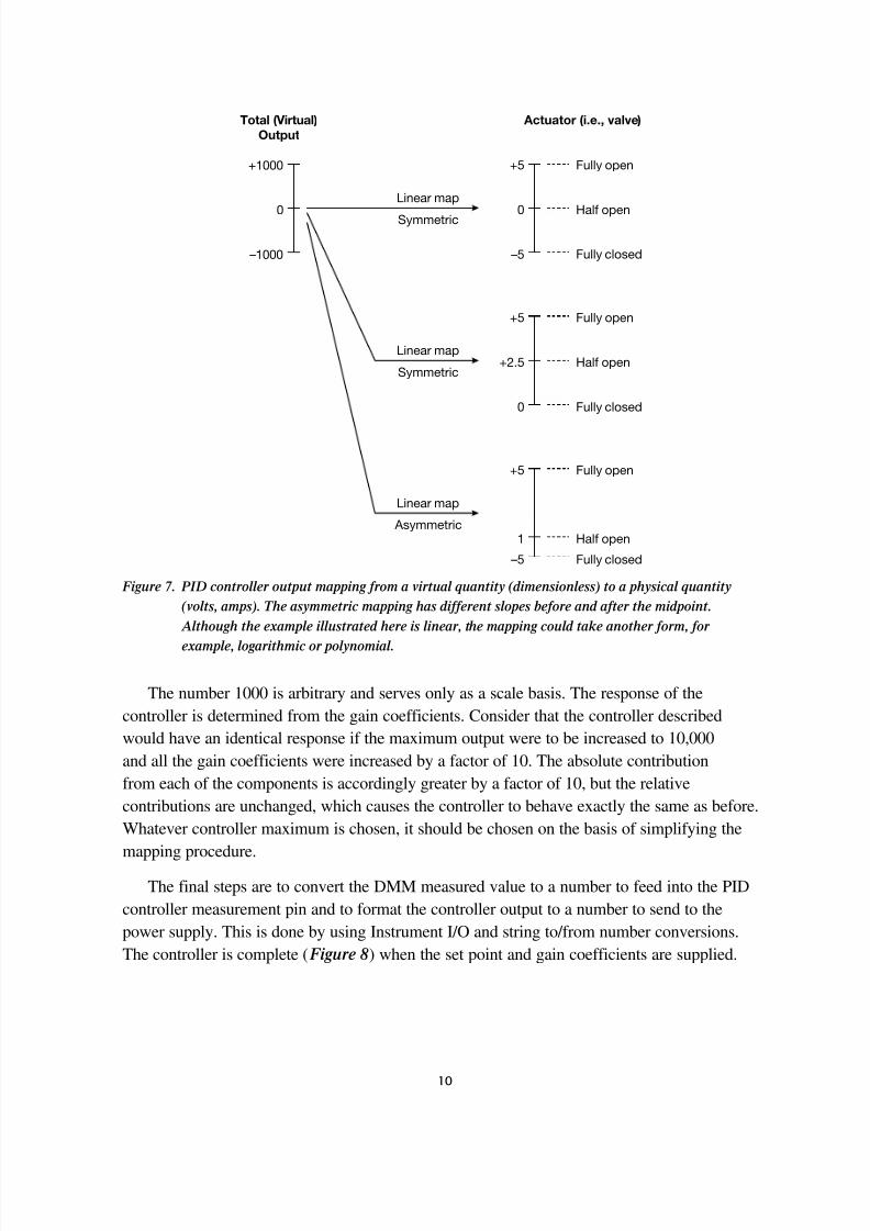
The output of the PID controller is simply a number. That number needs to be convertedinto something that’s meaningful to the physical system being controlled, such as the source

value for the power supply. Furthermore, it is possible that the user may want to limit the

source value further to a certain range. Thus, the output of the controller must be mapped to

the range to be used.



9

For example, if the actuator to be controlled is determined to safely accept between 0V and

5V then the number out of the PID controller needs to be mapped to fall within that range.

The midpoint of the range also needs to be determined and the controller output mapped so

that an output of zero gets mapped to the midpoint.

The midpoint is best defined as the ideal point at which lower source values decrease

the measured variable and higher source values increase the measured variable. This poses

a problem of definition because the midpoint can very well end up dynamic and dependent

on the current state of the system to be controlled, particularly if there are system losses in

proportion to the measured variable. One manifestation of this dynamic behavior is what’s

known as droop (see the section titled “Droop and Windup” for details). Ultimately, the

midpoint is an estimate that is close to the ideal point for the majority of system states,

particularly in the region of control interest. This is not a big problem because the PID

controller is self-regulating and any significant deviation is corrected primarily through the

integral term.

The simplest way to map the controller output is to choose an arbitrary maximum, such

as 1000. All that is required is to map the output of the controller linearly so that an output of

–1000 gives 0V and 1000 gives 5V. The midpoint is determined to be 2.5V and an output of 0

maps to 2.5V. Figure 7 illustrates various mapping procedures.



10

Total (Virtual)

Output

Actuator (i.e., valve)

+5

0

–5

Fully open

Linear map

Symmetric Half open

Fully closed

+1000

0

–1000

+5

+2.5

0

Fully open

Linear map

SymmetricHalf open

Fully closed

+5

1

–5

Fully open

Linear map

AsymmetricHalf open

Fully closed

Figure 7. PID controller output mapping from a virtual quantity (dimensionless) to a physical quantity

(volts, amps). The asymmetric mapping has different slopes before and after the midpoint.

Although the example illustrated here is linear, the mapping could take another form, for

example, logarithmic or polynomial.

The number 1000 is arbitrary and serves only as a scale basis. The response of the

controller is determined from the gain coefficients. Consider that the controller described

would have an identical response if the maximum output were to be increased to 10,000

and all the gain coefficients were increased by a factor of 10. The absolute contribution

from each of the components is accordingly greater by a factor of 10, but the relative

contributions are unchanged, which causes the controller to behave exactly the same as before.

Whatever controller maximum is chosen, it should be chosen on the basis of simplifying the

mapping procedure.

The final steps are to convert the DMM measured value to a number to feed into the PID

controller measurement pin and to format the controller output to a number to send to the

power supply. This is done by using Instrument I/O and string to/from number conversions.

The controller is complete ( Figure 8) when the set point and gain coefficients are supplied.



11

Figure 8. Full PID Controller employing a Keithley Model 2000 DMM to monitor the measured variable

and a Keithley Model 2200 Power Supply to power the actuator. The subVI shown in Figure 6

is the KI-PID block seen in the center here. An example PID controller written in LabVIEW is

available for download at http://www.keithley.com/data?asset=57762.

Tuning

Although implementing the PID controller is relatively straightforward, tuning the controller

is a more open-ended aspect of PID control. Tuning is not a simple process because it requires

understanding how each of the PID components affects the response. A poorly designed PID

controller will display one or more of the following performance problems: oscillation, poor

damping, overshoot, slow rise/fall times, kick, droop, and excessive windup. This section

describes each of these problems and their primary causes.

OscillationOscillation is one of the more complicated performance issues and can be the result of several

factors. The most common cause is too large a proportional gain ( Figure 9) for the loop

iteration rate (frequency) of the PID controller. A second cause is a mostly integral controller;

the proportional acts as a dampener in this case. Thirdly, and easily overlooked, is that the

physical system being controlled could be oscillatory in nature and the PID controlling

this system may have to accept some oscillation. This does not necessarily indicate a poor

PID controller.





12

0

0.5

1

1.5

2

2.5

3

0 0.1 0.2 0.3 0.4 0.5 0.6 0.7 0.8 0.9 1

M e a s u r e d V a r i a b l e M a g n i t u d e ( a r b )

Time (arb)

Kp = 1

Kp = 1.1

Kp = 1.8

Kp = 5

Set Point

Figure 9. Measured variable response to proportional gain coefficient.

An integral-heavy PID controller will also oscillate ( Figure 10) because the error

accumulated while the measured variable is below the set point takes time to correct while the

measured variable is over the set point. The integral component then starts to accumulate error

in the opposite direction, which will not be corrected until the measured variable crosses the

set point again. The proportional component will act as a dampener in this situation.



13

0

0.5

1

1.5

2

2.5

3

3.5

0 0.1 0.2 0.3 0.4 0.5 0.6 0.7 0.8 0.9 1


Time (arb)

Kp = 1, Ki =3

Kp = 1, Ki = 30

Set Point

Figure 10. Oscillation due to high integration gain coefficient.

The frequency of the controller is the rate at which the control loop operates and the power

supply output is updated once per cycle. This single-update behavior can be problematic if

the proportional gain is too high. A small error produces a large output, which causes a large

change in the measured variable, even in one cycle. If that change takes the measured variable

past the set point, then the output reverses polarity for the next cycle. If the measured variable

keeps jumping across the set point from cycle to cycle, then the controller is oscillating. If

the gain is high enough and causes the measured variable to jump across with increasing

error magnitude, then the controller is deemed unstable. The quickest fix is to lessen the

proportional gain. However, increasing the controller frequency, if possible, will help as well.

This is an inherent limitation of a digital controller; there will always be some degree

of oscillation. In addition to the loop frequency issue already described, the output of the

power supply can only be resolved to some finite value and nothing smaller. The problem

then becomes a question of how much can the oscillation be reduced. A perfectly continuous

controller would not have this problem because the output is continually updating along with

the changing error. However, oscillation from frequency limitations still occurs in analog

PID control. Such controllers are analog circuits and they still have an effective operation

frequency resulting from reactive components that cause a time lag between output and input.



14

Oscillation due to a high integral gain can be reduced either by reducing the integral gain

(the obvious solution) or by increasing the proportional gain (not immediately obvious). The

proportional action will dampen the oscillations caused by the integral action. This example

showcases the difficulty of tuning and the user must decide which characteristics of controller

responses are required, desired, and unacceptable. Each characteristic has a tradeoff associatedwith it and the priority of the controller characteristics should be established before attempting

to tune the system.

Droop and Windup

Most physical systems have some sort of parasitic mechanism that causes a loss or reduction of

the measured variable. For example, a heater/cooler system must take heat loss/gain through

system boundaries into consideration. The effort of a proportional-only control system will

always reduce to the point where the controller output is just enough to bring the measured

variable to the set point minus system losses. This point is where the controller output is not

enough to change the error but just enough to keep it constant – a steady-state error, in other

words. This phenomenon, known as droop ( Figure 11), prevents the measured variable from

reaching the set point. Despite the term “droop,” the offset can be either below or above the set

point as it depends on the state of the physical system being controlled.



15

0

0.5

1

1.5

2

2.5

0 0.1 0.2 0.3 0.4 0.5 0.6 0.7 0.8 0.9 1


Time (arb)

Kp = 1

Set Point

Figure 11. PID “droop.”

One’s first instinct might be to increase the proportional gain in an attempt to lessen the

droop amount. But that is all increasing the proportional gain will do; a proportional-only

controller will always encounter droop because there is nothing to account for system losses.For some systems, a small droop may be acceptable and a proportional-only controller remains

useful. For other systems, droop is undesirable and increasing the proportional gain may

introduce more problems, such as oscillation and set point overshoot.

The heater/cooler mentioned previously represents a generic temperature control system,

complete with boundaries and temperature differences across them. Accurately controlling

the system temperature and accounting for droop may require a complicated algorithm

relating temperature gradients and time constants. Alternatively, the proportional-only

controller may expand to a PI controller and allow the integral component to account for

droop ( Figure 12). The output of the controller will continually increase (or decrease) whilethe measured variable is less than (or greater than) the set point. The integral component

builds up a “buffer” and establishes it as an offset of the controller output that compensates for

system losses.



16

0

0.5

1

1.5

2

2.5

0 0.1 0.2 0.3 0.4 0.5 0.6 0.7 0.8 0.9 1


Time (arb)

Kp = 1, Ki = 1.5

Set Point

"Droop" Line

Figure 12. Integration correction to droop.

The time required for the integral component to build this buffer from the start of the

controller is known as windup. There may also be a significant windup period following a

large set point change because the integral offset required at one set point is different than theoffset required at another set point. Some control systems start a control loop with a non-zero

addition to the integral term in an attempt to reduce the initial windup.

A large set point change can also induce a long windup. This effect can be reduced

by stopping the integral mechanism from accumulating while the output is already at an

extremum. This is because the integral term is not affecting the output but is still accumulating

error, which will have to be cancelled out later.

Rise Time and Overshoot

The rise (or fall) time of the measured variable is the time it takes for the measured variable

to reach the set point following a change. A fast rise time is desirable for obvious reasons, but

too fast a rise time will cause an overshoot of the measured variable across the set point. The

overshoot may then result in damped oscillation as the measured variable settles out to the set

point. For some applications, some overshoot is an acceptable tradeoff for a short rise time.



17

For others, no overshoot can be tolerated and carefully selecting the PID component gains can

produce the fastest rise time with no overshoot.

Rise time is principally affected through the proportional and derivative gains. The

derivative action responds strongly to an abrupt change but slows the approach to the set point.

The integral component doesn’t affect rise time appreciably because of its error accumulation

nature but can cause overshoot. Furthermore, as described previously, a large integral gain will

cause oscillation.

The rise time is typically defined as the time for the variable of interest to rise from 10%

of the final value to 90% of the final value. This is the definition used here.

Disturbance Robustness

A disturbance occurs when anomalies in any of the process variables cause an abrupt or

unusual change in the measured variable, such as a pipe burst in a feedstock that causes a

dramatic drop in vessel pressure (the measured variable). A malfunction of a pre-heating

phase in a process, which causes the system temperature to droop much lower than during

normal operation, is another typical example. Disturbance robustness is then a property of a

PID controller to handle these changes effectively.

Disturbances may or may not be accounted for in a process scheme. This means that a

controller attempting to control a process without a feedback loop would certainly fail to

account for a disturbance simply because it is difficult to consider every possible source of a

disturbance. One of the biggest advantages of a PID controller is that it can be tuned to reject

disturbances, even if they originate with something seemingly unrelated (or unconsidered) to

the process at hand.

An abrupt change in the measured variable can be viewed as functionally equivalent to a

step change of the set point ( Figure 13). Therefore, the tuning performed to ensure the best

response to a step change of the set point will do much the same for disturbance rejection.

This is the case unless the disturbance affects the PID controller’s ability to control the

measured variable, either because the actuation becomes compromised or the disturbance

brings the measured variable near or outside of the actuation boundaries. The burst pipe

mentioned previously would be an example of compromised actuation; controlling the pressure

inside a breached pipe will surely overtax the pump.



18

-500

-400

-300

-200

-100

0

100

200

300

400

500

0 0.1 0.2 0.3 0.4 0.5 0.6 0.7 0.8 0.9 1

C o n t r o l l e r O u t p u t A c t o n ( a r b )

Time (arb)

Controller Response to Disturbances and Step Changes

Figure 13. Each peak is either a step change or a sudden disturbance. The two are indistinguishable.

Kick, Noise, and the Derivative Action

Figure 13 displays the usual controller response to a step change or disturbance. The issue topoint out is that the response is an abrupt spike. This is known as kick and can be undesirable

for several reasons: this sort of response may be stressing the power supply or actuator

unnecessarily or the controller output could be telling a power supply to force a current into an

inductive load, such as a motor. If kick is undesirable, consider one of the following options:

• Hard code a limit to how much the output can change from iteration to iteration. This

may not impact the controller performance appreciably if kick is determined to occur

on certain extreme conditions. Otherwise, the limit will affect the rise time of the

measured variable.

• Consider that the derivative action has the potential to cause a very high kick due

to division by a very small time step. The solution may be to remove the derivative

component completely.

A related problem, particularly with the derivative action, is that of noise. The small rapid

changes in the measured variable can be magnified to large controller responses solely from



19

the derivative action. The problem is that the derivative term needs to be large enough to have

an appreciable effect on the controller output, but the larger the derivative term is, the more

adversely it amplifies noise. The easiest solution is to include a dead-band of error change to

which the derivative component does not respond, that is, has a set output of zero.

Frequency

The control loop frequency is understood to be the rate at which a control loop operates.

The inverse is the period (T) and corresponds to the time in between iterations of the loop.

Frequency is an important parameter because it determines what kind of systems the PID loop

can adequately control. Consider that every physical system has a time constant associated

with the measured variable. In other words, how fast does the measured variable change with

an associated change in the actuator?

This is important because, if the period of the PID loop is much greater than the time

constant of the measured variable, then the measured variable will not be able to be broughtto the set point, if at all, on an order of time faster than T. For instance, if the output is

determined to increase the measured variable for the next T seconds, then the measured

variable will be increasing by some rate associated with the system’s time constant. The

measured variable might very well overshoot the set point in that time, possibly drastically.

The output will not be updated until the next iteration, which will then respond to decrease the

measured variable for the following T seconds. The end result is an oscillation and the only

way to reduce, but not eliminate, this oscillation is to have the controller respond weakly (low

gain coefficients) to the error. In effect, this increases the time constant of the physical system

to the period of the control loop and the potential for fast control is wasted.

If the period is much smaller than the time constant of the physical system, then the

controller is over-designed for the application. This doesn’t have a drawback in controlling the

system, per se, but the controller itself may be more expensive or harder to build, maintain,

and run due to specialized parts, faster clocks, etc.

The period of a control loop can be determined from its implementation. To first

approximation, the period is equal to the slowest running part of the entire system, be it the

meter, power supply, actuator, etc. If the power supply takes 100ms to respond to commands

from a host PC running a software PID, then the period is 100ms, assuming the meter and

PID loop itself can respond quicker. The software loop can certainly run faster, but the powersupply won’t be changing any quicker than once every 100ms.

The best way to tune a PID controller is first to decide which kind of control response is

desired. Is a fast rise time needed? Can there be any oscillation? Is the process to be controlled

too fast for my equipment? Start by using only the proportional component and then add in the



20

integral and derivative as the proportional-only inadequacies become apparent. A well-tuned

PID controller is an effective and simple solution to many process control needs.

Temperature Control Example

This example describes the implementation of a simple PID scheme that employs aPeltier device, a J-type thermocouple, a Keithley Model 2000 DMM, a Keithley Model

2200-20-5 power supply unit, and the PID algorithm as run on a National Instruments’

LabVIEW application. It allows controlling temperature to within ±0.05°C under most

operating conditions with just a J-type thermocouple and no shielding of the signal line. The

implementation is a temperature controller that consists of the Peltier device sandwiched

between a bottom aluminum plate and an insulator. The bottom plate is contained within

an ice-water bath and the PID loop controls the temperature of a small aluminum plate

underneath the insulator ( Figure 14). This example demonstrates the effectiveness of a PID

loop, even when run from a PC.

The DMM is used to collect voltage measurements from the thermocouple. These

readings are internally converted to temperature measurements, which are fed as the

measured variable into the PID loop running on the LabVIEW application. The loop then

compares these measurements against the user-supplied set point and an appropriate output

is determined via the PID algorithm. The output is converted to a current to be sourced by

the power supply into the Peltier device. The current ranges between 0A and 5A.

Aluminum Heat Sink

+ TEC –

HI

LO

HI

LO

Model 2000

DMM

Model 2200-20-5

Power Supply

Figure 14. The heat sink is kept at a constant temperature by placing it in an ice bath.

Some details about the PID system require clarification. For example, the Model

2200-20-5 is a unipolar power supply, which is not necessarily a problem, but it does mean

that the top aluminum plate will have to cool passively. The concern is the rate of passive

cooling vs. that of active heating. The difference can be significant unless the region of

control is chosen such that the control midpoint is the center of the power supply’s output



21

range, namely 2.5A. This occurs at about 80°C for this system. At this temperature, any

current less than 2.5A fed into the Peltier will cause the top plate to cool down. In other

words, active heating and passive cooling are symmetric about 2.5A at this temperature.

The second detail is that the PID loop is operating at 20Hz or 50ms per cycle. The risetime associated with this system is several seconds, which is much longer than the PID

loop period. The loop period could be increased to about one second before any significant

performance degradation becomes apparent.

The last detail is that the PID output is linearly mapped so that an output of –1000

correlates to 0A and an output of 1000 correlates to 5A. This gives the 0A to 5A range with

a 2.5A midpoint described previously. The ±1000 output of the controller dictates the order

of magnitude of the gains. Again, be aware that these numbers are completely arbitrary; the

output could have been mapped to ±100 instead and the gains seen in the following figures

would be ten times less for identical responses.

A dead-band for the derivative action and a controlled accumulator for the integral

action were implemented as discussed in the “Tuning” section as a way to reduce the

derivative response to noise and the integral windup respectively. The dead-band has a user-

settable threshold and the integral does not accumulate error if the controller is already

operating at maximum output.



22

74

76

78

80

82

84

86

0 5 10 15 20 25 30 35

T e m p e r a t u r e ( C )

Time (s)

Kp 200

Kp 400

Kp 600

Kp 1200

Set Point

Figure 15. Temperature controller proportional-only droop.

The PID controller is run at several different gain coefficients in order to demonstrate

tuning and the problems involved in it as discussed in the “Tuning” section. Figure 15

illustrates the primary problems associated with a P-only controller: droop and oscillation.

Increasing the proportional gain only reduces the droop; it will never eliminate it.

Furthermore, too high a proportional gain will introduce oscillation into the response. The

rise time is approximately nine seconds.



23

74

76

78

80

82

84

86

0 20 40 60 80 100 120


Time (s)

Kp 100, Ki 5

Kp 100

Set Point

Figure 16. Temperature controller integral correction to droop.

Figure 16 shows how adding even a small integral gain will correct the droop of a

proportional-only controller. The speed of this correction depends strongly on the integral

gain. The rise time of the PI trace is about nine seconds, but the settling time from the

overshoot extends for more than a minute.



24

74

76

78

80

82

84

86

0 10 20 30 40 50 60


Time (s)

Kp 400

Kp 400 Ki 50

Kp 400 Ki 200

Set Point

Figure 17. Temperature controller integral heavy oscillation.

Figure 17 demonstrates that a moderate integral gain will quickly correct droop,

but adding too much will introduce oscillations. One of the best responses seen for this

controller was the black trace (Kp 400, Ki 50). The rise time of this trace is approximately

nine seconds and the measured variable settles to 1% of the set point in approximately six

seconds after the rise time. The response settles to within ±0.05°C of the set point afterabout eleven more seconds.



25

74

76

78

80

82

84

86

0 5 10 15 20 25

Kp 600

Kp 600 kd 100

Kp 600 Kd 200

Kp 600 Kd 600

Set Point

Figure 18. Temperature controller derivative damping.

Figure 18 shows how a derivative gain slows the approach to the set point. A high

derivative gain will introduce artifacts into the response, resulting from the derivative action

on noise. These artifacts can easily lead to system instability because the change resulting

from a derivative action against a noise spike will cause the derivative action in the next

loop iteration to be stronger and so on. The red trace (Kp 600, Kd 600) shows that theartifacts will emerge randomly and can be sustained for upwards of a second. The controller

would be significantly less stable without the dead-band mentioned previously.



Specifications are subject to change without notice. All Keithley trademarks and trade names are the property of Keithley Instruments, Inc.

All other trademarks and trade names are the property of their respective companies.

KEITHLEY INSTRUMENTS, INC. ■ 28775AURORA RD. ■ CLEVELAND, OH 44139-1891 ■ 440-248-0400 ■ Fax: 440-248-6168 ■ 1-888-KEITHLEY ■ www.keithley.co

A Greater Measure of Confiden

BENELUX+31-40-267-5506www.keithley.nl

BRAZIL

55-11-4058-0229www.keithley.com

CHINA

86-10-8447-5556www.keithley.com.cn

FRANCE+33-01-69-86-83-60www.keithley.fr

GERMANY

+49-89-84-93-07-40www.keithley.de

INDIA

080-30792600www.keithley.in

ITALY+39-049-762-3950www.keithley.it

JAPAN

81-120-441-046www.keithley.jp

KOREA

82-2-6917-5000www.keithley.co.kr

MALAYSIA 60-4-643-9679 www.keithley.com

MEXICO

52-55-5424-7907 www.keithley.com

RUSSIA

+7-495-664-7564 www.keithley.ru

SINGAPORE01-800-8255-2835www.keithley.com.sg

TAIWAN

886-3-572-9077www.keithley.com.tw

UNITED KINGDOM

+44-1344-39-2450www.keithley.co.uk

For further information on how to purchase or to locate a sales partner please visit www keithley com/company/buy

http://www.keithley.com/company/buy

http://www.keithley.com/company/buy

Date post:	01-Mar-2016
Category:	Documents
Upload:	firosekhan
View:	5 times
Download:	0 times

BenchtopPIDController_WhPaper

Documents