TUTORIAL BENDERS DECOMPOSITION IN RESTRUCTURED POWER SYSTEMS Mohammad Shahidehpour and Yong Fu Electric Power and Power Electronics Center Illinois Institute of Technology Chicago, Il 60616 {ms, fuyong}@iit.edu 1. Introduction It is apparent that the power system restructuring provides a major forum for the application of decomposition techniques to coordinate the optimization of various objectives among self-interested entities. These entities include power generators (GENCO), transmission providers (TRANSCO), and distribution companies (DISCO). Consider a decomposition example when individual GENCOs optimize their annual generating unit maintenance schedule based on their local constraints such as available fuel, emission, crew, and seasonal load profile. The GENCO’s optimization intends to maximize the GENCO’s payoff in a competitive environment. Individual GENCOs submit their maintenance schedule to the ISO which examines the proposed schedule to minimize the loss of load expectation while maintaining the transmission security based on the available transfer capacity, and forced and scheduled outages of power system components. The ISO could return then proposed schedule to designated GENCOs in case the operating constraints would be violated. The ISO’s rejection of the proposed schedule could include a suggestion (Benders cut) for revising the proposed maintenance schedule that would satisfy GENCOs’ and the ISO’s constraints. Earlier in the 1960-1970, many of the decomposition techniques were motivated by inability to solve large-scale centralized problems with the available computing power of that time. The dramatic improvement in computing technology since then allowed power engineers to solve very large problems easily. Consequently, interest in decomposition techniques dropped dramatically. However, now there is an increasingly important class of optimization problems in restructured power systems for which decomposition techniques are becoming most relevant. In principle, one may consider the optimization of a system of independent entities by constructing a large-scale mathematical program and solving it centrally (e.g., through the ISO) using currently available computing power and solution techniques. In practice, however, this is often impossible. In order to solve a problem centrally, one needs the complete information on local objective functions and constraints. As these entities are separated geographically and functionally, this information may be unattainable or prohibitively expensive to retrieve. More importantly, independent entities may be unwilling to share or report on their propriety information as it is not incentive compatible to do so; i.e., these entities may have an incentive to misrepresent their true preferences. In order to optimize certain objectives in restructured power systems, one must turn to the coordination aspects of decomposition. Specifically, with limited information one must coordinate entities to reach an optimal solution. The goal will be to coordinate the entities by optimizing a certain objective (such as finding equilibrium resource price) while satisfying local and system constraints. One of the commonly used decomposition techniques in power systems is Benders decomposition. J. F. Benders introduced the Benders decomposition algorithm for solving large-scale mixed-integer programming (MIP) problems. Benders decomposition has been successfully applied to take advantage of underlying problem structures for various optimization problems, such as restructured power systems 1
Transcript
TUTORIAL
BENDERS DECOMPOSITION IN RESTRUCTURED POWER SYSTEMS
Mohammad Shahidehpour and Yong Fu Electric Power and Power Electronics Center
Illinois Institute of Technology Chicago, Il 60616
{ms, fuyong}@iit.edu
1. Introduction
It is apparent that the power system restructuring provides a major forum for the application of decomposition techniques to coordinate the optimization of various objectives among self-interested entities. These entities include power generators (GENCO), transmission providers (TRANSCO), and distribution companies (DISCO). Consider a decomposition example when individual GENCOs optimize their annual generating unit maintenance schedule based on their local constraints such as available fuel, emission, crew, and seasonal load profile. The GENCO’s optimization intends to maximize the GENCO’s payoff in a competitive environment. Individual GENCOs submit their maintenance schedule to the ISO which examines the proposed schedule to minimize the loss of load expectation while maintaining the transmission security based on the available transfer capacity, and forced and scheduled outages of power system components. The ISO could return then proposed schedule to designated GENCOs in case the operating constraints would be violated. The ISO’s rejection of the proposed schedule could include a suggestion (Benders cut) for revising the proposed maintenance schedule that would satisfy GENCOs’ and the ISO’s constraints.
Earlier in the 1960-1970, many of the decomposition techniques were motivated by inability to solve large-scale centralized problems with the available computing power of that time. The dramatic improvement in computing technology since then allowed power engineers to solve very large problems easily. Consequently, interest in decomposition techniques dropped dramatically. However, now there is an increasingly important class of optimization problems in restructured power systems for which decomposition techniques are becoming most relevant.
In principle, one may consider the optimization of a system of independent entities by constructing a large-scale mathematical program and solving it centrally (e.g., through the ISO) using currently available computing power and solution techniques. In practice, however, this is often impossible. In order to solve a problem centrally, one needs the complete information on local objective functions and constraints. As these entities are separated geographically and functionally, this information may be unattainable or prohibitively expensive to retrieve. More importantly, independent entities may be unwilling to share or report on their propriety information as it is not incentive compatible to do so; i.e., these entities may have an incentive to misrepresent their true preferences. In order to optimize certain objectives in restructured power systems, one must turn to the coordination aspects of decomposition. Specifically, with limited information one must coordinate entities to reach an optimal solution. The goal will be to coordinate the entities by optimizing a certain objective (such as finding equilibrium resource price) while satisfying local and system constraints.
One of the commonly used decomposition techniques in power systems is Benders decomposition. J. F. Benders introduced the Benders decomposition algorithm for solving large-scale mixed-integer programming (MIP) problems. Benders decomposition has been successfully applied to take advantage of underlying problem structures for various optimization problems, such as restructured power systems
1
operation and planning, electronic packaging and network design, transportation, logistics, manufacturing, military applications, and warfare strategies.
In applying Benders decomposition, the original problem will be decomposed into a master problem and several subproblems. Generally, the master-program is an integer problem and subproblems are the linear programs. The lower bound solution of the master problem may involve fewer constraints. The subproblems will examine the solution of the master problem to see if the solution satisfies the remaining constraints. If the subproblems are feasible, the upper bound solution of the original problem will be calculated while forming a new objective function for the further optimization of the master problem solution. If any of the subproblems is infeasible, an infeasibility cut representing the least satisfies constraint will be introduced to the master problem. Then, a new lower bound solution of the original problem will be obtained by re-calculating the master problem with more constraints. The final solution based on the Benders decomposition algorithm may require iterations between the master problem and subproblems. When the upper bound and the lower bound are sufficiently close, the optimal solution of the original problem will be achieved.
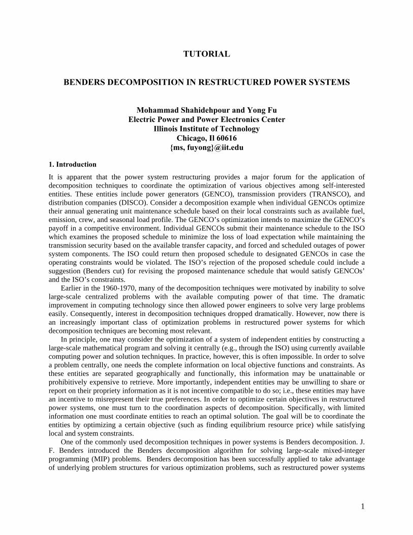
Fig. 1.1 depicts the hierarchy for calculating security-constrained unit commitment (SCUC) which is based on the existing set up (GENCOs and TRANSCOs as separate entities) in restructured power systems. The hierarchy utilizes a Benders decomposition which decouples the SCUC into a master problem (optimal generation scheduling) and network security check subproblems. The output of the master problem is the on/off state of units which are examined in the subproblem for satisfying the network constraints. The network violations are formulated in the form of Benders cuts which ate are added to the optimal generation scheduling formulation for re-calculating the original unit commitment solution.
GENCOs TRANSCOs
Master Problem (Optimal Generation)
Subproblem (Network Security Check)
Cuts UC
Schedules
DISCOs
Fig. 1.1 ISO and market participants
Other applications of Benders decomposition to security-constrained power systems include:
• Generating Unit Planning • Transmission Planning • Optimal Generation Bidding and Valuation • Reactive Power Planning • Optimal Power Flow • Hydro-thermal Scheduling • Generation Maintenance Scheduling • Transmission Maintenance Scheduling • Long-term Fuel Budgeting and Scheduling • Long-term Generating Unit Scheduling and Valuation
2
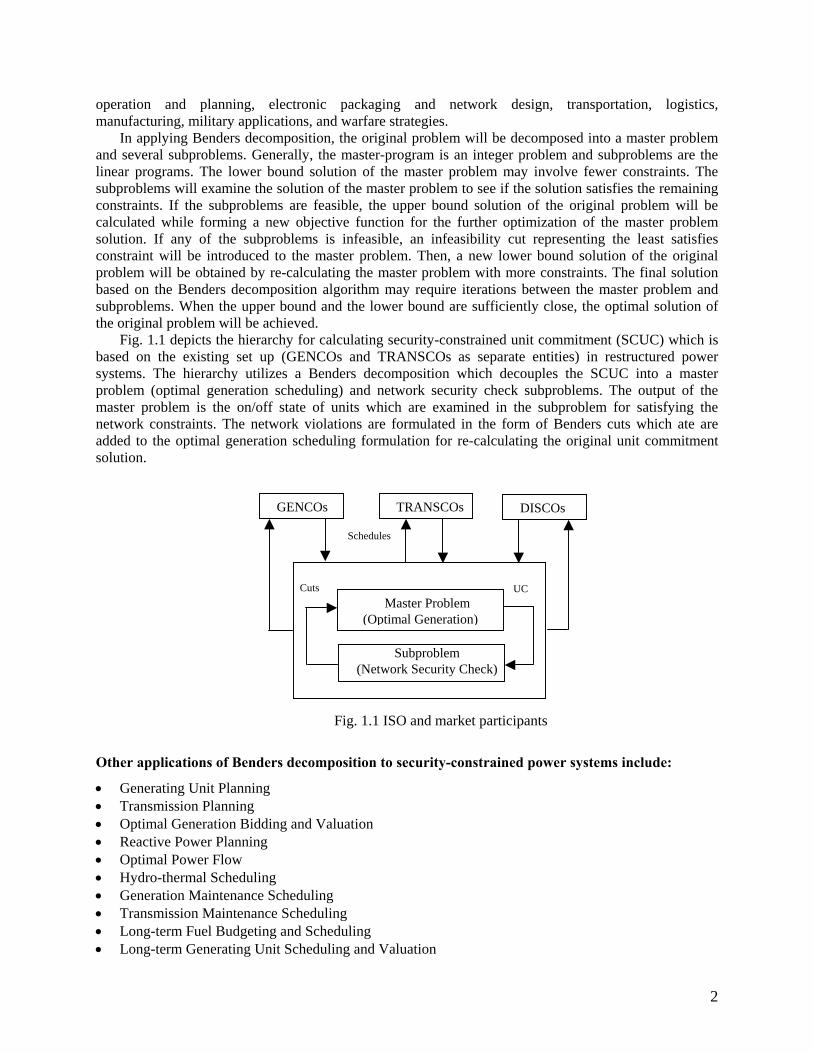
In order to discuss the applications of Benders decomposition to power systems, we review in the following the subject of duality in linear programs. 2. Primal and Dual Linear Programs
In this section, the relationship between primal and dual problems and the related duality theorems are discussed. Every linear program (LP), called the primal problem can be equivalently expressed in another LP form called the dual problem. The primal problem can be expressed in matrix notation as follows:
0xbAx
xcT
≥≥
=.. ts
zMinimize Primal (2.1)
where and are n-vector, is an m-vector and is an c x b A m x n matrix. The linear function is called
xcT
objective function. The linear inequalities are called constraints and they form a feasible region for minimizing the objective function. The solution elements of the primal problem in the feasible region is written as { }0xb,AxRx n ≥≥∈ . Also, its corresponding dual problem is defined as:
Dual (2.2) 0y
cyA
ybT
T
≥≤
=
.. ts
zMaximize
The number of inequalities in the primal problem becomes the number of variables in the dual problem. Correspondingly, the number of variables in the primal problem becomes the number of inequalities in the dual problem. Hence the dual problem differs in dimensions from the primal problem. It is typically easier to solve an LP with fewer constraints. Since the primal problem has m constraints while the dual problem has n constraints, this generates the following rule of thumb: Solve the LP problem that has the fewer number of constraints. For instance, solve the primal problem if m<n, but solve the dual problem if m>n. The relationship between primal and dual problems is listed in Table 2.1.
Table 2.1 Primal (or Dual) Dual (or Primal)
Objective zMax wMin Objective 0≥ ≥ 0≤ ≤
Variable (n)
Unlimited =
Constraints (n)
≤ 0≥ ≥ 0≤
Constraints (m)
= Unlimited
Variable (m)
Right-side vector of constraints Coefficients of variables in objective function Coefficients of variables in objective function Right-side vector of constraints
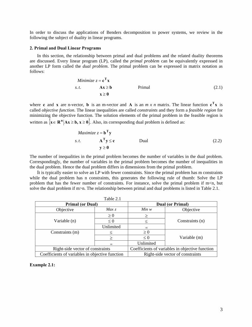
Example 2.1:
3
Primal problem Dual problem
itedunxxxxxxxxx
xxxxtS
xxxzMax
lim,0,01
523322..
645
321
321
321
31
21
321
≤≥
=+−−≤++−
≤+≥+
++=
itedunyyyyyyyyyyyyyytS
yyyywMin
lim,0,,0642253..
532
4321
432
431
4321
4321
≥≤=++≤−+
≥+−++−+=
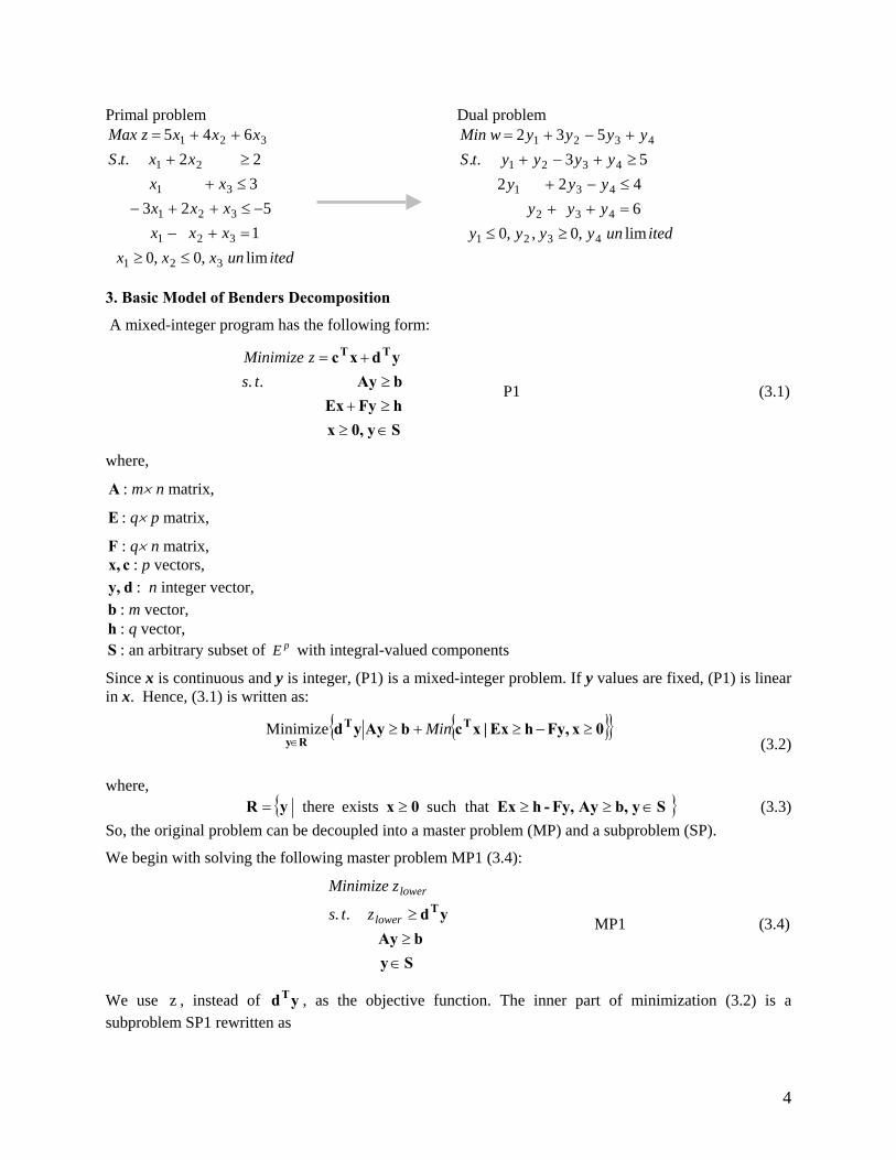
3. Basic Model of Benders Decomposition
A mixed-integer program has the following form:
P1 (3.1)
Sy0,xhFyExbAyydxc TT
∈≥≥+≥
+=.. ts
zMinimize
where,
A : m× n matrix,
E : q× p matrix,
F : q× n matrix, cx, : p vectors, dy, : n integer vector,
b : m vector, h : q vector, S : an arbitrary subset of pE with integral-valued components
Since x is continuous and y is integer, (P1) is a mixed-integer problem. If y values are fixed, (P1) is linear in x. Hence, (3.1) is written as:
{ }{ }0xFy,hEx|xcbAyyd TTRy
≥−≥+≥∈
Min Minimize (3.2)
where, { }Syb,AyFy,-hEx0xyR ∈≥≥≥= that such exists there (3.3)
So, the original problem can be decoupled into a master problem (MP) and a subproblem (SP).
We begin with solving the following master problem MP1 (3.4):
MP1 (3.4)
SybAy
ydT
∈≥≥lower
lower
zts
zMinimize
..
We use , instead of , as the objective function. The inner part of minimization (3.2) is a subproblem SP1 rewritten as
z ydT
4
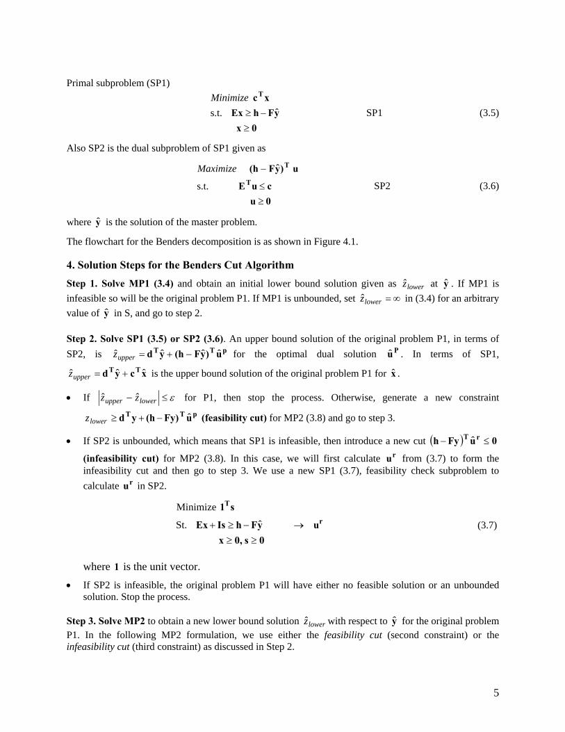
Primal subproblem (SP1)
0xyFhEx
xcT
≥−≥
ˆ s.t.
Minimize SP1 (3.5)
Also SP2 is the dual subproblem of SP1 given as
SP2 (3.6) 0ucuE
u)yF(h T
T
≥≤
−
s.t.
ˆMaximize
where is the solution of the master problem. y
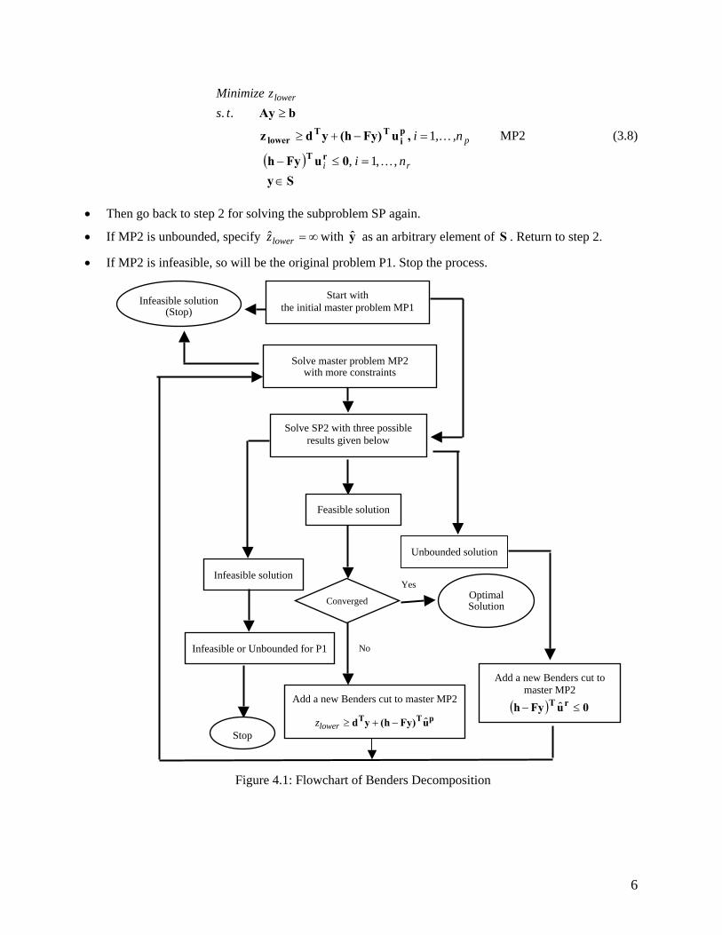
The flowchart for the Benders decomposition is as shown in Figure 4.1.
4. Solution Steps for the Benders Cut Algorithm
Step 1. Solve MP1 (3.4) and obtain an initial lower bound solution given as at y . If MP1 is infeasible so will be the original problem P1. If MP1 is unbounded, set
lowerz ˆ∞=lowerz in (3.4) for an arbitrary
value of in S, and go to step 2. y Step 2. Solve SP1 (3.5) or SP2 (3.6). An upper bound solution of the original problem P1, in terms of SP2, is for the optimal dual solution . In terms of SP1,
is the upper bound solution of the original problem P1 for .
pTT u)yF(h yd ˆˆˆˆ −+=upperz Pu
xc yd TT ˆˆˆ +=upperz x
• If ε≤− lowerupper zz ˆˆ for P1, then stop the process. Otherwise, generate a new constraint
(feasibility cut) for MP2 (3.8) and go to step 3. pTT uFy)(hyd ˆ−+≥lowerz
• If SP2 is unbounded, which means that SP1 is infeasible, then introduce a new cut
(infeasibility cut) for MP2 (3.8). In this case, we will first calculate from (3.7) to form the infeasibility cut and then go to step 3. We use a new SP1 (3.7), feasibility check subproblem to calculate in SP2.
( ) 0uFyh rT ≤− ˆru
ru
(3.7) 0s0,x
uyFhIsEx
s1 r
T
≥≥→−≥+ ˆ St.
Minimize
where 1 is the unit vector. • If SP2 is infeasible, the original problem P1 will have either no feasible solution or an unbounded
solution. Stop the process. Step 3. Solve MP2 to obtain a new lower bound solution with respect to y for the original problem P1. In the following MP2 formulation, we use either the feasibility cut (second constraint) or the infeasibility cut (third constraint) as discussed in Step 2.
lowerz ˆ
5
MP2 (3.8)
( )Sy
0uFyh
,uFy)(hydz
bAy
rT
pi
TTlower
∈=≤−
=−+≥
≥
ri
p
lower
ni
,n,i
tszMinimize
,,1,
1
..
K
K
• Then go back to step 2 for solving the subproblem SP again.
• If MP2 is unbounded, specify ∞=lowerz with as an arbitrary element of . Return to step 2. y S
• If MP2 is infeasible, so will be the original problem P1. Stop the process.
No
Yes
Add a new Benders cut to master MP2
( ) 0uFyh rT ≤− ˆ
Start with the initial master problem MP1
Solve master problem MP2 with more constraints
Solve SP2 with three possible results given below
Add a new Benders cut to master MP2
pTT uFy)(hyd ˆ−+≥lowerz
Feasible solution
Unbounded solution
Infeasible solution
Infeasible or Unbounded for P1
Converged
Stop
Optimal Solution
Infeasible solution (Stop)
Figure 4.1: Flowchart of Benders Decomposition
6
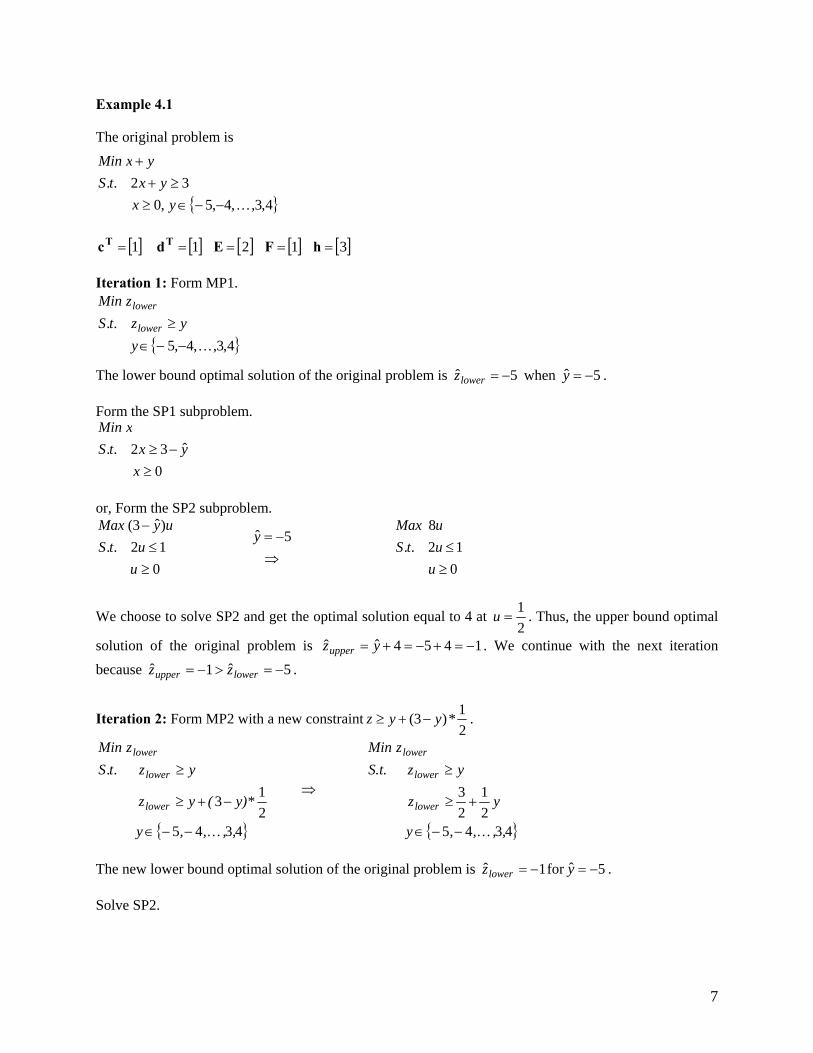
Example 4.1
The original problem is
{ }4,3,,4,5,032..
K−−∈≥≥+
+
yxyxtS
yxMin
[ ]1=Tc [ ]1=Td [ ]2=E [ ]1=F [ ]3=h
Iteration 1: Form MP1.
{ }4,3,,4,5..
K−−∈≥
yyztS
zMin
lower
lower
The lower bound optimal solution of the original problem is 5ˆ −=lowerz when . 5ˆ −=y
Form the SP1 subproblem.
0ˆ32..
≥−≥
xyxtS
xMin
or, Form the SP2 subproblem.
012..)ˆ3(
≥≤
−
uutS
uyMax
⇒−= 5y
012..
8
≥≤
uutSuMax
We choose to solve SP2 and get the optimal solution equal to 4 at 21
=u . Thus, the upper bound optimal
solution of the original problem is 1454ˆˆ −=+−=+= yzupper . We continue with the next iteration because . 5ˆ1ˆ −=>−= lowerupper zz
Iteration 2: Form MP2 with a new constraint21*)3( yyz −+≥ .
{ }4345213
..
,,,,y
y)*(y z
yztSzMin
lower
lower
lower
K−−∈
−+≥
≥ ⇒
{ }434521
23
,,,,y
y z
y zS.t.zMin
lower
lower
lower
K−−∈
+≥
≥
The new lower bound optimal solution of the original problem is 1ˆ −=lowerz for . 5ˆ −=y
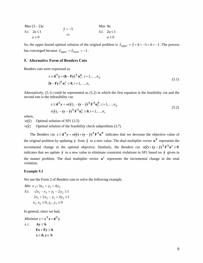
Solve SP2.
7
012..)ˆ3(
≥≤
−
uutS
uyMax
⇒−= 5y
012..
8
≥≤
uutSuMax
So, the upper bound optimal solution of the original problem is 1454ˆˆ −=+−=+= yzupper . The process has converged because 1ˆˆ −== lowerupper zz .
5. Alternative Form of Benders Cuts
Benders cuts were expressed as
(5.1) ( ) ri
pi
ni
niz
,,1,
,,1,
K
K
=≤−
=−+≥
0uFyh
uFy)(hydrT
pTT
Alternatively, (5.1) could be represented as (5.2) in which the first equation is the feasibility cut and the second one is the infeasibility cut.
ri
pi
niv
niwz
,,1,ˆ)ˆ(
,,1,ˆ)ˆ(
K
K
=≤−−
=−−+≥
0uF)y(yy
uF)y(yyydri
TT
Pi
TTT
(5.2)
where, )ˆ(yw Optimal solution of SP1 (3.5) )ˆ(yv Optimal solution of the feasibility check subproblem (3.7)
The Benders cut indicates that we decrease the objective value of
the original problem by updating from to a new value. The dual multiplier vector represents the
incremental change in the optimal objective. Similarly, the Benders cut indicates that we update y to a new value to eliminate constraint violations in SP1 based on given in
the master problem. The dual multiplier vector represents the incremental change in the total violation.
PTTT uF)y(y)y(yd ˆˆ −++≥ wz
y y Pu
0uF)y(y)y( rTT ≤−+ ˆˆvˆ y
ru
Example 5.1
We use the Form 2 of Benders cuts to solve the following example.
0,0,1322122
43
2121
2121
2121
2121
≥≥≥+−+≥−+−
+++
yy,xxyyxx yyxxS.t. -
yyxMin x
In general, since we had,
Sy0,xhFyEx
bAyydxc TT
∈≥≥+
≥+=
.. tszMinimize
8
Accordingly, for the above example,
4] [1 3] [1 == TT dc ⎥⎦
⎤⎢⎣
⎡ −−=
2212
E ⎥⎦
⎤⎢⎣
⎡−
−=
3121
F ⎥⎦
⎤⎢⎣
⎡=
11
h
Iteration 1: Solve MP1
0,0..
21 ≥≥+≥
yy4yyz tS
z inM
21lower
lower
which results in 0z0,y 0,y lower21 === ˆˆˆ . We use the feasibility check subproblem (3.7) because SP2 is unbounded at . 0y 0,y 21 == ˆˆ
s,s,x,xu yysxx
u yysxxSt. sMin s
00ˆ3ˆ122ˆ2ˆ12
2121
221221
121121
21
≥≥−+≥+++−≥+−−
+
The optimal solution is 1.5 and its dual multipliers are 5.0ˆ,0.1ˆ 21 == uu . The Benders cut is 30)ˆ(*5.0)ˆ(*5.05.1 212211 ≥−⇒≤−+−− yyyyyy at 0y 0,y 21 == ˆˆ .
Iteration 2: The new master problem MP2 is
03
4
21
21
21
≥≥−
+≥
y,y yy
yyzS.t.zMin
lower
lower
Hence, the new lower bound optimal solution of the original problem is for3ˆ =lowerz 0y ,y 21 == ˆ3ˆ . We form the primal subproblem SP1 as
x,xu yyxx
u yyxxSt. xMin x
0ˆ3ˆ122ˆ2ˆ12
3
21
22121
12121
21
≥−+≥++−≥−−
+
Here SP1 is feasible with an optimal solution equal to 6 and dual multipliers equal to 5.2ˆ,0.2ˆ 21 == uu . The feasibility cut is )ˆ(*5.3)ˆ(*5.064 221121 yyyyyyzlower −−−+++≥ . So . Accordingly, the upper bound solution of the original problem is
. We will continue the process because 21 5.05.15.4 yyzlower ++≥9636ˆ4ˆˆ 21 =+=++= yyzupper 3ˆ9ˆ =>= lowerupper zz .
Iteration 3: Add to MP2. So, 21 5.05.15.4 yyzlower ++≥
9
03
5.05.15.44
21
21
21
21
≥≥−
++≥+≥
y,y yy
yyz yyzS.t.
zMin
lower
lower
lower
Hence, the new lower bound solution of the original problem is 9ˆ =lowerz when . 0y ,y 21 == ˆ3ˆSolve SP1. The optimal solution is 6 and 9636ˆ4ˆˆ 21 =+=++= yyzupper . We terminate the iterative optimization process because 9ˆˆ == lowerupper zz .
6. Benders Decomposition for Security-Constrained Unit Commitment (SCUC) In order to apply Benders decomposition to SCUC, we write the SCUC problem as a standard Benders formulation. The startup cost of unit i is expressed as itist α where is the startup cost and ist itα is a binary variable that is equal to 1 if unit i is started up at hour t and is 0 otherwise. The shutdown cost is expressed similarly as itisd β where is the shutdown cost of unit i and isd itβ is a binary variable that is equal to 1 if unit i is shut down at hour t and is 0 otherwise. The production cost is proportional to the unit output power which is expressed as where is the cost coefficient of unit i and is the generated power of unit i at hour t. Thus, the objective of SCUC is written as:
iti pc ic itp
(6.1) ∑=
∑=
++=T
t
NG
iitiitiiti sdstpcZMin
1 1βα
A unit that is online can be shut down but not started up. Similarly, a unit that is offline can be started up but not shut down. This can be expressed as
)1( −−=− tiititit IIβα . (6.2)
where is a binary variable that is equal to 1 if unit i is online during hour t and is 0 otherwise. itI For the first hour, the above constraint becomes 0111 iiii II −=− βα where is the initial state of unit i. Its value is 1 if unit i is online at the initial hour and is 0 otherwise. The minimum up/down time limits of a unit are given as:
0iI
),,2()1(*
)1,,1(*
min,
min,
1
min,min,
NTTNTttNTI
TNTtTI
oni
NT
titit
oni
Tt
t
oniitit
oni
L
L
+−=+−≥
+−=≥
∑
∑−+
α
α
(6.3) ),,2()1(*]1[
)1,,1(*]1[
min,
min,
1
min,min,
NTTNTttNTI
TNTtTI
offi
NT
titit
offi
Tt
t
offiitit
offi
L
L
+−=+−≥−
+−=≥−
∑
∑−+
β
β
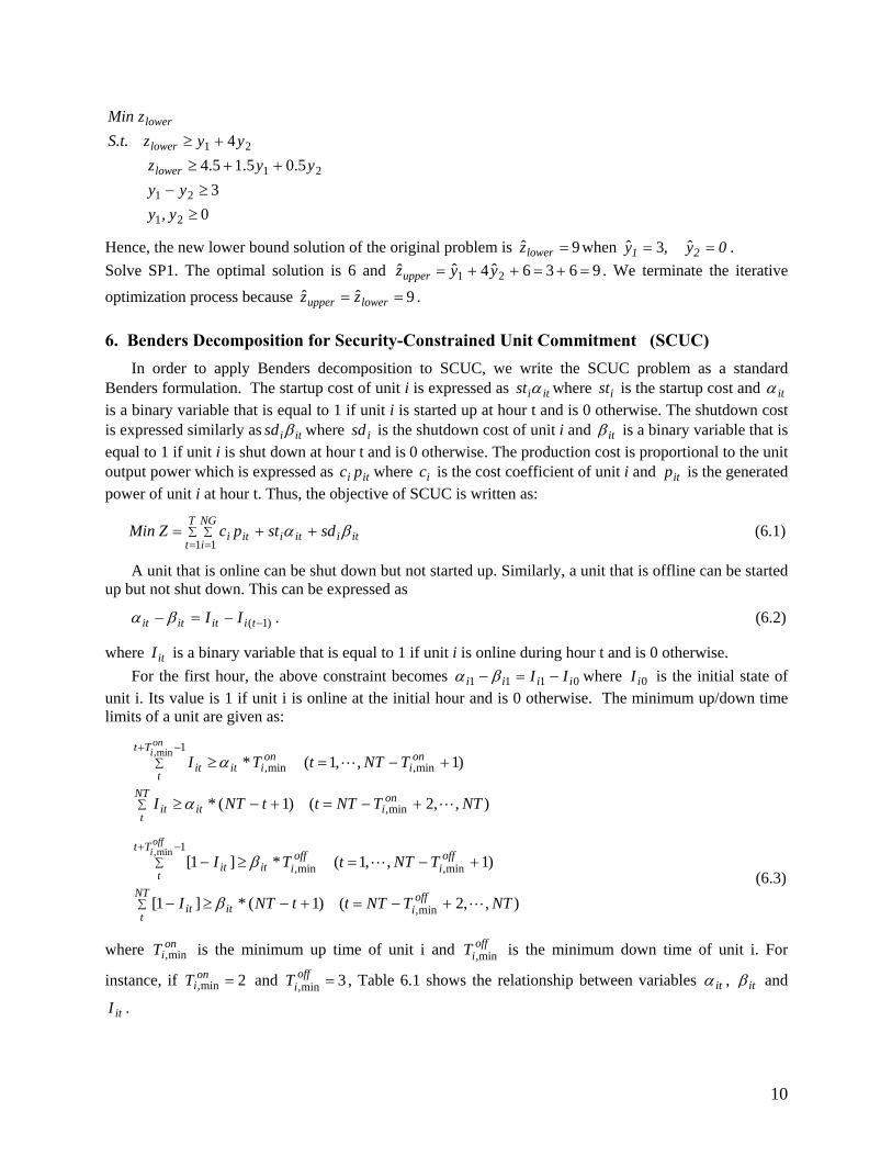
where is the minimum up time of unit i and is the minimum down time of unit i. For
instance, if and , Table 6.1 shows the relationship between variables
oniT min,
offiT min,
2min, =oniT 3min, =off
iT itα , itβ and
. itI
10
Table 6.1 Relationship among itα , itβ and itIHours 0 1 2 3 4 5 6 7 8 9 10
The additional constraints are given as System reserve requirements
(6.4) tNG
ititi RDIp +≥∑
=1max,
where NG is the number of units, is the demand in hour t, and is system reserve at hour t. tD tR
Hourly power demand
(6.5) ∑=
=NG
itit Dp
1
Thermal unit capacity constraint
(6.6) itiititi IPpIP max,min, ≤≤
Hourly network constraint
(6.7) max,,max, )( kmtkmkm PLfPL ≤≤− pI,where is the power flow on the line extending from bus k to bus m and is the line capacity. kmf max,kmPL
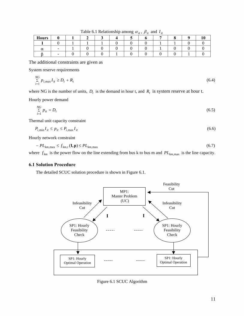
6.1 Solution Procedure The detailed SCUC solution procedure is shown in Figure 6.1.
MP1: Master Problem
(UC)
SP1: Hourly Feasibility
Check
SP1: Hourly Feasibility
Check
Feasibility Cut
Infeasibility Cut
I I
SP1: Hourly Optimal Operation
SP1: Hourly Optimal Operation
Infeasibility Cut
Figure 6.1 SCUC Algorithm
11
The initial SCUC master problem (MP1) is formulated as
(6.8) ∑=
∑=
+≥T
t
NG
iitiitilower
lower
sdstZ
ZMin
1 1βα
S.t.
additional constraints (6.2)-(6.4).
In this case, SP1 consists of the following two processes as shown in Figure 6.1.
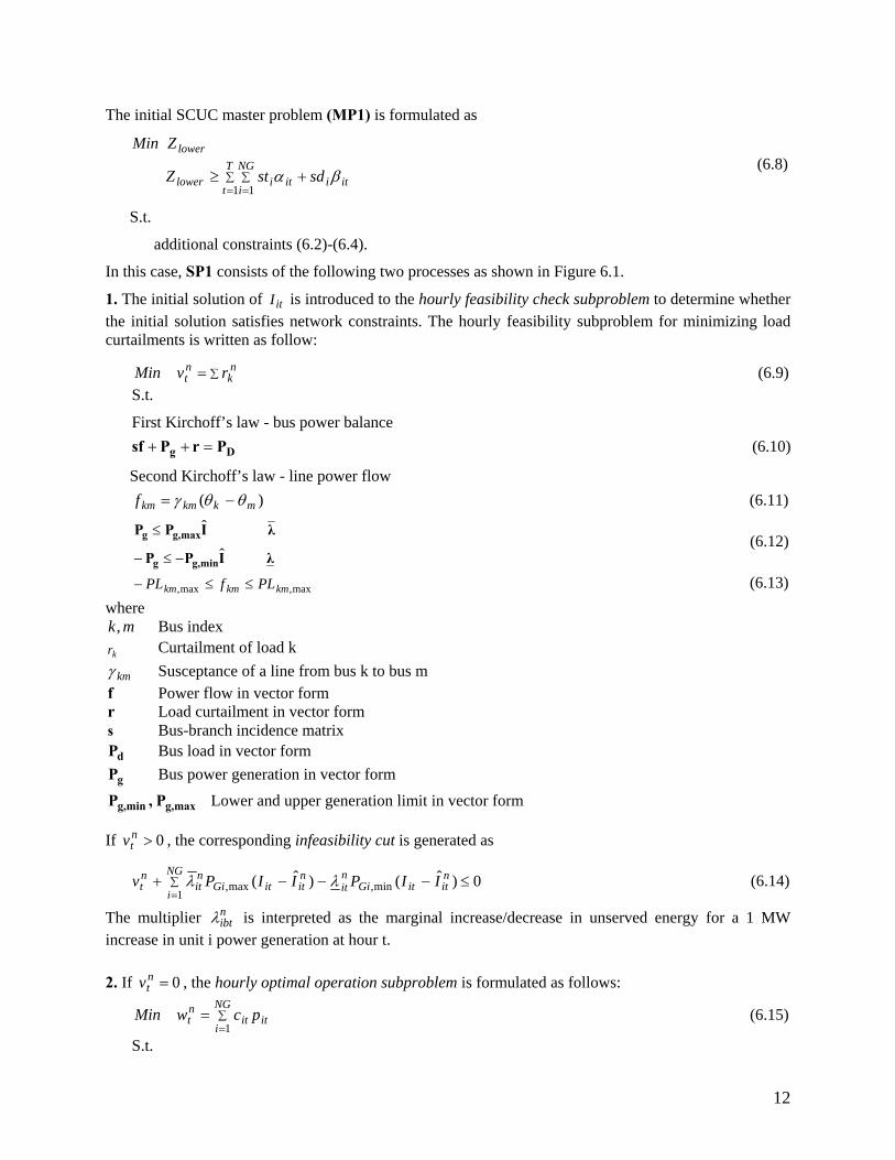
1. The initial solution of is introduced to the hourly feasibility check subproblem to determine whether the initial solution satisfies network constraints. The hourly feasibility subproblem for minimizing load curtailments is written as follow:
itI
(6.9) ∑= nk
nt rvMin
S.t.
First Kirchoff’s law - bus power balance (6.10) Dg PrPsf =++
Second Kirchoff’s law - line power flow )( mkkmkmf θθγ −= (6.11)
λIPP
λIPP
ming,g
maxg,g
ˆ
ˆ
−≤−
≤ (6.12)
(6.13) max,max, kmkmkm PLfPL ≤≤−
where mk, Bus index
kr Curtailment of load k
kmγ Susceptance of a line from bus k to bus m f Power flow in vector form r Load curtailment in vector form s Bus-branch incidence matrix
dP Bus load in vector form
gP Bus power generation in vector form
g,maxg,min P,P Lower and upper generation limit in vector form
If , the corresponding infeasibility cut is generated as 0>ntv
0)ˆ()ˆ( min,1
max, ≤−−−+ ∑=
nititGi
nit
NG
i
nititGi
nit
nt IIPIIPv λλ (6.14)
The multiplier is interpreted as the marginal increase/decrease in unserved energy for a 1 MW increase in unit i power generation at hour t.
nibtλ
2. If , the hourly optimal operation subproblem is formulated as follows: 0=n
tv
(6.15) ∑=
=NG
iitit
nt pcwMin
1 S.t.
12
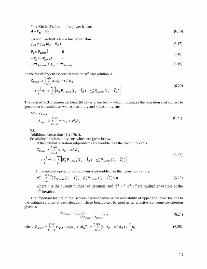
First Kirchoff’s law — bus power balance (6.16) Dg PPsf =+
Second Kirchoff’s law – line power flow )( mkkmkmf θθγ −= (6.17)
πIPP
πIPP
ming,g
maxg,g
ˆ
ˆ
−≤−
≤ (6.18)
(6.19) max,max, kmkmkm PLfPL ≤≤−
So the feasibility cut associated with the nth trial solution is
[ ]∑ ∑
=
∑=
∑=
⎭⎬⎫
⎩⎨⎧ −−−++
+≥
t
NG
i
nititGi
nit
nititGi
nit
nt
T
t
NG
iitiitilower
IIPIIPw
sdstZ
1min,max,
1 1
)ˆ()ˆ( ππ
βα (6.20)
The revised SCUC master problem (MP2) is given below which minimizes the operation cost subject to generation constraints as well as feasibility and infeasibility cuts.
(6.21) ∑=
∑=
+≥T
t
NG
iitiitilower
lower
sdstZ
ZMin
1 1βα
S.t. Additional constraints (6.2)-(6.4). Feasibility or infeasibility cuts which are given below: If the optimal operation subproblems are feasible then the feasibility cut is
[ ]∑ ∑
=
∑=
∑=
⎭⎬⎫
⎩⎨⎧ −−−++
+≥
t
NG
i
nititGi
nit
nititGi
nit
nt
T
t
NG
iitiitilower
IIPIIPw
sdstZ
1min,max,
1 1
)ˆ()ˆ( ππ
βα (6.22)
If the optimal operation subproblem is infeasible then the infeasibility cut is:
0)ˆ()ˆ( min,1
max, ≤−−−+ ∑=
nititGi
nit
NG
i
nititGi
nit
nt IIPIIPv λλ (6.23)
where n is the current number of iteration, and nnnn πλπλ ,,, are multiplier vectors at the nth iteration.
The important feature of the Benders decomposition is the availability of upper and lower bounds to the optimal solution at each iteration. These bounds can be used as an effective convergence criterion given as
( )( ) ∆≤+
−lowerupper
lowerupperZZ
ZZ2 (6.24)
where (6.25) ∑=
∑=
∑=
∑=
∑=
++=++=T
t
NG
i
T
ttitiiti
T
t
NG
iitiitiitiupper wsdstsdstpcZ
1 1 11 1)( βαβα
13
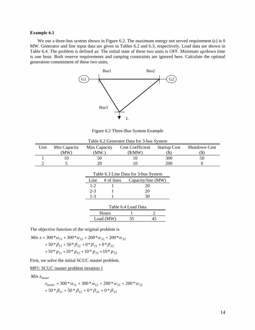
Example 6.1
We use a three-bus system shown in Figure 6.2. The maximum energy not served requirement (ε) is 0 MW. Generator and line input data are given in Tables 6.2 and 6.3, respectively. Load data are shown in Table 6.4. The problem is defined as: The initial state of these two units is OFF. Minimum up/down time is one hour. Both reserve requirements and ramping constraints are ignored here. Calculate the optimal generation commitment of these two units.
Bus1 Bus2
Bus3
L
G2G1
Figure 6.2 Three-Bus System Example
Table 6.2 Generator Data for 3-bus System Unit Min Capacity
(MW) Max Capacity
(MW.) Cost Coefficient
($/MW) Startup Cost
($) Shutdown Cost
($) 1 10 50 10 300 50 2 5 20 10 200 0
Table 6.3 Line Data for 3-bus System Line # of lines Capacity/line (MW) 1-2 1 20 2-3 1 20 1-3 1 30
Table 6.4 Load Data Hours 1 2
Load (MW) 35 45
The objective function of the original problem is
22211211
22211211
22211211
*10*10*10*10*0*0*50*50
*200*200*300*300
pppp
zMin
++++++++
+++=ββββ
αααα
First, we solve the initial SCUC master problem.
MP1: SCUC master problem iteration 1
22211211
22211211
*0*0*50*50*200*200*300*300
ββββαααα
+++++++=lower
lower
zzMin
14
45*20*5035*20*50
0
0..
2212
2111
21222222
212121
11121212
111111
≥+≥+
−=−−=−−=−−=−
IIII
III
IIItS
βαβαβαβα
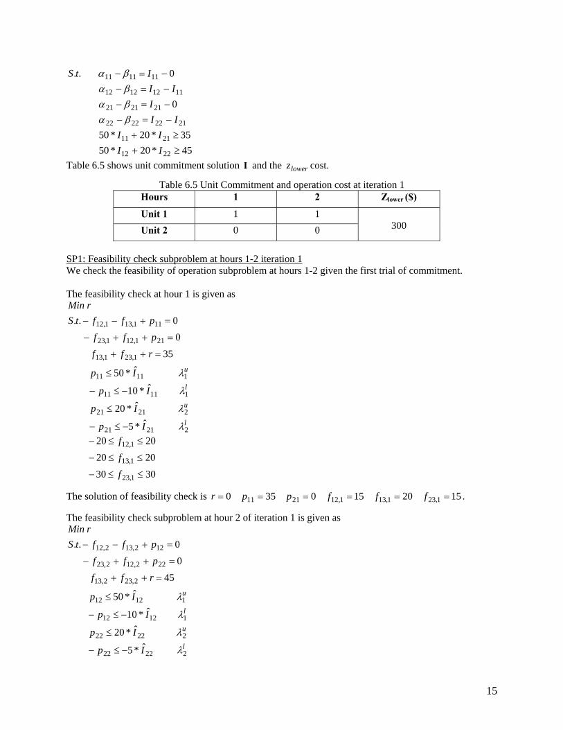
Table 6.5 shows unit commitment solution and the cost. I lowerz
Table 6.5 Unit Commitment and operation cost at iteration 1 Hours 1 2 Zlower ($)
Unit 1 1 1 Unit 2 0 0
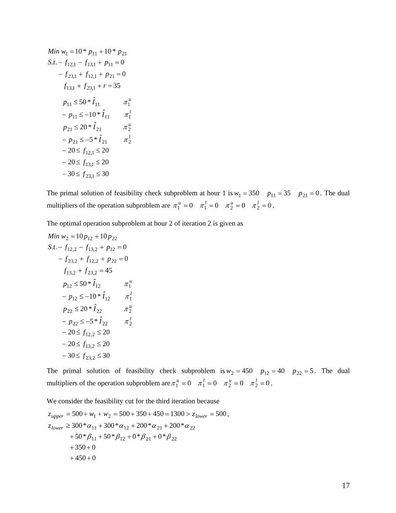
300
SP1: Feasibility check subproblem at hours 1-2 iteration 1 We check the feasibility of operation subproblem at hours 1-2 given the first trial of commitment. The feasibility check at hour 1 is given as
l
u
l
u
Ip
Ip
Ip
Ip
rff
pff
pfftSrMin
22121
22121
11111
11111
1,231,13
211,121,23
111,131,12
ˆ*5
ˆ*20
ˆ*10
ˆ*50
35
0
0..
λ
λ
λ
λ
−≤−
≤
−≤−
≤
=++
=++−
=+−−
3030
2020
2020
1,23
1,13
1,12
≤≤−
≤≤−
≤≤−
f
f
f
The solution of feasibility check is 1520150350 1,231,131,122111 ====== fffppr .
The feasibility check subproblem at hour 2 of iteration 1 is given as
l
u
l
u
Ip
Ip
Ip
Ip
rff
pff
pfftSrMin
22222
22222
11212
11212
2,232,13
222,122,23
122,132,12
ˆ*5
ˆ*20
ˆ*10
ˆ*50
45
0
0..
λ
λ
λ
λ
−≤−
≤
−≤−
≤
=++
=++−
=+−−
15
3030
2020
2020
2,23
2,13
2,12
≤≤−
≤≤−
≤≤−
f
f
f
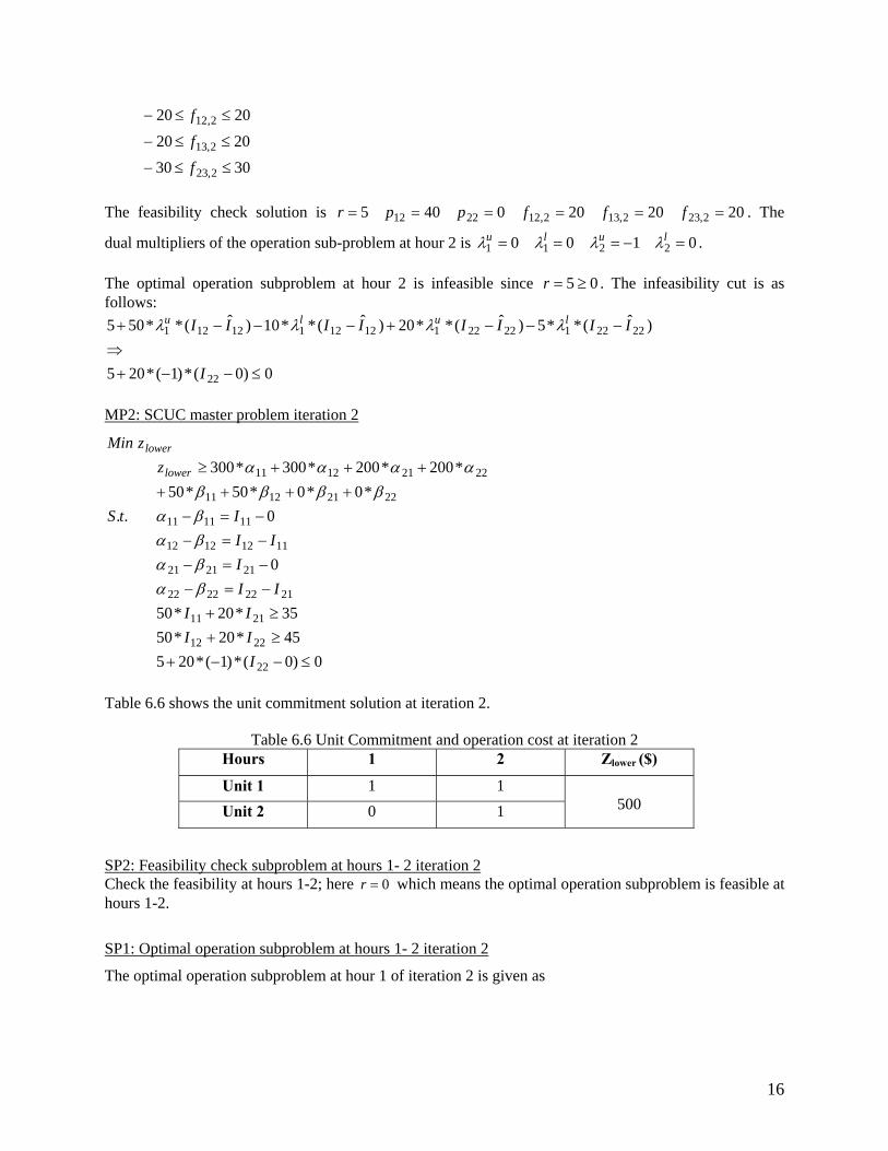
The feasibility check solution is 2020200405 2,232,132,122212 ====== fffppr . The
dual multipliers of the operation sub-problem at hour 2 is . 0100 2211 =−=== lulu λλλλ The optimal operation subproblem at hour 2 is infeasible since 05 ≥=r . The infeasibility cut is as follows:
0)0(*)1(*205
)ˆ(**5)ˆ(**20)ˆ(**10)ˆ(**505
22
22221222211212112121
≤−−+⇒
−−−+−−−+
I
IIIIIIII lulu λλλλ
MP2: SCUC master problem iteration 2
0)0(*)1(*20545*20*5035*20*50
0
0..*0*0*50*50
*200*200*300*300
22
2212
2111
21222222
212121
11121212
111111
22211211
22211211
≤−−+≥+≥+
−=−−=−−=−−=−
++++
+++≥
IIIII
III
IIItS
zzMin
lower
lower
βαβαβαβα
ββββαααα
Table 6.6 shows the unit commitment solution at iteration 2.
Table 6.6 Unit Commitment and operation cost at iteration 2
Hours 1 2 Zlower ($)
Unit 1 1 1 Unit 2 0 1
500
SP2: Feasibility check subproblem at hours 1- 2 iteration 2 Check the feasibility at hours 1-2; here 0=r which means the optimal operation subproblem is feasible at hours 1-2.
SP1: Optimal operation subproblem at hours 1- 2 iteration 2
The optimal operation subproblem at hour 1 of iteration 2 is given as
16
35
0
0..*10*10
1,231,13
211,121,23
111,131,12
21111
=++
=++−
=+−−+=
rff
pff
pfftSppwMin
3030
2020
2020
ˆ*5
ˆ*20
ˆ*10
ˆ*50
1,23
1,13
1,12
22121
22121
11111
11111
≤≤−
≤≤−
≤≤−−≤−
≤
−≤−
≤
f
f
fIp
Ip
Ip
Ip
l
u
l
u
π
π
π
π
The primal solution of feasibility check subproblem at hour 1 is 035350 21111 === ppw . The dual
multipliers of the operation subproblem are . 0000 2211 ==== lulu ππππ The optimal operation subproblem at hour 2 of iteration 2 is given as
3030
2020
2020
ˆ*5
ˆ*20
ˆ*10
ˆ*50
45
0
0..1010
2,23
2,13
2,12
22222
22222
11212
11212
2,232,13
222,122,23
122,132,12
22122
≤≤−
≤≤−
≤≤−−≤−
≤
−≤−
≤
=+
=++−
=+−−+=
f
f
fIp
Ip
Ip
Ip
ff
pff
pfftSppwMin
l
u
l
u
π
π
π
π
The primal solution of feasibility check subproblem is 540450 22122 === ppw . The dual
multipliers of the operation subproblem are . 0000 2211 ==== lulu ππππ We consider the feasibility cut for the third iteration because
Table 6.7 shows the unit commitment solution at iteration 3.
Table 6.7 Unit Commitment and operation cost at iteration 3 Hours 1 2 Zlower ($)
Unit 1 1 1 Unit 2 0 1
1300
It is obvious in next calculations and the final solution should be . 1300== upperlower zz 1300=z 7. Generation Resource Planning The objective function of the generation resource planning is to minimize the investment and operation cost while satisfying the system reliability. The objective function is formulated as follows:
( )[ ] ∑=
∑=
∑=
∑ ∑ − ∗+−=T
t
B
b
NG
iibtGibtbt
T
t
CG
itiitit POCDTXXCIYMin
1 1 1,)1( ** (7.1)
where i Existing or candidate unit index b Load block index t Planning year index B Number of load blocks CG Number of candidate units T Planning horizon NG Number of committed units CIit Capital investment for candidate unit i in year t DTbt Duration of load block b in year t OCibt Operating cost unit i among committed units at load block b in year t
18
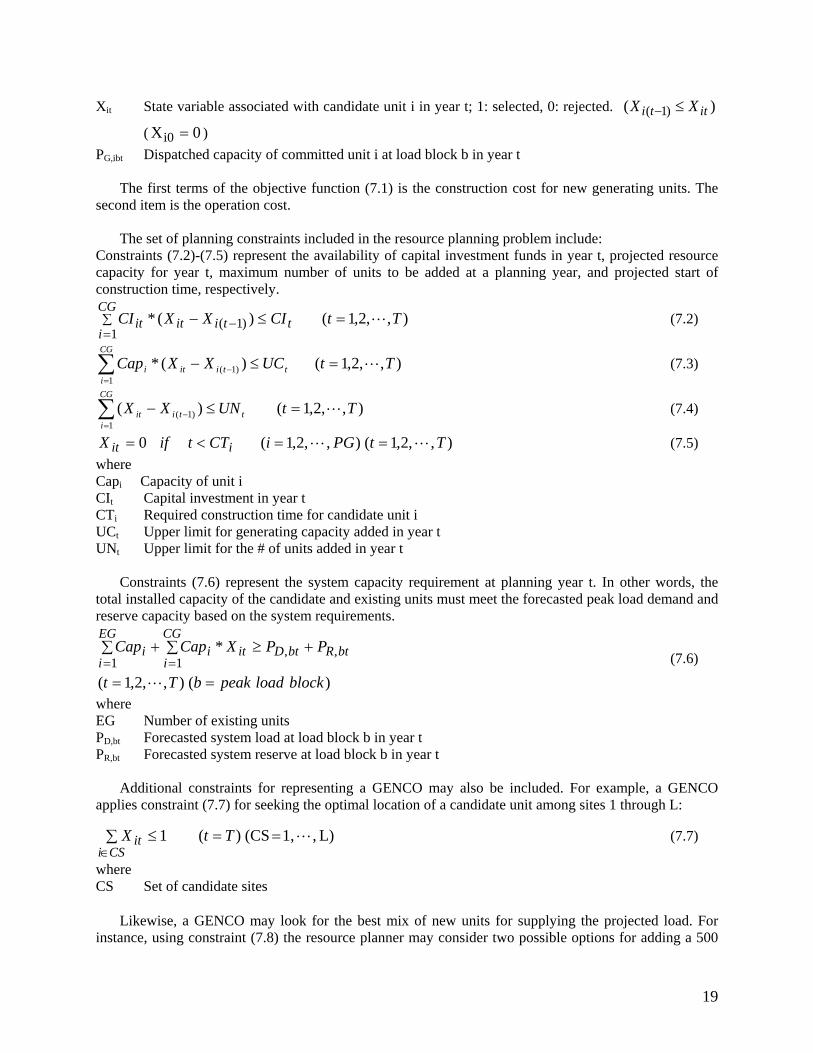
Xit State variable associated with candidate unit i in year t; 1: selected, 0: rejected. )( )1( itti XX ≤−
( ) 0Xi0 =PG,ibt Dispatched capacity of committed unit i at load block b in year t The first terms of the objective function (7.1) is the construction cost for new generating units. The second item is the operation cost. The set of planning constraints included in the resource planning problem include: Constraints (7.2)-(7.5) represent the availability of capital investment funds in year t, projected resource capacity for year t, maximum number of units to be added at a planning year, and projected start of construction time, respectively.
),,2,1()(*1
)1( TtCIXXCI tCG
itiitit L=≤−∑
=− (7.2)
),,2,1()(*1
)1( TtUCXXCap t
CG
itiiti L=≤−∑
=− (7.3)
),,2,1()(1
)1( TtUNXX t
CG
itiit L=≤−∑
=− (7.4)
),,2,1(),,2,1(0 TtPGiCTtifX iit LL ==<= (7.5) where Capi Capacity of unit i CIt Capital investment in year t CTi Required construction time for candidate unit i UCt Upper limit for generating capacity added in year t UNt Upper limit for the # of units added in year t Constraints (7.6) represent the system capacity requirement at planning year t. In other words, the total installed capacity of the candidate and existing units must meet the forecasted peak load demand and reserve capacity based on the system requirements.
)(),,2,1(
* ,,11
blockloadpeakbTt
PPXCapCap btRbtDCG
iiti
EG
ii
==
+≥∑+∑==
L
(7.6)
where EG Number of existing units PD,bt Forecasted system load at load block b in year t PR,bt Forecasted system reserve at load block b in year t Additional constraints for representing a GENCO may also be included. For example, a GENCO applies constraint (7.7) for seeking the optimal location of a candidate unit among sites 1 through L:
L),1, (CS)(1 L==≤∑∈
TtXCSi
it (7.7)
where CS Set of candidate sites Likewise, a GENCO may look for the best mix of new units for supplying the projected load. For instance, using constraint (7.8) the resource planner may consider two possible options for adding a 500
19
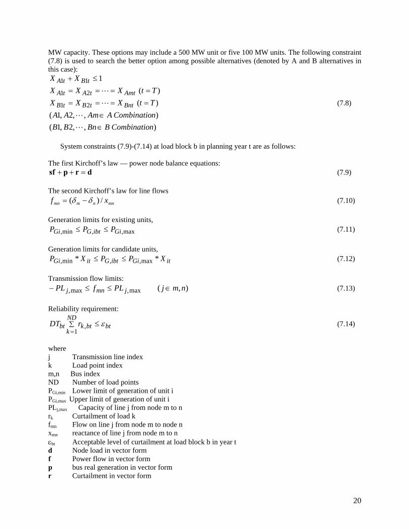
MW capacity. These options may include a 500 MW unit or five 100 MW units. The following constraint (7.8) is used to search the better option among possible alternatives (denoted by A and B alternatives in this case):
),,2,1(),,2,1()()(
1
21
21
11
nCombinatioBBnBBnCombinatioAAmAATtXXXTtXXX
XX
BnttBtB
AmttAtA
tBtA
∈∈
========
≤+
L
L
L
L
(7.8)
System constraints (7.9)-(7.14) at load block b in planning year t are as follows: The first Kirchoff’s law — power node balance equations:
drpsf =++ (7.9) The second Kirchoff’s law for line flows
where j Transmission line index k Load point index m,n Bus index ND Number of load points PGi,min Lower limit of generation of unit i PGi,max Upper limit of generation of unit i PLj,max Capacity of line j from node m to n rk Curtailment of load k fmn Flow on line j from node m to node n xmn reactance of line j from node m to n εbt Acceptable level of curtailment at load block b in year t d Node load in vector form f Power flow in vector form p bus real generation in vector form r Curtailment in vector form
20
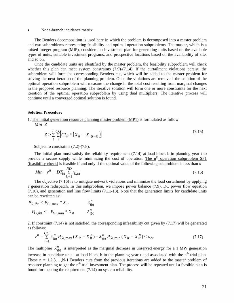
s Node-branch incidence matrix The Benders decomposition is used here in which the problem is decomposed into a master problem and two subproblems representing feasibility and optimal operation subproblems. The master, which is a mixed integer program (MIP), considers an investment plan for generating units based on the available types of units, suitable investment programs, and prospective locations based on the availability of site, and so on. Once the candidate units are identified by the master problem, the feasibility subproblem will check whether this plan can meet system constraints (7.9)-(7.14). If the curtailment violations persist, the subproblem will form the corresponding Benders cut, which will be added to the master problem for solving the next iteration of the planning problem. Once the violations are removed, the solution of the optimal operation subproblem will measure the change in the total cost resulting from marginal changes in the proposed resource planning. The iterative solution will form one or more constraints for the next iteration of the optimal operation subproblem by using dual multipliers. The iterative process will continue until a converged optimal solution is found.
Solution Procedure
1. The initial generation resource planning master problem (MP1) is formulated as follow:
(7.15) ([∑ ∑ −−≥T
t
CG
itiitit XXCIZ
ZMin
)1(* )] Subject to constraints (7.2)-(7.8).
The initial plan must satisfy the reliability requirement (7.14) at load block b in planning year t to provide a secure supply while minimizing the cost of operation. The nth operation subproblem SP1 (feasibility check) is feasible if and only if the optimal value of the following subproblem is less than ε
(7.16) ∑=
=ND
kbtkbt
n rDTvMin1
,
The objective (7.16) is to mitigate network violations and minimize the load curtailment by applying a generation redispatch. In this subproblem, we impose power balance (7.9), DC power flow equation (7.10), and generation and line flow limits (7.11-13). Note that the generation limits for candidate units can be rewritten as:
nibtitGiibtG
nibtitGiibtG
XPP
XPP
λ
λ
*
*
min,,
max,,
−≤−
≤
2. If constraint (7.14) is not satisfied, the corresponding infeasibility cut given by (7.17) will be generated as follows:
btnititGi
nibt
CG
i
nititGi
nibt
n XXPXXPv ελλ ≤−−−+ ∑=
)()( min,1
max, (7.17)
The multiplier nibtλ is interpreted as the marginal decrease in unserved energy for a 1 MW generation
increase in candidate unit i at load block b in the planning year t and associated with the nth trial plan. These n = 1,2,3,…,N-1 Benders cuts from the previous iterations are added to the master problem of resource planning to get the nth trial investment plan. The process will be repeated until a feasible plan is found for meeting the requirement (7.14) on system reliability.
21
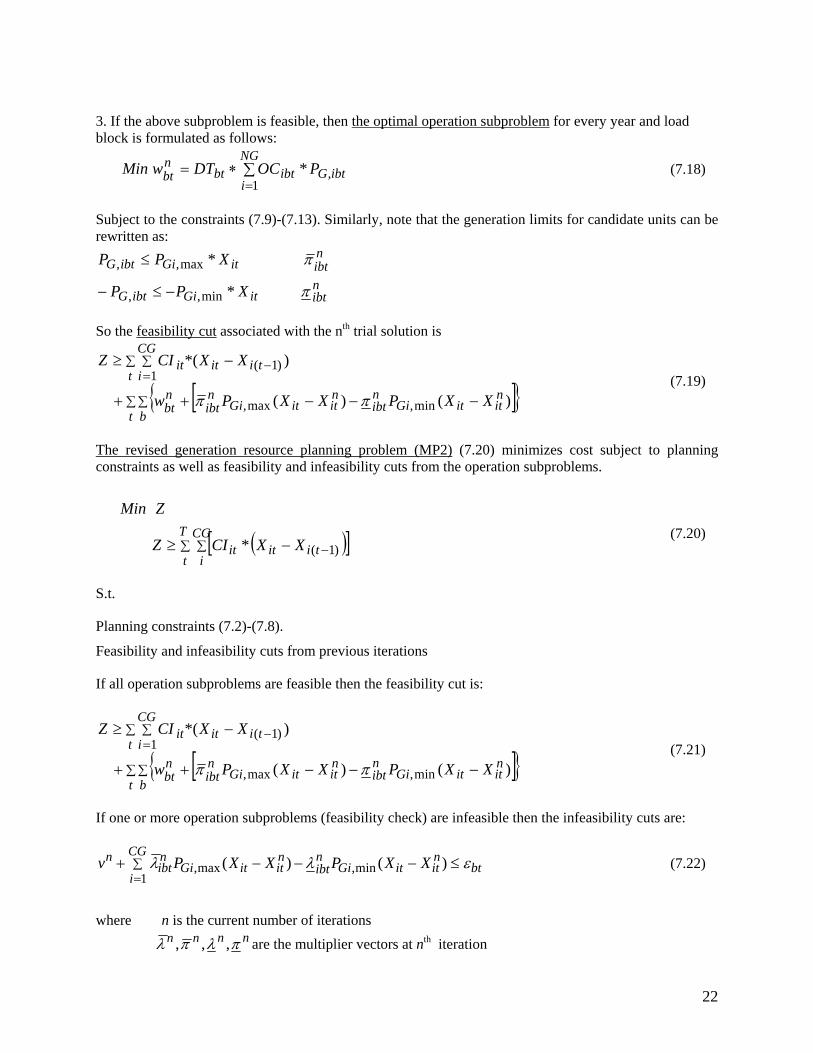
3. If the above subproblem is feasible, then the optimal operation subproblem for every year and load block is formulated as follows:
(7.18) ∑∗==
NG
iibtGibtbt
nbt POCDTwMin
1,*
Subject to the constraints (7.9)-(7.13). Similarly, note that the generation limits for candidate units can be rewritten as:
nibtitGiibtG
nibtitGiibtG
XPP
XPP
π
π
*
*
min,,
max,,
−≤−
≤
So the feasibility cut associated with the nth trial solution is
[ ]{ }∑ ∑
∑ ∑=
−
−−−++
−≥
t b
nititGi
nibt
nititGi
nibt
nbt
t
CG
itiitit
XXPXXPw
XXCIZ
)()(
)*(
min,max,
1)1(
ππ (7.19)
The revised generation resource planning problem (MP2) (7.20) minimizes cost subject to planning constraints as well as feasibility and infeasibility cuts from the operation subproblems.
( )[∑ ∑ −−≥T
t
CG
itiitit XXCIZ ]
ZMin
)1(* (7.20)
S.t.
Planning constraints (7.2)-(7.8).
Feasibility and infeasibility cuts from previous iterations
If all operation subproblems are feasible then the feasibility cut is:
[ ]{ }∑ ∑
∑ ∑=
−
−−−++
−≥
t b
nititGi
nibt
nititGi
nibt
nbt
t
CG
itiitit
XXPXXPw
XXCIZ
)()(
)*(
min,max,
1)1(
ππ (7.21)
If one or more operation subproblems (feasibility check) are infeasible then the infeasibility cuts are:
btnititGi
nibt
CG
i
nititGi
nibt
n XXPXXPv ελλ ≤−−−+ ∑=
)()( min,1
max, (7.22)
where n is the current number of iterations
nnnn πλπλ ,,, are the multiplier vectors at nth iteration
22
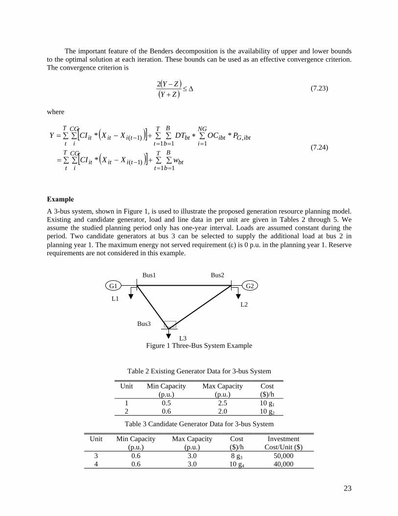
The important feature of the Benders decomposition is the availability of upper and lower bounds to the optimal solution at each iteration. These bounds can be used as an effective convergence criterion. The convergence criterion is
( )( ) ∆≤
+−ZYZY2 (7.23)
where
(7.24)
( )[ ]
( )[ ] ∑ ∑+∑ ∑ −=
∑ ∑ ∑∗+∑ ∑ −=
= =−
= = =−
T
t
B
bbt
T
t
CG
itiitit
T
t
B
b
NG
iibtGibtbt
T
t
CG
itiitit
wXXCI
POCDTXXCIY
1 1)1(
1 1 1,)1(
*
**
Example
A 3-bus system, shown in Figure 1, is used to illustrate the proposed generation resource planning model. Existing and candidate generator, load and line data in per unit are given in Tables 2 through 5. We assume the studied planning period only has one-year interval. Loads are assumed constant during the period. Two candidate generators at bus 3 can be selected to supply the additional load at bus 2 in planning year 1. The maximum energy not served requirement (ε) is 0 p.u. in the planning year 1. Reserve requirements are not considered in this example.
Figure 1 Three-Bus System Example
Table 2 Existing Generator Data for 3-bus System
Unit Min Capacity (p.u.)
Max Capacity (p.u.)
Cost ($)/h
1 0.5 2.5 10 g12 0.6 2.0 10 g2
Table 3 Candidate Generator Data for 3-bus System
Unit Min Capacity (p.u.)
Max Capacity (p.u.)
Cost ($)/h
Investment Cost/Unit ($)
3 0.6 3.0 8 g3 50,000 4 0.6 3.0 10 g4 40,000
Bus1 Bus2
G1 G2
L1 L2
Bus3
L3
23
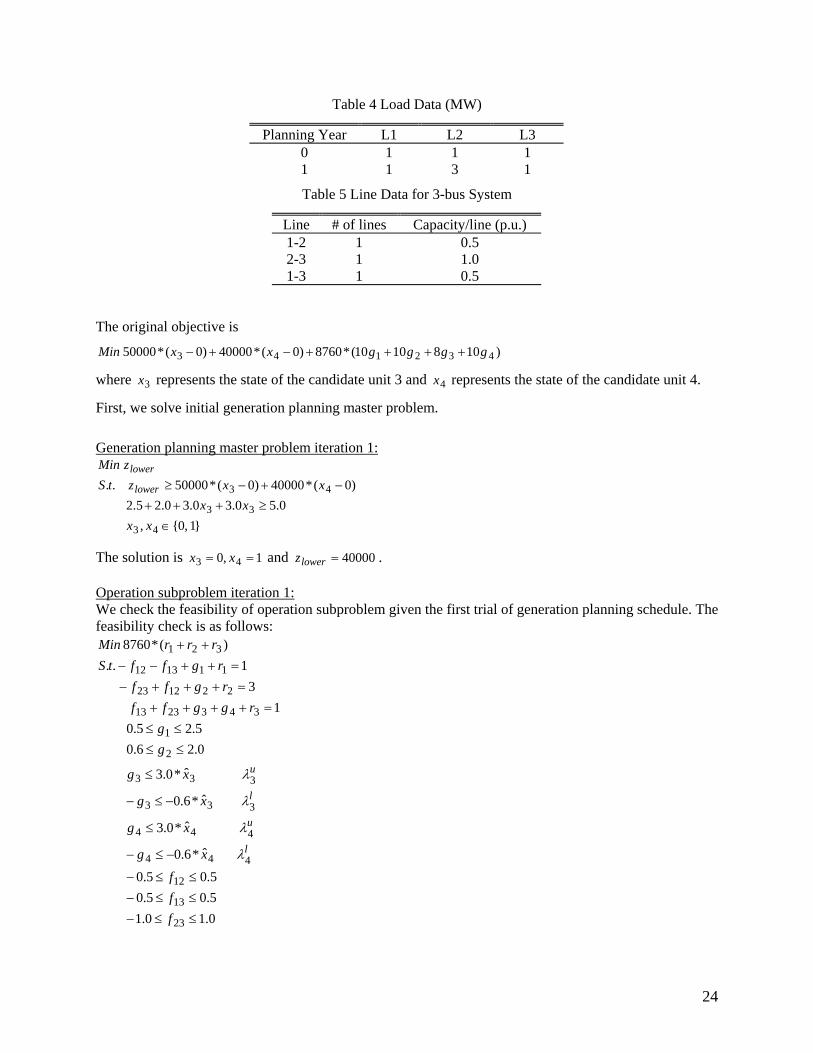
Table 4 Load Data (MW)
Planning Year L1 L2 L3 0 1 1 1 1 1 3 1
Table 5 Line Data for 3-bus System
Line # of lines Capacity/line (p.u.) 1-2 1 0.5 2-3 1 1.0 1-3 1 0.5
where represents the state of the candidate unit 3 and represents the state of the candidate unit 4. 3x 4x
First, we solve initial generation planning master problem.
Generation planning master problem iteration 1:
}1,0{,0.50.30.30.25.2
)0(*40000)0(*50000..
43
33
43
∈≥+++
−+−≥
xxxx
xxztSzMin
lower
lower
The solution is and 1,0 43 == xx 40000=lowerz .
Operation subproblem iteration 1: We check the feasibility of operation subproblem given the first trial of generation planning schedule. The feasibility check is as follows:
0.10.15.05.05.05.0
ˆ*6.0
ˆ*0.3
ˆ*6.0
ˆ*0.3
0.26.05.25.0
13
1..)(*8760
23
13
12
444
444
333
333
2
1
3432313
221223
111312
321
≤≤−≤≤−≤≤−
−≤−
≤
−≤−
≤
≤≤≤≤
=++++=+++−
=++−−++
fff
xg
xg
xg
xg
gg
rggffrgff
rgfftSrrrMin
l
u
l
u
λ
λ
λ
λ
24
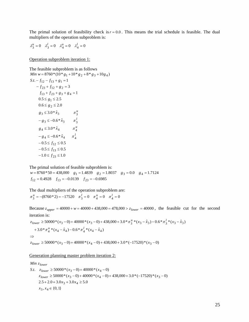
The primal solution of feasibility check is 0.0=r . This means the trial schedule is feasible. The dual multipliers of the operation subproblem is:
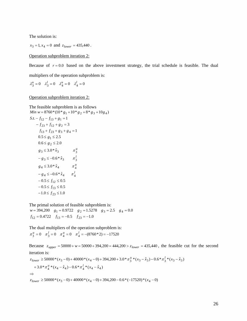
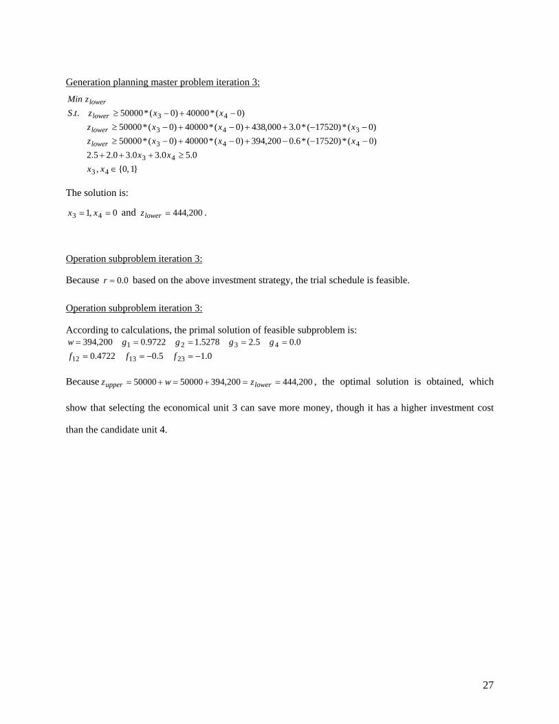
Because based on the above investment strategy, the trial schedule is feasible. 0.0=r
Operation subproblem iteration 3:
According to calculations, the primal solution of feasible subproblem is:
0.15.04722.00.05.25278.19722.0200,394
231312
4321−=−==
=====fff
ggggw
Because , the optimal solution is obtained, which
show that selecting the economical unit 3 can save more money, though it has a higher investment cost
than the candidate unit 4.
200,444200,3945000050000 ==+=+= lowerupper zwz
27
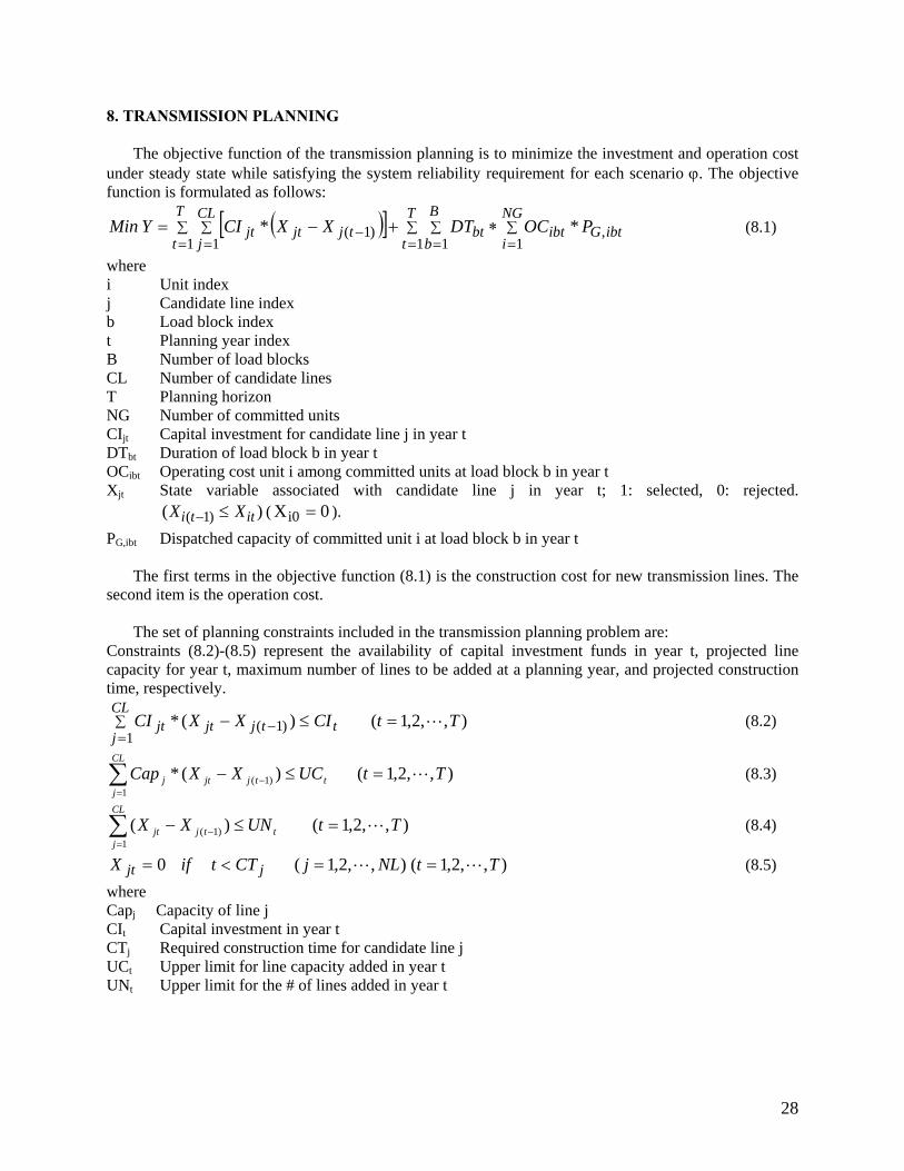
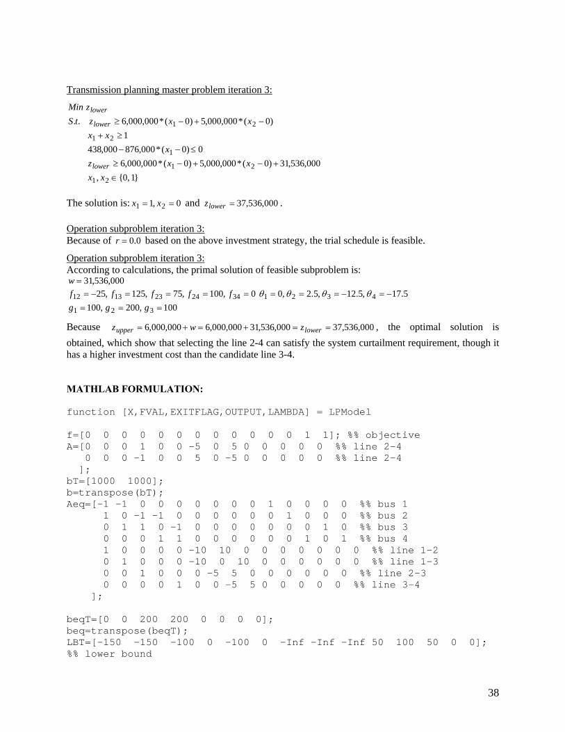
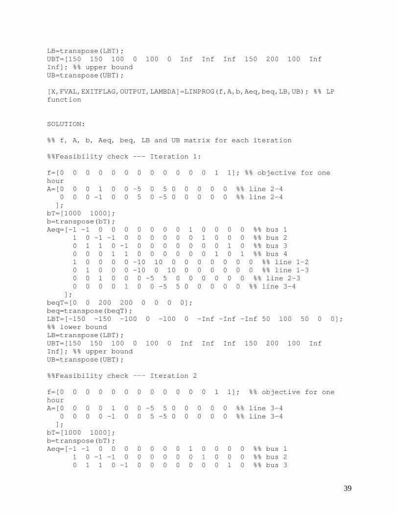
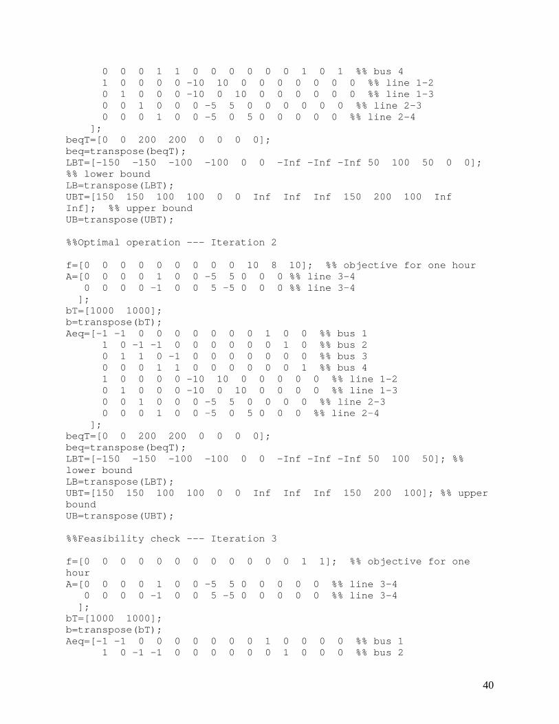
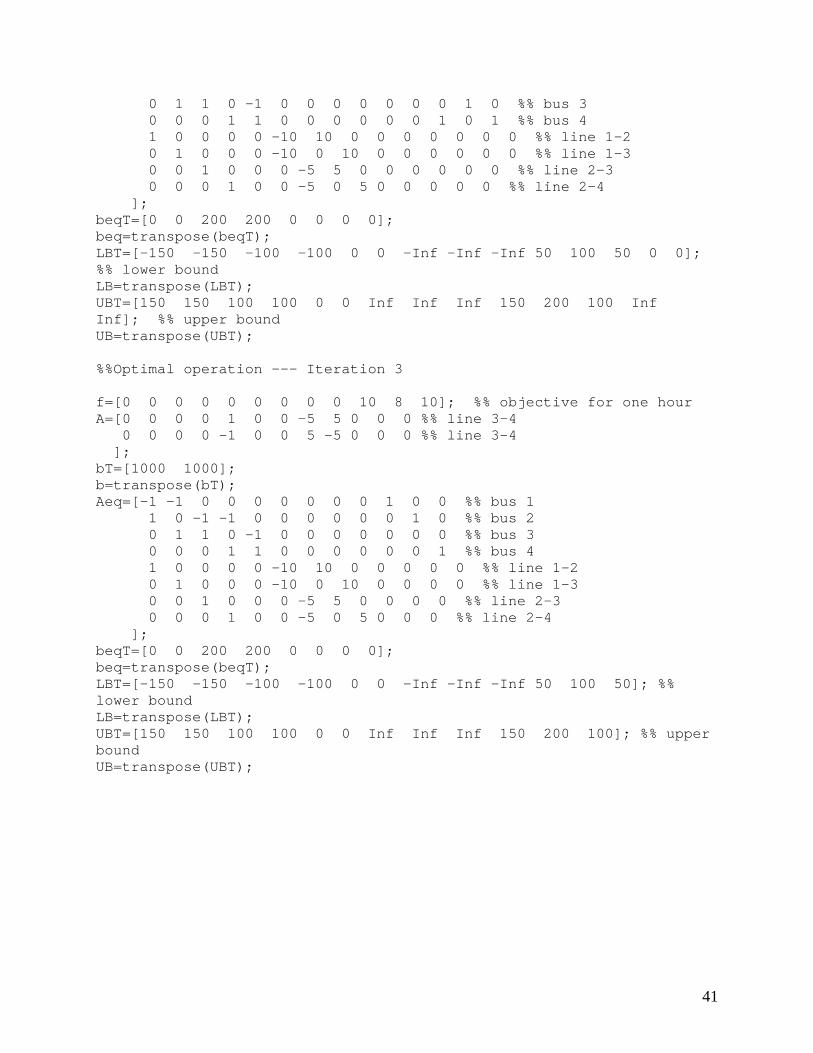
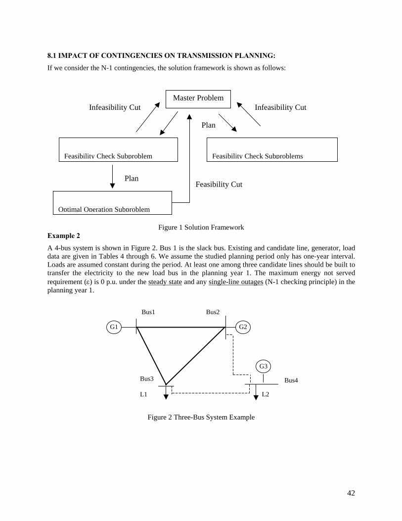
8. TRANSMISSION PLANNING The objective function of the transmission planning is to minimize the investment and operation cost under steady state while satisfying the system reliability requirement for each scenario ϕ. The objective function is formulated as follows:
( )[ ] ∑=
∑=
∑=
∑=
∑=
− ∗+−=T
t
B
b
NG
iibtGibtbt
T
t
CL
jtjjtjt POCDTXXCIYMin
1 1 1,
1 1)1( ** (8.1)
where i Unit index j Candidate line index b Load block index t Planning year index B Number of load blocks CL Number of candidate lines T Planning horizon NG Number of committed units CIjt Capital investment for candidate line j in year t DTbt Duration of load block b in year t OCibt Operating cost unit i among committed units at load block b in year t Xjt State variable associated with candidate line j in year t; 1: selected, 0: rejected.
( ). )( )1( itti XX ≤− 0Xi0 =PG,ibt Dispatched capacity of committed unit i at load block b in year t The first terms in the objective function (8.1) is the construction cost for new transmission lines. The second item is the operation cost. The set of planning constraints included in the transmission planning problem are: Constraints (8.2)-(8.5) represent the availability of capital investment funds in year t, projected line capacity for year t, maximum number of lines to be added at a planning year, and projected construction time, respectively.
),,2,1()(*1
)1( TtCIXXCI tCL
jtjjtjt L=≤−∑
=− (8.2)
),,2,1()(*1
)1( TtUCXXCap t
CL
jtjjtj L=≤−∑
=− (8.3)
),,2,1()(1
)1( TtUNXX t
CL
jtjjt L=≤−∑
=− (8.4)
),,2,1(),,2,1(0 TtNLjCTtifX jjt LL ==<= (8.5)
where Capj Capacity of line j CIt Capital investment in year t CTj Required construction time for candidate line j UCt Upper limit for line capacity added in year t UNt Upper limit for the # of lines added in year t
28
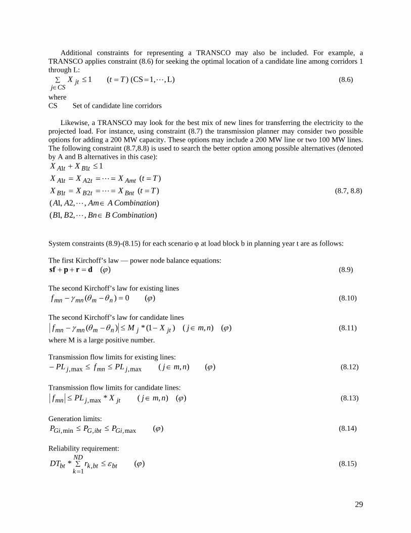
Additional constraints for representing a TRANSCO may also be included. For example, a TRANSCO applies constraint (8.6) for seeking the optimal location of a candidate line among corridors 1 through L:
L),1, (CS)(1 L==≤∑∈
TtXCSj
jt (8.6)
where CS Set of candidate line corridors Likewise, a TRANSCO may look for the best mix of new lines for transferring the electricity to the projected load. For instance, using constraint (8.7) the transmission planner may consider two possible options for adding a 200 MW capacity. These options may include a 200 MW line or two 100 MW lines. The following constraint (8.7,8.8) is used to search the better option among possible alternatives (denoted by A and B alternatives in this case):
),,2,1(),,2,1()()(
1
21
21
11
nCombinatioBBnBBnCombinatioAAmAATtXXXTtXXX
XX
BnttBtB
AmttAtA
tBtA
∈∈
========
≤+
L
L
L
L
(8.7, 8.8)
System constraints (8.9)-(8.15) for each scenario ϕ at load block b in planning year t are as follows: The first Kirchoff’s law — power node balance equations:
)(ϕdrpsf =++ (8.9) The second Kirchoff’s law for existing lines
)(0)( ϕθθγ =−− nmmnmnf (8.10) The second Kirchoff’s law for candidate lines
)(),()1(*)( ϕθθγ nmjXMf jtjnmmnmn ∈−≤−− (8.11)
where M is a large positive number. Transmission flow limits for existing lines:
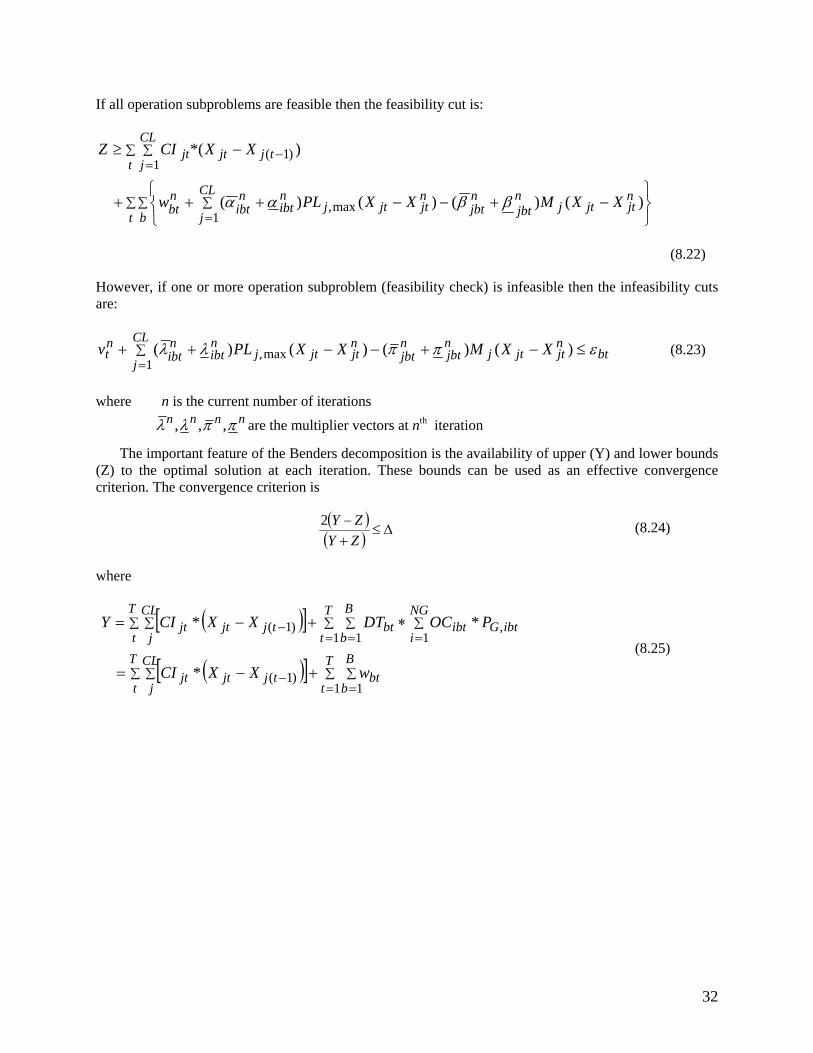
where k Load point index m,n Bus index ND Number of load points PGi,min Lower limit of generation of unit i PGi,max Upper limit of generation of unit i PLmn,max Capacity of line from node m to node n rk Curtailment of load k fmn Flow on line j from node m to node n γmn Line susceptance in vector form εbt Acceptable level of curtailment at load block b in year t ϕ Index of scenario (including the steady state and contingencies) d Node load in vector form f Power flow in vector form p Bus real generation in vector form r Curtailment in vector form s Node-branch incidence matrix The Benders decomposition is used here in which the problem is decomposed into a master problem and two subproblems representing feasibility and optimal operation subproblems. The master, which is a mixed integer program (MIP), considers an investment plan for transmission lines based on the available types of lines, suitable investment programs, and prospective locations based on the availability of corridor, and so on. Once the candidate lines are identified by the master problem, the feasibility subproblem will check whether this plan can meet system constraints (8.9)-(8.15). If the curtailment violations persist, the subproblem will form the corresponding Benders cut, which will be added to the master problem for solving the next iteration of the planning problem. Once the violations are removed, the solution of the optimal operation subproblem will measure the change in the total cost resulting from marginal changes in the proposed transmission planning. The iterative solution will form one or more constraints for the next iteration of the optimal operation subproblem by using dual multipliers. The iterative process will continue until a converged optimal solution is found.
Solution Procedure
The initial transmission planning master problem is formulated as follow:
( )[ ]∑ ∑ −−≥T
t
CL
jtjjtjt XXCIZ
ZMin
)1(* (8.16)
Subject to constraints (8.2)-(8.8).
The initial plan must satisfy the reliability requirement (8.15) for each scenario ϕ at load block b in planning year t to provide a secure supply while minimizing the cost of operation. The nth operation subproblem is feasible if and only if the optimal value of the following feasibility check subproblem is less than ε
(8.17) )(*1
, ϕ∑=
=ND
kbtkbt
nt rDTvMin
The objective (8.17) is to mitigate network violations and minimize the load curtailment by applying a generation redispatch. In this subproblem, constraints (8.9-8.14) are taken into account. Note that the constraints (8.11) and (8.13) corresponding to candidate lines can be rewritten as
30
πϕθθγ
πϕθθγ
)(),()1(*))((
)(),()1(*)(
nmjXMf
nmjXMf
jtjnmmnmn
jtjnmmnmn
∈−≤−−−
∈−≤−−
λϕ
λϕ
)(),(*
)(),(*
max,
max,
nmjXPLf
nmjXPLf
jtjmn
jtjmn
∈≤−
∈≤
If constraint (8.15) is not satisfied, the corresponding infeasibility cut given by (8.18) will be generated as follows:
btCL
j
njtjtj
njbt
njbt
njtjtj
nibt
nibt
nt XXMXXPLv εππλλ ≤−+−−++ ∑
=1max, )()()()( (8.18)
These n = 1,2,3,…,N-1 Benders cuts from the previous iterations are added to the master problem of transmission planning to get the nth trial investment plan. The process will be repeated until a feasible plan is found for meeting the requirement (8.15) on system reliability. If the above subproblem is feasible, then the optimal operation subproblem under the steady state for every year and load block is formulated as follows:
(8.19) ∑∗==
NG
iibtGibtbt
nbt POCDTwMin
1,*
Subject to the constraints (8.9)-(8.14). Note that the constraints (8.11) and (8.13) can be rewritten as
βθθγ
βθθγ
),()1(*))((
),()1(*)(
nmjXMf
nmjXMf
jtjnmmnmn
jtjnmmnmn
∈−≤−−−
∈−≤−−
α
α
),(*
),(*
max,
max,
nmjXPLf
nmjXPLf
jtjmn
jtjmn
∈≤−
∈≤
Therefore, the feasibility cut associated with the nth trial solution is
∑ ∑ ∑=
∑ ∑=
−
⎭⎬⎫
⎩⎨⎧
−+−−+++
−≥
t b
CL
j
njtjtj
njbt
njbt
njtjtj
nibt
nibt
nbt
t
CL
jtjjtjt
XXMXXPLw
XXCIZ
1max,
1)1(
)()()()(
)*(
ββαα
(8.20) Thus, the revised transmission planning problem MP1 (8.21) minimizes cost subject to planning constraints as well as feasibility and infeasibility cuts from the operation subproblems.
([∑ ∑ −−≥T
t
CL
jtjjtjt XXCIZ )]
ZMin
)1(* (8.21)
S.t. Planning constraints (8.2)-(8.7).
Feasibility and infeasibility cuts from previous iterations are:
31
If all operation subproblems are feasible then the feasibility cut is:
∑ ∑ ∑=
∑ ∑=
−
⎭⎬⎫
⎩⎨⎧
−+−−+++
−≥
t b
CL
j
njtjtj
njbt
njbt
njtjtj
nibt
nibt
nbt
t
CL
jtjjtjt
XXMXXPLw
XXCIZ
1max,
1)1(
)()()()(
)*(
ββαα
(8.22)
However, if one or more operation subproblem (feasibility check) is infeasible then the infeasibility cuts are:
btCL
j
njtjtj
njbt
njbt
njtjtj
nibt
nibt
nt XXMXXPLv εππλλ ≤−+−−++ ∑
=1max, )()()()( (8.23)
where n is the current number of iterations
nnnn ππλλ ,,, are the multiplier vectors at nth iteration
The important feature of the Benders decomposition is the availability of upper (Y) and lower bounds (Z) to the optimal solution at each iteration. These bounds can be used as an effective convergence criterion. The convergence criterion is
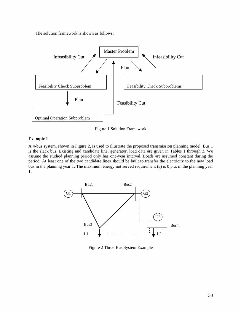
A 4-bus system, shown in Figure 2, is used to illustrate the proposed transmission planning model. Bus 1 is the slack bus. Existing and candidate line, generator, load data are given in Tables 1 through 3. We assume the studied planning period only has one-year interval. Loads are assumed constant during the period. At least one of the two candidate lines should be built to transfer the electricity to the new load bus in the planning year 1. The maximum energy not served requirement (ε) is 0 p.u. in the planning year 1.
Bus1
G2
Bus2
L2
Bus4
G3
Bus3
L1
G1
Figure 2 Three-Bus System Example
33
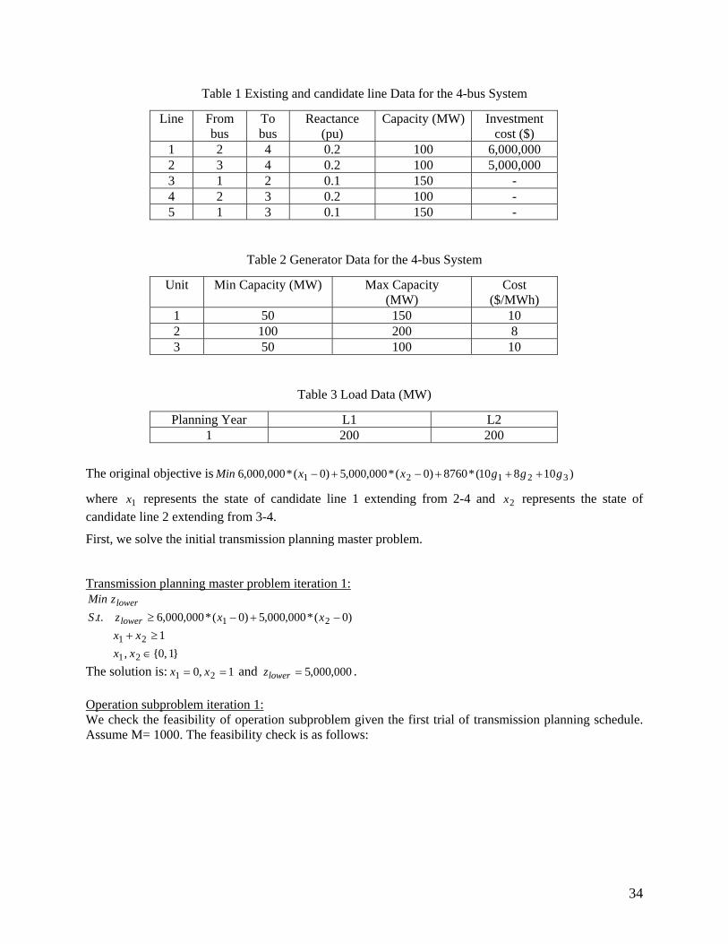
Table 1 Existing and candidate line Data for the 4-bus System
The original objective is )10810(*8760)0(*000,000,5)0(*000,000,6 32121 gggxxMin +++−+−
where represents the state of candidate line 1 extending from 2-4 and represents the state of candidate line 2 extending from 3-4.
1x 2x
First, we solve the initial transmission planning master problem.
Transmission planning master problem iteration 1:
}1,0{,1
)0(*000,000,5)0(*000,000,6..
21
21
21
∈≥+
−+−≥
xxxx
xxztSzMin
lower
lower
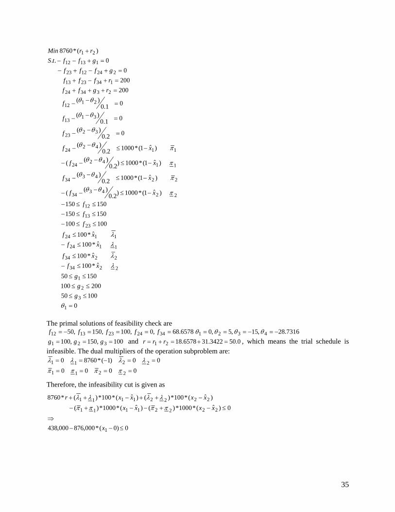
The solution is: and 1,0 21 == xx 000,000,5=lowerz . Operation subproblem iteration 1: We check the feasibility of operation subproblem given the first trial of transmission planning schedule. Assume M= 1000. The feasibility check is as follows:
34
224334
224334
114224
114224
3223
3113
2112
233424
1342313
2241223
11312
21
)ˆ1(*1000)2.0)((
)ˆ1(*10002.0)(
)ˆ1(*1000)2.0)((
)ˆ1(*10002.0)(
02.0)(
01.0)(
01.0)(
200200
00..
)(*8760
πθθ
πθθ
πθθ
πθθ
θθ
θθ
θθ
xf
xf
xf
xf
f
f
f
rgffrfffgfff
gfftSrrMin
−≤−−−
−≤−−
−≤−−−
−≤−−
=−−
=−−
=−−
=+++=+−+
=+−+−=+−−
+
010050
20010015050
ˆ*100ˆ*100
ˆ*100ˆ*100
100100150150150150
1
3
2
1
2234
2234
1124
1124
23
13
12
=≤≤≤≤
≤≤
≤−
≤
≤−≤
≤≤−≤≤−≤≤−
θ
λλ
λλ
gg
gxf
xf
xfxf
fff
The primal solutions of feasibility check are
6578.68,0,100,150,50 3424231312 ====−= fffff 7316.28,15,5,0 4321 −=−=== θθθθ 100,150,100 321 === ggg and 0.503422.316578.1821 =+=+= rrr , which means the trial schedule is
infeasible. The dual multipliers of the operation subproblem are:
000000)1(*87600
2211
2211
====
==−==
ππππλλλλ
Therefore, the infeasibility cut is given as
0)0(*000,876000,438
0)ˆ(*1000*)()ˆ(*1000*)()ˆ(*100*)()ˆ(*100*)(*8760
1
22221111
22221111
≤−−⇒
≤−+−−+−
−++−++
x
xxxxxxxxr
ππππλλλλ
35
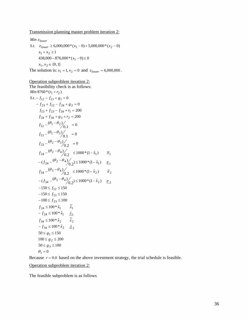
Transmission planning master problem iteration 2:
}1,0{,0)0(*000,876000,438
1)0(*000,000,5)0(*000,000,6..
21
1
21
21
∈≤−−
≥+−+−≥
xxx
xxxxztS
zMin
lower
lower
The solution is: and 0,1 21 == xx 000,000,6=lowerz . Operation subproblem iteration 2: The feasibility check is as follows:
224334
224334
114224
114224
3223
3113
2112
233424
1342313
2241223
11312
21
)ˆ1(*1000)2.0)((
)ˆ1(*10002.0)(
)ˆ1(*1000)2.0)((
)ˆ1(*10002.0)(
02.0)(
01.0)(
01.0)(
200200
00..
)(*8760
πθθ
πθθ
πθθ
πθθ
θθ
θθ
θθ
xf
xf
xf
xf
f
f
f
rgffrfffgfff
gfftSrrMin
−≤−−−
−≤−−
−≤−−−
−≤−−
=−−
=−−
=−−
=+++=+−+
=+−+−=+−−
+
100100150150150150
23
13
12
≤≤−≤≤−≤≤−
fff
010050
20010015050
ˆ*100ˆ*100
ˆ*100ˆ*100
1
3
2
1
2234
2234
1124
1124
=≤≤≤≤
≤≤
≤−
≤
≤−≤
θ
λλ
λλ
gg
gxf
xf
xfxf
Because based on the above investment strategy, the trial schedule is feasible. 0.0=r
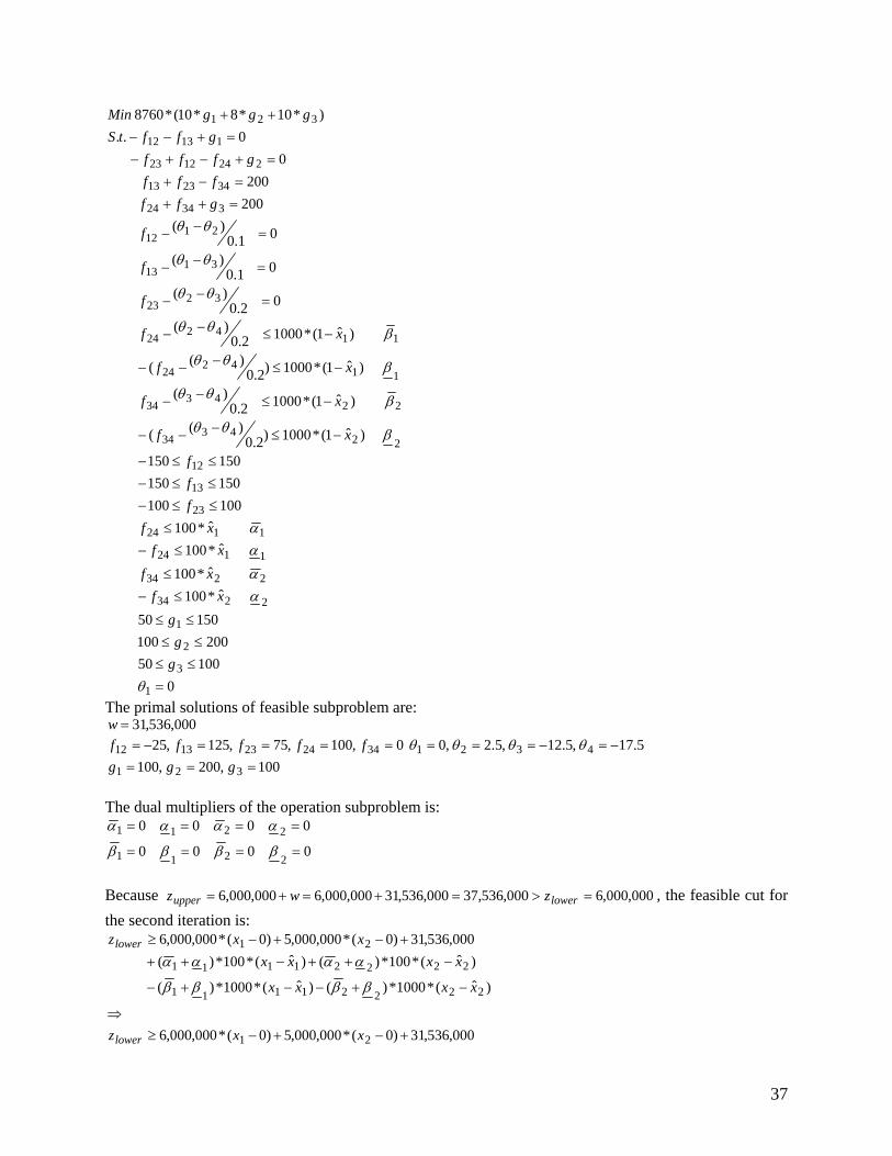
Operation subproblem iteration 2: The feasible subproblem is as follows
36
02.0)(
01.0)(
01.0)(
200200
00..
)*10*8*10(*8760
3223
3113
2112
33424
342313
2241223
11312
321
=−−
=−−
=−−
=++=−+
=+−+−=+−−
++
θθ
θθ
θθ
f
f
f
gfffff
gfffgfftS
gggMin
010050
20010015050
ˆ*100ˆ*100
ˆ*100ˆ*100
100100150150150150
)ˆ1(*1000)2.0)((
)ˆ1(*10002.0)(
)ˆ1(*1000)2.0)((
)ˆ1(*10002.0)(
1
3
2
1
2234
2234
1124
1124
23
13
12
224334
224334
114224
114224
=≤≤≤≤
≤≤
≤−
≤
≤−≤
≤≤−≤≤−≤≤−
−≤−−−
−≤−−
−≤−−−
−≤−−
θ
αααα
βθθ
βθθ
βθθ
βθθ
gg
gxf
xfxf
xffff
xf
xf
xf
xf
The primal solutions of feasible subproblem are: 000,536,31=w
The solution is: and 0,1 21 == xx 000,536,37=lowerz . Operation subproblem iteration 3: Because of based on the above investment strategy, the trial schedule is feasible. 0.0=r
Operation subproblem iteration 3: According to calculations, the primal solution of feasible subproblem is:
Because , the optimal solution is obtained, which show that selecting the line 2-4 can satisfy the system curtailment requirement, though it has a higher investment cost than the candidate line 3-4.
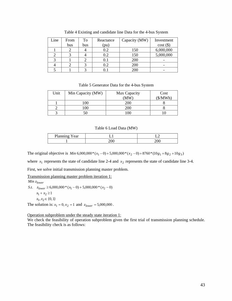
A 4-bus system is shown in Figure 2. Bus 1 is the slack bus. Existing and candidate line, generator, load data are given in Tables 4 through 6. We assume the studied planning period only has one-year interval. Loads are assumed constant during the period. At least one among three candidate lines should be built to transfer the electricity to the new load bus in the planning year 1. The maximum energy not served requirement (ε) is 0 p.u. under the steady state and any single-line outages (N-1 checking principle) in the planning year 1.
Bus1
G2
Bus2
L2
Bus4
G3
Bus3
L1
G1
Figure 2 Three-Bus System Example
42
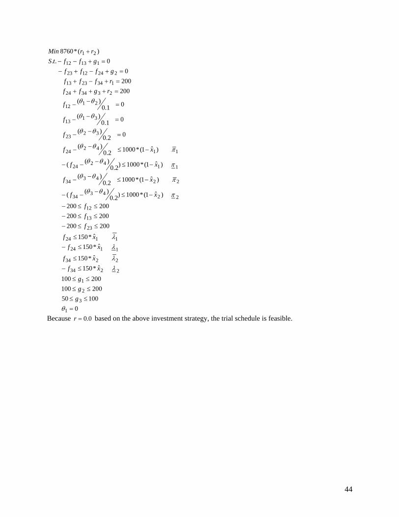
Table 4 Existing and candidate line Data for the 4-bus System
The original objective is )10810(*8760)0(*000,000,5)0(*000,000,6 32121 gggxxMin +++−+−
where represents the state of candidate line 2-4 and represents the state of candidate line 3-4. 1x 2x
First, we solve initial transmission planning master problem.
Transmission planning master problem iteration 1:
}1,0{,1
)0(*000,000,5)0(*000,000,6..
21
21
21
∈≥+
−+−≥
xxxx
xxztSzMin
lower
lower
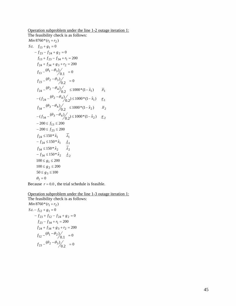
The solution is: and 1,0 21 == xx 000,000,5=lowerz . Operation subproblem under the steady state iteration 1: We check the feasibility of operation subproblem given the first trial of transmission planning schedule. The feasibility check is as follows:
43
224334
224334
114224
114224
3223
3113
2112
233424
1342313
2241223
11312
21
)ˆ1(*1000)2.0)((
)ˆ1(*10002.0)(
)ˆ1(*1000)2.0)((
)ˆ1(*10002.0)(
02.0)(
01.0)(
01.0)(
200200
00..
)(*8760
πθθ
πθθ
πθθ
πθθ
θθ
θθ
θθ
xf
xf
xf
xf
f
f
f
rgffrfffgfff
gfftSrrMin
−≤−−−
−≤−−
−≤−−−
−≤−−
=−−
=−−
=−−
=+++=+−+
=+−+−=+−−
+
010050
200100200100
ˆ*150ˆ*150
ˆ*150ˆ*150
200200200200200200
1
3
2
1
2234
2234
1124
1124
23
13
12
=≤≤≤≤≤≤
≤−
≤
≤−≤
≤≤−≤≤−≤≤−
θ
λλ
λλ
ggg
xfxf
xfxf
fff
Because based on the above investment strategy, the trial schedule is feasible. 0.0=r
44
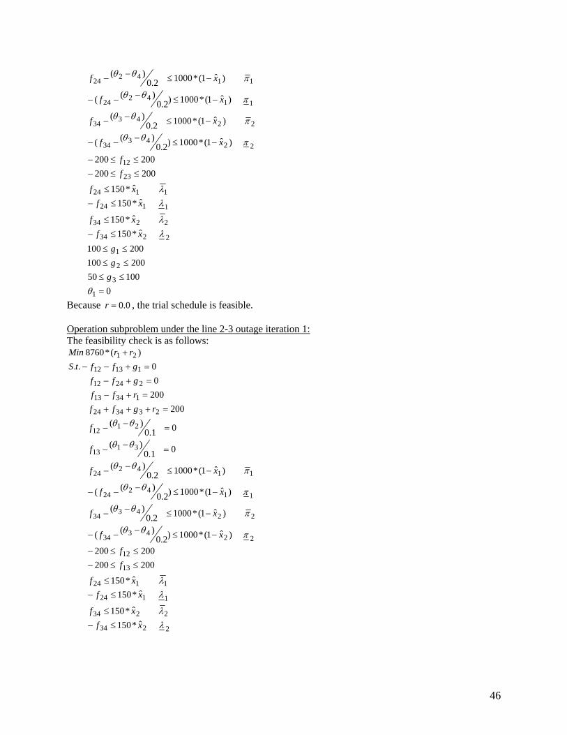
Operation subproblem under the line 1-2 outage iteration 1: The feasibility check is as follows:
224334
224334
114224
114224
3223
3113
233424
1342313
22423
113
21
)ˆ1(*1000)2.0)((
)ˆ1(*10002.0)(
)ˆ1(*1000)2.0)((
)ˆ1(*10002.0)(
02.0)(
01.0)(
200200
00..
)(*8760
πθθ
πθθ
πθθ
πθθ
θθ
θθ
xf
xf
xf
xf
f
f
rgffrfff
gffgftS
rrMin
−≤−−−
−≤−−
−≤−−−
−≤−−
=−−
=−−
=+++=+−+
=+−−=++
010050
200100200100
ˆ*150ˆ*150
ˆ*150ˆ*150
200200200200
1
3
2
1
2234
2234
1124
1124
23
13
=≤≤≤≤≤≤
≤−
≤
≤−≤
≤≤−≤≤−
θ
λλ
λλ
ggg
xfxf
xfxf
ff
Because , the trial schedule is feasible. 0.0=r Operation subproblem under the line 1-3 outage iteration 1: The feasibility check is as follows:
02.0)(
01.0)(
200200
00..
)(*8760
3223
2112
233424
13423
2241223
112
21
=−−
=−−
=+++=+−
=+−+−=+−+
θθ
θθ
f
f
rgffrff
gfffgftS
rrMin
45
224334
224334
114224
114224
)ˆ1(*1000)2.0)((
)ˆ1(*10002.0)(
)ˆ1(*1000)2.0)((
)ˆ1(*10002.0)(
πθθ
πθθ
πθθ
πθθ
xf
xf
xf
xf
−≤−−−
−≤−−
−≤−−−
−≤−−
010050
200100200100
ˆ*150ˆ*150
ˆ*150ˆ*150
200200200200
1
3
2
1
2234
2234
1124
1124
23
12
=≤≤≤≤≤≤
≤−
≤
≤−≤
≤≤−≤≤−
θ
λλ
λλ
ggg
xfxf
xfxf
ff
Because , the trial schedule is feasible. 0.0=r Operation subproblem under the line 2-3 outage iteration 1: The feasibility check is as follows:
224334
224334
114224
114224
3113
2112
233424
13413
22412
11312
21
)ˆ1(*1000)2.0)((
)ˆ1(*10002.0)(
)ˆ1(*1000)2.0)((
)ˆ1(*10002.0)(
01.0)(
01.0)(
20020000..
)(*8760
πθθ
πθθ
πθθ
πθθ
θθ
θθ
xf
xf
xf
xf
f
f
rgffrffgffgfftS
rrMin
−≤−−−
−≤−−
−≤−−−
−≤−−
=−−
=−−
=+++=+−=+−=+−−
+
2234
2234
1124
1124
13
12
ˆ*150ˆ*150
ˆ*150ˆ*150
200200200200
λλ
λλ
xfxf
xfxf
ff
≤−≤
≤−≤
≤≤−≤≤−
46
010050
200100200100
1
3
2
1
=≤≤≤≤≤≤
θggg
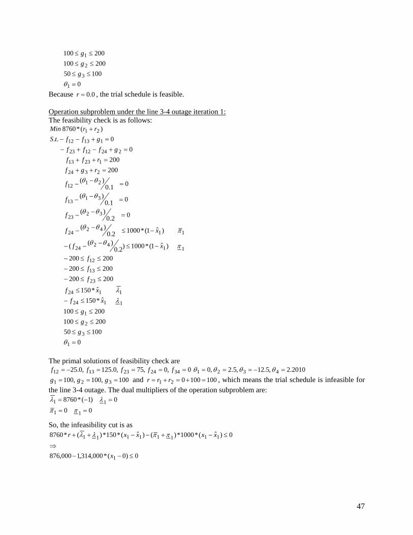
Because , the trial schedule is feasible. 0.0=r Operation subproblem under the line 3-4 outage iteration 1: The feasibility check is as follows:
114224
114224
3223
3113
2112
2324
12313
2241223
11312
21
)ˆ1(*1000)2.0)((
)ˆ1(*10002.0)(
02.0)(
01.0)(
01.0)(
200200
00..
)(*8760
πθθ
πθθ
θθ
θθ
θθ
xf
xf
f
f
f
rgfrff
gfffgfftS
rrMin
−≤−−−
−≤−−
=−−
=−−
=−−
=++=++
=+−+−=+−−
+
010050
200100200100
ˆ*150ˆ*150
200200200200200200
1
3
2
1
1124
1124
23
13
12
=≤≤≤≤≤≤
≤−≤
≤≤−≤≤−≤≤−
θ
λλ
ggg
xfxf
fff
The primal solutions of feasibility check are
0,0,75,0.125,0.25 3424231312 ====−= fffff 2010.2,5.12,5.2,0 4321 =−=== θθθθ 100,100,100 321 === ggg and 100100021 =+=+= rrr , which means the trial schedule is infeasible for
the line 3-4 outage. The dual multipliers of the operation subproblem are:
000)1(*8760
11
11
==
=−=
ππλλ
So, the infeasibility cut is as
0)0(*000,314,1000,876
0)ˆ(*1000*)()ˆ(*150*)(*8760
1
11111111
≤−−⇒
≤−+−−++
x
xxxxr ππλλ
47
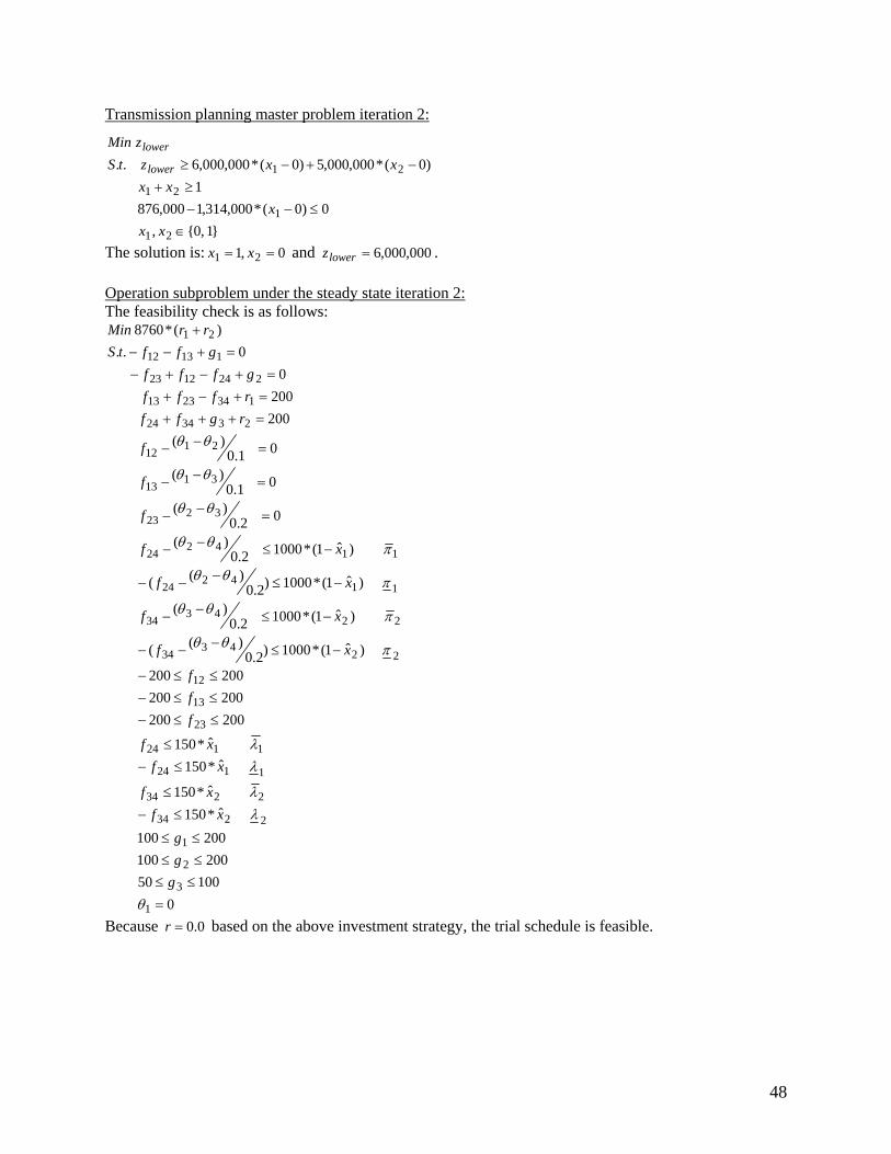
Transmission planning master problem iteration 2:
}1,0{,0)0(*000,314,1000,876
1)0(*000,000,5)0(*000,000,6..
21
1
21
21
∈≤−−
≥+−+−≥
xxx
xxxxztS
zMin
lower
lower
The solution is: and 0,1 21 == xx 000,000,6=lowerz . Operation subproblem under the steady state iteration 2: The feasibility check is as follows:
224334
224334
114224
114224
3223
3113
2112
233424
1342313
2241223
11312
21
)ˆ1(*1000)2.0)((
)ˆ1(*10002.0)(
)ˆ1(*1000)2.0)((
)ˆ1(*10002.0)(
02.0)(
01.0)(
01.0)(
200200
00..
)(*8760
πθθ
πθθ
πθθ
πθθ
θθ
θθ
θθ
xf
xf
xf
xf
f
f
f
rgffrfffgfff
gfftSrrMin
−≤−−−
−≤−−
−≤−−−
−≤−−
=−−
=−−
=−−
=+++=+−+
=+−+−=+−−
+
010050
200100200100
ˆ*150ˆ*150
ˆ*150ˆ*150
200200200200200200
1
3
2
1
2234
2234
1124
1124
23
13
12
=≤≤≤≤≤≤
≤−
≤
≤−≤
≤≤−≤≤−≤≤−
θ
λλ
λλ
ggg
xfxf
xfxf
fff
Because based on the above investment strategy, the trial schedule is feasible. 0.0=r
48
Operation subproblem under the line 1-2 outage iteration 2: The feasibility check is as follows:
224334
224334
114224
114224
3223
3113
233424
1342313
22423
113
21
)ˆ1(*1000)2.0)((
)ˆ1(*10002.0)(
)ˆ1(*1000)2.0)((
)ˆ1(*10002.0)(
02.0)(
01.0)(
200200
00..
)(*8760
πθθ
πθθ
πθθ
πθθ
θθ
θθ
xf
xf
xf
xf
f
f
rgffrfff
gffgftS
rrMin
−≤−−−
−≤−−
−≤−−−
−≤−−
=−−
=−−
=+++=+−+
=+−−=++
010050
200100200100
ˆ*150ˆ*150
ˆ*150ˆ*150
200200200200
1
3
2
1
2234
2234
1124
1124
23
13
=≤≤≤≤≤≤
≤−
≤
≤−≤
≤≤−≤≤−
θ
λλ
λλ
ggg
xfxf
xfxf
ff
Because , the trial schedule is feasible. 0.0=r
49
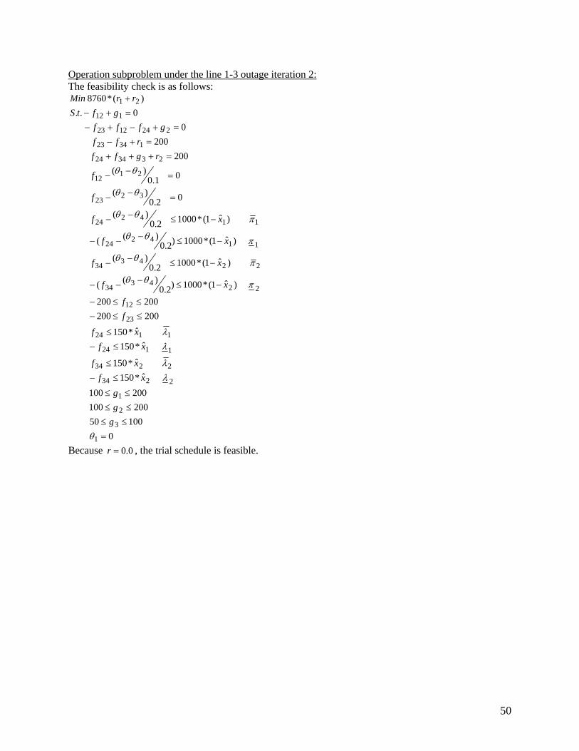
Operation subproblem under the line 1-3 outage iteration 2: The feasibility check is as follows:
224334
224334
114224
114224
3223
2112
233424
13423
2241223
112
21
)ˆ1(*1000)2.0)((
)ˆ1(*10002.0)(
)ˆ1(*1000)2.0)((
)ˆ1(*10002.0)(
02.0)(
01.0)(
200200
00..
)(*8760
πθθ
πθθ
πθθ
πθθ
θθ
θθ
xf
xf
xf
xf
f
f
rgffrff
gfffgftS
rrMin
−≤−−−
−≤−−
−≤−−−
−≤−−
=−−
=−−
=+++=+−
=+−+−=+−+
010050
200100200100
ˆ*150ˆ*150
ˆ*150ˆ*150
200200200200
1
3
2
1
2234
2234
1124
1124
23
12
=≤≤≤≤≤≤
≤−
≤
≤−≤
≤≤−≤≤−
θ
λλ
λλ
ggg
xfxf
xfxf
ff
Because , the trial schedule is feasible. 0.0=r
50
Operation subproblem under the line 2-3 outage iteration 2: The feasibility check is as follows:
224334
224334
114224
114224
3113
2112
233424
13413
22412
11312
21
)ˆ1(*1000)2.0)((
)ˆ1(*10002.0)(
)ˆ1(*1000)2.0)((
)ˆ1(*10002.0)(
01.0)(
01.0)(
20020000..
)(*8760
πθθ
πθθ
πθθ
πθθ
θθ
θθ
xf
xf
xf
xf
f
f
rgffrffgffgfftS
rrMin
−≤−−−
−≤−−
−≤−−−
−≤−−
=−−
=−−
=+++=+−=+−=+−−
+
010050
200100200100
ˆ*150ˆ*150
ˆ*150ˆ*150
200200200200
1
3
2
1
2234
2234
1124
1124
13
12
=≤≤≤≤≤≤
≤−
≤
≤−≤
≤≤−≤≤−
θ
λλ
λλ
ggg
xfxf
xfxf
ff
Because , the trial schedule is feasible. 0.0=r
51
Operation subproblem under the line 2-4 outage iteration 2: The feasibility check is as follows:
224334
224334
3223
3113
2112
2334
1342313
21223
11312
21
)ˆ1(*1000)2.0)((
)ˆ1(*10002.0)(
02.0)(
01.0)(
01.0)(
200200
00..
)(*8760
πθθ
πθθ
θθ
θθ
θθ
xf
xf
f
f
f
rgfrfff
gffgfftS
rrMin
−≤−−−
−≤−−
=−−
=−−
=−−
=++=+−+
=++−=+−−
+
010050
200100200100
ˆ*150ˆ*150
200200200200200200
1
3
2
1
2234
2234
23
13
12
=≤≤≤≤≤≤
≤−
≤
≤≤−≤≤−≤≤−
θ
λλ
ggg
xfxf
fff
The primal solutions of feasibility check are
0,0,75,0.125,0.25 3424231312 ====−= fffff 3346.12,5.12,5.2,0 4321 −=−=== θθθθ 100,100,100 321 === ggg and 100100021 =+=+= rrr , which means the trial schedule is infeasible for
the line 2-4 outage. The dual multipliers of the operation subproblem are:
000)1(*8760
22
22
==
=−=
ππλλ
Therefore, the infeasibility cut is as
0)0(*000,314,1000,876
0)ˆ(*1000*)()ˆ(*150*)(*8760
2
22222222
≤−−⇒
≤−+−−++
x
xxxxr ππλλ
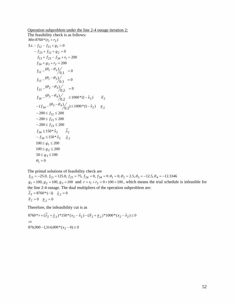
52
Transmission planning master problem iteration 3:
}1,0{,0)0(*000,314,1000,8760)0(*000,314,1000,876
1)0(*000,000,5)0(*000,000,6..
21
2
1
21
21
∈≤−−≤−−
≥+−+−≥
xxxx
xxxxztS
zMin
lower
lower
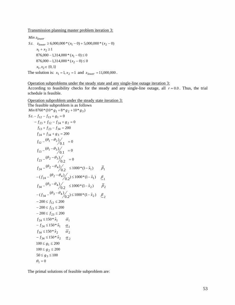
The solution is: and 1,1 21 == xx 000,000,11=lowerz . Operation subproblems under the steady state and any single-line outage iteration 3: According to feasibility checks for the steady and any single-line outage, all . Thus, the trial schedule is feasible.
0.0=r
Operation subproblem under the steady state iteration 3: The feasible subproblem is as follows
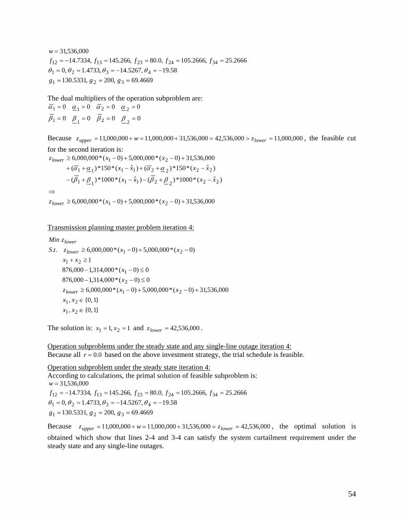
The solution is: and 1,1 21 == xx 000,536,42=lowerz . Operation subproblems under the steady state and any single-line outage iteration 4: Because all based on the above investment strategy, the trial schedule is feasible. 0.0=r
Operation subproblem under the steady state iteration 4: According to calculations, the primal solution of feasible subproblem is:
Because , the optimal solution is obtained which show that lines 2-4 and 3-4 can satisfy the system curtailment requirement under the steady state and any single-line outages.