Benefits of Overall Equipment Effectiveness (OEE) Techniques in Metal Mining Environments Executive summary Within the metals and mining industry trends such as volatility and increasing operating costs are forcing stakeholders to seek new low-cost ways to increase productivity. Increasing asset performance has now become a high priority. However, the overall complexity of the process sometimes masks those areas where productivity benefits can be derived. This paper identifies the largest opportunities for improvements in asset performance within the metals and mining industry. by Yong The and Stewart Johnston
Transcript
Benefits of Overall Equipment Effectiveness (OEE) Techniques in Metal Mining Environments
Executive summary
Within the metals and mining industry trends such as
volatility and increasing operating costs are forcing
stakeholders to seek new low-cost ways to increase
productivity. Increasing asset performance has
now become a high priority. However, the overall
complexity of the process sometimes masks those
areas where productivity benefits can be derived.
This paper identifies the largest opportunities for
improvements in asset performance within the metals
and mining industry.
by Yong The and Stewart Johnston
Schneider Electric White Paper 2
Benefits of Overall Equipment Effectiveness (OEE) Techniques in Metal Mining Environments
Introduction
OEE in metalliferous operations
Metalliferous processes are complex from a control and physical extraction and delivery perspective. Raw material predictability, feed material sizing and chemical reaction processes relies on a multitude of heavy industrial equipment across multiple staged sub-processes in order to liberate metallic materials away from the waste. Metallurgists have to balance feed properties, consumable use and operating rate (of equipment) in order to achieve the highest productivity within a profitable range – or find the “sweet spot” in operating conditions. Addressing this balance requires a combination of experienced personnel, advanced real-time control, and operational intelligence systems.
This paper analyses how operational intelligence can be used to validate data derived from the control systems and operator input in order to render operations more predictable and productive. The concept of OEE (Overall Equipment Effectiveness), which was first popularized during the 1980’s and 1990’s, is discussed in conjunction with “lean manufacturing” theories in order to streamline an entire process.
In an ideal world all assets should be performing in a sustainable manner at its designed capacity. The key issue for operations is to understand how much their asset can be pushed before it becomes unsustainable. Given the complexity of metalliferous operations, there will always be unplanned downtime and performance losses. However, by observing historical data of maximum sustainable production KPI’s it is possible to use that as a benchmark for the performance of the asset. Once this mark has been exceeded on as consistent basis, then a new benchmark should then be used as the target for future OEE calculations. This fosters a culture of continuous improvement. Real-time OEE can be expressed in the following formula:
Real-time OEE = Current Actual Production ÷ Maximum Sustainable Rate (of Production)
OEE serves as a benchmark for how efficiently the assets of the company are being used. It is the ratio of product that has been produced to the amount of product that could have been produced, given ideal conditions in the processing plant.
The maximum sustainable production is a reasonable expectation of what the plant should be able to achieve under optimal conditions. This will be defined below as Maximum Sustainable Rate (MSR) of production. OEE is a convenient dimensionless number which can be used to measure plant performance in a uniform manner allowing plant management to drive positive behaviour and provide motivation for plant improvements.
The components of OEE need to be related to one another in order to allow for proper measurement. Since an easily comparable factor is time, use is made of the Time Usage Model (see adjoining text box) in order to divide overall calendar time into meaningful components. This allows for substandard behaviour classification and eases the identification of the root causes of low OEE.
● The types of operational production losses include the following:
● Loss due to lack of demand for products
● Loss due to availability of equipment
● Loss due to slow or sub-optimal performance of process or equipment,
● Loss due to production of poor quality or recovery of product.
The scope of OEE includes all areas within the metal mining plant that contribute to all or any of the above components with the exception of the demand component which is market driven.
OEE is used as a continuous improvement tool, and it is often focused on areas of the operations that have been cited as bottlenecks. However the quality can be measured in various locations but usually the prime location is that which is producing the end product.
Maximum sustainable rate and continuous improvement
In the course of an OEE project, the term “sustainable” has to be defined and remain consistent in relation to the different KPI’s to be measured. “Sustainable” should be defined as a period of time that is sufficiently long but, should be time that passes without process degradation or equipment breakdown. Reviewing historical process data over a period of a year or more should unveil what the maximum sustainable rate should be for all required KPI’s. Given ideal circumstances, the plant should operate at this maximum sustainable rate throughout the scheduled production period. This would constitute an OEE of 100%.
As the performance of the operation improves and shows that it can achieve and sustain rates above the previously established Maximum Sustainable Rate (MSR) then the MSR needs to be adjusted to show the
Time Usage
ModelA TUM defines how a calendar
time period is broken down
in components and sub-
components of productive
and unproductive time
categories. This allows metrics
to be evaluated for availability,
utilization and delays.
The Time Usage Model is
generally defined by the
operations (production &
maintenance teams) to match
their process and the types of
equipment within that process.
Schneider Electric White Paper 3
Benefits of Overall Equipment Effectiveness (OEE) Techniques in Metal Mining Environments
Time: A common unit of measure
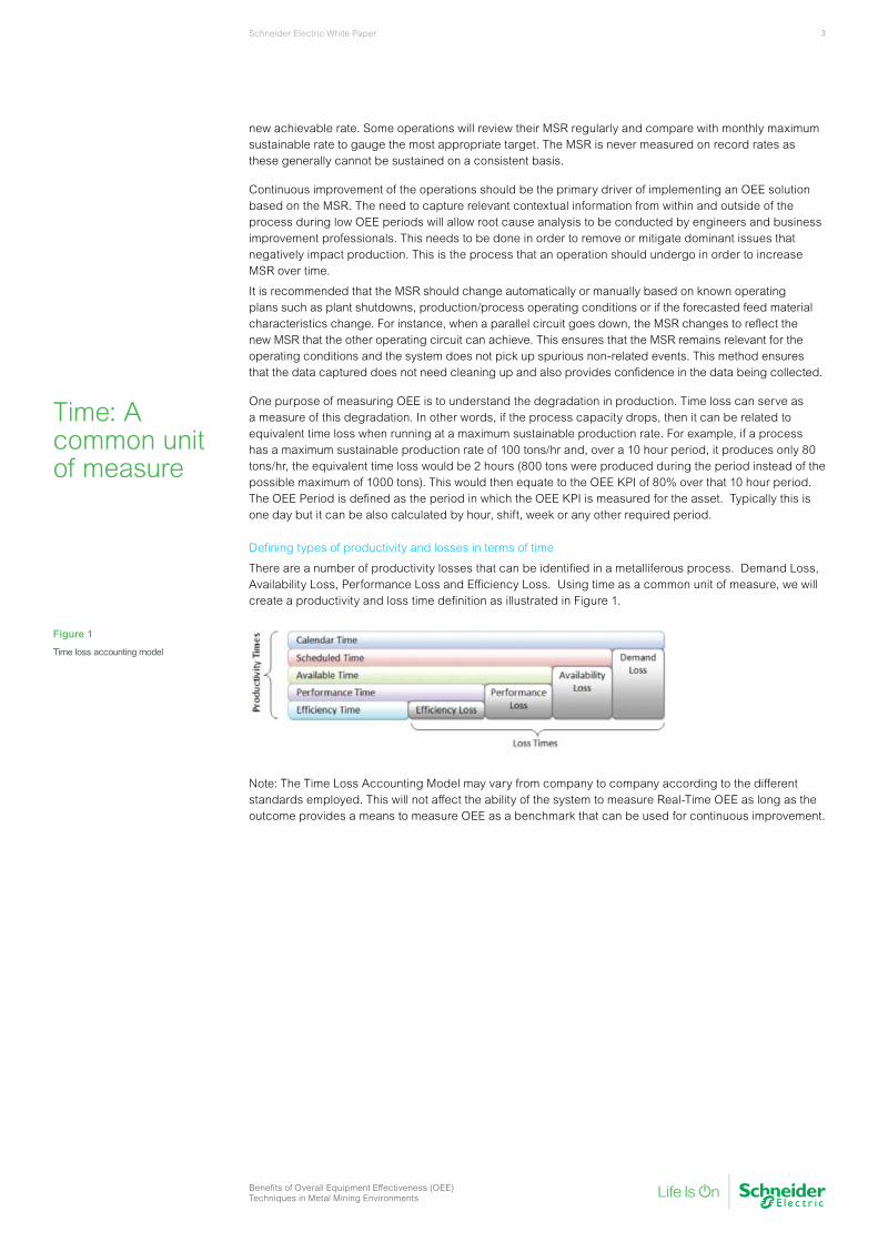
Figure 1
Time loss accounting model
new achievable rate. Some operations will review their MSR regularly and compare with monthly maximum sustainable rate to gauge the most appropriate target. The MSR is never measured on record rates as these generally cannot be sustained on a consistent basis.
Continuous improvement of the operations should be the primary driver of implementing an OEE solution based on the MSR. The need to capture relevant contextual information from within and outside of the process during low OEE periods will allow root cause analysis to be conducted by engineers and business improvement professionals. This needs to be done in order to remove or mitigate dominant issues that negatively impact production. This is the process that an operation should undergo in order to increase MSR over time.
It is recommended that the MSR should change automatically or manually based on known operating plans such as plant shutdowns, production/process operating conditions or if the forecasted feed material characteristics change. For instance, when a parallel circuit goes down, the MSR changes to reflect the new MSR that the other operating circuit can achieve. This ensures that the MSR remains relevant for the operating conditions and the system does not pick up spurious non-related events. This method ensures that the data captured does not need cleaning up and also provides confidence in the data being collected.
One purpose of measuring OEE is to understand the degradation in production. Time loss can serve as a measure of this degradation. In other words, if the process capacity drops, then it can be related to equivalent time loss when running at a maximum sustainable production rate. For example, if a process has a maximum sustainable production rate of 100 tons/hr and, over a 10 hour period, it produces only 80 tons/hr, the equivalent time loss would be 2 hours (800 tons were produced during the period instead of the possible maximum of 1000 tons). This would then equate to the OEE KPI of 80% over that 10 hour period. The OEE Period is defined as the period in which the OEE KPI is measured for the asset. Typically this is one day but it can be also calculated by hour, shift, week or any other required period.
Defining types of productivity and losses in terms of time
There are a number of productivity losses that can be identified in a metalliferous process. Demand Loss, Availability Loss, Performance Loss and Efficiency Loss. Using time as a common unit of measure, we will create a productivity and loss time definition as illustrated in Figure 1.
Note: The Time Loss Accounting Model may vary from company to company according to the different standards employed. This will not affect the ability of the system to measure Real-Time OEE as long as the outcome provides a means to measure OEE as a benchmark that can be used for continuous improvement.
Schneider Electric White Paper 4
Benefits of Overall Equipment Effectiveness (OEE) Techniques in Metal Mining Environments
OEE calculated using time measure
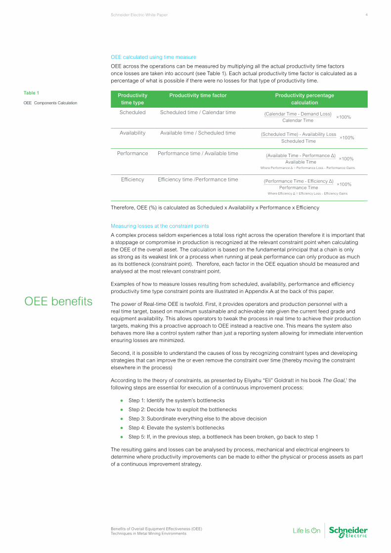
OEE across the operations can be measured by multiplying all the actual productivity time factors once losses are taken into account (see Table 1). Each actual productivity time factor is calculated as a percentage of what is possible if there were no losses for that type of productivity time.
Productivity time type
Productivity time factor Productivity percentage calculation
Scheduled Scheduled time / Calendar time
Availability Available time / Scheduled time
Performance Performance time / Available time
Efficiency Efficiency time /Performance time
Therefore, OEE (%) is calculated as Scheduled x Availability x Performance x Efficiency
Measuring losses at the constraint points
A complex process seldom experiences a total loss right across the operation therefore it is important that a stoppage or compromise in production is recognized at the relevant constraint point when calculating the OEE of the overall asset. The calculation is based on the fundamental principal that a chain is only as strong as its weakest link or a process when running at peak performance can only produce as much as its bottleneck (constraint point). Therefore, each factor in the OEE equation should be measured and analysed at the most relevant constraint point.
Examples of how to measure losses resulting from scheduled, availability, performance and efficiency productivity time type constraint points are illustrated in Appendix A at the back of this paper.
The power of Real-time OEE is twofold. First, it provides operators and production personnel with a real time target, based on maximum sustainable and achievable rate given the current feed grade and equipment availability. This allows operators to tweak the process in real time to achieve their production targets, making this a proactive approach to OEE instead a reactive one. This means the system also behaves more like a control system rather than just a reporting system allowing for immediate intervention ensuring losses are minimized.
Second, it is possible to understand the causes of loss by recognizing constraint types and developing strategies that can improve the or even remove the constraint over time (thereby moving the constraint elsewhere in the process)
According to the theory of constraints, as presented by Eliyahu “Eli” Goldratt in his book The Goal,1 the following steps are essential for execution of a continuous improvement process:
● Step 1: Identify the system’s bottlenecks
● Step 2: Decide how to exploit the bottlenecks
● Step 3: Subordinate everything else to the above decision
● Step 4: Elevate the system’s bottlenecks
● Step 5: If, in the previous step, a bottleneck has been broken, go back to step 1
The resulting gains and losses can be analysed by process, mechanical and electrical engineers to determine where productivity improvements can be made to either the physical or process assets as part of a continuous improvement strategy.
Table 1
OEE Components Calculation
OEE benefits
×100%Calendar Time
(Calendar Time - Demand Loss)
×100%Scheduled Time
(Scheduled Time) - Availability Loss
×100%Available Time
(Available Time - Performance Δ)
Where Performance Δ = Performance Loss – Performance Gains
×100%Performance Time
(Performance Time - Efficiency Δ)
Where Efficiency Δ = Efficiency Loss – Efficiency Gains
Schneider Electric White Paper 5
Benefits of Overall Equipment Effectiveness (OEE) Techniques in Metal Mining Environments
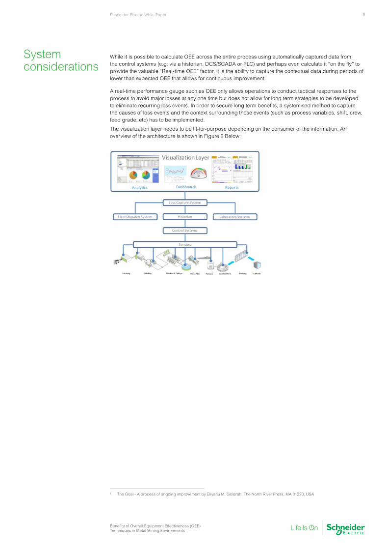
While it is possible to calculate OEE across the entire process using automatically captured data from the control systems (e.g. via a historian, DCS/SCADA or PLC) and perhaps even calculate it “on the fly” to provide the valuable “Real-time OEE” factor, it is the ability to capture the contextual data during periods of lower than expected OEE that allows for continuous improvement.
A real-time performance gauge such as OEE only allows operations to conduct tactical responses to the process to avoid major losses at any one time but does not allow for long term strategies to be developed to eliminate recurring loss events. In order to secure long term benefits, a systemised method to capture the causes of loss events and the context surrounding those events (such as process variables, shift, crew, feed grade, etc) has to be implemented.
The visualization layer needs to be fit-for-purpose depending on the consumer of the information. An overview of the architecture is shown in Figure 2 Below:
System considerations
1 The Goal - A process of ongoing improvement by Eliyahu M. Goldratt, The North River Press, MA 01230, USA
Schneider Electric White Paper 6
Benefits of Overall Equipment Effectiveness (OEE) Techniques in Metal Mining Environments
An Australian Mining Company was one of the first businesses to implement this new OEE approach. By deploying solid change management practices and role based training, technology adoption and an OEE reporting system were made possible.
Reports were distributed on a daily basis to operations, supervisors and management. Process engineers, maintenance and asset managers were able to drill down into the data to determine the root cause of the problems. This allowed operational teams to provide management with root cause analysis and corrective action plans.
Specific examples of the changes resulting in the implementation of the OEE system include:
● Operators can execute on operations targets in a proactive manner, in near real time reducing time and production losses.
● Operators understood how to avoid the natural inclination to push the process harder since such excessive demand leads to process disruption and loss of production. Therefore, operators changed the way they approached plant production problems and were not pushed by management to drive production beyond realistic capacities.
● The management team based the Maximum Sustainable Rate (MSR) on metal tonnes rather than total tonnage. This provided a better understanding of how pushing tonnes has an impact on materials grade losses and on metal recovery.
● A more harmonious, collaborative approach to fixing problems has been established because the various teams now share a common understanding of process constraints and efficiency gains.
● New technology tools provided the functionality to enable users to clearly define the root causes to focus on the big ticket items that gave them biggest return on their time and investment.
● Clarity was provided on how to achieve optimum productivity which, in turn, has driven improvement to assets, resources, and processes.
In the clients words
“We should see improvements from the OEE initiative in excess of $1 Billion in our first year”
Metals and mining operations wishing to initiate a migration to a realtime OEE approach should consider the following short and long term steps:
Within the next few weeks:
Begin to plan a roadmap. Assess which areas of the mining operation infrastructure represent the biggest pain points.
Within the next 6 months:
Leverage technology. Identify an initial project with low up-front investment that can result in positive results over a relatively short period of time (like an immediate opportunity to reduce extraction waste). This approach will build confidence and support for future OEE related projects.
Within the next year:
Think of ways to integrate operational silos and generate funding. Drive collaboration with partners who can provide tools for rapid implementation and who have the technical expertise and global presence to support long term infrastructure integration projects.
Case study
Conclusion
Schneider Electric White Paper 7
Benefits of Overall Equipment Effectiveness (OEE) Techniques in Metal Mining Environments
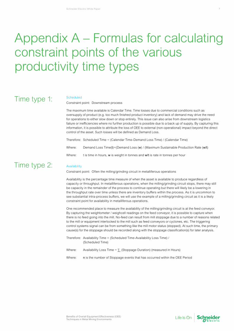
Scheduled
Constraint point: Downstream process
The maximum time available is Calendar Time. Time losses due to commercial conditions such as oversupply of product (e.g. too much finished product inventory) and lack of demand may drive the need for operations to either slow down or stop entirely. This issue can also arise from downstream logistics failure or inefficiencies where no further production is possible due to a back up of supply. By capturing this information, it is possible to attribute the loss of OEE to external (non-operational) impact beyond the direct control of the asset. Such losses will be defined as Demand Loss.
Therefore: Scheduled Time = (Calendar Time-Demand Loss Time) / (Calendar Time)
Where: Demand Loss Time(t)=(Demand Loss (w) / (Maximum Sustainable Production Rate (w/t)
Where: t is time in hours, w is weight in tonnes and w/t is rate in tonnes per hour
Availability
Constraint point: Often the milling/grinding circuit in metalliferous operations
Availability is the percentage time measure of when the asset is available to produce regardless of capacity or throughput. In metalliferous operations, when the milling/grinding circuit stops, there may still be capacity in the remainder of the process to continue operating but there will likely be a lowering in the throughput rate over time unless there are inventory buffers within the process. As it is uncommon to see substantial intra-process buffers, we will use the example of a milling/grinding circuit as it is a likely constraint point for availability in metalliferous operations.
One recommended place to measure the availability of the milling/grinding circuit is at the feed conveyor. By capturing the weightometer / weighcell readings on the feed conveyor, it is possible to capture when there is no feed going into the mill. No-feed can result from mill stoppage due to a number of reasons related to the mill or equipment interlocked to the mill such as feed conveyors or cyclones, etc. The triggering control systems signal can be from something like the mill motor status (stopped). At such time, the primary cause(s) for the stoppage should be recorded along with the stoppage classification(s) for later analysis.
Therefore: Availability Time = (Scheduled Time-Availability Loss Time) / (Scheduled Time)
Where: Availability Loss Time = ∑n (Stoppage Duration) (measured in Hours)
Where: n is the number of Stoppage events that has occurred within the OEE Period
Time type 1:
Time type 2:
Appendix A – Formulas for calculating constraint points of the various productivity time types
Schneider Electric White Paper 8
Benefits of Overall Equipment Effectiveness (OEE) Techniques in Metal Mining Environments
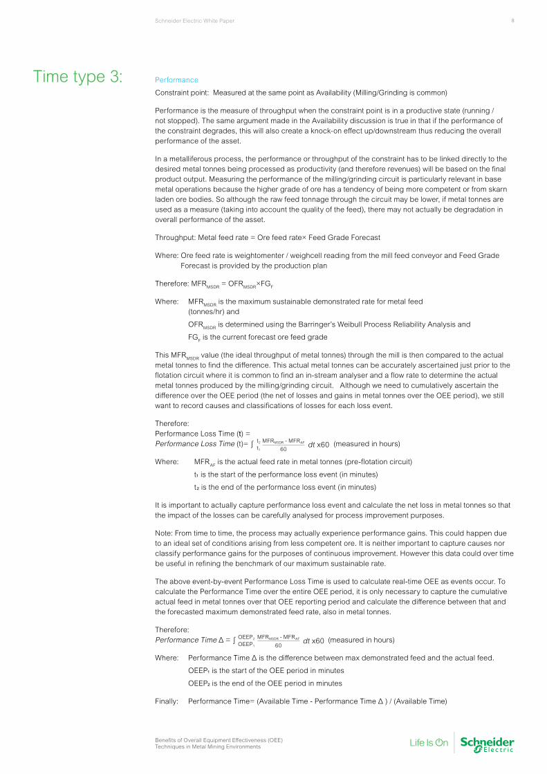
Performance
Constraint point: Measured at the same point as Availability (Milling/Grinding is common)
Performance is the measure of throughput when the constraint point is in a productive state (running / not stopped). The same argument made in the Availability discussion is true in that if the performance of the constraint degrades, this will also create a knock-on effect up/downstream thus reducing the overall performance of the asset.
In a metalliferous process, the performance or throughput of the constraint has to be linked directly to the desired metal tonnes being processed as productivity (and therefore revenues) will be based on the final product output. Measuring the performance of the milling/grinding circuit is particularly relevant in base metal operations because the higher grade of ore has a tendency of being more competent or from skarn laden ore bodies. So although the raw feed tonnage through the circuit may be lower, if metal tonnes are used as a measure (taking into account the quality of the feed), there may not actually be degradation in overall performance of the asset.
Where: Ore feed rate is weightomenter / weighcell reading from the mill feed conveyor and Feed Grade Forecast is provided by the production plan
Therefore: MFRMSDR = OFRMSDR×FGF
Where: MFRMSDR is the maximum sustainable demonstrated rate for metal feed (tonnes/hr) and
OFRMSDR is determined using the Barringer’s Weibull Process Reliability Analysis and
FGF is the current forecast ore feed grade
This MFRMSDR value (the ideal throughput of metal tonnes) through the mill is then compared to the actual metal tonnes to find the difference. This actual metal tonnes can be accurately ascertained just prior to the flotation circuit where it is common to find an in-stream analyser and a flow rate to determine the actual metal tonnes produced by the milling/grinding circuit. Although we need to cumulatively ascertain the difference over the OEE period (the net of losses and gains in metal tonnes over the OEE period), we still want to record causes and classifications of losses for each loss event.
Therefore: Performance Loss Time (t) = Performance Loss Time (t)= ∫ (measured in hours)
Where: MFRAF is the actual feed rate in metal tonnes (pre-flotation circuit)
t1 is the start of the performance loss event (in minutes)
t2 is the end of the performance loss event (in minutes)
It is important to actually capture performance loss event and calculate the net loss in metal tonnes so that the impact of the losses can be carefully analysed for process improvement purposes.
Note: From time to time, the process may actually experience performance gains. This could happen due to an ideal set of conditions arising from less competent ore. It is neither important to capture causes nor classify performance gains for the purposes of continuous improvement. However this data could over time be useful in refining the benchmark of our maximum sustainable rate.
The above event-by-event Performance Loss Time is used to calculate real-time OEE as events occur. To calculate the Performance Time over the entire OEE period, it is only necessary to capture the cumulative actual feed in metal tonnes over that OEE reporting period and calculate the difference between that and the forecasted maximum demonstrated feed rate, also in metal tonnes.
Therefore: Performance Time Δ = ∫ (measured in hours)
Where: Performance Time Δ is the difference between max demonstrated feed and the actual feed.
OEEP1 is the start of the OEE period in minutes
OEEP2 is the end of the OEE period in minutes
Finally: Performance Time= (Available Time - Performance Time Δ ) / (Available Time)
Time type 3:
t2
t1
MFRMSDR - MFRAF
60dt x60
OEEP2
OEEP1
MFRMSDR - MFRAF
60dt x60
Schneider Electric White Paper 9
Benefits of Overall Equipment Effectiveness (OEE) Techniques in Metal Mining Environments
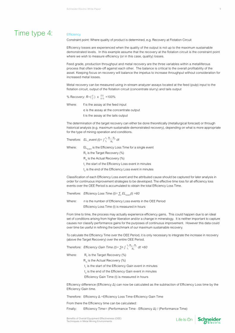
Efficiency
Constraint point: Where quality of product is determined, e.g. Recovery at Flotation Circuit
Efficiency losses are experienced when the quality of the output is not up to the maximum sustainable demonstrated levels. In this example assume that the recovery at the flotation circuit is the constraint point where we wish to measure efficiency (or in this case, quality) losses.
Feed grade, production throughput and metal recovery are the three variables within a metalliferous process that often trade-off against each other. The balance is critical to the overall profitability of the asset. Keeping focus on recovery will balance the impetus to increase throughput without consideration for increased metal losses.
Metal recovery can be measured using in-stream analyzer assays located at the feed (pulp) input to the flotation circuit, output of the flotation circuit (concentrate slurry) and tails output
% Recovery: R=( ) x ×100%
Where: f is the assay at the feed input
c is the assay at the concentrate output
t is the assay at the tails output
The determination of the target recovery can either be done theoretically (metallurgical forecast) or through historical analysis (e.g. maximum sustainable demonstrated recovery), depending on what is more appropriate for the type of mining operation and conditions.
Therefore: EL_event (t)= ∫
Where: ELevent is the Efficiency Loss Time for a single event
RT is the Target Recovery (%)
RA is the Actual Recovery (%)
t1 the start of the Efficiency Loss event in minutes
t2 is the end of the Efficiency Loss event in minutes
Classification of each Efficiency Loss event and the attributed cause should be captured for later analysis in order for continuous improvement strategies to be developed. The effective time loss for all efficiency loss events over the OEE Period is accumulated to obtain the total Efficiency Loss Time.
Therefore: Efficiency Loss Time (t)= ∑n ELevent(t) ×60
Where: n is the number of Efficiency Loss events in the OEE Period
Efficiency Loss Time (t) is measured in hours
From time to time, the process may actually experience efficiency gains. This could happen due to an ideal set of conditions arising from higher liberation and/or a change in mineralogy. It is neither important to capture causes nor classify performance gains for the purposes of continuous improvement. However this data could over time be useful in refining the benchmark of our maximum sustainable recovery.
To calculate the Efficiency Time over the OEE Period, it is only necessary to integrate the increase in recovery (above the Target Recovery) over the entire OEE Period.
Therefore: Efficiency Gain Time (t)= ∑n ∫ dt ×60
Where: RT is the Target Recovery (%)
RA is the Actual Recovery (%)
t1 is the start of the Efficiency Gain event in minutes
t2 is the end of the Efficiency Gain event in minutes
Efficiency Gain Time (t) is measured in hours
Efficiency difference (Efficiency Δ) can now be calculated as the subtraction of Efficiency Loss time by the Efficiency Gain time.
Therefore: Efficiency Δ =Efficiency Loss Time-Efficiency Gain Time
In capturing the OEE loss events as described above, it is possible to create a Pareto of causes, (Pareto principle: A few contributors are responsible for the bulk of the effects–the 80/20 rule) classifications, and loss-causing equipments/processes (amongst other contextual information) that has resulted in the greatest impact to the operation from a financial/cost perspective. This will help in continuous improvement effort by bringing focus and direction.
The way to benchmark the success of such improvement initiatives will be through the use of the OEE KPI, or the OEE factor (%).
OEE=Scheduled Time × Available Time ×Performance Time × Efficiency Time ×100%
The OEE KPI
About the authorsYong The is the Global Strategic Alliance Manager for Schneider Electric’s Industry Business and has been in the forefront of Schneider Electric’s MES offering to the Mining, Metals and Mineral Processing industry since 2006. A graduate of University of California, Berkeley in Robotics and Automation, he has over 30 years experience in control systems, software engineering, enterprise software implementations and strategic consulting as applied to a variety of industries including mining, telecommunications and utilities. Yong’s background in mechanical engineering, electrical engineering, and business consulting has helped him in developing innovative solutions for global Schneider Electric customers.
Stewart Johnston is Schneider Electrics Enterprise Solutions Manager for lifecycle management of Ampla, Wonderware MES, Supply Chain Optimisation (SCO) and Intelligence EMI. He is uniquely experienced with knowledge to design and implement fully Integrated ERP/MES and Control solutions for mining, resource and manufacturing operations and how to use those systems to optimise and improve the production and supply chain processes.
Stewart has a Diploma of Metallurgy and IT qualifications on Network and Web Design along with over 15 years in designing and implementing Manufacturing Execution Systems to meet customer business needs. He has over 20 years relevant industrial experience, working in different mining, resource and manufacturing operations including, gold, nickel, copper, fertilizer and LNG operations.