Bericht des Instituts f ¨ ur Aerodynamik und Str ¨ omungstechnik Report of the Institute of Aerodynamics and Flow Technology IB 124-2007/3 A Fourth Order Semi-Implicit Runge-Kutta Method for the Compressible Euler Equations Ursula Mayer, Richard P. Dwight Herausgeber: Deutsches Zentrum f ¨ ur Luft- und Raumfahrt e.V. Institut f ¨ ur Aerodynamik und Str ¨ omungstechnik Lilienthalplatz 7, 38108 Braunschweig ISSN 1614-7790 Stufe der Zug ¨ anglichkeit: 1 Braunschweig, im April 2007 Institutsdirektor: Prof. Dr.-Ing. habil. C.-C. Rossow Verfasser: Ursula Mayer Richard P. Dwight Abteilung: Numerical Methods Abteilungsleiter: Prof. Dr.-Ing. N. Kroll Der Bericht enth ¨ alt: 24 Seiten 10 Bilder 0 Tabellen 15 Literaturstellen
Transcript
Bericht des Instituts fur Aerodynamik und Stromungstechnik
Report of the Institute of Aerodynamics and Flow Technology
IB 124-2007/3
A Fourth Order Semi-Implicit Runge-Kutta Method for the
Compressible Euler Equations
Ursula Mayer, Richard P. Dwight
Herausgeber:
Deutsches Zentrum fur Luft- und Raumfahrt e.V.
Institut fur Aerodynamik und Stromungstechnik
Lilienthalplatz 7, 38108 Braunschweig
ISSN 1614-7790
Stufe der Zuganglichkeit: 1
Braunschweig, im April 2007
Institutsdirektor:
Prof. Dr.-Ing. habil. C.-C. Rossow
Verfasser:
Ursula Mayer
Richard P. Dwight
Abteilung: Numerical Methods
Abteilungsleiter:
Prof. Dr.-Ing. N. Kroll
Der Bericht enthalt:
24 Seiten
10 Bilder
0 Tabellen
15 Literaturstellen
Abstract
Efficient time integration is of the utmost concern for unsteady flow computations. Withinthis context two semi-implicit Runge-Kutta methods of 3rd- and 4th-order and their applica-tion to two-dimensional compressible inviscid flows are presented. The semi-implicit methodsdeveloped here are expected to be considerably more stable than fully explicit methods, andmore efficient than fully implicit methods. This is achieved by constructing an explicit 3rd-order Runge-Kutta method with the property that an arbitrary stabilizing implicit term may beadded at each stage without degrading the order of convergence. This feature allows one toapply implicit operators based on approximate Jacobians, the choice of operator being madeonly with regard to stability, efficiency and storage requirements. A corresponding 4th-ordermethod is obtained by linear Richardson extrapolation on the original 3rd order scheme, andboth schemes are supplied with a local error estimation and time-step control. Numerical ex-amples are performed on various cases using the DLR TAU-Code, a finite volume RANS solver,with a Lower-Upper Symmetric Gauss-Seidel implicit operator. It demonstrated that bothsemi-implicit schemes are significantly more stable than the corresponding explicit schemes,and in addition they are able to outperform standard fully implicit methods by up to a factorof 10 in terms of CPU time for given accuracy.
5 Numerical Examples 135.1 An Expansion Fan in a Shock tube on a Structured Grid . . . . . . . . . . . . . . . 13
5.2 Euler Flow over a Forward Facing Step on a Rectangular Grid . . . . . . . . . . . 16
5.3 Euler Flow over a Ramp on a Triangular Grid . . . . . . . . . . . . . . . . . . . . . 18
6 Conclusions 22
ii
1 Introduction
The level of detail and complexity demanded of numerical simulation is increasing continu-ously in many engineering fields. In computational aerodynamics time-accurate flow compu-tations are becoming increasingly important and relevant to industry, but require dispropor-tionate computing resources in comparison to stationary problems.
Efficiency improvements of flow solvers in aerodynamics have concentrated principally onthe rapid solution of steady flows using such techniques as Full Approximation Storage (FAS)multigrid and approximate (and inexact) Newton solvers. As a result the application of thesealgorithms has become refined and well understood. When unsteady simulations are required,they are typically performed using a dual time algorithm [8], where an analogue of the non-linear steady problem is solved at each time-step using aforementioned steady solvers. Theresult is an order-of-magnitude higher cost for unsteady simulation, which has precluded itsapplication in many areas. New algorithms for the efficient solution of unsteady flows aretherefore of utmost concern.
The commonly used fully explicit and fully implicit time integration schemes each have a majordisadvantage: explicit schemes suffer from a restriction on the time-step size for stiff problems;implicit schemes in contrast are often unconditionally stable and the time-step may be cho-sen based only on resolution of the physical processes of interest, but a nonlinear system ofequations must be solved at every integration step.
Any semi-implicit scheme might therefore be expected to combine the advantages of the twoapproaches. It should be considerably more stable than an explicit scheme, and significantlycheaper per time-step than an implicit scheme.
One candidate method is due to Nikitin [11], who applied his semi-implicit Runge-Kutta method(RK) to the incompressible Navier-Stokes equations for problems including flow in a drivencavity. The scheme is based on a three-stage third order explicit RK scheme, whose structure iscarefully chosen such that it is possible to add an arbitrary implicit term to each stage withoutcompromising the order of the method. This allows the choice of the implicit part based only onthe requirements of stability, time-accuracy being automatically satisfied. Therefore the highlytuned approximate Newton methods developed in the pursuit of efficient schemes for steadyproblems may be used as stabilization terms for unsteady problems.
This is in sharp contrast to such semi-implicit schemes as the second-order Adams-Bashforth-Crank-Nicolson (ABCN) method for the convection-diffusion equation, which treats the con-vective terms with Adams-Bashforth and the diffusive terms with Crank-Nicolson, and wherethe formulation and solution of the implicit part must be exact in order for the scheme to beof the desired order. Modern examples for the compressible Navier-Stokes equations are thethird-order semi-implicit RK methods of Yoh and Zhong [13], which also require exact treat-ment of the implicit part. This condition restricts the application of such methods to situationsin with the stiffness is confined to a few terms that may be additively separated from non-stiffterms, and whose exact implicit treatment is much cheaper than the exact implicit treatment of
1
Introduction 2
the entire system. For example Yoh and Zhong have applied their scheme to combustion prob-lems with only the strong source terms - which dominate the stability of the scheme - treatedimplicitly [14]. With the scheme of Nikitin it is possible to treat all terms implicitly at low costby using approximate implicit methods.
Since the term Semi-Implicit Runge-Kutta (SIRK) is already well-established for denoting schemesof the ABCN type, we will refer to the present class of methods as Unconstrained ImplicitRunge-Kutta (UIRK), in reference to the complete absence of constraints on the implicit opera-tor.
This report considers the third-order time-accurate, semi-implicit RK method of Nikitin appliedto the compressible Euler equations. A semi-implicit fourth-order method is constructed bylinear Richardson extrapolation on the original scheme, and for both schemes an embeddedlower-order method is used to provide local error estimation and time-step control.
The most crucial choice involved in the scheme - in terms of storage requirements, efficiency,and accuracy - is the choice of the implicit operator, its approximate flux Jacobian and the solverfor the resulting linear system. In this preliminary study we consider only application of ahighly optimized version of the Lower-Upper Symmetric Gauss-Seidel (LU-SGS) algorithm [15,5]. This involves a first-order approximation of the Jacobian, constructed on-the-fly, wherebyall terms in the spatial discretization, including boundary conditions, are present. One sweepof symmetric Gauss-Seidel is applied to give a very rough approximation to the solution ofthis linear system. The result is an implicit method that is unconditionally stable for inviscidproblems, while being cheaper per iteration than a three-stage RK scheme, as well as requiringless memory. This cheap unconditional stability makes LU-SGS an ideal scheme for the currentapplication.
The order of both semi-implicit Runge-Kutta methods is verified numerically for several testcases on various structured and unstructured grids. It is demonstrated that in several casesthe UIRK scheme outperforms dual time by a factor of 10 in terms of CPU time for a givenaccuracy. All implementations and tests are done within the finite volume RANS solver theDLR TAU-Code [6].
This report is organized as follows: the governing Euler equations and their unstructured finitevolume discretization are described in Sections 2.1 and 2.2 respectively, then the third-orderUIRK scheme and its fourth-order extrapolation are discussed in detail in Sections 3.1 and3.2. Stability of the schemes is examined in Section 3.3, and the time-step control algorithm isdeveloped in Section 3.4. Section 4 describes LU-SGS, and numerical tests are undertaken inSection 5.
124-2007/3
2 Spatial Discretization
2.1 The Euler Equations
The governing equations are the compressible Euler equations in two dimensions, which ex-pressed in conservative form are
∂W
∂t+
∂
∂xif c
i (W ) =∂W
∂t+ R(W ) = 0, (2.1)
where the summation convention is applied on the index i and the residual R(W ) denotes thesum of the convective flux derivatives.
The conservative state vector W is defined as
W =
ρρuρvρE
, (2.2)
where U = (u, v)T is the velocity vector and ρ is the density. The convective fluxes f ci in the
two coordinate directions i ∈ x, y are
f cx =
ρuρuu + pρuvρHu
, f cy =
ρvρvuρvv + pρHv
. (2.3)
The pressure p for a calorically perfect gas is defined by the state equation
p = (γ − 1)ρ E −1
2U2, (2.4)
where E is the specific total energy per unit mass and γ is the gas dependent ratio of specificheats, which is 1.4 for air. The total enthalpy H is given by
H = E +p
ρ. (2.5)
2.2 Finite Volume Discretization
In the theory of finite volumes the discretization is not applied to the differential form of theEuler equations (2.1), but to the integral form. The advantage in this approach lies in the factthat integral form allows easily ensuring conservation of mass, momentum and energy over anarbitrary control volume Ω. The integral form can be understood such that the rate of change
3
2. Spatial Discretization 4
of each of the conservative quantities, integrated over Ω, equals the flux of each through thewalls of Ω:
∂
∂t
∫
ΩW dΩ +
∮
∂Ωf c(W ) · nd(∂Ω) = 0. (2.6)
The boundary of Ω is denoted ∂Ω and n its outer normal. The problem domain is decomposedinto a grid of non-overlapping, cell-vertex median-dual control volumes that are approximateVoronoı volumes of a primary grid.
This semi-discretization in space leads to
∂
∂t
∫
Ωi
Wi dΩ = −R(Wi), (2.7)
where the residual R contains the full discretization of the integral over the convective fluxes.
Assuming that W varies linearly over the control volume Ω, we get
|Ωi|dWi
d t= −R(Wi), (2.8)
where |Ωi| is the volume of Ωi.
In the following we use both upwind and central convective fluxes depending on the problemat hand. The central flux is based on the Jameson-Schmitt-Turkel (JST) scheme [9], when up-wind is used it is the AUSM-DV scheme of Wada and Liou [12]. Despite the various residualflux discretizations, the Jacobian used in LU-SGS remains the same, based on a first-order Lax-Friedrichs flux. Investigations have demonstrated that the effect of reducing the flux used inthe Jacobian to first-order dominates the effect of any particular choice of flux function [5].
3.1 A Third-Order Semi-Implicit Runge-Kutta Scheme
In this section the semi-implicit third-order Runge-Kutta method (RK3 SI) developed by Nikitin [11],is described in relation to a general autonomous ordinary differential equation (2.8). This UIRKscheme is based on a particular third-order explicit Runge-Kutta scheme (RK3 EXP), where ineach stage an arbitrary implicit stabilization term is added, whose order is the same as the trun-cation error of the stage, and which may therefore also be regarded as a perturbation or errorterm.
The three stages of the explicit part are:
|Ω|W ′ − W n
∆t= −
2
3R(W n), (3.1)
|Ω|W ′′ − W n
∆t= −
1
3R(W n) −
1
3R(W ′), (3.2)
|Ω|W n+1 − W n
∆t= −
1
4R(W n) −
3
4R(W ′′). (3.3)
which is a special case of the one-parameter family of third-order three-stage schemes with RKcoefficient tableau
023
23
23
23 − 1
4b14b
14
34 − b b
with b = 3/4 [3]. For reasons that will become clear, the construction of the semi-implicitmethod relies upon two features of this scheme: that the abscissas of the second and thirdstages are identical, so that W ′ and W ′′ are evaluated at the same time increment t + 2
3∆t, andthat the term R(W ′) does not appear in the final quadrature for W n+1.
Observe that the following relations hold for the above scheme:
which we now perturb by adding an implicit term to each stage as follows:
|Ω|W ′ − W n
∆t= −
2
3R(W n) − γ L (W ′ − W n), (3.7)
|Ω|W ′′ − W n
∆t= −
1
3R(W n) −
1
3R(W ′) − γ L (W ′′ − W ′), (3.8)
|Ω|W n+1 − W n
∆t= −
1
4R(W n) −
3
4R(W ′′) − γ L (W n+1 − W n+1). (3.9)
Here the linear operator L is some approximation of the flux Jacobian ∂R/∂W , and γ is apositive coefficient that controls the relative strength of the implicit terms. The need for the - asyet undefined - intermediate solution W n+1 is explained later on.
First consider the right-hand side (RHS) of (3.7), which is obviously an O(∆t) perturbationof the RHS of (3.1), which results in an O(∆t2) variation in W ′ and R(W ′), i.e. the order ofaccuracy of these terms has not been reduced. Analogously the RHS of (3.8) is an O(∆t2)perturbation of the RHS of (3.2), resulting in an O(∆t3) variation in W ′′ and R(W ′′), and againthere is no reduction in accuracy. Note that this was only possible because W ′ and W ′′ wereevaluated at the same time increment, otherwise W ′′ − W ′ would have been O(∆t).
Finally, assuming that W n+1 = W (tn+1) + O(∆t3) the RHS of equation (3.9) is an O(∆t3)perturbation of the RHS of (3.3) causing an O(∆t4) variation in W n+1. Thus at each stageand overall the semi-implicit scheme retains its order of accuracy. In particular the local errorW n+1 − W (tn+1) is still O(∆t4), and the UIRK scheme is third-order.
It remains to define W n+1, a second-order accurate approximation to the solution at the fulltime increment, which may be written:
|Ω|W n+1 − W n
∆t= −
1
4R(W n) −
3
4R(W ′) − γ L (W n+1 − W n+1), (3.10)
where W n+1 is an O(∆t) approximation of W (tn+1), which is chosen as
W n+1 =3
2(αW ′ + (1 − α)W ′′) −
1
2W n, (3.11)
where the real parameter α can be chosen arbitrarily.
Of course although the formal order of the method is preserved, the addition of effectivelyarbitrary terms must negatively influence its absolute accuracy. It makes sense therefore tochoose as small a value for γ as possible, bearing in mind that the method is more implicit,and therefore more stable, for large values of γ. There is a compromise to be made for eachproblem, each time-step and each choice of L. For example, if the time-step is in a region forwhich the original explicit method is stable, then γ = 0 is very likely to be optimal, as the added“error” has been reduced as far as possible. Since the UIRK scheme is also about a factor of fourmore expensive than the baseline explicit scheme per time-step, it is therefore only attractivefor time-steps greater than four times the maximum stable explicit time-step.
In Section 3.3 it will be shown that for linear R, and L the exact Jacobian, the scheme is A-stable for γ ≥ 1
3 . But while it has been noted that LU-SGS is unconditionally stable for steadyproblems, this is only true for γ close to unity.
These issues will end up reducing the absolute accuracy of the scheme, and it therefore becomesdesirable to develop UIRK methods of higher order. In the following section a fourth-orderscheme is derived.
3.2 Extrapolation to a 4th Order Runge-Kutta Method
The construction of higher order Runge-Kutta-methods is generally very tedious work, and inthe case of the semi-implicit scheme additional constraints must be satisfied, making it evenmore arduous. Firstly, the coefficients have to be chosen such that lower-order parts in thedifference of intermediate solutions in perturbation terms cancel out. Secondly, if intermediatesolutions are not at the same time-increment, additional intermediate levels at the appropriatetime-increment have to be constructed.
On the other hand it is convenient and easy to obtain a higher order method by extrapolation.The disadvantage is that a scheme so constructed is likely to be considerably more expensivethan a scheme more directly derived.
Here Richardson extrapolation is applied to the third order scheme. This linear extrapolationis based on two solutions: W (n+ 1
2)+ 1
2 , which is computed in two steps of size ∆t/2, and W n+1
which is obtained in one step of size ∆t. By linear extrapolation we obtain a Runge-Kutta-method of 4th order (RK4 SI)
W n+1 =1
2p − 1( 2p W (n+ 1
2)+ 1
2 (W n+ 1
2 ) − W n+1), (3.12)
where p = 3 represents the order of the underlying scheme. Since four intermediate solu-tions of RK3 SI have to be used for the determination the solution W n+1 at one time-step ∆t,the computational costs are three times higher than for RK4 SI. The corresponding explicitscheme RK4 EXP, may be written as a twelve-stage Runge-Kutta method, noting that the orig-inal scheme has three-stages.
The theoretical justification for extrapolation, which relies on asymptotic expansions of the er-ror, is well-understood for non-stiff problems. For stiff problems, in contrast, the non-polynomialremainder may become unbounded, even if the stability properties of the method are otherwisegood. Numerical experience shows that within the present test cases for Euler flow simulationsthe order of convergence and therefore the time-accuracy of the solution is not affected by thestiffness of the problem. However, for stiffer problems, such as Navier-Stokes flow computa-tions, care should be taken to detect and avoid unboundedness in the remainder. Additionaltheoretical investigations would be helpful as well to ensure stability. The interested reader isreferred to [1, 4, 7, 10] as a starting point.
3.3 Stability Analysis
Linear stability analysis is carried out for the 3rd-order semi-implicit Runge-Kutta methodRK3 SI [11]; for the 4th-order method RK4 SI stability is investigated numerically.
The RHS of the system of ordinary differential equations is assumed to be linear and to coin-cide with the implicit operator L = −R. The rational approximation to the discrete system isdetermined from equations (3.7) to (3.10) as
W n+1 = Q(∆t · L)W n, (3.13)
where the matrix-valued rational function Q(z) with z = ∆t · L results in:
The scheme is called A-stable, if the following inequality is fulfilled for all z in the left-halfcomplex plane:
|Q(z)| ≤ 1, (3.15)
which may be readily shown to hold for
γ ≥1
3. (3.16)
The outcomes of the numerical test-cases in Section 5 show that the same stability behavior isobserved for RK4 SI.
However, numerical experience also shows that most problems are only stable for γ close toone. This observation can be explained by the stability of the LU-SGS method, which is byno means an accurate approximation of the exact implicit linear system based on R, and ischoosen rather becuase it is extremely cheap. In our case then the stability behavior of thecomplete RK3 SI and RK4 SI iterations is dominated by the stability of LU-SGS.
3.4 Local Error Estimation and Time-Step Control
A local error estimation and a time-step control algorithm based on the idea of embeddedformulas [2, 11] can be implemented for the third- and fourth-order Runge-Kutta methods toattempt to achieve a given local error with minimal computational effort. An estimate of thelocal error can be determined very easily and cheaply, since two approximations of W (tn+1) oftwo different orders are already available in both schemes.
For the third-order Runge-Kutta scheme (RK3 SI), we obtain W n+1 from the execution of thelast stage and W n+1 from execution of the additional stage of the semi-implicit scheme:
W n+1 = W (tn+1) + O(∆t4) W n+1 = W (tn+1) + O(∆t3). (3.17)
The local error ε and estimate of the local error ε are defined respectively
ε = ‖W n+1 − W (tn+1)‖ ≈ O(∆t4), (3.18)
ε = ‖W n+1 − W n+1‖ ≈ O(∆t3), (3.19)
whereby ‖ · ‖ is some appropriate norm.
Similarly for RK4 SI we take the result of the Richardson extrapolation W n+1, which is ofO(∆t5) and the result of the last stage of RK3 SI, W n+1, which is of O(∆t4)
W n+1 = W (tn+1) + O(∆t5) W n+1 = W (tn+1) + O(∆t4). (3.20)
The local error can again be estimated applying an appropriate norm
ε = ‖W n+1 − W n+1‖. (3.21)
Since the order of the error estimate is in both cases smaller than the order of the true error, forsufficiently small ∆t the inequality ε < ε holds, and ε can be regarded as an upper bound on ε.
An improved time-step for the current iteration, ∆tactual, can now be found by multiplying theactual time-step with the factor λ, so that
where τ is a given error tolerance and p is the order of the particular Runge-Kutta scheme. If itturns out that λ < λmin (which is here taken to be λmin = 0.5), then the step that was taken using∆t is considered to have been unsucessful, and is repeated starting with the stored solution W n
and using the smaller time-step ∆tactual = λmin · ∆t. Otherwise the stage is considered to havebeen successful and the time-step for the next stage is computed as
∆tnew = λ · ∆t λ = minλ, λmax, (3.23)
where the upper limit on λ is set to λmax = 1.5, to prevent the time-step exploding if the errorestimator happens to be very close to zero.
124-2007/3
4 Lower-Upper SymmetricGauss-Seidel (LU-SGS)
The biggest advantage of a semi-implicit scheme over a fully implicit scheme lies in the fact thatthe time-accuracy does not depend on the exactness of the flux Jacobian. This particular featureallows the choice of an implicit operator only with regard to efficiency, storage requirementsand stability.
As already discussed, there are two choices to be made in the construction of an implicit oper-ator, the linear system solver and the flux Jacobian approximation. These choices are howeverclosely coupled. There is no point in solving the linear system of equations accurately if theJacobian is only a very rough approximation. Similarly it makes no sense to construct a perfectJacobian and then apply only one Jacobi iteration for example.
The demand of low memory requirements excludes the possibilty of using an exact second-order Jacobian. Using a Jacobian based on first-order convective fluxes represents a majorreduction in accuracy, but is a necessity. Given this approximation, the additional approxima-tion of applying differing flux functions in the Jacobian and residual has little effect on time-accuracy, and this result will be used in Section 4.2 to choose a flux function that results in aparticularly simple and well-conditioned Jacobian (the well-conditionedness being importantfor the solution of the implicit linear system).
Given the simplicity of this Jacobian, a highly accurate linear solver is not required, and sym-metric Gauss-Seidel (SGS) is applied. In principle SGS provides communication between everypair of nodes in the grid within one iteration, thereby removing any Courant-Friedrichs-Levy(CFL) restriction. Also, investigations have shown that a single SGS sweep provides the bestcompromise between stability and iteration cost [5].
The end result of these considerations is the Lower-Upper Symmetric Gauss-Seidel (LU-SGS)iteration [15, 5], which is in practice unconditionally stable for inviscid cases. In the followingonly the basics of the particular LU-SGS algorithm implemented in the DLR Tau-Code aredescribed; for more detailed information see [5].
4.1 Linear System Solution
The linear system can be rewritten by decomposing the implicit system matrix A into a lowertriangular part L, a diagonal matrix D and an upper triangular part U ,
A · x = (L + D + U) · x = b, (4.1)
where the solution x corresponds to the update ∆W and b to some RHS, which in the simplestcase is just the residual R.
Two possible Gauss-Seidel iterations with unknown xn, here denoted as forward sweep and
10
4. Lower-Upper Symmetric Gauss-Seidel (LU-SGS) 11
backward sweep, are:
(D + L)xn+1 = b − U · xn (4.2)
(D + U)xn+1 = b − L · xn. (4.3)
If either of the these iterations converges, then xn+1 = xn = x is the solution of the linearsystem. For the forward sweep xn+1
i is a function of all xn as well as xn+1j for j < i, while for
the backward sweep xn+1i is a function of all xn and xn+1
j for j > i. A symmetric Gauss-Seideliteration, a composite of the two sweeps, can therefore be written as
(D + L)x∗ = b − U · xn (4.4)
(D + U)xn+1 = b − L · x∗, (4.5)
where xn+1i will be a function of all xn and xn+1, which in turn implies automatic satisfaction
of the CFL condition.
A subvariant of SGS can be developed by applying only a single SGS iteration, which was infact found to be the optimal number of iterations. Restricting the starting value to x0 = 0, thesystem of equations (4.4) may be written
(D + L)x∗ = b (4.6)
(D + U)x1 = b − L · x∗. (4.7)
This so-called LU-SGS iteration may be rewritten
(D + L) · D−1 · (D + U)x1 = b, (4.8)
which form suggests choosing an approximate flux Jacobian such that the diagonal block onlycontains elements on its diagonal, as the diagonal blocks are the only blocks that must be in-verted, reducing memory requirements and CPU time significantly. Such a flux Jacobian isdescribed in the next section.
4.2 Approximation of the Convective Flux Jacobians
In the finite volume method the integral of a flux over the boundary of a control volume ∂Ωis approximated by the sum of internal numerical fluxes f , and boundary fluxes fb, over allfacets (or faces) of Ω. In a first-order upwind scheme the unknown variables on the left andright sides of a face, WL and WR, are approximated by piecewise constant reconstruction ofthe cell-centered values, so that if Wi is the average value of W on cell i, then WL = Wi andWR = Wj .
Given this, the residual R in cell i may be written
Ri =∑
j∈N (i)
f(WL,WR;nij) +∑
m∈B(i)
fb(WL;nm), (4.9)
=∑
j∈N (i)
f(Wi,Wj ;nij) +∑
m∈B(i)
fb(Wi;nm), (4.10)
where N (i) is the set of all intermediate neighbours of grid point i, and B(i) is the set of allneighbouring boundary faces.
124-2007/3
4. Lower-Upper Symmetric Gauss-Seidel (LU-SGS) 12
The numerical flux f can be expressed in dissipation form as
f(WL,WR;nij) =1
2(f c(WL) + f c(WR)) · nij −
1
2D(WL,WR;nij), (4.11)
where f c is the exact convective flux tensor. Inserting equation (4.11) in equation (4.9), theresidual may be rewritten as
Ri =1
2f c(Wi) ·
∑
j∈N (i)
nij +1
2
∑
j∈N (i)
f c(Wj)nij , (4.12)
−1
2
∑
j∈N (i)
D(Wi,Wj ;nij) +∑
m∈B(i)
fb(Wi;nm). (4.13)
For a closed control volume i, not touching any boundaries, the sum of the normal vectorsmust equal zero
∑
j∈N (i)
nij = 0. (4.14)
The diagonal of the Jacobian is determined by differentiating Ri with respect to Wi. For a non-boundary control volume, it becomes obvious that the diagonal elements only depend on thedissipation D
∂Ri
∂Wi= −
1
2
∑
j∈N (i)
∂D(Wi,Wj ;nij)
∂Wi, (4.15)
and thus it is a good strategy to select a flux function with a simple dissipation component toobtain a simple Jacobian matrix block diagonal. For example the first-order Lax-Friedrichs flux
fLF(WL,WR;nij) =1
2(F (WL;n) + F (WR;n)) −
1
2|λ|(WR − WL), (4.16)
where λ is treated as a constant in the differentiation. In this case differentiating the dissipativepart DLF with respect to Wi leads to positive scalar multiple of the identity matrix and thus tocheap to store and easy to invert in the LU-SGS scheme. In particular
∂DFL(Wi,Wj ;nij)
∂Wi= |λ|I. (4.17)
In contrast off-diagonal blocks in contrast are constructed explicitly. For the Lax-Friedrichsscheme they are
∂Ri
∂Wk
=1
2
∂f c(Wk) · nik
∂Wk
−1
2|λ|I, k 6= i, k ∈ N (i). (4.18)
Applying the Jacobian flux approximation in combination with the LU-SGS solver results ina very efficient scheme in terms of memory requirements and CPU-time. The only parts ofthe Jacobian that needs to be stored are the inverted diagonal blocks. The elements of the off-diagonal blocks are computed on-the-fly.
124-2007/3
5 Numerical Examples
The semi-implicit, time-accurate Runge-Kutta-methods of 3rd (RK3 SI) and 4th order (RK4 SI)as well as their explicit counterparts RK3 EXP and RK4 EXP have been applied to several two-dimensional problems. They are compared to existing time-accurate time integration meth-ods in the TAU-Code, a 2nd order two-stage explicit Runge-Kutta method (RK2 EXP) and afully implicit 2nd and 3rd order dual-time scheme, denoted DUAL 2 and DUAL 3 respectively(whereby it was ensured that the dual-time inner iterations were fully converged at each timestep, to eliminate any error due to non-zero residuals).
The aim of these comparisons is to determine the stability and relative efficiency of the vari-ous schemes. Efficiency will be measured in terms of CPU time required to achieve a givenaccuracy, where accuracy will always be determined with respect to a highly converged ref-erence solution. In this context stability restrictions may be seen as placing a lower limit onthe CPU time required to obtain any given accuracy. For example, as already discussed, theUIRK schemes will always be less accurate than the corresponding explicit schemes for a giventime step, but the explicit schemes have a very small maximum stable time step which may beunsuitable for practical applications.
In the following the stability limits of the methods will be implicitly shown through terminationof the error curve for large time steps.
5.1 An Expansion Fan in a Shock tube on a Structured Grid
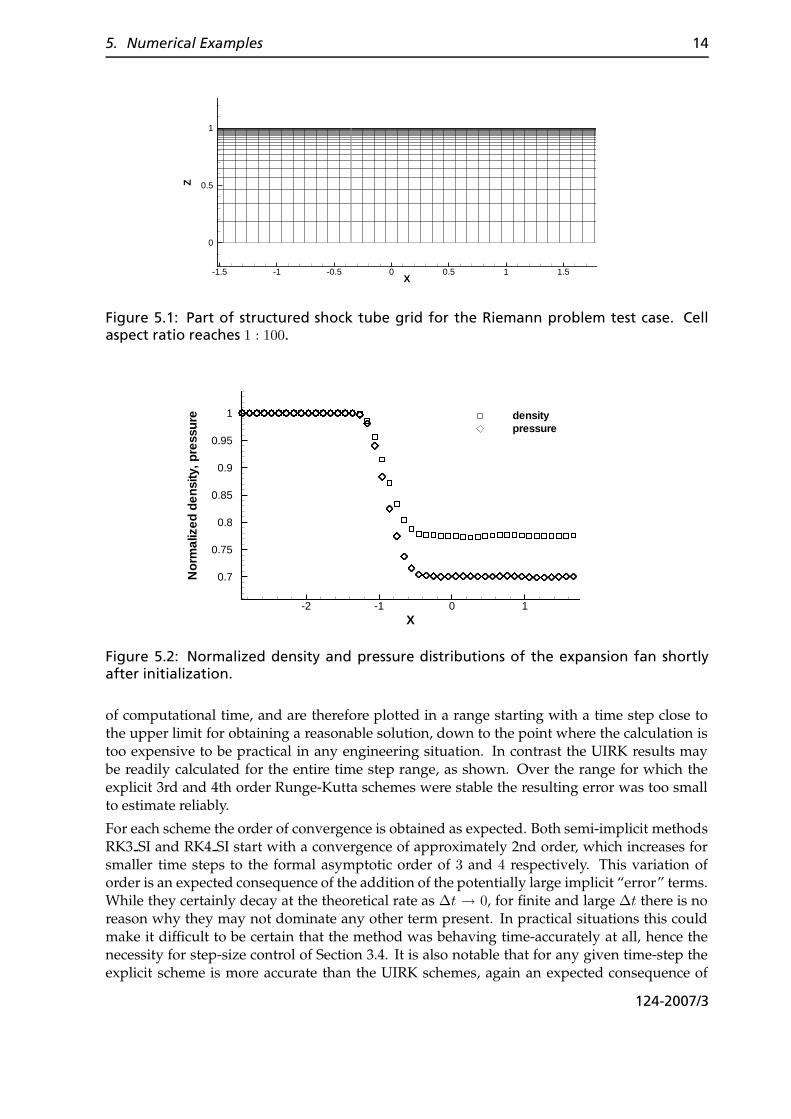
In the first test-case a Riemann problem of an expansion fan in a shock tube is simulated. Theone-dimensional solution is modelled on the two-dimensional structured grid shown in Fig-ure 5.1, which has cells varying in aspect ratio from 1 : 1 on the lower wall to 1 : 100 near theupper wall. This irregular cell distribution was chosen in an attempt to model a typical compu-tational grid, where cell sizes and aspect ratios vary significantly over the domain. Choosingan isotropic grid would favour explicit methods unrealistically, as local CFL conditions wouldlead to broadly similar time steps over the entire domain.
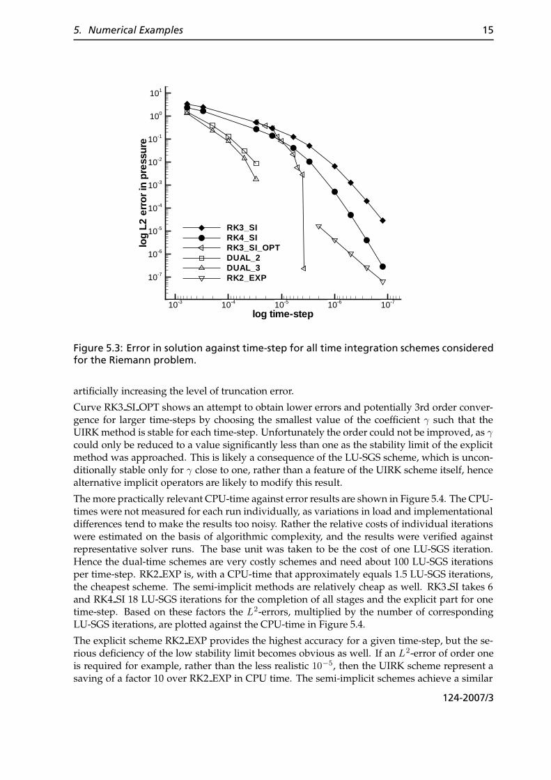
The flow is initialized as a discontinuity, and after a short time the normalized pressure anddensity are a shown in Figure 5.2. The presence of a shock in the solution was deliberatelyavoided due to spatial discretization effects such as limiter switching. The AUSM-DV schemewas used with Green-Gauss reconstruction.
A convergence study on the time step ∆t for the various schemes is depicted in Figure 5.3.The L2-error of the pressure over all points in the field is plotted logarithmically against thetime-step, so that the gradient of each curve is the achieved order of that method.
The explicit scheme RK2 EXP is plotted in the range starting with the largest stable time-stepto the point where the error can not be reliably estimated due to machine rounding errors. Bothfully implicit dual-time schemes are unconditionally stable, but require a considerable amount
13
5. Numerical Examples 14
X
Z
-1.5 -1 -0.5 0 0.5 1 1.5
0
0.5
1
Figure 5.1: Part of structured shock tube grid for the Riemann problem test case. Cellaspect ratio reaches 1 : 100.
X
Nor
mal
ized
dens
ity,p
ress
ure
-2 -1 0 1
0.7
0.75
0.8
0.85
0.9
0.95
1 densitypressure
Figure 5.2: Normalized density and pressure distributions of the expansion fan shortlyafter initialization.
of computational time, and are therefore plotted in a range starting with a time step close tothe upper limit for obtaining a reasonable solution, down to the point where the calculation istoo expensive to be practical in any engineering situation. In contrast the UIRK results maybe readily calculated for the entire time step range, as shown. Over the range for which theexplicit 3rd and 4th order Runge-Kutta schemes were stable the resulting error was too smallto estimate reliably.
For each scheme the order of convergence is obtained as expected. Both semi-implicit methodsRK3 SI and RK4 SI start with a convergence of approximately 2nd order, which increases forsmaller time steps to the formal asymptotic order of 3 and 4 respectively. This variation oforder is an expected consequence of the addition of the potentially large implicit “error” terms.While they certainly decay at the theoretical rate as ∆t → 0, for finite and large ∆t there is noreason why they may not dominate any other term present. In practical situations this couldmake it difficult to be certain that the method was behaving time-accurately at all, hence thenecessity for step-size control of Section 3.4. It is also notable that for any given time-step theexplicit scheme is more accurate than the UIRK schemes, again an expected consequence of
124-2007/3
5. Numerical Examples 15
log time-step
log
L2er
ror
inpr
essu
re
10-710-610-510-410-3
10-7
10-6
10-5
10-4
10-3
10-2
10-1
100
101
RK3_SIRK4_SIRK3_SI_OPTDUAL_2DUAL_3RK2_EXP
Figure 5.3: Error in solution against time-step for all time integration schemes consideredfor the Riemann problem.
artificially increasing the level of truncation error.
Curve RK3 SI OPT shows an attempt to obtain lower errors and potentially 3rd order conver-gence for larger time-steps by choosing the smallest value of the coefficient γ such that theUIRK method is stable for each time-step. Unfortunately the order could not be improved, as γcould only be reduced to a value significantly less than one as the stability limit of the explicitmethod was approached. This is likely a consequence of the LU-SGS scheme, which is uncon-ditionally stable only for γ close to one, rather than a feature of the UIRK scheme itself, hencealternative implicit operators are likely to modify this result.
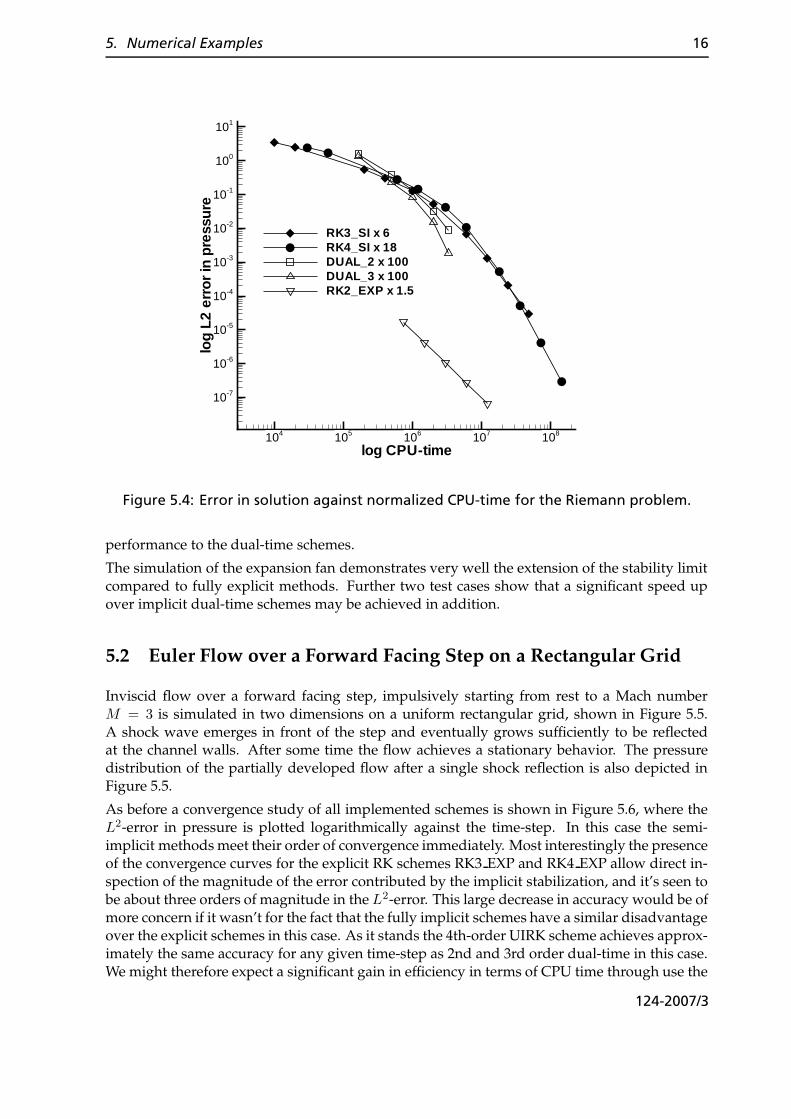
The more practically relevant CPU-time against error results are shown in Figure 5.4. The CPU-times were not measured for each run individually, as variations in load and implementationaldifferences tend to make the results too noisy. Rather the relative costs of individual iterationswere estimated on the basis of algorithmic complexity, and the results were verified againstrepresentative solver runs. The base unit was taken to be the cost of one LU-SGS iteration.Hence the dual-time schemes are very costly schemes and need about 100 LU-SGS iterationsper time-step. RK2 EXP is, with a CPU-time that approximately equals 1.5 LU-SGS iterations,the cheapest scheme. The semi-implicit methods are relatively cheap as well. RK3 SI takes 6and RK4 SI 18 LU-SGS iterations for the completion of all stages and the explicit part for onetime-step. Based on these factors the L2-errors, multiplied by the number of correspondingLU-SGS iterations, are plotted against the CPU-time in Figure 5.4.
The explicit scheme RK2 EXP provides the highest accuracy for a given time-step, but the se-rious deficiency of the low stability limit becomes obvious as well. If an L2-error of order oneis required for example, rather than the less realistic 10−5, then the UIRK scheme represent asaving of a factor 10 over RK2 EXP in CPU time. The semi-implicit schemes achieve a similar
124-2007/3
5. Numerical Examples 16
log CPU-time
log
L2er
ror
inpr
essu
re
104 105 106 107 108
10-7
10-6
10-5
10-4
10-3
10-2
10-1
100
101
RK3_SI x 6RK4_SI x 18DUAL_2 x 100DUAL_3 x 100RK2_EXP x 1.5
Figure 5.4: Error in solution against normalized CPU-time for the Riemann problem.
performance to the dual-time schemes.
The simulation of the expansion fan demonstrates very well the extension of the stability limitcompared to fully explicit methods. Further two test cases show that a significant speed upover implicit dual-time schemes may be achieved in addition.
5.2 Euler Flow over a Forward Facing Step on a Rectangular Grid
Inviscid flow over a forward facing step, impulsively starting from rest to a Mach numberM = 3 is simulated in two dimensions on a uniform rectangular grid, shown in Figure 5.5.A shock wave emerges in front of the step and eventually grows sufficiently to be reflectedat the channel walls. After some time the flow achieves a stationary behavior. The pressuredistribution of the partially developed flow after a single shock reflection is also depicted inFigure 5.5.
As before a convergence study of all implemented schemes is shown in Figure 5.6, where theL2-error in pressure is plotted logarithmically against the time-step. In this case the semi-implicit methods meet their order of convergence immediately. Most interestingly the presenceof the convergence curves for the explicit RK schemes RK3 EXP and RK4 EXP allow direct in-spection of the magnitude of the error contributed by the implicit stabilization, and it’s seen tobe about three orders of magnitude in the L2-error. This large decrease in accuracy would be ofmore concern if it wasn’t for the fact that the fully implicit schemes have a similar disadvantageover the explicit schemes in this case. As it stands the 4th-order UIRK scheme achieves approx-imately the same accuracy for any given time-step as 2nd and 3rd order dual-time in this case.We might therefore expect a significant gain in efficiency in terms of CPU time through use the
124-2007/3
5. Numerical Examples 17
Figure 5.5: Partially developed flow over a forward facing step at Mach 3, with computa-tional grid.
124-2007/3
5. Numerical Examples 18
semi-implicit scheme.
log time-step
log
L2
erro
rin
pres
sure
10-610-510-4
10-7
10-5
10-3
10-1
101
103
RK3_SIRK4_SIDUAL_2DUAL_3RK3_EXPRK4_EXP
Figure 5.6: Error in solution against time-step for all time integration schemes consideredfor the forward-facing step.
The improvement in efficiency for both semi-implicit methods is demonstrated in Figure 5.7.The accuracy of the commonly applied dual-time methods for the two largest step sizes istaken as an approximate reference point for typical engineering accuracy. In this range theUIRK schemes provide a reduction in CPU-time of a factor of 3 to 10 over the fully implicitmethods. Notable is that the 4th-order UIRK scheme looses much efficiency in comparisonto the 3rd-order scheme because of its high per-step expense, indicating that a 4th-order UIRKmethod with a significantly lower stage count would be very desirable. RK3 EXP and RK4 EXPperform also excellently here, primarily as a consequence of the uniform cell size in the mesh.
The results of the forward facing step problem demonstrate the potential of the presented meth-ods regarding stability and efficiency compared to fully implicit methods.
5.3 Euler Flow over a Ramp on a Triangular Grid
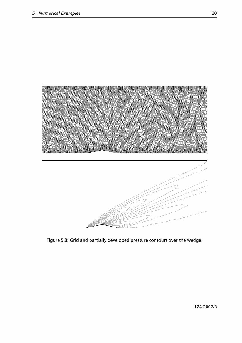
The last test case considers again impulsively started two-dimensional inviscid flow over aramp at Mach 3. In contrast to the forward facing step problem the grid consists here of tri-angles which decrease slightly in size as they approach the walls of the domain, and againwhose aspect ratios do not vary significantly. The resulting pressure distribution is plotted inFigure 5.8.
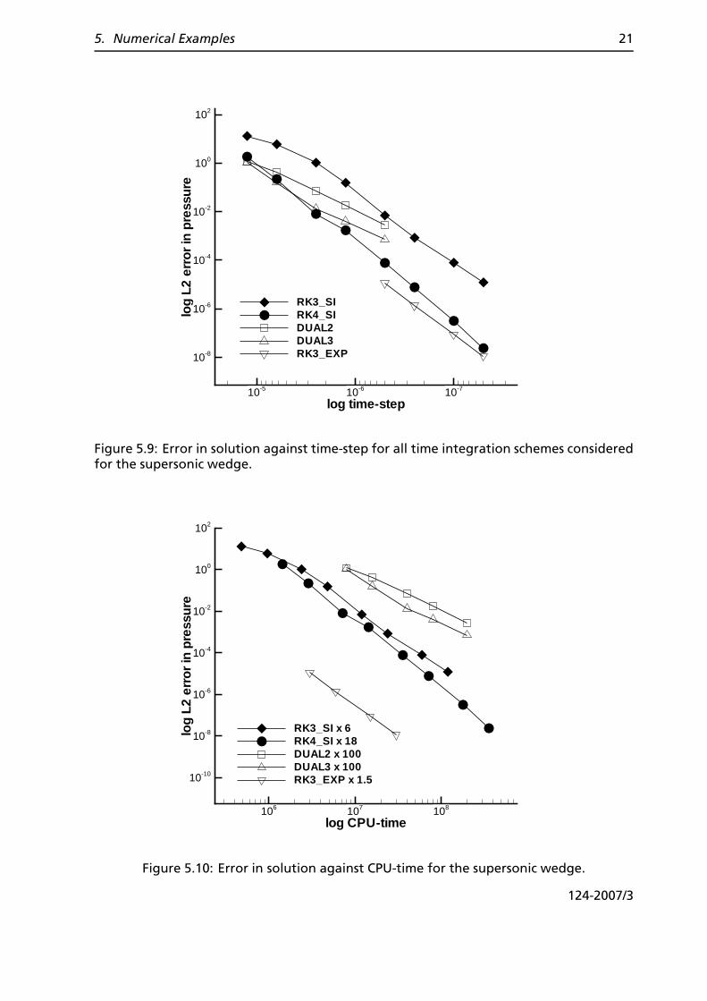
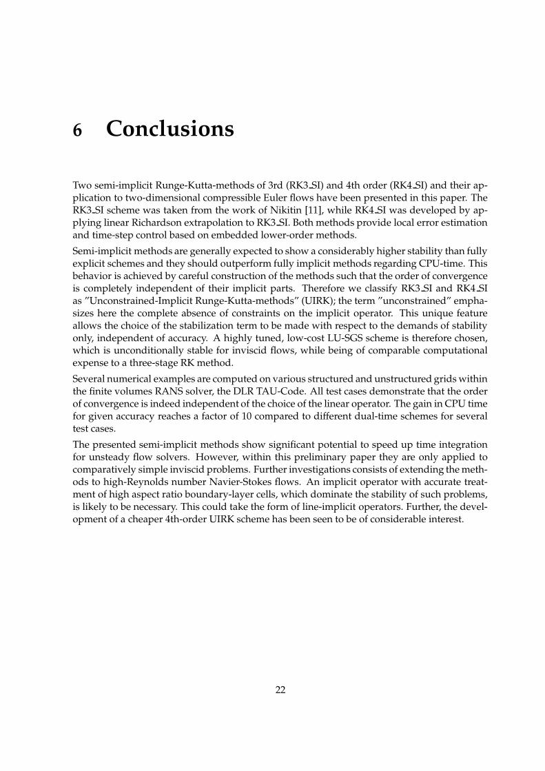
Again a convergence study was made, see Figure 5.9, where it can be seen that the 4th-ordersemi-implicit scheme perform better than both fully implicit schemes in terms of accuracy fora given time step size.
124-2007/3
5. Numerical Examples 19
log CPU-time
log
L2er
ror
inpr
essu
re
104 105 106 107
10-9
10-7
10-5
10-3
10-1
101
RK3_SI x 6RK4_SI x 18DUAL_2 x 100DUAL_3 x 100RK3_EXP x 1.5RK4_EXP x 6
Figure 5.7: Error in solution against CPU-time for the forward-facing step.
The corresponding CPU-time curves are depicted in Figure 5.10, with similar results to theprevious case. In particular the UIRK schemes still outperform dual-time by a factor of 3 to 10,and despite the variations in cell size, the explicit schemes are still significantly more efficientthan dual-time.
124-2007/3
5. Numerical Examples 20
Figure 5.8: Grid and partially developed pressure contours over the wedge.
124-2007/3
5. Numerical Examples 21
log time-step
log
L2
erro
rin
pres
sure
10-710-610-5
10-8
10-6
10-4
10-2
100
102
RK3_SIRK4_SIDUAL2DUAL3RK3_EXP
Figure 5.9: Error in solution against time-step for all time integration schemes consideredfor the supersonic wedge.
log CPU-time
log
L2
erro
rin
pres
sure
106 107 108
10-10
10-8
10-6
10-4
10-2
100
102
RK3_SI x 6RK4_SI x 18DUAL2 x 100DUAL3 x 100RK3_EXP x 1.5
Figure 5.10: Error in solution against CPU-time for the supersonic wedge.
124-2007/3
6 Conclusions
Two semi-implicit Runge-Kutta-methods of 3rd (RK3 SI) and 4th order (RK4 SI) and their ap-plication to two-dimensional compressible Euler flows have been presented in this paper. TheRK3 SI scheme was taken from the work of Nikitin [11], while RK4 SI was developed by ap-plying linear Richardson extrapolation to RK3 SI. Both methods provide local error estimationand time-step control based on embedded lower-order methods.
Semi-implicit methods are generally expected to show a considerably higher stability than fullyexplicit schemes and they should outperform fully implicit methods regarding CPU-time. Thisbehavior is achieved by careful construction of the methods such that the order of convergenceis completely independent of their implicit parts. Therefore we classify RK3 SI and RK4 SIas ”Unconstrained-Implicit Runge-Kutta-methods” (UIRK); the term ”unconstrained” empha-sizes here the complete absence of constraints on the implicit operator. This unique featureallows the choice of the stabilization term to be made with respect to the demands of stabilityonly, independent of accuracy. A highly tuned, low-cost LU-SGS scheme is therefore chosen,which is unconditionally stable for inviscid flows, while being of comparable computationalexpense to a three-stage RK method.
Several numerical examples are computed on various structured and unstructured grids withinthe finite volumes RANS solver, the DLR TAU-Code. All test cases demonstrate that the orderof convergence is indeed independent of the choice of the linear operator. The gain in CPU timefor given accuracy reaches a factor of 10 compared to different dual-time schemes for severaltest cases.
The presented semi-implicit methods show significant potential to speed up time integrationfor unsteady flow solvers. However, within this preliminary paper they are only applied tocomparatively simple inviscid problems. Further investigations consists of extending the meth-ods to high-Reynolds number Navier-Stokes flows. An implicit operator with accurate treat-ment of high aspect ratio boundary-layer cells, which dominate the stability of such problems,is likely to be necessary. This could take the form of line-implicit operators. Further, the devel-opment of a cheaper 4th-order UIRK scheme has been seen to be of considerable interest.
22
Bibliography
[1] G. Bader and P. Deuflhard. A semi-implicit mid-point rule for stiff systems of ordinarydifferential equations. Numerische Mathematik, 41:373–398, 1983.
[2] J. Blazek. Computational Fluid Dynamics: Principles and Applications. Elsevier Science, 2001.ISBN 0-08-043009-0.
[3] J. C. Butcher. The numerical analysis of ordinary differential equations: Runge-Kutta and generallinear methods. Wiley-Interscience, 1987.
[4] P. Deuflhard and F. Bornemann. Scientific Computing with Ordinary Differential Equations,volume 42 of Texts in Applied Mathematics. Springer, 2002.
[5] Richard Dwight. Efficiency Improvements of RANS-Based Analysis and Optimization usingImplicit and Adjoint Methods on Unstructured Grids. PhD thesis, School of Mathematics,University of Manchester, 2006.
[6] T. Gerhold, M. Galle, O. Friedrich, and J. Evans. Calculation of complex 3D configurationsemploying the DLR TAU-Code. In American Institute of Aeronautics and Astronautics, PaperAIAA-97-0167, 1997.
[7] E. Hairer and C. Lubich. Extrapolation of stiff differential equations. Numerische Mathe-matik, 52:377–400, 1988.
[8] A. Jameson. Time dependant calculations using multigrid with applications to unsteadyflows past airfoils and wings. AIAA Paper, AIAA-91-1596, 1991.
[9] A. Jameson, W. Schmidt, and E. Turkel. Numerical solutions of the Euler equations byfinite volume methods using Runge-Kutta time-stepping schemes. In AIAA Paper, AIAA-81-1259, 1981.
[10] P. Kaps, S.W.H. Poon, and T.D. Bui. Rosenbrock methods for stiff ODEs: A comparison ofRichardson extrapolation and embedding technique. Computing, 34:17–40, 1984.
[11] N. Nikitin. Third-order-accurate semi-implicit runge-kutta scheme for incompressibleNavier-Stokes equations. International Journal for Numerical Methods in Fluids, 51:221–233,2006.
[12] Y. Wada and M.-S. Liou. A Flux Splitting Scheme with High-Resolution and Robustnessfor Discontinuities. Collection of Papers on Aerospace Science, pages 10–13, January 1994.
[13] J.J. Yoh and X. Zhong. New hybrid Runge-Kutta methods for unsteady reactive flow sim-ulation. AIAA Journal, 42(8):1593–1600, 2004.
[14] J.J. Yoh and X. Zhong. New hybrid Runge-Kutta methods for unsteady reactive flow sim-ulation: Applications. AIAA Journal, 42(8):1593–1600, 2004.
23
BIBLIOGRAPHY 24
[15] S. Yoon and A. Jameson. An LU-SSOR scheme for the Euler and Navier-Stokes equations.AIAA Journal, 26:1025–1026, 1988.
124-2007/3
IB 124-2007/3
A Fourth Order Semi-Implicit Runge-Kutta Method for the