Mathematical Modelling and Numerical Analysis Will be set by the publisher

Modelisation Mathematique et Analyse Numerique

A MODEL OF MACROSCALE DEFORMATION AND MICROVIBRATION IN

SKELETAL MUSCLE TISSUE

Bernd Simeon1, Radu Serban2 and Linda R. Petzold3

Abstract. This paper deals with modelling the passive behavior of skeletal muscle tissue includingcertain microvibrations at the cell level. Our approach combines a continuum mechanics model withlarge deformation and incompressibility at the macroscale with chains of coupled nonlinear oscillators.The model verifies that an externally applied vibration at the appropriate frequency is able to syn-chronize microvibrations in skeletal muscle cells. From the numerical analysis point of view, one faceshere a partial differential-algebraic equation (PDAE) that after semi-discretization in space by finiteelements possesses an index up to three, depending on certain physical parameters. In this context,the consequences for the time integration as well as possible remedies are discussed.

Resume. ...

1991 Mathematics Subject Classification. 65L05, 65L80, 65M12, 65M20, 74C05.

September 27, 2008.

Introduction

Complex biological systems exhibit a great variety of phenomena that demand for appropriate mathematicalmodels and corresponding numerical simulation methods. In this contribution, we focus on the dynamics ofskeletal muscle tissue and introduce a top-down approach that combines a continuum mechanics model at themacroscopic level with clusters of oscillating cells at the microscopic level. From a mathematical viewpoint, thisapproach leads to a coupled system of transient PDEs and ODEs, which after semi-discretization in space byfinite elements turns out to be a system of index three DAEs [1].

Dating back to Hill [14] and Huxley [16], skeletal muscles have been the subject of extensive research forseveral decades. A variety of models exist [18] that can be classified in terms of biological structure, i.e., at thetissue, cell or intra-cellular scale, or in terms of mathematical properties, i.e., discrete versus continuous models.Due to limited resources and an insufficient understanding of mutual coupling mechanisms between differentlevels, however, most computational approaches have so far tended to target a relatively narrow section of thismodel hierarchy.

A new aspect comes into play when the microvibration of skeletal muscle cells is taken into account. Thisphenomenon is related to physiological tremor and features also similarities to the rhythmic excitation of cardiaccells [9]. The absence of these microvibrations in outer space missions [8] as well as in cancerous tissue indicates

Keywords and phrases: skeletal muscle tissue, microvibrations, coherence, PDAE, index, time integration

1 Zentrum Mathematik, TU Munchen, Boltzmannstr. 3, 85748 Garching, Germany2 Xulu entertainment 890 Hillview Court, Milpitas, CA 950323 Dept. of Mechanical Engineering, University of California Santa Barbara, CA 93106, USA

c© EDP Sciences, SMAI 1999

2 TITLE WILL BE SET BY THE PUBLISHER

their relevance for physiological transport processes in the extracellular matrix structure. New therapy conceptsmechanically stimulate the diseased muscle tissue and lead to a synchronization effect, also called entrainment[21]. A detailed model of the driving mechanisms based on specific parameters such as ion concentration,base-acid content or osmolarity has not been available so far.

Our goal here is to develop a simple mechanical model for the cell’s microvibrations and to demonstrate howit can be coupled with a macroscopic PDE model for the muscle tissue. The ultimate vision is to be able topredict the dynamics of vibrational therapies so that the validity of the underlying physiological assumptions canbe tested. On this road towards a realistic multi-level model, we present the first steps and also a methodologythat should be open to further extensions in the direction of systems biology. An important feature of themodel is that it can be expressed directly in the COMSOL framework [5], giving access to COMSOL’s librariesof material properties and models, and the ability to extend to complex geometries and multiphysics. Thus themodel is open towards an incorporation of greater physical or physiological details.

With respect to the underlying mathematical structures, our approach features some parallels to the Bidomainequations for the electrical activity of the heart [17]. There one has also a coupled system with a continuummodel that describes the spatial distribution of the trans-membrane potential and a set of ODEs for physiologicalparameters such as ionic fluxes and enzyme kinetics. For the computational treatment of the PDE part, theusage of the finite element method is first choice as complicated geometries need to be resolved. The systemof semi-discretized Bidomain equations forms also a DAE, but the index is one instead of three, as in ourcase where the higher index results from the equations of incompressible elasticity that are typically requiredto model muscle tissue. A closer look at the equations, however, reveals that actually the incompressibilityconstraint is weakened by a regularization term, which in turn represents a singular perturbation.

The microvibrations at the cell level are modelled in terms of a one-dimensional chain of oscillators that corre-sponds to an appropriate one-dimensional cross-section through the tissue. The oscillators possess a nonlinearityof Van der Pol type. As one of the objectives of the modeling is to determine whether an externally-drivenmicrovibration applied to the muscle tissue can cause synchronization of the cellular oscillators, we introduce ameasure of synchronization, the coherence, and record it along the simulation runs.

This paper is organized as follows: In Section 1 we introduce a constrained nonlinear PDE model of themacroscopic skeletal muscle tissue along with an ODE model of the microscale oscillating cells. We then discussthese models and their coupling. In Section 2 we examine the structure of the semi-discretized PDAE model,showing that depending on the parameters, the index can be up to three. Furthermore, we apply index reductionand explore alternative formulations to obtain a more reliable and efficient time integration. It turns out that astraightforward stabilized index-two formulation in the PDE context may lead to an incorrect implementationusing COMSOL defaults. Numerical simulations illustrating the synchronization of the oscillators and theresults of the two-dimensional PDE model are presented in Section 3. Section 4 concludes with a summary ofthe results and a discussion of future directions.

1. Skeletal Muscle Tissue Model

The behavior of skeletal muscles at the macroscale is typically described by biomechanical models that arerelated to the equations of multibody dynamics and deformable bodies. Probably the oldest approach is themodel of Hill [14], which treats the muscle as a nonlinear force law with contracting element, serial elasticelement, and parallel elastic element. It is still in wide use for biomechanical studies such as gait analysis thatare based on a multibody representation.

At the microscale, the famous model of Huxley [16] describes the activation of muscle tissue by means of thecross-bridges between actin and myosin inside each cell. During muscle contraction, a fraction of these cross-bridges is attached and subsequently released. The distribution of attached cross-bridges satisfies a transportequation that is driven by external controls and the amount of available calcium in the myofibrillar space. Sincethe solution of this first order PDE at the cell level requires a substantial computational effort, reduced ODEmodels of the actin-myosin binding have been developed [25] that can be used in combination with continuummechanics models.

TITLE WILL BE SET BY THE PUBLISHER 3

Figure 1. Skeletal muscle with detail of lateral cross section on the right

Fig. 1 shows a skeletal muscle with a detail of a lateral cross section. The muscle cells form long fibres inlongitudinal direction, and as the cross section reveals, the cells are arranged in a matrix-like structure, whichis the extracellular matrix. It consists mainly of different protein structures, in particular collagen.

In the following, we first deal with the macroscale by looking deeper into a standard continuum mechanicsapproach. Thereafter, the microscale is discussed.

1.1. A Model from Continuum Mechanics

Soft biological materials such as muscle tissue can be viewed as deformable bodies that possess a certaingeometry and specific material parameters. Several aspects deserve particular attention in the development of arealistic model. The body may undergo large deformations and rigid body motions, the constitutive law relatingstress and strain is nonlinear and often anisotropic, and the large fraction of water makes the material almostincompressible [11]. One also has to distinguish between active behavior, a contraction process controlled bythe actin-myosin binding in each cell, and passive behavior, in which the muscle tissue changes solely due toexternal forces. In this work, we restrict ourselves to passive behavior and apply next a step by step procedureto establish the model equations at the macroscale. For a general treatment of elasticity theory see [19].

Linear Elasticity, Incompressible Case

We start with the small deformation case and consider a solid that occupies the spatial reference domainΩ ⊂ R

3. A material point in cartesian coordinates is denoted by x ∈ Ω, and t ∈ [0, T ] stands for the time. Thevector field u(x, t) ∈ R

3 is the displacement of the solid body.Next, we introduce as usual the strain tensor

ε = ε(u) =1

2(∇u + ∇uT ) (1)

where ∇ = ∂/∂x, which can be viewed as a symmetric 3×3 Jacobian matrix of the displacement. Furthermore,we assume Hooke’s law

σ = σ(u) = Λ(trace ε(u))I + 2ςε(u) (2)

for the relation between strain and stress tensor σ, with 3× 3 identity matrix I and Lame constants Λ and ς asmaterial parameters. Hooke’s law will be extended below to the more general class of hyperelastic materials.

4 TITLE WILL BE SET BY THE PUBLISHER

For Hooke’s law, one may also formulate the strain energy as tensor product σ : ε = trace (σε) of stress andstrain, integrated over the whole body,

W =1

2

∫

Ω

σ : ε dx . (3)

Frequently, one makes use of an alternative notation for Hooke’s law that is based on a vector representationof the tensors σ and ε. Set

ε := (ε11, ε22, ε33, 2ε12, 2ε23, 2ε13)T , σ := (σ11, σ22, σ33, σ12, σ23, σ13)

T

and replace the Lame constants by Poisson’s number ν = Λ/(2(Λ + ς)) and modulus of elasticity E = ς(3Λ +2ς)/(Λ + ς). Hooke’s law (2) then reads σ = D ε with constant 6 × 6 matrix

D =E

(1 + ν)(1 − 2ν)

1 − ν ν νν 1 − ν νν ν 1 − ν

(1 − 2ν)/2(1 − 2ν)/2

(1 − 2ν)/2

. (4)

As inspection of matrix D shows, the case ν = 12, which in fact corresponds to incompressibility, deserves special

attention. We will come back to that point in the next paragraph. For the moment, we put everything togetherby invoking the balance of momentum and summarize the equations of motion of linear elasticity in strong formas

ρ u(x, t) = divσ(u(x, t)) + f(x, t) in Ω (5)

where σ is given by Hooke’s law (2) or (4), respectively. Furthermore, ρ is the mass density and f the vectorof internal loads.

Incompressibility

As pointed out above, for ν → 1/2 we are approaching the incompressible case where the equations (5) arenot well-defined. Biological tissue consists to 70 % or more of water, which renders such materials not fully butalmost incompressible. With respect to Poisson’s number ν, this means that ν may assume a value between0.45 up to 0.49. It is well-known that this may lead to problems such as locking and spatial oscillations withregard to the finite element approximation in space, and therefore one usually prefers a mixed formulation insuch situations.

In order to set up a mixed formulation, we introduce the scalar pressure p(x, t) as negative mean stress

p = −σ11 + σ22 + σ33

3(6)

depending on the normal stress components σ11, σ22, σ33. Thus we may rewrite Hooke’s law as

σ = σ(u, p) = Dd ε + (p, p, p, 0, 0, 0)T (7)

with deviatoric elasticity matrix Dd. Moreover, a straightforward computation shows that the definition (6) ofthe pressure can be re-expressed as the constraint equation

p

κ+ ε11 + ε22 + ε33 = 0 (8)

with bulk modulus κ = E/(3(1 − 2ν)). In the limit case ν → 12, the bulk modulus obviously tends to infinity,

which means that it may also be employed as a measure of the incompressibility as long as that limit situationis not reached.

TITLE WILL BE SET BY THE PUBLISHER 5

The definitions of the divergence and of the strain tensor immediately imply

ε11 + ε22 + ε33 = div u.

In other words, incompressibility for solids leads to the same zero divergence constraint as incompressibility forfluids. In total, we thus end up with the equations of motion in the incompressible case

ρu − divσ(u, p) = f ,pκ + div u = 0

in Ω. (9)

Finally, we apply one more transformation to obtain better insight into the structure of this PDE. Observe thataccording to (7), we can furthermore split the divergence of σ(u, p) into

divσ(u, p) = divσd(u) + ∇p,

with a deviatoric stress tensor σd. In the limit ν → 1/2, one obtains

ρu − divσd(u) −∇p = f ,div u = 0

in Ω

These equations of motion exhibit a similar structure as the Navier-Stokes equations in fluid dynamics. However,the second time derivative of the displacement is a major difference and affects the index of the DAE that resultsfrom spatial discretization, see Section 2 below.

Damping

Muscle tissue clearly features dissipative properties, and thus a reasonable model should include some kindof damping. We choose here the most widespread approach, which is Rayleigh damping. Instead of Hooke’slaw (2), one assumes in this case the stress-strain relation

σ = Λ(trace ε(u + βu))I + 2ςε(u + βu) = σ(u) + βd

dtσ(u). (10)

The parameter β ≥ 0 specifies damping depending on the body’s frequencies. With a second parameter α ≥ 0determining viscous damping, the equations of motion (5) are then rewritten as

ρ(u + αu) = divσ(u) + βdivd

dtσ(u) + f in Ω. (11)

Note that (11) refers to the standard formulation in the compressible case. For the mixed formulation with thepressure as second variable, the frequency-dependent damping term becomes

σ = σ(u, p) + βd

dtσ(u, p) = σ(u, p) + βσ(u, p).

As the stress-strain relation is linear, the differentiation with respect to time goes directly through to thedisplacement field and the pressure.

Summing up, the equations of motion including incompressibility and damping yield

ρ(u + αu) − divσ(u, p) − βdivσ(u, p) = f ,pκ + div u = 0

in Ω. (12)

Using the splitting for the stress tensor as discussed above, this is equivalent to

ρ(u + αu) − divσd(u) −∇p− β(divσd(u) −∇p) = f ,pκ + div u = 0

in Ω. (13)

6 TITLE WILL BE SET BY THE PUBLISHER

In total, we have thus a system of constrained PDEs, which can also be viewed as a PDAE (partial-differential-algebraic equation). There are several important parameters, among them in particular

• The frequency-dependent damping parameter β. If β = 0, the term with p disappears, and as we willsee below, this also affects the index of the semi-discretized system.

• The bulk modulus κ. This parameter governs the term p/κ in the incompressibility constraint. Forκ≫ 1, we obtain a singular perturbation, which in the limit leads to a change of the constraint equation,also affecting the index.

The PDAE (13) still lacks boundary and initial conditions. In practical applications, one deals with mixedDirichlet and Neumann boundary conditions for the displacement, i.e.,

u = u0 on Γ0, σ(u)n = τ on Γ1, (14)

where ∂Ω = Γ0 ∪ Γ1, u0 is a prescribed displacement, τ a prescribed surface traction, and n the outer normalvector. Similarly, initial values for the displacements and velocities can be specified. Note that the pressuretypically need not be given since it can be determined from the incompressibility constraint.

Extension to Large Deformation and Material Law of Mooney-Rivlin

Finally, we give some comments on how to include finite or large deformations in the model equations andhow to introduce appropriate hyperelastic material laws. For better readibility, we will mainly use the smalldisplacement case (13) as basic model in the following, but the 2D simulations we will present in the last sectionare actually based on the hyperelastic material law of Mooney-Rivlin and include large deformations.

For the purpose of modelling large deformation and hyperelastic material laws, it is convenient to use theright Cauchy-Green tensor

C = C(u) = (I + ∇u)T (I + ∇u) (15)

instead of the linear strain tensor ε from (1). The first two invariants of this symmetric 3 × 3 matrix are

I1 = trace C = C11 + C22 + C33, I2 =1

2(I2

1 − trace C2).

With these quantities, the strain energy function of a material of a Mooney-Rivlin type, which includes rubber-like soft materials, reads [5]

WMR = c10(I1 − 3) + c01(I2 − 3) +1

2κ(J − 1)2 (16)

where J = det (I + ∇u), I1 = I1J2/3, I2 = I2J

−4/3, and c10, c01 are material constants. Notice the bulkmodulus κ in the last term of (16), which stands for the volume change of the material.

Defining the first Piola-Kirchhoff stress tensor by

P (u) :=∂WMR

∂∇u, (17)

the equations of motion in the large-deformation case can be expressed by

ρ u(x, t) = divP (u(x, t)) + f(x, t) in Ω. (18)

In comparison to the equations of small deformation (5), the only difference is in the stress tensor P and itsnonlinearity. In a finite element code, the derivatives in (17) are typically computed by symbolic differentiation.

To account additionally for incompressibility, the pressure is related to the volume change through theequation

p = −κ(J(u) − 1). (19)

TITLE WILL BE SET BY THE PUBLISHER 7

Recall that J(u) = det (I +∇u), which means that for J = 1 we obtain the incompressible case. For a materiallaw of Mooney-Rivlin type, the strain energy function is then replaced by

WMR = c10(I1 − 3) + c01(I2 − 3) − p(J − 1) −p2

2κ. (20)

Upon insertion of the pressure from (19), the definition (20) becomes the original strain energy function (16).The first Piola-Kirchhoff stress tensor (17) is now a function P = P (u, p) of both displacement and pressure,and overall we get the equations of motion

ρu − divP (u, p) = f ,pκ + J(u) − 1 = 0

in Ω. (21)

Since the determinant J is a nonlinear function of ∇u, the incompressibility constraint in (21) is nonlinear ingeneral.

Finally, frequency-dependent damping can be included in the large deformation model by using

P = P (u, p) + βd

dtP (u, p)

instead of P . Viscous damping, on the other hand, is introduced in the same way as in the small deformationcase. We skip the display of the corresponding PDE system as this provides no further insight.

1.2. Modelling of Microvibrations

Microvibration of skeletal muscle cells is a phenomenon which is related to physiological tremor and whichfeatures also similarities to the rhythmic excitation of cardiac cells. The absence of these microvibrations inouter space missions as well as in cancerous tissue indicates their relevance for physiological transport processesin the extracellular matrix structure. Citing from [8,9], we summarize the experimental findings in the followingstatements:

• From these results it would appear that a low damped 7-13 Hz resonance process exists in relaxed muscle

tissue, which physiologically becomes stimulated by cardiac and muscle forces.

• Microvibrations and postural tremor were demonstrated to be strongly influenced by the presence or

absence of the earths gravitational field.

The hypothesis for the vibrational therapy of [21] is that these microvibrations are a pumping mechanismfor nutrients. On the other hand, the absence of vibrations leads to malfunctioning and disease. Mechanicalstimulation of the diseased muscle tissue in turn leads to a synchronization effect, also called entrainment, thatnormalizes the cellular rhythmicity and the nutrient flow in the extracellular matrix. This hypothesis suggeststhat there is a direct link to the mathematical theory of nonlinear oscillators and their synchronous coupling.

A detailed model of the microvibration should be based on specific parameters of the extracellular matrixwhich interconnects the cells and serves as transport medium for nutrients and by-products. Among theseparameters are the temperature, ion concentration, osmolarity, base-acid content, susceptibility, and the di-electricity. However, though nonlinear oscillators are a common phenomenon in biological systems and havebeen studied at different levels, a physiologically motivated bio-chemical model of this particular process is notknown so far. An overview of existing models for cellular rhythms is found in Goldbeter [13].

Instead of tackling the complex bio-chemistry of the extracellular matrix, we concentrate here on the ob-servation that the microvibration leads to a small oscillating displacement of each cell. This displacement canbe modelled in a descriptive approach, which results in a simple mechanical model that in future work shouldbe extended to include physiological parameters and reactions. The ultimate goal is to be able to predict thedynamics of vibrational therapies so that the validity of the underlying physiological assumptions can be tested.

8 TITLE WILL BE SET BY THE PUBLISHER

Oscillator Model

We consider a one-dimensional chain of N interacting cells. The basic model for the oscillatory motion ofeach cell is inspired by a mechanical viewpoint and has been studied, among others, by Matthews et al. [20]and Cross et al. [6]. Our oscillator model is given by

yn + ω2nyn − µ(1 − y2

n)yn + ay3n −Dn

(

1

2(yn+1 + yn−1)

)

= 0, (22)

where yn(t) is the displacement of cell n with respect to a reference position. The first three terms of the modelform a Van der Pol oscillator with parameter µ while the next term ay3

n describes a stiffening of the associatedspring, related to a Duffing oscillator. In our computations, we have taken a = 0. The last term represents anearest neighbour coupling between the oscillators, which depends directly on the positions of the neighbours.We set Dn = Dωn for the coupling strength, where ωn is the natural frequency of the n-th oscillator and D aglobal parameter.

The one-dimensional chain corresponds to an appropriate one-dimensional cross-section through the tissue.A straightforward extension would be to study a two-dimensional array of oscillators, which would lead to asimilar set of equations for each oscillator and each coordinate direction [7].

One of the objectives of the modeling is to determine whether an externally-driven microvibration applied tothe extracellular matrix can cause synchronization of the cellular oscillators. Thus, a measure of synchronization,or coherence, is needed. A commonly used measure of coherence for both mechanical and cellular oscillators isthe complex order parameter Ψ

Ψ = R expiΘ =1

N

N∑

n=1

rn expiθn . (23)

In this paper, rn and θn are obtained by local transformation of the position yn and scaled velocity yn/ωn ofeach cell into polar coordinates. We expect that R, which measures in a sense the net strength of the chainof oscillators, may be useful in feedback to the model of the extracellular matrix. However, we are not in aposition at the present time to model that feedback, due to a lack of physiological data.

To measure only the phase coherence, we form χ := 1N

∑Nn=1 expiθn by setting rn = 1 in (23), in which case

R = 1 represents perfect coherence and R = 0 indicates a complete lack of coherence.

1.3. Coupling Macro- and Microscale

We next discuss the coupling of both the PDE model for the muscle tissue and the oscillator chain formicrovibrations.

One-way Coupling

In one-way coupling, the motion at the macro-scale is not affected by the microvibrations, which means thatthe PDE (13) is solved separately and its solution used as input to the oscillator chain. This leads to thequestion of how to model the coupling via some kind of forcing function.

In our studies, we chose

yn + ω2nyn − µ(1 − y2

n)yn + ay3n −Dn

(

1

2(yn+1 + yn−1)

)

+ c(u) = 0, (24)

with an additional periodic internal coupling by taking D1(y2 + yN )/2 as coupling term for y1 and DN (y1 +yN−1)/2 as coupling term for yN . The forcing function c(u) evaluates the displacement at some point ξ (e.g.,a quadrature node) and time t. E.g., a straightforward proportional forcing in the vertical direction reads

c(u) = γ · uy(ξ, t)

TITLE WILL BE SET BY THE PUBLISHER 9

where uy is the y-component of the displacement and γ a parameter.This approach is inspired by the structure of the muscle tissue, which consists of the extracellular matrix

and the cells in between. The matrix, a truss-like structure, is mainly composed of collagen and determines thematerial properties, compare Fig.1. External vibrations will travel through the matrix and reach the cells viathe matrix. Due to the tiny length scale at the cell level, the assumption of a simultaneous forcing of a clusterof cells is justified.

Other possible choices are a forcing of the boundary oscillators y1 and yN only.

Two-way Coupling

Since we lack a detailed model at the cell level, we only discuss here possible approaches for a two-waycoupling. The hypothesis in the vibrational therapy is that the muscle tissue starts to relax when the cellsoscillate in a coherent way, which coressponds to a healthy state. In case of no or unsynchronized oscillations,one suspects a hardening effect which makes the tissue stiffer. In our model, this would mean a dependence ofmaterial parameters such as the elasticity modulus on the coherence of the microvibrations, i.e.

E(x, t) = c(y, t;x)

where y = (y1, . . . , yN ) are the oscillators on the microscale around point x.If one applies the finite element method to discretize the model with such functions for material parameters

the integrals in the weak form need to be approximated by appropriate quadrature rules, which means that werequire the evaluation of E(ξj , t) = c(y, t; ξj) at each quadrature point ξj . This coupling mechanism resemblesapproaches for simulating muscle contraction [11] and is also related to multiscale modelling in the materialssciences.

2. Structure of the Semidiscretized Equations

The PDAE (13) is now discretized in space by applying the finite element method. Due to the mixedformulation, we approximate both the displacement field and the pressure by apppropriate basis functions,

u(x, t).=

nq∑

i=1

φi(x)qi(t), p(x, t).=

nλ∑

j=1

ψj(x)λj(t), (25)

with unknown nodal coefficient vectors q(t) ∈ Rnq and λ(t) ∈ R

nλ . The structure and the index of the resultingDAE depend on the choice of the basis functions φi and ψj and on the material parameters, in particular thebulk modulus κ and the damping coefficient β.

2.1. Structure of Matrices and Full Rank Criterion

We skip the display of the weak form of (13) and proceed directly with the DAE that results from the finiteelement approximation (25). This DAE can be written as

Mq + Aq + BT λ + Dq + βBT λ = f(t),− 1

κMpλ + Bq = 0.(26)

Here,

M :=

(∫

Ω

ρφi(x)T φj(x) dx

)

i,j=1:nq

and Mp :=

(∫

Ω

ψi(x)ψj(x) dx

)

i,j=1:nλ

are the mass matrices for displacement and pressure, respectively. The stiffness matrix is given by

A :=

(∫

Ω

σd(φi(x)) : ε(φj(x)) dx,

)

i,j=1:nq

,

10 TITLE WILL BE SET BY THE PUBLISHER

while the constraint matrix is obtained from

BT :=

(∫

Ω

div ϕi(x) · ψj(x) dx

)

i=1:nq,j=1:nλ

.

Finally, the damping matrix is a simple linear combination D = αM + βA.For standard finite elements, the mass matrices for displacement and pressure are symmetric positive definite

while the stiffness matrix is positive semi-definite. Of particular interest is the nλ × nq constraint matrix B,as we require it below to be of full rank. Clearly, the dimension nλ of the constraints must be less than thedimension of the displacement variables nq.

We can express the full rank requirement in terms of the singular values of B, which are given by the singularvalue decomposition [12, §2.5]

UT BV = diag (σ1, . . . , σnλ) ∈ R

nλ×nq

with orthogonal matrices U ∈ Rnλ×nλ and V ∈ R

nq×nq . The singular values are ordered as

σ1 ≥ σ2 ≥ . . . ≥ σnλ≥ 0 ,

and for the full rank of B we require σmin := σnλ> 0. Observe that

λT BBT λ

λT λ=

τT diag (σ21 , . . . , σ

2min

)τ

τT τ≥ σ2

min

for λ 6= 0 and τ := UT λ. In case of τ = (0, . . . , 0, 1)T ∈ Rnλ , this inequality is sharp and we conclude

σ2min

= minλ

λT BBT λ

λT λ⇐⇒ σmin = min

λ

‖BT λ‖2

‖λ‖2

.

Moreover, using the definition of the operator norm we get the identity

‖BT λ‖2 = maxv

‖vT BT λ‖2

‖v‖2

= maxv

λT Bv

‖v‖2

since ‖vT BT λ‖2 = |λT Bv|. Overall, we have thus derived the minimax characterization [22]

minλ

maxv

λT Bv

‖λ‖2‖v‖2

= σmin(B) > 0 (27)

as equivalent to the full rank criterion. It is important to realize that (27) is nothing else than the discrete inf-sup condition of mixed and hybrid finite element analysis [4]. If the basis functions φi and ψj in (25) satisfy theinf-sup condition, i.e., they are ”well-balanced” in the finite element sense, then the full rank of the constraintmatrix B is guaranteed. In our specific application, the Taylor-Hood ”P2-P1” combination with quadraticsfor the displacements and linears for the pressure is well-known to be a stable pairing for which the inf-supcondition holds.

2.2. Index of Semi-discretized Equations

We begin with the small-deformation case, which after semi-discretization yields the DAE (26), assumingthe full rank condition (27) for the constraint matrix B to hold. The semi-explicit structure of the equationssimplifies the analysis greatly, and we can draw on well-known results from the field of mechanical multibodysystems, which basically lead to the same structure [22].

TITLE WILL BE SET BY THE PUBLISHER 11

Case κ = ∞: In the purely incompressible case, the term κ−1Mpλ in the constraint equation disappears.If additionally β = 0, the equations (26) have exactly the same structure as in multibody dynamics, andaccordingly the index is three. However, for frequency-dependent damping with β > 0, the index drops to twosince the term βBT λ in the dynamic equations reduces the number of differentiation steps that are necessaryto generate an ODE for λ by one.

Case κ <∞: For finite bulk modulus, the constraint equation can be rewritten as

Mpλ = κBq.

As the mass matrix for the pressure is invertible, we can thus directly solve for λ = λ(q), which means thatthe index amounts to one in this case, regardless of the damping parameter β. Though this seems a favorablesituation, one should be careful here as a large value of κ leads to a singularly perturbed system that is closeto a higher index system. Depending on the tolerances and norms used, the time integration will reflect thatcloseness or not.

From a physical point of view, we note that deformable solids always exhibit some frequency-dependentdamping. Moreover, muscle tissue is not fully incompressible, and accordingly, in practical simulations one willtypically use a finite bulk modulus κ and a damping parameter β > 0. Thus the regularization has a solidphysical basis.

Next, we turn to the large deformation case (21), where the semi-discretization by finite elements introducesadditional nonlinearities. We summarize here the structure of the resulting equations as they are generated inthe COMSOL package [5]. COMSOL utilizes velocity variables v = q to obtain a first order system, which inthe case β = 0 reads

q = v,Mv = fa(q,λ) − αMv + f c(t),

0 = − 1κMpλ + j(q).

(28)

Here, the force term fa is the discretized analogue of the Piola-Kirchhoff stress tensor P (u, p), the functionj(q) corresponds to the determinant J(u) − 1 in (21), and f c is the load vector.

If frequency-dependent damping is included, i.e., β > 0, COMSOL treats the derivative λ as an additionalunknown µ, which results in an extended system

q = v,

λ = µ,Mv = fa(q,λ) − αMv + βf b(q,v,µ) + f c(t),

0 = − 1κMpλ + j(q),

(29)

where f b corresponds to the evaluation of ddtP (u, p).

With respect to the index, the two DAEs (28) and (29) require a separate discussion.Case β = 0 and formulation (28): An appropriate linearization reduces (28) to the linear DAE (26) with

β = 0, which means that the index analysis from above remains valid. For bulk modulus κ = ∞, the index isthree, otherwise one.

Case β > 0 and formulation (29): Upon linearization of (29) we obtain

q = v,

λ = µ,

Mv = −Aq − BT λ − Dv − βBT µ + f(t),0 = − 1

κMpλ + Bq.

(30)

For finite bulk modulus κ <∞, we perform one differentiation step for the constraint and get

Mpλ = Mpµ = κBv.

12 TITLE WILL BE SET BY THE PUBLISHER

DAE κ β Index(26) ∞ 0 3(26) <∞ 0 1(26) ∞ > 0 2(26) <∞ > 0 1(28) ∞ 0 3(28) <∞ 0 1(29) ∞ > 0 3(29) <∞ > 0 2

Table 1. Dependence of the index on the formulation and the parameters. We note that(26) corresponds to the small-deformation model, whereas (28) and (29) correspond to thelarge-deformation model.

The extra multiplier µ requires now a second differentiation to generate an ODE, and the index of the systemis two. However, note that the original multiplier λ is still an index-one variable. A similar argumentation forκ = ∞ shows that the index is three in that case, with µ as index-three variable and λ as index-two variable.To summarize, the introduction of the additional multiplier µ and the corresponding differentiation in (29) raisethe index by one. Table 1 gives a compilation of these findings. It is interesting to note that in the limit asκ → ∞ and β → 0, the index of (29) is four. In the next section, we will present statistics of simulation runsby DASPK [3] for the different cases and discuss how the time integration is actually affected.

The practical question is: how should we formulate the DAE for efficient and reliable numerical solution?It is common knowledge in DAEs that there are some formidable difficulties in treating higher-index systemsdirectly. Systems of index one, and to some extent also semi-explicit systems of index two, however, can besolved by methods such as the BDF [2].

As seen above, regularization with physically meaningful values of κ and β lowers the index. There is somecause for concern about relying on the regularization to reduce the index, however, because it is possible thatthe DAE solver will struggle with the regularized system for basically the same reasons that it fails for thelimiting higher-index system.

Another possibility is to reduce the index by differentiating the constraints. Omitting the damping terms inthe linearized equations (26), this results in

Mq + Aq + BT λ = f ,Bq = 0,

(31)

which is of index two. Due to the differentiation, we lose the information of the original constraint, which isnegligible as long as the constraints are linear, but will lead to some drift away from the constraints in thelarge-deformation case.

When using a sophisticated finite element package such as COMSOL for the generation of the matrices andthe evaluation of the semidiscretized equations, it is usually very difficult or even impossible to intervene inorder to set up an index-reduced formulation such as (31) and pass it to the time integrator. It thus seems anatural idea to introduce the new formulation already at the PDE level and to let the finite element solver takecare of the remaining steps. A PDE model that corresponds to the index-two system (31) reads

ρu − divσd(u) −∇p = f ,div u = 0

in Ω. (32)

In the next section, we will compare the nonlinear analogue of (32) with the results obtained by the regularizedformulations.

TITLE WILL BE SET BY THE PUBLISHER 13

Finally, one might reasonably wonder, why not consider a stabilized index-reduction such as that describedin [10], which eliminates the possibility of drift away from the original constraint. For (31), this leads to

Mq = Mq − BT µ,

Mv = f − Aq − BT λ,0 = Bq,0 = Bv.

(33)

This formulation is based on a transformation to first order with velocity variables v, in combination withadditional constraints on the velocity level and corresponding multipliers µ. It is easy to show that µ = 0 forthe exact solution and that the index of (33) is two. The stabilized formulation (33) corresponds to the PDE

ρu = ρw + ∇r,ρw − divσd(u) −∇p = f ,

div w = 0,div u = 0,

in Ω (34)

with extra pressure variable r. Assuming sufficient smoothness, we then have

0 = div w = div u −1

ρdiv ∇r =

1

ρ∆r.

The desired conclusion r = 0 is obviously not straightforward and requires additional information such asboundary conditions, which gives a hint that the stabilization at the PDE level is not as easy as it seems.

The stabilized PDAE (34) can be directly specified in COMSOL using the multiphysics mode to define theextra variables and the ”Weak Form” option to define the equations. However, in our tests the discretizationdid not yield a system of exactly the form (33) but with a different constraint matrix B 6= B for the extramultiplier µ. This was due to the fact that COMSOL discretizes the extra multiplier using quadratic finiteelements, while the original multiplier is treated by linear finite elements. Thus the additional multplier µ isnot uniquely zero, and in fact this approach yields an incorrect solution. We were not able, using COMSOLdefaults, to change the discretization of r to a linear ansatz.

3. Computational Results

In this section, we report on the simulations that were performed. We start with a study of the oscillatorchain in a simplified setting and then continue with a 2D model for the muscle tissue that was solved by meansof COMSOL and DASPK [3].

3.1. Oscillator Chain

In order to observe a synchronization process, it is usually necessary to perform long-time simulations overmany periods of oscillation. Since this is rather costly in combination with a two-dimensional finite elementmodel, we first developed a simplified one-dimensional model for the macroscale that is based on the lineardamped wave equation

ρ(u(x, t) + αu(x, t)) = EAuxx(x, t) + βEAuxx(x, t). (35)

Here, u(x, t) is the longitudinal displacement of a thin rod of length L, E the elasticity modulus, A the crosssection area, and ρ the mass density. As boundary conditions, we consider a fixed left end where u(0, t) = 0and a right end subject to an external load, ux(L, t) = τ(t) with τ(t) being a sinusoidal signal oscillating at8 Hz. This signal travels through the rod and thus reaches all material points. The displacement u(L/2)of the midpoint serves as input to the term c(u) in the one-way coupling (24). Thus we investigate a singlerepresentative area of the tissue around the midpoint and use there the oscillator chain as a refined model.

14 TITLE WILL BE SET BY THE PUBLISHER

−3 −2 −1 0 1 2 3−3

−2

−1

0

1

2

3t = 199.4

−3 −2 −1 0 1 2 3−3

−2

−1

0

1

2

3t = 199.44

−3 −2 −1 0 1 2 3−3

−2

−1

0

1

2

3t = 199.48

−3 −2 −1 0 1 2 3−3

−2

−1

0

1

2

3t = 199.52

Figure 2. Snapshots of the positions of 20 oscillators in the complex plane. Each circle denotesone oscillator. The big dot is the common centroid.

The discretization of (35) by linear finite elements results in a system of second order ODEs

Mq + Aq + Dq = f(t) (36)

that can be integrated by standard MATLAB solvers such as ode15s. Simultaneously, the oscillator equations(24) are integrated and the coherence measure (23) is computed at each timestep. In the beginning, the systemis assumed to be at rest, which means that zero initial values for the displacements and for the oscillators arechosen. The sinusoidal input signal τ(t) is then slowly increased by means of a shifted sigmoid function.

The following data (in dimensionless form) were used to generate the solutions displayed in Figs. 2 and 3.The material parameters are EA = 1.E6, ρ = 1.E3, L = 0.1, α = 0.25, β = 0.001, and 10 finite elements wereapplied. For the oscillator model, the basic frequency was set to ωn = 16π+ ξn with ξn being a random numberin the interval [−0.05, 0.05], generated by MATLAB’s rand command. The Van der Pol parameter was set toµ = 2 for all oscillators, the cubic Duffing term disabled, and the coupling to the nearest neighbours enforcedby Dn = D · ωn with D = 3. The simulation interval was [0, 200].

For N = 20 coupled oscillators, Fig. 2 shows the synchronization that can be observed. By transformationof the position yn and the scaled velocity yn/ωn of each oscillator into polar coordinates and marking theirposition in the complex plane, one gets an impression how the oscillators travel in a group clockwise around theorigin. The extra marker stands for the position of the coherence parameter Ψ from (23), which is the commoncentroid of the oscillators. The synchronization is strong, but not optimal, which can be seen in Fig. 3. Afterthe initial acceleration phase due to the sigmoid function, the absolute value |Ψ| decreases according to thedifferent natural frequencies, and later the nonlinear synchronization comes into play and reaches a constantlevel. In the complex plane, the values of Ψ first spiral outwards from the origin and later on travel around it.

We remark that the degree of synchronization depends strongly on the chosen data. E.g., selecting a widerrange of natural frequencies or a smaller coupling parameter D will lead to a smaller coherence.

TITLE WILL BE SET BY THE PUBLISHER 15

0 50 100 150 2000

0.5

1

1.5

2

2.5

time t

radii rn

0 50 100 150 2000

0.2

0.4

0.6

0.8

1

1.2

time t

phase coherence χ

0 50 100 150 2000

0.5

1

1.5

2

time t

coherence abs(ψ)

−2 −1 0 1 2−2

−1

0

1

2ψ in complex plane

Figure 3. Radii rn and evolving coherence Ψ of the oscillators

Figure 4. Finite element mesh and boundary conditions.

3.2. Two-dimensional Model

The geometry of the two-dimensional model is displayed in Fig. 4, along with the finite element meshgenerated by COMSOL. As boundary conditions (14), two segments at both ends are kept fixed with zerodisplacement, and in the middle a surface load τ (t) = (0, τy(t)) is applied in the vertical direction, with τy(t)being again a sinusoidal signal oscillating at 8 Hz. For a refined model including a surface load that mimicksthe vibrational therapy of [21] and modified boundary conditions for the tendons see [24].

16 TITLE WILL BE SET BY THE PUBLISHER

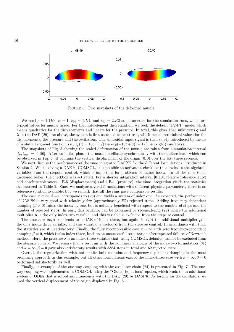
Figure 5. Two snapshots of the deformed muscle.

We used ρ = 1.1E3, α = 1, c10 = 1.E4, and c01 = 2.E2 as parameters for the simulation runs, which aretypical values for muscle tissue. For the finite element discretization, we took the default ”P2-P1” mode, whichmeans quadratics for the displacements and linears for the pressure. In total, this gives 1545 unknowns q andλ in the DAE (29). As above, the system is first assumed to be at rest, which means zero initial values for thedisplacements, the pressure and the oscillators. The sinusoidal input signal is then slowly introduced by meansof a shifted sigmoid function, i.e., τy(t) = 100 · (1/(1 + exp(−10t+ 8)) − 1/(1 + exp(8))) sin(16πt).

The snapshots of Fig. 5 showing the scaled deformation of the muscle are taken from a simulation interval[t0, tend] = [0, 50]. After an initial phase, the muscle oscillates synchronously with the surface load, which canbe observed in Fig. 6. It contains the vertical displacement of the origin (0, 0) over the last three seconds.

We next discuss the performance of the time integrator DASPK for the different formulations introduced inSection 2. When solving a DAE in COMSOL, it is possible to activate a checkbox that excludes the algebraicvariables from the stepsize control, which is important for problems of higher index. In all the runs to bediscussed below, the checkbox was activated. For a shorter integration interval [0, 10], relative tolerance 1.E-3and absolute tolerances 1.E-5 (displacements) and 1.E-1 (pressure), the time integration yields the statisticssummarized in Table 2. Since we analyze several formulations with different physical parameters, there is noreference solution available, but we remark that all the runs gave comparable results.

The case κ <∞, β = 0 corresponds to (28) and yields a system of index one. As expected, the performanceof DASPK is very good with relatively few (approximately 2%) rejected steps. Adding frequency-dependentdamping (β > 0) raises the index by one, but is actually beneficial with respect to the number of steps and thenumber of rejected steps. In part, this behavior can be explained by reconsidering (29) where the additionalmultiplier µ is the only index-two variable, and this variable is excluded from the stepsize control.

The case κ = ∞, β > 0 leads to a DAE of index three, but again, in (29) the additional multiplier µ isthe only index-three variable, and this variable is excluded from the stepsize control. In accordance with that,the statistics are still satisfactory. Finally, the fully incompressible case κ = ∞ with zero frequency-dependentdamping β = 0, which is also index three, leads to an unsuccessful termination after repeated failures of Newton’smethod. Here, the pressure λ is an index-three variable that, using COMSOL defaults, cannot be excluded fromthe stepsize control. We remark that a test run with the nonlinear analogue of the index-two formulation (31)and κ = ∞, β = 0 gave also satisfactory results with 3384 steps in total and 62 rejected steps.

Overall, the regularization with both finite bulk modulus and frequency-dependent damping is the mostpromising approach in this example, but all other formulations except the index-three case with κ = ∞, β = 0performed satisfactorily as well.

Finally, an example of the one-way coupling with the oscillator chain (24) is presented in Fig. 7. The one-way coupling was implemented in COMSOL using the ”Global Equations” option, which leads to an additionalsystem of ODEs that is solved simultaneously with the DAE (29) by DASPK. As forcing for the oscillators, weused the vertical displacement of the origin displayed in Fig. 6.

TITLE WILL BE SET BY THE PUBLISHER 17

Figure 6. Vertical displacement and pressure in the origin (0, 0).

DAE κ β Index # steps # NRJ # NCF(28) 1.E5 0 1 3275 76 0(29) 1.E5 0.0001 2 2765 64 0(29) ∞ 0.0001 3 3374 69 0(28) ∞ 0 3 362–terminated 26 10

Table 2. Statistics data from COMSOL runs. NRJ = Number of rejected steps, NCF =Number of convergence failures

In this example, we set N = 5 for the oscillators and again varied the basic frequency via ωn = 16π + ξnwith ξn being a random number in the intervall [−0.5, 0.5]. The Van der Pol parameter was set to µ = 2 for alloscillators, the cubic Duffing term disabled, and the coupling to the nearest neighbours enforced by Dn = D ·ωn

with D = 3. The simulation intervall was [0, 50]. As can be observed in Fig. 7, the synchronization shows abehavior similar to that of the one-dimensional case.

Since the plots in this section contain mainly static information and only partially reflect the dynamics of thesystem, we also generated several animations that illustrate the model and that are available for download at thewebsite [23]. The movie named musclemovie is an animation of the two-dimensional muscle model, showing thetotal deformation and how the external excitation acts on the structure, cf. Fig. 5. The movie musclehardeningcontains a refined simulation of [24] where the material parameters of the muscle were changed in a region inthe interior. In this way, hardening of muscle tissue and the effect of incoming waves from the excitation canbe analysed. The last movie chainmovie is an animation of the snapshots presented in Fig. 2 and shows howthe oscillators travel in a group in the complex plane.

4. Conclusions and Outlook

In this work, we have developed a model for the passive behavior of skeletal muscle tissue including mechanicalmicrovibrations at the cell level. With respect to the model, we were able to verify the synchronization at themicro-scale based on one-way coupling with a finite element simulation at the macro-scale. This supportsthe underlying hypothesis of vibrational therapies that cellular rhythmicithy can be stimulated by externalexcitation. What still needs to be developed is a more detailed model of the extracellular matrix, whichinterconnects the cells and serves as transport medium for nutrients and waste products.

With respect to numerical analysis, we have seen that incompressible or nearly incompressible solids leadto an intricate PDAE, whose index, after semi-discretization in space by mixed finite elements, depends ontwo specific parameters, the bulk modulus and the amount of frequency-dependent damping. For physicallymeaningful values of the parameters, which correspond to a system of index one, the time integration by DASPKperformed best, but even for the limit cases that correspond to higher index formulations, the peformance was

18 TITLE WILL BE SET BY THE PUBLISHER

0 10 20 30 40 500

0.5

1

1.5

2

2.5

3

time t

radii rn

0 10 20 30 40 500

0.2

0.4

0.6

0.8

1

1.2

time t

phase coherence χ

0 10 20 30 40 500

0.5

1

1.5

2

2.5

time t

coherence abs(ψ)

−2 −1 0 1 2−2

−1

0

1

2ψ in complex plane

Figure 7. One-way coupling with phase coherence χ and coherence Ψ.

satisfactory. The only exception is the pure index-three case with infinite bulk modulus and vanishing dampingparameter. In this context, the stabilization (34) should be further investigated, as well as the apparentlystabilizing role of the damping parameter.

Finally, using COMSOL as computational platform gives us the ability to extend the model towards anincorporation of greater physical or physiological details.

Acknowledgements

We gratefully acknowledge the work of S. Thiemann and F. Dietrich on earlier versions of the tissue and theoscillator model. Furthermore, we thank U. Randoll for initiating this investigation at the interface betweenmathematics, computer science and medical research. J. Ystrom of COMSOL AB gave us also valuable hintson specific implementation details.

References

[1] Ascher, U., Petzold, L.: Computer Methods for Ordinary Differential Equations and Differential-Algebraic Equations. SIAM

1998

[2] Brenan, K.E., Campbell, S.L., Petzold, L.R.: The Numerical Solution of Initial Value Problems in Ordinary Differential-

Algebraic Equations. SIAM 1996

[3] Brown, P., Hindmarsh, A., Petzold, L.R.: Using Krylow methods in the solution of large-scale differential-algebraic systems.

SIAM J. Sci. Comp. 15(6), 1467-1488 (1994)

[4] Brezzi, F., Fortin, M.: Mixed and Hybrid Finite Element Methods. Springer 1991

[5] COMSOL Multiphysics User Manual, Version 3.4, 2007[6] Cross, M., Rogers, J., Lifshitz, R., Zumdieck, A.: Synchronization by reactive coupling and nonlinear frequency pulling.

Physical Review E 73 (2006)

[7] Dietrich, F.: Ein Zweiskalenansatz zur Modellierung der Skelettmuskulatur. Diploma Thesis TU Munchen, 2007

[8] Gallasch. E.; Moser, M.: Effects of an eight-day space flight on microvibration and physiological tremor. Am. J. Physiol. 273,

R86-92 (1997)[9] Gallasch, E.; Kenner, T.: Characterisation of arm microvibration recorded on an accelometer. Eur. J. Appl. Physiol. 75:

226-232 (1997)

TITLE WILL BE SET BY THE PUBLISHER 19

[10] Gear, C., Gupta, G., Leimkuhler, B.: Automatic Integration of the Euler-Lagrange Equations with Constraints. J Comp Appl

Math 12:77-90 (1985)

[11] Gielen, A., Oomens, C., Bovendeerd, P., Arts, T.: A Finite Element Approach for Skeletal Muscle using a Distributed Moment

Model of Contraction. Comput Methods Biomech Biomed Engin 231-244 (2000)

[12] Golub, G., van Loan, C.: Matrix Computations. 3rd ed., John Hopkins University Press, Baltimore, 1996

[13] Goldbeter, A.: Biochemical Oscillations and Cellular Rhythms. Cambridge University Press, 1996

[14] Hill, A.V.: The Heat of Shortening and the Dynamic Constants of Muscle. Proceedings of the Royal Society of London. Series

B, 1938

[15] Hughes, T.J.: The Finite Element Method. Prentice Hall, Englewood Cliffs, 1987

[16] Huxley, A.F.: Muscle structure and theories of contraction. Prog Biophys Biophys Chem 7:255-318 (1957)

[17] J. Sundnes, G. T. Lines, and A. Tveito:An operator splitting method for solving the Bidomain equations coupled to a volume

conductor model for the torso. Mathematical biosciences 194(2):233-248 (2005)

[18] Maurel, W., Y Wu, N., Thalmann, D.: Biomechanical models for soft tissue simulation. Springer, 1998[19] Marsden, J.E., Hughes, T.J.R.: Mathematical Foundations of Elasticity. Dover Publications, 1994

[20] Matthews, P., Mirollo, R., Strogatz, St.: Dynamics of a large system of coupled nonlinear oscillators. Physica D 52, 293-331

(1991)

[21] Randoll, U.: Matrix-Rhythm-Therapy of Dynamic Illnesses. In: Heine, H., Rimpler M.,(eds.) Extracellular Matrix and

Groundregulation System in Health and Disease. G. Fischer, Stuttgart Jena New York, pp. 57-70, 1997

[22] Simeon, B.: On Lagrange multipliers in flexible multibody dynamics. Comp.Meth.Appl.Mech.Engnrg. 195:6993-7005 (2006)

[23] www-m2.ma.tum.de/~ simeon/m2an

[24] Thiemann, S.: Modellierung und numerische Simulation der Skelettmuskulatur. Diploma thesis, TU Munchen 2006

[25] Zahalak, G.I., Motabarzadeh, I.: A re-examination of calcium activation in the Huxley cross-bridge model. J. Biomech. Engng

119:20-29 (1997)