Best Practices for Differentiated Products

Demand Estimation with pyblp∗

Christopher Conlon† Jeff Gortmaker‡

May 7, 2019

Abstract

Differentiated products demand systems are a workhorse for understanding the price effectsof mergers, the value of new goods, and the contribution of products to seller networks. Berryet al. (1995) provide a flexible workhorse model which accounts for the endogeneity of prices andis based on the random coefficients logit. While popular, there exists no standardized genericimplementation for the Berry et al. (1995) estimator. This paper reviews and combines severalrecent advances related to the estimation of BLP-type problems and implements an extensiblegeneric interface via the pyblp package. We conduct a number of Monte Carlo experiments andreplications which suggest different conclusions than the prior literature: multiple local optimaappear to be rare in well-identified problems; it is possible to obtain good performance evenin small samples and without exogenous cost-shifters, particularly when “optimal instruments”are employed along with supply-side restrictions.

If Python is installed on your computer, pyblp can be installed with the following command:

pip install pyblp

Up to date documentation for the package is available at https://pyblp.readthedocs.io.

∗Thanks to Steve Berry, Jeremy Fox, Phil Haile, Mathias Reynaert, and Frank Verboven and seminar participantsat NYU, Rochester, and the 2019 IIOC conference. Daniel Stackman provided excellent research assistance. Anyremaining errors are our own.†New York University, Stern School of Business: cconlon@stern.nyu.edu [Corresponding Author]‡Federal Reserve Bank of New York: jeff@jeffgortmaker.com

1

1. Introduction

Empirical models of supply and demand for differentiated products are one of the most important

achievements of the New Empirical Industrial Organization (NEIO) literature of the last thirty

years. The workhorse model is the Berry et al. (1995) approach, which provides an estimator

that allows for flexible substitution patterns across products while also addressing the potential

endogeneity of price, and also provides an algorithm for recovering that estimator. It has the

advantage that it both scales well for large numbers of potential products, and can be applied

to both aggregated and dis-aggregated data. The BLP model and its variants have been used

in a wide variety of applications: understanding the value of new goods (Petrin, 2002), the price

effects of mergers (Nevo, 2001, 2000a), and two-sided markets (Fan, 2013) and (Lee, 2013). The

BLP approach has been applied to a wide number of different questions and industries including

hospital demand and negotiations with insurers (Ho and Pakes, 2014), students’ choice of schools

(Bayer et al., 2007), and reinsurance (Koijen and Yogo, 2016). Moreover, the BLP approach has

been extremely influential in the practice of prospective merger evaluation, particularly in recent

years.

The model itself is both quite simple to understand, and quite challenging to estimate. At its

core, it involves a nonlinear change of variables from the space of observed marketshares to the

space of mean utilities for products. After this nonlinear change of variables, the BLP problem is

simply either a single linear instrumental variables regression problem, or a two equation (supply

and demand) linear IV regression problem. This means that a wide variety of tools for that class

of problems are available to researchers.

The main disadvantage of the BLP estimator is that parameters governing the nonlinear change

of variables are unknown. This results in a non-linear, non-convex optimization problem with a

simulated (or approximated) objective function. The problem must be solved iteratively using non-

linear optimization software, and because of the non-convexity, there is no mathematical guarantee

that a solution will always be found. This has led to some frustration with the BLP approach (see

Knittel and Metaxoglou, 2014). There is also the fear that when estimation is slow or complicated,

researchers may cut corners in undesirable ways and sacrifice modeling richness for computational

speed.

Despite its popularity this literature lacks a standardized implementation that is sufficiently

general to encompass a wide range of potential problems and use cases. Instead, nearly every

researcher implements the estimator on their own with problem-specific tweaks and adjustments.

This makes replication extremely challenging, and also makes it hard to evaluate various different

methodological and statistical improvements to the estimator.

The goal of this paper is to present best practices in the estimation of BLP-type models, some of

which are well-known in the literature, others of which are lesser known, and others still are novel

to this paper. In addition to presenting these best practices, we provide a common framework,

1

pyblp, which offers a general implementation of the BLP approach as a Python 3 package. This

software is general, extensible, and open-source so that it can be modified and extended by scholars

as new methodological improvements become available. The hope is that these best practices,

along with this standardized and extensible software implementation, reduce some of the barriers

to BLP-type estimation, making these techniques accessible to a wider range of researchers and

facilitating replication of existing results.

This paper and the accompanying package build upon a growing literature focused on method-

ological innovations econometric properties of the BLP estimator. In Section 3, we discuss several

such improvements and evaluate them via Monte Carlo studies in Section 5. Our objective is to

compare practices in the literature and arrive at best practices suitable for a large number of use

cases. We then implement these best practices as defaults in pyblp. We organize the best practices

around several of the tasks in the BLP estimator: solving the fixed point, integration, optimization,

and solving counterfactual pricing equilibria.

In addition to best practices, we also provide some novel results. We provide a slightly different

characterization of the BLP problem in Section 2 which facilitates estimation with simultaneous

supply and demand restrictions. We show how this characterization can be made amenable to

large numbers of fixed effects, and in Section 4 we characterize an approximation to the optimal

instruments (in the spirit of Amemiya (1977) or Chamberlain (1987)). Our characterization of

the problem under the optimal instruments allows us explore parametric identification with supply

and demand in a way that parallels Berry and Haile (2014) and makes explicit cross equation and

exclusion restrictions.

On the matter of instruments, our results generally coincide with and build on the existing

literature. Gandhi and Houde (2017) construct what they refer to as differentiation IV, while

Reynaert and Verboven (2014) construct a feasible approximation to the optimal IV in the sense

of Amemiya (1977) or Chamberlain (1987).1 We provide routines to construct both sets of instru-

ments. Our results with respect to differentiation IV are mostly consistent with Gandhi and Houde

(2017) in that they substantially outperform other simple, yet commonly used forms of the BLP

instruments (functions of exogenous product characteristics) such as sums or averages. Our results

with respect to approximate optimal instruments are broadly similar with those of Reynaert and

Verboven (2014) in that the performance gains are substantial both in terms of bias and efficiency.

Our simulations indicate somewhat more positive results than previously observed in the liter-

ature when both the approximate optimal instruments and a (correctly specified) supply side are

used together. These findings are somewhat different from Reynaert and Verboven (2014) which

suggest that once optimal demand side instruments are included, the addition of a supply side has

limited benefit.2 Indeed, our simulations indicate with both a correctly specified supply side and

1It is worth mentioning that the actual optimal IV are well-known to be infeasible. See Berry et al. (1995) orBerry et al. (1999).

2This is most likely because those authors only examined scenarios with strong cost-shifters.

2

optimal instruments together, the finite sample performance of the estimator is good even absent

strong cost-shifters, which supports the “folklore” around the original Berry et al. (1995) paper:

that supply restrictions are valuable in improving the econometric performance of parameters on

endogenous variables.

Employing best practices and the pyblp software, we are able to revisit recent findings regarding

methodological issues and innovations in BLP-type estimators in large-scale Monte Carlo experi-

ments. While many of our results confirm previous findings in the literature, we arrive at different

conclusions on several occasions. The findings of Knittel and Metaxoglou (2014) suggest that the

BLP problem is often characterized by a large number of local optima, and that these local optima

can produce a wide range of potential elasticities and welfare effects. In contrast, our experience is

that after implementing best practices parameter estimates and counterfactual predictions are quite

stable across choices of optimization software and starting values. Likewise, Armstrong (2016) finds

that absent strong cost shifting instruments, as the number of products increases, the “BLP instru-

ments” (characteristics of own and competing products) become weak, and it becomes difficult to

reliably estimate demand parameters. Our findings suggest that with a correctly specified supply

side and (approximations to the) optimal instruments, parameter estimates can still be estimated

precisely even in small samples. In general, we struggle to replicate some of the difficulties found

in the previous literature, suggesting that the finite sample performance of BLP estimators may be

better than previously thought.

There is also a recent literature of alternative approaches to BLP problems employing different

algorithms or statistical estimators, which we do not directly address. This is not meant to suggest

that there is anything wrong with these approaches, but merely that they are beyond the scope

of this paper. For example, Dube et al. (2012) propose an alternative estimation algorithm based

on the mathematical programming with equilibrium constraints (MPEC) method of Su and Judd

(2012) and which Conlon (2017) extends to generalized empirical likelihood estimators. While the

MPEC approach has some advantages, we focus on the more popular nested-fixed point problem.

Lee and Seo (2015) provide an approximate BLP estimator, which is asymptotically similar to

the BLP estimator though differs in finite sample. Salanie and Wolak (2018) propose another

approximate estimator that can be estimated with linear IV, and is helpful for constructing good

starting values. Other common modifications to the BLP model that are beyond the scope of this

paper include the pure characteristics model of Berry and Pakes (2007) and the inclusion of micro

moments, as in Petrin (2002) and Berry et al. (2004a).

3

2. Model

Table 1: Notation

j products

t markets

i “individuals”

f firms

N number of products across all markets

T number of markets

Jt set/number of products in market t

It set/number of individuals in market t

Ft set/number of firms in market t

Jft set/number of products controlled by firm f in market t

θ1 exogenous linear demand parameters

θ2 endogenous (nonlinear) parameters including α

θ2 endogenous (nonlinear) parameters

θ3 exogenous linear supply parameters

β exogenous linear demand parameters excluding fixed effects

α endogenous linear demand parameter on price

γ exogenous linear supply parameters excluding fixed effects

sjt calculated market share of j in market t

Sjt observed market share of j in market t

pjt price of j in market t

cjt marginal cost of j in market t

xjt exogenous (common) characteristics of j in market t

wjt supply-shifters of j in market t

vjt demand-shifters of j in market t

uijt i’s indirect utility of j in market t

δjt mean utility of j in market t

µijt i-specific utility of j in market t

εijt i’s idiosyncratic preferences for j in market t

ξjt demand-side structural error

ωjt supply-side structural error

O a Jt × Jt matrix of 0’s and 1’s where 1 denotes same owners

∆ a Jt × Jt matrix of intra-firm (negative) demand derivatives

ηjt markup of j in market t

Z instruments

g sample moments

q objective function

W weighting matrix

2.1. Demand

Berry et al. (1995) begin with the following problem. An individual i in market t = 1, . . . , T receives

indirect utility from selecting a particular product j:

uijt = δjt + µijt + εijt. (1)

4

Consumers then choose among Jt = 0, 1, . . . , Jt discrete alternatives and select exactly one option

which provides the most utility (including the outside alternative, denoted j = 0):

dij =

1 if uijt > uikt for j 6= k,

0 otherwise.(2)

Aggregate marketshares are given by integrating over heterogeneous consumer choices:

sjt(δ·t) =

∫dij(δ·t, µit) dµit dεit.

When εijt is distributed IID type I extreme value (Gumbel) this becomes:3

sjt(δ·t, θ2) =

∫exp[δjt + µijt]∑k∈Jt exp[δkt + µikt]

f(µit | θ2) dµit. (3)

This is often referred to as a mixed logit or random coefficients logit because each individual i’s

demands are given by a multinomial logit kernel, while f(µit | θ2) denotes the mixing distribution

over the heterogeneous types i and θ2 parametrizes this heterogeneity. Indeed, θ2 contains all

of the endogenous parameters of the model (the heterogeneous tastes) as well as the endogenous

parameter on price α.

The key insight of Berry (1994) or Berry et al. (1995) is that we can perform a nonlinear change

of variables (see Berry and Haile, 2014): δt = D−1t (St, θ2) where St denotes the Jt vector of observed

marketshares. For each market t, equation (3) represents a Jt×Jt system of equations in δ·t. Given

the δ·t(St, θ2) which solves that system of equations; along with some covariates xjt and vjt, prices

pjt, and a structural error ξjt; under an additivity assumption, one can write the index:

δjt(St, θ2) = [xjt, vjt]β − αpjt + ξjt. (4)

With the addition of some instruments ZDjt (including the exogenous regressors xjt and vjt), one

can construct moment restriction conditions of the form E[ξ′jtZDjt ] = 0.

2.2. Supply

We can derive an additional set of supply moments from the multi-product differentiated Bertrand

first order conditions. Consider the profits of firm f which for a single market t controls several

3Identification generally requires normalizing one of the options. Often the outside option ui0t = 0 is the preferrednormalization.

5

products Jf and sets prices pj :

arg maxpj : j∈Jf

∑j∈Jf

(pj − cj) · sj(p),

sj(p) +∑k∈Jf

∂sk∂pj

(p) · (pk − ck) = 0.

It is helpful to write the first order conditions in matrix form so that for a single market t,

s(p) = ∆(p) · (p− c),

(p− c) = ∆(p)−1s(p)︸ ︷︷ ︸η

. (5)

Here the multi-product Bertrand markup η(p, s, θ2) depends on ∆, a Jt × Jt matrix of intra-firm

(negative) demand derivatives given by

∆(p) ≡ −O ∂s

∂p(p), (6)

which is the element-wise (Hadamard) product of two Jt × Jt matrices: the matrix of demand

derivatives where each (j, k) entry is given by∂sj∂pk

, and the ownership matrix O, given by4

Ojk =

1 if (j, k) ∈ Jf for any f ,

0 otherwise.

This enables us to recover an estimate of marginal costs cjt = pjt − ηjt, which in turn allows us to

construct additional supply side moments. We can parametrize marginal cost as5

f(pjt − ηjt) = f(cjt) = xjtγ1 + wjtγ2 + ωjt (7)

and construct moment conditions of the form E[ω′jtZSjt] = 0. The idea is that we can use observed

prices, along with information on demand derivatives and firm conduct, to recover markups ηjt and

then marginal costs cjt. This also imposes a functional form restriction on marginal costs, which

depends on both product characteristics xjt and the marginal cost shifters wjt that are excluded

from demand.

4We can easily consider alternative forms of conduct such as Single Product Oligopoly, Multiproduct Oligopoly, orMultiproduct Monopoly. Miller and Weinberg (2017) consider estimating a single parameter O(κ) and Backus et al.(2018) use pyblp test various forms of O(κ).

5The most common choice of f(·) is the identity function, but some authors also consider f(·) = log(·). In practicethis constrains marginal costs to be always positive.

6

2.3. The Estimator

We can construct a GMM estimator using our supply and demand moments. To do so, we stack

their sample analogues to form:6

g(θ) =

[gD(θ)

gS(θ)

]=

[1N

∑j,t ξjtZ

Djt

1N

∑j,t ωjtZ

Sjt

]

and construct a nonlinear GMM estimator for θ = [β, α, θ2, γ] with some weighting matrix W :

minθ

q(θ) ≡ g(θ)′Wg(θ). (8)

For clarity, we partition the parameter space θ into three parts: the K1 × 1 vector θ1 contains the

demand parameters β, the K3 × 1 vector θ3 contains the supply parameters γ, and the remaining

parameters, including the price coefficient α, are contained in the K2 × 1 vector θ2. The key

distinction regarding the parameters in θ2 is that they are related to the endogenous variables, and

thus appear in both equations for demand and supply.

To be explicit we write the entire program as follows:

minθ

q(θ) ≡ g(θ)′Wg(θ)

g(θ) =1

N

[(ZD)′ξ

(ZS)′ω

]ξjt = δjt − [xjt, vjt]β + αpjt

ωjt = f(pjt − ηjt)− [xjt, wjt]γ

η·t = ∆t(θ2)−1st

Sjt = sjt(δ, θ2) ≡∫

exp[δjt + µijt]∑k∈Jt exp[δkt + µikt]

f(µit|θ2) dµit.

(9)

This estimator and its econometric properties are discussed in Berry et al. (1995) and Berry et al.

(2004b). Our focus is not going to be on the econometric properties of θ but rather various

algorithms by which one might obtain θ. Technically, we need to solve this program twice. Once

to obtain a consistent estimate for W (θ) and a second time to obtain the efficient GMM estimator.

Many applied papers omit the supply side from (9), and instead estimate θ = [θ1, θ2] using the

demand moments alone, which is what pyblp will do if the user does not provide a supply side.

An important justification for not including the supply side is that it may be mis-specified if the

researcher does not know (or is not willing to assume) either the functional form of marginal costs

6Here N =∑t dim(Jt).

7

f(·) or firm conduct O.7 The program without a supply side is as follows:

minθ

qD(θ) ≡ gD(θ)′WgD(θ)

gD(θ) =1

N

∑j,t

ZD′

jt ξj,t

ξjt = δjt − [xjt, vjt]β + αpjt

Sjt = sjt(δ, θ2) ≡∫

exp[δjt + µijt]∑k∈Jt exp[δkt + µikt]

f(µit|θ2) dµit.

(10)

2.4. The Nested Fixed Point Algorithm

In addition to providing an estimator, Berry et al. (1995) provide an algorithm for solving (9) which

attempts to simplify the problem. Parameters on exogenous regressors enter the problem linearly;

we concentrate out [θ1, θ3] and perform a nonlinear search over just θ2 because [θ1(θ2), θ3(θ2)] are

implicit functions of other parameters. Our modified algorithm is given below, for each guess of θ2:

(a) For each market t, solve Sjt = sjt(δ·t, θ2) for δ·t(Sjt, θ2).

(b) For each market t, use δ·t(Sjt, θ2) to construct η·t(st,pt, δ·t(θ2), θ2).

(c) For each market t, recover η·t(θ2) = ∆t(δ·t(θ2), θ2)−1st.

(d) Stack up δ·t(Sjt, θ2) and cjt(δ·t(θ2), θ2) = f(pjt − ηjt(δ·t(θ2), θ2)) and use linear IV-GMM to

recover [θ1(θ2), θ3(θ2)] following the recipe in Appendix A. The following is our somewhat

different formulation:δjt(Sjt, θ2) + αpjt = [xjt vjt]β + ξjt,

f(pjt − ηjt(θ2)) = [xjt wjt]γ + ωjt.(11)

(e) Construct the residuals:

ξjt(θ2) = δjt(θ2)− [xjt vjt]β(θ2) + αpjt,

ωjt(θ2) = cjt(θ2)− [xjt wjt]γ(θ2).(12)

(f) Stack the sample moments:

g(θ2) =

[1N

∑jt ξjt(θ2)ZDjt

1N

∑jt ωjt(θ2)ZSjt

]. (13)

(g) Construct the GMM objective q(θ2) = g(θ2)′Wg(θ2).

7There are other cases where the supply-side may be mis-specified. Many of these stem from mis-specificationaround the functional form of η·,t. One important case might be if firms compete a la Cournot rather than differen-tiated Bertrand oligopoly.

8

Our setup differs slightly from many BLP applications.8 A key distinction occurs in step (d) where

αpjt appears on the left-hand side of (11). The second distinction occurs in step (e) which requires

that we stack the supply and demand equations appropriately (and use the correct weighting GMM

weighting matrix). We provide a detailed derivation in Appendix A. Later in Section 3.1, we show

how this setup can be adapted to incorporate fixed effects when supply and demand are estimated

simultaneously. This requires that the (endogenous) markup term ηjt(st,pt, δt, θ2) can be written

as a function of only the θ2 parameters and does not depend on [θ1, θ3].9

We provide analytic gradients for the BLP problem with supply and demand in Appendix B.

One advantage of the BLP algorithm is that is performs a nonlinear search over only K2 nonlinear

parameters. Consequently, the Hessian matrix is only K2 × K2. This implies relatively minimal

memory requirements. Also, the IV-GMM regression in step (d) concentrates out the linear param-

eters [θ1, θ3]. This implies that large numbers of linear parameters β can be estimated essentially

for free which is important if one includes a large number of fixed effects such as product or market

level fixed effects.10 In fact, other than (a) the remaining steps are computationally trivial. As is

well known, (a)-(c) can be performed separately for each market across multiple processors.

The main disadvantage is that all parameters are implicit functions of other parameters, partic-

ularly of θ2. The objective is now a complicated implicit function of θ2. Once we incorporate any

heterogeneous tastes, the resulting optimization problem is non-convex. In general the complexity

of this problem grows rapidly with the number of nonlinear θ2 parameters, while a high number of

linear [θ1, θ3] parameters is more or less for free.

2.5. Nested Logit and RCNL Variants

The random coefficients nested logit (RCNL) model of Brenkers and Verboven (2006) instead places

a generalized extreme value (GEV) structure on εijt. This model is popular in applications where

the most important set of characteristics governing substitution is categorical. This has made it

popular in studies of alcoholic beverages such as distilled spirits (Conlon and Rao, 2017; Miravete

et al., 2018) and beer (Miller and Weinberg, 2017).

Much like the random coefficients model integrates over a heterogeneous distribution where each

individual type follows a logit distribution, the RCNL model integrates out over a heterogenous

distribution where each individual now follows a nested logit (GEV distribution). We expand

our definition of the endogenous parameters θ2 to include the nesting parameter ρ so that θ2 =

8Arguably it is more in line with the original 1995 paper.9Why? We already know we can invert the shares to solve for δt(θ2). Because the matrix of demand derivatives

∂skt/∂pjt = −∫αi [sikt · Ij=k − siktsijt] f(µit, αi | θ2) again depends only on θ2 (which contains the price coefficient

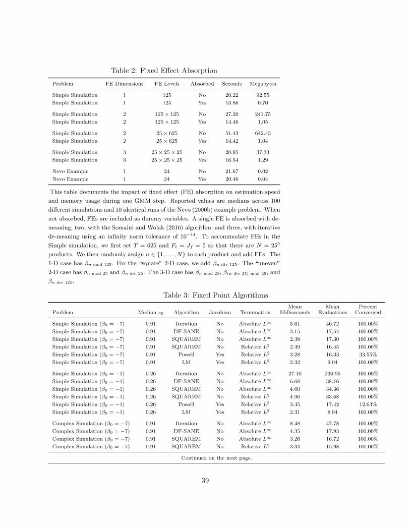
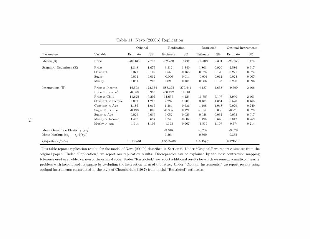
α).10For example Nevo (2001) and Nevo (2000b) includes product fixed effects.

9

[α, ρ, θ2]:11

uijt = δjt(θ1, α) + µijt(θ2) + εijt(ρ).

The primary difference from the nested logit is that the inclusive value term for all products in nest

Jgt now depends on the consumer’s type i:

sjt(δjt, θ2) =

∫exp[(δjt + µijt(θ2))/(1− ρ)]

exp[Iig/(1− ρ)]· exp[Iig]

exp[IVi]f(µijt|θ2) dµit,

Iig(θ1, θ2) = (1− ρ) ln∑j∈Jgt

exp

(δjt + µijt(θ2)

1− ρ

), IVi(θ1, θ2) = ln

1 +G∑g=1

exp Iig

.

(14)

The challenge for estimation is that ln δ·t 7→ln δ·t + lnS·t − ln s·t(δ·t, θ2) is no longer a contraction.

Instead, the contraction must be dampened so that:12

ln δ·t 7→ln δ·t + (1− ρ) [lnS·t − ln s·t(δ·t, θ2)] . (15)

This creates an additional challenge where the rate of convergence for the contraction in (15) can

become arbitrarily slow as ρ→ 1.13 Thus as more consumers substitute within the nest, this model

becomes much harder to estimate. Our simulations will demonstrate that this can be problematic.

As is well known, the relation in (15) has an analytic solution in the absence of random coef-

ficients when µijt = 0 for all (i, j, t). This model reduces to the regular nested logit for which the

following expression was derived in Berry (1994):

ln δjt ≡ lnSjt − lnS0t − ρ lnSj|gt

where Sj|gt is the marketshare of j in its nest g.

3. Algorithmic Improvements in pyblp

In each subsection, we review several methods from the literature (including some of our own

design). While we make many of these methods available as options in pyblp our focus is on

finding best practices which are fastest and most reliable for the widest array of users. Later, we

provide support for these decisions with our Monte Carlo studies.14

11The nesting parameter can also be indexed as ρg so as to vary by group. We support both types of nestingparameters in pyblp.

12See Grigolon and Verboven (2014) for a derivation. The expression in (15) does not precisely match Grigolonand Verboven (2014) because of a typographical error in their final line.

13This can be formalized in terms of the modulus of the contraction mapping or the Lipschitz constant. See Dubeet al. (2012) for more details.

14We chose Python over alternatives such as Matlab, Julia, and R for a number of reasons. Python’s packagemanagement systems are well-established, it has a mature scientific computing ecosystem, and as a general purposelanguage, Python is conducive to the development of larger projects. Scientific computing in all of these high-levellanguages is backed by similar implementations of numerical linear algebra routines, such as BLAS and LAPACK.

10

3.1. Incorporating Many Fixed Effects

There is a long tradition of extending the demand side utility to incorporate product or market

fixed effects. For example Nevo (2001, 2000a) allows for product fixed effects ξj , so that

δjt = [xjt, vjt]β − αpjt + ξj + ∆ξjt.

These can manageably be incorporated as dummy variables (LSDV) in the linear part of the

regression as there are only J = 24 products.

Backus et al. (2018) and Conlon and Rao (2017) allow for product (j) store (or chain) (s)

specific fixed effects djs. Using weekly UPC-store level Nielsen scanner data it is not uncommon

for there to be more that J = 3, 500 products (in both distilled spirits and ready-to-eat cereal).

If one wants to allow for UPC-store fixed effects ξjs this can explode to 100,000 or more fixed

effects. Indeed, in Backus et al. (2018) the authors incorporate more than 50,000 such fixed effects.

Similarly, there are approximately T = 500 weeks t of Nielsen scanner data from 2006-2016. If one

wanted to incorporate store-week fixed effects ξst for only 100 stores this too could reach the order

of 50,000 such fixed effects.

Clearly, the least squares dummy variable (LSDV) approach will not scale with tens or hundreds

of thousands of fixed effects. We might consider the within transformation to remove the fixed

effects, though we can’t directly incorporate both a within transformation and a supply side without

re-writing the problem because of endogenous prices pjt. We show how to re-write the problem in

Appendix A. Define yDjt , ySjt, x

Djt, and xSjt as follows:

yDjt ≡ δjt(θ2) + αpjt = [xjt vjt]β + ξt ≡ xDjtβ + ξjt,

ySjt ≡ pjt − ηjt(θ2) = [xjt wjt]γ + ωt ≡ xSjtγ + ωjt.

Stacking the system across observations yields:[yD

yS

]︸ ︷︷ ︸Y

=

[XD 0

0 XS

]︸ ︷︷ ︸

X

[β

γ

]+

[ξ

ω

]. (16)

After re-arranging terms and re-stacking, this is just a conventional linear IV problem in terms

of (Y,X) where the endogenous parameters have been incorporated into Y . This means that the

within transform can be used to absorb a single dimensional fixed effect.

Consider two dimensions of fixed effects N and T where N T :

yit = yit − yi· − y·t,

xit = xit − xi· − x·t.

See Coleman et al. (2018) for a more detailed comparison of various languages.

11

The simplest approach might be to iteratively demean: remove xi·, update xit, remove x·t, and

repeat this process until xi· = x·t = 0. This method of alternating projections (MAP) can be done

in a single iteration if Cov(x·t, xi·) = 0. However, when the two dimensions of fixed effects are

correlated this can take many iterations and can be quite burdensome.

The LSDV approach handles the burden of correlation but requires constructing the annihilator

matrix to remove all the fixed effects. This approach requires inverting an (N+T )×(N+T ) matrix.

Constructing (and inverting) such a large matrix is often infeasible because of memory requirements.

Several algorithms have been proposed to deal with this problem. The most popular algorithm is

that of Correia (2016), based on the MAP approach of Guimaraes and Portugal (2010), which

iteratively regresses Y on X in order to residualize Y .15

The BLP application is unusual in that we re-run regressions using the XD and XS variables

many times. However, the left hand side variables δjt(θ2) + αpjt and c(θ2) change with each guess

of θ2, which means the entire procedure needs to be repeated for each update of θ2. For two-

dimensional fixed effects, pyblp uses the algorithm of Somaini and Wolak (2016). This has the

advantage that the linear explanatory variables in (XD, XS) can be residualized only once, while

the left hand side variables (which are N × 1 vectors) still need to be residualized for each guess

of θ2. The savings are particularly large when the dimensions of XD or XS are large. For three or

more dimensions of fixed effects, pyblp uses an iterative de-meaning algorithm similar to the one

described above.

3.2. Solving for the Shares

The main challenge of the Nested Fixed Point (NFXP) algorithm is solving the system of market-

shares: Sjt = sjt(δ, θ2). In the NFXP approach, θ2 is treated as fixed, which has the immediate

implication that rather than solving a system of N nonlinear equations and N unknowns in δ, we

solve T systems of Jt equations and Jt unknowns in δ·t. Independent of how we solve each system

of equations, we can solve each market t in parallel.16

Consider a single market t, where we search for the Jt vector δ·t which satisfies

Sjt = sjt(δ·t | θ2) =

∫exp[δjt + µijt]∑k∈Jt exp[δkt + µikt]

f(µit | θ2) dµit (17)

While mathematically there is a unique solution, numerically speaking, it is impossible to choose

a vector δ·t which solves (17) exactly. Instead, we must solve the system of equations to some

tolerance. We express the tolerance in terms of the log difference in shares:

‖lnSjt − ln sjt(δ·t, θ2)‖∞ ≤ εtol. (18)

15This is implemented for the linear IV model in the Stata package ivreghdfe.16This same idea provides the sparsity of share constraints in the MPEC approach of Dube et al. (2012).

12

Users face a tradeoff with regards to the tolerance of the inner loop in (18). If the tolerance is too

loose, the numerical error propagates to the rest of the estimation routine.17 It is also possible to

set a tolerance which is too tight and thus can never be satisfied. This is particularly problematic

when we sum over a large number of elements. We prefer to set εtol ∈ [10−12, 10−14] as the machine

epsilon for 64-bit doubles is generally εmach ∈ [10−16, 10−15].

Jacobian Based Approaches

A direct approach would be to solve the system of Jt equations and Jt unknowns using Newton-type

methods. Consider Newton-Raphson iteration below:18

δh+1·t 7→δh·t − λJ−1

s (δh·t, θ2) · st(δh·t, θ2) (19)

Each Newton-Raphson iteration would require computation of both the Jt vector of marketshares

st(δh·t, θ2), the Jt × Jt Jacobian matrix Js(δ

h·t, θ2) = ∂s·t

∂δ·t(δh·t, θ2), as well as its inverse J−1

s (δh·t).

There are some alternative quasi-Newton methods which solve variants of (19). These variants

generally involve modifying the step-size λ or approximating J−1s (δh·t, θ2) in ways that avoid calcu-

lating the inverse Jacobian at each step. Quasi-Newton methods are often relatively fast when they

work, though they need not converge (they may oscillate, reach a resting point, etc.) and may be

sensitive to starting values.19

Our experience indicates that the Levenberg-Marquardt Algorithm (LMA) is the fastest and

most reliable Jacobian-based solution method.20 LMA minimizes the following least-squares prob-

lem in order to solve the following Jt × Jt system of nonlinear equations:

minδ·t

J∑j=1

[Sj − sj(δ·t, θ2)]2.

The idea is to update our guess of δt to to δt + x where x is a Jt × 1 vector. The LM update is

given by the solution to the following linear system of equations:

[J ′sJs + λdiag(J ′sJs)︸ ︷︷ ︸approximate Hessian

] · x = J ′s[Sj − sj(δ·t, θ2)]. (20)

17Dube et al. (2012) show how error propagates from (18) to the estimates of θ. Lee and Seo (2016) provide a moreprecise characterization of this error when Newton’s method is used.

18In practice it is generally faster to solve the linear system: Js(δh·t, θ2)

[δh+1·t − δh·t

]= −st(δh·t, θ2).

19Though the BLP problem is a non-convex system of nonlinear equations, there are some features which make itamenable to quasi-Newton methods. The marketshare function is a real-analytic function of δ·t; sjt(δ·,t | θ2) is C∞and bounded between (0, 1) and agrees with its Taylor approximation at any δ·t. This guarantees that at least withinsome basin of attraction, quasi-Newton methods will be quadratically convergent. For an example of a quasi-Newtonsolution to Section 3.2, see Houde (2012). The other useful property is that with a strictly positive outside good

share, when all shares sjt < 0.5, the Jacobian Js(δ·t, θ2) is strictly diagonally dominant, which guarantees that it isalways non-singular.

20Specifically we use scipy.optimize.root’s lm option which calls MINPACK’s LM routine (More et al., 1980).

13

This has the advantage that for λ = 0 the algorithm takes a full Gauss-Newton step, while for λ

large it takes a step in the direction of the gradient (gradient-descent). The additional diagonal

term also guarantees the invertibility of approximate Hessian, even when it becomes nearly singular.

As in all iterative solution methods there are two primary costs: the cost per iteration and the

number of iterations until convergence. The cost per iteration is driven primarily by the cost of

computing (rather than inverting) the Jacobian matrix which involves Jt×Jt numerical integrals.21

Fixed Point Approaches

Berry et al. (1995) also propose a fixed-point approach to solve the Jt × Jt system of equations in

(17). They show that the following is a contraction mapping f(δ) = δ:

f : δh+1·t 7→δh·t + lnS·t − ln s·t(δ

h·t, θ2). (21)

This kind of contraction mapping is linearly convergent with a rate of convergence that is propor-

tional to L(θ2)/[1−L(θ2)] where L(θ2) is the Lipschitz constant. Because (21) is a contraction, we

know that L(θ2) < 1. Dube et al. (2012) show that for the BLP contraction the Lipschitz constant

is defined as L(θ2) = maxδ∈∆ ||IJt −∂ log s·t∂δ·t

(δ·t, θ2)||∞.

A smaller Lipschitz constant implies that (21) converges more rapidly. Dube et al. (2012) show

in simulation that all else being equal, a larger outside good share generally implies a smaller

Lipschitz constant.22 Conversely, as the outside good share becomes smaller, the convergence of

the fixed point relationship takes increasingly many steps.

Accelerated Fixed Points

Given a fixed point relationship there may be faster ways to obtain a solution to f(δ) = δ than

direct iteration on the fixed point relation as in (21). There is a large literature on accelera-

tion methods for fixed points. Most of these methods use information from multiple iterations

(δh, δh+1, δh+2, f(δh), f(f(δh))) to approximate Js or its inverse.23

Reynaerts et al. (2012) conduct extensive testing of various fixed point acceleration methods and

find that the SQUAREM algorithm of Varadhan and Roland (2008) works well on the BLP contraction

in (21). The intuition is to form a residual rh which is determined by the change between the current

iteration δh·t and the next iteration f(δh·t), as well as the change in the residual from this iteration

to the next vh to form an estimate of the Jacobian. The residual and the curvature can also be

21A typical entry is∂sjt∂δkt

=∫

[1(j = k)sijt(µit) − sijt(µit)sikt(µit)]f(µit | θ2) dµit. The primary cost arises fromthe numerical integration over heterogeneous types. Even for a large market with Jt = 1, 000 products, inverting a1, 000× 1, 000 matrix is easy relative to J2

t numerical integrals.22A simple but novel derivation. Consider the matrix ∂ log s·t

∂δ·t= IJt − diag−1(s·t)Γ(θ2) where element (j, k) is

1(j = k) − s−1jt

∫sijt(µit)sikt(µit)f(µit | θ2) dµit. This implies that L(θ2) = maxδ[maxj s

−1jt

∑k |Γjk(δ·t, θ2)|]. A

rough approximation to the term inside the square braces is maxj∑k |skt| · |ρ(sijt, sikt)| < 1− s0t.

23Many of these algorithms are special cases of Anderson Mixing.

14

used to construct a step-size αh. The exact algorithm is described below:24

δh+1·t 7→δh·t − 2αhrh + (αh)2vh,

αh =(vh)′rh

(vh)′vh, rh = f(δh·t)− δh·t, vh = f(f(δh·t))− 2f(δh·t) + δh·t.

(22)

In general the SQUAREM method is 4 to 8 times as fast as direct iteration on the BLP contraction in

(21). The idea is to take roughly the same number of steps as Newton-Raphson iteration, but to

reduce the cost of steps by avoiding calculating the Jacobian directly. In fact, all of the terms in

(22) are computed as a matter of course, because these are just iterations of xh and f(xh). Unlike

direct iteration on (21), there is technically no convergence guarantee as the iteration on (22) is no

longer a contraction.

The are alternative acceleration methods in addition to SQUAREM. Reynaerts et al. (2012) also

consider DF-SANE which takes on the form δh+1·t 7→δh·t − αhf(δh·t) with a different choice of the

step-size αh. They find performance is similar to SQUAREM though it can be slightly slower and less

robust. Consistent with Reynaerts et al. (2012), we find the SQUAREM to be the fastest and most

reliable fixed-point approach. We find that the Jacobian-based Levenberg-Marquardt approach

gives similar reliability and (slightly better) performance.

3.3. Optimization

Optimization of the GMM objective function for the BLP problem can be challenging. The BLP

problem itself in (9) represents a non-convex optimization problem,25 so the Hessian need not

be positive semidefinite at all values of θ2. In practice this means that no optimization routine

is guaranteed to find a global minimum in a fixed amount of time. This critique applies both

to derivative-based quasi-Newton approaches and to simplex-based Nelder-Mead type approaches.

Well-known recommendations involve considering a number of different starting values and opti-

mization routines, verifying that θ satisfies both the first order conditions (the gradient is within

a tolerance of zero) and second order conditions (the Hessian matrix has all positive eigenvalues).

Both of these are reported by default in pyblp.

The optimization interface to pyblp is generic in the sense that any optimizer which can be

implemented as a Python function should work fine.26 Though non-derivative based routines such

as Nelder-Mead have been frequently used in previous papers, they are not recommended.27 Indeed,

24pyblp includes a Python port of the SQUAREM package from R.25Absent unobserved heterogeneity or random coefficients the problem is globally convex.26To illustrate this, in the documentation we give an example of such a “custom” routine where we construct

a simple brute force solver that searches over a grid of parameter values. This flexibility should allow users toexperiment with routines without much difficulty or “upgrade” if better routines are developed.

27Both Dube et al. (2012) and Knittel and Metaxoglou (2014) find that derivative-based routines outperform thesimplex-based Nelder-Mead routine both in terms of speed and reliability. Our own tests concur with this prioropinion.

15

the most important aspect of pyblp optimization is that it calculates the analytic gradient for any

user-provided model, including models which incorporate both supply and demand moments or

fixed effects.28 Analytic gradients provide both a major speedup in computational time, while also

generally improving the chances that the algorithm converges to a valid minimum.

The pyblp package uses optimization routines implemented in the open-source SciPy library

and also interfaces with commercial routines such as Artleys Knitro. The Knitro software in-

corporates four different gradient-based search routines, and has been recommended for the BLP

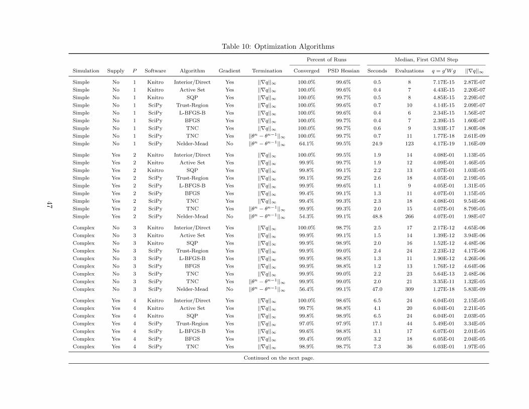
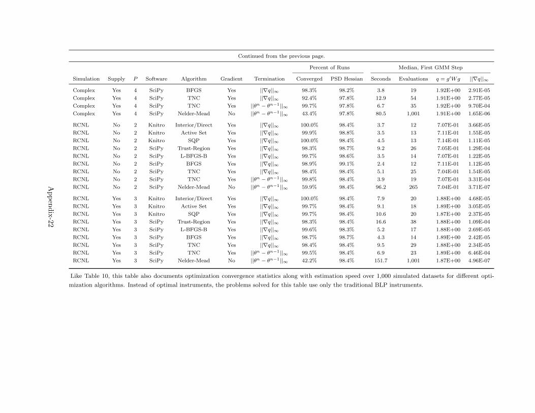
problem previously by Dube et al. (2012). Table 10 lists nine different optimization routines cur-

rently supported by pyblp. Some optimization routines also allow the user to input constraints on

parameters, these can speed up estimation or prevent the optimization routine from considering

“unreasonable” values. An important example are box constraints on the parameter space, where

we restrict components of θ2 denoted θ` to θ` ∈ [θ`, θ`]. Some typical constraints are that demand

slopes down and that random coefficients have positive but bounded variances. This is particularly

helpful because large values for random coefficients can generate numerical issues which we discuss

below.

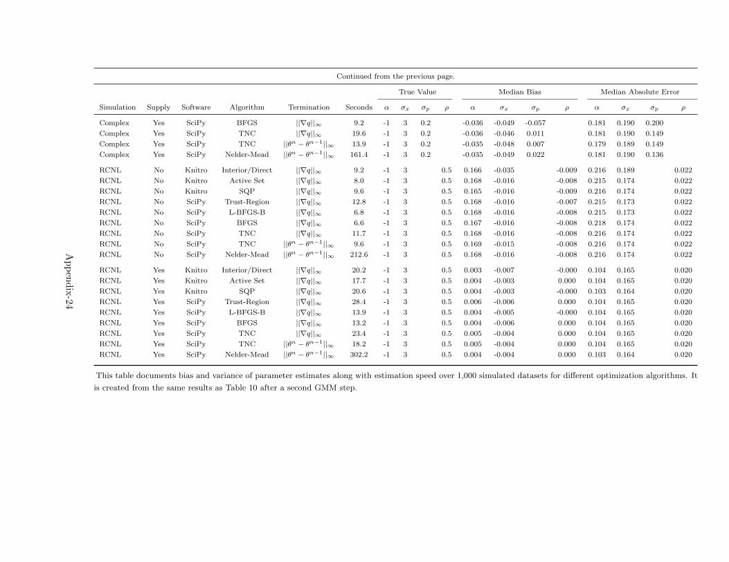
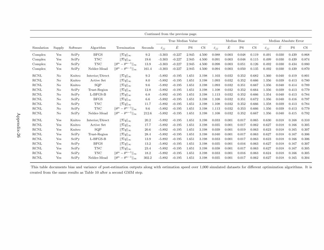
Consistent with the prior literature, we recommend trying multiple different optimizers and

starting values to check for agreement; our simulations indicate that when properly configured,

most optimizers arrive at the same parameter estimates. Our recommendation is that researchers

try Knitro’s Interior/Direct algorithm first if available, and then try a BFGS-based routine, ideally

with constraints on the parameter space such as L-BFGS-B.29

3.4. Numerical Issues and Tricks

There are several numerical challenges posed by the BLP problem, most of which are related to the

exponentiated indirect utilities and the logit denominator:∑

j exp[δjt+µijt]. If some values in this

summation are on the order of exp(−5) ≈ 0.0067 and others are exp(30) > 1013, their sum may

be rounded because the effective precision for most 64-bit doubles is around 15 significant digits.

This loss of precision arises when taking summations of many numbers with different scales, and

depending on the situation, may or may not be problematic. A related problem is overflow, which

is likely to arise when attempting to compute large values such as exp(300). This can mean that

sjt(δ·t, θ2)→ 1 while skt(δ·t, θ2)→ 0 for k 6= j, and leads optimization routines to fail.30

There are a number of solutions to these problems. One solution is to avoid large values in the

argument of exp(·) by limiting the magnitudes of random coefficients through the box constraints

described above. Another simple solution involves working market by market and avoiding very

large summations. One additional method would be to use a summation algorithm that attempts to

28We could not find any examples of simultaneous estimation of supply and demand with analytic gradients inthe literature. A likely explanation is that the derivatives of the markup term ηjt(θ2) are quite complicated. SeeAppendix B for a derivation.

29The main disadvantage of Knitro is that it is not freely available—it must be purchased and installed by end-users.30In this case sjt(δ·t, θ2) = sjt cannot be solved for δ·t, thus the inversion for the mean utilities fails.

16

preserve precision such as Kahan Summation.31 This is substantially slower and is not implemented

by default. As suggested in Skrainka (2012b), yet another approach is to use extended precision

arithmetic. Again, we found this to be substantially slower without improving our statistical

performance.32

Another way to guarantee overflow safety is to use a protected version of the log-sum-exp (LSE)

function: LSE(x1, . . . , xK) = log∑

k expxk = a + log∑

k exp(xk − a). By choosing a = maxk xk,

use of this function helps ensure overflow safety when evaluating the multinomial logit function.

This is a well known trick from the applied mathematics and machine-learning literatures, but

there does not appear to be evidence of it in the literature on BLP models. This is implemented

by default, as the additional computational cost appears to be trivial.

Implementations of the BLP method have used a number of “tricks” specific to certain software

packages (such as MATLAB) in order to speed up the algorithm. One well-known trick involves

working with exp[δjt] in place of δjt in the contraction mapping to avoid transcendental functions

like exp(·). This has little benefit on modern architectures as transcendentals are highly optimized

and exp(·) of a billion numbers takes less than one millionth of a second. Another trick is using

δ·t from a previous guess of θ2 as a starting value. The SQUAREM and LM algorithms we suggest

for solving the system of equations are relatively insensitive to starting values, so these sorts of

speedups are not particularly useful. A MATLAB specific “vectorization” speedup used in Nevo

(2000b) and Knittel and Metaxoglou (2014) is to stack all markets together and then construct

cumulative sums of exp[δjt + µijt]. We find that this is approach is dominated by parallelization

across markets T ; furthermore, this approach will results in a loss of precision as T → ∞. We

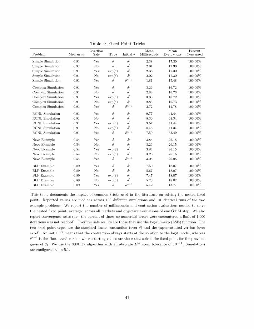
provide some analysis of these tricks in Table 4.

3.5. Heterogeneity and Integration

An important aspect of the BLP model is that it incorporates heterogeneity via random coefficients.

The challenge is that the integration in (3) needs to be performed numerically:

sjt(δt, θ2) =

∫exp[δjt + µijt]∑k∈Jt exp[δkt + µikt]

f(µit|θ2)dµit ≈It∑i=1

wiexp[δjt + µijt(νit)]∑k∈Jt exp[δkt + µikt(νit)]︸ ︷︷ ︸

sijt(µit(θ2))

. (23)

The most common approach is Monte Carlo integration where random draws are taken from some

candidate distribution νit ∼ f(νit|θ2) and then used to calculate µijt(νit, θ2). We can then take a

weighted sum of individuals sjt(δt, θ2) =∑It

i=1wisijt(δt, µit(θ2)). The main advantage of Monte-

31In Python this is implemented as math.fsum.32We are a bit vague on exactly what “extended precision” means because the NumPy implementation of

numpy.longdouble varies across different architectures. On most Unix platforms, it is implemented with a 128-bit long double. For problems very different from our Monte Carlo designs with very small shares, or for problemswith very large numbers of products, additional precision might still be valuable.

17

Carlo integration (actually pseudo-Monte Carlo integration) is that it avoids the curse of dimension-

ality. While the accuracy for low dimensional integrals increases slowly in the number of points of

approximation, the accuracy does not decline quickly as one increases the dimension of integration.

The second approach is the so-called Gaussian quadrature approach. Here the integrand is

approximated with a polynomial and then integrated exactly as polynomial integration is trivial.

In practice this is far simpler as it still amounts to a weighted sum in (23) over a particular choice

of (νi, wi). The main choice the user makes is the polynomial order of the rule. In effect the user

chooses the order of the polynomial used to approximate the integrand. As the order grows, more

nodes are required but the accuracy of the approximation improves.

Gaussian quadrature works best when certain conditions are met: that the integrand is bounded

and continuously differentiable. Thankfully, the logit kernel in (23) is always bounded on (0, 1) and

is infinitely continuously differentiable. This lends itself to quadrature-type approaches. There

are a number of different flavors of quadrature rules designed to best approximate integrals under

different weighting schemes. The Gauss-Hermite family of rules work best when f(µit) ∝ exp[−µ2it],

which (with a change of variables) includes integrals over a normal density. Gauss-Kronod rules

offer an alternative where for a given level of polynomial accuracy p, they reuse the set of nodes

from the p − 1 polynomial accuracy integration rule. This allows for adaptive accuracy without

wasting calculations; when the error from numerical integration is large the the polynomial degree

can be expanded. Both the advantage and disadvantage of Gaussian quadrature rules is that they

do a better job covering the “tail” of the probability distribution. While this increases the accuracy

of the approximation, it can also lead to very large values which create overflow issues.33 We prefer

to use quadrature rules, and to be careful of potential overflow/underflow issues when computing

shares.

The Gaussian quadrature rules apply only to a single dimension. One way to estimate higher

dimensional integrals is to construct the product of single dimensional integrals. The disadvantage

of product rules is that if one needs It points to approximate the integral in dimension one, then

one needs Idt points to approximate the integral in dimension d. This is the so-called curse of

dimensionality.

The curse of dimensionality is a well-known problem in numerical analysis and several off-the-

shelf solutions exist. There are several clever algorithms for improving upon the product rule for

higher dimensional integration. Judd and Skrainka (2011) explore monomial cubature rules while

Heiss and Winschel (2008) use sparse grid methods to selectively eliminate nodes from the product

rules. One disadvantage of these methods is that they often involve weights which are negative (i.e.,

wi < 0), which can create problems when trying to decompose the distribution of heterogeneity

(particularly for counterfactuals).

Though pyblp allows for flexible (user-supplied) distributions of random coefficients, by far

33Essentially for some simulated individual i we have that sijt → 1 and sikt → 0. This problem has been previouslydocumented by Judd and Skrainka (2011) and Skrainka (2012b).

18

the most commonly employed choices in the literature are the independent normal and correlated

normal distributions for f(νi | θ2). Here pyblp provides some specialized routines to handle these

integrals with limited user intervention. There are number of different methods one can use to

generate (wi, νi) for the (correlated) normal case:

1. monte carlo: Draw νi` from the standard normal distribution for each dimension of hetero-

geneity `. Set wi = 1/It where It is the number of simulated “individuals”.

2. product: Construct the Gauss-Hermite quadrature rule (νi, wi) for a single dimension and

build a product rule to obtain a set of weights and nodes in a higher dimension d.

3. nested product: Construct (νi, wi) using a product rule in dimension d but beginning with

the basis of Gauss-Kronrod instead of Gauss-Hermite.

4. grid: Construct (νi, wi) using a sparse grid rule of Heiss and Winschel (2008) for dimension

d with the Gauss-Hermite rule as an initial basis.

5. nested grid: Construct (νi, wi) using a sparse grid rule in dimension d but beginning with

the basis of Gauss-Kronrod instead of Gauss-Hermite.

6. Construct (νi, wi) from user-provided data which allows for pseudo-Monte Carlo methods

such as Halton draws or Sobol sequences.

In general, the best practice in low dimensions is probably to use product rules to a relatively high

degree of polynomial accuracy. In higher dimensions, sparse grids appear to scale the best both in

our own Monte Carlo studies and in those of Judd and Skrainka (2011) and Heiss and Winschel

(2008).

3.6. Solving for Pricing Equilibria

Many counterfactuals of BLP-type problems involve perturbing either the market structure, marginal

costs, or both, and solving for counterfactual equilibrium prices. Being able to solve for equilib-

rium prices quickly and accurately is also crucial to generating the optimal instruments in the next

section. The Bertrand-Nash first order conditions are defined by (5) for each market t:

p = c + ∆(p, O)−1s(p)︸ ︷︷ ︸η(p,O)

During estimation, in order to recover marginal costs, one need only invert the Jt × Jt matrix

∆(p, O). Solving for counterfactual pricing equilibria is more difficult as now we must solve the

Jt×Jt nonlinear system of equations, often after replacing the ownership matrix with a post-merger

counterpart, O → Opost:

p = c + ηpost(p, Opost). (24)

19

In general, solving this problem is hard as it represents a non-convex nonlinear system of equa-

tions, where one must simulate in order to compute η(p, Opost) and its derivatives.34 Once one

incorporates both multi-product firms and arbitrary coefficients into the problem, both existence

and uniqueness of an equilibrium become challenging to establish.35

One approach might be to solve the system using Newton’s method, which requires calculating

the Jt × Jt Jacobian ∂η(p)∂p . We provide (possibly novel) analytic expressions for this Jacobian in

Appendix B.36 The expression for the Jacobian involves the Hessian matrix of demand ∂2sk∂p2j

as well

as tensor products, and can be computationally challenging.37

The second, and perhaps most common approach in the literature is treating (24) as a fixed

point and iterating on p 7→c + ηpost(p, Opost).38 The problem is that while a fixed point of (24)

may represent the Bertrand-Nash equilibrium of (7), it is not necessarily a contraction. In fact, as

part of Monte Carlo experiments conducted in Armstrong (2016), the author finds that iterating

on (24) does not always lead to a solution and at least some fraction of the time leads to cycles.

We were able to replicate this finding for similarly constructed Monte Carlo experiments between

1-5% of the time. Were this relation to be a contraction, we should always be able to iterate on

p 7→c + ηpost(p, Opost) until we reached the solution.

Our preferred approach borrows from the engineering literature and follows Morrow and Skerlos

(2011). This approach does not appear to be well known in the Industrial Organization literature,

but in our experiments appears to be highly effective. They reformulate the solution to (5) by

breaking up the matrix of demand derivatives into two parts: a Jt × Jt diagonal matrix Λ, and a

Jt × Jt dense matrix Γ:

∂s

∂p(p) = Λ(p)− Γ(p),

Λjj =

∫αisijt(µit)f(µit | θ2) dµit,

Γjk =

∫αisijt(µit)sikt(µit)f(µit | θ2) dµit,

(25)

34The first Monte Carlo studies which evaluate price and quantity equilibria as part of the data generating processare likely Armstrong (2016), Skrainka (2012a) and Conlon (2017).

35Caplin and Nalebuff (1991) and Gallego et al. (2006) have results which apply to single product firms and linearin price utility under logit demands. Konovalov and Sandor (2010) generalizes these to logit demands with linear inprice utility and multi-product firms. With the addition of random coefficients, it is possible that the resulting modelwill violate the quasi-concavity of the profit function that these results require. Morrow and Skerlos (2010) avoidsome of these restrictions but place other restrictions on indirect utilities. Existence and uniqueness are beyond thescope of this paper—we instead focus on calculating solutions to the system of first order conditions, assuming suchsolutions exist.

36For example, Knittel and Metaxoglou (2014) do not update s(p) and thus avoid fully solving the system ofequations.

37An alternative might be to try a Newton-type approach without providing analytic formulas for the Jacobian. Thisseems slow and ill-advised as there are Jt markups each with Jt derivatives and each derivative involves integrationin order to compute both Ω(p) and s(p).

38The “folklore” solution is to dampen this expression and consider p 7→ρ · p + (1− ρ) ·[c + ηpost(p, Opost)

]. This

tends to be slower and more reliable, though we cannot find any theoretical justification for convergence.

20

where αi =∂uijt∂pjt

, the marginal (dis)-utility of price. Morrow and Skerlos (2011) then reformulate

the problem as different fixed point that is specific to mixed logit demands:39

p 7→c + ζ(p), ζ(p) = Λ(p)−1(Opost Γ(p))(p− c)− Λ(p)−1s(p). (26)

The fixed point in (26) is entirely different from that in (24) and coincides only at resting points.

Consistent with results reported in Morrow and Skerlos (2011), we find that (26) is around 3-12

times faster than Newton-type approaches and reliably finds an equilibrium.40

Perhaps most consequentially, the ability to solve for a pricing equilibrium rapidly and reliably

makes it possible to generate the Amemiya (1977) or Chamberlain (1987) feasible approximation

to the optimal instruments.

4. Supply and Demand: Optimal Instruments and Overidentifying Restrictions

This section focuses on joint estimation of supply and demand in order to clarify the precise role

of overidentifying restrictions. Absent information on firm conduct or the precise functional form

for marginal costs, many researchers estimate a demand side only.

As a way to improve performance, we can construct approximations to the optimal instruments

in the spirit of Amemiya (1977) or Chamberlain (1987). Approximations to the optimal instruments

were featured in both Berry et al. (1995) and Berry et al. (1999) but are not commonly employed in

many subsequent studies using the BLP approach in part because they are challenging to construct.

Reynaert and Verboven (2014) show approximations to the optimal instruments can improve the

econometric performance of the estimator, particularly with respect to the θ2 parameters. The form

we derive is somewhat different from their expression, and incorporates both supply and demand.

While the procedure itself is quite involved, the good news is that does not require much in the

way of user input, and is fully implemented by the pyblp software.

For the GMM problem, Chamberlain (1987) tells us that the optimal instruments are related

to the expected Jacobian of the moment conditions where the expectation is taken conditional only

on the exogenous regressors zt. We can write this expectation for each product j and market t

as E[Dj(zt)Ω−1jt | zt]. We use the word “approximation” because the aforementioned expectation

39This resembles a well known “folklore” solution to the pricing problem, which is to rescale each equation by itsown share sjt (see Skrainka, 2012a). For the plain logit, Λ−1

jj = 1/(αsj).40In pyblp, iteration is terminated with the numerical simultaneous stationarity condition of Morrow and Skerlos

(2011) is satisfied: ||Λ(p)(p − c − ζ(p))|| < ε, where ε is a small number and the left hand side is firms’ first orderconditions.

21

lacks a closed form. We derive the components of the approximation below:41

Dj ≡

∂ξj∂β

∂ωj∂β

∂ξj∂α

∂ωj∂α

∂ξj

∂θ2

∂ωj

∂θ2∂ξj∂γ

∂ωj∂γ

︸ ︷︷ ︸

(K1+K2+K3)×2

=

−xj 0

−vj 0∂ξj∂α

∂ωj∂α

∂ξj

∂θ2

∂ωj

∂θ2

0 −xj0 −wj

, Ω ≡

[σ2ξ σξω

σξω σ2ω

]︸ ︷︷ ︸

2×2

. (27)

A little calculation shows that for each market t and each observation j,

DjΩ−1 =

1

σ2ξσ

2ω − σ2

ξω

×

−σ2ωxj σξωxj

−σ2ωvj σξωvj

σ2ω∂ξj∂α − σξω

∂ωj∂α σ2

ξ∂ωj∂α − σξω

∂ξj∂α

σ2ω∂ξj

∂θ2− σξω

∂ωj

∂θ2σ2ξ∂ωj

∂θ2− σξω

∂ξj

∂θ2

σξωxj −σ2ξxj

σξωwj −σ2ξwj

. (28)

Clearly rows 1 and 5 are co-linear. Let Θ be a conformable matrix of zeros and ones such that

(DjΩ−1)Θ =

1

σ2ξσ

2ω − σ2

ξω

×

−σ2ωxjt 0

−σ2ωvj σξωvj

σ2ω∂ξj∂α − σξω

∂ωj∂α σ2

ξ∂ωj∂α − σξω

∂ξj∂α

σ2ω∂ξj

∂θ2− σξω

∂ωj

∂θ2σ2ξ∂ωj

∂θ2− σξω

∂ξj

∂θ2

0 −σ2ξxj

σξωwj −σ2ξwj

. (29)

We can partition our instrument set by column into “demand” and “supply” instruments:

zDj ≡ E[(DjΩ−1jt Θ)·1 | z]︸ ︷︷ ︸

K1+K2+(K3−Kx)

, zSj ≡ E[(DjΩ−1jt Θ)·2 | z]︸ ︷︷ ︸

K2+K3+(K1−Kx)

. (30)

In (30), we have K −Kx (where Kx denotes the dimension of common exogenous parameters xjt)

instruments for both supply zSj and demand zDj , though it is evident from (28) that the instruments

for the endogenous parameters are not the same.42 The approximate optimal instruments from the

endogenous parameters are nonlinear functions of the data, while the remaining optimal instru-

41Implicitly we assume that (ξjt, ωjt) are jointly IID so that Ωjt = Ω. This is merely a matter of convenientnotation, as the extention to heteroskedastic or clustered covariances are straightforward.

42This is true except for the knife-edge case where∂ξj∂θ`

/∂ωj∂θ`∝ σ2

ξ+σξσ

σ2ω+σξσ

. In fact, (30) highlights that the set of

instruments ZD and ZS should never be the same because of the different excluded variables.

22

ments from the linear portions of demand and supply are simply exogenous regressors re-scaled by

covariances.

Notice that when we include simultaneous supply and demand moments we have overidentifying

restrictions. As shown in (30), we have 2 × (K −Kx) restrictions and K parameters. This gives

us K − 2Kx overidentifying restrictions. The first set of K2 overidentifying restrictions comes from

the fact that in (28) we have two restrictions for each of the endogenous (nonlinear) parameters

[α, θ2]. These are cross-equation restrictions that arise from simultaneous estimation of supply and

demand.

The other two sets of overidentifying restrictions arise from exclusion restrictions, which are

made explicit in (30), where wjt and vjt show up in one equation but not the other. There are

K3−Kx overidentifying restrictions from cost shifters wjt which are excluded from demand. There

are K1 −Kx demand shifters vjt which are excluded from supply.

Remark 1

Our version of the optimal instruments makes explicit the exclusion restrictions in the BLP model.

Both the supply and demand moments are used in order to pin down the endogenous parameters θ2

(including the price parameter α). The role of the exogenous cost-shifters wjt is now explicit: they

provide overidentifying restrictions for demand which can be used to pin down α and θ2. Likewise

the role of the exogenous demand-shifters vjt is also made explicit: they provide overidentifying

restrictions for supply which can be used to pin down θ2 as well as the markup term ηjt(θ2), and

hence firm conduct.

Perhaps most importantly, this tells us precisely where to find exclusion restrictions: something

that enters the other equation. The idea of using demand shifters as overidentifying restrictions to

identify conduct has a long history in industrial organization going back to Bresnahan (1982), and

was treated non-parametrically in Berry and Haile (2014). In related work, Backus et al. (2018)

show how to use (29) to test for firm conduct.

Remark 2

It is worth pointing out that our derivation of the optimal instruments appears to vary from

derivations in the prior literature. Some of the prior literature using optimal instruments for BLP

type problems suggests the resulting problem is just identified rather than over identified. Reynaert

and Verboven (2014) appear to construct their version of optimal instruments by summing across

the rows of (28) and excluding either the first or third row.43 This gives them K = K1 +K2 +K3

instruments and K unknowns so that the model is just identified. However, because they stack

(ξ, ω) they effectively have 2×N rather than N observations. Conceptually, one way to view their

formulation is that it imposes E[ξ′jtzjt]+E[ω′jtzjt] = 0 rather than separately imposing E[ξ′jtzjt] = 0

43We should caveat that Reynaert and Verboven (2014) do not consider joint supply and demand as their mainspecification.

23

and E[ω′jtzjt] = 0.

Remark 3

If one assumes that σξω = 0 or that the supply and demand shocks are uncorrelated, then the

expression in (28) clearly shows that the optimal instruments for demand no longer depend on the

supply Jacobian∂ξj∂θ2

and likewise that the optimal instruments for supply no longer depend on the

demand Jacobian∂ωj∂θ2

.44 We still have overidentifying restrictions in this case as both supply and

demand moments provide information on the nonlinear parameters. We caution that there is no a

priori reason to believe that supply and demand unobservables are uncorrelated with one another.

Constructing Feasible Instruments

The main challenge with implementing the optimal instruments is that the expectations of the

Jacobian terms E[∂ξj∂θ2

,∂ωj∂θ2| z] are not directly measured. The most obvious example is that

∂ξj∂α = pj , but pj is endogenous, so we must replace it with some estimate of E[pj | z]. Here is what

Berry et al. (1995) say about optimal instruments:

Unfortunately Dj(z) is typically very difficult, if not impossible, to compute. To calculate

Dj(z) we would have to calculate the pricing equilibrium for different (ξj , ωj) sequences,

take derivatives at the equilibrium prices, and then integrate out over the distribution

of such sequences. In addition, this would require an assumption that chooses among

multiple equilibria when they exist, and either additional assumptions on the joint dis-

tribution of (ξ, ω), or a method for estimating that distribution.

The appendix of the NBER working paper version of Berry et al. (1999) is even less positive:

Calculating a good estimate of E[p | z] then requires (i) knowing or estimating the

density of the unobservables and (ii) solving at some initial guess for θ the fixed point

that defines equilibrium prices for each (ξ, ω) and then integrating this implicit function

with respect to the density of the unknown parameters. This process is too complicated

to be practical.

In their main specification, Reynaert and Verboven (2014) suggest computing the approxima-

tion to the optimal instruments under an additional assumption of perfect competition, so that

E[pjt | z] = E[cjt | z] = [xjt wjt]γ + ωjt. This avoids solving for equilibrium prices (and implicit

functions). When they do consider imperfect competition, they construct E[pjt | zt] by regressing

the endogenous variable on a series of exogenous regressors (essentially a “first stage” regression).

We follow the possibly more accurate but costly recipe proposed by Berry et al. (1999) and

show that with other computational advances in pyblp it is feasible to implement. For each market

t we can:44In this case the optimal weighting matrix would also have a block diagonal structure with separate blocks for

demand and supply moments. The zero covariance restriction is the identification argument in MacKay and Miller(2018).

24

1. Obtain an initial estimate θ = [β, α, θ2, γ].

2. Obtain an initial estimate of Ω−1 by computing covariances of (ξ, ω).

3. Draw the Jt × 2 matrix of structural errors (ξ∗t , ω∗t ) according to one of the below options.

4. Compute ySjt = cjt = [xjt wjt]γ + ω∗jt and the exogenous portion of utility yDjt = xjtβ + ξ∗jt.

5. Use (yDjt , ySjt, α, xt, wt) to solve for equilibrium prices and quantities (pt, st) with the ζ-markup

approach in Section 3.6. Note that this does not include any endogenous quantities.

6. Treating (pt, st, xt, wt) as data, solve for ξ = ξ(pt, st, xt, wt, α, θ2) and ωt = ω(pt, st, xt, wt, α, θ2)

following Section 2.1.

7. Construct the Jacobian terms∂ξj∂θ2

(ξ∗t , ω∗t ),

∂ωj∂θ2

(ξ∗t , ω∗t ), and Dj(ξ

∗t , ω

∗t ) using the analytic for-

mulas in Appendix B.

8. Average Dj(ξ∗t , ω

∗t ) over several draws of (ξ∗t , ω

∗t ) to construct an estimate of E[Dj | zt].

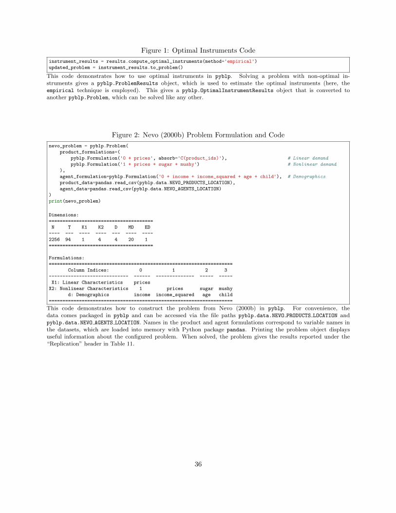
There are three options for generating (ξ∗t , ω∗t ) suggested by Berry et al. (1999) and pyblp makes

all three available:

(a) approximate: Replace (ξ∗t , ω∗t ) with their expectation: (E[ξt], E[ωt]) = (0, 0). This is what

Berry et al. (1999) do.

(b) asymptotic: Estimate an asymptotic normal distribution for (ξjt, ωjt) ∼ N(0, Ω) and then

draw (ξ∗t , ω∗t ) from that distribution.

(c) empirical: Draw (ξ∗t , ω∗t ) from the joint empirical distribution of (ξjt, ωjt).

In general, asymptotic and empirical are not believed to be computationally feasible, particularly

when there are large numbers of draws for (ξ∗t , ω∗t ). The costly step is Item 5 above which involves

solving for a new equilibrium (pt, st) for each set of draws. These improved optimal instruments are

only really feasible because of the advances in Section 3.6, which drastically reduce the amount of

time it takes to solve for equilibria. For relatively large problems, constructing optimal instruments

may take several minutes. For smaller problems such as Berry et al. (1995) or Nevo (2000b) it takes

only several seconds. Our simulations indicate that approximate performs as well as the more

expensive asymptotic or empirical formulations. Updating results with optimal instruments in

pyblp requires only the two lines of code in Figure 1.

Demand Side Only

Most empirical applications of the BLP approach do not include a supply side, but estimate demand

alone. This has some advantages and some disadvantages. One important implication is that we

lose the cross-equation overidentifying restrictions. The absence of the supply side should make it

25

harder to pin down θ2 parameters in particular. However, we still retain the K3 − Kx exclusion

restrictions for demand from the cost-shifters wjt. Absent these cost-shifters and without additional

restrictions, the endogenous price parameter is not identified. As we show in our simulation results,

a correctly specified supply side and the optimal instruments together appear to be quite powerful

in pinning down parameters, even when other instruments appear weak.

Absent the supply side, we no longer have a model for marginal costs and cannot solve for

equilibrium (pt, st). Instead, the user can supply a vector of expected prices E[pt | zDt ] or allow

pyblp to construct the vector with a first-stage regression similar to Reynaert and Verboven (2014).

The value of the (approximate) optimal IV now depends on how well price is explained by the

exogenous instruments (xjt, wjt).

Remark 4

In our Monte Carlo exercise, we find a substantial additional benefit when incorporating both a

supply-side as well as the approximation to the optimal IV. This arises from the difference between

the nonlinear form of E[pt|zDt ] under the approximation to the optimal IV, and the linear projection

of pt onto zDt .

The main advantage of omitting the supply side is that including a mis-specified supply side may

be worse than no supply side at all. The most controversial aspect of the supply side is often the

conduct assumption used to recover the markup ηjt(θ2), which may not be known to the research

prior to estimation. The good news is that testing the validity of the supply side moments amounts

to a test of over-identifying restrictions. The simplest test involves estimating the full model with

supply and demand to obtain θ, re-estimating the model using only demand moments to obtain

qD(θD), and then comparing GMM objectives in a Hausman manner (see Newey, 1985):

LR = Nq(θ)−NqD(θD) ∼ χ2K−Kx . (31)

There are of course alternatives based on the LM (Score) and Wald tests.

5. Monte Carlo Experiments

Here we provide some Monte Carlo experiments to illustrate some of the best practices laid out in

Section 3 and Section 4.45

5.1. Monte Carlo Configuration

Our simulation configurations are loosely based on those of Armstrong (2016). The most important

is that we solve for equilibrium prices and shares. For each configuration, we construct and solve

45We solve our simulations with an Intel Xeon E5-2697 v2 processor operating at 2.70 GHz and DDR3 DIMMoperating at 1,866 MHz.

26

1,000 different synthetic datasets. There are F = 5 firms, and each produces a number of products

chosen randomly from Jf ∈ 2, 5, 10. There are T = 20 markets, and in each market, the number of

firms is chosen randomly from Ft ∈ F−2, F−1, F = 3, 4, 5. This procedure generates variation

in the number of firms and products across markets which can be helpful for identification. Sample

sizes are generally within N ∈ [200, 600].

We draw the structural error terms (ξjt, ωjt) from a mean-zero bivariate normal distribution

with σ2ξ = σ2

ω = 0.2 and σξω = 0.1. Linear demand characteristics are X1 = [1, x, p] and supply

characteristics are X3 = [1, x, w]. The one nonlinear characteristic is X2 = x and heterogeneity is

parameterized by µijt = σxxjtνi where we draw νi from the standard normal distribution for 1,000

different individuals in each market. We draw the two exogenous characteristics (xjt, wjt) from the

standard uniform distribution and compute the endogenous (pjt, sjt) with the ζ-markup approach

of Section 3.6.

Demand-side parameters are [β0, β1, α]′ = [−7, 6,−1]′ and σx = 3. Other linear parameters were

chosen to generate realistic outside shares generally within s0t ∈ [0.8, 0.9]. Supply-side parameters

[γ0, γ1, γ2]′ = [2, 1, 0.2]′ enter into a linear functional form for marginal costs: c = X3γ + ω.

In our different Monte Carlo experiments we modify this baseline problem in a number of ways.

In most experiments, we consider three variants:

(a) Simple is the baseline problem described above.

(b) Complex adds a random coefficient on price: X2 = [x, p] and σp = 0.2.

(c) RCNL adds a nesting parameter ρ = 0.5. Each of the Jf products produced by a firm is

randomly assigned to one of two nesting groups.

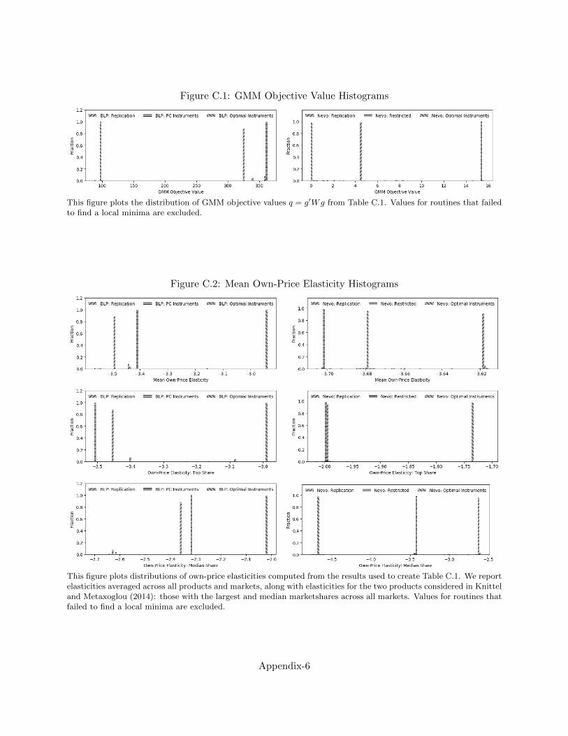
Two broad classes of models are estimated: demand-only models, which are estimated with single

equation GMM, and models that also include the supply side, which are estimated with multiple

equation GMM.

Instruments are constructed in two stages. The initial instruments consist of all exogenous

regressors and BLP instruments (characteristics of other products). We begin with the classic

“sums of characteristics” version, and then move to improved versions. For each product j we sum

the product characteristics for other products controlled by the same firm f and those controlled

by competing firms within the same market t:

ZD,BLPjt = ZS,BLP

jt =

1, xjt, wjt,∑

k∈Jft\j

1,∑k/∈Jft

1,∑

k∈Jft\j

xkt,∑k/∈Jft

xkt

. (32)

For some specifications we include the differentiation IV of Gandhi and Houde (2017). These are

a variant on the BLP instruments as they represent a different function of own and rival product

characteristics. Pooling products across all markets, for each pair of products (j, k), we construct

27

the difference djk = xk − xj of the exogenous regressor and then form two types of differentiation

IV, which are

ZD,Localjt = ZS,Localjt =

1, xjt, wjt,∑

k∈Jft\j

1(|djk| < σd),∑k/∈Jft

1(|djk| < σd),

ZD,Quadjt = ZS,Quad

jt =

1, xjt, wjt,∑

k∈Jft\j

d2jk,∑k/∈Jft

d2jk

.

(33)

The differentiation IV come in two flavors: Local and Quadratic. In both cases, the differentiation

IV are constructed by computing the distance in characteristic space between products j and k.

The Local measure counts the number of products within a standard deviation of product j, while

the Quadratic measure sums up the aggregate distance between j and other products.

Following Gandhi and Houde (2017), for the Complex simulation where there is a random

coefficient on price, we construct an additional instrument using fitted values from a regression

of endogenous prices onto all exogenous variables (including the constructed instruments above).

Further following the suggestions of Berry (1994) or Gandhi and Houde (2017) for discrete variables,

for the RCNL simulation, we also include counts of products within the same nest.

Our approximation to the optimal instruments are constructed in three different variants follow-

ing Section 4. When a supply side is included, the vector of expected prices is computed with the

ζ-markup approach of Section 3.6. Absent a supply side, E[pjt | zt] is estimated from a regression

of endogenous prices onto all exogenous variables (including constructed instruments).

To numerically integrate choice probabilities, we use Gauss-Hermite product rules that exactly

integrate polynomials of degree 17 or less.46 In some specifications, we compare quadrature with

pseudo-Monte Carlo integration and draws from the Halton sequence.

To solve the standard fixed point for δ·t in each market, we use the SQUAREM acceleration method

of Varadhan and Roland (2008) with L∞ tolerance of 10−14 and limit the number of contraction

evaluations to 1,000. When evaluating the multinomial logit function, we use the log-sum-exp

function of Section 3.2 to improve numerical stability. During the first GMM step, SQUAREM starts

at the solution to the simple logit (or nested logit) model; in the second step, it starts at the

estimated first-stage δ·t.

To optimize, we supply objective values and analytic gradients to a bounded limited-memory

BFGS (L-BFGS-B) routine, which is made available by the open-source SciPy library. We use an

L∞ gradient-based tolerance of 10−4 and limit the number of major iterations to 1,000.47 Drawing

46In the Simple specification when there is only one nonlinear product characteristic, the product rule is one-dimensional, with (17 + 1)/2 = 9 nodes. In the Complex specification, there are 92 nodes. If our simulations wereof higher dimension, it would be more efficient to use sparse grid integration. We chose to use product rules becausefor these small simulation problems the gains from sparse grids are minimal. Sparse grids also have negative weights,which can introduce some estimation problems.

47Because of differences in reporting absolute and relative gradient values these appear to be looser than tolerancesused in MATLAB solvers reported in the literature. They are not.

28

different starting values from a uniform distribution with support 50% above and below the true

parameter values, we solve each simulation three times and keep the solution with the smallest

objective value. For each simulation, we use box constraints 1,000% above and below the true

values with the following exceptions: σx > 0, σp > 0, ρ ∈ [0, 0.95], and when a supply side is

estimated, α < −0.001.48

5.2. Monte Carlo Results

When reporting our Monte Carlo results, we focus on the median bias and median absolute error

of the parameter estimates. In Appendices D to F we provide additional results measuring the

performance of various counterfactual predictions, such as elasticities, merger effects, and welfare

estimates.

Fixed Effects

In Table 2 we compare computational time and memory usage for Monte Carlo experiments where

we either absorb fixed effects or include them as dummy variables. As one might expect, absorbing

fixed effects dramatically reduces memory requirements (by multiple orders of magnitude) and

can speed up computation by as much as five times. As expected, the largest improvements for

the two-dimensional case are when one dimension is much larger than the other. Even absorbing

relatively small numbers of fixed effects (125 in a single dimension) leads to a substantial reduction

in memory usage and computational time. This is a likely advantage of pyblp going forward.

Fixed Point Iteration Algorithms

To highlight the effects of different iteration schemes from Section 3.2, we explore several methods

of solving the system of share equations for δ·t(θ2). We compare the conventional fixed-point

iteration scheme proposed by Berry et al. (1995) to two alternative methods of solving the system

of nonlinear equations without the Jacobian: DF-SANE and SQUAREM. We also compare the Jacobian

based methods: Powell’s method (implemented in MINPACK as HYBRJ), and Levenberg-Marquardt

(LM, implemented in MINPACK as LMDER).49

We focus mainly on computational burden and report the results in Table 3. For the Simple

and Complex simulations we vary the coefficient on the constant term β0. A smaller value of β0

leads to a larger share for the outside good. As shown by Dube et al. (2012), a smaller outside good

share implies a larger value for the contraction’s Lipschitz constant, which generally increases the

number of required iterations. Several patterns emerge. As we shrink the outside good share from

s0 = 0.91→ 0.26 (and increase the Lipschitz constant) the number of required iterations increases

approximately by a factor of 5 times for the Simple and Complex simulations. As expected, the

48When the optimization software considers α = 0, the matrix of demand derivatives Ω becomes singular.49We do not report results for other SciPy root-finding methods such as Broyden’s Method or Anderson Acceleration

because we found them too slow and unreliable to be worth considering.

29

Jacobian-based routines are unaffected by variation of the Lipschitz constant.50 With the SQUAREM

iteration scheme the number of iterations increases, but by only 90%.

In general, we find Powell’s method reliable, but slightly slower than LM at lower tolerances,

and it struggled with a tolerance of 10−14. The DF-SANE algorithm performs substantially better

than standard fixed point iteration, but less well than our two preferred algorithms: SQUAREM

(accelerated fixed point iteration) and the Jacobian-based LM.

In terms of other speedups, the effects of the SQUAREM iteration scheme are substantial. It

reduces the number of iterations between 3-8 times without substantially increasing the cost per

iteration. This is because it approximates the Newton step without actually computing the costly

Jacobian. It performs well across all settings, but does particularly well in the Berry et al. (1995,

1999) example which includes a supply side.

The LM algorithm reduces the number of iterations, but at a higher cost per iteration. On

some of the more difficult problems (those with a small outside good share) it performs as much

as 10 times faster than fixed point iteration, and at other times roughly as fast as SQUAREM. The

speedup is particularly large for the RCNL model, where the contraction is dampened by (1− ρ).

When ρ→ 1 the contraction becomes arbitrarily slow. In our experiments, LM performs somewhat

better than the quasi-Newton routines in Reynaerts et al. (2012) were reported to perform.51

Fixed Point Iteration Tricks

We also consider some commonly employed tricks in the literature to speed up the contraction

mapping and report our results in Table 4. In all cases, we employ the SQUAREM algorithm. We

consider two commonly-employed “tweaks” from the literature: working with exp δjt rather than

δjt to avoid taking logs and eliminating a division in the share computation, and using a “hot-start”

where the starting value for the iterative procedure is the value of δn−1·t which solved the system of

equations for the previous guess of θ2. In addition, we consider the potential cost of our overflow

safe modification to the log-sum-exp function.

The results in Table 4 are largely underwhelming. Once we adopt SQUAREM acceleration, addi-

tional tricks to speed up the problem seem to have little benefit. The “hot-start” approach was

able to reduce the number of iterations between by between 10-20% which is possibly worth con-

sidering.52 One clear recommendation is the log-sum-exp trick from Section 3.3, which reduces the

chance of overflow problems. This seems relatively low-cost and reduces the possibility that the

iteration routine fails to find a solution to the system of equations.

50This is consistent with the findings of Dube et al. (2012) using the MPEC method.51One possible explanation is that Reynaerts et al. (2012) employ a standard Newton-Raphson solver, whereas

MINPACK-LMDER is designed to be more robust to poor starting values.52This introduces a potential numerical problem where the GMM objective q(θh) need not evaluate to precisely

the same quantity depending on θh−1, although for sufficient fixed point tolerances this should not be an issue. Inpractice, we still recommend a tight tolerance of 10−14.

30

Numerical Integration

Given extensive past work by Heiss and Winschel (2008), Judd and Skrainka (2011), Skrainka

(2012b), and Freyberger (2015), it is not surprising that the choice of integration method has a

striking effect on the small sample performance of the estimator. We report the results of our

experiments in Table 5. We compare a Gauss-Hermite product rule of degree 17 which has It = 9

nodes in one dimension and It = 92 = 81 nodes two dimensions with Monte Carlo rules of It = 100

(roughly the same number of points) and It = 1000 (roughly the same level of accuracy). With

similar numbers of nodes, we see as much as an order of magnitude reduction in bias for the σ

parameters and reductions in MAE by a factor of 3-5 times particularly for the random coefficient

terms (as one might expect). We see that for the same number of draws, Halton sequences perform

better than Monte Carlo integration. When compared to the product rule, ten times as many

Monte Carlo or Halton draws provide similar accuracy, but take 3-5 times as long to estimate.

Choice of Instruments

We also consider several different choices of instruments as well as models which include both supply

and demand moments or demand moments only. We present a slightly different construction of the

Chamberlain (1987) optimal instruments for the BLP problem in Section 4 than those proposed in

Reynaert and Verboven (2014).

In Table 6, we present simulation results using the sums of product charateristics version of

the BLP instruments from equation (32), both the Local and Quadratic forms of the Gandhi and

Houde (2017) differentiation IV from equation (33), and the approximate version of the feasible

optimal instruments from equation (30).

We find that in most settings the feasible optimal instruments perform best, which is consis-

tent with the findings of Reynaert and Verboven (2014). We also find that the differentiation IV

substantially outperform the original BLP instruments, as Gandhi and Houde (2017) suggest.

We also find that the feasible optimal instruments perform much better when the supply side is

included than with the demand side alone, while jointly estimating the supply side seems to have a

limited impact under the other forms of instruments. In fact, with both optimal instruments and a

supply side, the bias is all but eliminated in most of our Monte Carlo experiments, while the MAE

(particularly for the random coefficients) is substantially reduced. This does not match Reynaert

and Verboven (2014) who find that including the supply side has little effect once feasible optimal

instruments are used.53 We highlight the main theoretical difference in Section 4.54 The gains

of included a correctly specified supply side are also valuable in estimating nonlinear functions of

model parameters such as average elasticities and counterfactual simulations such as price effects

53A likely important distinction is that their simulations all appear to include “strong cost shifters” in which caseall estimators perform quite well, whereas some of our examples include “weak cost shifters”.

54The punchline is that E[pt|zt] can be approximated with a linear projection onto instruments, or the nonlinearestimate from solving for (p∗, s∗) in equilibrium. The addition of the supply side to the optimal IV problem facilitatesthe latter.

31

of mergers. We provide additional details in Appendix D and E.

We compute the feasible optimal instruments using the three different techniques from Sec-

tion 4: the approximate approach employed by Berry et al. (1999) where (ξ∗, ω∗) = (0, 0) (their

unconditional expectation), an asymptotic approach where 100 draws are taken from the estimated

normal distribution for (ξjt, ωjt) ∼ N(0, Ω), and an empirical approach where samples are taken

with replacement from the joint distribution of (ξjt, ωjt). We present results in Table 7. Reassuring

for the prior literature, the approximate version of optimal instruments appears to provide nearly

all of the benefits of the other versions at much lower cost.

We also show the value of both the supply side restrictions and the optimal instruments is

largest when the exogenous cost shifter wjt is weakest. We report results in Table 8 where we

reduce the magnitude of the coefficient γ2, which governs how responsive marginal costs are to the

exogenous cost shifter. As we reduce this coefficient it reduces the correlation between p and w.

When the cost-shifting instrument is very weak (Corr(p, w) ≈ 0.05), this increases both the bias

and the variance of the price parameter α consistent with Armstrong (2016). However, if we include

the (correctly specified) supply restrictions (with optimal instruments) we are effectively able to

eliminate the bias and substantially reduce the variance of the estimates. This finding appears to

be novel as Reynaert and Verboven (2014) do not find substantial benefits of including supply side

restrictions once optimal instruments are employed.55

Consistent with Gandhi and Houde (2017) our recommendation is to start with differentiation

IV in the first stage and then compute feasible optimal instruments in the second stage. The

substantial small sample benefits of including optimal instruments suggest that they should be

employed more widely, particularly when there are multiple random coefficients.

Problem Size

We might also be interested in how the BLP problem scales as we vary it size. We report our

results in Table 9. We find that computational time is roughly linear in the number of markets T ,

while it is grows at a rate closer to√J as we increase the number of products when we use only

the demand side. When we include both supply and demand the computational time appears to

grow more quickly than J .

Our Monte Carlo exercises are fairly simple, but when using only demand-side restrictions, it

appears as if T = 40 markets is roughly enough to obtain “reasonable” parameter estimates in terms

of bias and efficiency, though our simulation benefit from variation in the number of products per

market. These results are somewhat in contrast to those in Armstrong (2016) who finds that when

T is small as J becomes large, the instruments become weak and the estimator performs poorly.

We find that when we increase the size of J the estimator performs better rather than worse. We

55This may have to do with the fact that they construct optimal instruments differently for the simultaneous supplyand demand problem so that the model is just identified, whereas our approach constructs them to be overidentified.An important caveat is that simultaneous supply and demand is not the main focus of their work.

32

attribute this to three main differences: (1) we allow for variation in the number of products per

firm across markets; (2) we use the feasible approximation to the optimal instruments and (3) in

some specifications we include the additional supply moments.

Optimization Algorithms

We consider a broad array of different optimization algorithms and report our results regarding

convergence in Table 10. We report our results for parameter estimates from different algorithms

in Appendix Table F.13.

Our preferred algorithms are Knitro’s Interior/Direct algorithm and BFGS-based algorithms

in SciPy as they provide the best speed and reliability. We should caution that our simulations are

simple enough to be run thousands of times, so it may not be surprising that most optimization

software packages appear to work well. It may also be the case that various numerical fixes and

improvements to the fixed point iteration problem may have resolved some of the issues with

optimization.

Our findings are somewhat different from those in Knittel and Metaxoglou (2014). Whereas

those authors found that many different optimization algorithms found a variety of local minima and

often failed to converge to a valid minimum, we obtain essentially the opposite result. Using a broad

array of optimization routines (3 Knitro algorithms and 6 algorithms implemented in SciPy) we find

that more than 99% of all simulation runs converge to a local minimum, which we define as having

an L∞ norm of the gradient sufficiently close to zero and a positive semi-definite Hessian matrix

(all eigenvalues weakly positive). Even the non-derivative based Nelder-Mead algorithm, which we

do not recommend, appears to do reasonably well at finding an optimum. Direct comparisons with

Knittel and Metaxoglou (2014) are difficult and may be a result of our data generating process,

and the specific optimization algorithms used (we use primarily derivative based Quasi-Newton

solvers, they use a variety of deterministic and stochastic optimizers some of which use derivatives

and some of which do not). We provide a more direct comparison in the next section.

6. Replication Exercises

Here we provide replications using pyblp for the two best-known BLP applications.

Nevo (2000b)

In our first replication we estimate the model of Nevo (2000b) on the publicly available “fake data.”

This problem is notable because it includes a combination of observable demographics, unobserved

heterogeneity, and product fixed effects. We demonstrate how to construct the problem with pyblp

in Figure 2.

We estimate the model three times: once following the original Nevo (2000b) example,56 a

56Replication is straightforward because the original instruments are provided along with the data, and the reportedestimates are from one-step GMM with the two-stage least squares (2SLS) weighting matrix (Z′Z)−1. The data weuse are distributed with pyblp.

33

second time where we drop the interaction between the square of income and price, and a third

time using the demand side only feasible optimal instruments described above. We report our

results in Table 11.57

The “Restricted” results have smaller standard errors and lack multicollinearity between income

and its square. The “Optimal Instruments” further improve on “Restricted” by reducing standard

errors by around 50% on average. We should also mention that because the objective function is

nearly zero, a test of overidentifying restrictions fails to reject the model under optimal instruments.

Berry et al. (1995, 1999)

For our second replication, we consider the problem in Berry et al. (1995), which lacks demographic

interactions and product fixed effects but adds a supply side and allows the price coefficient to vary

with income. We provide the pyblp formulation of the problem in Figure 3.

Our configuration for the Berry et al. (1995) problem differs more substantially from the original

paper because parts of the original configuration are not included with the data.58 We estimate the

model once with the original paper’s BLP instruments, a second time after transforming these in-

struments with principal component analysis,59 and a third time with feasible optimal instruments.

We report our results in Table 12.

With the exception of price, which we construct with the first-order approximation of Berry

et al. (1999), we obtain broadly similar parameter estimates. The optimal instruments suggest

somewhat less elastic demand and larger markups than the other instruments. Because the precise

form of the instruments and weighting matrix are not included with the data itself, it is difficult to

fully replicate the original estimates.

Knittel and Metaxoglou (2014)

Using these configurations, we conduct a more extensive replication exercise meant to mimic Knittel

and Metaxoglou (2014) in Appendix C where we employ multiple optimization algorithms and

100 random starting values. We find almost no dispersion in the recovered parameter estimates,

objective values, and implied elasticities across optimizers and starting values.

57It is well known that the original reported estimates in the code accompanying Nevo (2000b) set the toleranceof the contraction mapping too loose. This explains the discrepancy between our “Replication” results and thoseoriginally reported. However, with a GMM objective value of q(θ) = 4.56, our replication results are identical tothose reported by Dube et al. (2012) using the MPEC approach.

58The data we use are distributed with the pyblp package and were obtained from the replication package forAndrews et al. (2017). Following this earlier replication, we start the optimization routine at the published estimates.Also following Berry et al. (1999), we replace the original specification’s log(yi − pj) term with its first-order linearapproximation pj/yi. Otherwise there are individuals for whom pj > yi which creates a host of problems. Weinclude the inverse of income, 1/yi, as a demographic variable, and configure Π to interact the demographic withprices. Below, we refer to the parameter on this interaction as α and choose an initial value of α = −10. Usingthis approximation means that our price parameter is no longer directly comparable with that of the original paper.Instead of importance sampling, we use 200 pseudo-Monte Carlo draws in each market.

59The original instruments are not provided, but∑j∈Jt xjt are nearly collinear. We follow Conlon (2017) by

interacting these BLP instruments up to the second degree and projecting them down to the smallest number ofprincipal components that explain at least 99% of the interactions’ variance.

34

We find that while different sets of instruments result in different estimates of parameters and

elasticities, different optimization software and starting values in general do not. In other words, we

fail to find the same difficulties obtaining parameter estimates that Knittel and Metaxoglou (2014)

do.60 To demonstrate these results graphically, in Figure 4 we present histograms of mean own-price

elasticities obtained from our 9 × 100 optimizers and starting values alongside the corresponding

figures from Knittel and Metaxoglou (2014).

7. Conclusion

Our goal has to be to review recent methodological developments related to the BLP problem, and

collect and evaluate them not only in a single paper, but also in a single software package pyblp.

We have provided a list of best practices with numerical evidence to support our recommendations,

and we have implemented them as defaults in pyblp. Our hope is that these practices can now

be made available to more researchers, and provide a common platform which should facilitate

replication.

In addition, we present some methodological results which we believe to be novel. We show

how with a slight reformulation of the nested fixed point problem, it is possible to include high

dimensional fixed effects in models with simultaneous supply and demand. We also provide a

somewhat different expression for optimal instruments than the prior literature (Reynaert and

Verboven, 2014) which makes clear the over-identifying restrictions implied by the supply side.

Also novel, we find that optimal instruments when combined with a correctly specified supply side

are extremely valuable. Consistent with prior work, we find the gains to optimal instruments to

be substantial such that they should nearly always be employed. Thankfully, we have made this

process extremely straightforward in pyblp.

Somewhat reassuringly, we find that under our best practices (including correctly specified

supply restrictions and approximations to the optimal instruments) the finite sample of the BLP

estimator appears to be pretty good and perhaps better than previously believed.

60An important distinction is that our implementation of the BLP problem uses both supply and demand restrictionsas in the original Berry et al. (1995) and Berry et al. (1999) papers, whereas Knittel and Metaxoglou (2014) usesonly a demand side.

35

Figure 1: Optimal Instruments Code

instrument_results = results.compute_optimal_instruments(method='empirical')

updated_problem = instrument_results.to_problem()

This code demonstrates how to use optimal instruments in pyblp. Solving a problem with non-optimal in-struments gives a pyblp.ProblemResults object, which is used to estimate the optimal instruments (here, theempirical technique is employed). This gives a pyblp.OptimalInstrumentResults object that is converted toanother pyblp.Problem, which can be solved like any other.

Figure 2: Nevo (2000b) Problem Formulation and Code

nevo_problem = pyblp.Problem(

product_formulations=(

pyblp.Formulation('0 + prices', absorb='C(product_ids)'), # Linear demand

pyblp.Formulation('1 + prices + sugar + mushy') # Nonlinear demand

),

agent_formulation=pyblp.Formulation('0 + income + income_squared + age + child'), # Demographics

product_data=pandas.read_csv(pyblp.data.NEVO_PRODUCTS_LOCATION),

agent_data=pandas.read_csv(pyblp.data.NEVO_AGENTS_LOCATION)

)

print(nevo_problem)

Dimensions:

======================================

N T K1 K2 D MD ED

---- --- ---- ---- --- ---- ----

2256 94 1 4 4 20 1

======================================

Formulations:

===================================================================

Column Indices: 0 1 2 3

----------------------------- ------ -------------- ----- -----

X1: Linear Characteristics prices

X2: Nonlinear Characteristics 1 prices sugar mushy

d: Demographics income income_squared age child

===================================================================

This code demonstrates how to construct the problem from Nevo (2000b) in pyblp. For convenience, thedata comes packaged in pyblp and can be accessed via the file paths pyblp.data.NEVO PRODUCTS LOCATION andpyblp.data.NEVO AGENTS LOCATION. Names in the product and agent formulations correspond to variable names inthe datasets, which are loaded into memory with Python package pandas. Printing the problem object displaysuseful information about the configured problem. When solved, the problem gives the results reported under the“Replication” header in Table 11.

36

Figure 3: BLP (1995/1999) Problem Formulation and Code

blp_problem = pyblp.Problem(

product_formulations=(

pyblp.Formulation('1 + hpwt + air + mpd + space'), # Linear demand

pyblp.Formulation('1 + prices + hpwt + air + mpd + space'), # Nonlinear demand

pyblp.Formulation('1 + log(hpwt) + air + log(mpg) + log(space) + trend') # Supply

),

agent_formulation=pyblp.Formulation('0 + I(1 / income)'), # Demographics

product_data=pandas.read_csv(pyblp.data.BLP_PRODUCTS_LOCATION),

agent_data=pandas.read_csv(pyblp.data.BLP_AGENTS_LOCATION)

)

print(blp_problem)

Dimensions:

============================================

N T K1 K2 K3 D MD MS

---- --- ---- ---- ---- --- ---- ----

2217 20 5 6 6 1 11 12

============================================

Formulations:

======================================================================================

Column Indices: 0 1 2 3 4 5

----------------------------- -------- --------- ----- -------- ---------- -----

X1: Linear Characteristics 1 hpwt air mpd space

X2: Nonlinear Characteristics 1 prices hpwt air mpd space

X3: Cost Characteristics 1 log(hpwt) air log(mpg) log(space) trend

d: Demographics 1/income

======================================================================================

This code demonstrates how to construct a modified version of the problem from Berry et al. (1995) in pyblp. For con-venience, the data comes packaged in pyblp and can be accessed via the file paths pyblp.data.BLP PRODUCTS LOCATION

and pyblp.data.BLP AGENTS LOCATION. Names in the product and agent formulations correspond to variable namesin the datasets, which are loaded into memory with Python package pandas. Printing the problem object displaysuseful information about the configured problem. When solved, the problem gives the results reported under the“Optimal Instruments” header in Table 12.

37

Figure 4: Comparison of Histograms for Median Own-Price Elasticities

All figures report the own price elasticitiy for the median product. The top two figures are from pyblp where eachobservation is one trial from 100 starting values and nine optimization algorithms. That exercise is repeated for threedifferent sets of instruments. The bottom two figures are taken from Knittel and Metaxoglou (2014) with a single setof instruments and are reproduced as fair use. For additional details, please consult Appendix C.

38

Table 2: Fixed Effect Absorption

Problem FE Dimensions FE Levels Absorbed Seconds Megabytes

Simple Simulation 1 125 No 20.22 92.55

Simple Simulation 1 125 Yes 13.86 0.70

Simple Simulation 2 125× 125 No 27.20 241.75

Simple Simulation 2 125× 125 Yes 14.46 1.05

Simple Simulation 2 25× 625 No 51.43 642.43

Simple Simulation 2 25× 625 Yes 14.42 1.04

Simple Simulation 3 25× 25× 25 No 20.95 37.33

Simple Simulation 3 25× 25× 25 Yes 16.54 1.29

Nevo Example 1 24 No 21.67 0.02

Nevo Example 1 24 Yes 20.46 0.04

This table documents the impact of fixed effect (FE) absorption on estimation speed

and memory usage during one GMM step. Reported values are medians across 100

different simulations and 10 identical runs of the Nevo (2000b) example problem. When

not absorbed, FEs are included as dummy variables. A single FE is absorbed with de-

meaning; two, with the Somaini and Wolak (2016) algorithm; and three, with iterative

de-meaning using an infinity norm tolerance of 10−14. To accommodate FEs in the

Simple simulation, we first set T = 625 and Ft = Jf = 5 so that there are N = 253

products. We then randomly assign n ∈ 1, . . . , N to each product and add FEs. The

1-D case has βn mod 125. For the “square” 2-D case, we add βn div 125. The “uneven”

2-D case has βn mod 25 and βn div 25. The 3-D case has βn mod 25, β(n div 25) mod 25, and

βn div 125.

Table 3: Fixed Point Algorithms

Problem Median s0 Algorithm Jacobian TerminationMean

MillisecondsMean

EvaluationsPercent

Converged

Simple Simulation (β0 = −7) 0.91 Iteration No Absolute L∞ 5.61 46.72 100.00%

Simple Simulation (β0 = −7) 0.91 DF-SANE No Absolute L∞ 3.15 17.54 100.00%

Simple Simulation (β0 = −7) 0.91 SQUAREM No Absolute L∞ 2.38 17.30 100.00%

Simple Simulation (β0 = −7) 0.91 SQUAREM No Relative L2 2.49 16.45 100.00%

Simple Simulation (β0 = −7) 0.91 Powell Yes Relative L2 3.28 16.33 33.55%

Simple Simulation (β0 = −7) 0.91 LM Yes Relative L2 2.32 9.04 100.00%

Simple Simulation (β0 = −1) 0.26 Iteration No Absolute L∞ 27.10 230.95 100.00%

Simple Simulation (β0 = −1) 0.26 DF-SANE No Absolute L∞ 6.68 38.16 100.00%

Simple Simulation (β0 = −1) 0.26 SQUAREM No Absolute L∞ 4.60 34.36 100.00%

Simple Simulation (β0 = −1) 0.26 SQUAREM No Relative L2 4.96 33.68 100.00%

Simple Simulation (β0 = −1) 0.26 Powell Yes Relative L2 3.45 17.42 12.63%

Simple Simulation (β0 = −1) 0.26 LM Yes Relative L2 2.31 8.94 100.00%

Complex Simulation (β0 = −7) 0.91 Iteration No Absolute L∞ 8.48 47.78 100.00%

Complex Simulation (β0 = −7) 0.91 DF-SANE No Absolute L∞ 4.35 17.93 100.00%

Complex Simulation (β0 = −7) 0.91 SQUAREM No Absolute L∞ 3.26 16.72 100.00%

Complex Simulation (β0 = −7) 0.91 SQUAREM No Relative L2 3.34 15.98 100.00%

Continued on the next page.

39

Continued from the previous page.

Problem Median s0 Algorithm Jacobian TerminationMean

MillisecondsMean

EvaluationsPercent

Converged

Complex Simulation (β0 = −7) 0.91 Powell Yes Relative L2 4.07 15.23 32.72%

Complex Simulation (β0 = −7) 0.91 LM Yes Relative L2 2.91 8.99 100.00%

Complex Simulation (β0 = −1) 0.27 Iteration No Absolute L∞ 39.26 228.39 100.00%

Complex Simulation (β0 = −1) 0.27 DF-SANE No Absolute L∞ 9.05 38.29 100.00%

Complex Simulation (β0 = −1) 0.27 SQUAREM No Absolute L∞ 6.63 34.28 100.00%

Complex Simulation (β0 = −1) 0.27 SQUAREM No Relative L2 6.92 33.63 100.00%

Complex Simulation (β0 = −1) 0.27 Powell Yes Relative L2 4.65 17.58 11.00%

Complex Simulation (β0 = −1) 0.27 LM Yes Relative L2 2.90 8.95 100.00%

RCNL Simulation (ρ = 0.5) 0.91 Iteration No Absolute L∞ 31.87 146.57 94.50%

RCNL Simulation (ρ = 0.5) 0.91 DF-SANE No Absolute L∞ 11.11 39.19 99.25%

RCNL Simulation (ρ = 0.5) 0.91 SQUAREM No Absolute L∞ 9.77 41.44 100.00%

RCNL Simulation (ρ = 0.5) 0.91 SQUAREM No Relative L2 9.76 38.48 100.00%

RCNL Simulation (ρ = 0.5) 0.91 Powell Yes Relative L2 5.32 16.33 58.12%

RCNL Simulation (ρ = 0.5) 0.91 LM Yes Relative L2 3.82 10.01 100.00%

RCNL Simulation (ρ = 0.8) 0.91 Iteration No Absolute L∞ 68.73 314.48 93.58%

RCNL Simulation (ρ = 0.8) 0.91 DF-SANE No Absolute L∞ 17.34 63.27 99.16%

RCNL Simulation (ρ = 0.8) 0.91 SQUAREM No Absolute L∞ 15.44 65.23 100.00%

RCNL Simulation (ρ = 0.8) 0.91 SQUAREM No Relative L2 14.97 60.24 100.00%

RCNL Simulation (ρ = 0.8) 0.91 Powell Yes Relative L2 7.46 23.12 62.40%

RCNL Simulation (ρ = 0.8) 0.91 LM Yes Relative L2 5.16 13.46 100.00%

Nevo Example 0.54 Iteration No Absolute L∞ 12.47 95.70 99.97%

Nevo Example 0.54 DF-SANE No Absolute L∞ 5.09 27.34 100.00%

Nevo Example 0.54 SQUAREM No Absolute L∞ 3.85 26.15 100.00%

Nevo Example 0.54 SQUAREM No Relative L2 3.97 24.72 100.00%

Nevo Example 0.54 Powell Yes Relative L2 3.76 17.50 30.32%

Nevo Example 0.54 LM Yes Relative L2 2.64 9.50 100.00%

BLP Example 0.89 Iteration No Absolute L∞ 14.48 36.82 100.00%

BLP Example 0.89 DF-SANE No Absolute L∞ 8.05 17.33 100.00%

BLP Example 0.89 SQUAREM No Absolute L∞ 7.50 18.07 100.00%

BLP Example 0.89 SQUAREM No Relative L2 7.11 16.87 100.00%

BLP Example 0.89 Powell Yes Relative L2 17.48 17.13 36.88%

BLP Example 0.89 LM Yes Relative L2 19.66 11.54 100.00%

This table documents the impact of algorithm choice on solving the nested fixed point. Reported values are medians across

100 different simulations and 10 identical runs of the example problems. We report the number of milliseconds and contraction

evaluations needed to solve the fixed point, averaged across all markets and one GMM step’s objective evaluations. We also

report each algorithm’s convergence rate (i.e., the percent of times no numerical errors were encountered and a limit of 1,000

iterations was not reached). We configure simple iteration with an absolute L∞ norm tolerance of 10−14 and compare it with

DF-SANE and SQUAREM. The MINPACK implementations of algorithms that do require a Jacobian, a modification of the Powell

hybrid method and Levenberg-Marquardt, only support relative L2 norm tolerances, so for comparison’s sake we also include

SQUAREM with the same termination condition. Simulations are configured as in Section 5.1, except for the coefficient on the

constant term, β0, and the nesting parameter, ρ, which we vary to document the effects of decreasing the outside share s0

and of dampening the contraction in the RCNL model.

40

Table 4: Fixed Point Tricks

Problem Median s0Overflow

Safe Type Initial δMean

MillisecondsMean

EvaluationsPercent

Converged

Simple Simulation 0.91 Yes δ δ0 2.38 17.30 100.00%

Simple Simulation 0.91 No δ δ0 2.01 17.30 100.00%

Simple Simulation 0.91 Yes exp(δ) δ0 2.38 17.30 100.00%

Simple Simulation 0.91 No exp(δ) δ0 2.02 17.30 100.00%

Simple Simulation 0.91 Yes δ δn−1 1.81 15.48 100.00%

Complex Simulation 0.91 Yes δ δ0 3.26 16.72 100.00%

Complex Simulation 0.91 No δ δ0 2.83 16.73 100.00%

Complex Simulation 0.91 Yes exp(δ) δ0 3.33 16.72 100.00%

Complex Simulation 0.91 No exp(δ) δ0 2.85 16.73 100.00%

Complex Simulation 0.91 Yes δ δn−1 2.72 14.78 100.00%

RCNL Simulation 0.91 Yes δ δ0 9.77 41.44 100.00%

RCNL Simulation 0.91 No δ δ0 8.30 41.34 100.00%

RCNL Simulation 0.91 Yes exp(δ) δ0 9.57 41.44 100.00%

RCNL Simulation 0.91 No exp(δ) δ0 8.46 41.34 100.00%

RCNL Simulation 0.91 Yes δ δn−1 7.59 33.49 100.00%

Nevo Example 0.54 Yes δ δ0 3.85 26.15 100.00%

Nevo Example 0.54 No δ δ0 3.26 26.15 100.00%

Nevo Example 0.54 Yes exp(δ) δ0 3.84 26.15 100.00%

Nevo Example 0.54 No exp(δ) δ0 3.26 26.15 100.00%

Nevo Example 0.54 Yes δ δn−1 3.05 20.95 100.00%

BLP Example 0.89 Yes δ δ0 7.50 18.07 100.00%

BLP Example 0.89 No δ δ0 5.67 18.07 100.00%

BLP Example 0.89 Yes exp(δ) δ0 7.47 18.07 100.00%

BLP Example 0.89 No exp(δ) δ0 5.73 18.07 100.00%

BLP Example 0.89 Yes δ δn−1 5.42 13.77 100.00%

This table documents the impact of common tricks used in the literature on solving the nested fixed

point. Reported values are medians across 100 different simulations and 10 identical runs of the two

example problems. We report the number of milliseconds and contraction evaluations needed to solve

the nested fixed point, averaged across all markets and objective evaluations of one GMM step. We also

report convergence rates (i.e., the percent of times no numerical errors were encountered a limit of 1,000

iterations was not reached). Overflow safe results are those that use the log-sum-exp (LSE) function. The

two fixed point types are the standard linear contraction (over δ) and the exponentiated version (over

exp δ). An initial δ0 means that the contraction always starts at the solution to the logit model, whereas

δn−1 is the “hot-start” version where starting values are those that solved the fixed point for the previous

guess of θ2. We use the SQUAREM algorithm with an absolute L∞ norm tolerance of 10−14. Simulations

are configured as in 5.1.

41

Table 5: Alternative Integration Methods

True Value Median Bias Median Absolute Error

Simulation Supply Integration It Seconds α σx σp ρ α σx σp ρ α σx σp ρ

Simple No Monte Carlo 100 1.5 -1 3 0.197 -0.702 0.280 0.708

Simple No Monte Carlo 1,000 3.1 -1 3 0.183 -0.103 0.249 0.203

Simple No Halton 1,000 2.9 -1 3 0.176 0.001 0.246 0.172

Simple No Product Rule 91 1.1 -1 3 0.181 -0.031 0.246 0.180

Simple Yes Monte Carlo 100 5.4 -1 3 0.100 -0.671 0.229 0.671

Simple Yes Monte Carlo 1,000 22.1 -1 3 0.031 -0.092 0.177 0.186

Simple Yes Halton 1,000 20.9 -1 3 0.025 0.032 0.170 0.154

Simple Yes Product Rule 91 4.0 -1 3 0.012 0.010 0.172 0.156

Complex No Monte Carlo 100 2.7 -1 3 0.2 0.266 -0.838 -0.071 0.308 0.846 0.101

Complex No Monte Carlo 1,000 7.3 -1 3 0.2 0.169 -0.191 -0.006 0.264 0.259 0.122

Complex No Halton 1,000 7.9 -1 3 0.2 0.138 -0.069 0.033 0.243 0.200 0.180

Complex No Product Rule 92 3.4 -1 3 0.2 0.058 -0.145 0.085 0.267 0.240 0.177

Complex Yes Monte Carlo 100 9.2 -1 3 0.2 0.107 -0.751 -0.143 0.266 0.786 0.157

Complex Yes Monte Carlo 1,000 31.8 -1 3 0.2 0.020 -0.105 -0.049 0.208 0.230 0.131

Complex Yes Halton 1,000 32.1 -1 3 0.2 -0.043 -0.019 0.034 0.197 0.177 0.150

Complex Yes Product Rule 92 10.3 -1 3 0.2 -0.054 -0.043 0.044 0.183 0.179 0.140

RCNL No Monte Carlo 100 8.7 -1 3 0.5 0.229 -0.662 0.033 0.280 0.665 0.050

RCNL No Monte Carlo 1,000 35.2 -1 3 0.5 0.179 -0.134 -0.001 0.230 0.207 0.023

RCNL No Halton 1,000 35.2 -1 3 0.5 0.168 -0.012 -0.010 0.224 0.172 0.023

RCNL No Product Rule 91 7.3 -1 3 0.5 0.166 -0.016 -0.008 0.216 0.173 0.022

RCNL Yes Monte Carlo 100 28.9 -1 3 0.5 0.083 -0.569 0.036 0.126 0.571 0.043

RCNL Yes Monte Carlo 1,000 113.8 -1 3 0.5 0.022 -0.087 0.006 0.107 0.174 0.020

RCNL Yes Halton 1,000 115.4 -1 3 0.5 0.020 0.011 -0.000 0.109 0.154 0.017

RCNL Yes Product Rule 91 18.8 -1 3 0.5 0.007 0.006 0.001 0.105 0.151 0.017

This table documents bias and variance of parameter estimates along with estimation speed over 1,000 simulated datasets for different numerical

integration methods and numbers of draws It. Monte Carlo integration uses pseudo-random draws from the standard normal distribution,

Halton integration uses draws from the deterministic Halton sequence, and we use a degree 17 Gauss Hermite Product Rule. For all problems,

we use optimal instruments and L-BFGS-B. For more details, refer to Section 5.1.

42

Table 6: Alternative Instruments

True Value Median Bias Median Absolute Error

Simulation Supply Instruments Seconds α σx σp ρ α σx σp ρ α σx σp ρ

Simple No [1, x, w] 0.1 -1 3 0.016 0.015 0.266 0.832

Simple No BLP 0.8 -1 3 0.152 -0.010 0.235 0.403

Simple No Local 0.5 -1 3 0.079 0.021 0.241 0.288

Simple No Quadratic 0.5 -1 3 0.090 -0.026 0.250 0.373

Simple No Optimal 1.1 -1 3 0.181 -0.031 0.246 0.180

Simple Yes [1, x, w] 0.6 -1 3 0.016 -0.040 0.269 0.779

Simple Yes BLP 2.5 -1 3 0.044 -0.017 0.237 0.390

Simple Yes Local 1.2 -1 3 0.055 -0.005 0.218 0.296

Simple Yes Quadratic 1.3 -1 3 0.071 -0.079 0.233 0.382

Simple Yes Optimal 4.0 -1 3 0.012 0.010 0.172 0.156

Complex No [1, x, w] 0.2 -1 3 0.2 0.001 -0.018 -0.017 0.258 0.822 0.050

Complex No BLP 2.8 -1 3 0.2 0.130 -0.315 -0.116 0.275 0.649 0.200

Complex No Local 1.3 -1 3 0.2 0.009 -0.185 -0.099 0.365 0.364 0.200

Complex No Quadratic 1.1 -1 3 0.2 0.104 0.032 -0.200 0.353 0.406 0.200

Complex No Optimal 3.4 -1 3 0.2 0.058 -0.145 0.085 0.267 0.240 0.177

Complex Yes [1, x, w] 1.2 -1 3 0.2 -0.102 -0.055 0.013 0.192 0.763 0.109

Complex Yes BLP 8.9 -1 3 0.2 -0.029 -0.411 0.084 0.242 0.557 0.171

Complex Yes Local 3.6 -1 3 0.2 -0.104 -0.257 0.179 0.245 0.338 0.200

Complex Yes Quadratic 4.1 -1 3 0.2 -0.067 0.152 0.204 0.298 0.375 0.204

Complex Yes Optimal 10.3 -1 3 0.2 -0.054 -0.043 0.044 0.183 0.179 0.140

RCNL No [1, x, w] 0.5 -1 3 0.5 0.206 -0.327 0.124 0.349 0.808 0.137

RCNL No BLP 5.7 -1 3 0.5 0.182 -0.394 0.014 0.237 0.662 0.037

RCNL No Local 3.2 -1 3 0.5 0.126 -0.106 0.009 0.243 0.340 0.047

RCNL No Quadratic 3.3 -1 3 0.5 0.142 -0.117 0.011 0.240 0.407 0.047

RCNL No Optimal 7.3 -1 3 0.5 0.166 -0.016 -0.008 0.216 0.173 0.022

RCNL Yes [1, x, w] 2.0 -1 3 0.5 0.013 -0.028 0.005 0.210 0.753 0.108

RCNL Yes BLP 11.6 -1 3 0.5 0.057 -0.358 0.015 0.200 0.609 0.036

RCNL Yes Local 6.1 -1 3 0.5 0.062 -0.087 0.009 0.173 0.340 0.047

RCNL Yes Quadratic 6.5 -1 3 0.5 0.059 -0.112 0.010 0.168 0.403 0.047

RCNL Yes Optimal 18.8 -1 3 0.5 0.007 0.006 0.001 0.105 0.151 0.017

This table documents bias and variance of parameter estimates along with estimation speed over 1,000 simulated datasets for different

instruments. BLP instruments follow (32). Local and Quadratic instruments follow (33) and Gandhi and Houde (2017). Optimal

instruments are the approximate version. For all problems, we use a degree 17 Gauss Hermite Product Rule and L-BFGS-B. For more

details, refer to Section 5.1.

43

Table 7: Form of Optimal Instruments

True Value Median Bias Median Absolute Error

Simulation Supply Optimality Seconds α σx σp ρ α σx σp ρ α σx σp ρ

Simple No Approximate 1.1 -1 3 0.181 -0.031 0.246 0.180

Simple No Asymptotic 4.1 -1 3 0.180 -0.030 0.246 0.180

Simple No Empirical 4.1 -1 3 0.182 -0.031 0.246 0.180

Simple Yes Approximate 4.0 -1 3 0.012 0.010 0.172 0.156

Simple Yes Asymptotic 19.3 -1 3 0.024 0.012 0.174 0.157

Simple Yes Empirical 19.3 -1 3 0.017 0.012 0.168 0.160

Complex No Approximate 3.4 -1 3 0.2 0.058 -0.145 0.085 0.267 0.240 0.177

Complex No Asymptotic 7.3 -1 3 0.2 0.055 -0.153 0.085 0.267 0.250 0.178

Complex No Empirical 7.3 -1 3 0.2 0.063 -0.156 0.086 0.262 0.250 0.173

Complex Yes Approximate 10.3 -1 3 0.2 -0.054 -0.043 0.044 0.183 0.179 0.140

Complex Yes Asymptotic 36.2 -1 3 0.2 -0.036 -0.045 0.021 0.223 0.225 0.135

Complex Yes Empirical 36.0 -1 3 0.2 -0.038 -0.048 0.023 0.209 0.208 0.125

RCNL No Approximate 7.3 -1 3 0.5 0.166 -0.016 -0.008 0.216 0.173 0.022

RCNL No Asymptotic 11.7 -1 3 0.5 0.164 -0.016 -0.008 0.217 0.171 0.021

RCNL No Empirical 11.6 -1 3 0.5 0.166 -0.019 -0.009 0.218 0.167 0.023

RCNL Yes Approximate 18.8 -1 3 0.5 0.007 0.006 0.001 0.105 0.151 0.017

RCNL Yes Asymptotic 59.4 -1 3 0.5 0.009 0.014 0.001 0.107 0.151 0.017

RCNL Yes Empirical 58.8 -1 3 0.5 0.008 0.010 0.001 0.105 0.150 0.017

This table documents bias and variance of parameter estimates along with estimation speed over 1,000 simulated datasets for different

forms of optimal instruments. The approximate form replaces the structural errors with their expectation. The asymptotic form

estimates an asymptotic normal distribution for the errors and draws from that distribution. The empirical form draws from the

joint empirical distribution of the estimated errors. For all problems, we use a degree 17 Gauss Hermite Product Rule and L-BFGS-B.

For more details, refer to Section 5.1.

44

Table 8: Varying Instrument Strength

True Value Median Bias Median Absolute Error

Simulation γ2 Corr(p, w) Supply Seconds α σx σp ρ α σx σp ρ α σx σp ρ

Simple 0.0 0.001 No 1.1 -1 3 0.377 -0.079 0.423 0.197

Simple 0.0 0.001 Yes 4.2 -1 3 0.009 0.006 0.212 0.164

Simple 0.1 0.052 No 1.1 -1 3 0.303 -0.060 0.360 0.190

Simple 0.1 0.052 Yes 4.2 -1 3 0.011 0.012 0.211 0.160

Simple 0.2 0.102 No 1.1 -1 3 0.181 -0.031 0.246 0.180

Simple 0.2 0.102 Yes 4.0 -1 3 0.012 0.010 0.172 0.156

Simple 0.4 0.199 No 1.1 -1 3 0.063 -0.005 0.124 0.169

Simple 0.4 0.199 Yes 3.9 -1 3 0.009 0.015 0.112 0.146

Simple 0.8 0.376 No 1.1 -1 3 0.020 0.009 0.062 0.168

Simple 0.8 0.376 Yes 4.1 -1 3 0.000 0.008 0.060 0.144

Complex 0.0 0.002 No 3.4 -1 3 0.2 0.189 -0.229 0.105 0.371 0.283 0.184

Complex 0.0 0.002 Yes 10.5 -1 3 0.2 -0.067 -0.037 0.026 0.232 0.193 0.152

Complex 0.1 0.054 No 3.4 -1 3 0.2 0.149 -0.193 0.097 0.331 0.271 0.186

Complex 0.1 0.054 Yes 10.4 -1 3 0.2 -0.058 -0.047 0.039 0.213 0.186 0.144

Complex 0.2 0.104 No 3.4 -1 3 0.2 0.058 -0.145 0.085 0.267 0.240 0.177

Complex 0.2 0.104 Yes 10.3 -1 3 0.2 -0.054 -0.043 0.044 0.183 0.179 0.140

Complex 0.4 0.204 No 3.5 -1 3 0.2 -0.058 -0.134 0.094 0.207 0.252 0.199

Complex 0.4 0.204 Yes 10.3 -1 3 0.2 -0.062 -0.038 0.049 0.154 0.176 0.138

Complex 0.8 0.384 No 3.5 -1 3 0.2 -0.102 -0.118 0.082 0.174 0.241 0.191

Complex 0.8 0.384 Yes 11.4 -1 3 0.2 -0.054 -0.032 0.048 0.126 0.166 0.125

RCNL 0.0 0.001 No 7.3 -1 3 0.5 0.277 -0.032 -0.014 0.312 0.176 0.025

RCNL 0.0 0.001 Yes 19.2 -1 3 0.5 0.011 0.008 0.001 0.122 0.159 0.018

RCNL 0.1 0.050 No 7.2 -1 3 0.5 0.244 -0.027 -0.013 0.278 0.173 0.023

RCNL 0.1 0.050 Yes 19.0 -1 3 0.5 0.007 0.009 0.001 0.112 0.152 0.017

RCNL 0.2 0.097 No 7.3 -1 3 0.5 0.166 -0.016 -0.008 0.216 0.173 0.022

RCNL 0.2 0.097 Yes 18.8 -1 3 0.5 0.007 0.006 0.001 0.105 0.151 0.017

RCNL 0.4 0.189 No 7.3 -1 3 0.5 0.069 -0.006 -0.004 0.129 0.175 0.020

RCNL 0.4 0.189 Yes 18.8 -1 3 0.5 0.002 0.004 0.001 0.087 0.154 0.018

RCNL 0.8 0.358 No 7.3 -1 3 0.5 0.022 -0.002 -0.001 0.072 0.165 0.020

RCNL 0.8 0.358 Yes 18.9 -1 3 0.5 -0.002 0.003 -0.000 0.063 0.151 0.017

This table documents bias and variance of parameter estimates along with estimation speed over 1,000 simulated datasets for varying

instrument strength. To increase the strength of the cost shifter w, we increase its coefficient in the equation for marginal costs and

report the increasing correlation between w and prices. For all problems, we use a degree 17 Gauss Hermite Product Rule and L-BFGS-B.

For more details, refer to Section 5.1.

45

Table 9: Problem Scaling

True Value Median Bias Median Absolute Error

Simulation Supply T Jf Seconds α σx σp ρ α σx σp ρ α σx σp ρ

Simple No 20 2, 5, 10 1.1 -1 3 0.181 -0.031 0.246 0.180

Simple No 40 2, 5, 10 2.3 -1 3 0.103 -0.019 0.174 0.116

Simple No 100 2, 5, 10 6.1 -1 3 0.043 0.006 0.104 0.078

Simple No 20 4, 10, 20 1.4 -1 3 0.103 0.004 0.167 0.142

Simple No 20 10, 25, 50 1.9 -1 3 0.045 -0.018 0.117 0.103

Simple Yes 20 2, 5, 10 4.0 -1 3 0.012 0.010 0.172 0.156

Simple Yes 40 2, 5, 10 7.8 -1 3 0.018 0.007 0.122 0.116

Simple Yes 100 2, 5, 10 20.3 -1 3 0.005 0.010 0.081 0.074

Simple Yes 20 4, 10, 20 5.5 -1 3 0.009 0.019 0.150 0.134

Simple Yes 20 10, 25, 50 33.1 -1 3 0.009 -0.023 0.113 0.096

Complex No 20 2, 5, 10 3.4 -1 3 0.2 0.058 -0.145 0.085 0.267 0.240 0.177

Complex No 40 2, 5, 10 7.3 -1 3 0.2 0.059 -0.094 0.040 0.199 0.169 0.118

Complex No 100 2, 5, 10 21.3 -1 3 0.2 0.031 -0.035 0.014 0.123 0.097 0.067

Complex No 20 4, 10, 20 4.9 -1 3 0.2 0.016 -0.103 0.067 0.227 0.189 0.179

Complex No 20 10, 25, 50 7.9 -1 3 0.2 -0.018 -0.082 0.053 0.185 0.137 0.200

Complex Yes 20 2, 5, 10 10.3 -1 3 0.2 -0.054 -0.043 0.044 0.183 0.179 0.140

Complex Yes 40 2, 5, 10 21.5 -1 3 0.2 -0.019 -0.016 0.020 0.141 0.125 0.097

Complex Yes 100 2, 5, 10 62.7 -1 3 0.2 -0.002 -0.013 0.007 0.096 0.078 0.060

Complex Yes 20 4, 10, 20 18.7 -1 3 0.2 -0.061 -0.034 0.048 0.182 0.134 0.154

Complex Yes 20 10, 25, 50 108.9 -1 3 0.2 -0.028 -0.044 0.023 0.142 0.093 0.132

RCNL No 20 2, 5, 10 7.3 -1 3 0.5 0.166 -0.016 -0.008 0.216 0.173 0.022

RCNL No 40 2, 5, 10 15.5 -1 3 0.5 0.104 -0.014 -0.006 0.159 0.116 0.015

RCNL No 100 2, 5, 10 46.5 -1 3 0.5 0.045 -0.000 -0.002 0.094 0.072 0.010

RCNL No 20 4, 10, 20 10.0 -1 3 0.5 0.140 -0.024 -0.001 0.188 0.192 0.021

RCNL No 20 10, 25, 50 19.0 -1 3 0.5 0.084 -0.053 0.006 0.140 0.239 0.028

RCNL Yes 20 2, 5, 10 18.8 -1 3 0.5 0.007 0.006 0.001 0.105 0.151 0.017

RCNL Yes 40 2, 5, 10 42.8 -1 3 0.5 0.001 0.002 0.001 0.074 0.100 0.012

RCNL Yes 100 2, 5, 10 124.8 -1 3 0.5 -0.004 0.003 0.000 0.050 0.059 0.007

RCNL Yes 20 4, 10, 20 31.1 -1 3 0.5 0.023 -0.038 0.004 0.117 0.180 0.020

RCNL Yes 20 10, 25, 50 137.1 -1 3 0.5 0.027 -0.075 0.008 0.120 0.231 0.027

This table documents bias and variance of parameter estimates along with estimation speed over 1,000 simulated datasets for different

problem sizes. We separately increase the number of simulated markets T and products per firm Jf . For all problems, we use a degree 17

Gauss Hermite Product Rule and L-BFGS-B. For more details, refer to Section 5.1.

46

Table 10: Optimization Algorithms

Percent of Runs Median, First GMM Step

Simulation Supply P Software Algorithm Gradient Termination Converged PSD Hessian Seconds Evaluations q = g′Wg ||∇q||∞

Simple No 1 Knitro Interior/Direct Yes ||∇q||∞ 100.0% 99.6% 0.5 8 7.17E-15 2.87E-07

Simple No 1 Knitro Active Set Yes ||∇q||∞ 100.0% 99.6% 0.4 7 4.43E-15 2.20E-07

Simple No 1 Knitro SQP Yes ||∇q||∞ 100.0% 99.7% 0.5 8 4.85E-15 2.29E-07

Simple No 1 SciPy Trust-Region Yes ||∇q||∞ 100.0% 99.6% 0.7 10 4.14E-15 2.09E-07

Simple No 1 SciPy L-BFGS-B Yes ||∇q||∞ 100.0% 99.6% 0.4 6 2.34E-15 1.56E-07

Simple No 1 SciPy BFGS Yes ||∇q||∞ 100.0% 99.7% 0.4 7 2.39E-15 1.60E-07

Simple No 1 SciPy TNC Yes ||∇q||∞ 100.0% 99.7% 0.6 9 3.93E-17 1.80E-08

Simple No 1 SciPy TNC Yes ||θn − θn−1||∞ 100.0% 99.7% 0.7 11 1.77E-18 2.61E-09

Simple No 1 SciPy Nelder-Mead No ||θn − θn−1||∞ 64.1% 99.5% 24.9 123 4.17E-19 1.16E-09

Simple Yes 2 Knitro Interior/Direct Yes ||∇q||∞ 100.0% 99.5% 1.9 14 4.08E-01 1.13E-05

Simple Yes 2 Knitro Active Set Yes ||∇q||∞ 99.9% 99.7% 1.9 12 4.09E-01 1.46E-05

Simple Yes 2 Knitro SQP Yes ||∇q||∞ 99.8% 99.1% 2.2 13 4.07E-01 1.03E-05

Simple Yes 2 SciPy Trust-Region Yes ||∇q||∞ 99.1% 99.2% 2.6 18 4.05E-01 2.19E-05

Simple Yes 2 SciPy L-BFGS-B Yes ||∇q||∞ 99.9% 99.6% 1.1 9 4.05E-01 1.31E-05

Simple Yes 2 SciPy BFGS Yes ||∇q||∞ 99.4% 99.1% 1.3 11 4.07E-01 1.15E-05

Simple Yes 2 SciPy TNC Yes ||∇q||∞ 99.4% 99.3% 2.3 18 4.08E-01 9.54E-06

Simple Yes 2 SciPy TNC Yes ||θn − θn−1||∞ 99.9% 99.3% 2.0 15 4.07E-01 8.79E-05

Simple Yes 2 SciPy Nelder-Mead No ||θn − θn−1||∞ 54.3% 99.1% 48.8 266 4.07E-01 1.98E-07

Complex No 3 Knitro Interior/Direct Yes ||∇q||∞ 100.0% 98.7% 2.5 17 2.17E-12 4.65E-06

Complex No 3 Knitro Active Set Yes ||∇q||∞ 99.9% 99.1% 1.5 14 1.39E-12 3.94E-06

Complex No 3 Knitro SQP Yes ||∇q||∞ 99.9% 98.9% 2.0 16 1.52E-12 4.48E-06

Complex No 3 SciPy Trust-Region Yes ||∇q||∞ 99.9% 99.0% 2.4 24 2.23E-12 4.17E-06

Complex No 3 SciPy L-BFGS-B Yes ||∇q||∞ 99.9% 98.8% 1.3 11 1.90E-12 4.26E-06

Complex No 3 SciPy BFGS Yes ||∇q||∞ 99.9% 98.8% 1.2 13 1.76E-12 4.64E-06

Complex No 3 SciPy TNC Yes ||∇q||∞ 99.9% 99.0% 2.2 23 5.64E-13 2.48E-06

Complex No 3 SciPy TNC Yes ||θn − θn−1||∞ 99.9% 99.0% 2.0 21 3.35E-11 1.32E-05

Complex No 3 SciPy Nelder-Mead No ||θn − θn−1||∞ 56.4% 99.1% 47.0 309 1.27E-18 5.83E-09

Complex Yes 4 Knitro Interior/Direct Yes ||∇q||∞ 100.0% 98.6% 6.5 24 6.04E-01 2.15E-05

Complex Yes 4 Knitro Active Set Yes ||∇q||∞ 99.7% 98.8% 4.1 20 6.04E-01 2.21E-05

Complex Yes 4 Knitro SQP Yes ||∇q||∞ 99.8% 98.9% 6.5 24 6.04E-01 2.03E-05

Complex Yes 4 SciPy Trust-Region Yes ||∇q||∞ 97.0% 97.9% 17.1 44 5.49E-01 3.34E-05

Complex Yes 4 SciPy L-BFGS-B Yes ||∇q||∞ 99.6% 98.8% 3.1 17 6.07E-01 2.01E-05

Complex Yes 4 SciPy BFGS Yes ||∇q||∞ 99.4% 99.0% 3.2 18 6.05E-01 2.04E-05

Complex Yes 4 SciPy TNC Yes ||∇q||∞ 98.9% 98.7% 7.3 36 6.03E-01 1.97E-05

Continued on the next page.

47

Continued from the previous page.

Percent of Runs Median, First GMM Step

Simulation Supply P Software Algorithm Gradient Termination Converged PSD Hessian Seconds Evaluations q = g′Wg ||∇q||∞

Complex Yes 4 SciPy TNC Yes ||θn − θn−1||∞ 99.8% 98.8% 5.2 27 6.06E-01 4.87E-04

Complex Yes 4 SciPy Nelder-Mead No ||θn − θn−1||∞ 44.9% 98.9% 84.3 1,001 6.04E-01 3.75E-07

RCNL No 2 Knitro Interior/Direct Yes ||∇q||∞ 100.0% 99.0% 4.7 17 9.34E-14 6.36E-06

RCNL No 2 Knitro Active Set Yes ||∇q||∞ 100.0% 99.2% 3.3 14 2.40E-14 3.29E-06

RCNL No 2 Knitro SQP Yes ||∇q||∞ 100.0% 99.0% 4.5 16 1.13E-14 2.31E-06

RCNL No 2 SciPy Trust-Region Yes ||∇q||∞ 99.9% 99.2% 5.9 28 1.96E-12 3.45E-05

RCNL No 2 SciPy L-BFGS-B Yes ||∇q||∞ 99.9% 99.0% 2.1 11 7.25E-15 1.62E-06

RCNL No 2 SciPy BFGS Yes ||∇q||∞ 99.7% 98.7% 2.5 13 6.23E-15 1.52E-06

RCNL No 2 SciPy TNC Yes ||∇q||∞ 99.9% 99.2% 5.1 24 5.36E-16 6.53E-07

RCNL No 2 SciPy TNC Yes ||θn − θn−1||∞ 100.0% 99.5% 3.9 19 6.79E-11 8.05E-05

RCNL No 2 SciPy Nelder-Mead No ||θn − θn−1||∞ 59.2% 99.2% 100.3 253 4.33E-20 5.89E-09

RCNL Yes 3 Knitro Interior/Direct Yes ||∇q||∞ 100.0% 99.1% 9.8 24 5.95E-01 6.70E-05

RCNL Yes 3 Knitro Active Set Yes ||∇q||∞ 100.0% 99.5% 7.4 21 5.99E-01 2.85E-05

RCNL Yes 3 Knitro SQP Yes ||∇q||∞ 99.8% 99.2% 11.0 24 6.00E-01 2.49E-05

RCNL Yes 3 SciPy Trust-Region Yes ||∇q||∞ 99.8% 99.5% 12.2 40 5.99E-01 7.48E-05

RCNL Yes 3 SciPy L-BFGS-B Yes ||∇q||∞ 99.7% 99.1% 4.6 15 5.95E-01 1.76E-05

RCNL Yes 3 SciPy BFGS Yes ||∇q||∞ 99.8% 99.4% 4.5 15 5.97E-01 1.72E-05

RCNL Yes 3 SciPy TNC Yes ||∇q||∞ 99.7% 99.4% 11.4 33 5.95E-01 2.31E-05

RCNL Yes 3 SciPy TNC Yes ||θn − θn−1||∞ 99.8% 99.5% 6.9 23 5.95E-01 2.33E-03

RCNL Yes 3 SciPy Nelder-Mead No ||θn − θn−1||∞ 43.2% 99.3% 156.2 1,001 5.95E-01 9.30E-07

This table documents optimization convergence statistics along with estimation speed over 1,000 simulated datasets for different optimization algorithms.

For comparison’s sake, we only perform one GMM step and do not set parameter bounds. We report each algorithm’s convergence rate (i.e., the percent

of times the algorithm reported that it successfully found an optima and the maximum number of iterations, 1,000, was not reached) and the percent of

times the final Hessian matrix was positive semidefinite (i.e., that a local minima was found). We also report medians for the number of seconds needed to

solve each problem, the number of objective evaluations, the final GMM objective value q = g′Wg, and the L∞ norm of the final gradient. We compare

three KNITRO algorithms: Interior/Direct (an interior-point mehtod), Active Set (sequential linear-quadratic programming), and SQP (sequential quadratic

programming). From the scipy.optimize module, we compare Trust-Region (trust-region SQP), L-BFGS-B (limited-memory BFGS), BFGS, TNC (truncated

Newton algorithm), and Nelder-Mead (Simplex algorithm). All algorithms except for Nelder-Mead are configured with a gradient L∞ norm of 10−4. Since

Nelder-Mead does not support gradient-based terimation conditions, it is instead configured with a absolute parameter L∞ norm of 10−4. For comparison’s

sake, we include a second TNC algorithm configured with the same termination condition. For all problems, we use a degree 17 Gauss Hermite Product Rule

and optimal instruments. For more details, refer to Section 5.1.

48

Table 11: Nevo (2000b) Replication

Original Replication Restricted Optimal Instruments

Parameters Variable Estimate SE Estimate SE Estimate SE Estimate SE

Means (β) Price -32.433 7.743 -62.730 14.803 -32.019 2.304 -25.756 1.475

Standard Deviations (Σ) Price 1.848 1.075 3.312 1.340 1.803 0.920 2.586 0.617

Constant 0.377 0.129 0.558 0.163 0.375 0.120 0.221 0.074

Sugar 0.004 0.012 -0.006 0.014 -0.004 0.012 0.023 0.007

Mushy 0.081 0.205 0.093 0.185 0.086 0.193 0.290 0.096

Interactions (Π) Price × Income 16.598 172.334 588.325 270.441 4.187 4.638 -9.699 2.406

Price × Income2 -0.659 8.955 -30.192 14.101

Price × Child 11.625 5.207 11.055 4.123 11.755 5.197 3.960 2.401

Constant × Income 3.089 1.213 2.292 1.209 3.101 1.054 6.520 0.468

Constant × Age 1.186 1.016 1.284 0.631 1.198 1.048 0.029 0.240

Sugar × Income -0.193 0.005 -0.385 0.121 -0.190 0.035 -0.271 0.023

Sugar × Age 0.029 0.036 0.052 0.026 0.028 0.032 0.053 0.017

Mushy × Income 1.468 0.697 0.748 0.802 1.495 0.648 0.817 0.259

Mushy × Age -1.514 1.103 -1.353 0.667 -1.539 1.107 -0.374 0.214

Mean Own-Price Elasticity (εjj) -3.618 -3.702 -3.679

Mean Markup ((pjt − cjt)/pjt) 0.364 0.360 0.365

Objective (g′Wg) 1.49E+01 4.56E+00 1.54E+01 8.27E-14

This table reports replication results for the model of Nevo (2000b) described in Section 6. Under “Original,” we report estimates from the

original paper. Under “Replication,” we report our replication results. Discrepancies can be explained by the loose contraction mapping

tolerance used in an older version of the original code. Under “Restricted,” we report additional results for which we remedy a multicollinearity

problem with income and its square by excluding the interaction term of the latter. Under “Optimal Instruments,” we report results using

optimal instruments constructed in the style of Chamberlain (1987) from initial “Restricted” estimates.

49

Table 12: Berry et al. (1995, 1999) Replication

Original Replication PC Instruments Optimal Instruments

Parameters Variable Estimate SE Estimate SE Estimate SE Estimate SE

Means (β) Constant -7.061 0.941 -12.595 1.654 -22.947 6.155 -8.538 1.016

HP / weight 2.883 2.019 -6.978 6.294 4.406 3.201 1.853 2.300

Air 1.521 0.891 1.847 3.242 0.485 4.659 1.069 1.154

MP$ -0.122 0.320 -2.130 1.941 0.744 0.207 -1.649 0.798

Size 3.460 0.610 4.980 0.378 4.763 0.595 1.590 0.784

Standard Deviations (Σ) Constant 3.612 1.485 9.049 1.405 17.943 6.765 1.319 1.832

HP / weight 4.628 1.885 17.271 7.199 2.452 5.722 3.315 5.262

Air 1.818 1.695 -0.438 7.035 2.236 8.015 0.846 1.624

MP$ 1.050 0.272 2.929 2.247 -1.782 0.589 2.071 0.822

Size 2.056 0.585 -9.996 1.424 -5.228 1.644 1.209 1.066

Term on Price (α) ln(y − p) 43.501 6.427 8.409 0.936 8.210 0.773 7.962 2.519

Supply Side Terms (γ) Constant 0.952 0.194 2.499 0.183 2.470 0.182 2.423 0.178

ln(HP / weight) 0.477 0.056 0.677 0.120 0.662 0.126 0.760 0.198

Air 0.619 0.038 0.891 0.069 0.902 0.066 0.948 0.093

ln(MPG) -0.415 0.055 -0.564 0.116 -0.580 0.117 -0.616 0.153

ln(Size) -0.046 0.081 0.010 0.133 -0.006 0.139 0.249 0.184

Trend 0.019 0.002 0.014 0.003 0.015 0.003 0.016 0.004

Mean Own-Price Elasticity (εjj) -3.492 -3.408 -2.939

Mean Markup ((pjt − cjt)/pjt) 0.368 0.377 0.419

Objective (g′Wg) 3.25E+02 3.63E+02 9.64E+01

This table reports replication results for the model of Berry et al. (1995, 1999). Under “Original,” we report estimates from the

original paper. Under the following headers, we report replication results for a modified version of the original model described

in Section 6. Under “Replication,” we use traditional BLP instruments. Under “PC Instruments,” we remedy a multicollinearity

problem with the BLP instruments by following Conlon (2017) and interacting them up to a second degree before projecting them

down to the smallest number of principal components that explain at least 99% of the interactions’ variance. Under “Optimal Instru-

ments,” we report results using optimal instruments constructed in the style of Chamberlain (1987) from initial “PC Instruments”

estimates.

50

References

Amemiya, T. (1977): “The Maximum Likelihood and the Nonlinear Three-Stage Least SquaresEstimator in the General Nonlinear Simultaneous Equation Model,” Econometrica, 45, 955–968.

Andrews, I., M. Gentzkow, and J. M. Shapiro (2017): “Measuring the Sensitivity of Param-eter Estimates to Estimation Moments,” Quarterly Journal of Economics, 132, 1553–1592.

Armstrong, T. (2016): “Large Market Asymptotics for Differentiated Product Demand Estima-tors with Economic Models of Supply,” Econometrica, 84, 1961–1980.

Backus, M., C. Conlon, and M. Sinkinson (2018): “Common Ownership and Competition inthe Ready-To-Eat Cereal Industry,” Working Paper.

Bayer, P., F. Ferreira, and R. McMillan (2007): “A Unified Framework for MeasuringPreferences for Schools and Neighborhoods,” Journal of Political Economy, 115, 588–638.

Berry, S. (1994): “Estimating discrete-choice models of product differentiation,” RAND Journalof Economics, 25, 242–261.

Berry, S., J. Levinsohn, and A. Pakes (1995): “Automobile Prices in Market Equilibrium,”Econometrica, 63, 841–890.

——— (1999): “Voluntary Export Restraints on Automobiles: Evaluating a Trade Policy,” Amer-ican Economic Review, 89, 400–430.

——— (2004a): “Differentiated Products Demand Systems from a Combination of Micro andMacro Data: The New Car Market,” Journal of Political Economy, 112, 68–105.

Berry, S., O. B. Linton, and A. Pakes (2004b): “Limit Theorems for Estimating the Param-eters of Differentiated Product Demand Systems,” Review of Economic Studies, 71, 613–654.

Berry, S. and A. Pakes (2007): “The Pure Characteristics Demand Model,” InternationalEconomic Review, 48, 1193–1125.

Berry, S. T. and P. A. Haile (2014): “Identification in Differentiated Products Markets UsingMarket Level Data,” Econometrica, 82, 1749–1797.

Brenkers, R. and F. Verboven (2006): “Liberalizing a Distribution System: The EuropeanCar Market,” Journal of the European Economic Association, 4, 216–251.

Bresnahan, T. F. (1982): “The oligopoly solution concept is identified,” Economics Letters, 10,87 – 92.

Caplin, A. and B. Nalebuff (1991): “Aggregation and Imperfect Competition: On the Exis-tence of Equilibrium,” Econometrica, 59, 25–59.

Chamberlain, G. (1987): “Asymptotic Efficiency in Estimation with Conditional Moment Re-strictions,” Journal of Econometrics, 34, 305–334.

Coleman, C., S. Lyon, L. Maliar, and S. Maliar (2018): “Matlab, Python, Julia: What toChoose in Economics?” CEPR Discussion Papers 13210, C.E.P.R. Discussion Papers.

51

Conlon, C. (2017): “The MPEC Approach to Empirical Likelihood Estimation of Demand,”Working Paper.

Conlon, C. and N. Rao (2017): “The Price of Liquor is Too Damn High: The Effects of Postand Hold Pricing,” Working Paper.

Correia, S. (2016): “Linear Models with High-Dimensional Fixed Effects: An Efficient andFeasible Estimator,” Tech. rep., working Paper.

Dube, J.-P. H., J. T. Fox, and C.-L. Su (2012): “Improving the Numerical Performance of BLPStatic and Dynamic Discrete Choice Random Coefficients Demand Estimation,” Econometrica,80, 2231–2267.

Fan, Y. (2013): “Ownership Consolidation and Product Characteristics: A Study of the US DailyNewspaper Market,” American Economic Review, 103, 1598–1628.

Freyberger, J. (2015): “Asymptotic theory for differentiated products demand models withmany markets,” Journal of Econometrics, 185, 162 – 181.

Gallego, G., W. T. Huh, W. Kang, and R. Phillips (2006): “Price Competition with theAttraction Demand Model: Existence of Unique Equilibrium and Its Stability,” Manufacturing& Service Operations Management, 8, 359–375.

Gandhi, A. and J. Houde (2017): “Measuring Substitution Patterns in Differentiated ProductsIndustries,” Working Paper.

Grigolon, L. and F. Verboven (2014): “Nested Logit or Random Coefficients Logit? A Com-parison of Alternative Discrete Choice Models of Product Differentiation,” The Review of Eco-nomics and Statistics, 96, 916–935.

Guimaraes, P. and P. Portugal (2010): “A simple feasible procedure to fit models with high-dimensional fixed effects,” Stata Journal, 10, 628–649.

Heiss, F. and V. Winschel (2008): “Likelihood approximation by numerical integration onsparse grids,” Journal of Econometrics, 144, 62 – 80.

Ho, K. and A. Pakes (2014): “Hospital Choices, Hospital Prices, and Financial Incentives toPhysicians,” American Economic Review, 104, 3841–84.

Houde, J.-F. (2012): “Spatial Differentiation and Vertical Mergers in Retail Markets for Gasoline,”American Economic Review, 102, 2147–82.

Judd, K. L. and B. Skrainka (2011): “High performance quadrature rules: how numeri-cal integration affects a popular model of product differentiation,” CeMMAP working papersCWP03/11, Centre for Microdata Methods and Practice, Institute for Fiscal Studies.

Knittel, C. R. and K. Metaxoglou (2014): “Estimation of Random-Coefficient DemandModels: Two Empiricists’ Perspective,” Review of Economics and Statistics, 96.

Koijen, R. S. and M. Yogo (2016): “Shadow insurance,” Econometrica, 84, 1265–1287.

52

Konovalov, A. and Z. Sandor (2010): “On price equilibrium with multi-product firms,” Eco-nomic Theory, 44, 271–292.

Lee, J. and K. Seo (2015): “A computationally fast estimator for random coefficients logitdemand models using aggregate data,” The RAND Journal of Economics, 46, 86–102.

——— (2016): “Revisiting the nested fixed-point algorithm in BLP random coefficients demandestimation,” Economics Letters, 149.

Lee, R. S. (2013): “Vertical Integration and Exclusivity in Platform and Two-Sided Markets,”American Economic Review, 103, 2960–3000.

MacKay, A. and N. Miller (2018): “Demand Estimation in Models of Imperfect Competition,”Working Paper.

Miller, N. and M. Weinberg (2017): “Understanding the Price Effects of the MillerCoors JointVenture,” Econometrica, 85, 1763–1791.

Miravete, E. J., K. Seim, and J. Thurk (2018): “Market Power and the Laffer Curve,”Econometrica, 86, 1651–1687.

More, J. J., B. S. Garbow, and K. E. Hillstrom (1980): “User guide for MINPACK-1. [InFORTRAN],” .

Morrow, W. R. and S. J. Skerlos (2010): “On the Existence of Bertrand-Nash EquilibriumPrices Under Logit Demand,” CoRR, abs/1012.5832.

——— (2011): “Fixed-Point Approaches to Computing Bertrand-Nash Equilibrium Prices UnderMixed-Logit Demand,” Operations Research, 59, 328–345.

Nevo, A. (2000a): “Mergers with differentiated products: the case of the ready-to-eat cerealindustry,” RAND Journal of Economics, 31, 395–421.

——— (2000b): “A Practitioner’s Guide to Estimation of Random Coefficients Logit Models ofDemand (including Appendix),” Journal of Economics and Management Strategy, 9, 513–548.

——— (2001): “Measuring Market Power in the Ready-to-Eat Cereal Industry,” Econometrica, 69,307–342.

Newey, W. (1985): “Generalized method of moments specification testing,” Journal of Econo-metrics, 29, 229–256.

Petrin, A. (2002): “Quantifying the Benefits of New Products: The Case of the Minivan,” Journalof Political Economy, 110, 705–729.

Reynaert, M. and F. Verboven (2014): “Improving the performance of random coefficientsdemand models: The role of optimal instruments,” Journal of Econometrics, 179, 83–98.

Reynaerts, J., R. Varadhan, and J. C. Nash (2012): “Enhancing the Conver-gence Properties of the BLP (1995) Contraction Mapping,” Vives discussion paper se-ries 35, Katholieke Universiteit Leuven, Faculteit Economie en Bedrijfswetenschappen, Vives,http://ideas.repec.org/p/ete/vivwps/35.html.

53

Salanie, B. and F. Wolak (2018): “Fast, Robust, and Approximately Correct: EstimatingMixed Demand Systems,” Working Paper.

Skrainka, B. (2012a): “Three Essays on Product Differentiation,” PhD dissertation, UniversityCollege London.

Skrainka, B. S. (2012b): “A Large Scale Study of the Small Sample Performance of RandomCoefficient Models of Demand,” Working Paper.

Somaini, P. and F. Wolak (2016): “An Algorithm to Estimate the Two-Way Fixed EffectsModel,” Journal of Econometric Methods, 5, 143–152.

Su, C.-L. and K. L. Judd (2012): “Constrained optimization approaches to estimation of struc-tural models,” Econometrica, 80, 2213–2230.

Varadhan, R. and C. Roland (2008): “Simple and Globally Convergent Methods for Acceler-ating the Convergence of Any EM Algorithm,” Scandinavian Journal of Statistics, 35, 335–353.

54

Appendices

A. Concentrating out Linear Parameters

Our objective is to concentrate out [β(θ2), γ(θ2)]. Define yDjt , ySjt, x

Djt, and xSjt as follows:

yDjt ≡ δjt(θ2) + αpjt = [xjt vjt]β + ξt ≡ xDjtβ + ξjt,

ySjt ≡ pjt − ηjt(θ2) = [xjt wjt]γ + ωt ≡ xSjtγ + ωjt.(A.1)

Stacking the system across observations yields:61

[yD

yS

]︸ ︷︷ ︸2N×1

=

[XD 0

0 XS

]︸ ︷︷ ︸2N×(K1+K3)

[β

γ

]︸︷︷︸

(K1+K3)×1

+

[ξ

ω

]︸︷︷︸2N×1

. (A.2)

Adding the N × qD instruments for demand zD and the N × qS instruments for supply zS yieldsq = qD + qS moment restrictions:

g(β, γ) = En

[zD′n (yDn − xD′n β)

zS′n (ySn − xS′n γ)

]= 0

gn︸︷︷︸q×1

=1

N

[Z ′D 0

0 Z ′S

]︸ ︷︷ ︸

q×2N

[yD

yS

]︸ ︷︷ ︸2N×1︸ ︷︷ ︸

Y

− 1

N

[Z ′DXD 0

0 Z ′SXS

]︸ ︷︷ ︸

q×(K1+K3)︸ ︷︷ ︸X

[β

γ

]︸︷︷︸

(K1+K3)×1

. (A.3)

Now we can simply perform a GMM regression of Y on X where W is the q × q GMM weightingmatrix:62 [

β(θ2)

γ(θ2)

]= (X ′WX)−1X ′WY . (A.4)

B. Analytic Derivative Calculations

This derivation appears to be novel to the literature for the case of simultaneous estimation of supplyand demand.

The gradient of the GMM objective function q(θ2) is

2Gn(θ2)′Wgn(θ2)

61Note: we cannot perform independent regressions unless we are willing to assume that Cov(ξjt, ωjt) = 0.62Observe this is the same GMM weighting matrix as for the overall problem. Also note that we require q > K1+K3

so that we have overidentifying restrictions, we need at least K2 = dim(θ2) such restrictions.

Appendix-1

The challenging piece here is the Jacobian of the GMM objective

Gn(θ2) =1

N

[Z ′D 0

0 Z ′S

]︸ ︷︷ ︸

q×2N

[∂ξ∂θ2∂ω∂θ2

]︸ ︷︷ ︸2N×K2

,

which is a q ×K2 matrix. Because (12) are linear, we can write:[∂ξ∂θ2∂ω∂θ2

]=

[∂δ∂θ2

−f ′(·) ∂η∂θ2

]. (B.5)

For the demand moments, after invoking the implicit function theorem, this has a convenient blockstructure which can be separated market by market t:63

∂δ·t∂θ2

(θ2)︸ ︷︷ ︸Jt×K2

= −[∂s·t∂δ·t

(θ2)

]−1

︸ ︷︷ ︸Jt×Jt

×[∂s·t∂θ2

(θ2)

]︸ ︷︷ ︸

Jt×K2

For the supply moments, the f ′(·) in (B.5) comes from (7) where f(·) is typically linear, f ′(·) = 1,or logarithmic, f ′(c) = 1/c. Differentiating the supply moments is challenging because demand

derivatives∂sj∂pk

(ξ(θ2), θ2) in the matrix of intra-firm (negative) demand derivatives ∆(ξ(θ2), θ2)depend on both ξ(θ2) and θ2 directly. To avoid tensor product notation, let us consider taking thederivative with respect to an element within θ2 which we call θ`:

64

∂η·t∂θ`︸︷︷︸Jt×1

= −∆−1t

∂∆t

∂θ`∆−1t s·t −∆−1

t

∂∆t

∂ξ

∂ξ·t∂θ`

∆−1t s·t + ∆−1

t

∂s·t∂θ`︸︷︷︸

0

= − ∆−1t︸︷︷︸

(Jt×Jt)

∂∆t

∂θ`︸︷︷︸(Jt×Jt)

η·t︸︷︷︸(Jt×1)

− ∆−1t︸︷︷︸

(Jt×Jt)

∂∆t

∂ξ·t︸︷︷︸(Jt×Jt×Jt)

∂ξ·t∂θ`︸︷︷︸

(Jt×1)

η·t︸︷︷︸(Jt×1)

.

This is expression is complicated because the supply error ω·t and the markup η·t depend bothdirectly on θ2 and indirectly on θ2 through ξ·t.

C. Optimization Algorithms and the Example Problems

We extend our comparison of different optimization algorithms and starting values to the two exam-ple problems from Section 6. For each algorithm and example problem, we first report convergence

63 ∂ξ∂δ

is the identity matrix, so ∂ξ∂θ2

= ∂δ∂θ2

. The matrix inverse of ∂s·t∂δ·t

(θ2) is guaranteed by the diagonal dominanceof system of equations with respect to δjt. As long as the outside good has a positive share, we have that for each j,

| ∂sjt∂δjt| >

∑k 6=j |

∂skt∂δjt|. A square matrix and its transpose have the same eigenvalues and thus are both are nonsingular.

In practice, as shares become small, there may still be numerical issues.64In the markup η, s·t is data and thus does not depend on parameters.

Appendix-2

statistics across 100 different starting values in Table C.1.65

Results are similar to those from solving the simulated problems. For most algorithms, con-vergence rates are greater than 99% and second order conditions generally always satisfied. Theexceptions are TNC with a gradient-based norm and Nelder-Mead, which have trouble satisfyingtheir termination conditions. Regardless, all algorithms terminate at essentially the same objectivevalue with a small gradient norm.

In Figure C.1, we plot the distribution of objective values across algorithms and starting values.In Figures C.2 and C.3, we plot how the small amount of variation in objective values translatesinto differences in post-estimation outputs. Similar to Knittel and Metaxoglou (2014), we excludevalues from routines that obviously failed to find a local minima. We consider the mean own-priceelasticity and markup, averaged across all products and markups. As in Knittel and Metaxoglou(2014), we also consider the elasticity and markup of the top and median products in terms ofmarketshare. We find very little variation in post-estimation outputs.

65Like the simulations, we draw starting values from a uniform distribution with support 50% above and below thestarting values we use in in the replications.

Appendix-3

Table C.1: Optimization Algorithms: Example Problems

Percent of Runs Median, First GMM Step

Example P Software Algorithm Gradient Termination Converged PSD Hessian Seconds Evaluations q = g′Wg ||∇q||∞

Nevo: Replication 13 Knitro Interior/Direct Yes ||∇q||∞ 100.0% 100.0% 183.2 150 4.56E+00 5.19E-04

Nevo: Replication 13 Knitro Active Set Yes ||∇q||∞ 100.0% 100.0% 69.4 121 4.56E+00 3.90E-04

Nevo: Replication 13 Knitro SQP Yes ||∇q||∞ 100.0% 100.0% 99.9 94 4.56E+00 4.45E-04

Nevo: Replication 13 SciPy Trust-Region Yes ||∇q||∞ 100.0% 100.0% 1,928.9 3,085 4.56E+00 7.94E-05

Nevo: Replication 13 SciPy L-BFGS-B Yes ||∇q||∞ 100.0% 100.0% 999.0 1,642 4.56E+00 7.88E-05

Nevo: Replication 13 SciPy BFGS Yes ||∇q||∞ 100.0% 100.0% 35.2 60 4.56E+00 3.60E-05

Nevo: Replication 13 SciPy TNC Yes ||∇q||∞ 7.0% 100.0% 682.6 872 4.56E+00 1.93E-05

Nevo: Replication 13 SciPy TNC Yes ||θn − θn−1||∞ 100.0% 100.0% 73.8 122 4.56E+00 1.65E-01

Nevo: Replication 13 SciPy Nelder-Mead No ||θn − θn−1||∞ 0.0% 100.0% 4,107.1 10,001 4.56E+00 3.66E-04

Nevo: Restricted 12 Knitro Interior/Direct Yes ||∇q||∞ 100.0% 100.0% 172.2 129 1.54E+01 3.49E-04

Nevo: Restricted 12 Knitro Active Set Yes ||∇q||∞ 100.0% 100.0% 51.6 91 1.54E+01 3.19E-04

Nevo: Restricted 12 Knitro SQP Yes ||∇q||∞ 100.0% 100.0% 82.0 69 1.54E+01 2.66E-04

Nevo: Restricted 12 SciPy Trust-Region Yes ||∇q||∞ 100.0% 100.0% 137.3 252 1.54E+01 6.16E-05

Nevo: Restricted 12 SciPy L-BFGS-B Yes ||∇q||∞ 100.0% 100.0% 433.8 777 1.54E+01 7.94E-05

Nevo: Restricted 12 SciPy BFGS Yes ||∇q||∞ 100.0% 100.0% 20.3 36 1.54E+01 3.21E-05

Nevo: Restricted 12 SciPy TNC Yes ||∇q||∞ 1.0% 100.0% 151.2 269 1.54E+01 3.12E-05

Nevo: Restricted 12 SciPy TNC Yes ||θn − θn−1||∞ 100.0% 100.0% 30.5 55 1.54E+01 3.78E-01

Nevo: Restricted 12 SciPy Nelder-Mead No ||θn − θn−1||∞ 14.0% 100.0% 3,726.2 10,005 1.54E+01 6.84E-05

Nevo: Optimal Instruments 12 Knitro Interior/Direct Yes ||∇q||∞ 100.0% 100.0% 177.7 143 6.81E-11 2.78E-04

Nevo: Optimal Instruments 12 Knitro Active Set Yes ||∇q||∞ 100.0% 100.0% 55.8 96 1.22E-10 2.76E-04

Nevo: Optimal Instruments 12 Knitro SQP Yes ||∇q||∞ 100.0% 100.0% 89.6 73 4.05E-11 2.20E-04

Nevo: Optimal Instruments 12 SciPy Trust-Region Yes ||∇q||∞ 100.0% 100.0% 133.6 244 2.10E-09 6.16E-05

Nevo: Optimal Instruments 12 SciPy L-BFGS-B Yes ||∇q||∞ 100.0% 100.0% 376.4 679 6.36E-10 8.23E-05

Nevo: Optimal Instruments 12 SciPy BFGS Yes ||∇q||∞ 100.0% 100.0% 18.0 33 2.30E-13 2.51E-05

Nevo: Optimal Instruments 12 SciPy TNC Yes ||∇q||∞ 98.0% 100.0% 145.7 257 4.76E-15 3.90E-06

Nevo: Optimal Instruments 12 SciPy TNC Yes ||θn − θn−1||∞ 100.0% 100.0% 25.6 50 1.15E-04 6.34E-01

Nevo: Optimal Instruments 12 SciPy Nelder-Mead No ||θn − θn−1||∞ 6.0% 100.0% 3,883.1 10,005 2.39E-26 1.08E-11

BLP: Replication 6 Knitro Interior/Direct Yes ||∇q||∞ 100.0% 100.0% 78.1 28 3.25E+02 3.08E-05

BLP: Replication 6 Knitro Active Set Yes ||∇q||∞ 100.0% 100.0% 61.8 25 3.25E+02 2.96E-05

BLP: Replication 6 Knitro SQP Yes ||∇q||∞ 100.0% 100.0% 68.3 25 3.25E+02 3.21E-05

BLP: Replication 6 SciPy Trust-Region Yes ||∇q||∞ 100.0% 100.0% 185.9 66 3.25E+02 4.18E-05

BLP: Replication 6 SciPy L-BFGS-B Yes ||∇q||∞ 100.0% 100.0% 83.5 30 3.25E+02 3.71E-05

Continued on the next page.

Ap

pen

dix

-4

Continued from the previous page.

Percent of Runs Median, First GMM Step

Example P Software Algorithm Gradient Termination Converged PSD Hessian Seconds Evaluations q = g′Wg ||∇q||∞

BLP: Replication 6 SciPy BFGS Yes ||∇q||∞ 100.0% 100.0% 62.2 22 3.25E+02 2.78E-05

BLP: Replication 6 SciPy TNC Yes ||∇q||∞ 20.0% 95.0% 681.8 215 3.25E+02 3.27E-05

BLP: Replication 6 SciPy TNC Yes ||θn − θn−1||∞ 100.0% 90.0% 261.1 89 3.25E+02 5.29E-04

BLP: Replication 6 SciPy Nelder-Mead No ||θn − θn−1||∞ 10.0% 95.0% 3,052.0 10,003 3.25E+02 5.71E-06

BLP: PC Instruments 6 Knitro Interior/Direct Yes ||∇q||∞ 100.0% 100.0% 70.1 27 3.63E+02 3.38E-05

BLP: PC Instruments 6 Knitro Active Set Yes ||∇q||∞ 100.0% 100.0% 65.9 26 3.63E+02 3.03E-05

BLP: PC Instruments 6 Knitro SQP Yes ||∇q||∞ 100.0% 100.0% 69.2 26 3.63E+02 3.56E-05

BLP: PC Instruments 6 SciPy Trust-Region Yes ||∇q||∞ 100.0% 100.0% 170.4 63 3.63E+02 4.59E-05

BLP: PC Instruments 6 SciPy L-BFGS-B Yes ||∇q||∞ 100.0% 100.0% 85.0 32 3.63E+02 3.99E-05

BLP: PC Instruments 6 SciPy BFGS Yes ||∇q||∞ 100.0% 100.0% 70.0 25 3.63E+02 2.77E-05

BLP: PC Instruments 6 SciPy TNC Yes ||∇q||∞ 63.0% 100.0% 555.6 181 3.63E+02 1.54E-05

BLP: PC Instruments 6 SciPy TNC Yes ||θn − θn−1||∞ 100.0% 99.0% 233.3 84 3.63E+02 4.53E-04

BLP: PC Instruments 6 SciPy Nelder-Mead No ||θn − θn−1||∞ 18.0% 100.0% 2,760.1 10,003 3.63E+02 2.18E-06

BLP: Optimal Instruments 6 Knitro Interior/Direct Yes ||∇q||∞ 100.0% 99.0% 71.6 24 9.64E+01 4.08E-05

BLP: Optimal Instruments 6 Knitro Active Set Yes ||∇q||∞ 100.0% 100.0% 50.7 21 9.64E+01 3.20E-05

BLP: Optimal Instruments 6 Knitro SQP Yes ||∇q||∞ 99.0% 99.0% 290.0 21 9.64E+01 2.78E-05

BLP: Optimal Instruments 6 SciPy Trust-Region Yes ||∇q||∞ 100.0% 100.0% 152.5 52 9.64E+01 4.82E-05

BLP: Optimal Instruments 6 SciPy L-BFGS-B Yes ||∇q||∞ 100.0% 100.0% 53.6 21 9.64E+01 3.64E-05

BLP: Optimal Instruments 6 SciPy BFGS Yes ||∇q||∞ 100.0% 100.0% 44.9 17 9.64E+01 3.26E-05

BLP: Optimal Instruments 6 SciPy TNC Yes ||∇q||∞ 21.0% 100.0% 599.9 202 9.64E+01 3.25E-05

BLP: Optimal Instruments 6 SciPy TNC Yes ||θn − θn−1||∞ 100.0% 100.0% 184.0 66 9.64E+01 7.71E-04

BLP: Optimal Instruments 6 SciPy Nelder-Mead No ||θn − θn−1||∞ 17.0% 100.0% 2,067.3 10,003 9.64E+01 2.37E-06

This table documents the same optimization convergence statistics as Table 10, but for the example problems solved with 100 different starting values instead of

across different simulated datasets.

Ap

pen

dix

-5

Figure C.1: GMM Objective Value Histograms

This figure plots the distribution of GMM objective values q = g′Wg from Table C.1. Values for routines that failedto find a local minima are excluded.

Figure C.2: Mean Own-Price Elasticity Histograms

This figure plots distributions of own-price elasticities computed from the results used to create Table C.1. We reportelasticities averaged across all products and markets, along with elasticities for the two products considered in Knitteland Metaxoglou (2014): those with the largest and median marketshares across all markets. Values for routines thatfailed to find a local minima are excluded.

Appendix-6

Figure C.3: Mean Markup Histograms

This figure plots distributions of markups computed from the results used to create Table C.1. We report markupsaveraged across all products and markets, along with markups for the two products considered in Knittel andMetaxoglou (2014): those with the largest and median marketshares across all markets. Values for routines thatfailed to find a local minima are excluded.

Appendix-7

D. Monte Carlo Results for Post-Estimation Outputs

For each set of results used to create the tables in Section 5.2, we report the bias and variance offour post-estimation outputs. Mean own-price elasticities are

εjj =1

N

∑j,t

∂sjtpjt

pjtsjt.

Mean aggregate price elasticities are

E =1

N

∑j,t

sjt(pjt + ∆pjt)− sjt∆

where we scale prices by ∆ = 0.01. Total producer surplus is

PS =∑j,t

pjt − cjtsjt. (D.6)

Total consumer surplus is

CS =∑t,i

wilog(1 +

∑Jtj=t exp[δjt + µjti])

αi. (D.7)

Appendix-8

Table D.2: Alternative Integration Methods: Post-Estimation

True Median Value Median Bias Median Absolute Error

Simulation Supply Integration It Seconds εjj E PS CS εjj E PS CS εjj E PS CS

Simple No Monte Carlo 100 1.5 -3.564 -0.241 2.651 3.653 0.679 0.010 0.402 0.104 0.991 0.063 0.780 0.972

Simple No Monte Carlo 1,000 3.1 -3.564 -0.241 2.651 3.653 0.652 0.037 0.540 0.639 0.887 0.057 0.741 0.971

Simple No Halton 1,000 2.9 -3.564 -0.241 2.651 3.653 0.630 0.039 0.528 0.626 0.876 0.056 0.711 0.917

Simple No Product Rule 91 1.1 -3.564 -0.241 2.651 3.653 0.641 0.039 0.560 0.740 0.878 0.055 0.726 0.996

Simple Yes Monte Carlo 100 5.4 -3.564 -0.241 2.651 3.653 0.338 -0.009 0.199 -0.074 0.808 0.050 0.585 0.745

Simple Yes Monte Carlo 1,000 22.1 -3.564 -0.241 2.651 3.653 0.110 0.004 0.079 0.062 0.628 0.039 0.448 0.599

Simple Yes Halton 1,000 20.9 -3.564 -0.241 2.651 3.653 0.080 0.006 0.060 0.040 0.603 0.038 0.443 0.593

Simple Yes Product Rule 91 4.0 -3.564 -0.241 2.651 3.653 0.045 0.002 0.050 0.079 0.612 0.038 0.450 0.616

Complex No Monte Carlo 100 2.7 -3.303 -0.227 2.945 4.500 0.877 0.027 0.908 0.349 1.042 0.064 1.085 1.491

Complex No Monte Carlo 1,000 7.3 -3.303 -0.227 2.945 4.500 0.765 0.041 0.786 1.034 0.907 0.055 0.957 1.701

Complex No Halton 1,000 7.9 -3.303 -0.227 2.945 4.500 0.778 0.045 0.745 1.025 0.885 0.053 0.888 1.664

Complex No Product Rule 92 3.4 -3.303 -0.227 2.945 4.500 0.736 0.039 0.676 1.097 0.897 0.052 0.870 2.071

Complex Yes Monte Carlo 100 9.2 -3.303 -0.227 2.945 4.500 0.148 -0.026 0.036 -0.666 0.803 0.059 0.716 1.099

Complex Yes Monte Carlo 1,000 31.8 -3.303 -0.227 2.945 4.500 0.061 -0.001 0.022 0.047 0.586 0.037 0.540 0.833

Complex Yes Halton 1,000 32.1 -3.303 -0.227 2.945 4.500 0.091 0.004 0.032 0.159 0.561 0.034 0.489 0.932

Complex Yes Product Rule 92 10.3 -3.303 -0.227 2.945 4.500 0.052 0.001 0.013 0.083 0.541 0.033 0.468 0.907

RCNL No Monte Carlo 100 8.7 -5.892 -0.195 1.651 3.198 1.054 0.017 0.286 0.309 1.609 0.047 0.464 0.783

RCNL No Monte Carlo 1,000 35.2 -5.892 -0.195 1.651 3.198 1.063 0.030 0.337 0.560 1.397 0.042 0.413 0.762

RCNL No Halton 1,000 35.2 -5.892 -0.195 1.651 3.198 1.119 0.033 0.342 0.552 1.396 0.041 0.420 0.724

RCNL No Product Rule 91 7.3 -5.892 -0.195 1.651 3.198 1.082 0.031 0.344 0.666 1.364 0.040 0.415 0.789

RCNL Yes Monte Carlo 100 28.9 -5.892 -0.195 1.651 3.198 0.002 -0.011 0.001 -0.137 0.750 0.021 0.192 0.342

RCNL Yes Monte Carlo 1,000 113.8 -5.892 -0.195 1.651 3.198 0.056 0.001 0.013 0.016 0.655 0.019 0.173 0.318

RCNL Yes Halton 1,000 115.4 -5.892 -0.195 1.651 3.198 0.087 0.002 0.023 -0.007 0.665 0.020 0.182 0.315

RCNL Yes Product Rule 91 18.8 -5.892 -0.195 1.651 3.198 0.013 0.001 0.013 0.053 0.631 0.018 0.172 0.327

This table reports bias and variance of post-estimation outputs along with estimation speed over 1,000 simulated datasets for different numerical

integration methods and numbers of draws It. It is created from the same results as Table 5.

Ap

pen

dix

-9

Table D.3: Alternative Instruments: Post-Estimation

True Median Value Median Bias Median Absolute Error

Simulation Supply Instruments Seconds εjj E PS CS εjj E PS CS εjj E PS CS

Simple No [1, x, w] 0.1 -3.564 -0.241 2.651 3.653 0.051 -0.005 -0.005 0.013 0.946 0.070 0.707 1.031

Simple No BLP 0.8 -3.564 -0.241 2.651 3.653 0.540 0.035 0.431 0.636 0.844 0.058 0.697 1.054

Simple No Local 0.5 -3.564 -0.241 2.651 3.653 0.285 0.016 0.198 0.314 0.860 0.054 0.656 0.872

Simple No Quadratic 0.5 -3.564 -0.241 2.651 3.653 0.319 0.021 0.257 0.437 0.885 0.056 0.670 0.924

Simple No Optimal 1.1 -3.564 -0.241 2.651 3.653 0.641 0.039 0.560 0.740 0.878 0.055 0.726 0.996

Simple Yes [1, x, w] 0.6 -3.564 -0.241 2.651 3.653 0.065 -0.001 0.038 0.092 0.955 0.069 0.710 1.042

Simple Yes BLP 2.5 -3.564 -0.241 2.651 3.653 0.153 0.008 0.091 0.237 0.844 0.056 0.621 0.881

Simple Yes Local 1.2 -3.564 -0.241 2.651 3.653 0.200 0.008 0.148 0.195 0.764 0.049 0.567 0.775

Simple Yes Quadratic 1.3 -3.564 -0.241 2.651 3.653 0.250 0.014 0.184 0.312 0.818 0.052 0.621 0.868

Simple Yes Optimal 4.0 -3.564 -0.241 2.651 3.653 0.045 0.002 0.050 0.079 0.612 0.038 0.450 0.616

Complex No [1, x, w] 0.2 -3.303 -0.227 2.945 4.500 0.021 0.001 -0.022 -0.110 0.925 0.068 0.801 1.512

Complex No BLP 2.8 -3.303 -0.227 2.945 4.500 0.746 0.037 0.803 0.945 0.919 0.058 0.965 1.770

Complex No Local 1.3 -3.303 -0.227 2.945 4.500 0.587 0.033 0.589 0.443 0.919 0.051 0.880 1.820

Complex No Quadratic 1.1 -3.303 -0.227 2.945 4.500 0.665 0.040 0.542 0.840 0.942 0.056 0.861 1.715

Complex No Optimal 3.4 -3.303 -0.227 2.945 4.500 0.736 0.039 0.676 1.097 0.897 0.052 0.870 2.071

Complex Yes [1, x, w] 1.2 -3.303 -0.227 2.945 4.500 -0.000 -0.001 -0.034 -0.514 0.913 0.063 0.765 1.661

Complex Yes BLP 8.9 -3.303 -0.227 2.945 4.500 0.340 0.007 0.256 0.544 0.758 0.047 0.683 1.515

Complex Yes Local 3.6 -3.303 -0.227 2.945 4.500 0.507 0.022 0.368 1.450 0.791 0.042 0.675 2.078

Complex Yes Quadratic 4.1 -3.303 -0.227 2.945 4.500 0.752 0.045 0.582 1.925 1.010 0.057 0.868 3.592

Complex Yes Optimal 10.3 -3.303 -0.227 2.945 4.500 0.052 0.001 0.013 0.083 0.541 0.033 0.468 0.907

RCNL No [1, x, w] 0.5 -5.892 -0.195 1.651 3.198 -0.071 0.029 0.055 0.592 1.831 0.066 0.541 1.169

RCNL No BLP 5.7 -5.892 -0.195 1.651 3.198 0.933 0.021 0.281 0.486 1.315 0.041 0.398 0.794

RCNL No Local 3.2 -5.892 -0.195 1.651 3.198 0.554 0.019 0.187 0.467 1.341 0.041 0.394 0.743

RCNL No Quadratic 3.3 -5.892 -0.195 1.651 3.198 0.646 0.021 0.206 0.509 1.367 0.041 0.382 0.758

RCNL No Optimal 7.3 -5.892 -0.195 1.651 3.198 1.082 0.031 0.344 0.666 1.364 0.040 0.415 0.789

RCNL Yes [1, x, w] 2.0 -5.892 -0.195 1.651 3.198 -0.026 -0.002 -0.008 0.078 1.598 0.046 0.395 0.725

RCNL Yes BLP 11.6 -5.892 -0.195 1.651 3.198 0.106 -0.007 0.018 -0.034 1.095 0.038 0.310 0.631

RCNL Yes Local 6.1 -5.892 -0.195 1.651 3.198 0.188 0.008 0.071 0.214 1.009 0.030 0.278 0.518

RCNL Yes Quadratic 6.5 -5.892 -0.195 1.651 3.198 0.193 0.009 0.070 0.243 0.942 0.029 0.259 0.510

RCNL Yes Optimal 18.8 -5.892 -0.195 1.651 3.198 0.013 0.001 0.013 0.053 0.631 0.018 0.172 0.327

This table documents bias and variance of post-estimation outputs along with estimation speed over 1,000 simulated datasets for different

instruments. It is created from the same results as Table 6.

Ap

pen

dix

-10

Table D.4: Form of Optimal Instruments: Post-Estimation

True Median Value Median Bias Median Absolute Error

Simulation Supply Optimality Seconds εjj E PS CS εjj E PS CS εjj E PS CS

Simple No Approximate 1.1 -3.564 -0.241 2.651 3.653 0.641 0.039 0.560 0.740 0.878 0.055 0.726 0.996

Simple No Asymptotic 4.1 -3.564 -0.241 2.651 3.653 0.638 0.039 0.549 0.737 0.876 0.056 0.717 0.995

Simple No Empirical 4.1 -3.564 -0.241 2.651 3.653 0.645 0.039 0.559 0.745 0.876 0.055 0.713 0.994

Simple Yes Approximate 4.0 -3.564 -0.241 2.651 3.653 0.045 0.002 0.050 0.079 0.612 0.038 0.450 0.616

Simple Yes Asymptotic 19.3 -3.564 -0.241 2.651 3.653 0.094 0.004 0.070 0.108 0.623 0.038 0.455 0.616

Simple Yes Empirical 19.3 -3.564 -0.241 2.651 3.653 0.059 0.001 0.043 0.075 0.599 0.038 0.453 0.621

Complex No Approximate 3.4 -3.303 -0.227 2.945 4.500 0.736 0.039 0.676 1.097 0.897 0.052 0.870 2.071

Complex No Asymptotic 7.3 -3.303 -0.227 2.945 4.500 0.740 0.040 0.692 1.247 0.926 0.053 0.888 2.115

Complex No Empirical 7.3 -3.303 -0.227 2.945 4.500 0.774 0.041 0.715 1.133 0.933 0.053 0.896 2.073

Complex Yes Approximate 10.3 -3.303 -0.227 2.945 4.500 0.052 0.001 0.013 0.083 0.541 0.033 0.468 0.907

Complex Yes Asymptotic 36.2 -3.303 -0.227 2.945 4.500 0.084 0.003 0.010 0.096 0.643 0.039 0.549 1.002

Complex Yes Empirical 36.0 -3.303 -0.227 2.945 4.500 0.082 0.002 -0.006 0.069 0.600 0.036 0.518 0.985

RCNL No Approximate 7.3 -5.892 -0.195 1.651 3.198 1.082 0.031 0.344 0.666 1.364 0.040 0.415 0.789

RCNL No Asymptotic 11.7 -5.892 -0.195 1.651 3.198 1.062 0.031 0.337 0.660 1.356 0.040 0.412 0.783

RCNL No Empirical 11.6 -5.892 -0.195 1.651 3.198 1.108 0.032 0.350 0.681 1.362 0.039 0.415 0.776

RCNL Yes Approximate 18.8 -5.892 -0.195 1.651 3.198 0.013 0.001 0.013 0.053 0.631 0.018 0.172 0.327

RCNL Yes Asymptotic 59.4 -5.892 -0.195 1.651 3.198 0.050 0.001 0.012 0.064 0.626 0.019 0.169 0.327

RCNL Yes Empirical 58.8 -5.892 -0.195 1.651 3.198 0.051 0.000 0.020 0.054 0.639 0.019 0.168 0.330

This table documents bias and variance of post-estimation outputs along with estimation speed over 1,000 simulated datasets for different

forms of optimal instruments. It is created from the same results as Table 7.

Ap

pen

dix

-11

Table D.5: Varying Instrument Strength: Post-Estimation

True Median Value Median Bias Median Absolute Error

Simulation γ2 Corr(p, w) Supply Seconds εjj E PS CS εjj E PS CS εjj E PS CS

Simple 0.0 0.001 No 1.1 -3.467 -0.244 2.793 3.881 1.303 0.085 1.111 1.546 1.465 0.100 1.705 2.278

Simple 0.0 0.001 Yes 4.2 -3.467 -0.244 2.793 3.881 0.033 0.000 0.024 0.087 0.736 0.049 0.578 0.776

Simple 0.1 0.052 No 1.1 -3.516 -0.243 2.720 3.763 1.051 0.067 0.963 1.286 1.265 0.083 1.260 1.684

Simple 0.1 0.052 Yes 4.2 -3.516 -0.243 2.720 3.763 0.036 0.002 0.033 0.102 0.735 0.047 0.557 0.757

Simple 0.2 0.102 No 1.1 -3.564 -0.241 2.651 3.653 0.641 0.039 0.560 0.740 0.878 0.055 0.726 0.996

Simple 0.2 0.102 Yes 4.0 -3.564 -0.241 2.651 3.653 0.045 0.002 0.050 0.079 0.612 0.038 0.450 0.616

Simple 0.4 0.199 No 1.1 -3.663 -0.237 2.516 3.454 0.237 0.012 0.165 0.241 0.457 0.029 0.333 0.474

Simple 0.4 0.199 Yes 3.9 -3.663 -0.237 2.516 3.454 0.027 -0.001 0.026 0.043 0.409 0.026 0.275 0.390

Simple 0.8 0.376 No 1.1 -3.860 -0.229 2.278 3.082 0.072 0.003 0.046 0.080 0.241 0.017 0.142 0.229

Simple 0.8 0.376 Yes 4.1 -3.860 -0.229 2.278 3.082 0.002 -0.001 0.005 0.026 0.228 0.015 0.139 0.208

Complex 0.0 0.002 No 3.4 -3.224 -0.230 3.088 4.737 1.240 0.071 1.190 1.005 1.412 0.086 1.765 3.937

Complex 0.0 0.002 Yes 10.5 -3.224 -0.230 3.088 4.737 0.028 -0.000 0.020 0.126 0.587 0.038 0.559 1.084

Complex 0.1 0.054 No 3.4 -3.264 -0.228 3.016 4.617 1.069 0.061 1.074 1.266 1.255 0.075 1.425 2.953

Complex 0.1 0.054 Yes 10.4 -3.264 -0.228 3.016 4.617 0.052 -0.000 0.019 0.164 0.591 0.037 0.548 1.062

Complex 0.2 0.104 No 3.4 -3.303 -0.227 2.945 4.500 0.736 0.039 0.676 1.097 0.897 0.052 0.870 2.071

Complex 0.2 0.104 Yes 10.3 -3.303 -0.227 2.945 4.500 0.052 0.001 0.013 0.083 0.541 0.033 0.468 0.907

Complex 0.4 0.204 No 3.5 -3.381 -0.223 2.818 4.281 0.311 0.014 0.220 0.608 0.519 0.029 0.420 1.094

Complex 0.4 0.204 Yes 10.3 -3.381 -0.223 2.818 4.281 0.024 -0.000 -0.004 0.084 0.406 0.024 0.333 0.717

Complex 0.8 0.384 No 3.5 -3.535 -0.215 2.580 3.877 0.111 0.002 0.033 0.234 0.268 0.015 0.193 0.573

Complex 0.8 0.384 Yes 11.4 -3.535 -0.215 2.580 3.877 0.014 -0.001 -0.019 0.116 0.239 0.015 0.178 0.477

RCNL 0.0 0.001 No 7.3 -5.705 -0.197 1.737 3.405 1.639 0.051 0.554 1.091 1.885 0.060 0.718 1.389

RCNL 0.0 0.001 Yes 19.2 -5.705 -0.197 1.737 3.405 0.057 0.001 0.026 0.080 0.678 0.021 0.202 0.376

RCNL 0.1 0.050 No 7.2 -5.798 -0.196 1.692 3.302 1.515 0.045 0.518 1.021 1.746 0.052 0.603 1.179

RCNL 0.1 0.050 Yes 19.0 -5.798 -0.196 1.692 3.302 0.013 0.001 0.014 0.066 0.660 0.020 0.191 0.356

RCNL 0.2 0.097 No 7.3 -5.892 -0.195 1.651 3.198 1.082 0.031 0.344 0.666 1.364 0.040 0.415 0.789

RCNL 0.2 0.097 Yes 18.8 -5.892 -0.195 1.651 3.198 0.013 0.001 0.013 0.053 0.631 0.018 0.172 0.327

RCNL 0.4 0.189 No 7.3 -6.079 -0.192 1.571 3.011 0.515 0.015 0.148 0.306 0.835 0.024 0.220 0.420

RCNL 0.4 0.189 Yes 18.8 -6.079 -0.192 1.571 3.011 0.042 0.001 0.013 0.050 0.531 0.016 0.131 0.255

RCNL 0.8 0.358 No 7.3 -6.457 -0.185 1.431 2.690 0.167 0.006 0.041 0.099 0.443 0.012 0.095 0.182

RCNL 0.8 0.358 Yes 18.9 -6.457 -0.185 1.431 2.690 0.007 0.002 0.006 0.042 0.372 0.010 0.080 0.155

This table documents bias and variance of post-estimation outputs along with estimation speed over 1,000 simulated datasets for varying instrument

strength. It is created from the same results as Table 8.

Ap

pen

dix

-12

Table D.6: Problem Scaling: Post-Estimation

True Median Value Median Bias Median Absolute Error

Simulation Supply T Jf Seconds εjj E PS CS εjj E PS CS εjj E PS CS

Simple No 20 2, 5, 10 1.1 -3.564 -0.241 2.651 3.653 0.641 0.039 0.560 0.740 0.878 0.055 0.726 0.996

Simple No 40 2, 5, 10 2.3 -3.566 -0.242 5.330 7.402 0.366 0.021 0.599 0.796 0.620 0.038 0.921 1.285

Simple No 100 2, 5, 10 6.1 -3.567 -0.242 13.356 18.591 0.155 0.008 0.594 0.897 0.372 0.023 1.424 1.920

Simple No 20 4, 10, 20 1.4 -3.581 -0.315 3.727 5.920 0.366 0.027 0.389 0.622 0.596 0.051 0.663 1.023

Simple No 20 10, 25, 50 1.9 -3.591 -0.407 5.474 10.180 0.161 0.024 0.236 0.416 0.419 0.049 0.645 1.214

Simple Yes 20 2, 5, 10 4.0 -3.564 -0.241 2.651 3.653 0.045 0.002 0.050 0.079 0.612 0.038 0.450 0.616

Simple Yes 40 2, 5, 10 7.8 -3.566 -0.242 5.330 7.402 0.066 0.002 0.091 0.176 0.435 0.027 0.641 0.844

Simple Yes 100 2, 5, 10 20.3 -3.567 -0.242 13.356 18.591 0.016 -0.002 0.045 0.153 0.285 0.017 1.016 1.383

Simple Yes 20 4, 10, 20 5.5 -3.581 -0.315 3.727 5.920 0.033 -0.002 0.025 0.040 0.538 0.046 0.537 0.864

Simple Yes 20 10, 25, 50 33.1 -3.591 -0.407 5.474 10.180 0.033 0.006 0.057 -0.018 0.406 0.048 0.622 1.165

Complex No 20 2, 5, 10 3.4 -3.303 -0.227 2.945 4.500 0.736 0.039 0.676 1.097 0.897 0.052 0.870 2.071

Complex No 40 2, 5, 10 7.3 -3.304 -0.228 5.913 9.104 0.450 0.024 0.785 1.425 0.644 0.037 1.178 2.368

Complex No 100 2, 5, 10 21.3 -3.304 -0.228 14.780 22.763 0.190 0.010 0.747 1.337 0.395 0.024 1.737 3.108

Complex No 20 4, 10, 20 4.9 -3.338 -0.298 4.054 7.154 0.465 0.030 0.524 1.044 0.699 0.052 0.829 2.244

Complex No 20 10, 25, 50 7.9 -3.377 -0.387 5.837 12.031 0.220 0.018 0.304 0.628 0.478 0.050 0.847 2.625

Complex Yes 20 2, 5, 10 10.3 -3.303 -0.227 2.945 4.500 0.052 0.001 0.013 0.083 0.541 0.033 0.468 0.907

Complex Yes 40 2, 5, 10 21.5 -3.304 -0.228 5.913 9.104 0.047 0.001 0.051 0.307 0.378 0.022 0.683 1.261

Complex Yes 100 2, 5, 10 62.7 -3.304 -0.228 14.780 22.763 0.030 0.001 0.088 0.462 0.259 0.016 1.099 2.090

Complex Yes 20 4, 10, 20 18.7 -3.338 -0.298 4.054 7.154 0.033 -0.002 -0.037 0.349 0.510 0.041 0.593 1.434

Complex Yes 20 10, 25, 50 108.9 -3.377 -0.387 5.837 12.031 0.042 -0.000 0.009 0.293 0.375 0.042 0.647 1.955

RCNL No 20 2, 5, 10 7.3 -5.892 -0.195 1.651 3.198 1.082 0.031 0.344 0.666 1.364 0.040 0.415 0.789

RCNL No 40 2, 5, 10 15.5 -5.889 -0.194 3.269 6.457 0.645 0.018 0.388 0.770 0.975 0.028 0.556 1.002

RCNL No 100 2, 5, 10 46.5 -5.893 -0.194 8.200 16.167 0.265 0.007 0.372 0.826 0.600 0.017 0.807 1.450

RCNL No 20 4, 10, 20 10.0 -6.034 -0.232 1.862 4.611 0.840 0.025 0.285 0.732 1.141 0.039 0.376 0.908

RCNL No 20 10, 25, 50 19.0 -6.132 -0.273 2.141 6.646 0.404 0.013 0.150 0.434 0.738 0.032 0.267 0.807

RCNL Yes 20 2, 5, 10 18.8 -5.892 -0.195 1.651 3.198 0.013 0.001 0.013 0.053 0.631 0.018 0.172 0.327

RCNL Yes 40 2, 5, 10 42.8 -5.889 -0.194 3.269 6.457 0.021 -0.001 0.015 0.051 0.478 0.014 0.253 0.472

RCNL Yes 100 2, 5, 10 124.8 -5.893 -0.194 8.200 16.167 -0.019 -0.002 -0.020 0.065 0.294 0.009 0.402 0.769

RCNL Yes 20 4, 10, 20 31.1 -6.034 -0.232 1.862 4.611 0.040 -0.003 0.016 0.058 0.704 0.026 0.216 0.514

RCNL Yes 20 10, 25, 50 137.1 -6.132 -0.273 2.141 6.646 0.029 -0.004 0.010 0.042 0.664 0.030 0.229 0.710

This table documents bias and variance of post-estimation outputs along with estimation speed over 1,000 simulated datasets for different problem

sizes. It is created from the same results as Table 9.

Ap

pen

dix

-13

E. Monte Carlo Results for Merger Simulation

For each set of results used to create the tables in Section 5.2, we report the bias and variance ofthree merger simulation outputs.

After a merger of three out of the five firms, we compute post-merger prices and shares withthe ζ-markup approach in Section 3.6. We then compute the post-merger change in total producersurplus, PS from (D.6), the change in total consumer surplus, CS from (D.7), and the change inthe mean Herfindahl-Hirschman Index,

HHI =10,000

T

∑f,t

( ∑j∈Jft

sjt

)2.

Appendix-14

Table E.7: Alternative Integration Methods: Merger

True Median Value Median Bias Median Absolute Error

Simulation Supply Integration It Seconds ∆HHI ∆PS ∆CS ∆HHI ∆PS ∆CS ∆HHI ∆PS ∆CS

Simple No Monte Carlo 100 1.5 1,112.227 0.052 -0.168 38.544 -0.013 0.016 38.643 0.019 0.048

Simple No Monte Carlo 1,000 3.1 1,112.227 0.052 -0.168 5.182 0.006 -0.026 10.126 0.013 0.042

Simple No Halton 1,000 2.9 1,112.227 0.052 -0.168 1.569 0.009 -0.028 8.405 0.013 0.042

Simple No Product Rule 91 1.1 1,112.227 0.052 -0.168 1.039 0.008 -0.031 8.430 0.013 0.043

Simple Yes Monte Carlo 100 5.4 1,112.227 0.052 -0.168 37.555 -0.016 0.028 37.584 0.017 0.038

Simple Yes Monte Carlo 1,000 22.1 1,112.227 0.052 -0.168 3.972 -0.002 0.001 9.541 0.009 0.028

Simple Yes Halton 1,000 20.9 1,112.227 0.052 -0.168 0.382 0.000 -0.002 7.586 0.010 0.029

Simple Yes Product Rule 91 4.0 1,112.227 0.052 -0.168 -0.107 -0.001 -0.002 7.969 0.009 0.029

Complex No Monte Carlo 100 2.7 1,102.034 0.062 -0.199 55.241 -0.023 0.034 55.558 0.029 0.073

Complex No Monte Carlo 1,000 7.3 1,102.034 0.062 -0.199 10.551 0.002 -0.018 17.530 0.020 0.067

Complex No Halton 1,000 7.9 1,102.034 0.062 -0.199 2.847 0.007 -0.029 18.205 0.019 0.067

Complex No Product Rule 92 3.4 1,102.034 0.062 -0.199 4.361 0.000 -0.006 22.742 0.021 0.080

Complex Yes Monte Carlo 100 9.2 1,102.034 0.062 -0.199 49.505 -0.024 0.046 50.970 0.025 0.057

Complex Yes Monte Carlo 1,000 31.8 1,102.034 0.062 -0.199 6.063 -0.003 0.004 13.494 0.011 0.035

Complex Yes Halton 1,000 32.1 1,102.034 0.062 -0.199 -2.820 0.001 -0.005 13.454 0.010 0.033

Complex Yes Product Rule 92 10.3 1,102.034 0.062 -0.199 -3.620 0.000 -0.004 13.636 0.010 0.032

RCNL No Monte Carlo 100 8.7 934.505 0.070 -0.160 18.270 0.000 -0.008 18.662 0.017 0.037

RCNL No Monte Carlo 1,000 35.2 934.505 0.070 -0.160 3.473 0.010 -0.026 6.398 0.015 0.035

RCNL No Halton 1,000 35.2 934.505 0.070 -0.160 2.865 0.012 -0.026 6.181 0.015 0.036

RCNL No Product Rule 91 7.3 934.505 0.070 -0.160 0.102 0.013 -0.031 5.500 0.016 0.037

RCNL Yes Monte Carlo 100 28.9 934.505 0.070 -0.160 14.081 -0.007 0.009 14.633 0.009 0.018

RCNL Yes Monte Carlo 1,000 113.8 934.505 0.070 -0.160 1.374 -0.000 -0.000 4.915 0.007 0.016

RCNL Yes Halton 1,000 115.4 934.505 0.070 -0.160 0.903 0.000 -0.001 4.029 0.007 0.016

RCNL Yes Product Rule 91 18.8 934.505 0.070 -0.160 -1.762 0.001 -0.003 5.334 0.007 0.017

This table reports bias and variance of merger simulation estimates along with estimation speed over 1,000 simulated datasets for

different numerical integration methods and numbers of draws It. It is created from the same results as Table 5.

Ap

pen

dix

-15

Table E.8: Alternative Instruments: Merger

True Median Value Median Bias Median Absolute Error

Simulation Supply Instruments Seconds ∆HHI ∆PS ∆CS ∆HHI ∆PS ∆CS ∆HHI ∆PS ∆CS

Simple No [1, x, w] 0.1 1,112.227 0.052 -0.168 0.000 -0.004 0.008 36.980 0.023 0.057

Simple No BLP 0.8 1,112.227 0.052 -0.168 0.632 0.006 -0.024 18.846 0.017 0.047

Simple No Local 0.5 1,112.227 0.052 -0.168 0.000 0.003 -0.011 13.479 0.013 0.040

Simple No Quadratic 0.5 1,112.227 0.052 -0.168 1.648 0.003 -0.014 17.455 0.014 0.042

Simple No Optimal 1.1 1,112.227 0.052 -0.168 1.039 0.008 -0.031 8.430 0.013 0.043

Simple Yes [1, x, w] 0.6 1,112.227 0.052 -0.168 2.343 -0.003 0.004 33.945 0.022 0.053

Simple Yes BLP 2.5 1,112.227 0.052 -0.168 1.173 -0.001 -0.005 18.841 0.014 0.042

Simple Yes Local 1.2 1,112.227 0.052 -0.168 0.773 0.001 -0.007 13.633 0.012 0.036

Simple Yes Quadratic 1.3 1,112.227 0.052 -0.168 3.424 0.001 -0.010 17.441 0.014 0.042

Simple Yes Optimal 4.0 1,112.227 0.052 -0.168 -0.107 -0.001 -0.002 7.969 0.009 0.029

Complex No [1, x, w] 0.2 1,102.034 0.062 -0.199 3.869 -0.008 0.019 36.552 0.027 0.069

Complex No BLP 2.8 1,102.034 0.062 -0.199 16.855 -0.005 -0.004 29.910 0.030 0.078

Complex No Local 1.3 1,102.034 0.062 -0.199 16.478 -0.007 0.015 29.733 0.027 0.092

Complex No Quadratic 1.1 1,102.034 0.062 -0.199 22.426 -0.005 0.005 38.951 0.027 0.082

Complex No Optimal 3.4 1,102.034 0.062 -0.199 4.361 0.000 -0.006 22.742 0.021 0.080

Complex Yes [1, x, w] 1.2 1,102.034 0.062 -0.199 13.536 -0.018 0.042 44.140 0.030 0.077

Complex Yes BLP 8.9 1,102.034 0.062 -0.199 7.001 -0.007 -0.002 22.450 0.018 0.050

Complex Yes Local 3.6 1,102.034 0.062 -0.199 1.883 -0.008 0.012 33.465 0.023 0.079

Complex Yes Quadratic 4.1 1,102.034 0.062 -0.199 813.745 -5,805.879 5,669.888 813.745 6,194.796 6,159.857

Complex Yes Optimal 10.3 1,102.034 0.062 -0.199 -3.620 0.000 -0.004 13.636 0.010 0.032

RCNL No [1, x, w] 0.5 934.505 0.070 -0.160 -12.513 0.011 -0.014 29.579 0.028 0.053

RCNL No BLP 5.7 934.505 0.070 -0.160 8.793 0.006 -0.018 21.806 0.017 0.038

RCNL No Local 3.2 934.505 0.070 -0.160 -0.813 0.009 -0.021 7.552 0.015 0.035

RCNL No Quadratic 3.3 934.505 0.070 -0.160 -0.519 0.010 -0.023 7.577 0.016 0.037

RCNL No Optimal 7.3 934.505 0.070 -0.160 0.102 0.013 -0.031 5.500 0.016 0.037

RCNL Yes [1, x, w] 2.0 934.505 0.070 -0.160 -2.176 -0.002 0.001 33.247 0.019 0.037

RCNL Yes BLP 11.6 934.505 0.070 -0.160 7.109 -0.004 0.004 20.759 0.016 0.032

RCNL Yes Local 6.1 934.505 0.070 -0.160 -1.576 0.004 -0.011 7.356 0.011 0.025

RCNL Yes Quadratic 6.5 934.505 0.070 -0.160 -1.009 0.004 -0.010 7.620 0.011 0.025

RCNL Yes Optimal 18.8 934.505 0.070 -0.160 -1.762 0.001 -0.003 5.334 0.007 0.017

This table documents bias and variance of merger simulation estimates along with estimation speed over 1,000 simulated datasets for different

instruments. It is created from the same results as Table 6.

Ap

pen

dix

-16

Table E.9: Form of Optimal Instruments: Merger

True Median Value Median Bias Median Absolute Error

Simulation Supply Optimality Seconds ∆HHI ∆PS ∆CS ∆HHI ∆PS ∆CS ∆HHI ∆PS ∆CS

Simple No Approximate 1.1 1,112.227 0.052 -0.168 1.039 0.008 -0.031 8.430 0.013 0.043

Simple No Asymptotic 4.1 1,112.227 0.052 -0.168 1.004 0.008 -0.030 8.340 0.013 0.043

Simple No Empirical 4.1 1,112.227 0.052 -0.168 1.177 0.008 -0.031 8.219 0.013 0.043

Simple Yes Approximate 4.0 1,112.227 0.052 -0.168 -0.107 -0.001 -0.002 7.969 0.009 0.029

Simple Yes Asymptotic 19.3 1,112.227 0.052 -0.168 -0.125 -0.000 -0.004 7.553 0.009 0.029

Simple Yes Empirical 19.3 1,112.227 0.052 -0.168 -0.206 -0.001 -0.003 8.007 0.009 0.028

Complex No Approximate 3.4 1,102.034 0.062 -0.199 4.361 0.000 -0.006 22.742 0.021 0.080

Complex No Asymptotic 7.3 1,102.034 0.062 -0.199 4.771 -0.000 -0.005 23.247 0.022 0.085

Complex No Empirical 7.3 1,102.034 0.062 -0.199 4.683 -0.001 -0.005 22.416 0.021 0.081

Complex Yes Approximate 10.3 1,102.034 0.062 -0.199 -3.620 0.000 -0.004 13.636 0.010 0.032

Complex Yes Asymptotic 36.2 1,102.034 0.062 -0.199 -0.192 -0.001 0.001 15.022 0.012 0.038

Complex Yes Empirical 36.0 1,102.034 0.062 -0.199 -0.779 -0.001 -0.001 14.708 0.011 0.037

RCNL No Approximate 7.3 934.505 0.070 -0.160 0.102 0.013 -0.031 5.500 0.016 0.037

RCNL No Asymptotic 11.7 934.505 0.070 -0.160 0.051 0.013 -0.030 5.486 0.016 0.038

RCNL No Empirical 11.6 934.505 0.070 -0.160 0.057 0.013 -0.030 5.479 0.015 0.037

RCNL Yes Approximate 18.8 934.505 0.070 -0.160 -1.762 0.001 -0.003 5.334 0.007 0.017

RCNL Yes Asymptotic 59.4 934.505 0.070 -0.160 -1.878 0.001 -0.003 5.152 0.007 0.017

RCNL Yes Empirical 58.8 934.505 0.070 -0.160 -1.832 0.001 -0.003 5.355 0.007 0.016

This table documents bias and variance of merger simulation estimates along with estimation speed over 1,000 simulated

datasets for different forms of optimal instruments. It is created from the same results as Table 7.

Ap

pen

dix

-17

Table E.10: Varying Instrument Strength: Merger

True Median Value Median Bias Median Absolute Error

Simulation γ2 Corr(p, w) Supply Seconds ∆HHI ∆PS ∆CS ∆HHI ∆PS ∆CS ∆HHI ∆PS ∆CS

Simple 0.0 0.001 No 1.1 1,114.376 0.056 -0.180 4.224 0.017 -0.066 9.773 0.028 0.102

Simple 0.0 0.001 Yes 4.2 1,114.376 0.056 -0.180 0.361 -0.001 -0.001 7.930 0.012 0.037

Simple 0.1 0.052 No 1.1 1,114.327 0.054 -0.174 2.978 0.015 -0.053 9.163 0.021 0.072

Simple 0.1 0.052 Yes 4.2 1,114.327 0.054 -0.174 0.037 -0.001 -0.002 8.014 0.011 0.035

Simple 0.2 0.102 No 1.1 1,112.227 0.052 -0.168 1.039 0.008 -0.031 8.430 0.013 0.043

Simple 0.2 0.102 Yes 4.0 1,112.227 0.052 -0.168 -0.107 -0.001 -0.002 7.969 0.009 0.029

Simple 0.4 0.199 No 1.1 1,113.231 0.047 -0.158 -0.640 0.002 -0.011 8.171 0.007 0.021

Simple 0.4 0.199 Yes 3.9 1,113.231 0.047 -0.158 -0.745 -0.001 -0.000 7.784 0.006 0.018

Simple 0.8 0.376 No 1.1 1,115.817 0.040 -0.137 -1.692 0.001 -0.004 8.503 0.005 0.012

Simple 0.8 0.376 Yes 4.1 1,115.817 0.040 -0.137 -1.648 0.000 -0.002 7.659 0.004 0.011

Complex 0.0 0.002 No 3.4 1,105.050 0.067 -0.212 17.539 -0.010 0.026 40.247 0.064 0.253

Complex 0.0 0.002 Yes 10.5 1,105.050 0.067 -0.212 -3.808 -0.000 -0.002 13.588 0.012 0.041

Complex 0.1 0.054 No 3.4 1,104.680 0.064 -0.205 12.644 -0.006 0.015 33.654 0.044 0.163

Complex 0.1 0.054 Yes 10.4 1,104.680 0.064 -0.205 -4.410 0.000 -0.007 13.887 0.011 0.038

Complex 0.2 0.104 No 3.4 1,102.034 0.062 -0.199 4.361 0.000 -0.006 22.742 0.021 0.080

Complex 0.2 0.104 Yes 10.3 1,102.034 0.062 -0.199 -3.620 0.000 -0.004 13.636 0.010 0.032

Complex 0.4 0.204 No 3.5 1,105.469 0.057 -0.187 1.164 -0.001 -0.002 18.857 0.012 0.039

Complex 0.4 0.204 Yes 10.3 1,105.469 0.057 -0.187 -4.071 0.001 -0.003 13.095 0.008 0.024

Complex 0.8 0.384 No 3.5 1,107.039 0.049 -0.167 -1.144 -0.001 -0.002 17.379 0.008 0.021

Complex 0.8 0.384 Yes 11.4 1,107.039 0.049 -0.167 -4.252 0.001 -0.003 12.568 0.006 0.015

RCNL 0.0 0.001 No 7.3 940.632 0.075 -0.170 1.572 0.022 -0.054 6.086 0.028 0.069

RCNL 0.0 0.001 Yes 19.2 940.632 0.075 -0.170 -1.237 0.001 -0.004 5.221 0.008 0.020

RCNL 0.1 0.050 No 7.2 938.357 0.073 -0.165 1.008 0.020 -0.048 5.921 0.023 0.055

RCNL 0.1 0.050 Yes 19.0 938.357 0.073 -0.165 -1.593 0.001 -0.004 5.315 0.008 0.018

RCNL 0.2 0.097 No 7.3 934.505 0.070 -0.160 0.102 0.013 -0.031 5.500 0.016 0.037

RCNL 0.2 0.097 Yes 18.8 934.505 0.070 -0.160 -1.762 0.001 -0.003 5.334 0.007 0.017

RCNL 0.4 0.189 No 7.3 937.049 0.065 -0.150 -1.402 0.006 -0.013 5.669 0.008 0.020

RCNL 0.4 0.189 Yes 18.8 937.049 0.065 -0.150 -2.345 0.001 -0.002 5.226 0.006 0.013

RCNL 0.8 0.358 No 7.3 937.049 0.056 -0.134 -2.624 0.002 -0.006 5.444 0.004 0.009

RCNL 0.8 0.358 Yes 18.9 937.049 0.056 -0.134 -3.068 0.001 -0.002 5.314 0.004 0.008

This table documents bias and variance of merger simulation estimates along with estimation speed over 1,000 simulated datasets

for varying instrument strength. It is created from the same results as Table 8.

Ap

pen

dix

-18

Table E.11: Problem Scaling: Merger

True Median Value Median Bias Median Absolute Error

Simulation Supply T Jf Seconds ∆HHI ∆PS ∆CS ∆HHI ∆PS ∆CS ∆HHI ∆PS ∆CS

Simple No 20 2, 5, 10 1.1 1,112.227 0.052 -0.168 1.039 0.008 -0.031 8.430 0.013 0.043

Simple No 40 2, 5, 10 2.3 1,113.283 0.102 -0.342 0.975 0.008 -0.035 6.127 0.017 0.058

Simple No 100 2, 5, 10 6.1 1,070.906 0.256 -0.845 0.264 0.004 -0.037 4.091 0.025 0.087

Simple No 20 4, 10, 20 1.4 383.076 0.038 -0.090 0.703 0.002 -0.007 1.786 0.006 0.015

Simple No 20 10, 25, 50 1.9 68.137 0.013 -0.024 -0.009 0.001 -0.001 0.118 0.002 0.003

Simple Yes 20 2, 5, 10 4.0 1,112.227 0.052 -0.168 -0.107 -0.001 -0.002 7.969 0.009 0.029

Simple Yes 40 2, 5, 10 7.8 1,113.283 0.102 -0.342 0.110 -0.001 -0.005 5.921 0.012 0.039

Simple Yes 100 2, 5, 10 20.3 1,070.906 0.256 -0.845 -0.063 -0.006 -0.005 3.703 0.020 0.064

Simple Yes 20 4, 10, 20 5.5 383.076 0.038 -0.090 0.480 -0.001 0.000 1.729 0.005 0.012

Simple Yes 20 10, 25, 50 33.1 68.137 0.013 -0.024 -0.004 0.000 -0.000 0.109 0.002 0.003

Complex No 20 2, 5, 10 3.4 1,102.034 0.062 -0.199 4.361 0.000 -0.006 22.742 0.021 0.080

Complex No 40 2, 5, 10 7.3 1,102.163 0.122 -0.404 0.000 0.007 -0.035 13.827 0.025 0.090

Complex No 100 2, 5, 10 21.3 1,060.386 0.304 -1.002 -0.617 0.009 -0.056 7.117 0.034 0.118

Complex No 20 4, 10, 20 4.9 379.886 0.044 -0.102 0.716 0.001 -0.003 6.181 0.010 0.028

Complex No 20 10, 25, 50 7.9 67.645 0.015 -0.027 0.060 0.000 -0.000 0.501 0.002 0.005

Complex Yes 20 2, 5, 10 10.3 1,102.034 0.062 -0.199 -3.620 0.000 -0.004 13.636 0.010 0.032

Complex Yes 40 2, 5, 10 21.5 1,102.163 0.122 -0.404 -1.463 0.001 -0.010 9.496 0.013 0.043

Complex Yes 100 2, 5, 10 62.7 1,060.386 0.304 -1.002 -0.309 -0.003 -0.007 5.824 0.023 0.074

Complex Yes 20 4, 10, 20 18.7 379.886 0.044 -0.102 -0.740 0.000 -0.001 4.357 0.006 0.015

Complex Yes 20 10, 25, 50 108.9 67.645 0.015 -0.027 -0.021 0.000 -0.000 0.322 0.002 0.003

RCNL No 20 2, 5, 10 7.3 934.505 0.070 -0.160 0.102 0.013 -0.031 5.500 0.016 0.037

RCNL No 40 2, 5, 10 15.5 938.052 0.141 -0.324 -0.865 0.016 -0.041 4.183 0.022 0.055

RCNL No 100 2, 5, 10 46.5 909.372 0.355 -0.813 -1.744 0.014 -0.042 2.805 0.030 0.076

RCNL No 20 4, 10, 20 10.0 325.245 0.035 -0.063 0.561 0.004 -0.008 1.448 0.006 0.012

RCNL No 20 10, 25, 50 19.0 58.506 0.008 -0.011 0.080 0.000 -0.001 0.154 0.001 0.001

RCNL Yes 20 2, 5, 10 18.8 934.505 0.070 -0.160 -1.762 0.001 -0.003 5.334 0.007 0.017

RCNL Yes 40 2, 5, 10 42.8 938.052 0.141 -0.324 -2.004 0.000 -0.003 3.711 0.011 0.025

RCNL Yes 100 2, 5, 10 124.8 909.372 0.355 -0.813 -2.365 -0.000 -0.007 2.745 0.017 0.040

RCNL Yes 20 4, 10, 20 31.1 325.245 0.035 -0.063 0.391 -0.000 -0.000 1.250 0.004 0.007

RCNL Yes 20 10, 25, 50 137.1 58.506 0.008 -0.011 0.076 -0.000 0.000 0.136 0.001 0.001

This table documents bias and variance of merger simulation estimates along with estimation speed over 1,000 simulated datasets

for different problem sizes. It is created from the same results as Table 9.

Ap

pen

dix

-19

F. Additional Optimization Algorithm Results

Table 10 documents that the vast majority of run converge to a local optima, regardless of optimiza-tion routine. For completeness’ sake, in this appendix we replicate the table on BLP instrumentsinstead of optimal instruments (Table F.12), and document the impact of algorithm choice on biasand variance of parameter estimates, post-estimation outputs, and merger simulation estimates.Results are very similar across algorithms.

Appendix-20

Table F.12: Optimization Algorithms: BLP Instruments

Percent of Runs Median, First GMM Step

Simulation Supply P Software Algorithm Gradient Termination Converged PSD Hessian Seconds Evaluations q = g′Wg ||∇q||∞

Simple No 1 Knitro Interior/Direct Yes ||∇q||∞ 100.0% 99.2% 0.7 6 4.91E-01 5.56E-06

Simple No 1 Knitro Active Set Yes ||∇q||∞ 99.9% 98.8% 0.5 6 4.92E-01 6.15E-06

Simple No 1 Knitro SQP Yes ||∇q||∞ 100.0% 99.3% 1.4 6 4.91E-01 5.67E-06

Simple No 1 SciPy Trust-Region Yes ||∇q||∞ 98.4% 99.1% 0.7 10 4.91E-01 6.84E-06

Simple No 1 SciPy L-BFGS-B Yes ||∇q||∞ 99.8% 99.3% 0.4 6 4.91E-01 5.69E-06

Simple No 1 SciPy BFGS Yes ||∇q||∞ 98.4% 99.0% 0.5 7 4.98E-01 6.10E-06

Simple No 1 SciPy TNC Yes ||∇q||∞ 98.6% 99.2% 0.9 10 4.91E-01 1.20E-06

Simple No 1 SciPy TNC Yes ||θn − θn−1||∞ 99.8% 98.9% 0.8 11 4.92E-01 2.39E-09

Simple No 1 SciPy Nelder-Mead No ||θn − θn−1||∞ 78.0% 98.8% 18.4 129 4.91E-01 2.98E-08

Simple Yes 2 Knitro Interior/Direct Yes ||∇q||∞ 100.0% 98.8% 1.5 11 1.27E+00 1.99E-05

Simple Yes 2 Knitro Active Set Yes ||∇q||∞ 99.2% 98.5% 2.2 10 1.27E+00 1.93E-05

Simple Yes 2 Knitro SQP Yes ||∇q||∞ 99.6% 98.7% 2.9 10 1.27E+00 1.86E-05

Simple Yes 2 SciPy Trust-Region Yes ||∇q||∞ 98.2% 98.5% 3.2 18 1.27E+00 2.17E-05

Simple Yes 2 SciPy L-BFGS-B Yes ||∇q||∞ 99.6% 98.8% 1.6 9 1.27E+00 1.98E-05

Simple Yes 2 SciPy BFGS Yes ||∇q||∞ 98.4% 98.4% 1.4 10 1.27E+00 1.71E-05

Simple Yes 2 SciPy TNC Yes ||∇q||∞ 98.4% 98.4% 2.2 15 1.27E+00 1.17E-05

Simple Yes 2 SciPy TNC Yes ||θn − θn−1||∞ 99.9% 98.6% 1.9 15 1.27E+00 2.52E-05

Simple Yes 2 SciPy Nelder-Mead No ||θn − θn−1||∞ 52.9% 98.6% 50.0 265 1.27E+00 8.87E-08

Complex No 3 Knitro Interior/Direct Yes ||∇q||∞ 100.0% 95.3% 3.1 20 8.38E-01 1.70E-05

Complex No 3 Knitro Active Set Yes ||∇q||∞ 100.0% 94.3% 2.6 18 8.43E-01 1.76E-05

Complex No 3 Knitro SQP Yes ||∇q||∞ 99.7% 95.2% 5.1 19 8.38E-01 1.74E-05

Complex No 3 SciPy Trust-Region Yes ||∇q||∞ 98.1% 95.1% 5.0 40 8.40E-01 2.73E-05

Complex No 3 SciPy L-BFGS-B Yes ||∇q||∞ 99.5% 95.8% 1.9 19 8.42E-01 1.85E-05

Complex No 3 SciPy BFGS Yes ||∇q||∞ 98.4% 95.4% 2.0 18 8.47E-01 1.98E-05

Complex No 3 SciPy TNC Yes ||∇q||∞ 96.3% 95.6% 4.8 39 8.39E-01 1.75E-05

Complex No 3 SciPy TNC Yes ||θn − θn−1||∞ 99.7% 94.4% 3.9 35 8.42E-01 5.11E-05

Complex No 3 SciPy Nelder-Mead No ||θn − θn−1||∞ 69.1% 95.4% 40.7 313 8.39E-01 5.44E-07

Complex Yes 4 Knitro Interior/Direct Yes ||∇q||∞ 100.0% 98.0% 6.3 24 1.91E+00 2.59E-05

Complex Yes 4 Knitro Active Set Yes ||∇q||∞ 99.6% 97.9% 5.1 21 1.91E+00 2.59E-05

Complex Yes 4 Knitro SQP Yes ||∇q||∞ 99.8% 97.9% 8.1 24 1.91E+00 2.67E-05

Complex Yes 4 SciPy Trust-Region Yes ||∇q||∞ 76.1% 88.3% 91.8 56 2.08E+00 4.82E-05

Complex Yes 4 SciPy L-BFGS-B Yes ||∇q||∞ 99.8% 97.8% 4.0 22 1.92E+00 2.85E-05

Continued on the next page.

Ap

pen

dix

-21

Continued from the previous page.

Percent of Runs Median, First GMM Step

Simulation Supply P Software Algorithm Gradient Termination Converged PSD Hessian Seconds Evaluations q = g′Wg ||∇q||∞

Complex Yes 4 SciPy BFGS Yes ||∇q||∞ 98.3% 98.2% 3.8 19 1.92E+00 2.91E-05

Complex Yes 4 SciPy TNC Yes ||∇q||∞ 92.4% 97.8% 12.9 54 1.91E+00 2.77E-05

Complex Yes 4 SciPy TNC Yes ||θn − θn−1||∞ 99.7% 97.8% 6.7 35 1.92E+00 9.70E-04

Complex Yes 4 SciPy Nelder-Mead No ||θn − θn−1||∞ 43.4% 97.8% 80.5 1,001 1.91E+00 1.65E-06

RCNL No 2 Knitro Interior/Direct Yes ||∇q||∞ 100.0% 98.4% 3.7 12 7.07E-01 3.66E-05

RCNL No 2 Knitro Active Set Yes ||∇q||∞ 99.9% 98.8% 3.5 13 7.11E-01 1.55E-05

RCNL No 2 Knitro SQP Yes ||∇q||∞ 100.0% 98.4% 4.5 13 7.14E-01 1.11E-05

RCNL No 2 SciPy Trust-Region Yes ||∇q||∞ 98.3% 98.7% 9.2 26 7.05E-01 1.29E-04

RCNL No 2 SciPy L-BFGS-B Yes ||∇q||∞ 99.7% 98.6% 3.5 14 7.07E-01 1.22E-05

RCNL No 2 SciPy BFGS Yes ||∇q||∞ 98.9% 99.1% 2.4 12 7.11E-01 1.12E-05

RCNL No 2 SciPy TNC Yes ||∇q||∞ 98.4% 98.4% 5.1 25 7.04E-01 1.54E-05

RCNL No 2 SciPy TNC Yes ||θn − θn−1||∞ 99.8% 98.4% 3.9 19 7.07E-01 3.31E-04

RCNL No 2 SciPy Nelder-Mead No ||θn − θn−1||∞ 59.9% 98.4% 96.2 265 7.04E-01 3.71E-07

RCNL Yes 3 Knitro Interior/Direct Yes ||∇q||∞ 100.0% 98.4% 7.9 20 1.88E+00 4.68E-05

RCNL Yes 3 Knitro Active Set Yes ||∇q||∞ 99.7% 98.4% 9.1 18 1.89E+00 3.05E-05

RCNL Yes 3 Knitro SQP Yes ||∇q||∞ 99.7% 98.4% 10.6 20 1.87E+00 2.37E-05

RCNL Yes 3 SciPy Trust-Region Yes ||∇q||∞ 98.3% 98.4% 16.6 38 1.88E+00 1.09E-04

RCNL Yes 3 SciPy L-BFGS-B Yes ||∇q||∞ 99.6% 98.3% 5.2 17 1.88E+00 2.69E-05

RCNL Yes 3 SciPy BFGS Yes ||∇q||∞ 98.7% 98.7% 4.3 14 1.89E+00 2.42E-05

RCNL Yes 3 SciPy TNC Yes ||∇q||∞ 98.4% 98.4% 9.5 29 1.88E+00 2.34E-05

RCNL Yes 3 SciPy TNC Yes ||θn − θn−1||∞ 99.5% 98.4% 6.9 23 1.89E+00 6.46E-04

RCNL Yes 3 SciPy Nelder-Mead No ||θn − θn−1||∞ 42.2% 98.4% 151.7 1,001 1.87E+00 4.96E-07

Like Table 10, this table also documents optimization convergence statistics along with estimation speed over 1,000 simulated datasets for different opti-

mization algorithms. Instead of optimal instruments, the problems solved for this table use only the traditional BLP instruments.

Ap

pen

dix

-22

Table F.13: Optimization Algorithms: Parameter Estimates

True Value Median Bias Median Absolute Error

Simulation Supply Software Algorithm Termination Seconds α σx σp ρ α σx σp ρ α σx σp ρ

Simple No Knitro Interior/Direct ||∇q||∞ 1.3 -1 3 0.180 -0.043 0.246 0.194

Simple No Knitro Active Set ||∇q||∞ 1.2 -1 3 0.180 -0.031 0.246 0.180

Simple No Knitro SQP ||∇q||∞ 1.2 -1 3 0.180 -0.042 0.246 0.195

Simple No SciPy Trust-Region ||∇q||∞ 1.8 -1 3 0.181 -0.031 0.246 0.180

Simple No SciPy L-BFGS-B ||∇q||∞ 1.2 -1 3 0.180 -0.031 0.246 0.180

Simple No SciPy BFGS ||∇q||∞ 1.3 -1 3 0.180 -0.031 0.246 0.180

Simple No SciPy TNC ||∇q||∞ 1.6 -1 3 0.180 -0.031 0.246 0.180

Simple No SciPy TNC ||θn − θn−1||∞ 1.8 -1 3 0.180 -0.031 0.246 0.180

Simple No SciPy Nelder-Mead ||θn − θn−1||∞ 53.4 -1 3 0.181 -0.031 0.246 0.179

Simple Yes Knitro Interior/Direct ||∇q||∞ 4.3 -1 3 0.019 0.001 0.160 0.189

Simple Yes Knitro Active Set ||∇q||∞ 3.9 -1 3 0.018 0.004 0.160 0.184

Simple Yes Knitro SQP ||∇q||∞ 4.1 -1 3 0.018 0.004 0.160 0.188

Simple Yes SciPy Trust-Region ||∇q||∞ 6.1 -1 3 0.018 0.006 0.160 0.184

Simple Yes SciPy L-BFGS-B ||∇q||∞ 3.6 -1 3 0.018 0.003 0.160 0.185

Simple Yes SciPy BFGS ||∇q||∞ 3.8 -1 3 0.017 0.003 0.160 0.184

Simple Yes SciPy TNC ||∇q||∞ 5.6 -1 3 0.018 0.003 0.160 0.185

Simple Yes SciPy TNC ||θn − θn−1||∞ 5.2 -1 3 0.018 0.005 0.159 0.183

Simple Yes SciPy Nelder-Mead ||θn − θn−1||∞ 102.7 -1 3 0.017 0.003 0.160 0.184

Complex No Knitro Interior/Direct ||∇q||∞ 4.9 -1 3 0.2 0.153 -0.103 -0.123 0.255 0.201 0.200

Complex No Knitro Active Set ||∇q||∞ 3.9 -1 3 0.2 0.154 -0.093 -0.149 0.255 0.194 0.200

Complex No Knitro SQP ||∇q||∞ 4.6 -1 3 0.2 0.154 -0.103 -0.104 0.254 0.203 0.200

Complex No SciPy Trust-Region ||∇q||∞ 7.2 -1 3 0.2 0.154 -0.093 -0.148 0.254 0.193 0.200

Complex No SciPy L-BFGS-B ||∇q||∞ 3.7 -1 3 0.2 0.154 -0.090 -0.200 0.255 0.193 0.200

Complex No SciPy BFGS ||∇q||∞ 3.8 -1 3 0.2 0.154 -0.092 -0.088 0.255 0.193 0.200

Complex No SciPy TNC ||∇q||∞ 6.8 -1 3 0.2 0.154 -0.089 0.020 0.255 0.193 0.143

Complex No SciPy TNC ||θn − θn−1||∞ 6.4 -1 3 0.2 0.153 -0.092 0.021 0.255 0.191 0.144

Complex No SciPy Nelder-Mead ||θn − θn−1||∞ 93.6 -1 3 0.2 0.153 -0.093 0.020 0.254 0.192 0.142

Complex Yes Knitro Interior/Direct ||∇q||∞ 13.2 -1 3 0.2 -0.038 -0.049 -0.200 0.181 0.189 0.200

Complex Yes Knitro Active Set ||∇q||∞ 10.0 -1 3 0.2 -0.036 -0.045 -0.085 0.181 0.189 0.200

Complex Yes Knitro SQP ||∇q||∞ 12.8 -1 3 0.2 -0.035 -0.047 -0.081 0.180 0.190 0.200

Complex Yes SciPy Trust-Region ||∇q||∞ 22.3 -1 3 0.2 -0.035 -0.049 -0.078 0.181 0.189 0.200

Complex Yes SciPy L-BFGS-B ||∇q||∞ 9.5 -1 3 0.2 -0.036 -0.049 -0.123 0.181 0.190 0.200

Continued on the next page.

Ap

pen

dix

-23

Continued from the previous page.

True Value Median Bias Median Absolute Error

Simulation Supply Software Algorithm Termination Seconds α σx σp ρ α σx σp ρ α σx σp ρ

Complex Yes SciPy BFGS ||∇q||∞ 9.2 -1 3 0.2 -0.036 -0.049 -0.057 0.181 0.190 0.200

Complex Yes SciPy TNC ||∇q||∞ 19.6 -1 3 0.2 -0.036 -0.046 0.011 0.181 0.190 0.149

Complex Yes SciPy TNC ||θn − θn−1||∞ 13.9 -1 3 0.2 -0.035 -0.048 0.007 0.179 0.189 0.149

Complex Yes SciPy Nelder-Mead ||θn − θn−1||∞ 161.4 -1 3 0.2 -0.035 -0.049 0.022 0.181 0.190 0.136

RCNL No Knitro Interior/Direct ||∇q||∞ 9.2 -1 3 0.5 0.166 -0.035 -0.009 0.216 0.189 0.022

RCNL No Knitro Active Set ||∇q||∞ 8.0 -1 3 0.5 0.168 -0.016 -0.008 0.215 0.174 0.022

RCNL No Knitro SQP ||∇q||∞ 9.6 -1 3 0.5 0.165 -0.016 -0.009 0.216 0.174 0.022

RCNL No SciPy Trust-Region ||∇q||∞ 12.8 -1 3 0.5 0.168 -0.016 -0.007 0.215 0.173 0.022

RCNL No SciPy L-BFGS-B ||∇q||∞ 6.8 -1 3 0.5 0.168 -0.016 -0.008 0.215 0.173 0.022

RCNL No SciPy BFGS ||∇q||∞ 6.6 -1 3 0.5 0.167 -0.016 -0.008 0.218 0.174 0.022

RCNL No SciPy TNC ||∇q||∞ 11.7 -1 3 0.5 0.168 -0.016 -0.008 0.216 0.174 0.022

RCNL No SciPy TNC ||θn − θn−1||∞ 9.6 -1 3 0.5 0.169 -0.015 -0.008 0.216 0.174 0.022

RCNL No SciPy Nelder-Mead ||θn − θn−1||∞ 212.6 -1 3 0.5 0.168 -0.016 -0.008 0.216 0.174 0.022

RCNL Yes Knitro Interior/Direct ||∇q||∞ 20.2 -1 3 0.5 0.003 -0.007 -0.000 0.104 0.165 0.020

RCNL Yes Knitro Active Set ||∇q||∞ 17.7 -1 3 0.5 0.004 -0.003 0.000 0.104 0.165 0.020

RCNL Yes Knitro SQP ||∇q||∞ 20.6 -1 3 0.5 0.004 -0.003 -0.000 0.103 0.164 0.020

RCNL Yes SciPy Trust-Region ||∇q||∞ 28.4 -1 3 0.5 0.006 -0.006 0.000 0.104 0.165 0.020

RCNL Yes SciPy L-BFGS-B ||∇q||∞ 13.9 -1 3 0.5 0.004 -0.005 -0.000 0.104 0.165 0.020

RCNL Yes SciPy BFGS ||∇q||∞ 13.2 -1 3 0.5 0.004 -0.006 0.000 0.104 0.165 0.020

RCNL Yes SciPy TNC ||∇q||∞ 23.4 -1 3 0.5 0.005 -0.004 0.000 0.104 0.165 0.020

RCNL Yes SciPy TNC ||θn − θn−1||∞ 18.2 -1 3 0.5 0.005 -0.004 0.000 0.104 0.165 0.020

RCNL Yes SciPy Nelder-Mead ||θn − θn−1||∞ 302.2 -1 3 0.5 0.004 -0.004 0.000 0.103 0.164 0.020

This table documents bias and variance of parameter estimates along with estimation speed over 1,000 simulated datasets for different optimization algorithms. It

is created from the same results as Table 10 after a second GMM step.

Ap

pen

dix

-24

Table F.14: Optimization Algorithms: Post-Estimation

True Median Value Median Bias Median Absolute Error

Simulation Supply Software Algorithm Termination Seconds εjj E PS CS εjj E PS CS εjj E PS CS

Simple No Knitro Interior/Direct ||∇q||∞ 1.3 -3.564 -0.241 2.651 3.653 0.636 0.038 0.550 0.737 0.877 0.055 0.715 0.983

Simple No Knitro Active Set ||∇q||∞ 1.2 -3.564 -0.241 2.651 3.653 0.639 0.039 0.552 0.738 0.878 0.055 0.718 0.983

Simple No Knitro SQP ||∇q||∞ 1.2 -3.564 -0.241 2.651 3.653 0.636 0.039 0.552 0.738 0.875 0.055 0.713 0.983

Simple No SciPy Trust-Region ||∇q||∞ 1.8 -3.564 -0.241 2.651 3.653 0.641 0.039 0.552 0.738 0.878 0.055 0.718 0.983

Simple No SciPy L-BFGS-B ||∇q||∞ 1.2 -3.564 -0.241 2.651 3.653 0.636 0.038 0.552 0.738 0.875 0.055 0.715 0.979

Simple No SciPy BFGS ||∇q||∞ 1.3 -3.564 -0.241 2.651 3.653 0.639 0.039 0.556 0.738 0.878 0.055 0.718 0.979

Simple No SciPy TNC ||∇q||∞ 1.6 -3.564 -0.241 2.651 3.653 0.639 0.039 0.552 0.738 0.877 0.055 0.718 0.987

Simple No SciPy TNC ||θn − θn−1||∞ 1.8 -3.564 -0.241 2.651 3.653 0.639 0.039 0.550 0.737 0.877 0.055 0.718 0.979

Simple No SciPy Nelder-Mead ||θn − θn−1||∞ 53.4 -3.564 -0.241 2.651 3.653 0.643 0.039 0.562 0.743 0.878 0.055 0.715 0.979

Simple Yes Knitro Interior/Direct ||∇q||∞ 4.3 -3.564 -0.241 2.651 3.653 0.071 0.001 0.053 0.081 0.571 0.036 0.417 0.568

Simple Yes Knitro Active Set ||∇q||∞ 3.9 -3.564 -0.241 2.651 3.653 0.068 0.001 0.045 0.077 0.570 0.036 0.417 0.567

Simple Yes Knitro SQP ||∇q||∞ 4.1 -3.564 -0.241 2.651 3.653 0.068 0.001 0.053 0.080 0.569 0.036 0.417 0.567

Simple Yes SciPy Trust-Region ||∇q||∞ 6.1 -3.564 -0.241 2.651 3.653 0.066 0.001 0.047 0.080 0.573 0.037 0.418 0.568

Simple Yes SciPy L-BFGS-B ||∇q||∞ 3.6 -3.564 -0.241 2.651 3.653 0.066 0.001 0.047 0.077 0.573 0.037 0.418 0.569

Simple Yes SciPy BFGS ||∇q||∞ 3.8 -3.564 -0.241 2.651 3.653 0.062 0.001 0.044 0.075 0.571 0.036 0.417 0.564

Simple Yes SciPy TNC ||∇q||∞ 5.6 -3.564 -0.241 2.651 3.653 0.065 0.001 0.045 0.080 0.571 0.036 0.417 0.565

Simple Yes SciPy TNC ||θn − θn−1||∞ 5.2 -3.564 -0.241 2.651 3.653 0.064 0.001 0.049 0.081 0.568 0.037 0.417 0.568

Simple Yes SciPy Nelder-Mead ||θn − θn−1||∞ 102.7 -3.564 -0.241 2.651 3.653 0.062 0.001 0.044 0.072 0.571 0.036 0.417 0.565

Complex No Knitro Interior/Direct ||∇q||∞ 4.9 -3.303 -0.227 2.945 4.500 0.775 0.045 0.764 1.148 0.889 0.054 0.882 1.638

Complex No Knitro Active Set ||∇q||∞ 3.9 -3.303 -0.227 2.945 4.500 0.776 0.045 0.773 1.149 0.887 0.054 0.887 1.633

Complex No Knitro SQP ||∇q||∞ 4.6 -3.303 -0.227 2.945 4.500 0.775 0.045 0.764 1.158 0.891 0.054 0.887 1.633

Complex No SciPy Trust-Region ||∇q||∞ 7.2 -3.303 -0.227 2.945 4.500 0.775 0.045 0.768 1.178 0.891 0.053 0.878 1.648

Complex No SciPy L-BFGS-B ||∇q||∞ 3.7 -3.303 -0.227 2.945 4.500 0.775 0.045 0.772 1.158 0.889 0.054 0.887 1.644

Complex No SciPy BFGS ||∇q||∞ 3.8 -3.303 -0.227 2.945 4.500 0.775 0.045 0.764 1.146 0.894 0.054 0.893 1.641

Complex No SciPy TNC ||∇q||∞ 6.8 -3.303 -0.227 2.945 4.500 0.776 0.045 0.770 1.171 0.894 0.054 0.888 1.633

Complex No SciPy TNC ||θn − θn−1||∞ 6.4 -3.303 -0.227 2.945 4.500 0.774 0.045 0.770 1.171 0.887 0.054 0.891 1.644

Complex No SciPy Nelder-Mead ||θn − θn−1||∞ 93.6 -3.303 -0.227 2.945 4.500 0.775 0.045 0.768 1.178 0.894 0.054 0.882 1.648

Complex Yes Knitro Interior/Direct ||∇q||∞ 13.2 -3.303 -0.227 2.945 4.500 0.091 0.003 0.042 0.108 0.492 0.030 0.435 0.874

Complex Yes Knitro Active Set ||∇q||∞ 10.0 -3.303 -0.227 2.945 4.500 0.094 0.003 0.048 0.110 0.492 0.030 0.437 0.874

Complex Yes Knitro SQP ||∇q||∞ 12.8 -3.303 -0.227 2.945 4.500 0.094 0.003 0.050 0.121 0.491 0.030 0.439 0.882

Complex Yes SciPy Trust-Region ||∇q||∞ 22.3 -3.303 -0.227 2.945 4.500 0.083 0.003 0.053 0.108 0.493 0.030 0.441 0.870

Complex Yes SciPy L-BFGS-B ||∇q||∞ 9.5 -3.303 -0.227 2.945 4.500 0.086 0.003 0.050 0.098 0.496 0.031 0.440 0.877

Continued on the next page.

Ap

pen

dix

-25

Continued from the previous page.

True Median Value Median Bias Median Absolute Error

Simulation Supply Software Algorithm Termination Seconds εjj E PS CS εjj E PS CS εjj E PS CS

Complex Yes SciPy BFGS ||∇q||∞ 9.2 -3.303 -0.227 2.945 4.500 0.088 0.003 0.048 0.119 0.491 0.030 0.439 0.868

Complex Yes SciPy TNC ||∇q||∞ 19.6 -3.303 -0.227 2.945 4.500 0.091 0.003 0.048 0.115 0.499 0.030 0.439 0.874

Complex Yes SciPy TNC ||θn − θn−1||∞ 13.9 -3.303 -0.227 2.945 4.500 0.098 0.003 0.051 0.126 0.492 0.030 0.434 0.880

Complex Yes SciPy Nelder-Mead ||θn − θn−1||∞ 161.4 -3.303 -0.227 2.945 4.500 0.094 0.003 0.050 0.135 0.492 0.030 0.439 0.870

RCNL No Knitro Interior/Direct ||∇q||∞ 9.2 -5.892 -0.195 1.651 3.198 1.103 0.032 0.352 0.682 1.360 0.040 0.419 0.801

RCNL No Knitro Active Set ||∇q||∞ 8.0 -5.892 -0.195 1.651 3.198 1.093 0.032 0.352 0.666 1.356 0.039 0.413 0.780

RCNL No Knitro SQP ||∇q||∞ 9.6 -5.892 -0.195 1.651 3.198 1.093 0.032 0.351 0.667 1.356 0.040 0.414 0.789

RCNL No SciPy Trust-Region ||∇q||∞ 12.8 -5.892 -0.195 1.651 3.198 1.108 0.032 0.352 0.664 1.356 0.039 0.413 0.779

RCNL No SciPy L-BFGS-B ||∇q||∞ 6.8 -5.892 -0.195 1.651 3.198 1.113 0.032 0.352 0.666 1.354 0.040 0.413 0.784

RCNL No SciPy BFGS ||∇q||∞ 6.6 -5.892 -0.195 1.651 3.198 1.108 0.032 0.351 0.672 1.356 0.040 0.416 0.797

RCNL No SciPy TNC ||∇q||∞ 11.7 -5.892 -0.195 1.651 3.198 1.108 0.032 0.352 0.666 1.358 0.039 0.413 0.784

RCNL No SciPy TNC ||θn − θn−1||∞ 9.6 -5.892 -0.195 1.651 3.198 1.113 0.032 0.353 0.666 1.356 0.039 0.413 0.779

RCNL No SciPy Nelder-Mead ||θn − θn−1||∞ 212.6 -5.892 -0.195 1.651 3.198 1.108 0.032 0.352 0.667 1.356 0.040 0.415 0.792

RCNL Yes Knitro Interior/Direct ||∇q||∞ 20.2 -5.892 -0.195 1.651 3.198 0.033 0.001 0.017 0.065 0.630 0.018 0.168 0.310

RCNL Yes Knitro Active Set ||∇q||∞ 17.7 -5.892 -0.195 1.651 3.198 0.035 0.001 0.017 0.062 0.627 0.018 0.166 0.305

RCNL Yes Knitro SQP ||∇q||∞ 20.6 -5.892 -0.195 1.651 3.198 0.039 0.001 0.019 0.063 0.623 0.018 0.165 0.307

RCNL Yes SciPy Trust-Region ||∇q||∞ 28.4 -5.892 -0.195 1.651 3.198 0.040 0.001 0.017 0.063 0.627 0.018 0.167 0.306

RCNL Yes SciPy L-BFGS-B ||∇q||∞ 13.9 -5.892 -0.195 1.651 3.198 0.033 0.001 0.017 0.063 0.623 0.018 0.166 0.306

RCNL Yes SciPy BFGS ||∇q||∞ 13.2 -5.892 -0.195 1.651 3.198 0.035 0.001 0.016 0.063 0.627 0.018 0.167 0.307

RCNL Yes SciPy TNC ||∇q||∞ 23.4 -5.892 -0.195 1.651 3.198 0.038 0.001 0.017 0.063 0.627 0.018 0.167 0.305

RCNL Yes SciPy TNC ||θn − θn−1||∞ 18.2 -5.892 -0.195 1.651 3.198 0.033 0.001 0.016 0.063 0.624 0.018 0.166 0.305

RCNL Yes SciPy Nelder-Mead ||θn − θn−1||∞ 302.2 -5.892 -0.195 1.651 3.198 0.035 0.001 0.017 0.062 0.627 0.018 0.165 0.304

This table documents bias and variance of post-estimation outputs along with estimation speed over 1,000 simulated datasets for different optimization algorithms. It is

created from the same results as Table 10 after a second GMM step.

Ap

pen

dix

-26

Table F.15: Optimization Algorithms: Merger

True Median Value Median Bias Median Absolute Error

Simulation Supply Software Algorithm Termination Seconds ∆HHI ∆PS ∆CS ∆HHI ∆PS ∆CS ∆HHI ∆PS ∆CS

Simple No Knitro Interior/Direct ||∇q||∞ 1.3 1,112.227 0.052 -0.168 1.087 0.008 -0.030 8.376 0.013 0.043

Simple No Knitro Active Set ||∇q||∞ 1.2 1,112.227 0.052 -0.168 1.087 0.008 -0.030 8.430 0.013 0.043

Simple No Knitro SQP ||∇q||∞ 1.2 1,112.227 0.052 -0.168 1.026 0.008 -0.030 8.376 0.013 0.043

Simple No SciPy Trust-Region ||∇q||∞ 1.8 1,112.227 0.052 -0.168 1.039 0.008 -0.030 8.409 0.013 0.043

Simple No SciPy L-BFGS-B ||∇q||∞ 1.2 1,112.227 0.052 -0.168 1.038 0.008 -0.030 8.409 0.013 0.043

Simple No SciPy BFGS ||∇q||∞ 1.3 1,112.227 0.052 -0.168 1.142 0.008 -0.030 8.409 0.013 0.043

Simple No SciPy TNC ||∇q||∞ 1.6 1,112.227 0.052 -0.168 1.087 0.008 -0.030 8.430 0.013 0.043

Simple No SciPy TNC ||θn − θn−1||∞ 1.8 1,112.227 0.052 -0.168 1.142 0.008 -0.030 8.409 0.013 0.043

Simple No SciPy Nelder-Mead ||θn − θn−1||∞ 53.4 1,112.227 0.052 -0.168 1.087 0.008 -0.031 8.376 0.013 0.043

Simple Yes Knitro Interior/Direct ||∇q||∞ 4.3 1,112.227 0.052 -0.168 0.000 -0.000 -0.001 8.408 0.009 0.027

Simple Yes Knitro Active Set ||∇q||∞ 3.9 1,112.227 0.052 -0.168 -0.000 -0.000 -0.001 8.401 0.009 0.027

Simple Yes Knitro SQP ||∇q||∞ 4.1 1,112.227 0.052 -0.168 -0.113 -0.000 -0.001 8.401 0.009 0.027

Simple Yes SciPy Trust-Region ||∇q||∞ 6.1 1,112.227 0.052 -0.168 -0.000 -0.000 -0.001 8.402 0.009 0.027

Simple Yes SciPy L-BFGS-B ||∇q||∞ 3.6 1,112.227 0.052 -0.168 -0.001 -0.001 -0.001 8.401 0.009 0.027

Simple Yes SciPy BFGS ||∇q||∞ 3.8 1,112.227 0.052 -0.168 0.000 -0.000 -0.001 8.400 0.009 0.027

Simple Yes SciPy TNC ||∇q||∞ 5.6 1,112.227 0.052 -0.168 0.000 -0.000 -0.001 8.401 0.009 0.027

Simple Yes SciPy TNC ||θn − θn−1||∞ 5.2 1,112.227 0.052 -0.168 0.000 -0.000 -0.001 8.404 0.009 0.027

Simple Yes SciPy Nelder-Mead ||θn − θn−1||∞ 102.7 1,112.227 0.052 -0.168 -0.000 -0.001 -0.001 8.366 0.009 0.027

Complex No Knitro Interior/Direct ||∇q||∞ 4.9 1,102.034 0.062 -0.199 2.175 0.006 -0.027 16.382 0.017 0.066

Complex No Knitro Active Set ||∇q||∞ 3.9 1,102.034 0.062 -0.199 2.209 0.007 -0.028 16.447 0.017 0.066

Complex No Knitro SQP ||∇q||∞ 4.6 1,102.034 0.062 -0.199 2.201 0.006 -0.026 16.265 0.017 0.066

Complex No SciPy Trust-Region ||∇q||∞ 7.2 1,102.034 0.062 -0.199 1.963 0.007 -0.027 16.204 0.017 0.066

Complex No SciPy L-BFGS-B ||∇q||∞ 3.7 1,102.034 0.062 -0.199 2.209 0.006 -0.027 16.478 0.017 0.065

Complex No SciPy BFGS ||∇q||∞ 3.8 1,102.034 0.062 -0.199 2.209 0.007 -0.028 16.325 0.017 0.066

Complex No SciPy TNC ||∇q||∞ 6.8 1,102.034 0.062 -0.199 2.142 0.006 -0.027 16.382 0.017 0.066

Complex No SciPy TNC ||θn − θn−1||∞ 6.4 1,102.034 0.062 -0.199 2.142 0.007 -0.027 16.325 0.017 0.066

Complex No SciPy Nelder-Mead ||θn − θn−1||∞ 93.6 1,102.034 0.062 -0.199 2.347 0.006 -0.027 16.325 0.017 0.066

Complex Yes Knitro Interior/Direct ||∇q||∞ 13.2 1,102.034 0.062 -0.199 -2.288 -0.000 -0.005 12.586 0.009 0.032

Complex Yes Knitro Active Set ||∇q||∞ 10.0 1,102.034 0.062 -0.199 -2.596 0.000 -0.005 12.612 0.009 0.032

Complex Yes Knitro SQP ||∇q||∞ 12.8 1,102.034 0.062 -0.199 -2.507 0.000 -0.005 12.586 0.009 0.032

Complex Yes SciPy Trust-Region ||∇q||∞ 22.3 1,102.034 0.062 -0.199 -2.084 0.000 -0.004 12.820 0.009 0.032

Complex Yes SciPy L-BFGS-B ||∇q||∞ 9.5 1,102.034 0.062 -0.199 -2.652 0.000 -0.005 12.547 0.010 0.032

Continued on the next page.

Ap

pen

dix

-27

Continued from the previous page.

True Median Value Median Bias Median Absolute Error

Simulation Supply Software Algorithm Termination Seconds ∆HHI ∆PS ∆CS ∆HHI ∆PS ∆CS ∆HHI ∆PS ∆CS

Complex Yes SciPy BFGS ||∇q||∞ 9.2 1,102.034 0.062 -0.199 -2.634 0.000 -0.005 12.612 0.009 0.031

Complex Yes SciPy TNC ||∇q||∞ 19.6 1,102.034 0.062 -0.199 -2.642 0.000 -0.005 12.547 0.010 0.032

Complex Yes SciPy TNC ||θn − θn−1||∞ 13.9 1,102.034 0.062 -0.199 -2.560 0.000 -0.005 12.582 0.010 0.032

Complex Yes SciPy Nelder-Mead ||θn − θn−1||∞ 161.4 1,102.034 0.062 -0.199 -2.343 0.000 -0.005 12.612 0.009 0.031

RCNL No Knitro Interior/Direct ||∇q||∞ 9.2 934.505 0.070 -0.160 0.014 0.013 -0.033 5.506 0.016 0.038

RCNL No Knitro Active Set ||∇q||∞ 8.0 934.505 0.070 -0.160 0.102 0.013 -0.032 5.472 0.016 0.037

RCNL No Knitro SQP ||∇q||∞ 9.6 934.505 0.070 -0.160 0.043 0.013 -0.032 5.492 0.016 0.037

RCNL No SciPy Trust-Region ||∇q||∞ 12.8 934.505 0.070 -0.160 0.104 0.013 -0.031 5.472 0.016 0.037

RCNL No SciPy L-BFGS-B ||∇q||∞ 6.8 934.505 0.070 -0.160 0.110 0.013 -0.032 5.488 0.016 0.037

RCNL No SciPy BFGS ||∇q||∞ 6.6 934.505 0.070 -0.160 0.069 0.013 -0.032 5.506 0.016 0.037

RCNL No SciPy TNC ||∇q||∞ 11.7 934.505 0.070 -0.160 0.110 0.013 -0.032 5.488 0.016 0.037

RCNL No SciPy TNC ||θn − θn−1||∞ 9.6 934.505 0.070 -0.160 0.110 0.013 -0.032 5.467 0.016 0.037

RCNL No SciPy Nelder-Mead ||θn − θn−1||∞ 212.6 934.505 0.070 -0.160 0.104 0.013 -0.032 5.488 0.016 0.037

RCNL Yes Knitro Interior/Direct ||∇q||∞ 20.2 934.505 0.070 -0.160 -1.724 0.001 -0.003 5.314 0.007 0.016

RCNL Yes Knitro Active Set ||∇q||∞ 17.7 934.505 0.070 -0.160 -1.651 0.001 -0.003 5.328 0.007 0.016

RCNL Yes Knitro SQP ||∇q||∞ 20.6 934.505 0.070 -0.160 -1.637 0.001 -0.004 5.314 0.007 0.016

RCNL Yes SciPy Trust-Region ||∇q||∞ 28.4 934.505 0.070 -0.160 -1.637 0.001 -0.003 5.315 0.007 0.016

RCNL Yes SciPy L-BFGS-B ||∇q||∞ 13.9 934.505 0.070 -0.160 -1.637 0.001 -0.003 5.320 0.007 0.016

RCNL Yes SciPy BFGS ||∇q||∞ 13.2 934.505 0.070 -0.160 -1.677 0.001 -0.003 5.337 0.007 0.016

RCNL Yes SciPy TNC ||∇q||∞ 23.4 934.505 0.070 -0.160 -1.651 0.001 -0.004 5.328 0.007 0.016

RCNL Yes SciPy TNC ||θn − θn−1||∞ 18.2 934.505 0.070 -0.160 -1.662 0.001 -0.004 5.319 0.007 0.016

RCNL Yes SciPy Nelder-Mead ||θn − θn−1||∞ 302.2 934.505 0.070 -0.160 -1.651 0.001 -0.003 5.314 0.007 0.016

This table documents bias and variance of merger simulation estimates along with estimation speed over 1,000 simulated datasets for different optimization

algorithms. It is created from the same results as Table 10 after a second GMM step.

Ap

pen

dix

-28