Beta Estimates of shares on the JSE Top 40 in the context ...

Beta Estimates of shares on the JSE Top 40 in the

context of Reference-Day Risk

Christopher Baker · Kanshukan

Rajaratnam · Emlyn James Flint

Abstract A topic of interest in the finance world is measuring systematic risk.

Accurately measuring the systematic risk component - or Beta - of an asset or

portfolio is important in many financial applications. In this work, we consider

the efficiency of a range of Beta estimation methods commonly used in practice

from a reference-day risk perspective. We show that, when using the industry

standard data sample of five years of monthly returns, the choice of reference-

day used to calculate underlying returns has a significant impact on all of the

Beta estimation methods considered. Driven by this finding, we propose and

C. Baker

Section of Actuarial Science, University of Cape Town, South Africa

Tel.: +27-21-6502480

Fax: +27-21-6504487

E-mail: [email protected]

K. Rajaratnam [corresponding author]

Department of Finance & Tax, and the African Collaboration for Quantitative Finance &

Risk Research, University of Cape Town, South Africa

Tel.: +27-21-6502480

Fax: +27-21-6504487

E-mail: [email protected]

E.J. Flint

Peregrine Securities, Cape Town, South Africa & Department of Mathematical Sciences and

Applied Mathematics, University of Pretoria, South Africa E-mail: [email protected]

Reference-Day Risk of Beta 1

test an alternative non-parametric bootstrap approach for calculating Beta

estimates which is unaffected by reference-day risk. Our primary goal is to

determine a point-estimate of Beta, independent of reference-day. Keywords:

reference-day risk, bootstrap, systematic risk, Beta.

1 Introduction

Significant research has been conducted into the evaluation of the risk of

shares. The total risk of a share is made up of systematic risk (market-related)

and specific risk (specific to the company and not correlated with the market).

The market model is widely used to model the returns (proportional monthly

increase in price) of a share. The market model states that the returns earned

on a share are a linear function of the returns of the market index plus an

error term:

Rt = α+ βMt + et,

where Rt is the return on the share at time t, Mt is the return on the market

index at time t, and et is a zero-mean error term, which is uncorrelated to Mt

or Rt. The systematic risk of a share is represented by β, the specific risk is

represented by the intercept α and resulting error is represented by et.

The values β and α are not directly observable and therefore need to be

estimated. Estimates for the values of the intercept and slope in the market

model are calculated using Observed Least Squares (α and β respectively)

such that:

β =cov(R;M)

var(M), α = R− βM ,

where M is the average market return, R is the average share return, cov(R;M)

is the covariance between the market returns and the share returns, and

var(M) is the variance of the market returns.

By convention, the systematic risk is estimated from 60 monthly log re-

turns, where monthly returns are the percentage change in share price from

the last day of a month to the last day of the following month. However, one

2 Christopher Baker et al.

could also estimate the systematic risk using monthly returns from the 15th

day of a month to the 15th day of the following month. Using different days in

this manner creates the opportunity to calculate more than 20 different Beta

estimates for the same share over a 5 year period, thus creating reference-day

risk, the risk of mis-estimation because of the reference-day used to calculate

returns, in the estimation of the systematic risk.

Reference-day risk has been assumed to be negligible by academics be-

cause pairs of corresponding monthly returns, with different reference-days,

contain at least one common daily return and it is therefore assumed that

reference-day risk is insignificant in comparison to estimation risk (Acker and

Duck, 2007). The literature investigating reference-day risk when estimating

systematic risk has verified its existence, even after adjusting Beta estimates to

correct for thin-trading and the non-stationarity/mean-reversion characterist-

ics of systematic risk. However, this has only been confirmed for shares listed in

the S&P500. This raises the questions whether we may create a reference-day

independent estimate of Beta.

In this paper, our focus is in determining a point-estimate of Beta independ-

ent of reference day on the Johannesburg Top 40 (JSE Top 40). First we show

reference day risk exists on the JSE Top 40. Then we make adjustment tradi-

tionally used to reduce the effect of extreme reference-day variability. Then we

use a non-parametric bootstrap approach to determine Beta estimates which

are independent of reference-day risk.

This paper is organised as follows. Section 2 reviews the literature on the

subject. Section 3 details the data and a basic assumption in this study. Section

4 addresses three topics. The first topic is the existence of reference-day risk

in estimating systematic risk for shares making up the JSE Top 40 index. The

second topic is the persistence of reference-day risk after the Blume (1971),

Dimson (1979) and Vasicek (1973) adjustments are made to the estimates of

systematic risk. The third topic, and final part of Section 4, is the proposal of

a reference-day independent measure of systematic risk that involves creating

a bootstrapped Beta distribution from which we obtain a point-estimate of


systematic risk. This estimate is evaluated and then applied to the shares

making up the JSE Top 40 index. Finally in Section 5, we summarize and

conclude our findings.

2 Literature Review

The Beta estimate plays an integral role in the Capital Asset Pricing Model

(CAPM), which was created by Sharpe (1963) and is used in capital budgeting,

investment performance evaluation, risk management and business valuation

(Gonzalez et al, 2014). A mis-estimation of systematic risk due to choice of

reference-day could have serious repercussions to individual investors and com-

panies alike.

Acker and Duck (2007) prove the existence of reference-day risk associated

with monthly returns implicit in shares listed on the S&P500 index and go on

to explore the level of reference-day risk implicit in estimates of systematic risk

after having adjusted the estimates by the Blume (1971) regression method,

the Vasicek (1973) Bayesian method and the Dimson (1979) adjustment for

thin trading.

Results from the investigation by Acker and Duck (2007) indicate that

monthly returns are highly sensitive to reference-day risk, revealing that the

mean monthly return of a share over 5 years ranged between -0.239 and +0.934

depending on the reference-day. Furthermore, the investigation finds that the

Beta of one share was calculated at -2 using one reference-day and +2 using

another. This means that the share’s returns could be interpreted as negatively

correlated with the market or positively correlated with the market, depending

on which reference-day is used. Acker and Duck (2007) conclude that the

Blume (1971) and Vasicek (1973) adjustment methods reduce the cases of

extreme reference-day variability, but the Dimson (1979) method has no effect

on the reference-day variation.

The data-dependency of the results of Acker and Duck (2007) is investig-

ated by Dimitrov and Govindaraj (2007) by replicating the investigation of


Acker and Duck (2007) using data from the Centre for Research in Security

Prices instead of Datastream. The results of Dimitrov and Govindaraj (2007)

reveal similar sensitivity to reference-day choice in monthly returns, confirming

the existence of reference-day risk in companies listed on the S&P500.

Gonzalez et al (2014) investigate the sensitivity to reference-day choice

in different methods for estimating Beta of shares listed on the S&P500. The

methodology of Gonzalez et al (2014) differs from the works of Acker and Duck

(2007) and Dimitrov and Govindaraj (2007) by extending the analysis to the

sensitivity of Betas that have been adjusted using the t-distribution method

(shown by Cademartori et al (2003) to incorporate the effect of outliers in

estimating systematic risk). The results propose that the t-distribution method

for calculating Betas most significantly reduces the reference-day variation in

comparison to methods by Blume (1971) and the OLS estimate.

Bradfield (2003) provides a comprehensive guide to estimating systematic

risk in a South African context and emphasises the need for adjustments to

Betas in order to correct for bias arising from thin trading.

Thin trading occurs when a share is not frequently traded and results in the

month end price being set by a trade made earlier in the month, and not on the

last day of the month. This results to a downward bias in the OLS estimate

of systematic risk because the covariance term of the OLS Beta is reduced

(Dimson, 1979). There are two approaches for adjusting Beta estimates for

thin trading: the trade-to-trade estimator (discussed by Marsh (1979), Dimson

(1979) and Bowie and Bradfield (1993)) and the Cohen estimators (including

methods by Scholes and Williams (1977), Dimson (1979), Cohen et al (1983)).

Additionally, Bradfield (2003) discusses the regression bias property of Beta

estimates, first documented by Blume (1971). The regression bias states that

a Beta that is significantly higher than average (of all listed shares) is overes-

timated, and conversely, an estimate that is significantly lower than average is

underestimated. The average Beta estimate of the market should be 1 because

market-related systematic risk of the market index is one: market returns move


in line with market returns exactly (trivially). Bradfield (2003) suggests that

this bias is corrected by the Bayesian adjustment suggested by Vasicek (1973).

Bradfield (2003) claims that the most important adjustments to Beta es-

timates in South Africa are adjustments for thin trading and Bayesian ad-

justments, thereby making the investigation of the effect of these adjustments

on reference-day risk in South Africa all the more relevant. In South Africa,

published Betas, such as those published by BNP Paribas Cadiz Securities

(2014), are adjusted for thin trading and make use of Bayesian adjustments

for regression bias.

The downward bias mentioned by Bradfield (2003) occurs because infre-

quent trading (of a particular share) results in an underestimate of the covari-

ance between the market index and the share. Since the OLS Beta estimate

of a share is β = cov(R;M)var(M) , the systematic risk is underestimated for thinly

traded shares because the numerator is reduced. On the contrary, because the

mean Beta for all shares on an index is 1, the Beta for frequently traded shares

is thus upwardly biased.

Three alternative methods for estimating systematic risk in light of thin

trading are mentioned and evaluated by Dimson (1979). The first method,

involving use of lagged market returns in the market model, is shown to be

justified only if the market does not experience high levels of infrequent trad-

ing. The second method evaluated is the trade-to-trade method that makes

use of returns estimated between trades. These returns are regressed on move-

ments in the market index between trades. The trade-to-trade method requires

transaction times and corresponding prices for all trades of a share on the in-

dex, making it difficult to use in pracatice. The third method mentioned is

the one proposed by Scholes and Williams (1977) where systematic risk is

estimated using synchronous and non-synchronous market returns as the ex-

planatory variable for the trade-to-trade returns. The Scholes and Williams

(1977) method also requires full transaction history and does not make use of

share prices for a period not preceded or succeeded by a trade.


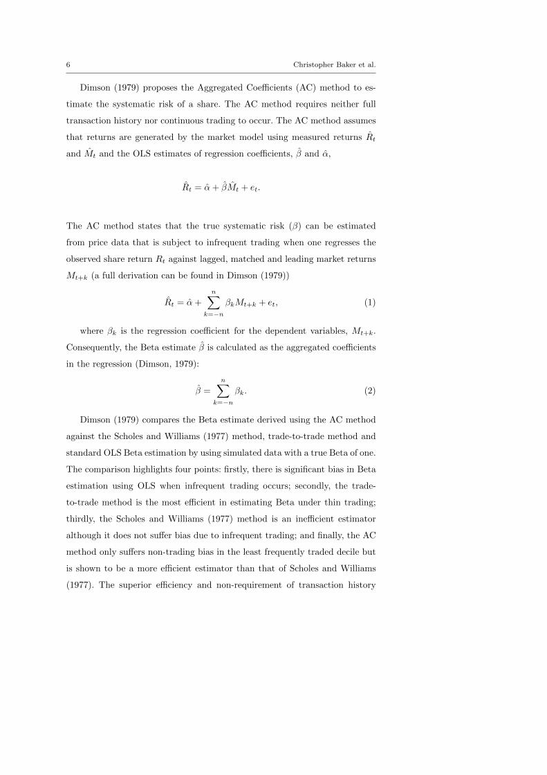
Dimson (1979) proposes the Aggregated Coefficients (AC) method to es-

timate the systematic risk of a share. The AC method requires neither full

transaction history nor continuous trading to occur. The AC method assumes

that returns are generated by the market model using measured returns Rt

and Mt and the OLS estimates of regression coefficients, β and α,

Rt = α+ βMt + et.

The AC method states that the true systematic risk (β) can be estimated

from price data that is subject to infrequent trading when one regresses the

observed share return Rt against lagged, matched and leading market returns

Mt+k (a full derivation can be found in Dimson (1979))

Rt = α+

n∑k=−n

βkMt+k + et, (1)

where βk is the regression coefficient for the dependent variables, Mt+k.

Consequently, the Beta estimate β is calculated as the aggregated coefficients

in the regression (Dimson, 1979):

β =

n∑k=−n

βk. (2)

Dimson (1979) compares the Beta estimate derived using the AC method

against the Scholes and Williams (1977) method, trade-to-trade method and

standard OLS Beta estimation by using simulated data with a true Beta of one.

The comparison highlights four points: firstly, there is significant bias in Beta

estimation using OLS when infrequent trading occurs; secondly, the trade-

to-trade method is the most efficient in estimating Beta under thin trading;

thirdly, the Scholes and Williams (1977) method is an inefficient estimator

although it does not suffer bias due to infrequent trading; and finally, the AC

method only suffers non-trading bias in the least frequently traded decile but

is shown to be a more efficient estimator than that of Scholes and Williams

(1977). The superior efficiency and non-requirement of transaction history


confirms the choice of using the Dimson (1979) method over the Scholes and

Williams (1977) method to adjust for thin trading in this paper, recalling the

necessity of adjusting for thin trading on the JSE (Bradfield, 2003).

The second adjustment to Beta estimates investigated under reference-day

risk in Acker and Duck (2007) is the method proposed by Blume (1971) when

investigating the stationarity of Beta estimates. Blume (1971) creates port-

folios of shares according to the magnitude of estimated systematic risk and

estimates the systematic risk for the portfolios for consecutive, non-overlapping

periods. The results show a tendency for the portfolios with the highest Beta

estimates (≥ 1) to decline monotonically towards 1. The portfolios with the

lowest Beta estimates tend towards 1 over time.1

Blume (1971) regresses period 2 Betas (β2) for individual securities on

those obtained from period 1 (β1) according to the following regression (where

a and b are regression coefficients and et is a zero mean error term):

β2 = a+ bβ1 + et.

The mean squared errors of the actual correlation of share returns to market

returns against the estimated value of the risk (the Beta estimate) for both

the adjusted and unadjusted Beta estimates are calculated. The mean squared

error of the adjusted estimates is consistently smaller than that of the unadjus-

ted Beta estimates, concluding that the Beta estimates adjusted according to

previous estimates result in higher accuracy even though the rate of regression

is not necessarily constant (Blume, 1971).

The final adjustment investigated in Acker and Duck (2007) is that put

forward by Vasicek (1973), who presents a method for generating Bayesian

estimates for Beta used in the market model. The prior distribution used

is normal with mean b′ and variance s′2b . The parameters b′ and s′2b are the

sample mean and variance (respectively) of the OLS Beta estimates calculated

for shares in the index.

1 All Betas were positive in Blume (1971).


Vasicek (1973) indicates that the properties of the OLS Beta estimate do

not represent satisfactory conditions for Beta estimation, even after acknow-

ledging that the OLS Beta estimate is the unbiased estimator that obtains the

lowest quadratic error.

The particular property that Vasicek (1973) challenges is:

E[β|β] = β.

The above property describes the mean of the estimator, assuming that the

true value of Beta is known. However, one would not need an estimator if the

β is known. The reverse of the above condition is true: one wants to make

an inference on β given an estimate β. Vasicek (1973) voices the need for an

estimate such that the true value of β has an equal probability of lying above

and below the Beta estimate β.

Using the normal prior distribution with mean b′ and variance s′2b , Vasicek

(1973) shows that the posterior distribution of Beta is normally distributed

with mean b′′ and variance s′′ 2b , where β is the OLS estimate of the systematic

risk and:

b′′ =(b′/s′2b + β/s2

b)

(1/s′2b + 1/s2b),

s′′ 2b =

1

(1/s′2b + 1/s2b),

s2b =

s2∑(Mt − M)2

,

s2 =

∑(Rt − α− βMt)

2

(T − 2),

where t is the time step, with t = 1, 2, ..., T .

The mean of the posterior distribution b′′ is used as the Bayesian estimate

for systematic risk. Bayesian estimators are preferred to OLS estimates for

two reasons: firstly, Bayesian estimates minimise the loss of accuracy due to

mis-estimation whereas OLS estimates minimise the loss of accuracy due to

sampling error; and secondly, Bayesian estimators incorporate previous inform-

ation and sampling knowledge into the estimate of systematic risk (Vasicek,

1973).

The literature investigating reference-day risk for Beta on the S&P500 has

verified its existence even after the relevant adjustments. Our focus is on the


JSE Top 40. This raises the questions: “Is there Beta-related reference-day

risk implicit in the JSE Top 40?”; “What is the effect of adjusting Betas on

reference-day risk in the JSE Top 40?”; and “Can we create a reference-day

independent estimate of systematic risk?”. In the remainder of the paper, we

estimate Betas independent of reference-day.

3 Data and Basic Assumptions

This paper uses the daily closing level of the All Share Index (ALSI) and

closing prices of shares making up the JSE Top 40 index over the period

January 2000 to July 2015. The data is extracted from DataStream, where

the share prices with code “P” and ALSI level with code “PI” are taken.

The companies making up the JSE Top 40 index over the period are listed in

Appendix A. Section 4 is based on the market model, Rt = α+βMt+et, which

states that a share’s returns can be modelled using market returns, where β is

the systematic risk of the company. The systematic risk can be estimated by

β, where β = cov(R;M)var(M) . We refer to the estimate of systematic risk as Beta.

In Section 4.3.1 we assume that when one calculates Beta, we are sampling

a random variable from a distribution that approximates the true systematic

risk of a company. Following Dimson (1979), we assume that share prices are

log normally distributed when simulating monthly returns.

4 Method, Results and Analysis

In this section we establish the existence of reference-day risk and demonstrate

its persistence after adjusting Betas using common adjustments.

4.1 Investigating the Existence of Reference-Day Risk

The monthly share prices (and index level) data is organised according to

trading days, the first trading day of a month does not necessarily fall on the


first calendar day of the month. Log returns for the shares and the index are

calculated for the period January 2010 to December 2014 for each of the 20

trading days (used because every month has at least 20 trading days).

Betas are calculated for each share across all trading days. We test the

different Betas for a particular share for statistically significant difference by

creating a model that includes the returns on the share and market for all

trading days. The model is restricted to test the hypothesis, H1, that all of

the Betas for a company are equal. Following that, the model is restricted

to test the hypothesis, H2, that the largest and smallest Betas for the same

company, but calculated using different trading days, are equal:

Test 1

H0 : βi = βj ∀i, j

HA : βi 6= βj for some i, j

Test 2

H0 : maxβ = min[β]

HA : maxβ 6= min[β]

The Betas that are compared in the above hypothesis test are outputs of

different regressions, with each regression using different set of data. In order

to test the hypothesis that the Betas are equal, we approximated an F -statistic

using the Pillai-Bartlett trace (see Fox et al (2013) for more).2

Upon first inspection of the unadjusted Betas, it is clear that there is an

effect on Beta when the reference-day is varied. Using the ranges of Beta, the

effect of change in reference-day is most pronounced in AngloGold Ashanti,

Anglo American Platinum and Brait SE (see Table 1). Similarly, there are also

companies for which Beta appears to be relatively constant. Using the ranges

of Beta, there appears to be little effect in Mondi PLC, Remgro and Standard

Bank across trading days. Beta remains at a relatively constant level for these

three companies across trading days. A summarized table for all companies on

the JSE Top 40 can be found in Appendix B.

2 We use the linearhypothesis function on R to determine the probability of null-

hypothesis in Test 1 and Test 2.


Smallest Ranges Largest Ranges

MNL REM STA AAP BRA AAG

Max 1.225 0.967 0.872 1.590 0.950 1.656

Min 1.016 0.721 0.621 0.897 0.089 0.499

Range 0.210 0.245 0.251 0.693 0.861 1.157

Mean 1.121 0.872 0.767 1.273 0.579 0.794

Variance 0.004 0.004 0.005 0.036 0.072 0.079

Median 1.104 0.876 0.786 1.266 0.647 0.723

Pr(H1 True) 1.000 1.000 1.000 0.987 0.992 0.968

Pr(H2 True) 0.313 0.495 0.379 0.081 0.041 0.045

Table 1: Smallest and Largest ranges in unadjusted Beta

The differences in Beta could have adverse repercussions for share portfolio

construction. For example, consider a risk-averse investor who wishes to build

a share portfolio that is weakly correlated with the market (positive Beta less

than one). If the investor happens to calculate Beta for AngloGold Ashanti and

Brait on a day that yields the lowest Betas, the investor could achieve an overall

Beta for his portfolio ranging between 0.089 - if the portfolio is made entirely

of Brait SA - and 0.499 - if the portfolio is made entirely of AngloGold Ashanti

- according to proportions of the shares held. One expects this portfolio to earn

returns that are correlated with the market, but not as extreme. The portfolio

value will increase (less so than the market) if the market performs well, but

is also partially shielded from declines in the performance of the market.

However, the investor has unknowingly created a portfolio with a worst-

case scenario Beta ranging between 1.656 and 0.950, the largest unadjusted

Betas for AngloGold and Brait, respectively. The systematic risk of the in-

vestor’s portfolio has been misestimated. The investor is holding a portfolio

where the returns are more pronounced than the market. Market changes will

exaggerate the fluctuations in value of the portfolio. Furthermore, the investor

could be slow to react to a sharp decline in the market because he/she believes

his/her portfolio is weakly correlated with the market.


The tests of statistical significance reveal that we cannot reject H1 for any

of the companies. However, different results are reached when testing H2. We

can reject H2 at the 10% significance level for 16 out of the 40 of the companies.

Furthermore, we can reject H2 at the 5% significance level for six out of the

40 companies.

The results show that there are companies with significant differences in

Beta when the reference-day is changed.

Variation in Beta over reference-days means that investors valuing com-

panies based on future cash flows (dividends) discounted at a risk-adjusted

rate, based on the CAPM model, risk inaccurately valuing shares. The in-

vestor will overstate the theoretical share price if the Beta is calculated using

reference-days that produce a low Beta, resulting in a lower than appropriate

discount rate being used, thus valuing the share above the market price. The

investor would think this share is priced at a discount, when the market value

of the share could reflect its true value.

The fact that 16 of the 40 of the companies considered proved to have

at least one pair of Betas that are significantly different at the 10% level is

a concern. There is potential for a large proportion of the total number of

shares listed on the JSE to be adversely affected by reference-day risk when

estimating systematic risk.

The estimates of systematic risk that most institutional investors use are

not the traditional Beta estimates. Therefore, it is important to investigate

whether the reference-day variation in systematic risk persists after adjusting

the traditional Beta by methods commonly used in practice.

4.2 Establishing that Reference-Day Risk Persists after Common

Adjustments

In this section we establish that Reference-Day Risk persists after Beta is

adjusted by the Blume (1971), Dimson (1979) and Vasicek (1973) methods.

When testing for the unadjusted Betas, we tested whether the Betas were


statistically different for each company. The method employed allowed us to

test the difference between these regression coefficients, that were a result

of different regressions. However, this method cannot be employed for the

adjusted Betas as these were not regression coefficients, but rather regression

coefficients that had been adjusted. It is for this reason that we use the range

of Beta estimates as a measure of reference-day risk.

4.2.1 Blume (1971)-adjusted Beta

Beta is calculated for each company, as per Section 4.1, over the periods Janu-

ary 2000 to December 2004 (Period 1) and January 2005 to December 2009

(Period 2), across 20 trading days.

For each trading day we create a linear model with the Period 1 Betas

as the explanatory variable and Period 2 Betas as the dependent variable.

Blume (1971)-adjusted Betas for the period January 2010 to December 2014

are the values that result from inserting the Period 2 Betas into the model as

explanatory variables.

We are unable to calculate the Blume (1971)-adjusted Betas for some of the

companies (British American Tobacco, Capitec Bank, Investec PLC, Kumba

Iron Ore, Mondi Ltd, Mondi PLC, Reinet Investments, Remgro and Vodacom

Group) because of insufficient price history.

The largest range out of the companies investigated is 0.783 (Old Mutual),

where the largest Blume (1971)-adjusted Beta is 1.479 and the smallest is

0.696. The smallest range is 0.256 (SAB Miller), where the largest Blume

(1971)-adjusted Beta is 0.831 and the smallest is 0.575.

A summary table showing the Blume-adjusted Betas for all companies can

be found in Appendix C.

The Blume (1971)-adjusted Betas increase the reference-day ranges for 19

out of 31 companies, with the range for Old Mutual increasing by 81%. As a

result, we conclude that the Blume (1971)-adjustment does not consistently

decrease the ranges among Betas conditioned on reference day.


4.2.2 Dimson (1979)-adjusted Betas

We create a multifactor model that models the log returns of a share according

to leading, current and lagged log returns of the index. We use one leading

and three lagged index return vectors.

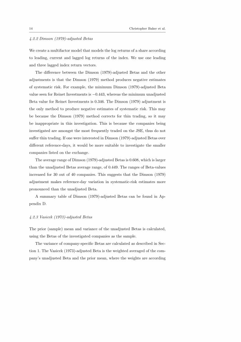
The difference between the Dimson (1979)-adjusted Betas and the other

adjustments is that the Dimson (1979) method produces negative estimates

of systematic risk. For example, the minimum Dimson (1979)-adjusted Beta

value seen for Reinet Investments is −0.443, whereas the minimum unadjusted

Beta value for Reinet Investments is 0.346. The Dimson (1979) adjustment is

the only method to produce negative estimates of systematic risk. This may

be because the Dimson (1979) method corrects for thin trading, so it may

be inappropriate in this investigation. This is because the companies being

investigated are amongst the most frequently traded on the JSE, thus do not

suffer thin trading. If one were interested in Dimson (1979)-adjusted Betas over

different reference-days, it would be more suitable to investigate the smaller

companies listed on the exchange.

The average range of Dimson (1979)-adjusted Betas is 0.608, which is larger

than the unadjusted Betas average range, of 0.449. The ranges of Beta-values

increased for 30 out of 40 companies. This suggests that the Dimson (1979)

adjustment makes reference-day variation in systematic-risk estimates more

pronounced than the unadjusted Beta.

A summary table of Dimson (1979)-adjusted Betas can be found in Ap-

pendix D.

4.2.3 Vasicek (1973)-adjusted Betas

The prior (sample) mean and variance of the unadjusted Betas is calculated,

using the Betas of the investigated companies as the sample.

The variance of company-specific Betas are calculated as described in Sec-

tion 1. The Vasicek (1973)-adjusted Beta is the weighted averaged of the com-

pany’s unadjusted Beta and the prior mean, where the weights are according


to the variance of the company Beta and the sample variance, respectively.

The estimate is described in Section 1.

The Vasicek (1973) method adjusts the unadjusted Beta towards the mar-

ket average. The resulting Vasicek (1973)-adjusted Betas are similar to those

of the unadjusted Betas, as one would expect. The Vasicek (1973) adjustment

has reduced the occurrence of extreme differences. The Beta ranges for 35 of

the JSE Top 40 companies exhibited lower reference-day ranges than unadjus-

ted Betas. A summary table of Vasicek (1973)-adjusted Betas can be found in

Appendix E.

4.2.4 Comments on Common Adjustments to Beta

It is difficult to prove statistically significant difference (as we did in Section

4.1) in the adjustments that we investigate. This difficulty is because of the

construction of the estimates using the respective adjustments. As a result,

we use the relative average range of estimates an indication of the level of

reference-day risk.

From what we have observed, it is clear that reference-day risk in estimating

the systematic-risk of some companies persist even after common adjustments.

A method for estimating systematic risk that is independent of reference-day

risk is needed.

4.3 Simulating a Reference-Day Independent Point-Estimate of Systematic

Risk

Our primary goal in this paper is to provide a method to estimate a point-

estimate (or single value) of Beta that is independent of reference-day. Given

twenty estimates of Beta for each company, we may then take the average in

order to determine a Beta independent of reference-day. However, this may in-

troduce errors due to small sample size (see Ader et al (2008:373) for more). In

this section, we investigate the feasibility of using a bootstrapped Beta distri-

bution to estimate systematic risk, in which we bootstrap a Beta distribution


for the companies under investigation. If we were able to recover the underly-

ing Beta distribution, we would use the expected value of the distribution as

a point-estimate of the true systematic risk and hence, our primary focus is

on the point-estimate of Beta that is independent of reference-day risk. Our

focus is not to estimate the distribution of Beta.

We estimate Betas independent of reference-day as follows. Suppose, each

share has an underlying Beta value that is not directly observable in the mar-

ket. Under this assumption of an underlying Beta value, we simulate returns

data for both the company and the market-index using the correlation relation-

ship through the Beta-distribution. We simulate 60 sequences of 60 returns-

pair for the company and the market index. Each sequence of 60 returns-pair

are a sequence of returns for 60 months assuming an arbitrary reference day.

A Beta estimate may then be calculated for each 60 returns sequence. We,

then, chose 20 such sequences such that the variance of Beta for the chosen

sequences were maximised. Then, using the simulated returns, we may use a

non-parametric bootstrap-approach to estimate an implied Beta estimate, and

compare this Beta estimate to the expected value of the originally assumed un-

derlying Beta distribution. Since price is returns in the market, this approach

allows us to estimate the underlying Beta.

4.3.1 Evaluating the Feasibility of Bootstrapping a Beta Distribution

Index levels and share prices are created under the assumption that index

levels and share prices are log normally distributed. Both sequences are based

on the same underlying Brownian motion (Bt ∼ N(0, t)) so that the level of

correlation of log returns between the two sequences (systematic risk) can be

controlled.

Suppose the value of the index at time t (in years) is e0.01t+0.1Bt and

the share price at the same time is e0.01t+0.1Y Bt . We assume that the Beta

we calculate on a certain reference-day comes from a distribution that arises

because of reference-day variation and approximates the true systematic risk.


Let Y be the distribution assigned to the underlying distribution of Beta. The

initial distribution for Y is chosen as N(1.5, 0.52).

We simulate 60 strings of monthly log returns (of length 60 as in Section

4.1 and Section 4.2) for the company and the index. Each string represents a

trading day. We randomly select a share price for each monthly return, out

of the possible trading days, and use the random sequence of stock returns

and the corresponding index returns to calculate an estimate of systematic

risk. The process of randomly selecting elements and calculating Beta is re-

peated 100 000 times per share so that a bootstrapped Beta distribution can

be graphed.

The resulting frequency distribution is compared to that of Y, following

which the effect of changing the parameter values of Y is assessed. We proceed

to evaluate the effect of changing the distribution of Y to a uniform distribu-

tion and investigate the effects of changing the parameter values of Y on the

bootstrapped Beta distribution.

When Y is normal, the simulated mean value is consistently within half a

standard deviation of the mean of Y. For example, when Y is normal with a

mean of 1.5 and standard deviation of 0.5, the resulting bootstrapped Beta

distribution has a mean value of 1.450. This is shown in Figure 1a, with a

N(1.450, 0.1042) distribution fitted in red and the distribution of Y fitted in

green.

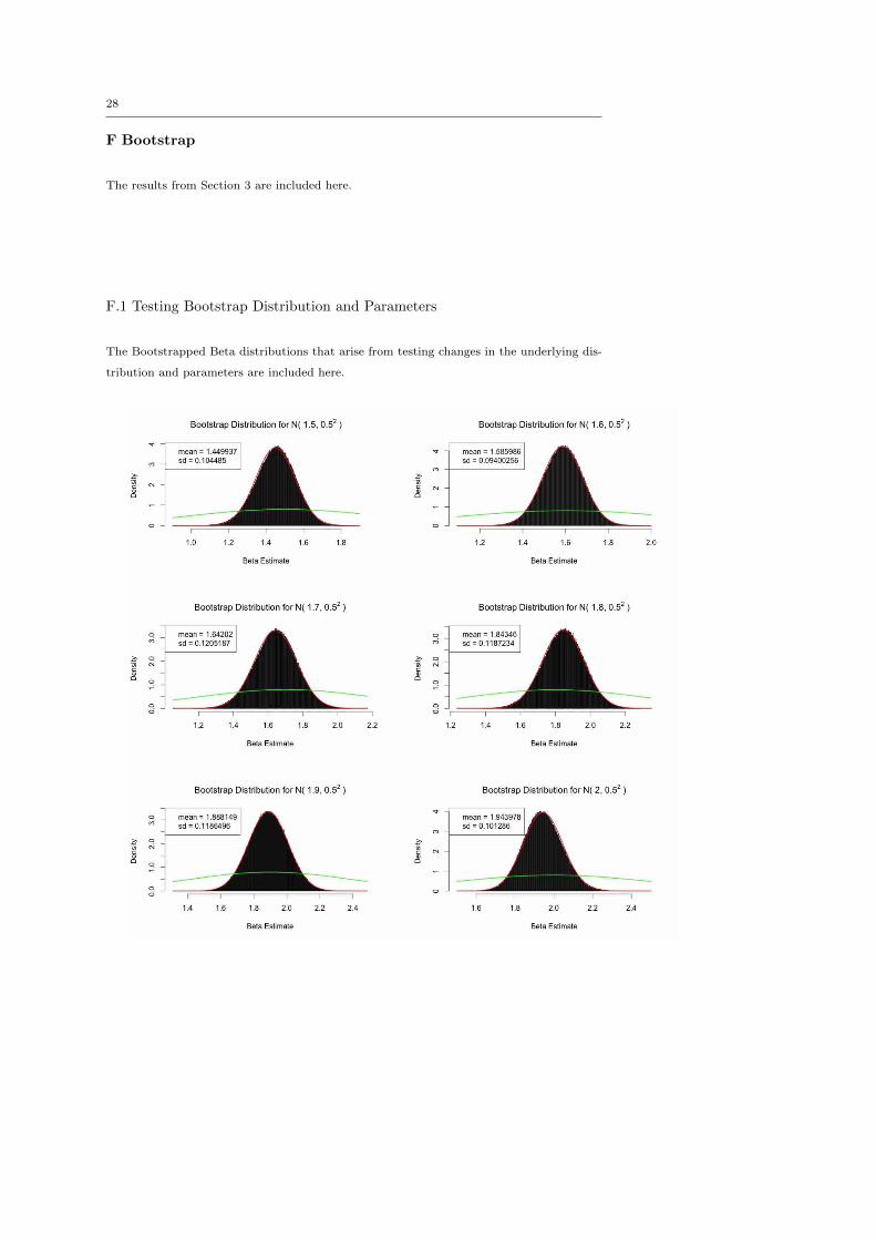
As the mean parameter of Y is increased, the resulting bootstrapped Beta

distributions remain centred within 0.05 of the mean of Y. Moreover, the

standard deviation of the bootstrapped Beta distributions fluctuate slightly

around 0.1 in comparison to the standard deviation of Y, which is 0.5. This is

shown graphically in Appendix F.1.

When the standard deviation parameter of Y is increased, the resulting

bootstrapped Beta distribution displays an increasing standard deviation as

well. Despite the increasing standard deviation, the mean parameter of the

bootstrapped Beta distribution remains within half of a standard deviation

(standard deviation of the bootstrapped Beta distribution) of the mean of Y.


Appendix F.1 shows the bootstrapped Beta distributions that arise when the

standard deviation of the Y is increased steadily.

When Y is changed to a uniform distribution, the resulting bootstrapped

Beta distribution remains normal and becomes more concentrated around the

mean of Y. The standard deviation of the bootstrapped Beta distributions in-

creases steadily as the difference between the parameters of the Y is increased.

Figure 1b displays the resulting bootstrapped Beta distribution when Y

is uniform with parameters 1 and 1.5. The bootstrapped Beta distribution is

clearly centred closely around 1.25, the mean value of Y. Graphs for different

parameter values of the underlying uniform Beta distribution are exhibited in

Appendix F.1.

(a) bootstrapped Beta distribution when Y is

normally distributed

(b) bootstrapped Beta distribution when Y is

uniformly distributed

Figure 1: bootstrapped Beta distributions

4.3.2 Application of the Bootstrapped Beta

A bootstrapped Beta distribution is generated, as above in Section 4.3.1, for

each of the companies under investigation.

The bootstrapped Beta distributions for the companies are normally dis-

tributed and centred approximately around the average unadjusted Beta es-

timates, where the average is calculated over the 20 trading days.


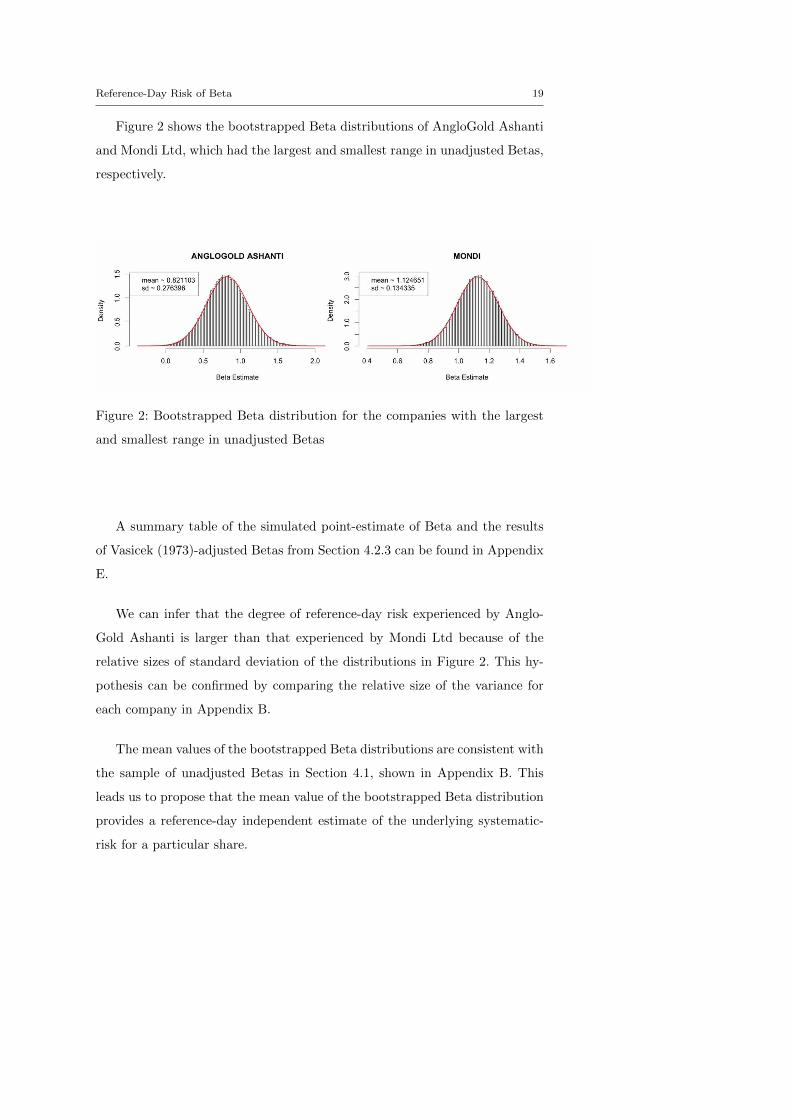
Figure 2 shows the bootstrapped Beta distributions of AngloGold Ashanti

and Mondi Ltd, which had the largest and smallest range in unadjusted Betas,

respectively.

Figure 2: Bootstrapped Beta distribution for the companies with the largest

and smallest range in unadjusted Betas

A summary table of the simulated point-estimate of Beta and the results

of Vasicek (1973)-adjusted Betas from Section 4.2.3 can be found in Appendix

E.

We can infer that the degree of reference-day risk experienced by Anglo-

Gold Ashanti is larger than that experienced by Mondi Ltd because of the

relative sizes of standard deviation of the distributions in Figure 2. This hy-

pothesis can be confirmed by comparing the relative size of the variance for

each company in Appendix B.

The mean values of the bootstrapped Beta distributions are consistent with

the sample of unadjusted Betas in Section 4.1, shown in Appendix B. This

leads us to propose that the mean value of the bootstrapped Beta distribution

provides a reference-day independent estimate of the underlying systematic-

risk for a particular share.


5 Conclusions

This paper set out to establish whether there is reference-day risk when estim-

ating systematic risk in the JSE Top 40. We can conclude that reference-day

risk exists and creates additional uncertainty for investors who intend to cre-

ate share portfolios, value companies or manage their capital. This raises the

need for an estimate of systematic risk that is reference-day independent.

Having proved the existence of reference-day risk when estimating system-

atic risk in the JSE Top 40, this paper investigates whether the reference-day

variation in estimates persists after being adjusted by the Blume (1971), Dim-

son (1979) and Vasicek (1973) methods. It is shown that the Blume (1971) and

Dimson (1979) adjustments do not reduce reference-day variation in estimat-

ing systematic risk. In fact, in some cases the variation is more pronounced,

thus further implying the necessity for a reference-day independent estimate

of systematic risk.

The final part of this paper set out to simulate a reference-day independent

estimate of systematic risk. We first establish that we are able to recover

the mean value of a set underlying Beta distribution, but not the standard

deviation, by bootstrapping a distribution for Beta using the available monthly

returns over all trading days. For the shares on the JSE Top 40, the expected

value of a reference-day independent Beta using the bootstrapped method was

approximately equal to the average of the twenty Betas estimated for each

reference day. Despite this, we assert that the bootstrap method in this paper

provides some benefits. Firstly, given the sample size of twenty reference-day

dependent Betas, any distortion in the sample may distort the average (i.e., the

estimate of the reference-day independent Beta estimated using the average

of twenty Betas). Secondly, this work provides a basis for further analysis into

estimating the standard deviation of a reference-day independent Beta.

Acknowledgements This work is based on the research supported in part by the National

Research Foundation (NRF) of South Africa for the Grant No. 93649. Any opinion, finding

and conclusion or recommendation expressed in this material is that of the authors and


the NRF does not accept any liability in this regard. Additional funding was provided by

University of Cape Town Research Office through the Research Development Grant and the

Conference Travel Grant.

References

Acker D, Duck NW (2007) Reference-day risk and the use of monthly re-

turns data. Journal of Accounting, Auditing and Finance 22(4):527 – 557,

URL http://search.ebscohost.com/login.aspx?direct=true&db=buh&

AN=27157515&site=ehost-live

Ader HJ, Ader M, et al (2008) Advising on research methods: A consultant’s

companion. Johannes van Kessel Publishing.

Blume ME (1971) On the assessment of risk. Journal of Finance 26(1):1 – 10,



BNP Paribas Cadiz Securities (2014) Estimating betas for JSE-listed compan-

ies and indices

Bowie D, Bradfield D (1993) Improved beta estimation on the JSE: a simula-

tion study. South African Journal of Business Management 24:118–123

Bradfield D (2003) Investment basics xlvi. on estimating the beta coefficient.

Investment Analysts Journal 57:47–53

Cademartori D, Romo C, Campos R, Galea M (2003) Robust estimation of

systematic risk using the t distribution in the chilean stock markets. Ap-

plied Economics Letters 10(7):447, URL http://search.ebscohost.com/

login.aspx?direct=true&db=buh&AN=10088858&site=ehost-live

Cohen KJ, Hawawini GA, Maier SF, Schwartz RA, Whitcomb DK (1983) Fric-

tion in the trading process and the estimation of systematic risk. Journal

of Financial Economics 12(2):263 – 278, doi: http://dx.doi.org/10.1016/

0304-405X(83)90038-7, URL http://www.sciencedirect.com/science/

article/pii/0304405X83900387

Dimitrov V, Govindaraj S (2007) Reference-day risk: Observations and ex-

tensions. Journal of Accounting, Auditing and Finance 22(4):559 – 572,




Dimson E (1979) Risk measurement when shares are subject to infrequent

trading. Journal of Financial Economics 7(2):197 – 226, doi: http://dx.doi.

org/10.1016/0304-405X(79)90013-8, URL http://www.sciencedirect.

com/science/article/pii/0304405X79900138

Fox J, Friendly M, Weisberg S (2013) Hypothesis tests for multivariate linear

models using the car package. R J 5(1):39–52

Gonzalez M, Rodriguez A, Stein R (2014) Adjusted betas under

reference-day risk. Engineering Economist 59(1):79 – 88, URL

http://search.ebscohost.com/login.aspx?direct=true&db=aph&


Marsh P (1979) Equity rights issues and the efficiency of the uk stock market.

Journal of Finance 34(4):839 – 862, URL http://search.ebscohost.com/

login.aspx?direct=true&db=buh&AN=4656321&site=ehost-live

Scholes M, Williams J (1977) Estimating betas from nonsynchronous data.

Journal of Financial Economics 5(3):309 – 327, doi: http://dx.doi.org/

10.1016/0304-405X(77)90041-1, URL http://www.sciencedirect.com/

science/article/pii/0304405X77900411

Sharpe WF (1963) A simplified model for portfolio analysis. Management Sci-

ence 9(2):277 – 293, URL http://search.ebscohost.com/login.aspx?

direct=true&db=buh&AN=7451896&site=ehost-live

Vasicek OA (1973) A note on using cross-sectional information in bayesian

estimation of security bias. Journal of Finance 28(5):1233 – 1239,



23

Appendices

A Company List

The company names are shortened in order to fit the tables. The full company names and

corresponding codes are included here.

Company Code Company Code

Anglo American Platinum Ltd AAP Mondi Ltd MNL

Anglo American PLC AA Mondi PLC MNP

AngloGold Ashanti Ltd AGA Mr Price Group Ltd MRP

Aspen Pharmaceuticals Holding ASP MTN Group Ltd MTN

Barclays Africa Group Ltd BAR Naspers Ltd NAS

BHP Billiton PLC BHP Nedbank Group Ltd NED

Bidvest Group Ltd BID Netcare Ltd NET

Brait S.E BRA Old Mutual PLC OLD

British American Tobacco PLC BRI Rand Merchant Insurance Holdings RAN

Capital and Counties Prop PLC CC Reinet Investments SCA. REI

Capitec Bank CAP Remgro Ltd REM

Compagnie Financire Richemont SA RIC RMB Holdings Ltd RMB

Discovery Ltd DIS SABMiller PLC SAB

FirstRand Ltd FIR Sanlam Ltd SAN

Growthpoint Properties Ltd GRO Sasol SAS

Intu Properties PLC INT Shoprite Holdings Ltd SHO

Investec Ltd INL Standard Bank Group Ltd STA

Investec PLC INP Steinhoff International Holdings Ltd STE

Kumba Iron Ore KUM Tiger Brands Ltd TIG

Mediclinic International Ltd MED Vodacom Group Ltd VOD

MMI Holdings Ltd MMI Woolworths Holdings Ltd WOO

24B

Unadjusted

Beta

Tab

le2:

Un

ad

just

edB

eta

Valu

esfo

rea

chtr

ad

ing

day

(firs

t20

share

s)

Tradin

gD

ay

AAP

AA

AG

AASP

BHP

BAR

BID

BRA

BRI

CAP

RIC

DIS

FIR

GRO

INT

INL

INP

KUM

MM

IM

TN

Max

1,5

91,7

34

1,6

56

0,9

56

1,8

16

1,0

21

1,0

44

0,9

50,5

60,5

54

1,5

05

0,8

53

1,0

07

0,5

34

1,2

11

1,3

95

1,4

26

1,4

12

1,0

86

0,9

12

Min

0,8

97

1,4

56

0,4

99

0,5

33

1,4

63

0,6

52

0,6

80,0

89

0,0

95

0,0

47

1,0

08

0,4

87

0,5

62

0,1

95

0,7

28

1,0

15

1,0

71

0,9

33

0,6

49

0,3

03

Range

0,6

93

0,2

78

1,1

57

0,4

23

0,3

53

0,3

69

0,3

64

0,8

61

0,4

65

0,5

06

0,4

97

0,3

66

0,4

45

0,3

39

0,4

83

0,3

80,3

56

0,4

79

0,4

37

0,6

09

Mean

1,2

73

1,5

88

0,7

94

0,7

53

1,6

57

0,8

36

0,8

68

0,5

79

0,3

90,2

98

1,2

77

0,7

36

0,8

33

0,4

20,8

83

1,2

77

1,2

78

1,2

09

0,8

52

0,6

38

Varia

nce

0,0

36

0,0

06

0,0

79

0,0

17

0,0

12

0,0

09

0,0

14

0,0

72

0,0

16

0,0

24

0,0

30,0

09

0,0

11

0,0

09

0,0

28

0,0

07

0,0

06

0,0

24

0,0

15

0,0

26

Media

n1,2

66

1,5

87

0,7

23

0,7

28

1,6

59

0,8

24

0,9

02

0,6

47

0,3

95

0,3

03

1,2

29

0,7

51

0,8

48

0,4

39

0,7

86

1,2

86

1,2

78

1,2

35

0,8

36

0,6

06

Pr(H1

True)

0,9

87

10,9

68

10,9

05

0,9

83

0,8

83

0,9

92

0,7

95

0,9

92

0,7

95

0,9

99

0,9

78

0,9

99

0,3

73

10,9

99

0,9

98

0,9

67

0,7

74

Pr(H2

True)

0,0

81

0,3

13

0,0

45

0,3

97

0,0

82

0,1

28

0,0

80,0

41

0,0

50,1

53

0,0

85

0,1

54

0,0

81

0,1

51

0,1

17

0,1

06

0,1

42

0,1

70,2

43

0,0

24

Tab

le3:

Un

ad

just

edB

eta

Valu

esfo

rea

chtr

ad

ing

day

(sec

on

d20

share

s)

Tradin

gD

ay

MED

MNL

MNP

MRP

NAS

NED

NET

OLD

RM

BREI

REM

SAB

SAN

SAS

SHO

STA

STE

TIG

VO

DW

OO

Max

0,7

36

1,2

25

1,3

36

0,9

36

1,5

81

0,8

26

0,7

96

1,2

55

1,0

33

0,6

98

0,9

67

0,8

77

1,0

57

1,3

38

0,6

91

0,8

72

1,0

61

0,9

60,8

17

1,0

99

Min

0,2

87

1,0

16

1,0

64

0,5

67

0,9

70,3

74

0,4

98

0,8

23

0,5

32

0,3

46

0,7

21

0,4

99

0,7

31

0,8

83

0,2

27

0,6

21

0,6

63

0,4

66

0,3

63

0,4

17

Range

0,4

49

0,2

10,2

73

0,3

70,6

11

0,4

53

0,2

98

0,4

32

0,5

01

0,3

52

0,2

45

0,3

78

0,3

26

0,4

55

0,4

63

0,2

51

0,3

98

0,4

93

0,4

53

0,6

82

Mean

0,5

73

1,1

21

1,1

75

0,7

32

1,1

99

0,6

36

0,6

45

1,0

77

0,8

39

0,5

39

0,8

72

0,7

55

0,9

04

1,1

46

0,4

71

0,7

67

0,8

60,7

25

0,5

42

0,7

59

Varia

nce

0,0

13

0,0

04

0,0

04

0,0

11

0,0

35

0,0

26

0,0

06

0,0

19

0,0

18

0,0

09

0,0

04

0,0

09

0,0

07

0,0

19

0,0

22

0,0

05

0,0

15

0,0

23

0,0

15

0,0

56

Media

n0,5

69

1,1

04

1,1

65

0,6

98

1,1

78

0,6

64

0,6

55

1,0

86

0,8

31

0,5

37

0,8

76

0,7

78

0,8

85

1,1

28

0,4

59

0,7

86

0,8

33

0,7

28

0,4

99

0,7

58

Pr(H1

True)

0,9

78

11

10,9

0,4

36

10,9

65

0,7

94

0,9

79

10,9

50,9

95

0,9

53

0,9

92

0,9

98

0,9

95

0,8

91

0,9

94

0,5

81

Pr(H2

True)

0,0

51

0,4

95

0,3

79

0,2

96

0,0

37

0,0

32

0,2

22

0,1

12

0,0

43

0,0

91

0,2

40,0

55

0,1

51

0,0

95

0,2

0,3

09

0,1

53

0,0

63

0,1

12

0,0

47

25C

BlumeAdjustment T

able

4:

Blu

me-

ad

just

edB

eta

Valu

esfo

rea

chtr

ad

ing

day

(sec

on

d20

share

s)

Tradin

gD

ay

AAP

AA

AG

AASP

BHP

BAR

BID

BRA

BRI

CAP

RIC

DIS

FIR

GRO

INT

INL

INP

KUM

MM

IM

TN

Max

1,8

38

1,6

11

0,8

50

0,7

87

1,4

43

0,9

20

1,0

10

0,9

72

1,0

19

0,8

34

0,9

48

0,6

99

0,9

41

1,2

61

0,9

45

1,1

51

Min

1,1

30

1,2

01

0,5

42

0,2

07

1,0

88

0,4

82

0,6

08

0,3

65

0,5

22

0,4

63

0,5

97

0,2

13

0,4

07

0,6

67

0,3

36

0,5

91

Range

0,7

08

0,4

09

0,3

08

0,5

80

0,3

55

0,4

38

0,4

02

0,6

08

0,4

98

0,3

72

0,3

51

0,4

86

0,5

34

0,5

95

0,6

09

0,5

60

Mean

1,5

08

1,4

63

0,7

15

0,4

87

1,2

68

0,6

83

0,7

76

0,7

07

0,8

04

0,6

48

0,7

72

0,4

93

0,6

63

0,9

88

0,6

39

0,8

50

Varia

nce

0,0

27

0,0

16

0,0

09

0,0

26

0,0

10

0,0

13

0,0

10

0,0

29

0,0

28

0,0

08

0,0

14

0,0

17

0,0

30

0,0

31

0,0

26

0,0

31

Media

n1,4

93

1,4

97

0,7

26

0,4

92

1,2

47

0,6

86

0,7

54

0,7

48

0,8

48

0,6

61

0,7

80

0,4

72

0,6

41

1,0

26

0,6

45

0,8

05

Tab

le5:

Blu

me-

ad

just

edB

etas

for

each

trad

ing

day

(sec

on

d20

share

s)

Tradin

gD

ay

MED

MNL

MNP

MRP

NAS

NED

NET

OLD

RM

BREI

REM

SAB

SAN

SAS

SHO

STA

STE

TIG

VO

DW

OO

Max

0,6

51

0,8

57

1,0

69

1,0

27

0,9

49

1,4

79

0,9

23

0,8

31

0,9

26

1,2

50

0,8

62

0,9

73

1,2

42

0,7

84

1,0

58

Min

0,2

96

0,2

20

0,7

56

0,5

05

0,5

61

0,6

96

0,5

58

0,5

75

0,4

48

0,9

66

0,3

99

0,5

67

0,6

06

0,4

40

0,4

78

Range

0,3

55

0,6

36

0,3

13

0,5

22

0,3

88

0,7

83

0,3

65

0,2

56

0,4

78

0,2

84

0,4

63

0,4

06

0,6

35

0,3

44

0,5

81

Mean

0,4

83

0,5

93

0,8

76

0,7

58

0,7

25

1,0

96

0,7

35

0,7

30

0,7

09

1,1

08

0,6

00

0,7

56

0,9

11

0,6

28

0,7

25

Varia

nce

0,0

11

0,0

29

0,0

07

0,0

19

0,0

12

0,0

40

0,0

14

0,0

05

0,0

11

0,0

04

0,0

16

0,0

13

0,0

46

0,0

10

0,0

27

Media

n0,4

70

0,6

52

0,8

61

0,7

70

0,7

01

1,0

72

0,7

42

0,7

35

0,7

32

1,1

06

0,5

83

0,7

42

0,9

33

0,6

49

0,7

39

26D

Dim

son

Adjustment

Tab

le6:

Dim

son

-ad

just

edB

etas

for

each

trad

ing

day

(firs

t20

share

s)

Tradin

gD

ay

AAP

AA

AG

AASP

BHP

BAR

BID

BRA

BRI

CAP

RIC

DIS

FIR

GRO

INT

INL

INP

KUM

MM

IM

TN

Max

2,7

32

2,8

63

1,2

60

0,0

36

2,7

64

1,0

42

0,8

19

0,8

15

0,0

15

0,0

98

1,4

35

0,4

06

1,2

32

0,1

60

1,1

60

1,2

72

1,2

04

1,7

40

0,6

24

0,9

57

Min

1,6

69

2,1

11

0,1

76

-0,5

90

2,2

19

0,4

82

0,4

99

0,1

30

-0,7

55

-0,9

08

0,9

29

-0,0

98

0,6

89

-0,4

37

0,7

26

0,9

80

0,9

50

0,9

05

-0,0

18

0,2

10

Range

1,0

64

0,7

52

1,0

84

0,6

26

0,5

45

0,5

59

0,3

21

0,6

85

0,7

70

1,0

06

0,5

05

0,5

05

0,5

42

0,5

97

0,4

34

0,2

92

0,2

54

0,8

35

0,6

42

0,7

47

Mean

2,3

35

2,4

17

0,6

69

-0,2

54

2,3

87

0,7

75

0,6

82

0,4

19

-0,4

09

-0,4

11

1,2

01

0,1

79

0,9

76

-0,1

83

0,8

81

1,1

20

1,1

00

1,3

31

0,3

09

0,7

14

Varia

nce

0,0

92

0,0

44

0,0

74

0,0

34

0,0

22

0,0

23

0,0

09

0,0

38

0,0

51

0,0

55

0,0

19

0,0

21

0,0

20

0,0

24

0,0

10

0,0

06

0,0

04

0,0

66

0,0

34

0,0

35

Media

n2,4

15

2,3

90

0,6

70

-0,2

97

2,3

35

0,7

63

0,6

87

0,4

01

-0,4

35

-0,3

66

1,1

89

0,1

90

0,9

76

-0,1

62

0,8

95

1,1

38

1,1

12

1,3

50

0,3

02

0,7

67

Tab

le7:

Dim

son

-ad

just

edB

etas

for

each

trad

ing

day

(sec

on

d20

share

s)

Tradin

gD

ay

MED

MNL

MNP

MRP

NAS

NED

NET

OLD

RM

BREI

REM

SAB

SAN

SAS

SHO

STA

STE

TIG

VO

DW

OO

Max

0,9

97

1,3

55

1,4

86

0,3

84

1,1

86

0,7

57

0,6

49

0,9

46

1,2

30

0,1

79

0,7

44

0,6

42

1,0

21

2,0

34

-0,1

57

1,1

74

2,2

05

0,2

67

0,8

06

0,1

89

Min

0,6

49

0,3

76

0,4

25

-0,1

87

0,5

71

0,3

16

0,1

33

0,4

43

0,7

03

-0,4

43

0,3

20

0,2

16

0,6

35

1,5

76

-1,0

92

0,8

09

1,3

97

-0,2

59

0,3

69

-0,4

39

Range

0,3

48

0,9

79

1,0

62

0,5

70

0,6

15

0,4

41

0,5

16

0,5

03

0,5

27

0,6

22

0,4

24

0,4

26

0,3

86

0,4

58

0,9

35

0,3

65

0,8

08

0,5

26

0,4

37

0,6

28

Mean

0,8

42

0,8

28

0,9

39

0,0

94

0,8

61

0,5

09

0,3

83

0,7

15

1,0

26

-0,1

86

0,5

14

0,4

01

0,8

40

1,7

98

-0,4

84

0,9

68

1,8

31

0,0

25

0,5

90

-0,1

26

Varia

nce

0,0

10

0,0

80

0,0

91

0,0

20

0,0

36

0,0

19

0,0

19

0,0

16

0,0

21

0,0

42

0,0

14

0,0

12

0,0

14

0,0

13

0,0

73

0,0

10

0,0

57

0,0

25

0,0

19

0,0

29

Media

n0,8

32

0,7

92

0,8

71

0,0

69

0,8

17

0,4

71

0,3

72

0,7

05

1,0

40

-0,2

80

0,5

22

0,3

90

0,8

59

1,8

24

-0,4

21

0,9

46

1,8

12

0,0

48

0,5

91

-0,1

17

27E

VasicekAdjustment T

able

8:

Vasi

cek-a

dju

sted

Bet

aV

alu

esfo

rea

chtr

ad

ing

day

(firs

t20

share

s)

Tradin

gD

ay

AAP

AA

AG

AASP

BHP

BAR

BID

BRA

BRI

CAP

RIC

DIS

FIR

GRO

INT

INL

INP

KUM

MM

IM

TN

Max

1,4

28

1,5

45

1,4

82

0,9

48

1,6

14

1,0

07

1,0

32

0,9

41

0,5

90

0,5

79

1,3

89

0,8

57

0,9

99

0,5

87

1,1

83

1,3

19

1,3

50

1,3

12

1,0

66

0,9

06

Min

0,8

96

1,3

61

0,5

12

0,5

47

1,3

78

0,5

99

0,6

89

0,1

05

0,1

46

0,0

71

0,9

90

0,5

03

0,5

77

0,2

44

0,7

40

0,9

98

1,0

47

0,9

27

0,6

60

0,3

45

Range

0,5

32

0,1

84

0,9

70

0,4

01

0,2

36

0,4

08

0,3

42

0,8

36

0,4

44

0,5

08

0,3

98

0,3

54

0,4

22

0,3

43

0,4

43

0,3

21

0,3

03

0,3

85

0,4

06

0,5

61

Mean

1,1

92

1,4

47

0,8

01

0,7

37

1,5

05

0,8

22

0,8

59

0,5

79

0,4

42

0,3

19

1,2

26

0,7

33

0,8

15

0,4

55

0,8

93

1,2

30

1,2

38

1,1

66

0,8

59

0,6

56

Varia

nce

0,0

19

0,0

03

0,0

58

0,0

12

0,0

06

0,0

11

0,0

12

0,0

61

0,0

15

0,0

25

0,0

19

0,0

08

0,0

12

0,0

08

0,0

22

0,0

05

0,0

05

0,0

13

0,0

14

0,0

22

Media

n1,1

93

1,4

59

0,7

53

0,7

09

1,5

28

0,8

19

0,8

60

0,6

64

0,4

57

0,3

29

1,2

52

0,7

47

0,8

43

0,4

79

0,8

23

1,2

36

1,2

43

1,1

89

0,8

65

0,6

43

Poin

t-E

stim

ate

1,2

63

1,5

90

0,8

21

0,7

26

1,6

54

0,8

08

0,8

58

0,5

77

0,4

06

0,2

99

1,2

90

0,7

22

0,8

07

0,4

25

0,8

96

1,2

80

1,2

91

1,2

26

0,8

62

0,6

42

Tab

le9:

Vasi

cek-a

dju

sted

Bet

as

for

each

trad

ing

day

(sec

ond

20

share

s)

Tradin

gD

ay

MED

MNL

MNP

MRP

NAS

NED

NET

OLD

RM

BREI

REM

SAB

SAN

SAS

SHO

STA

STE

TIG

VO

DW

OO

Max

0,7

47

1,1

86

1,2

76

0,9

31

1,4

55

0,8

30

0,7

99

1,2

05

1,0

24

0,7

09

0,9

60

0,9

10

1,0

41

1,2

68

0,7

09

0,8

69

1,0

42

0,9

55

0,8

17

1,0

75

Min

0,3

46

0,9

97

1,0

43

0,5

80

0,8

50

0,4

26

0,5

30

0,8

27

0,5

50

0,3

97

0,7

29

0,5

26

0,7

35

0,8

80

0,2

43

0,6

34

0,6

76

0,4

82

0,4

01

0,4

35

Range

0,4

01

0,1

89

0,2

33

0,3

52

0,6

05

0,4

04

0,2

68

0,3

77

0,4

74

0,3

12

0,2

31

0,3

84

0,3

06

0,3

88

0,4

66

0,2

36

0,3

66

0,4

73

0,4

16

0,6

40

Mean

0,5

89

1,0

94

1,1

40

0,7

44

1,1

51

0,6

31

0,6

62

1,0

46

0,8

10

0,5

71

0,8

69

0,7

64

0,8

95

1,1

08

0,4

97

0,7

61

0,8

63

0,7

26

0,5

70

0,7

72

Varia

nce

0,0

10

0,0

03

0,0

03

0,0

11

0,0

25

0,0

18

0,0

05

0,0

13

0,0

18

0,0

08

0,0

04

0,0

09

0,0

07

0,0

12

0,0

23

0,0

06

0,0

13

0,0

19

0,0

13

0,0

47

Media

n0,5

95

1,0

83

1,1

32

0,7

31

1,1

40

0,6

22

0,6

73

1,0

52

0,8

16

0,5

81

0,8

75

0,7

84

0,8

85

1,1

04

0,5

10

0,7

59

0,8

53

0,7

15

0,5

38

0,7

66

Poin

t-E

stim

ate

0.5

66

1.1

25

1.1

77

0,7

29

1,1

86

0,6

00

0,6

44

1,0

68

0,8

03

0,5

45

0,8

67

0,7

57

0,8

96

1,1

44

0,4

80

0,7

46

0,8

61

0,7

17

0,5

42

0,7

69

28

F Bootstrap

The results from Section 3 are included here.

F.1 Testing Bootstrap Distribution and Parameters

The Bootstrapped Beta distributions that arise from testing changes in the underlying dis-

tribution and parameters are included here.

29

30

Date post:	07-Nov-2021
Category:	Documents
Upload:	others
View:	2 times
Download:	0 times

Beta Estimates of shares on the JSE Top 40 in the context ...

Documents