African

Develop

ment Ba

nk Grou

p

Working

Pape

r Serie

s

n° 351

August 2

021

Rabah Arezki and Markus Brueckner

Between a Rock and a Hard Place: A New Perspective on the Resource Curse

Working Paper No. 351

Abstract

Military expenditure shares significantly

affect the relationship between the risk of

civil conflict outbreak and natural resources.

We show that a significant positive

correlation between the risk of civil conflict

outbreak and resource rents is limited to

countries with low military expenditure

shares. In countries with high military

expenditure shares there is no significant

relationship between the risk of civil conflict

outbreak and rents from natural resources.

An important message is thus that a conflict

resource curse is absent in countries with

sufficiently large military expenditure

shares. However, there is a trade-off: the

larger military expenditure shares, the

smaller is the effect that resource rents have

on economic growth and democracy.

This paper is the product of the Vice-Presidency for Economic Governance and Knowledge Management. It is part

of a larger effort by the African Development Bank to promote knowledge and learning, share ideas, provide open

access to its research, and make a contribution to development policy. The papers featured in the Working Paper

Series (WPS) are considered to have a bearing on the mission of AfDB, its strategic objectives of Inclusive and

Green Growth, and its High-5 priority areas: Power Africa, Feed Africa, Industrialize Africa, Integrate Africa, and

Improve Living Conditions of Africans. The authors may be contacted at workingpaper@afdb.org.

Citation: Arezki, R., and M. Brueckner (2021), Between a Rock and a Hard Place: A New Perspective

on the Resource Curse, Working Paper Series N° 351, African Development Bank, Abidjan, Côte

d’Ivoire.

Rights and Permissions

All rights reserved.

The text and data in this publication may be reproduced when the source is cited. Reproduction for

commercial purposes is forbidden. The WPS disseminates the findings of work in progress,

preliminary research results, and development experience and lessons, to encourage the exchange of

ideas and innovative thinking among researchers, development practitioners, policy makers, and

donors. The findings, interpretations, and conclusions expressed in the Bank’s WPS are entirely

those of the author(s) and do not necessarily represent the view of the African Development Bank

Group, its Board of Directors, or the countries they represent.

Working Papers are available online at https://www.afdb.org/en/documents/publications/working-

paper-series/

Produced by the Macroeconomics Policy, Forecasting, and Research Department

Coordinator

Adeleke O. Salami

2

Between a Rock and a Hard Place:

A New Perspective on the Resource Curse

Rabah Arezki*and Markus Brueckner †

* Rabah Arezki is the Chief Economist and Vice President at the African Development Bank and Senior Fellow at

Harvard’s Kennedy School of Government. E-mail address: r.arezki@afdb.org † Markus Brueckner is Professor in the Research School of Economics, Australian National University, and an

affiliate of CAMA. Address: LF Crisp Building 26A, Australian National University, Canberra, ACT 0200,

Australia. Email address: markus.brueckner@anu.edu.au.

The findings, interpretations, and conclusions expressed in this paper do not necessarily reflect the views of the

African Development Bank, the Executive Directors of the African Development Bank or the governments they

represent. The African Development Bank does not guarantee the accuracy of the data included in this work.

3

1. Introduction

History is rippled with civil conflicts over natural resources. Examples of such conflicts span several

continents and types of natural resources. Civil conflicts erupted in Indonesia over oil or gas discovery

in Aceh in the 1970s and in Papua New Guinea over a copper mine in Panguna toward the end of 1980s

until early 1990s. Civil conflicts also erupted over land and water dispute in Afghanistan, Darfur,

Sudan but also over oil or gas sharing in Bolivia, Ecuador and Iraq3. Systematic evidence from the

existing literature points to the risk of civil conflict being higher in resource-rich countries (we refer to

this throughout the paper as the “conflict resource curse”).4 An important question is whether natural

resources are associated with conflict in all developing countries – that is, whether there exist

mediating factors that affect the relationship between natural resources and the likelihood of a civil

conflict outbreak? In this paper, we explore one particular mediating factor: military might. Our proxy

for military might are military expenditure shares.

We provide a simple theoretical framework that suggests that military expenditure shares affect

the relationship between resource rents and conflict. Specifically, we develop a rational-agent model

for an economy with weak legal-political institutions. In this economy the resource rents accrue to the

government. The resource rents can be spent on the military or on a public good, for example, public

education. Due to weak legal-political institutions the government cannot credibly commit to making

transfers to a subset of the population that may be discontent with regard to the public good provided

by government. A key assumption in the model is that larger military expenditures increase the

capacity of the state to crush a rebellion.

In the model an increase in resource rents has two opposing effects on the likelihood of an

outbreak of civil conflict. On the one hand, an increase in resource rents increases the gain of state

capture. This effect, which is well known in the literature, increases the risk of civil conflict outbreak.

There is however a second effect that is countervailing to the first effect: An increase in resource rents

increases the spending capacity of the state. The state may give part of the resource rents to the

military. An increase in resource rents will lead to a larger increase in military expenditures, the larger

is the government's military expenditure share. Larger military expenditures reduce the risk of civil

3 See Brown and Keating (2015) for a detailed account of these civil conflicts over natural resources. 4 An important early contribution in the literature on conflict was the World Bank publication Breaking the Conflict Trap

(Collier et al., 2003). The finding relating the risk of civil conflict to the presence of natural resources was in general

confirmed by subsequent literature, discussed in the paper below.

4

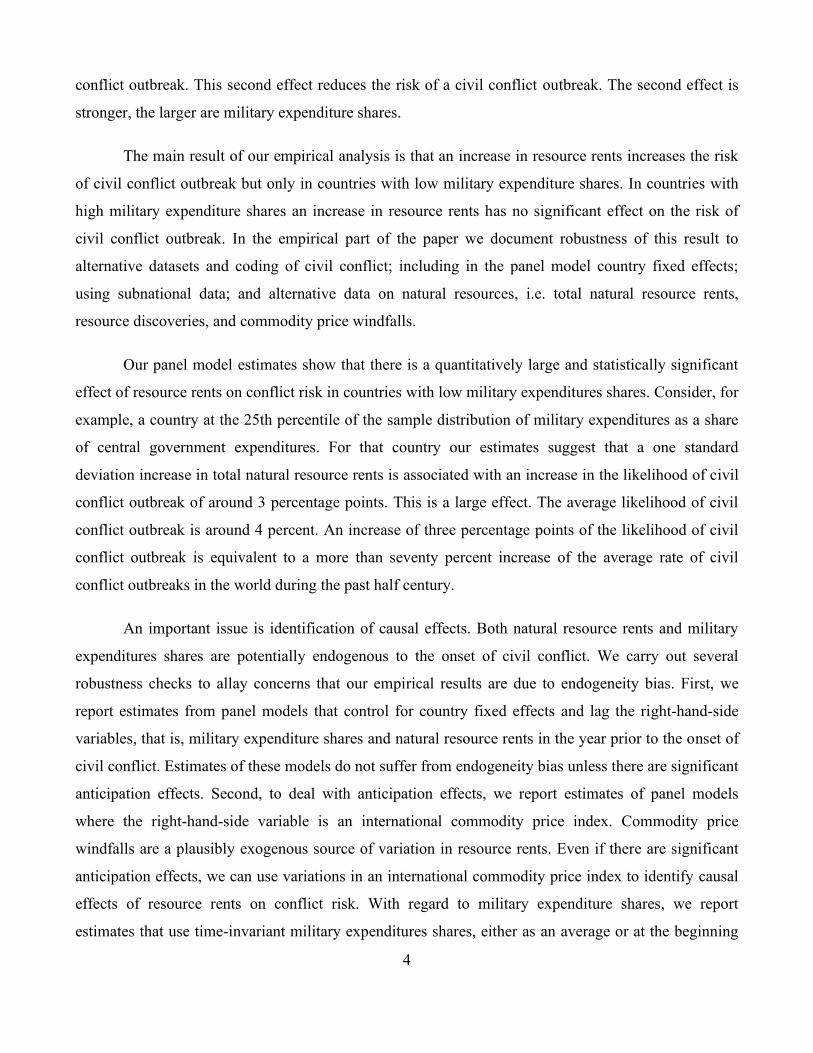
conflict outbreak. This second effect reduces the risk of a civil conflict outbreak. The second effect is

stronger, the larger are military expenditure shares.

The main result of our empirical analysis is that an increase in resource rents increases the risk

of civil conflict outbreak but only in countries with low military expenditure shares. In countries with

high military expenditure shares an increase in resource rents has no significant effect on the risk of

civil conflict outbreak. In the empirical part of the paper we document robustness of this result to

alternative datasets and coding of civil conflict; including in the panel model country fixed effects;

using subnational data; and alternative data on natural resources, i.e. total natural resource rents,

resource discoveries, and commodity price windfalls.

Our panel model estimates show that there is a quantitatively large and statistically significant

effect of resource rents on conflict risk in countries with low military expenditures shares. Consider, for

example, a country at the 25th percentile of the sample distribution of military expenditures as a share

of central government expenditures. For that country our estimates suggest that a one standard

deviation increase in total natural resource rents is associated with an increase in the likelihood of civil

conflict outbreak of around 3 percentage points. This is a large effect. The average likelihood of civil

conflict outbreak is around 4 percent. An increase of three percentage points of the likelihood of civil

conflict outbreak is equivalent to a more than seventy percent increase of the average rate of civil

conflict outbreaks in the world during the past half century.

An important issue is identification of causal effects. Both natural resource rents and military

expenditures shares are potentially endogenous to the onset of civil conflict. We carry out several

robustness checks to allay concerns that our empirical results are due to endogeneity bias. First, we

report estimates from panel models that control for country fixed effects and lag the right-hand-side

variables, that is, military expenditure shares and natural resource rents in the year prior to the onset of

civil conflict. Estimates of these models do not suffer from endogeneity bias unless there are significant

anticipation effects. Second, to deal with anticipation effects, we report estimates of panel models

where the right-hand-side variable is an international commodity price index. Commodity price

windfalls are a plausibly exogenous source of variation in resource rents. Even if there are significant

anticipation effects, we can use variations in an international commodity price index to identify causal

effects of resource rents on conflict risk. With regard to military expenditure shares, we report

estimates that use time-invariant military expenditures shares, either as an average or at the beginning

5

of the sample period. These variables are by construction exogenous to the onset of civil conflict in any

particular year.

Larger military expenditure shares reduce the risk of conflict outbreak when a country

experiences an increase in resource rents, but there is a trade-off. Our panel model estimates show that

the larger are military expenditure shares, the smaller is the effect of resource rents on GDP per capita

growth and countries' polity scores. The panel model estimates show that only in countries with low

military expenditure shares does an increase in resource rents have a significant positive effect on GDP

per capita growth and polity scores. We refer to this as the democracy and development dividend of

natural resources. Regarding channels through which this democracy and development dividend of

natural resources materializes: We first inspect the standard channel, namely, saving and investment for

economic growth as suggested by the basic neoclassical growth model, e.g. the Solow-Swan model;

and education for democracy as suggested by the modernization hypothesis. Our panel model estimates

show that in countries with low military expenditure shares an increase in resource rents leads to a

significant increase in the domestic saving rate, the domestic investment rate, public education

expenditures, and school enrollment rates; and there is a decrease in poverty rates and poverty gaps.

This is hence the trade-off: in countries with high military expenditure shares there is no

conflict resource curse – and, there is also no democracy and development dividend. We believe this

trade-off is plausible. The larger is the military expenditure share the smaller is the share of resources

that government allocates on public goods, such as public education, that enhance the average human

capital of the population.

The rest of the paper is organized as follows. Section 2 provides a theoretical framework that

suggests that the effect of resource rents on conflict depends on military expenditure shares. Section 3

discusses the empirical results. This section contains three sub-sections. In Section 3.1.1 we discuss

estimates of panel models where the right-hand-side variable is total natural resource rents. Variations

in total natural resources rents are affected by the variation in the international prices of the natural

resources and the quantity produced in each country. Since the outbreak of civil conflict in a country

might affect resource production in that country, variations in total natural resource rents are not

plausibly exogenous. The results in Section 3.1.1 can thus only be interpreted as a correlation – and not

as a causal relationship – between resource rents and the risk of civil conflict.

6

We report in Section 3.1.2 results for an international commodity price index. As most

countries are price takers on the international commodity market, the estimates in Section 3.1.2 are

plausibly reflecting a causal effect of international commodity price windfalls on civil conflict. The

effects of increased wealth in commodity-exporting countries on civil conflict risk that is due to

international commodity price booms may or may not be the same as the effects that resource wealth

has on civil conflict that is due to the discovery or changes in the produced quantity of the natural

resource. We report in Section 3.1.3 results for oil reserves and discoveries, using existing methods in

the literature to establish a causal effect of these variables on civil conflict. Section 3.2 discusses

estimates of the effects that resource rents have on democracy and economic growth. Section 4

concludes.

2. A Simple Theoretical Framework

This section contains a simple theoretical framework. The purpose of the model developed here is to

formalize our argument that the effect of resource rents on conflict depends on military expenditure

shares. The theoretical framework is motivated by Azam (1995), Grossman (1995), Hirshleifer (1995)

and Collier and Hoeffler (1998)5.

The starting point is the assumption that rebels maximize the expected net gain from rebellion:

expected revenue (ER) – costs (C). The likelihood of a conflict outbreak, L(Conflict), depends on the

economic incentives for rebellion:

(1) L(Conflict) = f(net gain from rebellion)=f(ER, C); dL(Conflict)/dER > 0

(2) Expected Revenue (ER) = probability of successful rebellion (p)* revenue captured (T)

where p is a decreasing function of military expenditures:

(3) ER = p(M)*T with dp/dM < 0

Revenues can be used by the government to finance the military, or they can be allocated for

something else. Thus, we now write that p(M(T)), where M is military expenditure and T is revenues.

(4) ER = p(M(T))*T

5 See also Dal Bo and Dal Bo (2011), Acemoglu et al. (2011), or Chassang and Padro-i-Miquel (2014).

7

The simplest relationship is where:

(i) military expenditures are a constant fraction, a, of revenues, T, so that M=aT; and

(ii) the probability of successful rebellion is decreasing in military expenditures:

(5) p(M(T)) = 1- aT

where M, T, and a are normalized on the unit interval. This yields

(6) ER= (1- aT)T

Differentiating expected revenues with respect to T one obtains the following marginal effect:

(7) d(ER)/dT= 1-2*aT

which is strictly decreasing in a, the share of revenues allocated to military expenditures.6

In the empirical analysis, we will begin by using military expenditures as a share of central

government expenditures. This variable corresponds one-to-one to the a in the theoretical framework

development above. More data (about twice as many country-year observations) are available for

military expenditures as a share of GDP than for military expenditures as a share of central government

expenditures. In order to maximize observations, we will report in subsequent tables results that use

military expenditures as a share of GDP. Military expenditures as a share of central government

expenditures are positively correlated with the GDP share of military expenditures (correlation

coefficient is around 0.69). That is, countries with a large GDP share of military expenditures also tend

to have a large share of military expenditures in central government expenditures.

3. Empirical Results

3.1. Natural Resources and Civil Conflict

3.1.1. Total Natural Resource Rents

3.1.1.1 Estimates of an Interaction Model with Countries' Average Military Expenditures as a Share of

Central Government Expenditures

6 In their empirical analysis Collier and Hoeffler use natural resource endowments as a proxy for T. One could further fine

tune the model by assuming that government receives a constant fraction, φ, of the resource rents, R, so that dT=φdR.

8

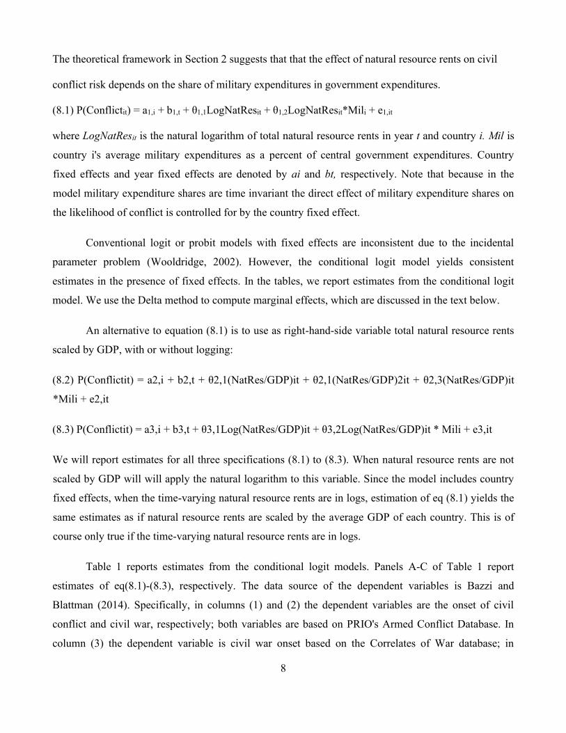
The theoretical framework in Section 2 suggests that that the effect of natural resource rents on civil

conflict risk depends on the share of military expenditures in government expenditures.

(8.1) P(Conflictit) = a1,i + b1,t + θ1,1LogNatResit + θ1,2LogNatResit*Mili + e1,it

where LogNatResit is the natural logarithm of total natural resource rents in year t and country i. Mil is

country i's average military expenditures as a percent of central government expenditures. Country

fixed effects and year fixed effects are denoted by ai and bt, respectively. Note that because in the

model military expenditure shares are time invariant the direct effect of military expenditure shares on

the likelihood of conflict is controlled for by the country fixed effect.

Conventional logit or probit models with fixed effects are inconsistent due to the incidental

parameter problem (Wooldridge, 2002). However, the conditional logit model yields consistent

estimates in the presence of fixed effects. In the tables, we report estimates from the conditional logit

model. We use the Delta method to compute marginal effects, which are discussed in the text below.

An alternative to equation (8.1) is to use as right-hand-side variable total natural resource rents

scaled by GDP, with or without logging:

(8.2) P(Conflictit) = a2,i + b2,t + θ2,1(NatRes/GDP)it + θ2,1(NatRes/GDP)2it + θ2,3(NatRes/GDP)it

*Mili + e2,it

(8.3) P(Conflictit) = a3,i + b3,t + θ3,1Log(NatRes/GDP)it + θ3,2Log(NatRes/GDP)it * Mili + e3,it

We will report estimates for all three specifications (8.1) to (8.3). When natural resource rents are not

scaled by GDP will will apply the natural logarithm to this variable. Since the model includes country

fixed effects, when the time-varying natural resource rents are in logs, estimation of eq (8.1) yields the

same estimates as if natural resource rents are scaled by the average GDP of each country. This is of

course only true if the time-varying natural resource rents are in logs.

Table 1 reports estimates from the conditional logit models. Panels A-C of Table 1 report

estimates of eq(8.1)-(8.3), respectively. The data source of the dependent variables is Bazzi and

Blattman (2014). Specifically, in columns (1) and (2) the dependent variables are the onset of civil

conflict and civil war, respectively; both variables are based on PRIO's Armed Conflict Database. In

column (3) the dependent variable is civil war onset based on the Correlates of War database; in

9

column (4) the dependent variable is civil war onset from Collier and Hoeffler (2004). The data source

of the right-hand-side variables is World Bank (20187).

In Panel A one can see that the coefficient on the log of natural resource rents is positive and

the coefficient on the interaction between the log of natural resource rents and the share of military

expenditures is negative. Both coefficients are individually significantly different from zero at the

conventional significance levels. The interpretation of the estimates in Panel A of Table 1 is that an

increase in natural resource rents is associated with an increase in the likelihood of civil conflict

outbreak -- but less so the higher is the share of military expenditures in central government

expenditures.

Military expenditure shares have a substantial effect on the relationship between conflict risk

and resource rents. Take, for example, the estimated coefficients in column (1) of Panel A in Table 1.

Applying the Delta method to obtain marginal effects from the conditional logit model and

differentiating with respect to the log of total natural resource rents yields:

(8.4) dP(Conflict)/dLogNatres = 1.55 – 0.05*Mil

According to the above equation, if the share of military expenditures in central government

expenditures is equal to zero (Mil=0) then a 1 log increase in total resource rents is associated with an

increase in the likelihood of conflict outbreak of around one and a half percentage points. For a share

of military expenditures in central government expenditures equal to thirty percent (Mil=30), the effect

of a 1 log increase in total resource rents on the likelihood of conflict outbreak is zero after rounding to

the first decimal.

The estimates in Table 1 suggest that in countries with a low share of military expenditures in

central government expenditures, an increase in natural resource rents leads to a large increase in the

likelihood of civil conflict outbreak. Consider, for example, a country at the 25th percentile of the

sample distribution of the share of military expenditures in central government expenditures.

According to the estimates in Panel A of Table 1, a one standard deviation increase in the log of natural

7 In Table 1 the panel spans the period 1970-2007; this is the longest period given the available conflict data from Bazzi and

Blattman and data on natural resource rents and military expenditures from the World Development Indicators. In table 2

and following tables we will use data for a larger and longer panel. This larger and longer panel is based on conflict data

from PRIO (2017) and as right-hand-side variable for the interaction term the average GDP share of military expenditures.

10

resource rents is associated with an increase in the likelihood of civil conflict outbreak of around 3

percentage points; for civil war outbreak the effect is even larger, around 5 percentage points.

To contrast the above effect to a country with a relatively high military expenditure share,

consider now a country at the 75th percentile of military expenditures in central government

expenditures. For that country, the effects of resource rents on conflict risk are about half as large as at

the 25th percentile. Statistically, the effects are much weaker. At the 75th percentile only for civil

conflict onset, i.e. column (1), can one reject that the effect of resource rents on civil conflict onset is

equal to zero at the 10 percent significance level (p-value 0.07). For all three measures of civil war

onset, i.e. columns (2)-(4), one cannot reject the null that the effect is equal to zero at the conventional

significance levels.

Our main finding, that the effect of resource rents on conflict onset risk is declining in military

expenditures continues to hold for alternative functional forms. Panel B of Table 1 shows estimates if

the right-hand-side variable is the GDP share of total natural resource rents and its square. From Panel

B one can see that the estimated coefficient on the GDP share of natural resource rents is positive while

the coefficient on the squared GDP share of natural resource rents is negative.8 Similar to Panel A, the

coefficient on the interaction between the GDP share of natural resource rents and countries' average

shares of military expenditures in central government expenditures are negative. Panel C of Table 1

shows that this is also the case if the squared term of the GDP share of military expenditures is not

included in the model.

3.1.1.2 Estimates of Interaction Models with Military Expenditures as a Share of GDP Time-Varying

Table 2 shows estimates of models where the log of the GDP share of natural resource rents of country

i in year t is interacted with the log of the GDP share of military expenditures of country i in year t.9

8 The same result was obtained in the previous literature, see e.g. Collier and Hoeffler, 1999. Specifically in Panel B of

Table 1 the estimates can be interpreted as follows. At higher levels of GDP shares of natural resource rents, an additional

percentage point increase in the GDP share of natural resource rents has smaller effects on conflict risk than at lower GDP

share of natural resource rents, i.e. there are diminishing effects. If one plots the relationship between

9 In Table 1 natural resource rents of country i in period t are interacted with country i's average military expenditures as a

share of central government expenditures. There are about twice as many country-year observations for the GDP share of

military expenditures as for the GDP share of central government expenditures. Note that the theoretical framework in

Section 2 is based on military expenditures as a share of central government expenditures. There is hence a trade-off: we

have more statistical power when using the GDP share of military expenditures but the theoretical framework is based on

military expenditures as a share of central government expenditures. Military expenditures as a share of central government

11

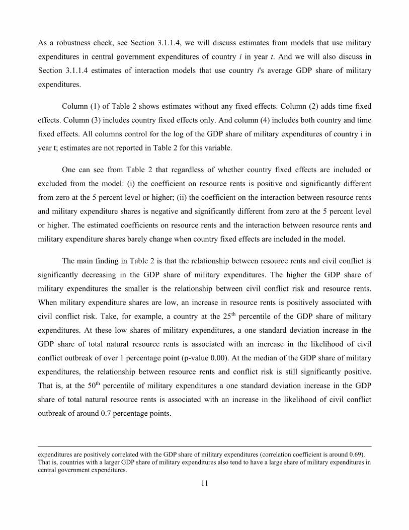
As a robustness check, see Section 3.1.1.4, we will discuss estimates from models that use military

expenditures in central government expenditures of country i in year t. And we will also discuss in

Section 3.1.1.4 estimates of interaction models that use country i's average GDP share of military

expenditures.

Column (1) of Table 2 shows estimates without any fixed effects. Column (2) adds time fixed

effects. Column (3) includes country fixed effects only. And column (4) includes both country and time

fixed effects. All columns control for the log of the GDP share of military expenditures of country i in

year t; estimates are not reported in Table 2 for this variable.

One can see from Table 2 that regardless of whether country fixed effects are included or

excluded from the model: (i) the coefficient on resource rents is positive and significantly different

from zero at the 5 percent level or higher; (ii) the coefficient on the interaction between resource rents

and military expenditure shares is negative and significantly different from zero at the 5 percent level

or higher. The estimated coefficients on resource rents and the interaction between resource rents and

military expenditure shares barely change when country fixed effects are included in the model.

The main finding in Table 2 is that the relationship between resource rents and civil conflict is

significantly decreasing in the GDP share of military expenditures. The higher the GDP share of

military expenditures the smaller is the relationship between civil conflict risk and resource rents.

When military expenditure shares are low, an increase in resource rents is positively associated with

civil conflict risk. Take, for example, a country at the 25th percentile of the GDP share of military

expenditures. At these low shares of military expenditures, a one standard deviation increase in the

GDP share of total natural resource rents is associated with an increase in the likelihood of civil

conflict outbreak of over 1 percentage point (p-value 0.00). At the median of the GDP share of military

expenditures, the relationship between resource rents and conflict risk is still significantly positive.

That is, at the 50th percentile of military expenditures a one standard deviation increase in the GDP

share of total natural resource rents is associated with an increase in the likelihood of civil conflict

outbreak of around 0.7 percentage points.

expenditures are positively correlated with the GDP share of military expenditures (correlation coefficient is around 0.69).

That is, countries with a larger GDP share of military expenditures also tend to have a large share of military expenditures in

central government expenditures.

12

Figure 1 illustrates graphically how the relationship between resource rents and the likelihood

of conflict outbreak depends on the GDP share of military expenditures. The figure is based on the

estimates in column (1) of Table 2. On the y-axis of Figure 1 is the effect of a 1-log increase in the

GDP share of total natural resource rents on the likelihood of civil conflict onset. The dashed lines are

95 percent confidence bands. One can see that for low military expenditure shares, i.e. below 2 percent

of GDP, there is a significant positive relationship between resource rents and conflict risk. Above 2

percent of military expenditures in GDP there is no significant effect of resource rents on conflict

outbreak risk.

3.1.1.3 Sample Split

Appendix Table 3 shows estimates of econometric models where the dependent variable is civil

conflict onset and the right-hand-side variable is the log of total natural resource rents as a share of

GDP. Panel A (B) reports estimates for the sub-sample of country-years with low and intermediate

(high) military expenditures, i.e. where military expenditures are below (above) 3.3% of GDP; this is

the 75th percentile.

Column (1) shows estimates from a simple bivariate logit model. One can see that the estimated

coefficient on resource rents is significantly positive in the sub-sample with low and intermediate

military expenditure shares, but significantly negative in the sub-sample with high military

expenditures. Column (2) shows that these estimates do not change substantially if time fixed effects

are included on the right-hand side of the estimating equation. After computing the marginal effects,

these estimates mean that a one standard deviation increase in the GDP share of natural resource rents

is associated with an increase in the likelihood of civil conflict outbreak of around 1.3 percentage

points, on average, in the subset of countries with low and intermediate military expenditure shares. In

countries with high military expenditure shares, a one standard deviation increase in natural resource

rents is associated with a decrease in the likelihood of civil conflict outbreak of around 1.1 percentage

points.

Columns (3) and (4) show estimates from conditional logit models with country fixed effects.

The within-country estimates show a positive coefficient on resource rents in the sample of countries

with low and intermediate military expenditures shares. Including country fixed effects leads to a

substantial increase (i.e. more than doubling) in standard errors. Only in column (4), for the sample of

13

countries with low and intermediate military expenditure shares, when both time and country fixed

effects are included in the model can one reject the null hypothesis that the coefficient on resource rents

is equal to zero at the 10 percent significance level. For the sample of countries with high military

expenditure shares the estimated coefficient on resource rents is not significantly different from zero.

The estimates from econometric models where the sample is split are easy to interpret, however,

this is not the most efficient method for estimating how military expenditure shares affect the

relationship between resource rents and civil conflict risk. Estimation of an interaction model that

includes an interaction term between resource rents and military expenditure shares is more efficient.

The interaction model also enables to provide estimates of the relationship between resource rents and

conflict for specific values of military expenditure shares. This is why the baseline estimates and

robustness tests are for an interaction model, rather than for a model where the sample is split at certain

thresholds of military expenditure shares.

3.1.1.4 Robustness

This section discusses robustness of the interaction model to:

• alternative functional forms

• not scaling resource rents by GDP;

• using military expenditures scaled by central government expenditures;

• excluding from the sample observations with extremely low GDP shares of resource

rents or GDP shares of military expenditures;

• controlling for lagged civil conflict;

• using time-invariant measures of military expenditure shares, i.e. countries' average

or beginning of sample military expenditure shares

• alternative civil war onset datasets;

• estimation of the model for the sub-set of countries in the Middle East and North

Africa.

14

Alternative Functional Forms and Scaling

Table 3 documents robustness to alternative functional forms and scaling. In Table 2 both the GDP

share of military expenditures and the GDP share of natural resource rents are in logs. Taking logs

means that larger values, i.e. higher percentages of the GDP shares of military expenditures and

resource rents are given less weight. Table 3 shows that, qualitatively, we obtain similar results if we

do not take logs of the right-hand side variables: When the GDP share of military expenditures is low,

a higher GDP share of resources rents is associated with a significantly higher risk of civil conflict.

Take, for example, a country at the 25th percentile of the GDP share of military expenditures. At this

relatively low GDP share of military expenditures, the estimates in Table 3 suggest that a 1 standard

deviation (11 percentage points) increase in the GDP share of resource rents is associated with an

increase in the likelihood of civil conflict outbreak of around 0.7 percentage points. At the 50th

percentile of the GDP share of military expenditures a 1 standard deviation increase in the GDP share

of resource rents is associated with an increase in the likelihood of civil conflict of around 0.4

percentage points.

Not Scaling Resource Rents by GDP

Table 4 shows estimates of models where we use as right-hand-side variable the log of total natural

resource rents – i.e. resource rents are not scaled by GDP. Table 4 shows that our main result is still

intact: In countries with a low GDP share of military expenditures, total natural resource rents are

positively associated with conflict risk. The higher the GDP share of military expenditures, the less

likely it is that an increase in resource rents is associated with an outbreak of conflict. Take, for

example, a country at the 25th percentile of the GDP share of military expenditures. At this relatively

low GDP share of military expenditures, the estimates in Table 4 suggest that a 1 standard deviation

increase in the log of total natural resource rents is associated with an increase in the likelihood of civil

conflict outbreak of around 1 percentage point (p-value 0.00). At the 90th percentile of the GDP share

of military expenditures, the connection between resource rents and conflict is much weaker and not

significantly different from zero. According to the estimates in Table 4, at the 90th percentile of the

GDP share of military expenditures, a 1 standard deviation increase in the log of total natural resource

rents is associated with an increase in the likelihood of civil conflict outbreak of around 0.2 percentage

points (p-value 0.39).

15

Military Expenditures as a Share of Central Government Expenditures Time-Varying

Table 5 reports results if we estimate the interaction model with military expenditures scaled by central

government expenditures of country i in year t. The estimates in Table 5 show that in countries with a

low share of military expenditures in central government expenditures, resource rents are positively

associated with conflict risk. The higher the share of military expenditures in central government

expenditures, the less likely it is that an increase in resource rents is associated with an outbreak of

conflict. Take, for example, a country at the 25th percentile of the share of military expenditures in

central government expenditures. At this relatively low share of military expenditures in central

government expenditures, the estimates in Table 5 show that a 1 standard deviation increase in the

GDP share of total natural resource rents is associated with an increase in the likelihood of civil

conflict outbreak of over 2 percentage points (p-value 0.00). At the 90th percentile of the share of

military expenditures in central government expenditures, the connection between resource rents and

conflict is much weaker and not significantly different from zero. According to the estimates in Table

5, at the 90th percentile of the share of military expenditures in central government expenditures, a 1

standard deviation increase in the GDP share of total natural resource rents is associated with an

increase in the likelihood of civil conflict outbreak of around 0.3 percentage points (p-value 0.33).

Excluding Low GDP Shares of Resource Rents or Low GDP Shares of Military Expenditures

Table 6 shows that results are robust to excluding the bottom 10th percentile of GDP shares of natural

resource rents (Panel A) or the bottom 10th percentile of GDP shares of military expenditures (Panel

B). Relative to the estimates in Table 2, one can see that the estimated coefficients in Table 6 are in

absolute size somewhat larger. This is true both for the estimated coefficient on the log of the GDP

share of resource rents and for the estimated coefficient on the interaction of that variable with the

GDP share of military expenditures.

Controlling for Lagged Conflict

Table 7 reports estimates when adding to the right-hand side of the estimating equation the lagged

dependent variable. Comparing the estimates in Table 7 to the estimates in Table 2 one can see that

adding the lagged dependent variable does not substantially change the estimated coefficients on

resource rents and the interaction between resource rents and military expenditures. In the models

without country fixed effects, see columns (1) and (2), the estimated coefficient on the lagged

dependent variable is positive and significantly different from zero at the conventional significance

16

levels. In models that include country fixed effects, see columns (3) and (4), the estimated coefficient

on the lagged dependent variable is positive but not significantly different from zero at the

conventional significance levels. Regardless of whether country fixed effects are included in the model

or not, one can see in Table 7 that the estimated coefficient on resource rents is significantly positive

while the coefficient on the interaction between resource rents and military expenditures is

significantly negative.

Countries' Average or Beginning of Sample Military Expenditures

In Table 8 we report estimates from models with country fixed effects where military expenditures as a

share of GDP are time-invariant, interacted with the time-varying t-1 GDP shares of total natural

resource rents. An advantage of using time-invariant GDP shares of military expenditures, as opposed

to time-varying GDP shares of military expenditures, is that measurement error of the country average

is typically smaller than the time-varying series; or stated differently, that the cross-country signal to

noise ratio is higher than the within-country signal to noise ratio. Thus, attenuation bias is likely to be

smaller when using time-invariant GDP shares of military expenditures. Using time invariant military

expenditures also means that, by construction, the outbreak of civil conflict in year t does not affect the

GDP share of military expenditures in that year.

In a model with country fixed effects one can estimate the coefficient on the interaction

between time-varying t-1 resource rents and time-invariant military expenditures as a share of GDP.

The direct effect of the time-invariant military expenditures are controlled for by the country fixed

effects. Hence we do not include time-invariant military expenditures on the right-hand side of the

estimating equation in the fixed effects model.

We consider two alternatives for constructing time-invariant military expenditure shares. The

first approach is to generate, for each country, the unweighted average of the GDP share of military

expenditures during 1960-2017. The second approach is to use for each country the GDP share of

military expenditures at the beginning of the sample period. In the 1960s the cross-country data on

military expenditures is very sparse. We thus estimate the sample on the 1971-2017 period, and use the

1970 GDP share of military expenditures for the interaction term for the second approach.

From Table 8 one can see that the correlation between resource rents and the likelihood of civil

conflict outbreak is significantly decreasing in time-invariant measures of countries' GDP shares of

17

military expenditures. Columns (1) and (2) show estimation results where the time-invariant measure is

the country average GDP share of military expenditures; columns (3) and (4) show estimation results

for the beginning of sample GDP shares of military expenditures. Comparing to Table 2, one can see

that the estimated coefficients in Table 8 on resource rents and the interaction with military

expenditures are similar in size and statistical significance.

Alternative Civil Conflict and Civil War Datasets

Bazzi and Blattman (2014) is a recently published paper that contains an empirical analysis of cross-

country civil conflict data. In Table 9 we show estimation results that use as dependent variables the

civil conflict and civil war onset variables of the Bazzi and Blattman (2014) dataset. In columns (1) and

(2) of Table 9 the dependent variables are the PRIO based civil conflict onset and civil war onset

indicator variables, respectively. The civil conflict and civil war onset data are computed by Bazzi and

Blattman based on the PRIO (2011) Armed Conflict Dataset. The key difference between civil conflict

and civil war according to PRIO is the battle death threshold: for civil conflict the threshold is 25 battle

deaths per year, for civil war it is 1000 battle deaths per year. In column (3) the dependent variable is

civil war onset from the Correlates of War (2011). In column (4) the dependent variable is civil war

onset from Collier and Hoeffler (2004). One can see that in all four columns of Table 9 the estimated

coefficient on the t-1 log of the GDP share of natural resource rents is positive and significantly

different from zero at the conventional significance levels. The coefficient on the interaction between

the t-1 log of the GDP share of natural resource rents and countries' average GDP shares of military

expenditures is significantly negative. Noteworthy is that when the dependent variable is civil war

onset the estimated coefficients on the right-hand side variables are somewhat larger in absolute value

than when the dependent variable is civil conflict onset.

MENA

Table 10 shows estimates of the econometric model for the sub-set of countries in the Middle East and

North Africa. Columns (1) and (2) show estimates for an interaction model where countries' t-1 GDP

shares of natural resource rents are interacted with countries' average GDP shares of military

expenditures; in columns (3) and (4) countries' t-1 GDP shares of natural resource rents are interacted

with countries' beginning of sample GDP shares of military expenditures. One can see that the

estimated coefficient on the interaction term is significantly negative while the coefficient on the t-1

GDP share of natural resource rents is positive. Thus, the model predicts that in a MENA country with

18

a low GDP share of military expenditures, an increase in natural resource rents will significantly

increase the risk of civil conflict outbreak; but there is no significant effect on the risk of civil conflict

outbreak in a country with a high GDP share of military expenditures.

An interesting stylized fact about MENA is that the average GDP share of total natural resource

rents is much larger than in other regions of the world – yet, despite this, the average risk of civil

conflict outbreak in MENA is not higher than in the rest of the world. An explanation for this, which is

consistent with the results of the econometric analysis is that, in MENA, the average GDP share of

military expenditures is much larger than in the rest of the world. Thus, in the average MENA country,

rebel's have relatively more to gain (from appropriating the natural resources) but their success

probability is also relatively low (due to a relatively strong military). According to data from the World

Development Indicators and PRIO, during 1960-2017:

1. The average GDP share of total natural resource rents in MENA was around 15

percent. This is more than three times the average GDP share of total natural resource

rents in the rest of the world.

2. The average likelihood of civil conflict (civil war) outbreak in MENA was around

three (two) percent while in the rest the world the average likelihood of civil conflict

(civil war) outbreak was around four (two) percent.

3. The average GDP share of military expenditures in MENA was around 7 percent; in

the rest of the world the average GDP share of military expenditures was around 2

percent.

3.1.2. Commodity Price Windfalls

In this section we report estimates of the impact that international commodity price windfalls have on

the risk of civil conflict outbreak. Section 3.1.2.1 shows panel model estimates of cross-country time-

series data. Our main variable for the cross-country analysis is an international commodity price index

where the international commodity prices are geometrically weighted with countries' average GDP

shares of the export values of the commodities; the index is constructed in the same way as in Arezki

19

and Brueckner (2012). Ciccone (2019) uses as weights countries' average export shares in total exports;

we will discuss results using the Ciccone data as a robustness check in Section 3.1.2.1. In Section

3.1.2.2 we will show estimates of econometric models that are based on subnational data of sub-

Saharan African countries. In that section we will use the dataset and estimation methods of Berman et

al. (2017).

3.1.2.1 Cross-Country Time Series Regressions

Table 11 shows conditional logit fixed estimates of the effects that windfalls from international

commodity price booms have on the risk of civil conflict outbreak. The unbalanced panel covers more

than 150 countries and spans the period 1960-2017. The econometric model includes country and time

fixed effects. The commodity price index enters in year t-1 and is interacted with countries' average

GDP shares of military expenditures.

The four columns of Table 11 show estimates for different commodities that are included in the

commodity price index. In column (1) the price index includes gas and oil only. In column (2) the

index includes all capital-intensive commodities, i.e. gas and oil, as well as minerals and metals.

Column (3) reports estimates for a commodity price index that includes agricultural commodities only.

Column (4) reports estimates for an index that includes all commodities.

As argued, for example, in Dube and Vargas (2013) price shocks to capital-intensive

commodities have different effects on the risk of civil conflict outbreak than labor-intensive

commodities. For a commodity exporting country, an increase in the international price of capital-

intensive commodities increases rents (relative to wages); an increase in the international price of

labor-intensive commodities increases wages (relative to rents). This is the Stolper-Samuelson

Theorem.

With regard to conflict risk, we already pointed out in Section 2 that the incentives for rebellion

are determined by expected rents relative to costs. We only discussed there expected rents but here it is

appropriate to also discuss costs. Rebels need to recruit militia. That is, rebels have to trade off the

wage earned in the labor market to that what they expect to gain from rebellion. When wages rise

relative to rents the value of rents captured from successful rebellion decrease relative to costs. And

vice versa. Hence, an increase in international prices of capital-intensive goods increase conflict risk

while the opposite is the case for labor-intensive goods. However, regardless of whether commodities

20

are capital intensive or labor intensive, a better financed military decreases the success probability of

rebellion. And thus, an increase in international commodity prices has a smaller effect on expected

rents the greater are military expenditures. This is true for both capital-intensive and labor-intensive

commodities.

The estimates in Table 11 show that the effect of commodity price windfalls on civil conflict

risk is decreasing in the GDP share of military expenditures. Consider, for example, the estimates in

column (1) which are for a commodity price index that includes oil and gas only. The estimated

coefficient on the t-1 commodity price index is positive and significantly different from zero at the 1

percent level. The estimated coefficient on the interaction between the t-1 commodity price index and

countries' average GDP shares of military expenditures is negative and significantly different from zero

at the1 percent level. To have an understanding of the size of the effect, let us consider various

percentiles of the sample distribution of countries' average GDP shares of military expenditures. At the

25th percentile of the GDP share of military expenditures, a one standard deviation increase in the

commodity price index that includes oil and gas only increases the risk of civil conflict outbreak in the

next year by around 10 percentage points. This effect is significantly different from zero at the 5

percent level. At the 50th and 75th percentile of the GDP share of military expenditures, a one standard

deviation increase in the commodity price index that includes oil and gas only increases the risk of civil

conflict outbreak in the next year by around 7 and 4 percentage points, respectively. These effects are

significantly different from zero at the 5 percent level and 10 percent level, respectively. At the 90th

percentile of GDP share of military expenditures, the effect is quantitatively small and not significantly

different from zero at the conventional significance levels. Comparing the estimated coefficients in

column (1) to those in column (2), one can see that they are qualitatively similar, though quantitatively

the coefficients are somewhat smaller in column (2) than in column (1). This suggests that effects are

particularly large for oil and gas.

Windfalls from price booms in agricultural commodities are associated with a decrease in the

risk of civil conflict outbreak, especially in countries with large military expenditure shares. According

to the estimates of column (3) of Table 11, the conflict reducing effect of agricultural commodity price

windfalls is larger in those countries with a higher GDP share of military expenditures. Statistically, the

effect of agricultural commodity price windfalls on conflict risk is different from zero at the

conventional significance levels but only in those countries with a high GDP share of military

21

expenditures. Take, for example, a country at the 75th percentile of the GDP share of military

expenditures: according to column (3) a one standard deviation increase in the agricultural commodity

price index reduces the likelihood of civil conflict outbreak by nearly 5 percentage points. This effect is

significantly different from zero at the 5 percent level. At the 90th percentile of the GDP share of

military expenditures the effect is even larger: a one standard deviation increase in the agricultural

commodity price index reduces the likelihood of civil conflict outbreak by over 7 percentage points. At

low GDP shares of military expenditure the effects are quantitatively smaller and not significantly

different from zero: for example, at the 50th (25th) percentile of the GDP share of military expenditures,

a one standard deviation increase in the agricultural commodity price index reduces the likelihood of

civil conflict outbreak by around 3 (1) percentage points.

Comparing to Dube and Vargas (2013)

Dube and Vargas (2013) present estimates of the effect that commodity price shocks have on civil

conflict risk in Colombia. They find that: (i) an increase in international oil prices increases the

likelihood of conflict in Colombia; (ii) an increase in international agricultural prices decreases conflict

risk. We can use the estimates in Table 11 to compare with the results in Dube and Vargas. That is, we

can compute the predicted effects for a GDP share of military expenditures equivalent to that of

Colombia.

Average military expenditures as a share of GDP were about 2.7 percent in Colombia. Given

this value of military expenditures as a share of GDP, the prediction from the estimates in Table 11 is a

negative relationship between civil conflict risk and agricultural commodity price windfalls and a

significant positive relationship between civil conflict risk and oil price windfalls.

Specifically, for military expenditures equal to the mean in Colombia during the sample at

hand, the prediction from the estimates in Table 11 is that: (i) a one standard deviation increase in the

oil price index increases the likelihood of civil conflict outbreak by around 5.8 percentage points, this

effect is significantly different from zero at the 5 percent significance level (p-value 0.046); (ii) a one

standard deviation increase in the agricultural price index decreases the likelihood of civil conflict

outbreak by around 4 percentage points, this effect is significantly different from zero at the 10 percent

significance level (p-value 0.067).

22

The results in Table 11, that are based on a large cross-country panel are thus consistent with

the subnational estimates in Dube and Vargas for Colombia. For a commodity exporter like Colombia –

which by international comparison has intermediate levels of the GDP share of military expenditures --

an increase in the international price of oil increases the likelihood of a civil conflict outbreak while an

increase in the international price of agricultural commodities decreases the likelihood of conflict.

Alternative Data: Ciccone (2019)

In a recent working paper, Ciccone (2019) presents new evidence of the effect that export price shocks

have on civil war outbreak. One of Ciccone's main points is that, for identifying effects of price shocks,

it is crucial to use commodity price indices that are based on time-invariant export weights. Time-

varying exports weights, as e.g. Bazzi and Blattman (2014) employ in their baseline, do not enable to

distinguish between a price effect and a quantity effect. Another point that Ciccone makes is that

constructing the index based on time-varying exports weights could attenuate estimates towards zero

due to noisily measured time-series data of commodity exports. We agree with both of these points.

In Appendix Table 4, we present estimates that use the Ciccone (2019) data. We also follow

Ciccone's model specification and estimation method. That is, we include country fixed effects,

country-specific linear time trends and year fixed effects as right-hand-side controls. The price shocks

enter in period t, t-1, and t-2. The model is estimated using least squares as in Ciccone (2019).

In column (1) of Appendix Table 4, we show estimates for the largest possible sample. This is a

replication of column (3) of Appendix Table 8 in Ciccone (2019). Ciccone reports in column (3) of

Appendix Table 8 the estimated coefficient on a three year price shock – and the p-values from various

tests that are based on the estimates reported in column (1) of Appendix Table 4 in this paper. The

estimates reported in column (1) of Appendix Table 4 are the coefficients and standard errors on which

the p-values reported in column (3) of Appendix Table 8 in Ciccone (2019) are based.

We are able to exactly replicate Ciccone (2019): One can see from column (1) of Appendix

Table 4 that, on average, there is a significant negative relationship between commodity export price

shocks and civil war outbreak in the Ciccone data. The coefficient on the price shock in period t is

negative and significantly different from zero at the conventional significance levels. The coefficients

on the export price shocks in t-1 and t-2 are also negative but one cannot reject the null that

individually these coefficients are equal to zero.

23

Column (2) of Appendix Table 4 reports estimates for the largest sample for which data on

military expenditure shares are available. One can see that for this sub-sample, the estimated

coefficients on the export price shocks are negative and individually significantly different from zero in

periods t, t-1, and t-2.

Column (3) of Appendix Table 4 shows estimates for the sub-sample where military

expenditures are less than 2 percent of GDP. This sample comprises about half of the observations of

column (2). One can see that for this sub-sample with low military expenditure shares the coefficient

on the export price shock in period t-2 is positive and significantly different from zero at the 10 percent

significance level. The coefficient on the price shocks in period t and t-1 are insignificant.

Column (4) of Appendix Table 4 reports estimates for the same sub-sample as in column (3),

i.e. where military expenditures are less than 2 percent of GDP, but the model includes only country

fixed effects and country-specific linear time trends -- i.e. we do not include year fixed effects.

Excluding year fixed effects leads to somewhat larger estimated coefficients (in absolute value) on the

export price shocks. This is expected since the year fixed effects control for world-wide shocks. In

column (4) of Appendix Table 4 the coefficient on the t-2 price shock is positive and significantly

different from zero at the 5 percent significance level. Quantitatively, the coefficient on the t-2 price

shock in column (4) is about twice as large as the coefficient on the t-2 price shock in column (3).

Column (5) of Appendix Table 4 shows estimates for the sub-sample where military

expenditures exceed 2 percent of GDP. This sample comprises about half of the observations in column

(2). One can see that for this sub-sample with high military expenditure shares the coefficients on the t-

1 and t-2 export price shock are negative and significantly different from zero at the 10 percent

significance level. The coefficient on the price shock in period t is insignificant. In column (6) we

report estimates for the same sub-sample as in column (5) but the model includes only country fixed

effects and country-specific linear time trends -- i.e. we do not include year fixed effects. In that model

specification only the price shock in t-1 is significantly different from zero at the 10 percent level.

The main message of the estimates in columns (3)-(6) of Appendix Table 4 is that in countries

with low military expenditure shares export price shocks tend to increase the risk of civil war outbreak

while in countries with high military expenditures the opposite is the case.

24

How large are these estimated effects? According to the estimates from the models that include

country fixed effects, country-specific linear time trends and year fixed effects, a one standard

deviation increase in the export price index in year t-2 increases the risk of a civil war outbreak in year

t by around 0.2 percentage points for the subset of countries where the GDP share of military

expenditures is below 2 percent. In the subset of countries where the GDP share of military

expenditures exceeds 2 percent, a one standard deviation increase in the export price index in year t-1

decreases the risk of a civil war outbreak in year t by around 1.2 percentage points.

While qualitatively the results obtained with the Ciccone data are similar to what we obtain

with our data, quantitatively it seems as if with the Ciccone data the effects are smaller for the subset of

countries with low military expenditures shares. There is one key difference, however, with regard to

the commodity price index which makes the quantitative comparison not straightforward. We lay out

this difference in the next paragraph.

The index constructed by Ciccone uses as weights exports of a commodity in total exports – and

not exports of a commodity as a share of GDP. This means that the results with the Ciccone data should

be interpreted as a price shock to a particular commodity having a larger effect on civil war in a

country where exports of that commodity are larger as a share of total exports. The share of a

commodity in total exports is inversely related to export diversification (as measured e.g. by a

Herfindahl index). A larger share of a commodity export in total exports could mean that also the share

of a commodity export in GDP is larger, but this must not necessarily be the case. The ratio of

commodity exports in GDP is a measure of how large commodity exports are relative to the total value

added in a country. The share of commodity exports in GDP is a measure of the economic importance

of commodity exports for the entire economy of a country. The share of a specific commodity exported

in total exports is a measure of the economic importance of the commodity exported for a particular

part of a country's economy, namely, the exporting sector.

3.1.2.2 Regressions Using Subnational Data for Africa

The effect of price shocks at the subnational level may differ from the effects at the country level.

Brueckner and Ciccone (2010) found that export price shocks, which increase economic growth, lead

to a significant reduction in the risk of civil war outbreak in sub-Saharan African countries. Their

finding is based on a panel of 39 sub-Saharan African countries during 1980-2009, and an export price

25

index that is generated based on fixed export weights.10 In contrast, using subnational data for Africa,

Berman et al. (2017) found that international commodity price booms increase conflict risk more in

those regions of African countries which produce (more of) that particular commodity. None of these

studies examine how the relationship between commodity price windfalls and conflict risk depends on

military expenditure shares.

Berman et al.'s subnational panel data spans African countries during the 1997-2010 period at a

0.5Ox0.5O spatial resolution. The subnational data enables to examine whether a change in a particular

commodity price has a larger effect on conflict risk in a country's region, i.e. cell, where (more of) that

particular commodity is produced. Berman et al.'s main finding is that, on average, an increase in the

international price of a commodity increases conflict risk more in cells that produce (more of) that

particular commodity. That is, Berman et al. find that on average an increase in resource wealth that is

due to international commodity price booms increases conflict risk at the subnational level.

We first replicate the baseline estimates of Berman et al. (2017) – which are an average effect –

and then examine whether and to what extent the effects differ across sub-Saharan African countries'

military expenditure shares. Column (1) of Appendix Table 5 replicates the estimates of column (1) of

Table 2 in Berman et al. (2017). Referring to equation (1) on page 1573 of Berman et al. (2017), one

can see that the estimate of α3 on ln price mines > 0 is positive and significantly different from zero at

the 5 percent significance level.

Column (2) of Appendix Table 5 shows estimates for the sub-sample for which data are

available on the share of military expenditures in central government expenditures. One can see that for

this sub-sample the coefficient α3 is positive and estimated with a standard error that is about as large

as in column (1) of Appendix Table 5. That is, for the sub-sample for which data on military

expenditure shares are available, one can continue to reject that the effect of mineral price shocks on

subnational conflict risk is, on average, equal to zero at the 5 percent significance level.

Columns (3)-(6) of Appendix Table 5 show that only in countries with relatively low military

expenditures as a share of central government expenditures does an increase in mineral prices have a

10 Ciccone (2019) shows that the result of a zero effect documented by Bazzi and Blattman (2014) is entirely driven by

using an index which is based on time-varying exports weights. Ciccone (2019) shows, using the Bazzi and Blattman data,

that when the price index is based on fixed exports weights, commodity export price shocks have on average a significant

negative effect on civil war risk in sub-Saharan Africa.

26

significant positive effect on subnational conflict risk. Estimates for countries with relatively low

military expenditure shares are shown in columns (3) and (4). Consider the estimates in column (3).

Column (3) shows estimates for countries where military expenditures are less than 8.7 % of central

government expenditures, i.e. the bottom 25th percentile of the sample distribution of military

expenditures as a percent of central government expenditures. One can see in column (3) that the

estimated coefficient, α3, is about 2.1 times the coefficient in column (2). This means that for one-

quarter of African countries – i.e. at the bottom 25th percentile of military expenditure shares – the

effect of mineral price shocks on subnational conflict risk is about twice as large as the effect that

mineral price shocks have on subnational conflict risk in Africa on average.

Column (4) of Appendix Table 5 shows estimates for countries where military expenditures are

less than 11 % of central government expenditures, i.e. the bottom 50th percentile of military

expenditures as a percent of central government expenditures. In column (4) of Appendix Table 5 the

estimated coefficient, α3, is about 20 percent larger than in column (2). This means that for the group of

African countries with the lowest 50th percent of military expenditure shares, the effect of mineral price

shocks on subnational conflict risk is, on average, about 20 percent larger than the effect that mineral

price shocks have on subnational conflict in the average African country.

Estimates for countries with relatively high military expenditure shares are shown in columns

(5) and (6) of Appendix Table 5. Specifically, column (5) shows estimates for countries where military

expenditures exceed 11 % of central government expenditures, i.e. the top 50th percentile of military

expenditures as a percent of central government expenditures. Column (6) shows estimates for

countries where military expenditures exceed 16 % of central government expenditures, the top 25th

percentile. In both columns (5) and (6) the estimated coefficient α3 is negative and not significantly

different from zero. Thus, in countries with high military expenditure shares mineral price shocks do

not significantly affect conflict risk.

In sum: the results in Appendix Table 5 confirm our main result that the effect of commodity

price shocks on conflict risk is decreasing in military expenditure shares.

3.1.3 Oil Reserves and Discoveries

Cotet and Tsui (2013) use a novel data of oil reserves and discoveries, for a world sample of countries

during 1930–2003, to estimate how oil wealth affects civil conflict risk. Cotet and Tsui's main result is

27

that, once country fixed effects are controlled for there is no significant relationship between oil wealth

and conflict risk, on average – and this is true for both democracies and non-democracies.

Columns (1) and (3) of Panel A of Appendix Table 6 replicate the country-fixed estimates

shown in column (5) of Panels A and B of Table 3 in Cotet and Tsui (2013). These estimates are based

on a linear probability model that includes country fixed effects only. In columns (2) and (4) of Panel A

of Appendix Table 6 we show that the estimates in Cotet and Tsui (2013) are robust to controlling for

year fixed effects in addition to country fixed effects. Columns (1) and (2) show results for

democracies, and columns (3) and (4) for non-democracies. One can see that in all four columns of

Panel A of Appendix Table 6, the estimated coefficient on log oil wealth per capita is not significantly

different from zero.

Panel B of Appendix Table 6 shows that in the sub-set of countries with relatively low military

expenditure shares, an increase in oil wealth per capita is associated with a significant increase in civil

conflict risk. In the sample of countries that are coded by Cotet and Tsui as democracies, i.e. columns

(1) and (2), low military expenditure shares refers to the set of countries with average military

expenditures equal or below 1.4 percent of GDP. This sub-sample comprises about one-quarter of the

country-years that are coded by Cotet and Tsui as democracies; or, alternatively, one-tenth of the

country-years of Cotet and Tsui's entire panel. In the sample of countries that are coded by Cotet and

Tsui as non-democracies, i.e. columns (3) and (4), low military expenditure shares refers to the set of

countries with average military expenditures at or below 2 percent of GDP. This sub-sample comprises

nearly one-half of the country-years that are coded by Cotet and Tsui as non-democracies; or,

alternatively, about one-quarter of the country-years of Cotet and Tsui's entire panel.

For democracies with low military expenditure shares, the estimates in columns (1) and (2) of

Panel B of Appendix Table 6 show that an increase in oil wealth per capita equal to one standard

deviation increases the likelihood of civil conflict outbreak by around 3 percentage points.11 In column

(1) of Panel B, the estimated coefficient on log oil wealth per capita is around 0.26 and has a standard

error of 0.15; one can reject that the coefficient is equal to zero at the 10 percent significance level. In

column (2) where both country and time fixed effects are included in the econometric model, the

estimated coefficient on log oil wealth per capita is around 0.33 and has a standard error of around

11 A one standard deviation of log oil wealth per capita in the Cotet and Tsui dataset is around 10. All right-hand side

variables in Cotet and Tsui's dataset are divided by 100.

28

0.14. One can reject that this estimated coefficient is equal to zero at the 5 percent significance level.

Comparing to Panel A, one can see that for the sub-set of democracies with low military expenditure

shares, the effect of oil wealth on civil conflict risk is more than seven times the effect in the average

democracy.

For non-democracies with low military expenditure shares, the estimates in columns (3 and (4)

of Panel B of Appendix Table 6 show that an increase in oil wealth per capita equal to one standard

deviation increases the likelihood of civil conflict outbreak by around 9 to 10 percentage points. In

column (3) of Panel B, the estimated coefficient on log oil wealth per capita is around 0.89 and has a

standard error of 0.42; one can reject that this estimated coefficient is equal to zero at the 5 percent

significance level. In column (4) where both country and time fixed effects are included in the

econometric model, the estimated coefficient on log oil wealth per capita is around 1.0 and has a

standard error of around 0.43. One can reject that this estimated coefficient is equal to zero at the 5

percent significance level.

From the estimates in Appendix Table 6 a number of interesting comparisons can be made: (i)

for the sub-set of democracies with low military expenditure shares, the effect of oil wealth on civil

conflict risk is more than seven times the effect of the average democracy; (ii) for the sub-set of non-

democracies with low military expenditure shares, the effect of oil wealth on civil conflict risk is more

than four times the effect of the average non-democracy; (iii) in non-democracies the effect of oil

wealth on civil conflict risk is at least three times as large as in democracies.

Panel C of Appendix Table 6 shows that for the sub-set of countries with intermediate and high

military expenditure shares oil wealth has no significant effect on civil conflict risk. This is true for

democracies and non-democracies. Quantitatively, the estimated coefficients on log oil wealth per

capita are small and not significantly different from zero at the conventional significance levels. In the

majority of columns in Panel C of Appendix Table 6, the sign of estimated coefficients on log oil

wealth per capita is negative which suggest, that, if anything, an increase in oil wealth per capita is

associated with a reduction in conflict risk in countries with large military expenditure shares.

To summarize: the results in Appendix Table 6 show the effect of oil wealth on conflict risk is

decreasing in military expenditure shares. Only in the subset of countries with low military expenditure

shares does an increase in oil wealth lead to a significant increase in the risk of civil conflict outbreak.

29

Appendix Table 7 shows two-stage least squares estimates. The instrument for the log of oil

wealth per capita is the same as in Cotet and Tsui (2013): out-of-region natural disasters, the log of oil

reserves per capita, and their product. These instruments are relevant in the sense that they yield a

significant first stage effect: the Kleibergen Paap F-statistic is well in excess of the critical values

below which instruments are declared as weak. To facilitate comparison between two-stage least

squares and least squares estimates, Appendix Table 7 is structured in exactly the same way as

Appendix Table 6. As one can see, the two-stage least squares regressions yield coefficients on the log

of oil wealth per capita that are both statistically and quantitatively similar to the least squares

regressions.

3.1.4 Extension: Military Influence on Government

One would expect that the stronger is the influence of the military on government, the larger are

military expenditure shares. Indeed that is what the estimates presented in Appendix Table 8 show. The

variables on military influence on government are from the Database of Political Institutions (World

Bank, 2018b) and Cheibub et al. (2010). The Database of Political Institutions provides two indicator

variables for military influence on government. The first variable is an indicator that is unity if the chief

executive is a military officer; the indicator is zero else. The second variable is an indicator that is unity

if the defense minister is a military officer; this indicator variable is zero else. Cheibub et al. (2010)

provide data for various forms of dictatorship. Based on their dataset we construct an indicator variable

that is unity if the regime is a military dictatorship; the indicator is zero else.

According to the estimates in Appendix Table 8 that control for country fixed effects, there is a

significant positive within-country relationship between military expenditures shares and military

influence on government. According to the estimates in columns 1 and 2 of Appendix Table 8, during

the time period when the chief executive is a military officer the GDP share of military expenditures is

on average about 0.8 percentage points higher relative to the time period when the chief executive is

not a military officer; and the share of military expenditures in central government expenditures is

about 8.0 percentage points higher. During the time period when the defense minister is a military

officer, the GDP share of military expenditures is on average about 0.7 percentage points higher than

during the time period when the defense minister is not a military officer; and the share of military

expenditures in central government expenditures is about 4.7 percentage points higher. See columns (3)

and (4) of Appendix Table 8. And columns (5) and (6) of Appendix Table 8 show that during the time

30

period of military dictatorship the GDP share of military expenditures is on average about 0.3

percentage points higher than during the time period when there is no military dictatorship; and the

share of military expenditures in central government expenditures is about 5.4 percentage points higher.

Appendix Table 9 shows that oil price windfalls increase the risk of civil conflict outbreak only

in the subset of countries with weak military influence on government. Panel A reports estimates for

countries with strong military influence on government; Panel B reports estimates for countries with

weak military influence on government. One can see that only in Panel B are the estimated coefficients

on the international oil price index positive and significantly different from zero at the conventional

significance levels. In Panel A the estimates are quantitatively small and not significantly different from

zero at the 10 percent level or higher. This is true regardless of whether military influence is measured

by an indicator that is unity if the chief executive is a military officer (column (1)); an indicator that is

unity if the defense minister is a military officer (column (2); or an indicator that is unity if the regime

is a military dictatorship (column (3)).

3.2 Effects of Natural Resource Rents on Political Institutions and Economic

Development

In this section we will examine how military expenditure shares affect the impact that natural resource

rents have on political institutions and economic development. This section thus speaks to another,

related strand of the literature on the effects that natural resource rents have on political institutions and

growth. This literature has evolved over time.12 An early contribution by Sachs and Warner (1995)

suggested that countries with large natural resource endowments had slower (transitional) growth

during the 1970s and 1980s. However, Alexeev and Conrad (2009) showed that countries' with more oil

and mineral endowments have higher levels of GDP per capita. Haber and Menaldo's (2012) panel

vector autoregression analysis did not uncover a systematic relationship between resource dependence

and authoritarianism, which is also in line with the cross-country evidence presented in Alexeev and

Conrad. Arezki and Brueckner (2011) showed that only in countries with large state ownership does an

increase in oil rents lead to a significant increase in corruption and a decrease in political rights.

Brueckner et al. (2012) showed that oil price shocks which permanently increase GDP per capita are,

on average, associated with a significant improvement in countries' polity scores. Brueckner and

Gradstein (2016) showed that international oil price windfalls have, on average, a significant positive

12 See, for example, van der Ploeg (2011) for a review of the literature.

31

effect on schooling. The later two papers are consistent with Lipset's (1959) modernization

hypothesis.13

Our main contribution to this literature is to show that only in countries with low military

expenditures shares does an increase in natural resource rents lead to an increase in GDP per capita

growth and an increase in polity scores. There is a democracy and development dividend of resource

wealth in countries with low military expenditures shares. In contrast, in countries where GDP shares

of military expenditures are high an increase in resource rents has no significant effect on GDP per

capita growth and polity scores.

3.2.1. The Democracy Dividend

Table 12 has as dependent variables various measures of political institutions. In column (1) the

dependent variable is the revised and combined polity (polity2) score from the Polity IV database

(2018). Columns (2)-(4) have as dependent variables the sub-scores on political constraints, political

competition, and executive recruitment. In columns (5) and (6) the dependent variables are the

democracy and autocracy scores, respectively. In column (7) the dependent variable is the checks and

balance score from the World Bank's (2018) Database of Political Institutions. One can see from Table

12 that the estimated coefficient on the log of the GDP share of natural resource rents is positive

(except for column (6) where it is negative) while the coefficient on the interaction with the GDP share

of military expenditure is negative (except for column (6) where it is positive). Qualitatively, the

estimates in Table 12 mean that at low GDP shares of military expenditures an increase in natural

resource rents is associated with a significant increase in the polity2 score, the sub-scores on executive

constraints, political competition, and executive recruitment, the democracy score and the checks and

balance score; and a significant decrease in the autocracy score.

Quantitatively, the estimated effects of natural resource rents on political institutions are sizable.

Consider, for example, the estimates in column (1) of Table 12. For a country at the 25th percentile of

GDP share of military expenditures, a 1 standard deviation increase in the GDP share of natural

resource rents increases the polity2 score by around 0.2 standard deviations. This effect is significantly

different from zero at the 5 percent significance level. At the 50th percentile of the GDP share of

13 Resource windfalls must not always be associated with permanently higher GDP per capita. Brueckner and Ciccone

(2011) showed that transitory rainfall shocks induce a negative correlation between GDP per capita and democracy in

agricultural economies.

32

military expenditures, an increase in natural resource rents is also associated with a significant

improvement in the polity2 score, but the effect is smaller, around two-thirds the effect that materializes

at the 25th percentile of the GDP share of military expenditures.

Figure 2 illustrates graphically the relationship between natural resource rents and countries'

polity2 scores across the sample range of the GDP share of military expenditures. One can see that in

countries with a GDP share of military expenditures above 2 percent, the relationship between resource

rents and the polity2 score is not significantly different from zero at the 5 percent level. Below 2

percent it is significantly positive. Resource rents have larger positive effects on the polity score the

smaller is the GDP share of military expenditures.

Thus, in countries with low GDP shares of military expenditures, an increase in resource rents is

associated with a significant increase in countries' polity scores, stronger political constraints and more

political competition, a strengthening of democracy, a decrease in the autocracy score, and a tightening

of checks and balances. This is the democratic dividend of natural resource wealth. But this democratic

dividend does not accrue in countries with a large GDP share of military expenditures.

3.2.2 The Development Dividend

In this section we discuss results on the relationship between resource rents and various measures of

economic development. We begin by discussing estimates of the effects that natural resource rents have

on GDP per capita growth. For that particular outcome variable, we explore one of the standard

channels, namely, investment.14 Part of the rents which are not consumed are saved, and a part of the

domestic saving may be used for domestic investment. For the investment channel we first explore

effects that resource rents have on the accumulation of physical capital. Results are for annual and 5-

year non-overlapping panels. We then turn to schooling. Our main schooling measures are enrollment

rates: in primary and secondary schools. These variables are proxies for investment in human capital.

We examine the response of the GDP share of government consumption and the share of public

education expenditures in total government expenditures to gain an understanding of the role of

government in affecting the impact that resource rents have on investment. We conclude by discussing

14 We do not explore effects on total factor productivity growth. Theoretically, whether natural resource booms lead to

faster or slower long-run growth depends on how the resource wealth is allocated: The literature on long-run growth (see

e.g. Sachs and Warner, 1999) suggests that if the resource wealth is allocated in a way that leads to an expansion (reduction)

of demand in the sector with increasing returns to scale, then growth will increase (decrease). Examining how military

expenditure shares affect the impact that resource rents have on total factor productivity growth and thus long-run growth in

GDP per capita goes beyond the scope of this paper; we leave this for future research.

33

effects on poverty. We show results for poverty rates and poverty gaps at various PPP income

thresholds. The models for schooling and poverty are estimated using 5-year non-overlapping panel

data. Overall, all of the results discussed in this paper should be interpreted as short- to medium-run

relationship between resource rents and development.

Economic Growth

Tables 13 and 14 show estimates of the effects that resource rents have on economic growth, domestic

saving, investment, the GDP share of government consumption. Table 13 shows estimates of models

for annual panel data. The estimates reported in Table 14 are for 5-year non-overlapping panel data.

From column (1) in Tables 13 and 14 one can see that the estimated coefficient on the log of the GDP

share of natural resource rents is positive while the coefficient on the interaction with the GDP share of

military expenditures is negative. These coefficients can be interpreted as follows: the effect of

resource rents on economic growth is decreasing in military expenditure shares; natural resources rents

have a significant positive effect on economic growth but only in countries with low military

expenditure shares.

Quantitatively, the estimated effects of resource rents on economic growth are sizable.

Consider, for example, the estimates in column (1) of Table 13. For a country at the 25th percentile of

the GDP share of military expenditures, a 1 log increase in the GDP share of natural resource rents

increases GDP per capita growth by around 0.9 percentage points per annum. This effect is

significantly different from zero at the 1 percent significance level. At the 50th percentile of the GDP

share of military expenditures, an increase in natural resource rents is also associated with a significant

increase in GDP per capita growth, but the effect is smaller -- around two-thirds the effect that

materializes at the 25th percentile of the GDP share of military expenditures.

Figure 3 illustrates graphically the relationship between natural resource rents and countries'

GDP per capita growth across the sample range of the GDP shares of military expenditures. One can

see that in countries with a GDP share of military expenditures above 2 percent, the relationship

between resource rents and GDP per capita growth is not significantly different from zero at the 5

percent level. Below 2 percent it is significantly positive. Resource rents have a more positive effect on

countries' GDP per capita growth the lower is the GDP share of military expenditures.

34

Physical Capital Accumulation

In the most basic neoclassical growth model, an increase in resource rents can increase transitional

growth if it leads to an increase in domestic investment. Part of the resource income is saved, and part

of the domestic saving is used for domestic investment. We provide evidence on the domestic saving

and investment channel in columns (2) and (3) of Tables 13 and 14. One can see from columns (2) and

(3) that the estimated coefficient on natural resource rents is positive while the coefficient on the

interaction between resource rents and military expenditure shares is negative. These estimates mean

that in countries with low military expenditure shares an increase in resource rents leads to a significant

increase in the domestic saving rate and the domestic investment rate. The effect of resource rents on

the saving and investment rate is decreasing in military expenditure shares. In countries with high

military expenditure shares, resource rents have no significant effect on domestic saving and domestic

investment.

How large are the effects on domestic saving and domestic investment? Consider, for example,

the estimates in columns (2) and (3) of Table 13: For a country at the 25th percentile of the GDP share

of military expenditures, a 1 log increase in the GDP share of natural resource rents increases the

domestic saving rate by 0.09 logs and the domestic investment rate by 0.03 logs. These effects are

significantly different from zero at the 5 and 10 percent significance level, respectively. At the 50th

percentile of the GDP share of military expenditures, an increase in natural resource rents is also

associated with an increase in domestic saving and investment but the effect is smaller -- around two-

thirds the effect that materializes at the 25th percentile of the GDP share of military expenditures.

Column (4) of Tables 13 and 14 shows that one of the reasons for the smaller effect of resource

rents on the domestic saving and investment rates in countries with a larger GDP share of military

expenditures is that, the larger military expenditure shares, the larger is the effect of resource rents on

the GDP share of government consumption. This can be seen from the significant positive coefficients

in column (4) of Tables 13 and 14 on the interaction between the GDP share of resource rents and the

GDP share of military expenditures. The higher the military expenditure share, the larger is the effect of

resource rents on the GDP share of government consumption expenditures. This is intuitive: the larger

the share of military expenditures, the more revenues from resource rents tend to be spent on

government consumption, e.g. salaries of military personnel, and the less resources government has

available to spend on public investment.

35

Schooling

Table 15 shows results for schooling. These estimates are based on 5-year non-overlapping panel data.

From column (1) of Table 15, one can see that natural resource rents have a significant positive effect

on government’s education expenditure share but the effect is decreasing in the GDP share of military

expenditures. Specifically, in column (1) of Table 15 one can see that the coefficient on the interaction

between the GDP shares of resource rents and military expenditure shares is negative and significantly

different from zero at the 5 percent significance level. The coefficient on resource rents is positive and

significantly different from zero at the 5 percent level.

To illustrate how large effects are for public education expenditures, consider a country at the

25th percentile of the GDP share of military expenditures. For that particular country, the estimates in

column (1) of Table 15 imply that a 1 log increase in the GDP share of natural resource rents increases

the share of government education expenditures in total government expenditures by around 0.8

percentage points. This effect is significantly different from zero at the 10 percent level (p-value 0.06).

The sample average share of education expenditures in total government expenditures is around 14

percent. A 0.8 percentage point increase is thus an economically significant effect. For a country at the

50th percentile of the GDP share of military expenditures, a 1 log increase in the GDP share of natural

resource rents increases the share of public education expenditures in total government expenditures by

around 0.6 percentage points (p-value 0.15). Thus, only in countries with relatively low military

expenditure shares is there a significant positive effect of resource rents on government's education

expenditure shares. In countries with large military expenditure shares there is no significant effect of

resource rents on government's education expenditure shares.

Columns (2)-(4) of Table 15 show results for school enrollment rates. In column (2) the

dependent variable is the combined primary and secondary school enrollment rate. Columns (3) and (4)

show results separately for primary and secondary school enrollment. One see from columns (2)-(4)

that the estimated coefficients on the log of the GDP share of natural resource rents are significantly

positive while the coefficients on the interaction between resource rents and military expenditure shares

are significantly negative. These estimates mean that the effects of resource rents on school enrollment

are positive but decreasing in military expenditure shares.

How large are the effects on school enrollment? Consider a country at the 25th percentile of the

GDP share of military expenditures. According to the estimates in columns (3) and (4) of Table 15, for

36

a country at the 25th percentile of the GDP share of military expenditures, a 1 log increase in the GDP

share of natural resource rents increases secondary school enrollment rates by around 3.1 percentage

points, and primary school enrollment rates by around 2.0 percentage points. These effects are

significantly different from zero at the 1 percent level. For a country at the 50th percentile of the GDP

share of military expenditures, a 1 log increase in the GDP share of natural resource rents increases

secondary school enrollment rates by around 2.7 percentage points, and primary school enrollment

rates by around 1.8 percentage points. These effects are significantly different from zero at the 5

percent level. At the 75th percentile of the GDP share of military expenditures a 1 log increase in the

GDP share of natural resource rents increases secondary school enrollment rates by around 1.8

percentage points, and primary school enrollment rates by around 1.4 percentage points. These effects

are significantly different from zero at the 10 percent level. At higher GDP shares of military

expenditures, i.e. the 8th and 9th decile, the effects of resource rents on schooling are not significantly

different from zero.

Poverty

Table 16 shows estimates of the relationship between resource rents and poverty. These estimates are

for 5-year non-overlapping panel data. The right-hand-side variables are the t-1 log of the GDP share of

natural resource rents, the t-1 log of the GDP share of military expenditures, the interaction of those

two variables, and poverty in t-1. Controls are country and time fixed effects. In columns (1)-(3) the

dependent variables are poverty rates, at $1.9, $3.2, and $5.5 of PPP income per day, respectively. In

columns (4)-(6) the dependent variables are poverty gaps, at $1.9, $3.2, and $5.5 of PPP income per

day, respectively.

The estimates in Table 16 show that resource rents are associated with significant reductions in

poverty in countries with low GDP shares of military expenditures. The decreases in poverty rates and

poverty gaps that are due to an increase in resource rents is larger, the lower is the GDP share of

military expenditures. Specifically, Table 16 shows that for all six measures of poverty the estimated

coefficients on the GDP share of natural resource rents are negative. The coefficients on the interaction

between the GDP share of military expenditures and the GDP share of natural resource rents are

positive. For all six measures of poverty, the estimated coefficients on the GDP share of resource rents

are significantly different from zero at the conventional significance levels; for the interaction term the

coefficients are significantly different from zero at the conventional significance levels for four out of

37

six poverty measures.

The poverty reducing effect of resource rents in countries with low GDP shares of military

expenditures is economically significant. People living in extreme poverty benefit from resource rents

on average. But less so, the larger is the GDP share of military expenditures. In countries with very

large GDP shares of military expenditures resource rents do not have a significant effect on poverty.

Consider the estimates in column (1) of Table 16. For a country at the 25th percentile of the GDP share

of military expenditures, a 1 log increase in the GDP share of natural resource rents decreases the share

of the population with less than $1.9 per day by around 2.3 percentage points. This effect is

significantly different from zero at the 5 percent significance level (p-value 0.013). For a country at the

50th percentile of the GDP share of military expenditures, a 1 log increase in the GDP share of natural

resource rents decreases the share of the population with less than $1.9 dollars by around 1.8

percentage points. This effect is significantly different from zero at the 5 percent significance level (p-

value 0.018). For a country at the 75th percentile of the GDP share of military expenditures, a 1 log

increase in the GDP share of natural resource rents decreases the share of the population with less than

$1.9 per day by around 1.1 percentage points. This effect is significantly different from zero at the 10

percent significance level (p-value 0.068). At higher GDP shares of military expenditures, i.e. the 8th

and 9th decile, the effects of resource rents on the share of the population with less than $1.9 per day are

not significantly different from zero.

Table 17 shows that a poverty-reducing effect in countries with low GDP shares of military

expenditures is also present for oil price windfall. In Table 17 oil price windfalls are proxied by the t-1

to t change in the log of an international oil price index: this index is constructed as the international oil

price times countries' average GDP shares of oil exports in GDP. Table 17 shows that for all six

measures of poverty the estimated coefficients on the oil price index are negative. The coefficients on

the interaction between the oil price index and countries' average GDP shares of military expenditures

are positive. For all six measures of poverty, the estimated coefficients on the oil price index are

significantly different from zero at the conventional significance levels; for the interaction term the

coefficients are significantly different from zero at the conventional significance levels for five out of

six poverty measures.

The poverty reducing effect of oil price windfalls in countries with low GDP shares of military

expenditures is economically large. People living in extreme poverty benefit from oil price windfalls on

38

average. But less so, the larger is the GDP share of military expenditures. In countries with large GDP

shares of military expenditures oil price windfalls do not have a significant effect on poverty. Consider

the estimates in column (1) of Table 17. For a country at the 25th percentile of the GDP share of

military expenditures, a 1 standard deviation increase in the t-1 to t change of the oil price index

decreases the share of the population with less than $1.9 per day by around 8 percentage points. This

effect is significantly different from zero at the 5 percent significance level (p-value 0.033). For a

country at the 50th percentile of the GDP share of military expenditures, a 1 standard deviation increase

in the t-1 to t change of the oil price index decreases the share of the population with less than $1.9

dollars by around 4 percentage points. This effect is significantly different from zero at the 5 percent

significance level (p-value 0.026). For a country at the 75th percentile of the GDP share of military

expenditures, the effect is economically small, less than 0.1 percentage points, and not significantly

different from zero at the conventional significance levels (p-value (0.99). At higher GDP shares of

military expenditures, i.e. the 8th and 9th decile, the effects of oil price windfalls on the share of the

population with less than $1.9 per day are also not significantly different from zero.

4. Conclusion

From the perspective of intra-state conflict risk, it is safer to make investments in resource-rich

countries with large military expenditure shares than to make investments in resource-rich countries

with low military expenditure shares. Our panel model estimates showed that a conflict resource curse

is limited to countries with low military expenditure shares: resource discoveries or commodity price

windfalls only lead to a significant increase in the risk of conflict outbreak in countries with low

military expenditures shares. In countries with large military expenditure shares there is no significant

relationship between the likelihood of a civil conflict outbreak and natural resources. This is an

important result. Foreign investors and development agencies need to take into account the risk of civil

conflict outbreak when making investments in developing countries. Once a conflict breaks out there is

typically a substantial depreciation of (previously made) investments, in e.g. infrastructure or human

capital, and this implies a lower net return.

However, there is also a trade-off: in countries with large military expenditure shares, natural

resources have no significant effect on economic growth and polity scores. The development and

democracy dividend of natural resources is only present in countries with low military expenditure

shares. The trade-off matters for the big picture. Namely, for the overarching question: what is the

39

effect of a country's resource wealth on the well-being of its citizens? We showed that in countries with

large military expenditure shares, resource rents have no significant effect on investment in human and

physical capital. And there is also no significant poverty-reducing effect of natural resource rents. In

contrast, in countries with low military expenditure shares there is a significant positive effect of

resource rents on public education expenditures, school enrollment rates, and physical capital

accumulation. Resource rents are associated with significant reductions in poverty rates and poverty

gaps in countries with low military expenditure shares.

References

Acemoglu, D., D. Ticchi and A. Vindigni (2010). “A Theory of Military Dictatorships.” American

Economic Journal: Macroeconomics 2: 1-42.

Alexeev, M. and R. Conrad (2009). “The Elusive Curse of Oil.” Review of Economics and Statistics 91:

586-598.

Azam, J.P. (1995). “How to Pay for the Peace? A Theoretical Framework with References to African

Countries.” Public Choice 83: 173-184.

Arezki, R. and M. Brueckner (2011). “Oil Rents, Corruption, and State Stability.” European Economic

Review 55: 955-963.

Arezki, R. and M. Brueckner (2012a) "Commodity Windfalls, Democracy, and External Debt."

Economic Journal 122: 848-866.

Arezki, R. and M. Brueckner (2012b). “Commodity Windfalls, Polarization, and Net Foreign Assets:

Panel Data Evidence on the Voracity Effect.” Journal of International Economics 86: 318-326.

Bazzi, S. and C. Blattman (2014). “Economic Shocks and Conflict: Evidence from Commodity Prices.”

American Economic Journal: Macroeconomics 6: 1-38.

Berman, N., Couttenier, M., D. Rohner, and M. Thoenig (2017). “This Mine is Mine! How Minerals

Fuel Conflicts in Africa.” American Economic Review 107: 1564-1610.

Brueckner, M. and A. Ciccone (2010). “International Commodity Price Shocks, Growth, and the

Outbreak of Civil War in Sub-Saharan Africa.” Economic Journal 120: 519-534.

Brueckner, M. and A. Ciccone (2011). “Rain and the Democratic Window of Opportunity.”

Econometrica

Brueckner, M., A. Tesei, and A. Ciccone (2012). “Oil Price Shocks, Income and Democracy.” Review

of Economics and Statistics 94: 389-399.

40

Brueckner, M. and M. Gradstein (2016). “Income and Schooling: Evidence from International Oil Price

Shocks.” Journal of Human Capital 10: 212-234.

Brown, O. and M. Keating (2015). “Addressing Natural Resource Conflicts: Working Towards More

Effective Resolution of National and Sub-National Resource Disputes.” Research Paper, Chatham

House.

Cheibub, J., J. Gandhi, and J. Vreeland (2010). “Democracy and Dictatorship Revisited.” Public

Choice, vol. 143, no. 2-1, pp. 67-101.

Ciccone, A. (2019). “Civil War and Commodity Price Shocks in Sub-Saharan Africa and Beyond.”

Working paper, downloaded July, 2019 www.antoniociccone.eu

Chassang, Sylvain, and Gerard Padro-i-Miquel (2009). ‘‘Economic Shocks and Civil War.’’ Quarterly

Journal of Political Science 4: 211-28.

Collier, P. and A. Hoeffler (1998). “On Economic Causes of Civil War.” Oxford Economic Papers 50:

563-573.

Collier, P., V. L. Elliott, H. Hegre, A. Hoeffler, M. Reynal-Querol, N. Sambanis (2003). "Breaking the

Conflict Trap: Civil War and Development Policy." World Bank Publications, The World Bank,

number 13938.

Cotet, A. and K. Tsui (2013). “Oil and Conflict: What does the Cross Country Evidence Really Show?”

American Economic Journal: Macroeconomics 5: 49-80.

Dal Bo, E. and Dal Bo, P. (2011). “Workers, Warriors and Criminals: Social Conflict in General

Equilibrium.” Journal of the European Economic Association 9: 646-677.

Dube, O. and J. Vargas (2013). “Commodity Price Shocks and Civil Conflict: Evidence from

Colombia”. Review of Economic Studies 80: 1384-1421.

Grossman, H. (1995). “Insurrections.” in K. Hartley and T. Sandler (eds), Handbook of Defense

Economics, Vol. 1, Elsevier Science B.V., Amsterdam.

Haber, S. and V. Menaldo (2011). “Do Natural Resources Fuel Authoritarianism? A Reappraisal of the

Resource Curse.” American Political Science Review 105: 1-26.

Hirshleifer, J. (1995). “Anarchy and Its Breakdown.” Journal of Political Economy 103: 26-52.

Polity IV (2018). “Polity IV Annual Time-Series, 1800-2018.” Online Database available for download

at www.systemicpeace.org/inscrdata.html

PRIO (2017). Armed Conflict Dataset. Online database, available for download at

https://www.prio.org/Data/Armed-Conflict/

41

Sachs, J. and A. Warner (1995). “Natural Resource Abundance and Economic Growth.” NBER

working paper 5398.

Sachs, J. and A. Warner (1999). “The Big Push, Natural Resource Booms, and Growth.” Journal of

Development Economics 59: 43-76.

Van der Ploeg, F. (2011). “Natural Resources: Curse or Blessing?” Journal of Economic Literature 49:

366-420.

Wooldridge, J. (2002). Econometric Analysis of Cross Section and Panel Data. The MIT Press.

Cambridge, Massachusetts. London, England.

World Bank (2018a). World Development Indicators. Online database, available for download at

https://data.worldbank.org

——— (2018b). Database of Political Institutions. Online database, available for download at

https://datacatalog.worldbank.org/dataset/wps2283-database-political-institutions

Figure 1. Natural Resource Rents and the Risk of Civil Conflict Onset:

The Role of Military Expenditures

Note: The figure plots the effect of a 1 log increase in the GDP share of natural resource rents on the

likelihood (in %) of civil conflict onset. Dashed lines are 95 percent confidence bands. The figure is

generated from the estimated logit model in column (1) of Table 2.

-20

24

6

Effect on the L

ikelih

ood o

f C

ivil

Conflic

t O

nset (in %

)

0 2 4 6 8 10Military Expenditure (% of GDP)

1 Log Increase in Total Natural Resource Rents

42

Figure 2. Natural Resource Rents and Political Institutions:

The Role of Military Expenditures

Note: The figure plots the effect of a 1 log increase in the GDP share of natural resource rents on the

Polity2 score. Dashed lines are 95 percent confidence bands. The figure is generated from the

estimated model in column (1) of Table 12.

-.2

0.2

.4

d(P

olit

y2)/

d(L

og N

atu

ral R

esourc

e R

ents

)

0 2 4 6 8 10Military Expenditures (% of GDP)

43

Figure 3. Natural Resource Rents and Economic Growth:

The Role of Military Expenditures

Note: The figure plots the effect of a 1 log increase in the GDP share of natural resource rents on

annual GDP per capita growth (in percent). Dashed lines are 95 percent confidence bands. The

figure is generated from the estimated model in column (1) of Table 13.

-20

24

6

d(G

DP

per

capita G

row

th)/

d(L

og N

atu

ral R

esourc

e R

ents

)

0 2 4 6 8 10Military Expenditures (% of GDP)

44

Table 1. Natural Resource Rents and The Risk of Civil Conflict Onset:

The Role of Military Expenditures

Civil Conflict

Onset

PRIO

Civil War

Onset

PRIO

Civil War

Onset

COW

Civil War

Onset

Collier & Hoeffler

(1) (2) (3) (4)

Panel A: Log of Natural Resource Rents

Log Natural Resource Rents, t 0.93**

(0.41)

1.73**

(0.86)

0.83*

(0.49)

1.87**

(0.84)

Log Natural Resource Rents, t *

Country's Average Military Expenditures

% of Central Government Expenditures

-0.03**

(0.01)

-0.09**

(0.04)

-0.05*

(0.03)

-0.10**

(0.05)

Panel B: Natural Resource Rents % of GDP

Natural Resource Rents % of GDP, t 0.216**

(0.085)

0.420***

(0.129)

0.240**

(0.096)

0.423*

(0.234)

Squared Natural Resource Rents % of GDP, t -0.002*

(0.001)

-0.002*

(0.001)

-0.001

(0.001)

-0.004*

(0.002)

Natural Resource Rents % of GDP, t *

Country's Average Military Expenditures

% of Central Government Expenditures

-0.005**

(0.002)

-0.015**

(0.007)

-0.012**

(0.006)

-0.009

(0.012)

Panel C: Log Natural Resource Rents % of GDP

Log Natural Resource Rents % of GDP, t 1.18***

(0.44)

3.67***

(1.01)

1.52**

(0.74)

3.62**

(1.52)

Log Natural Resource Rents % of GDP, t *

Country's Average Military Expenditures

% of Central Government Expenditures

-0.04**

(0.02)

-0.20***

(0.06)

-0.09*

(0.05)

-0.20**

(0.09)

Country Fixed Effects Yes Yes Yes Yes

Year Fixed Effects Yes Yes Yes Yes

Observations 1964 2298 2097 1659

Note: Estimates are from a conditional logit model. Standard errors are shown in parentheses. The dependent variables in columns (1) and (2) are civil conflict onset and civil war onset, respectively, based on PRIO. In column (3) the dependent variable is civil war onset based on the Correlates of War data.

In column (4) the dependent variable is civil war onset from Collier and Hoeffler (2004). *Significantly different from zero at 10 percent level, ** 5

percent level, *** 1 percent level.

45

Table 2. Interaction Model with Log Military Expenditures % of GDP

Civil Conflict Onset

(1) (2) (3) (4)

Log Natural Resource Rents

(% of GDP), t

0.29***

(0.06)

0.30***

(0.06)

0.30**

(0.13)

0.33**

(0.14)

Log Natural Resource Rents

(% of GDP) *Log Military

Expenditures (% of GDP), t

-0.20***

(0.03)

-0.21***

(0.04)

-0.16**

(0.07)

-0.18**

(0.08)

Country FE No No Yes Yes

Year FE No Yes No Yes

Observations 5565 5565 5565 5565

Note: Estimates in columns (1) and (2) are from a logit model; in columns (3) and (4) conditional logit model. All regressions control for log military expenditures (% of GDP); these estimates are not reported in the table. Standard errors are shown in parentheses. *Significantly different from zero at 10

percent level, ** 5 percent level, *** 1 percent level.

46

Table 3. Robustness: Alternative Functional Form No Logging of RHS Variables

Civil Conflict Onset

(1) (2) (3) (4)

Natural Resource Rents (% of

GDP), t

0.022***

(0.008)

0.026***

(0.008)

0.017

(0.014)

0.025*

(0.015)

Natural Resource Rents (% of

GDP) *Military Expenditures

(% of GDP), t

-0.006***

(0.002)

-0.007***

(0.002)

-0.004*

(0.002)

-0.005**

(0.002)

Country FE No No Yes Yes

Year FE No Yes No Yes

Observations 5612 5612 5612 5612

Note: Estimates in columns (1) and (2) are from a logit model; in columns (3) and (4) conditional logit model. All regressions control for log military expenditures (% of GDP); these estimates are not reported in the table. Standard errors are shown in parentheses. *Significantly different from zero at 10

percent level, ** 5 percent level, *** 1 percent level.

47

Table 4. Robustness: No Scaling of Natural Resource Rents by GDP

Civil Conflict Onset

(1) (2) (3) (4)

Log Natural Resource Rents, t 0.18***

(0.03)

0.23***

(0.04)

0.10

(0.06)

0.18*

(0.10)

Log Natural Resource Rents

*Military Expenditures (% of

GDP), t

-0.03***

(0.01)

-0.03***

(0.01)

-0.02**

(0.01)

-0.02**

(0.01)

Country FE No No Yes Yes

Year FE No Yes No Yes

Observations 5612 5612 5612 5612

Note: Estimates in columns (1) and (2) are from a logit model; in columns (3) and (4) conditional logit model. All regressions control for military expenditures (% of GDP); these estimates are not reported in the table. Standard errors are shown in parentheses. *Significantly different from zero at 10

percent level, ** 5 percent level, *** 1 percent level.

48

Table 5. Robustness: Military Expenditures as a Share of Central Government Expenditures

Time-Varying

Civil Conflict Onset

(1) (2) (3) (4)

Log Natural Resource Rents (% of GDP),

t

0.43***

(0.08)

0.48***

(0.09)

0.40**

(0.19)

0.48**

(0.23)

Log Natural Resource Rents (% of GDP)

*Military Expenditures (% of Central

Government Expenditures), t

-0.02***

(0.00)

-0.02***

(0.00)

-0.02*

(0.01)

-0.02*

(0.01)

Country FE No No Yes Yes

Year FE No Yes No Yes

Observations 2895 2895 2895 2895

Note: Estimates in columns (1) and (2) are from a logit model; in columns (3) and (4) conditional logit model. All regressions control for military expenditures (% of central government expenditures); these estimates are not reported in the table. Standard errors are shown in parentheses. *Significantly

different from zero at 10 percent level, ** 5 percent level, *** 1 percent level.

49

Table 6. Robustness: Excluding Countries with Very Low Military Expenditures or Very Low

Natural Resource Rents

Civil Conflict Onset

(1) (2) (3) (4)

Panel A: Excluding Countries at or below the Bottom 10th Percentile of Natural Resource

Rents (Less Than 0.1 % of GDP)

Log Natural Resource Rents

(% of GDP), t

0.15**

(0.07)

0.17**

(0.07)

0.34**

(0.16)

0.39***

(0.18)

Log Natural Resource Rents

(% of GDP) *Log Military

Expenditures (% of GDP), t

-0.17***

(0.05)

-0.19***

(0.05)

-0.17*

(0.09)

-0.20**

(0.10)

Country FE No No Yes Yes

Year FE No Yes No Yes

Observations 5009 5009 5009 5009

Panel B: Excluding Countries at or below the Bottom 10th Percentile of Military

Expenditures (Less Than 0.8 % of GDP)

Log Natural Resource Rents

(% of GDP), t

0.33***

(0.06)

0.35***

(0.07)

0.37***

(0.14)

0.40***

(0.15)

Log Natural Resource Rents

(% of GDP)*Log Military

Expenditures (% of GDP), t

-0.22***

(0.04)

-0.24***

(0.04)

-0.20**

(0.08)

-0.23***

(0.09)

Country FE No No Yes Yes

Year FE No Yes No Yes

Observations 5009 5009 5009 5009

Note: Estimates in columns (1) and (2) are from a logit model; in columns (3) and (4) conditional logit model. All regressions control for log military expenditures (% of GDP); these estimates are not reported in the table. Standard errors are shown in parentheses. *Significantly different from zero at 10

percent level, ** 5 percent level, *** 1 percent level.

50

Table 7. Robustness: Controlling for Lagged Civil Conflict

Civil Conflict Onset

(1) (2) (3) (4)

Log Natural Resource Rents

(% of GDP), t

0.23***

(0.06)

0.24***

(0.06)

0.29**

(0.13)

0.32**

(0.14)

Log Natural Resource Rents

(% of GDP) *Log Military

Expenditures (% of GDP), t

-0.15***

(0.04)

-0.16***

(0.04)

-0.16**

(0.07)

-0.18**

(0.08)

Civil Conflict Onset, t-1 2.14***

(0.16)

2.20***

(0.17)

0.23

(0.17)

0.22

(0.18)

Country FE No No Yes Yes

Year FE No Yes No Yes

Observations 5565 5565 5565 5565

Note: Estimates in columns (1) and (2) are from a logit model; in columns (3) and (4) conditional logit model. All regressions control for log military

expenditures (% of GDP); these estimates are not reported in the table. Standard errors are shown in parentheses. *Significantly different from zero at 10 percent level, ** 5 percent level, *** 1 percent level.

51

Table 8. Robustness: Countries' Average or Beginning of Sample Military Expenditures

Civil Conflict Onset

(1) (2) (3) (4)

Log Natural Resource Rents (% of GDP),

t-1

0.32**

(0.14)

0.39**

(0.15)

0.38**

(0.16)

0.40**

(0.17)

Log Natural Resource Rents (% of GDP),

t-1 *Log Country's Average Military

Expenditures (% of GDP)

-0.15*

(0.09)

-0.17*

(0.10)

Log Natural Resource Rents (% of GDP),

t-1 *Log Country's Beginning of Sample

Log Military Expenditures (% of GDP)

-0.15*

(0.08)

-0.14*

(0.09)

Civil Conflict Onset, t-1 0.49**

(0.16)

0.45***

(0.17)

0.49***

(0.19)

0.52***

(0.20)

Country FE Yes Yes Yes Yes

Year FE No Yes No Yes

Observations 6363 6363 3708 3708

Note: Estimates are from a conditional logit model. Standard errors are shown in parentheses. *Significantly different from zero at 10 percent level, ** 5

percent level, *** 1 percent level.

52

Table 9. Robustness: Alternative Civil Conflict and Civil War Onset Datasets

Civil Conflict

Onset PRIO

Civil War

Onset

PRIO

Civil War

Onset

COW

Civil War

Onset

Collier & Hoeffler

(1) (2) (3) (4)

Panel A: Log of Natural Resource Rents

Log Natural Resource Rents, t-1 0.88**

(0.34)

1.18**

(0.52)

0.68**

(0.32)

4.70***

(1.32)

Log Natural Resource Rents, t-1 *

Log Country's Average Military

Expenditures (% of GDP)

-0.34**

(0.18)

-0.66**

(0.27)

-0.31**

(0.15)

-2.74***

(0.85)

Panel B: Log of Natural Resource Rents % of GDP

Log Natural Resource Rents (% of GDP),

t-1

0.70**

(0.33)

0.90**

(0.44)

0.78**

(0.34)

3.56***

(1.46)

Log Natural Resource Rents (% of GDP),

t-1 *Log Country's Average Military

Expenditures (% of GDP)

-0.32*

(0.18)

-0.58**

(0.29)

-0.40**

(0.19)

-2.57**

(1.05)

Country FE Yes Yes Yes Yes

Year FE Yes Yes Yes Yes

Observations 2368 2815 2593 1913

Note: Estimates are from a conditional logit model. Standard errors are shown in parentheses. The civil conflict onset and civil war data are from Bazzi and

Blattman's (2014) dataset. The dependent variables in columns (1) and (2) are civil conflict onset and civil war onset, respectively, based on PRIO (2011) data. In column (3) the dependent variable is civil war onset based on the Correlates of War (2011) data. In column (4) the dependent variable is civil war

onset based on Collier and Hoeffler (2004) coding. *Significantly different from zero at 10 percent level, ** 5 percent level, *** 1 percent level.

53

Table 10. Robustness: Middle East and North Africa

Civil Conflict Onset

(1) (2) (3) (4)

Log Natural Resource Rents (% of GDP),

t-1

3.86**

(1.50)

12.29**

(5.41)

2.34**

(0.93)

5.15**

(2.18)

Log Natural Resource Rents (% of GDP),

t-1 *Log Country's Average Military

Expenditures (% of GDP)

-1.68***

(0.62)

-4.85**

(2.29)

Log Natural Resource Rents (% of GDP),

t-1 *Log Country's Beginning of Sample

Military Expenditures (% of GDP)

-1.11***

(0.41)

-2.04**

(0.87)

Country FE Yes Yes Yes Yes

Year FE No Yes No Yes

Observations 403 403 296 296

Note: Estimates are from a conditional logit model. Standard errors are shown in parentheses. *Significantly different from zero at 10 percent level, ** 5 percent level, *** 1 percent level.

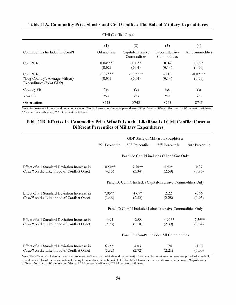
54

Table 11A. Commodity Price Shocks and Civil Conflict: The Role of Military Expenditures

Civil Conflict Onset

(1) (2) (3) (4)

Commodities Included in ComPI Oil and Gas

Capital-Intensive

Commodities

Labor Intensive

Commodities

All Commodities

ComPI, t-1 0.04***

(0.02)

0.03**

(0.01)

0.04

(0.14)

0.02*

(0.01)

ComPI, t-1

*Log Country's Average Military

Expenditures (% of GDP)

-0.02***

(0.01)

-0.02***

(0.01)

-0.19

(0.14)

-0.02***

(0.01)

Country FE Yes Yes Yes Yes

Year FE Yes Yes Yes Yes

Observations 8745 8745 8745 8745

Note: Estimates are from a conditional logit model. Standard errors are shown in parentheses. *Significantly different from zero at 90 percent confidence,

** 95 percent confidence, *** 99 percent confidence.

Table 11B. Effects of a Commodity Price Windfall on the Likelihood of Civil Conflict Onset at

Different Percentiles of Military Expenditures

GDP Share of Military Expenditures

25th Percentile 50th Percentile 75th Percentile 90th Percentile

Panel A: ComPI includes Oil and Gas Only

Effect of a 1 Standard Deviation Increase in

ComPI on the Likelihood of Conflict Onset

10.50**

(4.15)

7.50**

(3.34)

4.42*

(2.59)

0.37

(1.96)

Panel B: ComPI Includes Capital-Intensive Commodities Only

Effect of a 1 Standard Deviation Increase in

ComPI on the Likelihood of Conflict Onset

7.05**

(3.46)

4.67*

(2.82)

2.22

(2.28)

-0.99

(1.93)

Panel C: ComPI Includes Labor-Intensive Commodities Only

Effect of a 1 Standard Deviation Increase in

ComPI on the Likelihood of Conflict Onset

-0.91

(2.78)

-2.88

(2.18)

-4.90**

(2.39)

-7.56**

(3.64)

Panel D: ComPI Includes All Commodities

Effect of a 1 Standard Deviation Increase in

ComPI on the Likelihood of Conflict Onset

6.25*

(3.32)

4.03

(2.72)

1.74

(2.21)

-1.27

(1.90)

Note: The effects of a 1 standard deviation increase in ComPI on the likelihood (in percent) of civil conflict onset are computed using the Delta method.

The effects are based on the estimates of the logit model shown in column (1) of Table 12A. Standard errors are shown in parentheses. *Significantly different from zero at 90 percent confidence, ** 95 percent confidence, *** 99 percent confidence.

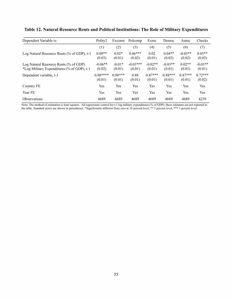
55

Table 12. Natural Resource Rents and Political Institutions: The Role of Military Expenditures

Dependent Variable is: Polity2 Exconst Polcomp Exrec Democ Autoc Checks

(1) (2) (3) (4) (5) (6) (7)

Log Natural Resource Rents (% of GDP), t-1 0.09**

(0.03)

0.02*

(0.01)

0.06***

(0.02)

0.02

(0.01)

0.04**

(0.02)

-0.05**

(0.02)

0.05**

(0.02)

Log Natural Resource Rents (% of GDP)

*Log Military Expenditures (% of GDP), t-1

-0.06**

(0.02)

-0.01*

(0.01)

-0.03***

(0.01)

-0.02**

(0.01)

-0.03**

(0.01)

0.02**

(0.01)

-0.03**

(0.01)

Dependent variable, t-1 0.88****

(0.01)

0.88***

(0.01)

0.88

(0.01)

0.87***

(0.01)

0.88***

(0.01)

0.87***

(0.01)

0.72***

(0.02)

Country FE Yes Yes Yes Yes Yes Yes Yes

Year FE Yes Yes Yes Yes Yes Yes Yes

Observations 4689 4689 4689 4689 4689 4689 4239

Note: The method of estimation is least squares. All regressions control for t-1 log military expenditures (% of GDP); these estimates are not reported in

the table. Standard errors are shown in parentheses. *Significantly different from zero at 10 percent level, ** 5 percent level, *** 1 percent level.

56

Table 13. Natural Resource Rents and Economic Growth: The Role of Military Expenditures

Dependent Variable is: PPP GDP

per capita

Growth (in %

per annum)

Log Domestic

Investment

(% of GDP)

Log Domestic

Saving

(% of GDP)

Government

Consumption

(% of GDP)

(1) (2) (3) (4)

Log Natural Resource Rents (% of GDP), t-1 0.96***

(0.33)

0.04**

(0.36)

0.10***

(0.03)

-0.34*

(0.18)

Log Natural Resource Rents (% of GDP) *Log

Military Expenditures (% of GDP), t-1

-0.70***

(0.26)

-0.02**

(0.01)

-0.03*

(0.02)

0.33**

(0.17)

Country FE Yes Yes Yes Yes

Year FE Yes Yes Yes Yes

Observations 3149 4269 4269 4662

Note: The method of estimation is least squares. All regressions control for t-1 log military expenditures (% of GDP) and in addition, in column (1), log GDP per capita in t-1; these estimates are not reported in the table. Huber robust standard errors (shown in parentheses) are clustered at the

country level. *Significantly different from zero at 10 percent level, ** 5 percent level, *** 1 percent level.

57

Table 14. Natural Resource Rents and Economic Growth: The Role of Military Expenditures

(Robustness: 5-Year Panel Data)

Dependent Variable is: PPP GDP

per capita

Growth (in %

per annum)

Log Domestic

Investment

(% of GDP)

Log Domestic

Saving

(% of GDP)

Government

Consumption

(% of GDP)

(1) (2) (3) (4)

Log Natural Resource Rents

(% of GDP), t-1

0.77**

(0.32)

0.06**

(0.02)

0.12**

(0.04)

-0.21

(0.22)

Log Natural Resource Rents (% of GDP) *Log

Military Expenditures (% of GDP), t-1

-0.49***

(0.18)

-0.03**

(0.01)

-0.04*

(0.02)

0.51***

(0.18)

Country FE Yes Yes Yes Yes

Year FE Yes Yes Yes Yes

Observations 643 888 888 977

Note: The method of estimation is least squares. All regressions control for t-1 log military expenditures (% of GDP) and in addition, in column (1), log

GDP per capita in t-1; these estimates are not reported in the table. Huber robust standard errors (shown in parentheses) are clustered at the country level. *Significantly different from zero at 10 percent level, ** 5 percent level, *** 1 percent level.

58

Table 15. Natural Resource Rents and Schooling: The Role of Military Expenditures

Dependent Variable is: Government

Expenditure on

Education

(% of Total

Government

Expenditures)

School Enrolment

(Secondary and

Primary)

School Enrolment

(Secondary)

School Enrolment

(Primary)

(1) (2) (3) (4)

Log Natural Resource Rents

(% of GDP), t-1

0.90**

(0.42)

2.31***

(0.79)

3.37***

(1.04)

2.16***

(0.71)

Log Natural Resource Rents (% of GDP) *Log

Military Expenditures (% of GDP), t-1

-0.59**

(0.27)

-0.74**

(0.35)

-1.40***

(0.52)

-0.67**

(0.32)

Country FE Yes Yes Yes Yes

Year FE Yes Yes Yes Yes

Observations 530 830 842 921

Note: The method of estimation is least squares. All regressions control for t-1 log military expenditures (% of GDP); these estimates are not reported in the table. Huber robust standard errors (shown in parentheses) are clustered at the country level. *Significantly different from zero at 10 percent level, ** 5

percent level, *** 1 percent level.

59

Table 16. Natural Resource Rents and Poverty: The Role of Military Expenditures

Dependent Variable is: Poverty

Rate

$1.9 a Day

Poverty

Rate

$3.2 a Day

Poverty

Rate

$5.5 a Day

Poverty

Gap

$1.9 a Day

Poverty

Gap

$3.2 a Day

Poverty

Gap

$5.5 a Day

(1) (2) (3) (4) (5) (6)

Log Natural Resource Rents

(% of GDP), t-1

-2.59**

(1.01)

-3.33**

(1.32)

-3.15**

(1.52)

-0.85*

(0.50)

-1.76**

(0.74)

-2.33**

(0.97)

Log Natural Resource Rents (% of

GDP) *Log Military Expenditures

(% of GDP), t-1

1.37**

(0.60)

1.70**

(0.81)

1.16

(0.95)

0.39

(0.29)

0.89**

(0.44)

1.10*

(0.59)

Country FE Yes Yes Yes Yes Yes Yes

Year FE Yes Yes Yes Yes Yes Yes

Observations 339 339 339 339 339 339

Note: The method of estimation is least squares. All regressions control for t-1 log military expenditures (% of GDP) and the poverty rate in t-1; these

estimates are not reported in the table. Huber robust standard errors (shown in parentheses) are clustered at the country level. *Significantly different from zero at 10 percent level, ** 5 percent level, *** 1 percent level.

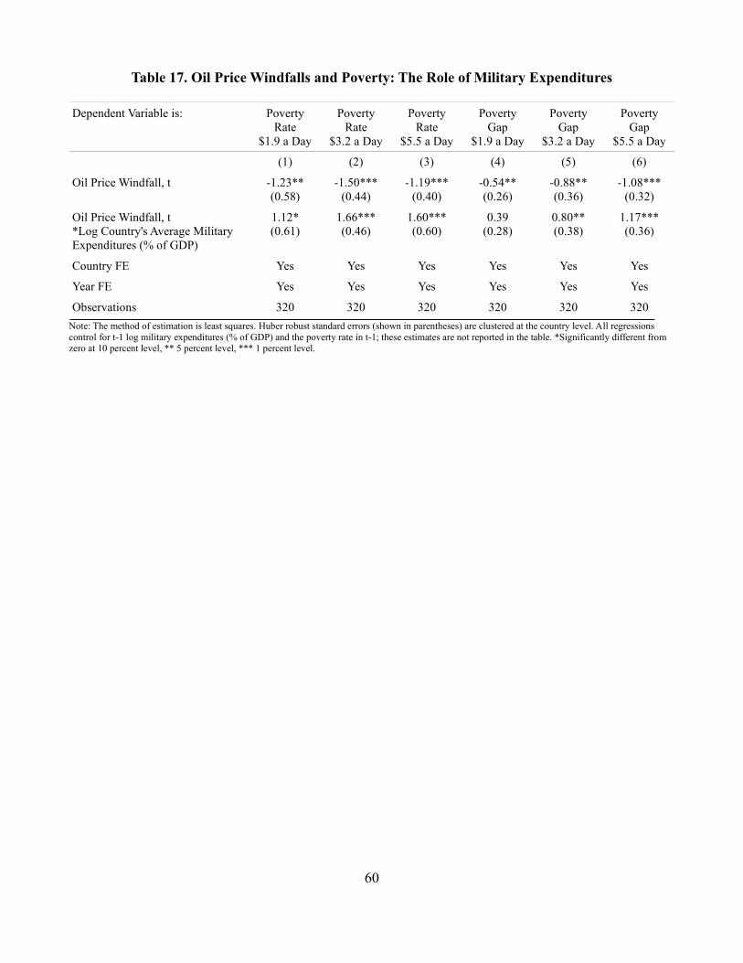
60

Table 17. Oil Price Windfalls and Poverty: The Role of Military Expenditures

Dependent Variable is: Poverty

Rate

$1.9 a Day

Poverty

Rate

$3.2 a Day

Poverty

Rate

$5.5 a Day

Poverty

Gap

$1.9 a Day

Poverty

Gap

$3.2 a Day

Poverty

Gap

$5.5 a Day

(1) (2) (3) (4) (5) (6)

Oil Price Windfall, t -1.23**

(0.58)

-1.50***

(0.44)

-1.19***

(0.40)

-0.54**

(0.26)

-0.88**

(0.36)

-1.08***

(0.32)

Oil Price Windfall, t

*Log Country's Average Military

Expenditures (% of GDP)

1.12*

(0.61)

1.66***

(0.46)

1.60***

(0.60)

0.39

(0.28)

0.80**

(0.38)

1.17***

(0.36)

Country FE Yes Yes Yes Yes Yes Yes

Year FE Yes Yes Yes Yes Yes Yes

Observations 320 320 320 320 320 320

Note: The method of estimation is least squares. Huber robust standard errors (shown in parentheses) are clustered at the country level. All regressions

control for t-1 log military expenditures (% of GDP) and the poverty rate in t-1; these estimates are not reported in the table. *Significantly different from zero at 10 percent level, ** 5 percent level, *** 1 percent level.

61

Appendix Table 1. Summary Statistics

Mean Stdv. Data Source

Total Natural Resource Rents, in billion USD 848 4010 WDI

Log Total Natural Resource Rents 24.5 2.69 WDI

Total Natural Resource Rents as a % of GDP 7.59 11.35 WDI

Log Total Natural Resource Rents as a % of GDP 0.47 2.44 WDI

Military Expenditures as a % of GDP 2.91 3.76 WDI

Log Military Expenditure as % of GDP 0.65 2.93 WDI

Military Expenditures as a % of Central Gov. Expenditures 10.67 9.18 WDI

Log Military Expenditures as a % of Central Gov. Expenditures 2.05 0.82 WDI

Civil Conflict Onset 0.05 0.22 PRIO

Civil War Onset 0.03 0.16 COW

Civil War Onset 0.02 0.12 Collier and Hoeffler

Civil War Onset 0.02 0.14 Fearon and Laitin

Civil War Onset 0.02 0.15 Sambanis

Revised Combined Polity Score (Polity2) 2.73 7.16 Polity IV

Executive Constraints Score (Exconst) 4.70 2.29 Polity IV

Political Competition Score (Polcomp) 6.33 3.48 Polity IV

Executive Recruitment Score (Exrec) 6.13 2.30 Polity IV

Democracy Score (Democ) 5.23 4.09 Polity IV

Autocracy Score (Autoc) 2.50 3.28 Polity IV

Checks and Balances Score (Checks) 2.72 1.76 DPI

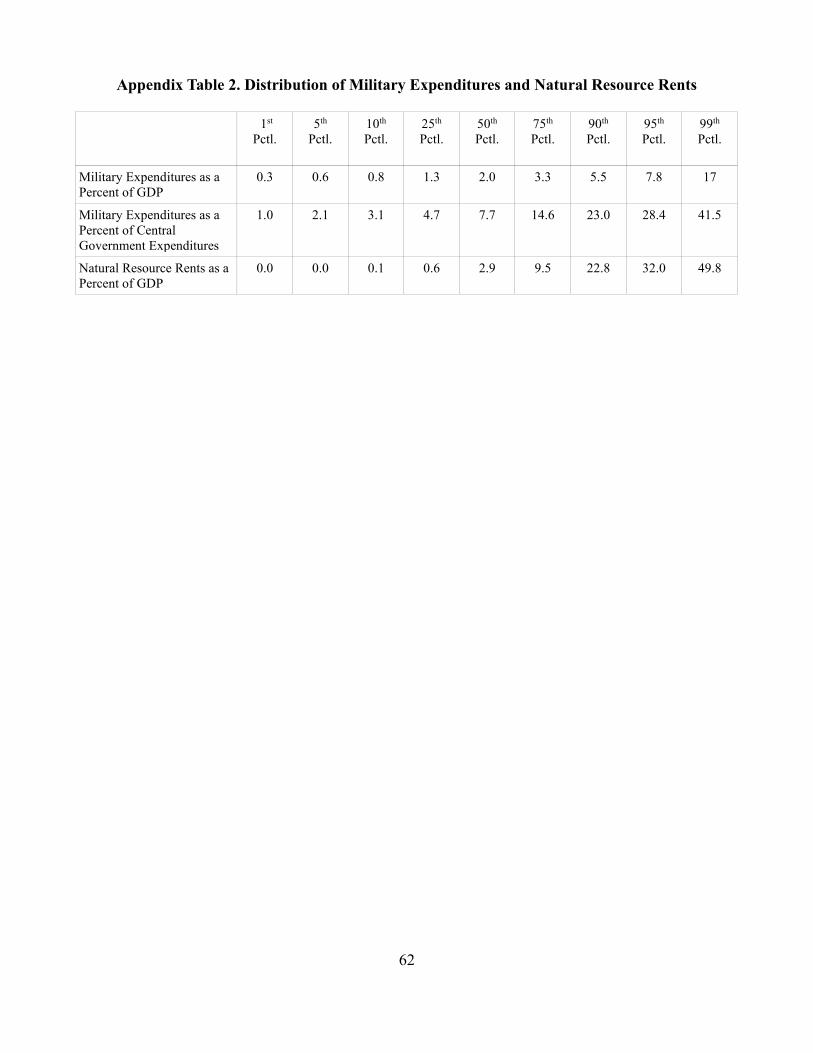
62

Appendix Table 2. Distribution of Military Expenditures and Natural Resource Rents

1st

Pctl.

5th

Pctl.

10th

Pctl.

25th

Pctl.

50th

Pctl.

75th

Pctl.

90th

Pctl.

95th

Pctl.

99th

Pctl.

Military Expenditures as a

Percent of GDP

0.3 0.6 0.8 1.3 2.0 3.3 5.5 7.8 17

Military Expenditures as a

Percent of Central

Government Expenditures

1.0 2.1 3.1 4.7 7.7 14.6 23.0 28.4 41.5

Natural Resource Rents as a

Percent of GDP

0.0 0.0 0.1 0.6 2.9 9.5 22.8 32.0 49.8

63

Appendix Table 3. Sample Split

Civil Conflict Onset

(1) (2) (3) (4)

Panel A: Low and Intermediate Military Expenditures % of GDP

Log Natural Resource

Rents (% of GDP), t

0.16***

(0.05)

0.17***

(0.05)

0.14

(0.12)

0.26*

(0.14)

Country FE No No Yes Yes

Year FE No Yes No Yes

Observations 4191 4191 4191 4191

Panel B: High Military Expenditures % of GDP

Log Natural Resource

Rents (% of GDP), t

-0.06*

(0.03)

-0.08**

(0.04)

0.01

(0.09)

-0.05

(0.12)

Country FE No No Yes Yes

Year FE No Yes No Yes

Observations 1374 1374 1374 1374

Note: Estimates in columns (1) and (2) are from a logit model; in columns (3) and (4) conditional logit model. Panel A reports estimates for the sub-sample

with low and intermediate military expenditures as a share of GDP (75th percentile and below). Panel B reports estimates for the sub-sample with high

military expenditures (above 75th percentile). Standard errors are shown in parentheses. *Significantly different from zero at 10 percent level, ** 5 percent level, *** 1 percent level.

64

Appendix Table 4. Ciccone (2019)

“International Commodity Prices and Civil War Outbreak: New Evidence for Sub-Saharan Africa and

Beyond”

(1) (2) (3) (4) (5) (6)

Replication

Appendix

Table 8,

column 3

Data on

Military

Expenditures

Not Missing

Military

Expenditures

% of GDP

Smaller Than

2 Percent

Military

Expenditures

% of GDP

Smaller Than

2 Percent

Military

Expenditures

% of GDP

Larger Than 2

Percent

Military

Expenditures

% of GDP

Larger Than 2

Percent

Price Shock, t -0.021**

(0.011)

-0.030*

(0.017)

-0.013

(0.014)

0.007

(0.014)

-0.038

(0.036)

-0.028

(0.033)

Price Shock, t-1 -0.022

(0.014)

-0.059**

(0.023)

-0.017

(0.021)

0.007

(0.016)

-0.074*

(0.042)

-0.071*

(0.042)

Price Shock, t-2 -0.017

(0.012)

-0.043**

(0.022)

0.012*

(0.007)

0.026**

(0.012)

-0.073*

(0.039)

-0.056

(0.040)

Country FE Yes Yes Yes Yes Yes Yes

Country Trend Yes Yes Yes Yes Yes Yes

Year FE Yes Yes Yes No Yes No

Observations 5019 3066 1574 1574 1492 1492

65

Appendix Table 5. Berman, Couttenier, Rohner, and Thoenig (2017, AER)

“This Mine is Mine: How Minerals Fuel Conflicts in Africa”

(1) (2) (3) (4) (5) (6)

Replication of

Col 1 Table 2

of Berman et

al. (2017)

Replication of

Col 1 Table 2

of Berman et

al. (2017)

for Military

Expenditures

Data

not Missing

Military

Expenditures

Less Than 8.7

% of Central

Government

Expenditures

(Bottom 25th

Percentile)

Military

Expenditures

Less Than 11

% of Central

Government

Expenditures

(Bottom 50th

Percentile)

Military

Expenditures

More Than 11

% of Central

Government

Expenditures

(Top 50th

Percentile)

Military

Expenditures

More Than 15

% of Central

Government

Expenditures

(Top 75th

Percentile)

ln price mines > 0 0.086**

(0.034)

0.066**

(0.034)

0.138**

(0.056)

0.079**

(0.037)

-0.008

(0.061)

-0.449

(0.503)

Country-Year FE Yes Yes Yes Yes Yes Yes

Cell FE Yes Yes Yes Yes Yes Yes

Observations 143768 65143 16267 32641 32502 16730

Note: Standard errors are shown in parentheses. Column (1) replicates column (1) of Table 2 in Berman et al. (2017). Only

the estimate of α3 on ln price mines > 0 is reported (refer to Berman et al., 2017, equation (1), on page 1573); the estimates

on the other variables are not reported. Column (2) shows estimates for the sample with available data on military

expenditures as percent of central government expenditures. Estimates for countries with low military expenditures are

shown in columns (3) and (4). Specifically, column (3) shows estimates for countries where military expenditures are less

than 8.7 % of central government expenditures (the bottom 25th percentile in the sample distribution of military

expenditures as a percent of central government expenditures); column (4) shows estimates for countries where military

expenditures are less than 11 % of central government expenditures (the bottom 50th percentile in the sample distribution of

military expenditures as a percent of central government expenditures). Estimates for countries with high military

expenditures are shown in columns (5) and (6). Specifically, column (5) shows estimates for countries where military

expenditures exceed 11 % of central government expenditures (the top 50th percentile in the sample distribution of military

expenditures as a percent of central government expenditures); column (6) shows estimates for countries where military

expenditures exceed 11 % of central government expenditures (the top 25th percentile in the sample distribution of military

expenditures as a percent of central government expenditures).

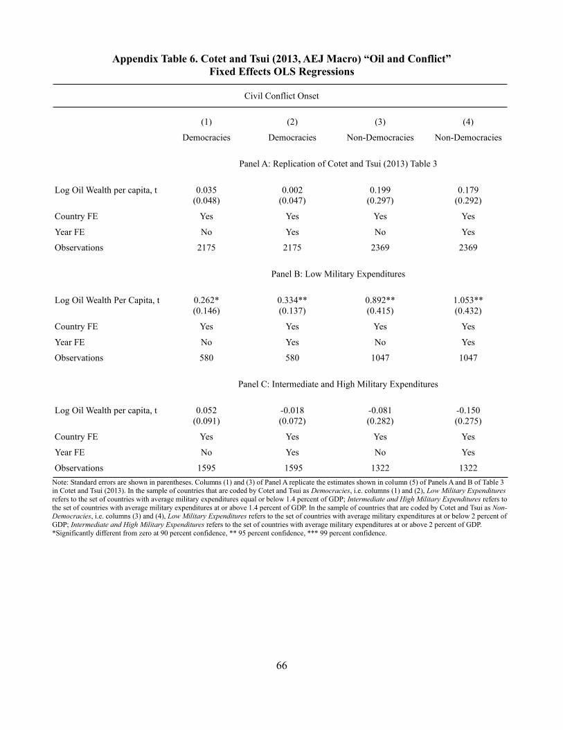
66

Appendix Table 6. Cotet and Tsui (2013, AEJ Macro) “Oil and Conflict”

Fixed Effects OLS Regressions

Civil Conflict Onset

(1) (2) (3) (4)

Democracies Democracies Non-Democracies Non-Democracies

Panel A: Replication of Cotet and Tsui (2013) Table 3

Log Oil Wealth per capita, t 0.035

(0.048)

0.002

(0.047)

0.199

(0.297)

0.179

(0.292)

Country FE Yes Yes Yes Yes

Year FE No Yes No Yes

Observations 2175 2175 2369 2369

Panel B: Low Military Expenditures

Log Oil Wealth Per Capita, t 0.262*

(0.146)

0.334**

(0.137)

0.892**

(0.415)

1.053**

(0.432)

Country FE Yes Yes Yes Yes

Year FE No Yes No Yes

Observations 580 580 1047 1047

Panel C: Intermediate and High Military Expenditures

Log Oil Wealth per capita, t 0.052

(0.091)

-0.018

(0.072)

-0.081

(0.282)

-0.150

(0.275)

Country FE Yes Yes Yes Yes

Year FE No Yes No Yes

Observations 1595 1595 1322 1322

Note: Standard errors are shown in parentheses. Columns (1) and (3) of Panel A replicate the estimates shown in column (5) of Panels A and B of Table 3 in Cotet and Tsui (2013). In the sample of countries that are coded by Cotet and Tsui as Democracies, i.e. columns (1) and (2), Low Military Expenditures

refers to the set of countries with average military expenditures equal or below 1.4 percent of GDP; Intermediate and High Military Expenditures refers to

the set of countries with average military expenditures at or above 1.4 percent of GDP. In the sample of countries that are coded by Cotet and Tsui as Non-Democracies, i.e. columns (3) and (4), Low Military Expenditures refers to the set of countries with average military expenditures at or below 2 percent of

GDP; Intermediate and High Military Expenditures refers to the set of countries with average military expenditures at or above 2 percent of GDP.

*Significantly different from zero at 90 percent confidence, ** 95 percent confidence, *** 99 percent confidence.

67

Appendix Table 7. Cotet and Tsui (2013, AEJ Macro) “Oil and Conflict”

Fixed Effects 2SLS Regressions

Civil Conflict Onset

(1) (2) (3) (4)

Democracies Democracies Non-Democracies Non-Democracies

Panel A: Low Military Expenditures

Log Oil Wealth Per Capita, t 0.263*

(0.137)

0.333***

(0.120)

0.996***

(0.378)

1.157***

(0.394)

Kleibergen Paap F-Stat 2.6*105 2.3*104 2000 2132

Country FE Yes Yes Yes Yes

Year FE No Yes No Yes

Observations 580 580 1047 1047

Panel B: Intermediate and High Military Expenditures

Log Oil Wealth Per Capita, t 0.030

(0.086)

-0.027

(0.070)

-0.060

(0.292)

-0.128

(0.271)

Kleibergen Paap F-Stat 2.8*104 2.8*104 1070 4116

Country FE Yes Yes Yes Yes

Year FE No Yes No Yes

Observations 1595 1595 1322 1322

Panel C: Replication of Cotet and Tsui (2013) Table 3

Log Oil Wealth Per Capita, t 0.019

(0.047)

-0.004

(0.047)

0.241

(0.304)

0.215

(0.292)

Kleibergen Paap F-Stat 9.3*104 2.6*104 1794 4225

Country FE Yes Yes Yes Yes

Year FE No No Yes Yes

Observations 2175 2175 2369 2369

Note: Standard errors are shown in parentheses. Columns (1) and (3) of Panel C replicate the two-stage least squares estimates shown in column (6) of

Panels A and B of Table 3 in Cotet and Tsui (2013). In all columns, the instrument set is the same as in Cotet and Tsui (2013): log (out-of-region natural

disaster), log (oil reserves per capita), and their product.In the sample of countries that are coded by Cotet and Tsui as Democracies, i.e. columns (1) and

(2), Low Military Expenditures refers to the set of countries with average military expenditures equal or below 1.4 percent of GDP; High Military Expenditures refers to the set of countries with average military expenditures at or above 1.4 percent of GDP. In the sample of countries that are coded by

Cotet and Tsui as Non-Democracies, i.e. columns (3) and (4), Low Military Expenditures refers to the set of countries with average military expenditures at

or below 2 percent of GDP; High Military Expenditures refers to the set of countries with average military expenditures at or above 2 percent of GDP. *Significantly different from zero at 90 percent confidence, ** 95 percent confidence, *** 99 percent confidence.

68

Appendix Table 8. Military Influence on Government and Military Expenditure Shares

Share of Military Expenditures in GDP

Share of Military Expenditures in Central

Government Expenditures

(1) (2) (3) (4) (5) (6)

Chief Executive is a

Military Officer

0.80**

(0.36)

7.97***

(2.79)

Defense Minister is a

Military Officer

0.66**

(0.28)

4.73***

(1.66)

Military Dictatorship 0.31*

(0.18)

5.39***

(1.66)

Country Fixed Effects Yes Yes Yes Yes Yes Yes

Observations 4090 4039 4549 2265 2260 1974 Note: The dependent variable in columns (1)-(3) is the share of military expenditures in GDP (in percent); columns (4)-(6) the share of military expenditures in central government expenditures (in percent). The method of estimation is least squares. Huber robust standard errors (shown in

parentheses) are clustered at the country level. *Significantly different from zero at 10 percent level, ** 5 percent level, *** 1 percent level.

69

Appendix Table 9. Oil Price Windfalls and Civil Conflict Onset

Civil Conflict Onset

(1) (2) (3)

Panel A: Strong Military Influence on Government

Chief Executive is a

Military Officer

Defense Minister is a

Military Officer

Military Dictatorship

Oil Price Windfall -0.13

(0.15)

0.04

(0.10)

-0.11

(0.12)

Country Fixed Effects Yes Yes Yes

Time Fixed Effects Yes Yes Yes

Observations 559 813 771

Panel B: Weak Military Influence on Government

Chief Executive is not a

Military Officer

Defense Minister is not a

Military Officer

No Military Dictatorship

Oil Price Windfall 0.17**

(0.07)

0.31**

(0.15)

0.05*

(0.03)

Country Fixed Effects Yes Yes Yes

Time Fixed Effects Yes Yes Yes

Observations 1788 1469 2491 Note: The dependent variable is civil conflict onset. Panel A report estimates for the subset of countries with strong military influence on government;

Panel B weak military influence on government. The estimates are from a conditional logit model. Standard errors are shown in parentheses. *Significantly

different from zero at 10 percent level, ** 5 percent level, *** 1 percent level.