This paper presents preliminary findings and is being distributed to economists and other interested readers solely to stimulate discussion and elicit comments. The views expressed in this paper are those of the authors and do not necessarily reflect the position of the Federal Reserve Bank of New York or the Federal Reserve System. Any errors or omissions are the responsibility of the authors. Federal Reserve Bank of New York Staff Reports The Impact of Supervision on Bank Performance Beverly Hirtle Anna Kovner Matthew Plosser Staff Report No. 768 March 2016 Revised May 2019
Transcript
This paper presents preliminary findings and is being distributed to economists and other interested readers solely to stimulate discussion and elicit comments. The views expressed in this paper are those of the authors and do not necessarily reflect the position of the Federal Reserve Bank of New York or the Federal Reserve System. Any errors or omissions are the responsibility of the authors.
Federal Reserve Bank of New York Staff Reports
The Impact of Supervision on Bank Performance
Beverly Hirtle Anna Kovner
Matthew Plosser
Staff Report No. 768 March 2016
Revised May 2019
The Impact of Supervision on Bank Performance Beverly Hirtle, Anna Kovner, and Matthew Plosser Federal Reserve Bank of New York Staff Reports, no. 768 March 2016; revised May 2019 JEL classification: G21, G28
Abstract
We explore the impact of supervision on the riskiness, profitability, and growth of U.S. banks. Using data on supervisors’ time use, we demonstrate that the top-ranked banks by size within a supervisory district receive more attention from supervisors, even after controlling for size, complexity, risk, and other characteristics. Using a matched sample approach, we find that these top-ranked banks that receive more supervisory attention hold less risky loan portfolios, are less volatile, and are less sensitive to industry downturns, but do not have slower growth or profitability. Our results underscore the distinct role of supervision in mitigating banking sector risk.
Key words: bank supervision, bank regulation, bank performance
_________________
Hirtle, Kovner, Plosser: Federal Reserve Bank of New York (emails: [email protected], [email protected], [email protected]). The authors thank Maya Bidanda, Angela Deng, Brandon Zborowski, and Samantha Zeller for excellent research assistance. They thank Mark Carey, Stefan Lewellen, Mark Levonian, Antoinette Schoar, Philip Strahan, Vish Viswanathan, two anonymous referees, and seminar participants at the Federal Reserve Bank of New York, the AFA Annual Meetings, the Bank of France, the NBER Summer Institute, and the FDIC/JFSR Bank Research Conference. The views expressed in this paper are those of the authors and do not necessarily reflect the position of the Federal Reserve Bank of New York or the Federal Reserve System.
To view the authors’ disclosure statements, visit https://www.newyorkfed.org/research/ author_disclosure/ad_sr768.
Supervision and regulation are critical tools for the promotion of stability and soundness
in the financial sector. Despite supervision’s key role, it is rarely examined separately from
regulation and relatively little is known about the distinct impact of supervisory efforts. This
paper exploits new supervisory data and develops a novel identification strategy to estimate
the impact of greater supervision on bank risk-taking and performance. We find that more
supervision adds value over and above the effects of regulation. Banks that receive more
supervisory attention have less risky loan portfolios, are less volatile and less sensitive to
industry downturns, but do not have lower growth or profitability.
While prior work has examined specific supervisory actions such as examinations or
enforcement actions, little is known about the effectiveness of supervisors’ more general
efforts to promote sound risk management. For example, supervisors meet frequently with
bank management, discussing both specific issues regarding activities at the firm and more
general perspectives on the industry environment and outlook. These conversations, along
with analysis of internal firm reports and external data, allow supervisors to understand
bank risks and procedures and to put these in context relative to the industry. By focusing
on a broad concept of supervisory attention, our analysis captures the breadth of supervisory
efforts without restriction to a single supervisory program.
Reflecting the potential externalities of bank failures, supervisors seek to reduce failure
risk relative to what banks themselves might otherwise choose. Our analysis is designed
to evaluate whether supervisors achieve their objectives and at what cost to financial in-
termediation. Actual bank failures are infrequent, especially among the largest firms that
receive the most supervisory attention, therefore we rely on a range of risk metrics covering
lending activities (e.g., loan losses and reserving practices) as well as firm-wide metrics such
as overall earnings volatility and market measures of riskiness.
The key empirical hurdle to identifying the impact of supervision is that larger and riskier
firms receive more supervisory attention. We surmount this by exploiting the structure of
supervisory responsibilities within the Federal Reserve System, under which bank holding
1
companies (BHCs or “banks”) are geographically assigned to one of twelve Federal Reserve
Districts. We hypothesize that within each district, the largest institutions receive more
supervisory attention, ceteris paribus, than institutions that are not among the largest.
Although supervisory hours do not capture all aspects of supervisory intensity, we validate
this hypothesis with proprietary Federal Reserve data, showing that examiners spend more
time at the largest firms in a district, even when controlling for firm characteristics like size,
market share, complexity, and supervisory rating.
We match top-ranked bank holding companies in Federal Reserve districts by size, deposit
market share, organizational complexity, types of banking subsidiaries, diversity of lending
activities and other characteristics to similar banks in other districts that are not among
the largest. Doing so allows us to construct a sample of banks that are observably similar
but with varying ranks in their Federal Reserve districts. Our focus is on controlling for
differences across banks that might be correlated with rank and performance, but to avoid
matching on outcome variables that might be directly influenced by supervision. We thus
compare outcomes for banks that are among the largest in a district to otherwise similar
banks that are not among the largest in other districts, and interpret differences in outcomes
as reflecting the impact of greater supervisory attention.
Our findings suggest that enhanced supervisory attention is associated with lower risk.
Banks among the largest in a district have accounting earnings and market returns that are
less volatile than otherwise similar BHCs. Top-ranked banks on average have non-performing
loan ratios that are roughly 15-25% lower than peers that are not among the top in their
district. These firms also appear to engage in more conservative loan loss reserving practices.
The reduction in risk is greater during downturns, precisely when the externalities of failure
are costlier. With respect to volatility, our findings suggest that a 20% increase in supervisory
hours is associated with a 9-10% decrease in risk as measured by the volatility of earnings,
a reduction in distance to default equivalent to 150-200 bps of additional capital.
Importantly, while top-ranked BHCs appear less risky, they do not have lower profitability
2
nor do they exhibit significantly slower loan or asset growth. There are no meaningful
differences in market or accounting measures of profitability, including return on assets and
excess stock price returns, between the top-ranked BHCs and their matches. Further, the
market Sharpe ratio of top-ranked BHCs is similar to that of BHCs not among the top
size-ranked firms. These findings are consistent with the notion that additional supervisory
attention is associated with lower risk exposure but has a positive-to-neutral impact on the
risk-adjusted performance of BHCs. Our results suggest that there are meaningful social
welfare benefits to supervision in the form of decreased risk of failure of large banks without
significant reduction in their intermediation activities.
Our identifying assumption is that being among the largest firms in a Federal Reserve
District is not associated with other unobserved factors that also impact bank performance.
We take a number of steps to account for other possibilities. For example, one critical
difference might be related to differences in risk across districts. To better account for
district-level differences, we consider an empirical specification that uses a larger matched
sample and controls for district-quarter fixed effects to account for unobserved differences
across districts and over time. Another difference could be in competitiveness and franchise
value. We consider additional matching criteria, including recent firm performance and
proxies for franchise value such as market-to-book. Our conclusions are robust to these
various alternative specifications.
Our results suggest that increased supervisory attention results in lower risk without sig-
nificantly reduced performance. Nevertheless, our empirical approach does not shed light on
the specific actions by which supervision achieves these outcomes. One plausible mechanism
is that supervision helps to resolve principal-agent problems within the firm. In particular,
enhanced supervision may result in more weight being given inside the firm to concerns of
risk managers, resulting in more disciplined risk-taking. In this way, supervisors may also
improve a bank’s risk culture, by fostering increased attention to risk as a balance to a focus
on short-term profitability. Supervisory requests for risk and activity information may cause
3
banks to invest in data and technology systems that then enable them to manage their busi-
ness more efficiently over the long run. Finally, because supervisors oversee many banks,
they may transmit knowledge of best practices in the industry when they set expectations
and provide feedback to banks about their risk management practices.
Much of the previous work on the supervision and regulation of banks focuses on the
impact of regulation, though the distinction between supervision and regulation is not al-
ways clearly recognized or articulated.1 Fewer papers focus specifically on supervision dis-
tinctly defined. Some of these papers examine the information content of supervisory ratings
(Cargill, 1989; Cole and Gunther, 1995; Hirtle and Lopez, 1999; Berger, Davies, and Flan-
nery, 2000) and examinations (Berger and Davies, 1998) but not specifically the impact of
supervision on bank outcomes. Several papers have examined whether supervisory standards
how tough examiners are in assessing risk at banks affect loan origination and loan growth
(Peek and Rosengren, 1995; Swindle, 1995; Krainer and Lopez, 2009; Kiser, Prager, and
Scott, 2012; Bassett, Lee, and Spiller, 2012; Bassett and Marsh, 2014) with most finding
that tougher supervisory standards are associated with slower loan growth and/or higher
origination standards. Others have examined the use of enforcement actions on bank sector
risk (e.g. Delis and Staikouras, 2011). Relative to the extant literature, our use of supervi-
sory attention allows us to estimate supervision’s impact in a way that considers the breadth
of supervisory interactions with firms.
A second contribution of our paper is that we develop a new identification strategy based
on the structure of supervision at the Federal Reserve. Plausibly exogenous variation in su-
pervisory attention allows us to go beyond correlations to discern the impact of supervision.
The paper is similar in this spirit to recent work that examines state versus federal banking
supervisors including Agarwal, Lucca, Seru, and Trebbi (2014), which finds persistent dif-
1For instance, there is a substantial body of work examining the impact of regulatory capital requirements(for a recent example, see Bridges, Gregory, Nielsen, Pezzini, Radia, and Spaltro, 2014) and of legislativechanges that enabled previously prohibited cross-state bank mergers or mergers involving commercial banksand non-banking financial companies (see, for instance, Morgan, Bertrand, and Strahan, 2004; Jayaratneand Strahan, 1996).
4
ferences between state and federal banking supervisors in the rating of commercial banks,
and Rezende (2011), which finds that banks switching between national and state banking
charters typically receive an upgraded rating from their new supervisor. Most closely related,
Rezende and Wu (2014) employ a regression discontinuity approach to look at a sample of
U.S. banks and find that more frequent mandated examinations are associated with increased
profitability and lower loan losses. Recent work investigating the impact of supervisory of-
fice closures (Gopalan, Kalda, and Manela, 2017; Hagendorff, Lim, and Armitage, 2017)
suggests that a removal of nearby supervisors results in greater risk and lower profitability;
to the extent closures are a proxy for a reduction in supervisory attentiveness, these studies
corroborate our findings. In comparison to these papers, we focus on supervisory attention
more broadly rather than a specific activity like examinations; we demonstrate variation in
attention using novel data on the time supervisors spend at institutions; and, we are able to
consider the impact on relatively large firms.
While we consider several alternative explanations for our results, it is difficult to capture
constructs such as franchise value and market competition. To the extent our matching
criteria fails to capture these factors, we cannot rule out the possibility that these forces
could explain some of the reduction in risk that we attribute to supervisory attention. In
addition, we cannot rule out other sources of unobserved heterogeneity empirically. For
example, we do not observe the quality of supervision. While unlikely, if supervisory hours
are more productive in districts with smaller banks, then supervisory quality could explain
some of our findings.
The paper is organized as follows. Section I describes the role of prudential supervision
within the Federal Reserve and develops hypotheses related to supervisory attention and
bank outcomes. Section II outlines our identification strategy, describes the supervisory
hours data and presents analysis of differences in supervisory hours for the largest firms
in a district. Section III outlines our empirical methodology for assessing the impact of
supervision, including identifying a matched sample of BHCs. Section IV summarizes our
5
core empirical results and Section V considers alternative empirical specifications. Section VI
concludes.
I. Prudential supervision
The overarching objective of supervision is to identify and remediate conditions that
could threaten banks’ immediate health or long-term viability. Toward that end, pruden-
tial supervision encompasses a range of supervisory activities that support both traditional
efforts to ensure compliance with law and regulation as well as more modern, “prudential”
work to monitor for unsafe or unsound business practices. Federal Reserve supervisory ex-
pectations for certain activities, risk management or control procedures are often articulated
in Supervision and Regulation Letters (SR Letters) published by the Board of Governors
(Board of Governors of the Federal Reserve System, 2017c).
For many years, supervisors made their assessments based on a point-in-time analysis
of a bank, typically once per year, in the form of an annual examination. This process
was inherently backwards-looking because it focused on reviewing the quality of a bank’s
loans and other assets as of the exam date (Federal Deposit Insurance Corporation, 1997).
Beginning in the early 1990s, however, there was a transition toward a more holistic, forward-
looking approach to supervision, as supervisors sought to make institutions more robust in
the face of rapid financial innovation (Mishkin, 2001). For example, in 1995 the Federal
Reserve and the Office of the Comptroller of the Currency (OCC) formally announced that
they would be assessing banks’ risk management practices. Today a large share of the
interactions between bankers and supervisors, particularly for large banks, centers on risk
management, risk modeling and governance (Goldsmith-Pinkham, Hirtle, and Lucca, 2016).
Such forward-looking assessments of risk management and internal controls involve both
quantitative analysis and qualitative evaluations, often incorporating significant judgment.
These qualitative assessments are grounded in knowledge of industry standards and evolve
6
over time to adapt to financial innovation. Hence, modern supervisory activities rely on both
soft and hard information and are inherently difficult to quantify, both in terms of the work
that supervisors actually do and in terms of outcomes that focus on internal processes such
as risk management, controls and governance. Our empirical strategy is designed to capture
not only the impact of traditional, exam-based interactions but also the influence of these
more difficult to quantify interactions that are central to modern supervisory efforts.
If a supervisory assessment identifies shortcomings, supervisors possess a range of re-
sponses to require the firm to rectify the problems, from formal enforcement actions and
ratings downgrades, which can constrain bank activities, to more subtle warnings that work
via moral suasion. Supervisors assign confidential supervisory ratings (“1” indicates the low-
est level of supervisory concern, “5” indicates the highest) and issue supervisory actions that
direct the bank and its management and board to remediate unsafe or unsound practices or
conditions. Supervisory actions include matters requiring attention (MRAs), matters requir-
ing immediate attention (MRIAs), other informal enforcement actions such as memoranda
of understanding (MOUs), as well as written agreements, cease and desist orders, and fines.
MRAs and MRIAs are the most common supervisory actions. In general, informal actions,
such as MRAs and MRIAs are not publicly disclosed, while formal enforcement actions are
disclosed by the Federal Reserve Board.
Supervisory actions describe the specific supervisory concern in detail and generally re-
quire a time table for remediation. Banks subject to an action typically develop a remediation
plan, which is subject to approval by supervisors, who then track progress against the plan.
Failure to address the concerns raised by supervisors in a timely way can result in escalation
of the enforcement action from a confidential MRA or MRIA to a public enforcement action,
for instance or in restrictions on asset growth, dividends and share repurchases, or mergers
and acquisitions, as well as in fines (“civil money penalties”). Thus, supervisory actions can
have real consequences on the growth and business activities of a bank that fails to comply
7
with its supervisor’s directives.2
A. Hypotheses
Given externalities from bank failures, supervisors will prefer lower risk of failure or dis-
tress than bank managers, who do not internalize the costs of disruption of intermediation
services, including reduced credit supply and fire-sale-related asset price declines. If super-
visors are successful, banks that are subject to more intense supervision should take less
risk and use more conservative risk management practices. Greater supervisory focus on
risk management and governance could increase the influence of risk managers at the bank,
whose perspectives may be more aligned with supervisors than business area heads, help-
ing to solve an agency problem within the firm. Similarly, increased supervisory attention
could foster a stronger risk culture at banks by encouraging greater focus on risk exposure
as a counterbalance to incentives to generate short-run profits. Chaly, Hennessey, Menand,
Stiroh, and Tracy (2017) argue that supervisors’ impact on banks’ “cultural capital” is an
important channel for enhancing resiliency to foster stable provision of financial services.
Hence, one hypothesis is that greater supervisory efforts, all else equal, result in less risky
institutions.
Of course, there are many reasons that intense supervision might not result in safer banks.
Supervisors could fail to achieve their objectives due to resource constraints that could make
it difficult to work effectively at large and complex institutions, even with increased attention
to those firms. Also, a bank may have influence over its supervisors, resulting in greater
forbearance and, thus, more risk.
A second hypothesis is that increased supervisory attention results in less profitable,
slower growing banks. Compliance costs can lower profitability, and cross-country analysis
suggests supervision can reduce bank efficiency (e.g. Barth, Lin, Ma, Seade, and Song,
2Eisenbach, Haughwout, Hirtle, Kovner, Lucca, and Plosser (2017) contains a detailed description of therange of supervisory enforcement actions, the expectations on banks that are subject to such actions, andthe consequences of failing to comply.
8
2013). Supervisory concerns about risk management could result in banks’ having to make
investments in technology and data with large up-front costs, depressing near-term profits. In
addition, the empirical literature suggests that tougher supervisory standards are associated
with slower loan growth (e.g. Peek and Rosengren, 1995).
Alternatively, however, performance at more intensely supervised banks could be better
than at banks less closely supervised, especially on a risk-adjusted basis. For instance, invest-
ments in superior technology and information systems might enable business managers to
make better risk-return decisions or identify operational inefficiencies. Tarullo (2016) argues
that supervisory expectations from the Federal Reserve’s Comprehensive Capital Analysis
and Review (CCAR) program have resulted in large banks making significant improvements
to their information and risk management systems. Indeed, a senior risk manager argued
that consolidated risk management systems can allow banks to make better business deci-
sions by incorporating risk and return considerations in pricing, product development and
relationship management (Lam, 1999). Finally, since supervisors interact with a range of
firms, they might transmit best practices in risk management and controls via feedback to
firms about where they stand relative to supervisory expectations, fostering the spread of
best practice across the industry.
II. Identification Strategy
Our empirical analysis seeks to examine these two questions. First, is there evidence
that more intensive supervision is associated with lower risk? Second, do banks subject to
more intensive supervision grow more slowly, intermediate less credit or experience lower
profitability, either in absolute or risk-adjusted terms?
The primary empirical challenge in identifying the impact of supervision is that super-
visory attention is endogenously related to current and expected bank performance: super-
visors focus on poorly performing, risky BHCs. Supervisors also expend more resources on
9
large, complex institutions that pose a greater threat to financial stability.
In order to identify plausibly exogenous variation in supervisory attention, we exploit the
geographic assignment of BHCs to Federal Reserve districts. Within the Federal Reserve, the
Board of Governors has authority and responsibility for supervision of financial institutions,
and the supervisory activities of the Reserve Banks are conducted under delegated authority
from the Board. Under this delegated authority, day-to-day oversight of the firms is con-
ducted by the twelve regional Reserve Banks, which employ dedicated supervisory teams
responsible for the firms located in their respective districts. The location of the twelve
banks and the boundaries of the districts were determined pursuant to the Federal Reserve
Act of 1913 and reflect the various regions’ importance as banking centers in 1913 (Ghizoni,
2013).
Since that time, the district boundaries have remained the same despite significant
changes in the distribution of banks and the rise and fall of US banking centers. Conse-
quently, both the number and size of BHCs vary considerably across districts. Table I shows
the size of the largest BHCs in each of the 12 districts as of December 2014, along with
information about the median asset size of BHCs with assets above $500 million.3 The table
contains consolidated information on the highest level BHC in each firm’s corporate struc-
ture. The number of BHCs over $500 million ranges from a low of 57 in the Fourth District
(Cleveland) to a high of 157 in the Seventh (Chicago). The size of the largest BHCs in a
district also varies considerably, with the largest overall BHC in the Second District (New
York) at $2.6 trillion and the largest BHC in the Eighth District (St Louis) at $26 billion.
[Place Table I about here]
Each of the twelve Federal Reserve Banks supervises the bank holding companies head-
quartered in its geographic district, hosting dedicated supervisory teams responsible for these
3We report information on BHCs with assets greater than $500 million because these are the institutionsthat are required to submit FR Y-9C financial reports with the Federal Reserve. These reports, which containbalance sheet and income statement information, are a critical data source for our empirical analysis.
10
firms. The Reserve Banks have their own managerial hierarchy which makes hiring, perfor-
mance assessment and staff allocation decisions, subject to general oversight of its budget
and activities by the Board of Governors (Board of Governors of the Federal Reserve System,
2017a). These staffing decisions include the number of supervisory staff and their educa-
tional and professional backgrounds, as well as the way that supervisory staff are organized
to carry out their oversight objectives.
Some supervisory activities for BHCs are coordinated at the Federal Reserve System
level via committees composed of senior supervisors from the Reserve Banks and staff at
the Board of Governors. Starting in 2012, supervision of the very largest and most com-
plex bank holding companies has been coordinated across Reserve Banks and the Board
of Governors through the Large Institution Supervision Coordinating Committee (LISCC)
program (Board of Governors of the Federal Reserve System, 2017b). As described more
fully below, these firms drop out of our sample through the matching process. The nature of
our analysis is cross-district and typically excludes the largest BHCs; therefore, the impact
of system-wide programs is minimal to this study.
Given the district-level management of supervision, we posit that the largest BHCs in a
given district, all else equal, receive more supervisory attention. There are several reasons
why this might occur. Attention constraints on senior managers can require that they
prioritize a discrete set of the most important BHCs in their district (i.e. Miller’s Law4). This
hypothesis is motivated by research on the concept of span of control and the allocation of
managerial attention, such as Bolton and Dewatripont (1994), Garicano (2000), Geanakoplos
and Milgrom (1991), and Radner (1993). In this context, district leaders are subject to
cognitive costs, thus they focus attention on a discrete set of the largest firms (i.e. their
span of control) within their geographic area of responsibility.
Another possible rationale for this behavior is that supervisory teams in each district are
4Miller’s Law refers to the findings in a 1956 psychology paper “The Magical Number Seven, Plus orMinus Two: Some Limits on Our Capacity for Processing Information.” Miller (1956) describes variousexperiments on retaining sounds, colors, points, tastes, letters and numbers.
11
particularly concerned with large bank failures because they pose outsized negative external-
ities on the regional economy. As a result, supervisors could be allocated and incentivized
to spend time in a way that seeks to ensure the safety of the largest institutions under
the Reserve Bank’s purview. In practice, we cannot differentiate among these competing
motivations since they result in observationally equivalent outcomes.
Our analysis is ultimately indifferent as to which of these mechanisms results in greater
supervisory attention as long as the largest BHCs within a district receive additional at-
tention relative to similar BHCs for reasons unrelated to risk or performance each of the
rationales we outline above suggest that the largest banks in a district will receive additional
supervisory attention relative to otherwise similar firms.
A. Is Rank a Valid Proxy for Supervisory Attention?
We provide evidence in support of this hypothesis with a simple measure of supervisory
scrutiny: the hours spent by Federal Reserve supervisors examining a particular institution.
We use confidential Federal Reserve System managerial data on the time use of supervisors
at the Reserve Banks. Supervision personnel are required to self-report time-use. As part
of this reporting, they are instructed to indicate what hours of their time are spent directly
supervising a particular institution (as opposed to broadly contributing to the supervision of
a portfolio of banks or participating in other activities). The data include supervisory staff
in all twelve Federal Reserve districts over the period 2006 to 2014. We do not capture hours
that are not allocated to specific firms, or hours spent by Board of Governors supervisory
staff. To the extent that these hours substitute for supervisory hours by the Federal Reserve
Banks, their exclusion would serve to attenuate our results.
On a quarterly basis we aggregate the hours reported by examiners at each BHC and
its subsidiaries to generate a measure of supervisory attention for an organization the total
quantity of directly reported supervisory hours. Many BHC-quarters do not have directly
reported hours. If the institution has never received directly reported hours, then hours are
12
left as missing, reflecting the fact that the firm was supervised by a team that oversees a
portfolio of firms so supervisors did not directly record time use at individual institutions.
However, if a BHC has had reported hours in a prior quarter, we assume that missing
reported hours are zero.5 In addition, reporting conventions can vary, in some cases making
it difficult to compare hours across Federal Reserve districts or over time.6 We will account
for this variation when we analyze how hours vary with the size rank of a BHC.
We match the time-use data to the consolidated financials of the parent BHC. The
financials are based on FR Y-9C reports submitted quarterly to the Federal Reserve. We
start with the sample of firms that are above the median of total assets each quarter, as firms
below this threshold rarely receive reported hours and our attention measure is focused on
the largest firms that do receive hours. Using this sample of BHCs, we calculate the asset
size rank of each BHC within its geographic Federal Reserve district.
Our approach to identify the impact of supervision is to compare outcomes of BHCs that
are similar except for their assigned Federal Reserve district and their size rank within that
district. Thus, after calculating ranks, we exclude a small number of atypical institutions
(e.g. payment processors, credit card banks, automobile lenders) that are difficult to compare
to firms of similar size due to the relatively small number of such firms.7 Excluding these
firms drops 8% of BHC-quarters from 2006 to 2014. We also exclude BHCs with foreign
parents (2.5% of the firm-quarters) and BHCs that are assigned to a supervisor that is
distinct from their geographic district (1.5%), as these characteristics can influence reported
hours or supervisory attention.
With this sample, we estimate an empirical model to describe the allocation of supervisory
5Approximately 40% of BHC quarters do not receive directly reported supervisory hours. On average,BHCs without reported hours are significantly smaller (average asset size of $1.1 billion) than BHCs withreported hours (average asset size of $22.1 billion).
6We explicitly correct for one such instance: In the time period for which we have data, the SecondDistrict reported hours based on a 35 hour work week whereas the other districts used a 40 hour work week;therefore we rescale Second District hours by 40/35.
7We exclude BHCs where retail deposits are less than 25% of liabilities, trading assets are more than7.5% of assets, or credit card or automobile loans are more than 30% of total loans. These firms typicallyfail to match on a common support in the analysis that follows. Hence we choose to exclude them here aswell. The exclusions affect a small number of firms and do not have a significant impact on our key findings.
13
hours based on firm characteristics such as size, complexity, and business mix. Then, using
this description as a benchmark, we test whether top ranked banks receive supervisory hours
above and beyond what is predicted by firm characteristics. The empirical model is a pooled
cross-sectional regression of log hours for BHC i in quarter t,
where BankCharacteristicsit is a vector of various BHC-level features that summarize as-
pects of a firm that should influence supervisors’ time allocation. We include quarter fixed
effects, Πd, to capture aggregate variation in supervisory hours over time and in some spec-
ifications we include a vector of district-quarter fixed-effects, Πdt, where d refers to each
BHC’s supervisory district. The former facilitates cross-district comparisons of hours and
the latter within district comparisons. The sample is the set of bank holding companies with
reported hours between 2006Q1 and 2014Q4: excluding BHCs below the median of total
assets each quarter, atypical institutions, BHCs with foreign parents, and BHCs that are
assigned to a supervisor that is distinct from their geographic district. Standard errors are
clustered by BHC.
We assemble our benchmark with a lengthy list of variables intended to capture the fea-
tures of BHCs that should attract supervisory attention. In particular, it is important for us
to capture those features that are also correlated with rank to minimize concerns of omitted
variable bias and to allow us to interpret rank as an exogenous indicator for supervisory
attention. To this end, the first types of bank characteristics that should be associated
with supervisory hours are size and complexity. Larger, more complex institutions demand
more resources to properly supervise and present a greater threat to financial stability if
adversely shocked. We use the log of assets to capture size in a way where the marginal
need for supervision is decreasing with scale.8 We also consider a specification that includes
8This benchmark and estimated coefficients are consistent with the theoretical model of supervision of(Eisenbach, Lucca, and Townsend, 2016).
14
an optimized fractional polynomial in assets to further generalize the relationship between
supervisory hours and assets. We distinguish complexity from size by including the log of
the number of legal entities controlled by the bank holding company.9
Our second set of controls captures the underlying bank charters using asset composition.
In addition to BHCs, the Federal Reserve has supervisory responsibility over state-chartered
commercial banks that are members of the Federal Reserve System (State Member Banks
or SMBs), hence BHCs with SMB subsidiaries should receive additional Federal Reserve
scrutiny. SMBs with assets greater than $10 billion are examined jointly by the Federal
Reserve and state banking supervisors, while SMBs with less than $10 billion in assets
rotate examinations with state supervisors (Agarwal et al., 2014). Therefore, we construct
two control variables using Call Report data: the percent of BHC assets in SMB subsidiaries
with assets greater than or equal to $10 billion and the percent of assets in SMB subsidiaries
with assets below $10 billion. We also control for the percent of BHC assets in nationally
chartered banks, as these banks are supervised by the Office of the Comptroller of the
Currency (OCC). Public firms are also subject to market scrutiny which could substitute or
complement supervisory attention; hence we include an indicator to identify public firms.
The third set of controls we consider contains basic information on business activities
that might merit supervisory attention. We consider the percent of assets that are loans
as well as the percent of liabilities that are deposits to control for potential differences in
the supervisory hours related to lending and deposit-taking. In addition, we control for
the diversity of asset mix using the Herfindahl-Hirschman Index (HHI) of assets, with the
thought that more business complexity (being in more types of assets) can necessitate more
supervisory attention.10 Lastly, we account for the market power of the firm in the areas
9The data is based on quarterly regulatory filings and constructed by the Statistics Department at theFederal Reserve Bank of New York. See Cetorelli and Stern (2015) for a description of the data. The entitydata ends in 2013; we extend the series by assuming entity numbers are the same for 2014 as in 2013Q4.Given the series is highly persistent we are comfortable with this extrapolation, particularly since the analysisis focused on cross-sectional variation. Our findings are robust to restricting our analysis to pre-2013Q4.
10The HHI of assets is calculated as the sum of the squares of the percentage of assets in the followingcategories: Credit card loans, residential real estate loans, commercial real estate loans, commercial andindustrial loans, investment securities, and trading assets. (See Kovner, Vickery, and Zhou (2014) for an
15
in which it operates by using the standard metric: the deposit market share of the BHC
(e.g. James and Wier, 1987). We measure market share at the firm-level by calculating the
weighted sum of county-level deposit share where the weights are the level of local deposits.
Data for local deposits are from the FDIC’s Summary of Deposits.
The fourth and fifth sets of controls include bank performance and risk characteristics. In
later analysis we consider many of these variables as outcomes of supervisory attention, but
we include them in order to present a comprehensive description of supervisory hours and to
present a strict test of whether rank results in additional supervisory attention. The fourth
set of controls includes a bank’s recent performance and perceived riskiness. We include the
lagged four quarter average return on assets (ROA), year-over-year asset growth, the Tier
1 capital ratio, the percent of loans that are non-performing, and the standard deviation of
ROA over the last eight quarters. We trim ROA, the standard deviation of ROA and asset
growth variables at the top and bottom 1% to remove extreme outliers.
The final set of variables includes the Federal Reserve’s most recent composite rating for
the BHC. These ratings are included as indicators for a rating of 2, 3, 4, or 5, where 1 is
the omitted category. A rating of 1 is considered the best (safest), where a rating of 5 is the
worst. By conditioning on supervisory rating we capture the perceived riskiness of the BHC
based on supervisory assessments that not only include publicly available information, but
also information only available to supervisors.
[Place Table II about here]
Table II summarizes our findings. Column 1 considers the simplest possible benchmark
model of the allocation of supervisory hours, including our size and subsidiary bank type
controls in the presence of time fixed effects. As expected, supervisory hours increase with
assets and the number of legal entities. They also are greater the more state member bank
assets in a firm, whether those assets are in an SMB that is rotated with state supervisors or
not. We do not find evidence that national bank assets or having publicly traded equity are
analysis of the impact of concentration on BHC operating efficiency.)
16
related to supervisory hours. Note that the R-squared for this regression is quite high, 47%,
consistent with the inference that the allocation of supervisory hours is mostly a function of
bank size, complexity and type. Time fixed effects alone generate an R-squared of only 1%.
Progressing across the columns, we consider the remaining additional variables condi-
tional on those in Column 1 and then all together in Column 5. None of the business
controls are statistically significant in Column 2, suggesting that the broad composition of
assets and liabilities is not critical to understanding the allocation of supervisory hours. In
Column 3, recent ROA and asset growth are negatively correlated with supervisory hours
while the share of non-performing loans and the standard deviation of ROA are positively
correlated. Hence, firms with greater earnings or asset growth receive relatively less super-
visory attention, while poor performing or risky firms receive more attention. When we
consider supervisory ratings in Column 4, not surprisingly we find that BHCs judged to be
the riskiest by supervisors (ratings 3 through 5), receive 2 to 3 times as many supervisory
hours as do highly rated firms. Having considered these categories separately, Column 5
includes all of our proposed explanatory variables for supervisory hours. The results are
largely similar, although greater asset concentration is now significantly, negatively corre-
lated with hours and some performance measures, asset growth and the standard deviation
of ROA, are no longer statistically significant. The specification in Column 5 serves as our
preferred empirical benchmark for the allocation of supervisory hours. We can explain ap-
proximately 53% of the variation in supervisory hours by these measures alone. Not only
does this specification include publicly observable controls, but it also includes supervisory
ratings that are based on confidential information available to supervisors. Thus, the bench-
mark not only explains a significant portion of the variation in hours, but it also relies on
bank characteristics that are consistent with what we know about supervisory objectives.
For robustness, we develop two alternatives. The first includes an optimized fractional
polynomial for assets rather than the log of assets, in Column 6. This specification allows
for greater flexibility in the relationship between hours and assets, which increases the R-
17
squared by a negligible amount to 54%. The second alternative specification, Column 7,
includes district-quarter fixed effects, which allow us to make within district comparisons.
Rank may be associated with greater attention across districts, but also within a district
conditional on the benchmark model of supervision. This specification allows us to account
for changes over time by district in hours reporting patterns.11
[Place Figure 1 about here]
We are then able to use these benchmarks for the allocation of supervisory hours to
test the validity of our hypothesis that the top ranked BHCs in a Federal Reserve district
receive more attention. Conditional on the benchmark model from Column 5, we estimate
and plot the value of size rank dummies in Figure 1(a). Consistent with our hypothesis
that higher ranked BHCs in a district receive more supervisory attention, we see that BHCs
ranked one through nine have on average more hours and that the 95% confidence interval
for these ranks does not include zero. This is conditional on both public observables and
supervisory assessments. In summary, top-ranked banked receive more attention than can
be explained by their size, complexity, performance or supervisory assessments of riskiness.
The top five banks receive almost twice as many hours as banks six through nine. Therefore,
one candidate for excess attention is simply a dummy variable indicating a bank is within
the top five in its district.
B. Top Ranked Measure
However, our hypothesis that higher ranked banks receive more attention does not rely
on a sharp discontinuity at any particular rank. Indeed, in some districts, the distribution of
banks may be such that the sixth or seventh largest bank is similar in size to the fifth largest
and we would expect these banks to receive similar attention from supervisors. Therefore,
we define a Top BHC to include the top five as well as BHCs whose assets are within 25% of
11We do not consider a polynomial in assets specification in combination with district-quarter fixed effectsas a sufficiently flexible polynomial in assets within a district is indistinguishable from asset rank.
18
the assets of fifth largest BHC in the district. Figure 1(b) displays these firms separately and
labels them “5+”. We can see that the banks that are close in size to the fifth largest banks
also receive greater supervisory attention on average and that separating these banks reduces
the excess hours observed for banks ranked six through ten.12 Similar results hold when we
consider a specification with district-quarter fixed effects in Internet Appendix Figure IA1.
[Place Table III about here]
We formally test whether this group of Top ranked BHCs receive outsized attention by
adding an indicator that identifies them to equation 1. The results of this exercise are sum-
marized in Table III. We only present the coefficient on our rank indicator variables, which
summarizes the difference in hours these banks receive relative to our empirical benchmark
model. Column 1 includes our size, complexity and charter controls (Column 1 in Table 2)
and Column 2 considers the full gamut of controls for performance, asset composition and
risk rating (Column 5 in Table 2). We find a statistically significant coefficient greater than
1 in both specifications. The coefficient increases as we add controls, suggesting that omitted
unobservable factors are not correlated with our top rank dummy. The magnitude suggests
that these Top firms receive more than twice as many supervisory hours as predicted by the
empirical model (for reference, a difference in log hours of 0.69 implies 100 percent more
supervisory hours).
In Columns 3 through 9 we confirm that our finding is robust to alternative specifications
and samples. Column 3 adds an additional dummy variable for the top fifteen firms. In this
specification, the Top dummy tests whether the highly ranked BHCs are statistically different
than the remaining top fifteen BHCs conditional on BHC characteristics. The very largest
BHCs in the treatment groups are not on a common size support with the untreated groups,
therefore we repeat the analysis excluding those BHCs that are larger than the largest non-
12An added benefit of this measure is that when the 5th and 6th largest banks are very close in size theymay enter in and out of a simpler “Top 5” measure. This measure better captures the common sense notionthat districts focus attention on the largest firms, but without a sharp rank rule that results in volatility inhours when a bank remains relatively similar but moves up or down slightly in rank.
19
Top Five BHCs (Column 4). In the fifth column, we use the fractional polynomial in assets
specification to more flexibly account for size and in the sixth we include district-quarter
fixed effects. Column 7, excludes the New York district (District 2), as this district has a
unique distribution of very large banks. Lastly Columns 8 and 9 further restrict the sample
to banks ranked in the top 15 with and without district-quarter fixed effects, respectively. In
each of these alternative specifications, the coefficient on the Top ranked indicator remains
positive and statistically significant at the 1% level with a magnitude that suggests Top
ranked banks receive at least two times the supervisory hours as their peers. Table IAI in
the Internet Appendix confirms the robustness of these results using the simple top five rank
dummy rather than our Top indicator.
The results support the validity of our hypothesis that highly ranked banks within a
district receive outsized supervisory attention. Using hours as a proxy for attention we find
highly ranked banks receive two to three times more supervisory hours than similar BHCs.
One concern might be that certain types of BHCs opportunistically switch districts to reduce
supervisory attention. However, BHCs rarely switch districts, as this would require relocating
their headquarters. Such switches generally occur in the context of cross-district mergers,
where the merged entity opts to locate its headquarters in the district of the acquired firm.
During the period from 1991 to 2014, of 353 unique BHCs that ever appear in the top 10
between 1991 and 2014, only 5 move districts (less than 2%).
Another concern is that our measure of hours does not capture the quality of supervision.
Within a district, we expect that more experienced or skilled supervisors would be allocated
toward the largest firms. If that is the case, supervisory hours understates the additional
attention allocated to highly ranked firms. Across districts, supervisory talent might be
clustered in districts with more banking assets. Districts with large banks supply fewer Top
firms because the largest banks do not match to non-Top banks in other districts. However
these districts supply many matches for the treatment group in the analysis that follows. If
supervisory talent is higher in districts with more banking assets, this would bias our results
20
against finding differences in outcomes because the additional hours spent by supervisors at
Top banks would be offset by those hours being of lower quality relative to their matches in
larger districts.
III. Measuring the Impact of Supervision
Given the empirical evidence of the prior section, we proceed with our analysis using
status as a Top BHC in a district as an indication that a firm receives greater supervisory
attention. We identify a sample of similar, untreated BHCs (that is, BHCs that are not
among the largest in a district and thus do not receive the “treatment” of additional super-
visory attention) using a matching procedure. We then compare outcomes across these two
samples in order to test our hypotheses related to bank risk and performance. By using Top
status to identify variation in supervisory attention, we are able to conduct our analysis over
a much longer sample period, 1991 to 2014, rather than being limited to the 2006 to 2014
sub-period for which we have supervisor hours data.
A. Matching
To estimate the impact of greater supervisory attention, we use propensity score matching
(Rosenbaum and Rubin, 1983) to construct a sample of BHCs that are not in the treatment
group (i.e., not Top by size rank). We choose a matching methodology for several reasons.
First, our treatment sample is naturally restricted to some of the largest, most complex
BHCs. As a result, there may not be a comparable BHC in the untreated group. Matching
allows us to restrict our comparisons to a common support of similar BHCs. Second, a
semi-parametric matching procedure can better account for nonlinearities between control
variables and bank outcomes, reducing our dependence on the assumption of linearity implied
by OLS.
We begin with the sample of banks described in Section II.A. Our analysis relies on our
21
presumption that size rank within a district provides exogenous variation in supervisors’
attention. Hence, our matching variables are meant to control for factors that correlate with
rank but could also impact bank risk and performance. Thus we match on size, complexity,
balance sheet characteristics, and the presence of State Member Banking or national char-
tered banking assets. We also match on a dummy variable indicating whether the BHC has
publicly traded stock to incorporate a potential role for market discipline. Finally, we match
on market share, the value weighted deposit market share of the BHC based on Summary
of Deposits data. Matching on market share allows us to ensure that we are comparing
BHCs with similar market power, since market power or deposit franchise value could affect
profitability and risk (Demsetz, Saidenberg, and Strahan, 1996). Each of these variables,
which are defined in more detail below, enters as a control in Table II Column 2.
To confirm the robustness of our results, we consider an alternative matched sample that
also includes lagged asset growth, lagged return on assets, and market-to-book (franchise
value). Our main results are qualitatively similar when these additional controls are added.
However, matching on these controls both limits the sample of banks and restricts us from
considering these variables as outcome measures. Therefore, we prefer to match on fewer
characteristics in the main analysis. Results from this sample are discussed in Section IV.D.
We estimate a logistic regression in each quarter, where the dependent variable is a
dummy indicating whether a BHC is in the treatment sample, i.e. Top in its district, and
the independent variables are our bank-level controls. Using these estimates we calculate
predicted values, also known as propensity scores. For each treatment observation, we select
two nearest neighbors with respect to propensity score.13 The nearest neighbors must be
non-treatment observations in a different Federal Reserve district than the treatment BHC.
The result is that for each Top BHC in a quarter, we have two other BHCs with similar
13The optimal choice of the number of nearest neighbors reflects a tradeoff between seeking similar matches(fewer neighbors), and the noise introduced by a very small number of matches (more neighbors). We selecttwo nearest neighbors because this appears to optimize the tradeoff. As we increase the number of nearestneighbors the incremental increase in unique BHCs as matches declines as does match quality. We repeatthe analysis using 1 to 5 nearest neighbors and results are qualitatively similar.
22
characteristics that are not among the Top of another district. Matches are made with
replacement; therefore, a BHC may appear multiple times in the control sample if it has
been matched to multiple treatment observations. Our standard errors calculation explicitly
accounts for repeated observations.
[Place Figure 2 about here]
For this matching to succeed, the size distribution of BHCs must vary across Federal
Reserve districts (see Table I). Figure 2 illustrates the geographic diversity of Top and
matched BHCs by asset size across Federal Reserve districts. Note that the geography
of Federal Reserve districts is not necessarily aligned with other geographic regions. For
instance, each district spans multiple states and district borders do not necessarily conform
to state borders, so that state-chartered banks in BHCs in a particular Federal Reserve
district may fall under the jurisdiction of different state supervisors and banks under the
jurisdiction of individual state supervisors may fall into different Federal Reserve districts.
Further, the Top firms in a district do not necessarily align with firms that are the highest
size ranked in a state or census region. Finally, the geographic regions of other federal
supervisory agencies do not align with the twelve Federal Reserve districts.
[Place Table IV about here]
Table IV compares our treatment group and their matches. Over the entire sample period
we have 2,959 treatment BHC-quarters for which we are able to find two nearest neighbors
on a common support. Many treatment BHCs are not matched because there are not BHCs
with a similar propensity score that are untreated. In particular, the very largest BHCs are
not included in the treatment sample because there are no similar BHCs in other districts
that are not among the Top banks in that district. The largest BHC in the treatment group
with matches has assets of just under $100bn. The median rank of a treatment bank with a
match is 4.
23
We verify that these two samples are balanced by testing for differences in the matching
covariates (the far right columns) where standard errors are clustered by BHC to account for
correlations within BHCs over time as well as for repeated observations of matched BHCs.
The treatment BHCs are slightly smaller than their matches, have slightly more deposit
market share, comprise fewer entities, contain more large-SMB assets and use more deposit
funding; however, none of these differences are of sizable magnitudes or approach statistical
significance at standard levels. These differences are significantly smaller than an unmatched
sample, summarized in Internet Appendix Table IAII. The average rank of a treatment banks
is 4.3, the average rank of their match is 10.6. Hence the difference in rank is on average 6.3.
For the subset of quarters for which we have hours data, we find that on average Top firms
receive roughly twice as many supervisory hours per quarter, a difference that is statistically
significant and consistent with our findings in the linear models in Table III Columns 5 and
6. A list of banks and their matches are available upon request.
B. Financial Outcome Measures
We focus our analysis on financial measures related to our two hypotheses: that su-
pervisory attention reduces bank risk and supervisory attention reduces bank performance
or growth. We examine both accounting-based measures as well as market measures at
supervised institutions. Accounting-based measures are constructed using quarterly regula-
tory filings (FR Y-9C reports). Variable definitions are detailed in the Data Dictionary in
Internet Appendix A.
We consider measures of risk that are reflected in the balance sheet of the firm, as well as
measures based on income statement items. With respect to the balance sheet, we examine
the risk-weighted assets (RWA) of the BHC relative to total assets, the Tier 1 capital ratio
(a measure of risk-weighted leverage), the percent of non-performing loans (NPLs), and the
ratio of loan loss reserves to total loans. Total NPLs may obscure loan mix so we also look at
NPL rates within the following categories of loans: residential real estate (RRE), commercial
24
real estate (CRE), commercial and industrial (CI) and consumer. We exclude loan-category
NPL percentages if the category is less than 1% of a bank’s total lending.
If Top firms are less risky, we expect them to have lower RWA/Assets, higher Tier 1
capital ratios, and lower NPLs. More conservative firms will have higher loan reserves given
a similar NPL profile. We also consider the variability of NPLs and loan loss reserves by
calculating the standard deviation over an eight-quarter forward horizon. Greater variability
in NPLs is consistent with greater risk, whereas greater variability in loan loss reserves may
reflect less conservative provisioning practices. Finally, we test whether supervisors inhibit
growth by examining the one-year-forward asset and loan growth of the firm.
With respect to earnings, we focus on the return on assets (ROA). We use the annualized
level of ROA in a quarter as a measure of performance. For risk, we calculate the standard
deviation of ROA over an eight quarter forward horizon. We use a forward horizon since we
expect supervisory attention to affect outcomes in the future, although results are similar
when we use backward-looking measures, possibly due to the persistence of treatment status.
If supervision imposes costs or reduces risk-taking, we would expect a lower ROA. However,
reduced risk-taking would also reduce variability in ROA. We also consider two measures that
relate performance to riskiness: the Sharpe Ratio of ROA and the log Z-score of the firm.
We construct the Sharpe Ratio as the average ROA over the next eight quarters relative to
the standard deviation of ROA over that period. The Z-score measures distance to default
as it is the number of standard deviations ROA would need to fall in order to wipe out book
equity.14
While supervisors are concerned with risk, they are particularly sensitive to failures.
Unfortunately for our econometric exercise, failures are exceptionally rare in our treatment
and control groups, limiting its value as an outcome variable. Therefore we generate tail
risk indicators for several variables to capture whether the most extreme realizations of a
particular BHC are impacted by Top status. The variables we consider are nonperforming
14Z-scores were popularized by Altman (1968) for industrial firms. See also Hannan and Hanweck (1988)and Boyd, Graham, and Hewitt (1993) for the use of Z-scores in the banking context.
25
loan percentage (for all loans and by loan type), the standard deviation of ROA, and ROA.
We define tail events as realizations in the 5th percentile over the full sample. For NPLs
and the standard deviation of ROA, we flag tail events as those in the top 5th percentile,
whereas for ROA we flag them in the bottom 5th percentile.
We supplement the accounting-based measures with market prices. Accounting-based
measures are subject to discretion and may lag market developments, especially for loan
portfolios, which are generally reported as historical book values. In contrast, market prices
impound investor beliefs relatively quickly and therefore represent an important additional
source of information about bank performance. In addition, regulation is typically oriented
towards accounting measures; hence, supervisors and supervised institutions might target
accounting measures without influencing the firm’s risk as assessed by the market. Market
outcomes are rarely an explicit target of regulation and cannot be as easily “gamed”.
We obtain daily stock returns from the Center for Research in Security Prices (CRSP) and
we match to public BHCs using the New York Fed PERMCO-RSSD dataset. We calculate
market-to-book ratios, which measure the extent to which the current market valuation of
the firm differs from its book value; low market-to-book values may signal distress at a firm
that is not yet recognized in accounting-based measures whereas high market-to-book may
signal greater anticipated future profits (or higher franchise value). We construct quarterly
excess returns with respect to a standard Fama-French three-factor model (Fama and French,
1993). We also calculate daily return volatility to assess the riskiness of returns. Similar
to the accounting measures, we consider return per unit of risk using Sharpe Ratios. For
each quarter, we scale the average daily return in excess of the risk free rate by its standard
deviation. Lastly, we consider the worst performers in any given quarter by creating an
indicator for firms with excess returns in the bottom decile. Our approach to defining tail
risk here differs from the accounting based variables in order to reflect that the performance
measure here reflects idiosyncratic returns that are independent of the firm’s exposure to
Fama-French factors.
26
IV. Empirical Results
A. Differences in Means
We begin by comparing the means of these financial measures between the Top BHCs in
a district and their matches. Assuming that Top BHCs receive greater supervisory scrutiny
but are otherwise similar to the matched sample, we attribute the differences between these
two samples to differences in supervisory attention. We calculate standard errors that are
clustered by BHC which accounts for within correlations within BHC over time as well as
repeated matches. If a treatment BHC is missing the variable of interest, then both the
treatment BHC and its matched observations are excluded. The results of this analysis are
reported in Table V.
[Place Table V about here]
Beginning with balance sheet measures of the risk-return profile of BHCs, the largest firms
in a district do not have RWA/Assets or Tier 1 capital ratios that are statistically different
from matched firms. However, we do find that the average percentage of non-performing
loans (NPLs) is 48 basis points lower for Top firms relative to matched peers, or 25% lower
relative to the matched peer sample, and that the difference is statistically significant at the
10% level. Also, the Top ranked banks are less than half as likely to experience an NPL
bank-quarter in the highest 5th percentile, a difference that is statistically significant at the
5% level. The variability of non-performing loans is 25% lower (0.32% versus 0.44%) relative
to the matched BHCs at statistical significance levels of less than 5%. So while these BHCs
appear comparable based on risk-weighted assets and capital, the largest firms in a district
appear to have higher quality loans whose performance is less volatile.
When we consider NPLs by loan type, we find Top BHCs have lower levels of NPLs
on all but consumer loans (the difference is statistically significant at the 5% level for CI
and at the 11% and 12% levels for residential and commercial real estate, respectively).
27
Despite having safer loans on average, loan loss reserves at Top BHCs are not significantly
different than their matches, suggesting that they are more conservative than their peers.
Finally, Top BHCs grow slightly faster than their matches, although the differences are not
statistically significant, and these BHCs are less likely to have asset growth in the lowest
5% tail, suggesting that they achieve this risk profile without sacrificing overall asset or loan
growth.
Overall earnings also suggest that the Top ranked BHCs in a district are less risky with
little trade-off in terms of profitability. While the level of ROA is similar between Top BHCs
and their matches, the standard deviation of ROA for Top BHCs is 60% that of their peers.
This difference is significant at the 5% level. Treated firms are half as likely to appear in the
highest 5th percentile and this difference has a p-value of roughly 10%.
Given that returns are similar but volatility is lower, it is not surprising that the account-
ing Sharpe ratio (SD ROA/ROA) is greater for the Top BHCs. Similarly, Z-scores at Top
BHCs are significantly higher than those at matched firms, suggesting that these BHCs hold
higher amounts of capital relative to the riskiness of their earnings streams and are therefore
less likely to default. Note, however, that the actual capital ratios do not differ significantly
between the two sets of firms. The difference is primarily driven by the standard deviation of
ROA. Overall, top-ranked BHCs that are subject to more intense supervision have a better
risk-return trade-off than lower size-ranked institutions.
The market-based measures echo these results, albeit at lower levels of statistical signif-
icance. In particular, Top ranked BHCs are less likely to appear in the bottom decile of
returns (p-value of 12%), while average excess returns, the Sharpe ratio and the market-
to-book ratio are higher. For these measures inference is based on a smaller sample as
approximately 10% of our matched sample is not publicly traded.
Overall, the results suggest that Top BHCs those subject to greater supervisory attention
are less risky and enjoy a better risk-return trade-off than otherwise similar BHCs not among
the Top ranked in their district. The results are stronger for accounting-based measures than
28
for market-based measures.
B. Systemic Benefits of Supervisory Attention
The results in Table V suggest that Top firms experience less volatile earnings and better
loan performance consistent with the hypothesis that supervisory attention reduces risk but
with little evidence of a trade-off in terms of profitability or growth. To better understand
the timing of these differences across the business cycle we compare the time-series of perfor-
mance of the treated and control banks over the sample period from 1991 to 2014. Figure 3
illustrates sample averages for Top banks and their matches for ROA, SD ROA, and NPL
percentages.
[Place Figure 3 about here]
Patterns in ROA between Top ranked banks and their matches look similar in Figure 3(a),
consistent with the results in in Table V. Differences between the two samples emerge in the
remaining figures. The standard deviation of ROA, shown in Figure 3(b), suggests Top
banks are less risky around three recessionary periods: the early 1990s, 2001 and the Great
Recession. Similar patterns emerge for NPLs, Figure 3(c), particularly residential real estate
during the crisis, Figure 3(d), commercial real estate in the early 1990s and the crisis,
Figure 3(e), and CI during all three recessions, Figure 3(f). We do not show consumer loans
as we did not detect differential performance in this category. Specific loan types vary in the
degree to which they experienced a downturn in each of the recessions, but generally Top
firms are less sensitive to systematic declines in loan performance.
The graphical evidence suggests that there is a cyclical nature to the benefits of super-
visory attention: in normal times differences are smaller, but during downturns the more
closely supervised firms exhibit better loan performance and lower earnings volatility. Of
course, the patterns illustrated in Figure 3 may not be statistically significant; we use a
regression framework to test for the differential sensitivity of profitability and risk during
29
periods of industry stress. The pooled-cross-sectional regression uses the sample of Top
ranked BHCs-quarters and their matches. We regress our profitability and risk variables on
an indicator for Top status, an indicator for an industry downturn, and an interaction term
between the two. The interaction term coefficient estimates the differential sensitivity of Top
BHCs to the downturn relative to normal times.
Defining the industry downturn to match time when banks experience high losses, rather
than in recessions is key to the results. We define downturns using industry aggregates
for our outcome variables of interest. A downturn quarter is determined by whether a
symmetric 5-quarter moving window has at least 3 quarters that are above (or below in the
case of ROA) the median for the entire sample period. The moving window eliminates higher
frequency switching between states and creates downturn indicators that accord with periods
of industry distress in the specific variable of interest. See Internet Appendix Figure IA2 for
an illustration of our downturn periods by variable. Our results are qualitatively similar if
we simply use an indicator for realizations above the median. We do not use official recession
timing to identify downturns, because outcomes for banks, such as losses and nonperforming
loans, are realized late and tend to remain elevated well after the recession is over.
[Place Table VI about here]
Table VI summarizes the regression results. With respect to profitability (ROA), we find
that Top firms earn more than their matches during downturns, but the coefficient is not
statistically significant. Unconditionally, Top firms have significantly less variation in ROA
during good times and this magnitude is even greater during downturns, although the p-value
on the interaction coefficient is only 0.16. For NPLs, we find that Top firms have lower NPL
percentages in downturns. This is true in total loans, reflecting lower NPLs in in residential
real estate, in commercial real estate and in CI lending and is statistically significant in
each of these categories. Hence, the regression analysis supports the statistical significance
of the patterns observed in Figure 3: supervisory attention appears to reduce bank risk,
30
particularly during industry downturns. The remainder of the paper further explores these
relationships using an econometric approach that accounts for differences across districts
over time.
C. Controlling for District Effects
A key limitation of the difference in means analysis is that we compare BHCs across
Federal Reserve districts. While the BHCs in our sample have geographically diverse opera-
tions, if there are unobserved district-level effects and our sample of treatment and controls
is unbalanced across districts, then our results may be biased. For example, those districts
with smaller Top banks might experience less economic volatility and be less exposed to
systematic risk than those districts with large Top-ranked banks that tend to populate the
control sample.
To account for time-varying district-level differences, we construct a larger sample of
BHCs that allows us to specify an empirical model that includes district-quarter fixed effects.
We augment our matched sample by propensity score matching non-Top BHCs of size rank
six through fifteen to banks not among the Top of another district, where matches are
based on the same propensity score matching described in Section III.A. Hence, in this
analysis, the sample grows to include each top fifteen bank that we can match to two other
banks in another district. This allows us to include district-time fixed effects that capture
average differences in performance in district both for Top banks’ districts and for matched
banks’ districts. Internet Appendix Table IAIII demonstrates that there are not significant
differences between top fifteen banks and their matches.
We estimate the differential impact of Top status (additional supervisory attention) in a
panel of top fifteen BHCs and their matches,
Yijt = Πdt + αjt + βTopit + εijt. (2)
31
The dependent variable, Yijt, is the value of the outcome measure at time t; i indexes the
BHC out of the set of all BHCs in the sample (Top BHCs, Non-Top BHCs ranked 6 to 15,
and matches for both); and, j indexes each “match group” where a firm in the top fifteen
enters once (i = j) and a firm that is a match to a top fifteen may enter multiple times in
different match groups (i.e. with different j). Πdt is a vector of district-quarter fixed-effects
that varies with i which allows the fixed effects to be informed by top-ranked BHCs, BHCs
not among the top-ranked but in the top fifteen, and matches for both. The district fixed
effects control for average quarterly conditions in both the district of the Top banks as well
as the comparison banks. Fixed effects, αjt, for each match group capture average levels
of the dependent variable for each BHC and its matches. This means that in addition to
differences across the districts, we control for the way in which banks that are matched are
different from other matched sets, on average. Topit is a dummy equal to one if a BHC is in
the top five in its district or within 25% of the asset size of the fifth ranked bank and zero if
it is a non-Top bank or, by construction, a match. The coefficient of interest, β, estimates
the within district-quarter difference between a BHC and its matches for a Top ranked firm
relative to a top fifteen firm. Standard errors are clustered by BHC.
The resulting estimates in Table VII are broadly consistent with the difference-in-means
results in Table V. Top BHCs continue to have less volatile NPLs and are less likely to appear
in the top tail of NPL realizations at 1% and 10% statistical significance levels, respectively.
They also have lower NPLs on average, although the coefficient has a p-value of 16%. As
with the simple matching approach, Top ranked firms are less likely to have a negative asset
growth outcome, consistent with a lower likelihood of severe distress. We do not find a
statistically significant difference in asset or loan growth at Top BHCs, although they on
average grow 50 to 60 bps slower. As before, we cannot conclude that lower risk is coming
at the expense of credit provision.
[Place Table VII about here]
32
By type of loan, Top banks have lower NPLs at the 10% significance level for residential
and commercial real estate loans. The only category of loans for which Top-ranked banks do
not have lower NPLs is consumer loans. This may reflect the fact that consumer lending is
a credit score driven business, with less of a role for supervisory insights or soft information,
or that we are not correctly accounting for subcategories of consumer lending such as credit
cards and auto loans. Similar to Table V, Top BHCs have less volatile ROA, a higher
accounting Sharpe Ratio and a higher Z-score, each of which is significant at the 5% level.
The market-based results are considerably stronger in these specifications relative to
Table V, with Top BHCs having less volatile daily returns, and a smaller probability of
being in the lowest decile of returns at the 1% and 10% significance levels, respectively. The
lower risk is not accompanied by a performance trade-off, as Top BHCs display similar Sharpe
Ratios and significantly higher market-to-book ratios. Thus, the lower risk we observe in
accounting returns is mirrored in market price data, suggesting that increased supervisory
attention is associated with less risky firms, and not driven by differences across districts.
Internet Appendix Table IAIV demonstrates that these results are robust to excluding the
New York district matches and Internet Appendix Table IAV shows that the cyclical variation
is qualitatively similar using this sample and method as the findings summarized in Table VI.
D. Robustness to Alternative Explanations
While our primary matching specification conditions on a number of variables that could
be associated with rank as well as bank performance, Top status is not randomly assigned.
There may be other unobservable heterogeneity that explains better performance by Top
banks.
Some examples of unobserved heterogeneity that might result in omitted variable bias
are managerial talent, firm culture, or franchise value. With respect to managerial talent, if
there is a national market for banking management talent, this should be accounted for in
our size match, for example when CEOs talent is sorted by firm size (Gabaix and Landier,
33
2008). If, instead, the market for talent is based on local market share, since we are also
matching on that characteristic, Top banks and their matches should have a similar appeal
to attract managerial talent. Similarly, if market share is indicative of franchise value, we
already control for management sorting along that dimension.
Another solution to unobserved heterogeneity would be to include firm-level fixed effects
in order to exploit entry and exit from Top ranked status or to consider an event study around
changes in status. However, this analysis faces several challenges. First, Top status changes
infrequently; (96% of BHCs that are in the Top in a district remain in the Top in the next
quarter) and tend to involve a small set of firms, hence these tests have insufficient power.
Second, entry and exit is likely to be endogenous to firm performance. Firms that enter
(leave) the Top are likely to be growing faster (slower) than their peers in the same district.
Firms that enter the Top due to an acquisition of a large firm by an out-of-district firm may
be facing a change in the competitive environment. Third, we do not have a strong prior on
the time that it takes for increased supervisory attention to result in different outcomes. As
observed in Figure 3, the differences in risk are concentrated in industry downturns, therefore
it may be years before entry or exit is reflected in bank performance. This biases us against
finding anything both in our main analysis and in an event study context, where the effect
of supervisory attention is unlikely to be instantaneous.
While we cannot exploit within firm variation, we can consider an expanded set of match-
ing criteria that includes recent firm performance using the latest twelve months ROA, asset
growth and the franchise value of the firm as measured by market-to-book. Recent profitabil-
ity and asset growth should capture heterogeneity in firm profitability and growth, whereas
franchise value captures the market’s expectations of future earnings relative to book equity.
These metrics can proxy for managerial talent (ROA, market-to-book, growth), expectations
of future growth (market-to-book), and franchise value (market-to-book). While the sample
size drops due to the more stringent matching criteria and the restriction to public firms
(see Internet Appendix Table IAVI), the results in Appendix Table IAVII which includes
34
district-quarter fixed effects are consistent with our findings in Tables V and VII: Top firms
exhibit lower NPLs but similar loan loss reserves and they are less volatile, even when we
consider market measures. The robustness of our results extends to the cyclicality results
as summarized in Internet Appendix Table IAVIII. Thus, controlling for recent performance
and franchise value does not change our earlier findings, alleviating several concerns related
to potential omitted variables.
V. Additional Analyses
In this section of the paper we further explore the nature of the differences in earnings
volatility and other risks between Top firms and their matches using the district-time fixed
effects specification of the model. We also implement a 2SLS specification that is restricted
to the 2006 to 2014 period.
A. Understanding Earnings Volatility
One of our more robust results is the finding that Top BHCs have lower earnings volatility
than otherwise comparable BHCs that are not among the largest in their districts. In this
section, we explore that finding in more detail to identify the sources of lower earnings
volatility for Top BHCs. We decompose net income (the numerator of ROA) into four
key components: net interest margin (NIM), non-interest income such as fees and trading
revenue, loan loss provisions (LLP), and other non-interest expense (non-interest expense
excluding compensation and fixed asset expenses).15 Each of these is scaled by total assets.
We calculate the standard deviation of each of the resulting ratios over an eight-quarter
forward horizon. Using these outcome variables, we repeat the analysis of differences between
Top BHCs and the matched sample, controlling for district-time effects (as in Table VII).
15We calculate non-interest expense net of compensation and fixed asset expense to focus on the morevolatile components of non-interest expense. This includes corporate overhead, IT and data processing,consulting and advisory, some legal expenses and other expenses as well as one-time losses not otherwisecategorized.
35
These results are reported in the top four rows of Table VIII.
[Place Table VIII about here]
Consistent with the overall results for the volatility of ROA, the volatility of each of these
key net components is lower for Top BHCs than for the matched sample. The differences are
statistically significant for net interest margin, non-interest income, and loan loss provisions,
though not for other non-interest expense. The lower volatility of provisions is consistent
with the finding that Top BHCs have less volatile NPLs and could reflect that these firms
hold less risky loan portfolios and are more conservative over time. The lower volatility of net
interest income might also reflect this finding to some extent, as more stable loan portfolios
can generate less volatile interest income on loans and could reflect better management of
interest rate risk. The lower volatility of non-interest income at Top BHCs suggests that
the impact of supervision extends beyond the impact on BHCs’ lending to other activities
at the firm. The pervasive nature of the lower volatility is consistent with efforts on the part
of supervisors to foster better governance and risk management throughout the bank.
In addition to examining reported income and expense, we calculate a series of variables
intended to isolate the discretionary portions of net income. Firms have discretion over the
recognition of some parts of income and expense, to the extent that these components rely
on models or management judgment. These areas include the timing of loan loss provisions
and net charge-offs, the timing of losses on securities held in the available-for-sale portfolio,
and reserving for events such as legal settlements (part of non-interest expense). For this
reason, we try to distinguish between decreased volatility that arises from lower risk and
decreased volatility that reflects earnings management.
Following practices in the accounting literature (e.g. Moyer, 1990), we estimate discre-
tionary accounting behavior by using deviations from predicted values for loan loss provisions
and realized security gains. We estimate discretionary behavior in the broadest sample of
above median asset size BHCs and estimate deviations as follows: For loan loss provisions,
36
we regress changes in the ratio of loan loss provisions to average loans held in a quarter
on changes in the ratio of NPLs to loans, the change in net charge offs to loans, the level
of loan loss reserve to total loans and district-quarter fixed effects. Discretionary loan loss
provisions are the residuals from this regression, and thus measure the deviation from the
time period average after adjusting for the firm’s loss experiences. Similarly, for security
gains, we regress quarterly realized security gains/losses scaled by assets on unrealized secu-
rity gains in the available-for-sale portfolio scaled by assets and time fixed effects. We focus
on the absolute value of these residuals to measure the discretionary activity. Lastly, we
estimate total discretionary earnings as discretionary security gains less discretionary loan
loss provisions scaled by assets. The results for the discretionary measures are reported in
the bottom four rows of 8.
The net impact of the discretionary items is lower earnings for Top BHCs than for
matched firms, with statistically significant differences for the discretionary loan loss provi-
sions, as well as for discretionary securities gains. Hence, top size-ranked firms are less likely
to deviate from typical provision levels given their experiences. Once again, this finding is
consistent with the idea that BHCs subject to greater supervisory attention, as proxied for
by Top status, take a more conservative approach to reserving for loan losses. This is not
driven by earnings management of provisioning since they are less likely to deviate from
predictions based on observables.
B. Other Risks
While we find lower accounting measures of risk, we may be concerned that banks sub-
stitute other risks that are more difficult to observe. The market based measures such as
stock price volatility suggest that market participants do not perceive an increase in other
risks. We also find decreased volatility in both ROA and noninterest income, two accounting
measures which might be correlated with off balance sheet risks. However, we do additional
analysis to understand if banks that receive more supervisory attention are taking in other
37
risks that may not be well-captured by the accounting and market measures.
First, we look for measures of off-balance sheet activity. Unfortunately, many measures
of off-balance sheet activity were only added to regulatory reports after 2009, so we exam-
ine only the subset of measures that are available over our full sample period. Results of
regressions on the matched sample including district quarter fixed effects are shown in the
top panel of Table IX. We look at unused loan commitments, securitization income and non-
interest income, all normalized by assets. These measures should capture activities where
income is not as closely linked to balance sheet activities. Top BHCs do not earn more net
securitization income, nor do they have more noninterest income. We do find that Top BHCs
have higher amounts of unused loan commitments. This suggests additional liquidity risk,
since these firms have similar ratios of loans to assets; however, this result is also consistent
with the idea that more supervisory attention does not reduce intermediation, since loan
commitments are a critical channel of credit supply.
[Place Table IX about here]
C. Governance and Supervisory Outcomes
In addition to these financial measures of risk, we look at non-financial measures that may
relate to firm risk. First, we examine the governance structure of the firm, particularly as it
relates to risk management. We also look at supervisory actions. Greater scrutiny, all else
equal, may increase the degree to which supervisors use ratings and enforcement actions to
influence a bank’s behavior. However, it is also possible that increased supervisory attention
means that firm behavior may be influenced without need for more formal actions.
While there is a wealth of data on BHCs’ financials, information on internal governance is
not as easily to measure over a long time horizon. We attempt to characterize the importance
of risk management at a BHC by determining whether it has a Risk Committee or a Chief
Risk Officer (CRO). We match public BHCs to their proxy filings and then conduct text
38
searches on these filings. If the filing mentions a Risk Committee or a Chief Risk Officer, we
construct an indicator variable that notes their presence.16 CROs are extremely rare in filings
prior to 2006; therefore, we only use this indicator from 2006 onward. Our presumption
is that a BHC with a Risk Committee or a CRO places more managerial focus on the
importance of monitoring and mitigating risk. Hence, we can test whether supervisory
attention results in greater risk governance.
The last category of comparison is supervisory tools. We are able to measure several
tools that supervisors use to influence BHC behavior. The first are MRAs and MRIAs. As
described previously, MRAs and MRIAs are supervisory actions intended to ensure that firms
remediate unsafe or unsound practices or conditions and regulatory violations. MRAs and
MRIAs are by far the most common type of supervisory action (Eisenbach et al., 2017) and
are assigned to banks much earlier than public enforcement actions. We construct variables
for the number of open MRAs and MRIAs at the end of each quarter, as well as the number
of new MRAs and MRIAs generated by supervisors during the quarter. These data are
available over the period from 2009:Q4 to 2014:Q4.
The third tool we use is BHC supervisory ratings. As described above, supervisors assign
composite ratings to BHCs reflecting the overall extent of concerns about the institution,
where a rating of “1” is the lowest level of concern and “5” is the highest.17 A high rating
can result in restrictions on BHC activities, including, but not limited to, the acquisition
of another institution or expansion into new activities. We examine the level of the rating,
to see if supervisory attention induces lower ratings, as well as the frequency of ratings
changes, as more supervisory attention might lead to a greater use of this tool to influence
bank behavior.
16Specifically, a BHC is said to have a CRO if the proxy filing mentions “Risk Officer”, “Chief Risk”,“Chairman of Risk”, or “Chair of Risk”. A BHC is said to have a Risk Committee if the proxy mentions“Risk Committee”.
17The composite ratings used in the analysis span two different rating methods used by the Federal Reserve.The BOPEC rating system was replaced with the RFI rating system in 2006:Q1. While the specifics of thetwo systems differ, both generate “1 to 5” ratings with similar overall interpretations about the degree ofsupervisory concern associated with a given composite rating level.
39
These results are reported in Table IX. There are no significant differences in the gover-
nance measures or most supervisory measures between Top BHCs and other firms. Therefore,
even though supervisors are devoting more attention to these firms, this extra attention does
not result in more supervisory actions. That being said, given these firms are in fact less
risky, it may be that conditional on risk more closely supervised firms receive more MRAs
and MRIAs. Also, about half of an additional MRA/MRIA is closed at Top BHCs per quar-
ter and the difference has a p-value of 0.11, a finding consistent with the idea that increased
supervisory attention might allow BHCs and supervisors to address and resolve supervisory
concerns more quickly.
D. Two-Stage Least Squares
Our underlying identification assumption, that the top ranked firms in Federal Reserve
districts receive more attention all else equal, can be applied in an alternative empirical
framework. Rather than estimating reduced form estimates based on the Top dummy, we
instrument for log hours using two-stage least squares (2SLS). This methodology comes at
a cost, as we are restricted to the smaller sample period for which we have hours, 2006 to
2014. But, 2SLS allows us to verify our results using an alternative estimation procedure
and to quantify changes in bank outcomes in terms of our proxy for attention, supervisory
hours.
An uninstrumented regression of outcomes on hours (Appendix Table IAX) reveals that
more risky firms receive more supervisory hours. Hours are positively associated with higher
NPLs, higher volatility, and more supervisory issues. Firms that grow more slowly, have
lower ROA, or lower market returns also receive more supervisory hours. This suggests
that our matching exercise, as well as the 2SLS results discussed below, help ameliorate the
underlying identification problem that risky, poor performing firms receive more supervisory
attention.
Table X presents the results of 2SLS estimations for the primary financial outcome and
40
non-financial outcome measures discussed in earlier in this section. Similar to the earlier
analysis on hours, we begin with a sample of all bank holding companies above median size
and exclude those that are larger than the largest untreated bank to minimize the impact of
extremely large banks that are not on a common support (as in Table III, Col. 4-6); findings
are similar if we include the largest firms. We instrument for supervisory hours with Top,
and maintain the controls in Table II, Column 2 which are also the same controls we use in
our primary matching specification (e.g. TableIV). The F-statistics are reported in the third
column of Table 10, and satisfy standard tests for weak instruments (all greater than 10).
[Place Table X about here]
Results from the 2SLS analysis are similar to those in Tables V and VII, although with
somewhat lower statistical significance, reflecting the lowering of statistical power from the
shorter time series. An increase in supervisory hours of 20 percent is associated with 14
basis point lower non-performing loan rate, equal to a 5% reduction relative to the mean.
Increased supervisory hours are also associated with significantly less volatile ROA, which
results in higher accounting Sharpe Ratios and higher Z-scores. A 20% increase in hours
reduces the volatility of BHC earnings by 7 basis points, a reduction of 9% relative to the
mean. Increased supervisory hours are associated with lower standard deviation of returns,
however these results are not statistically significant in this time period. In this specification,
we find that that higher hours are associated with lower Tier 1 ratios, suggesting that more
supervised firms hold less Tier 1 capital. This result was not robust to the various other
specifications in the paper. The findings are qualitatively similar if we include district-time
fixed effects (Internet Appendix Table IAXI).
The 2SLS lend further support to our findings in the longer time period, both in terms
of statistical significance and directional impact. However, the quantification should be
interpreted cautiously. First, while we believe that hours data are a useful proxy for su-
pervisory attention, hours data fail to capture information on the quality of hours. While
41
our prior is that quality and quantity of supervisory hours are positively related, the reverse
could attenuate our estimated coefficients. In addition, the hours data are only available
for 2006 onward, thereby limiting our statistical power. This time period is also one that is
particularly volatile for financial performance.
E. Quantifying the Impact of Supervision
Across each of these empirical specifications there is an implied relationship between
supervisory attention and bank outcomes. While our measure of hours is only a proxy for
supervisory attention, we can relate hours to differences in outcomes to attempt to quantify
the local average treatment effect of additional hours on bank risk. For instance, a 20%
increase in hours results in a 9% reduction in volatility based on the two-stage least squares
results in Table X. If we take the incremental hours for top-ranked banks in the 2006 to 2014
portion of the sample (top-ranked banks have roughly two-times the hours) and apply it to
the matched differences for the longer time period (Tables V and VII), the implications are
similar. A 20% difference in hours suggests a 9-10% decline in earnings volatility.18
One implication of the distance to default statistic (Z-score) is that we can calculate
how much additional capital a non-Top ranked bank would need in order to have the same
distance to default as a Top-ranked bank that receives more supervisory hours. Based on
the two-stage least squares results, the log difference in Z-scores for a 20% change in hours
is roughly 0.08, which equates to a Z-score difference in levels of 2.3. Assuming the sample
average for the 2SLS ROA, 0.66, and standard deviation of ROA, 0.76, then a bank would
need 1.6% higher equity-to-asset ratio to close this gap. A similar exercise using the matched
sample results in Tables V and VII and suggests a capital ratio difference of 1.4% to 1.8%.19
While we do not intend for these estimates to suggest that simply raising hours by 20%
18The difference in log hours between treatment and matches is 0.67, 27% of that value is the equivalentto a 20% difference in hours. In Tables V and VII top-ranked banks have on average 35% lower volatility;27% of 35% is 9.5%.
19Converting the log differences to levels suggests a difference in Z-score of 10 to 13. 27% of that suggestsa difference in Z-score of 2.8 to 3.5. Multiplying the difference by the typically untreated std. dev. of ROA,0.53. and subtracting the average quarterly ROA, 0.24 implies a capital ratio difference of 1.4% to 1.8%.
42
can account for a lower level of capital, they do suggest that the differences we reveal are
sizable and that an emphasis on supervision can make firms safer on a level that is significant
relative to the capital levels of these institutions.
VI. Conclusions
We exploit the geographic assignment of supervisory responsibilities in the Federal Re-
serve System to examine the impact of supervision. We demonstrate that the largest bank
holding companies in a Federal Reserve District receive greater supervisory attention in the
form of more dedicated supervisory hours, even after controlling for factors such as the size,
complexity and market share of the institution. Leveraging this result, we compare these
top-size-ranked firms within a district to similar firms in other districts to assess the im-
pact of greater supervisory attention. Our results are consistent with increased supervisory
attention resulting in lower risk as measured by less risky lending, lower earnings volatility
and more conservative accounting practices. Given these institutions are subject to similar
regulatory regimes, our findings provide novel evidence that supervision matters. The mag-
nitudes we estimate suggest a role for supervision to reduce banking losses in downturns and
to bolster the ability of similarly capitalized banks to avoid default.
Our findings are subject to a few important caveats. First, as with any natural experi-
ment, if there are unobserved differences between Top ranked status and bank performance,
then we may be misattributing the improvements in bank performance to supervision. Sec-
ond, we do not attempt to measure the social welfare benefits of supervision in this paper,
such an analysis would require both a comprehensive measure of costs of supervision and
benefits of financial stability. That said, at current levels of supervision, we do not find a
tradeoff between the provision of credit and financial stability. This reflects our finding that
the risk-return tradeoff seems to be better at more supervised firms.
Third, our objective to capture the broad benefits of supervisory attention hinders our
43
ability to identify the specific actions that supervisors take to accomplish these goals. We
hypothesize that the improved risk-return frontier might be explained by the presence of
supervisors resolving governance problems within firms, effectively improving their overall
performance. This could arise through increased power of risk managers or increased board
engagement spurred by contact with supervisors. To explore any of these avenues further,
we would require more detailed information about supervisors’ communications, and the
costs of the supervisors’ time. Some information of this type is available in confidential
Federal Reserve supervisory data (e.g., from systems intended to assist management of the
supervisory areas of the System) and our hope is to explore these data in future work.
44
REFERENCES
Agarwal, Sumit, David Lucca, Amit Seru, and Francesco Trebbi, 2014, Inconsistant regula-
tors: Evidence from banking., The Quarterly Journal of Economics 189, 889–938.
Altman, Edward, 1968, Financial ratios, discriminant analysis and the prediction of corpo-
rate bankruptcy., Journal of Finance 23, 589–609.
Barth, James R., Chen Lin, Yue Ma, Jesus Seade, and Frank Song, 2013, Do bank regulation,
supervision and monitoring enhance or impede bank efficiency?, Journal of Banking and
Finance 37, 2879–92.
Bassett, William F., Seung Jung Lee, and Thomas W. Spiller, 2012, Estimating changes in
supervisory standards and their economic effects, Working paper.
Bassett, William F, and W. Blake Marsh, 2014, Assessing targeted macroprudential financial
regulation: The case of the 2006 commercial real estate guidance for banks., Working
paper.
Berger, Allen N., and Sally M. Davies, 1998, The information content of bank examinations,
Journal of Financial Services Research 14, 117–44.
Berger, Allen N., Sally M. Davies, and Mark J. Flannery, 2000, Comparing market and
supervisory assessments of bank performance: Who knows what when?, Journal of Money,
Credit and Banking 32, 641–67.
Board of Governors of the Federal Reserve System, 2017a, About the
federal reserve system, https://www.federalreserve.gov/aboutthefed/
structure-federal-reserve-system.htm.
Board of Governors of the Federal Reserve System, 2017b, Annual report 2016, https:
Gopalan, Yadav, Ankit Kalda, and Asaf Manela, 2017, Hub-and-spoke regulation and bank
leverage, Working paper.
Hagendorff, Jens, Ivan Lim, and Seth Armitage, 2017, Does bank supervision matter? evi-
dence from regulatory office closures, Working paper.
Hannan, Timothy H., and Gerald A. Hanweck, 1988, Bank insolvency risk and the market
for large certificates of deposit, Journal of Money, Credit and Banking 20, 203–11.
Hirtle, Beverly J., and Jose A. Lopez, 1999, Supervisory information and the frequency of
bank examinations, Federal Reserve Bank of New York Economic Policy Review 1–19.
James, Christopher M., and Peggy Wier, 1987, Returns to acquirers and competition in the
acquisition market: The case of banking., Journal of Political Economy 95.
Jayaratne, Jith, and Philip E. Strahan, 1996, The finance-growth nexus: Evidence from bank
branch deregulation., Quarterly Journal of Economics 111.
Kiser, Elizabeth, Robin A Prager, and Jason Scott, 2012, Supervisor ratings and the con-
traction of bank lending to small businesses, Technical report.
Kovner, Anna, James Vickery, and Lily Zhou, 2014, Do big banks have lower operating
costs?, Federal Reserve Bank of New York Economic Policy Review 20.
Krainer, John, and Jose A. Lopez, 2009, Do supervisory rating standards change over time?,
Federal Reserve Bank of San Francisco Economic Review .
Lam, James, 1999, Enterprise-wide risk management: Staying ahead of the convergence
curve, Journal of Lending and Credit Risk Management 81, 16–19.
Miller, George, 1956, The magical number seven, plus or minus two: some limits on our
capacity for processing information, Psychological Review 63, 81–97.
48
Mishkin, Fred S., 2001, Prudential Supervision: What Works and What Doesnt (University
of Chicago Press).
Morgan, Donald P., Rime Bertrand, and Philip E. Strahan, 2004, Bank integration and state
business cycles, Quarterly Journal of Economics 119, 1555–84.
Moyer, S., 1990, Capital adequacy ratio regulations and accounting choices in commercial
banks, Journal of Accounting and Economics 13, 123–154.
Peek, Joseph, and Eric Rosengren, 1995, Bank regulation and the credit crunch, Journal of
Banking and Finance 19, 679–92.
Radner, Roy, 1993, The organization of decentralized information processing, Econometrica
61, 1109–46.
Rezende, Marcelo, 2011, The effects of bank regulator switching on supervisory ratings,
Working paper.
Rezende, Marcelo, and Jason J. Wu, 2014, The effects of supervision on bank performance:
Evidence from discontinuous examination frequencies, Midwest Finance Association 2013
Annual Meeting Paper .
Rosenbaum, P., and D.B Rubin, 1983, The central role of the propensity score in observa-
tional studies for causal effects, Biometrika 70, 41–55.
Swindle, C. Sloan, 1995, Using camel ratings to evaluate regulator effectiveness at commercial
banks, Journal of Financial Services Research 9, 123–41.
Tarullo, Daniel K., 2016, Next steps in the evolution of stress testing, Remarks at the Yale
University School of Management Leaders Forum, New Haven, CT.
49
Figures
(a) Size rank (b) Size rank with 5+ category
Figure 1. Variation in supervisory hours by asset size rank
Plots estimated coefficients from a regression of the log of supervisory hours on dummy variables indicating
the asset size rank of a bank in a district. Additional explanatory variables include those in the benchmark
model of supervisory time allocation (Table II, Column 5) and include proxies for size, complexity, charter
asset mix, recent performance and riskiness. The 5+ category in Fig. 1(b) includes banks ranked 6-15 but
within 25% of the asset size of the fifth ranked bank in their district. Banks included in 5+ are excluded
from rank categories 6 through 15. Lines illustrate 95% confidence intervals, where standard errors have
been adjusted to correct for clustering within banks.
50
Figure 2. Top and Matched BHCs by Federal Reserve District
Illustrates the headquarter location of Top BHCs and their matches in 2014. Treatment are Top BHCs
which includes the top five-ranked with respect to book assets in a district-quarter plus BHCs ranked 6-15
but within 25% of the asset size of the fifth ranked bank in their district. Control are matches to the
treatment BHCs. Borders and shading delineate Federal Reserve Districts.
51
(a) ROA (b) Std. Dev. ROA
(c) Total NPL % (d) RRE NPL %
(e) CRE NPL % (f) C&I NPL %
Figure 3. Time-series comparison of Top and matched sample
Plots the average for treatment (Top banks) and their matches over the sample period. Standard deviation
calculated using an 8 quarter horizon (forward). Based on sample described in Table IV.
52
Tables
Table IAsset size by rank across Federal Reserve districts
Table summarizes the asset size of the largest BHCs within each Federal Reserve district. Dollars are inbillions. The sample consists of FR Y-9C filers in 2014Q4.
Table IIOLS: Log of supervisory hours on bank characteristics
Table contains results from regressions of the log of supervisory hours on potential bank-level determinants of supervisoryactivity. Observations are BHC-quarters from 2006Q1 to 2014Q4. SMB Share is the ratio of state members bank assets to totalassets, where the SMB is either above or below $10bn. National bank share is the share of assets in a National bank. Publicis an indicator for publicly traded banks. HHI of Assets is based on asset shares for credit card loans, residential real estateloans, commercial real estate loans, commercial and industrial loans, investment securities, and trading assets. Market Shareis estimated using a weighted average of county-level deposit share. ROA is annualized. Asset growth is year-over-year assetgrowth. NPL share is non-performing loans divided by total loans. SD ROA is the standard deviation of ROA over the next 8quarters. Rating categories are based on supervisory CAMELs ratings where 1 is considered the best rating and 5 the worst.Columns 1-6 include quarter fixed effects; Column 7 includes district-quarter fixed effects. Column 6 uses a best-fit fractionalpolynomial in assets (a): a−1, a−1 ln(a), a−1(ln(a))2. Standard errors are clustered by BHC. *** p < 0.01, ** p < 0.05, *p < 0.1.
Table IVSummary statistics for Top sample and matches
Table compares sample means between the Top BHCs (treatment) and their matches. Top BHCs are thosewithin the top five in a Reserve Bank district-quarter based on assets or within 25% of the top five. Matchingchooses the two nearest neighbor for each treatment observation based on the listed control variables (rows1-10). The difference in means is the treatment less the matches. p-values are calculated using standarderrors clustered by BHC. *** p < 0.01, ** p < 0.05, * p < 0.1.
Top Ranked Matches
Variables Mean Median SD N Mean Median SD N ∆ Means p-value
Table VDifference in means between Top and matches
Table compares sample means between the Top BHCs (treatment) and their matches. Top BHCs are thosewithin the top five in a Reserve Bank district-quarter based on assets or within 25% of the top five. Standarddeviations of accounting variables are calculated on a rolling basis using eight quarters (forward). Growthis one-year (forward). Tail measures are calculated at the top or bottom 5th percentile. Further details onvariable construction can be found in the Data Appendix. The difference in means is the treatment lessthe matches. p-values are calculated using standard errors clustered by BHC. *** p < 0.01, ** p < 0.05, *p < 0.1.
Top Ranked Matches
Variables Mean Median SD N Mean Median SD N ∆ Means p-value
Table contains estimates from regressions of bank outcome variables on a Top BHC indicator, a dummyindicating the matching group, and district-quarter fixed effects. The sample is top fifteen BHCs and theirmatches. Standard deviations of accounting variables are calculated on a rolling basis using eight quarters(forward). Growth is one-year (forward). Tail measures are calculated at the top or bottom 5th percentile.The coefficient on Top can be interpreted as the differential impact of being a top-ranked BHC within adistrict-quarter. Standard errors are clustered by BHC. *** p < 0.01, ** p < 0.05, * p < 0.1.
Top Standard SampleDependent Variable Coefficient Error p-value N R-Squared Mean
Table VIIIOLS: Top status and earnings volatility controlling for district
Table contains estimates from regressions of bank outcome variables on a Top BHC indicator, a dummyindicating the matching group, and district-quarter fixed effects. The sample is top fifteen BHCs and theirmatches. Tail risk indicators are based on being in the top or bottom 5th percentile of the full sample overthe entire time period. Standard deviations of accounting variables are calculated on a rolling basis usingeight quarters (forward). For further details on variable construction see the Data Appendix. The coefficienton Top can be interpreted as the differential impact of being a top-ranked BHC within a district-quarter.Standard errors are clustered by BHC. *** p < 0.01, ** p < 0.05, * p < 0.1.
Top Standard SampleDependent Variable Coefficient Error p-value N R-Squared Mean
Table IXOLS: Top status, governance, and supervisory tools controlling for district
Table contains estimates from regressions of bank outcome variables on a Top BHC indicator, a dummyindicating the matching group, and district-quarter fixed effects. The sample is top fifteen BHCs and theirmatches. For further details on variable construction see the Data Appendix. The coefficient on Top can beinterpreted as the differential impact of being a top-ranked BHC within a district-quarter. Standard errorsare clustered by BHC. *** p < 0.01, ** p < 0.05, * p < 0.1.
Top Standard SampleDependent Variable Coefficient Error p-value N R-Squared Mean
Table X2SLS: Top as an instrument for supervisory hours, 2006-2014
Table contains estimates from two-stage least squares regressions of various dependent variables on log ofsupervisory hours where the instrument is the Top BHC indicator. Controls include log assets, log entities,asset share by charter type, loans/assets, deposits/liabilities, HHI of assets, a public indicator, and depositmarket share (see Table II, Column 2). Includes quarter fixed effects. Sample is 2006:Q1-2014Q4 BHCsexcluding BHCs larger than the largest non-Top bank (consistent with the sample in Table III Columns4-6). For details on variable construction see the Data Dictionary. F-Stats are tests for weak instruments.Standard errors are clustered by BHC. *** p < 0.01, ** p < 0.05, * p < 0.1.
log(hours) Standard SampleDependent Variable Coefficient Error F -statistic N Mean
Internet Appendix for“The Impact of Supervision on Bank
Performance”
BEVERLY HIRTLE, ANNA KOVNER, and MATTHEW PLOSSER1
1Citation format: Hirtle, Beverly, Anna Kovner, and Matthew Plosser, Internet Appendix for “TheImpact of Supervision on Bank Performance,” Journal of Finance [DOI STRING]. Please note: Wiley-Blackwell is not responsible for the content or functionality of any supporting information supplied by theauthors. Any queries (other than missing material) should be directed to the authors of the article.
1
Appendix A. Data dictionary
VARIABLE DEFINITION SOURCETIMEPERIOD
Balance Sheet:
Log(Assets) Log of total assets (BHCK2170). FR-Y9C 1991Q1- 2014Q4
Loans/Assets (%)Percentage ratio of total loans (BHCK2122)to total assets (BHCK2170).
FR-Y9C 1991Q1- 2014Q4
Deposit/Liabilities (%)Percentage ratio of deposits (BHDM6631 +BHDM6636 + BHFN6631 + BHFN6636) tototal liabilities (BHCK2948).
FR-Y9C 1991Q1- 2014Q4
HHI of Assets
HHI of credit card loans (BHCKB538),residential real estate loans (BHDM5367 +BHDM5368 + BHDM1797), commercial realestate loans (BHCKf158 + BHCKf159 +BHDM1460 + BHCKf160 + BHCKf161),commercial and industrial loans (BHCK1763+ BHCK1764), investment securities(BHCK1754 + BHCK1773), and tradingassets (BHCK3545).
FR-Y9C 1991Q1- 2014Q4
RWA Assets (%)Percentage of risk weighted assets(BHCAA223) to total assets (BHCK2170).
FR-Y9C 1996Q1- 2014Q4
Tier 1 Ratio (%)Percentage of Tier 1 Capital (BHCA8274) torisk weighted assets (BHCAA223).
FR-Y9C 1996Q1- 2014Q4
NPL (%)Percentage ratio of non-performing loans(BHCK5525 + BHCK5526 - BHCK3506 -BHCK3507) to total loans (BHCK2122).
FR-Y9C 1991Q1- 2014Q4
NPL Top TailIndicator for top 5th percentile of NPL (%)over the entire period.
FR-Y9C 1991Q1- 2014Q4
SD NPL (%)
Standard deviation of the % ratio ofnon-performing loans to total loans over thenext 8 quarters. Trimmed at top and bottom1%.
FR-Y9C 1991Q1- 2014Q4
Loan Loss Reserves (%)Percentage ratio of loan loss reserves(BHCK3123) to total loans (BHCK2122).
FR-Y9C 1991Q1- 2014Q4
SD LLR/LoansStandard deviation of the % ratio of loan lossreserves to total loans over the next 8quarters. Trimmed at top and bottom 1%.
FR-Y9C 1991Q1- 2013Q4
2
VARIABLE DEFINITION SOURCETIMEPERIOD
Asset Growth (%)Percentage year over year total asset(BHCK2170) growth. Trimmed at top andbottom 1%.
FR-Y9C 1991Q1- 2014Q4
Asset Growth BottomTail
Indicator for bottom 5th percentile of AssetGrowth (%) over the entire period.
FR-Y9C 1991Q1- 2014Q4
Loan Growth (%)Percentage year over year total loan(BHCK2122) growth. Trimmed at top andbottom 1%.
FR-Y9C 1991Q1- 2014Q4
NPL by Loan Types:
Residential RE
Percentage ratio of non-performingresidential real estate loans (BHCK5399 +BHCKC237 + BHCKC239 + BHCK5400 +BHCKC229 + BHCKC230) to totalresidential real estate loans (BHDM5367 +BHDM5368 + BHDM1797). Exclude BHCswhere the category is <1% of total loans.
FR-Y9C 1991Q1- 2014Q4
Commercial RE
Percentage ratio of non-performingcommercial real estate loans (BHCKF174 +BHCKF175 + BHCKF176 + BHCKF177 +BHCK3500 + BHCK3501 + BHCKF180 +BHCKF181 + BHCKF182 + BHCKF183) tototal commercial real estate loans(BHCKf158 + BHCKf159 + BHDM1460 +BHCKf160 + BHCKf161). Exclude BHCswhere the category is <1% of total loans.
FR-Y9C 1991Q1- 2014Q4
C&I
Percentage ratio of non-performingcommercial and industrial loans (BHCK1607+ BHCK1608) to total commercial andindustrial loans (BHCK1763 + BHCK1764).Exclude BHCs where the category is <1% oftotal loans.
FR-Y9C 1991Q1- 2014Q4
Consumer
Percentage ratio of non-performing consumerloans (BHCKB576 + BHCKK214 +BHCKK217 + BHCKB577 + BHCKK218 +BHCKK215) to total consumer loans(BHCKB538 + BHCKB539 + BHCKK137 +BHCKK207). Exclude BHCs where thecategory is <1% of total loans.
FR-Y9C 1991Q1- 2014Q4
Structure:
Log(Entities) Log of the total number of subsidiaries. FR-Y6, FR-Y10 1991Q1- 2014Q4
% SMB >$10b) AssetsShare of assets of state member banksubsidiaries for state member banks that areabove $10B.
FR-Y6, FR-Y10,Call Report,FR-Y9C
1991Q1- 2014Q4
% SMB (≤$10b) AssetsShare of assets of state member banksubsidiaries for state member banks that arebelow $10B.
FR-Y6, FR-Y10,Call Report,FR-Y9C
1991Q1- 2014Q4
3
VARIABLE DEFINITION SOURCETIMEPERIOD
% National Bank Assets Share of assets in a national bank.FR-Y6, FR-Y10,Call Report,FR-Y9C
1991Q1- 2014Q4
Public Indicator for publicly traded bank.FRBNY -PERMCO Match
1991Q1- 2014Q4
Deposit Market ShareWeighted average share of deposits incounties, weighted by BHC deposit levels ineach county (BHCK2170).
Summary ofDeposits
1991Q1- 2014Q4
Earnings:
ROA (%)Annualized percentage ratio of net income(BHCK4340) to total assets (BHCK2170).Trimmed at top and bottom 1%.
FR-Y9C 1991Q1- 2014Q4
ROA Bottom TailIndicator for bottom 5th percentile of ROA(%) over the entire period.
FR-Y9C 1991Q1- 2014Q4
ROA LTM (%) Average ROA (%) of past four quarters. FR-Y9C 1991Q1- 2014Q4
SD ROAStandard deviation of ROA over the next 8quarters. Trimmed at top and bottom 1%.
FR-Y9C 1991Q1- 2014Q4
SD ROA Top TailIndicator for top 5th percentile of SD ROA(%) over the entire period.
FR-Y9C 1991Q1- 2014Q4
Sharpe Ratio of ROA
Ratio of the next 8 quarters’ average ofreturn on assets to the standard deviation ofthe next 8 quarter’s return on assets.Trimmed at top and bottom 1%.
FR-Y9C 1991Q1- 2014Q4
Log Z-Score
Z-Score is defined as the ratio of the sum ofthe average of the next 8 quarters’ return onassets and the average of the next 8 quarters’ratio of equity BHCK3210+BHCK3000 ) toassets (BHCK2170) to the standard deviationof the next 8 quarters’ return on assets.Trimmed at top and bottom 1%.
FR-Y9C 1991Q1- 2014Q4
Stock Market:
Market Cap/ Equity
Ratio of the product of stock price(PRC) andshares outstanding (SHROUT) to bookequity (BHCK3210 + BHCK3000). Trimmedat top and bottom 1%.
CRSP, FR-Y9C 1991Q1- 2014Q4
Excess Return (%)
Excess return based on a 3-Factor model(Market, SMB, HML). Betas calculated usingdaily returns over rolling 12 month period.Trimmed at top and bottom 1%.
CRSP, KenFrench’s Website
1991Q1- 2014Q4
SD Daily ReturnStandard deviation of daily returns in aquarter. Trimmed at top and bottom 1%.
CRSP 1991Q1- 2014Q4
Sharpe Ratio
Defined as next quarter’s ratio of the averagedaily return subtracted by the risk free rateto the standard deviation of daily excessreturn. Trimmed at top and bottom 1%.
CRSP, KenFrench’s Website
1991Q1- 2014Q4
4
VARIABLE DEFINITION SOURCETIMEPERIOD
Bottom Return DecileIndicator that is equal to 1 if theobservation’s value of quarterly excess returnis in the quarter’s bottom 10th percentile.
CRSP, KenFrench’s Website
1991Q1- 2014Q4
Earnings Volatility:
SD NIM/Assets
The standard deviation of the percentage ofnet interest income (BHCK4074) to totalassets (BHCK2170) over the next 8 quarters.Trimmed at top and bottom 1%.
FR-Y9C 1991Q1- 2013Q4
SD Nonint.Income/Assets
The standard deviation of the percentage ofnoninterest income (BHCK4079) to totalassets (BHCK2170) over the next 8 quarters.Trimmed at top and bottom 1%.
FR-Y9C 1991Q1- 2013Q4
SD LLP/Assets
The standard deviation of the percentage ofloan loss provision (BHCK4230) to totalassets (BHCK2170) over the next 8 quarters.Trimmed at top and bottom 1%.
FR-Y9C 1991Q1- 2013Q4
SD NIE less Comp. andFA/Assets
The standard deviation of the percentagenoninterest expense less compensation andfixed assets(BHCK4093-BHCK4135-BHCK4217) to totalassets (BHCK2170) over the next 8 quarters.Trimmed at top and bottom 1%.
FR-Y9C 1991Q1- 2013Q4
|Disc. LLP %|
The absolute value of the discretionary loanloss provision. Discretionary LLP iscalculated as the residual from a regression ofloan loss provisions to average loans(BHCK2122) on district-quarter fixed effects,the change in non-performing loans(BHCK5525+BHCK5526-BHCK3506-BHCK3507) to loans, the change in netcharge offs (BHCK4635-BHCK4605) to loans,and the level of loan loss reserves(BHCK3123) to loans.
FR-Y9C 1991Q1- 2014Q4
|Disc. Security Gains|
The absolute value of the discretionaryrealized security gains/losses. Discretionarygains/losses calculated as the residual from aregression of realized securities gains/losses(BHCK3521 + BHCK3196) over averageassets (BHCK2170) on quarter fixed effectsand the unrealized gains/losses on AFSsecurities (BHCKA221) over average assets.
FR-Y9C 1994Q1- 2014Q4
|Disc. Earnings|
Absolute value of the sum of discretionaryrealized security gains/losses anddiscretionary loan loss provisions (normalizedby assets).
FR-Y9C 1994Q1- 2014Q4
Discretionary EarningsSum of discretionary realized securitygains/losses and discretionary loan lossprovisions (normalized by assets).
FR-Y9C 1994Q1- 2014Q4
5
Appendix B. Tables and Figures
Figure IA1. Variation in supervisory hours by size rank with 5+ category anddistrict-quarter fixed effects
Plots the average excess log(hours) based on the size rank of a bank within a district. Excess hours are
conditional on the benchmark model of log hours including district-quarter fixed effects (Table II, Column
7). Rank dummies are included in the benchmark model to estimate the average excess hours for each
rank. Circles signify the value of the coefficient on rank dummies 1 through 15 and the 5+ category. The
5+ category includes banks ranked 6-15 but within 25% of the asset size of the fifth ranked bank in their
district. Banks included in 5+ are excluded from rank categories 6 through 15. Lines illustrate 95%
confidence intervals based on the standard errors of the coefficients.
6
Table
IAI
OL
S:
Log
of
sup
erv
isory
hours
on
top
five
rank
indic
ato
r
Tab
leco
nta
ins
resu
lts
from
regr
essi
ons
ofth
elo
gof
sup
ervis
ory
hou
rson
bank-l
evel
det
erm
inants
of
sup
ervis
ory
act
ivit
yan
dan
ind
icato
rfo
rto
pra
nke
dB
HC
s.O
bse
rvat
ion
sar
eB
HC
-qu
arte
rsfr
om
2006Q
1to
2014Q
4.TopFive
BH
Cs
are
those
wit
hin
the
top
five
ina
Res
erve
Ban
kd
istr
ict-
qu
arte
rb
ased
onas
sets
.S
ize
contr
ols
incl
ud
elo
gof
ass
ets,
log
of
legal
enti
ties
,S
MB
share
s(<
$10b
nan
d>
$10b
n),
Nati
on
al
ban
ksh
are
,an
da
pu
bli
cin
dic
ator
.B
usi
nes
sco
ntr
ols
incl
ud
elo
an-t
o-as
sets
,d
eposi
t-to
liab
ilit
ies,
HH
Iof
ass
ets,
an
dd
eposi
t-b
ase
dm
ark
etsh
are
.P
erfo
rman
ceco
ntr
ols
incl
ud
eR
OA
,as
set
grow
th,
Tie
r1
rati
o,N
PL
shar
e,an
dth
es.
d.
of
RO
A.
Rati
ng
contr
ols
incl
ud
ean
ind
icato
rfo
rth
em
ost
rece
nt
CA
ME
Ls
rati
ng.
Colu
mn
s4,
5,an
d6
excl
ud
eb
anks
that
are
larg
erth
anth
ela
rges
tn
on
-tre
atm
ent
ban
k.
Colu
mn
7fu
rth
erex
clu
des
Dis
tric
t2
ban
ks.
Colu
mn
s8
an
d9
incl
ud
eon
lyb
anks
ran
ked
inth
eT
op15
.C
olu
mn
s1-
5,7
an
d8
incl
ud
equ
art
erfi
xed
effec
ts.
Colu
mn
5u
ses
ab
est-
fit
fract
ion
al
poly
nom
ial
inass
ets
(an
dex
clu
des
log
ofas
sets
from
size
contr
ols)
.C
olu
mn
s6
an
d9
incl
ud
ed
istr
ict-
qu
art
erfi
xed
effec
ts.
Sta
nd
ard
erro
rsare
clu
ster
edby
BH
C.
***p<
0.0
1,
**p<
0.0
5,*p<
0.1.
Ex.
Larg
e&
Ex.
Larg
e2nd
Dis
tric
tT
op
15
Only
Vari
able
s(1
)(2
)(3
)(4
)(5
)(6
)(7
)(8
)(9
)
Top
Fiv
e1.
032*
**1.
141*
**1.
184*
**1.
169*
**0.
770*
**0.
763*
**0.
933*
**0.
850*
**0.
889*
**(0
.20)
(0.1
8)(0
.18)
(0.1
8)(0
.20)
(0.1
7)(0
.17)
(0.1
7)(0
.17)
Top
150.
352*
**0.
327*
**0.
502*
**0.
001
0.11
3(0
.11)
(0.1
1)(0
.12)
(0.1
0)(0
.10)
Con
trol
s:S
ize
&C
har
ter
Yes
Yes
Yes
Yes
Ex.
Ass
ets
Yes
Yes
Yes
Yes
Bu
sin
ess
No
Yes
Yes
Yes
Yes
Yes
Yes
Yes
Yes
Per
form
ance
No
Yes
Yes
Yes
Yes
Yes
Yes
Yes
Yes
Rat
ing
No
Yes
Yes
Yes
Yes
Yes
Yes
Yes
Yes
Ass
etP
olyn
omia
lN
oN
oN
oN
oY
esN
oN
oN
oN
oF
ixed
Eff
ects
:Q
uar
ter
Yes
Yes
Yes
Yes
Yes
No
Yes
Yes
No
Dis
tric
t-Q
uar
ter
No
No
No
No
No
Yes
No
No
Yes
Ob
serv
atio
ns
14,9
0913
,489
13,4
8913
,361
13,3
6113
,361
12,5
594,
382
4,38
2R
-squ
ared
0.48
0.54
0.54
0.52
0.53
0.56
0.54
0.57
0.63
7
Table IAIITop BHCs and full sample prior to matching
Table compares sample means between the Top BHCs (treatment) and their matches. Top BHCs are thosewithin the top five in a Reserve Bank district-quarter based on assets or within 25% of the top five. Matchingchooses the two nearest neighbor for each treatment observation based on the listed control variables (rows1-9). The difference in means is the treatment less the matches. p-values are calculated using standard errorsclustered by BHC. *** p < 0.01, ** p < 0.05, * p < 0.1.
Top Ranked Remaining Sample
Variables Mean Median SD N Mean Median SD N ∆ Means p-value
Table compares sample means between the top fifteen BHCs (treatment) and their matches. Top fifteenBHCs are those within the top fifteen in a Reserve Bank district-quarter based on assets. Matching choosesthe two nearest neighbors for each treatment observation based on the listed control variables (rows 1-9).The difference in means is the treatment less the matches. p-values are calculated using standard errorsclustered by BHC. *** p < 0.01, ** p < 0.05, * p < 0.1.
Top 15 Matches
Variables Mean Median SD N Mean Median SD N ∆ Means p-value
Figure IA2. Industry time series and defined downturn periods
Plots the industry performance of key variables over time with shading indicating the periods defined as
downturns. Industry downturns for each variable are defined using industry aggregates where a downturn
quarter is determined by whether its symmetric 5Q moving window has at least three quarters that are
above (or below in the case of ROA) the median. 10
Table IAIVOLS: Top status excluding the Second district
Table contains estimates from regressions of bank outcome variables on a Top BHC indicator, a dummyindicating the matching group, and district-quarter fixed effects. The sample is top fifteen BHCs andtheir matches, as in Table VII, but excludes Banks in the Second District. For further details on variableconstruction see the Data Appendix. The coefficient on Top can be interpreted as the differential impact ofbeing a top-ranked BHC within a district-quarter. Standard errors are clustered by BHC. *** p < 0.01, **p < 0.05, * p < 0.1.
Top Standard SampleDependent Variable Coefficient Error p-value N R-Squared Mean
Table IAVISummary statistics for alternative top-ranked sample and matches
Table compares sample means between the Top BHCs (treatment) and their matches. Top BHCs are thosewithin the top five in a Reserve Bank district-quarter based on assets or within 25% of the top five. Matchingchooses the two nearest neighbor for each treatment observation based on the listed control variables (rows1-13). ROA is the average of the last four quarters and asset growth is the annual growth rate over thepast year. The difference in means is the treatment less the matches. p-values are calculated using standarderrors clustered by BHC. *** p < 0.01, ** p < 0.05, * p < 0.1.
Top Ranked Matches
Variables Mean Median SD N Mean Median SD N ∆ Means p-value
Table IAVIIOLS: Top status using additional matching criteria
Table contains estimates from regressions of bank outcome variables on a Top BHC indicator, a dummyindicating the matching group, and district-quarter fixed effects. The sample is top fifteen BHCs and theirmatches as described in Table IAVI. Standard deviations of accounting variables are calculated on a rollingbasis using eight quarters (forward). Growth variables are are annual. The coefficient on Top can beinterpreted as the differential impact of being a top-ranked BHC within a district-quarter. Standard errorsare clustered by BHC. *** p < 0.01, ** p < 0.05, * p < 0.1.
Top Standard SampleDependent Variable Coefficient Error p-value N R-Squared Mean
Table IAIXAdditional difference in means between Top and matches
Table compares sample means between the Top BHCs (treatment) and their matches. Top BHCs arethose within the top five in a Reserve Bank district-quarter based on assets or within 25% of the top five.Standard deviations of accounting variables are calculated over the an 8Q horizon. Further details on variableconstruction can be found in the Data Appendix. The difference in means is the treatment less the matches.p-values are calculated using standard errors clustered by BHC. *** p < 0.01, ** p < 0.05, * p < 0.1.
Top Ranked Matches
Variables Mean Median SD N Mean Median SD N ∆ Means p-value
Table IAXOLS: Bank outcomes and supervisory hours, 2006-2014
Table contains estimates from regressions of bank outcome variables on log of supervisory hours and quar-ter fixed effects. Controls include log assets, log entities, asset share by charter type, loans/assets, de-posits/liabilities, HHI of assets, a public indicator, and deposit market share (Table II, Column 2). Sampleis 2006:Q1-2014Q4 BHCs excluding BHCs larger than the largest non-Top bank (consistent with the samplesin Table III Columns 4-6 and the 2SLS analysis in Tables X and IAXI). For details on variable constructionsee the Data Dictionary. Standard errors are clustered by BHC. *** p < 0.01, ** p < 0.05, * p < 0.1.
log(hours) Standard SampleDependent Variable Coefficient Error p-value N R-Squared Mean
Table IAXI2SLS: Top as an instrument, 2006-2014, controlling for district
Table contains estimates from two-stage least squares regressions of various dependent variables on log ofsupervisory hours where the instrument is the Top BHC indicator. Controls include log assets, log entities,asset share by charter type, loans/assets, deposits/liabilities, HHI of assets, a public indicator, and depositmarket share (Table II, Column 2). Includes district-quarter fixed effects. Sample is 2006:Q1-2014Q4 BHCsexcluding BHCs larger than the largest non-Top bank (consistent with the sample in Table III Columns4-6). For details on variable construction see the Data Dictionary. F-Stats are tests for weak instruments.Standard errors are clustered by BHC. *** p < 0.01, ** p < 0.05, * p < 0.1.
log(hours) Standard SampleDependent Variable Coefficient Error F -statistic N Mean


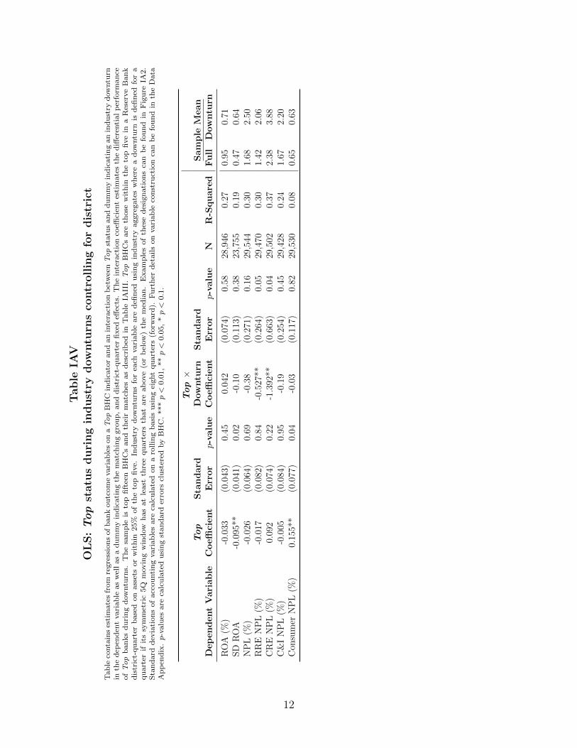


![OnAngular Correlations and HighEnergyEvolution. · arXiv:1109.0347v1 [hep-ph] 2 Sep 2011 OnAngular Correlations and HighEnergyEvolution. Alex Kovner 1and Michael Lublinsky2, 1 Physics](https://static.documents.pub/doc/80x56/5f87dc594f3fe737e52127d6/onangular-correlations-and-arxiv11090347v1-hep-ph-2-sep-2011-onangular-correlations.jpg)


