Page 1
Beyond Contiguity: The Role of Temporal Distributions
and Predictability in Human Causal Learning
A dissertation submitted to the School of Psychology, Cardiff University,
in partial fulfilment of the requirements for the degree of
Doctor of Philosophy
September, 2011
by
James Greville
School of Psychology Cardiff University
Tower Building
Park Place
CF10 3AT
Cardiff, UK
Page 2
ii
Abstract
Most contemporary theories of causal learning identify three primary cues to causality;
temporal order, contingency and contiguity. It is well-established in the literature that a lack of
temporal contiguity – a delay between cause and effect – can have an adverse effect on causal
induction. However research has tended to focus almost exclusively on the extent of delay while
ignoring the potential influence of delay variability. This thesis aimed to address this oversight.
Since humans tend to experience causal relations repeatedly over time, we accordingly
experience multiple cause-effect intervals. If intervals are constant, it becomes possible to predict
when the effect will occur following the cause. Fixed delays thus confer temporal predictability,
which may contribute to successful causal inference by creating an impression of a stable
underlying mechanism. Five experiments confirmed the facilitatory effect of predictability in
instrumental causal learning. Two experiments involving a different aspect of causal judgment
found no effects of interval variability, but two further experiments demonstrated that
predictability facilitates elemental causal induction from observation. These results directly
conflict with findings from studies of animal conditioning, where preference for variable- interval
reinforcement is routinely exhibited, and a simple associative account struggles to explain this
disparity. However both a temporal coding associative account, and higher-level cognitive
perspectives such as Bayesian structural inference, are compatible with these findings. Overall,
this thesis indicates that causal learning involves processes above and beyond simple
associations.
Page 3
iii
Preface
This thesis was completed at the School of Psychology, Cardiff University, under the supervision
of Dr. Marc Buehner, 2007-2011.
Parts of the empirical work in Chapter 3, specifically experiments 1, 2B and 3, were published in
the article: Greville, W. J., & Buehner, M. J. (2010) Temporal Predictability Facilitates Causal
Learning. Journal of Experimental Psychology: General, 139(4), 756–771. Other work
undertaken during this period of study, but not presented in this thesis, is currently being revised
for publication in Memory & Cognition.
An overview of this research was presented at the following conferences:
BPS Cognitive Section Annual Conference, September 2009: University of Hertfordshire, UK;
1st joint meeting of EPS and SEPEX: April 2010, Granada, Spain; 36th Annual Convention of
the Association for Behavior Analysis: June 2010, San Antonio, Texas; BPS Cognitive Section
Annual Conference, September 2010: Cardiff University, UK.
This research was supported by a grant from the Engineering and Physical Sciences Research
Council (EPSRC).
Page 4
iv
Acknowledgements
Firstly, immense thanks are due to my supervisor Marc Buehner. His careful guidance
struck just the right balance between giving me the freedom to develop my own interests whilst
still keeping me focused. I will always be very grateful for his continual encouragement along an
often arduous but ultimately enjoyable journey.
I thank Cardiff University and the EPSRC for generously funding my research.
I would also like to thank my friends and collaborators at Cardiff University, in particular
my second supervisor Mark Johansen, Adam Cassar, Sindhuja Sankaran, and Laurel Evans.
I thank Anthonia for countering my melancholia with her warmth and vivacity.
Finally I would like to thank my family and especially my sister, Katharine, and my
parents, David and Maureen, for their enduring love and support.
Dedication
This thesis is dedicated to the memory of three dearly missed people that sadly departed
during the past three years:
To my grandpa, Norman Gordon, a kind and caring man of true integrity, who proudly
served his country and who loved and was loved by his family.
To my friend, Quirine Charlton-Robbins, whose bravery in the face of adversity was
incredible and whose cheer and generosity is missed by all those who knew her.
Finally to Christopher Douglas Brown, one of my oldest and dearest friends, who genuinely
inspired me with his courage and determination to follow his own path in his own way, and
showed that richness of experience rather than accumulation of years is the true measure of life.
Page 5
v
Table of Contents
ABSTRACT ........................................................................................................................................................................iii
PREFACE............................................................................................................................................................................iii
ACKNOWLEDGEMENTS AND DEDICATION.....................................................................................................iv
LIST OF FIGURES ............................................................................................................................................................x
LIST OF TABLES ...............................................................................................................................................................x
CHAPTER 1 – CURRENT PERSPECTIVES ON CAUSAL LEARNING ........................................................1
1.1 CAUSALIT Y AND CAUSAL LEARNING – A BRIEF INTRODUCTION........................................................................1 1.2 THE CENTRAL PROBLEM FOR CAUSAL LEARNING ..................................................................................................1 1.3 PLAN OF THE THESIS...................................................................................................................................................3 1.4 HUME’S CUES T O CAUSALIT Y ..................................................................................................................................4
1.4.1 Temporal Order.................................................................................................................................................4 1.4.2 Contingency........................................................................................................................................................4 1.4.3 Contiguity ...........................................................................................................................................................6
1.5 THEORIES OF CAUSAL LEARNING............................................................................................................................9 1.5.1 Conditioning and Associative Learning Theory ....................................................................................... 10
1.5.1.1 The Rescorla-Wagner M odel......................................................................................................................11 1.5.1.2 The Role of Time from an Associative Perspective ...................................................................................13 1.5.1.3 Difficulties for an Associative Account of Causality Judgment.................................................................15
1.5.2 Causal Mechanism and Power Theories.................................................................................................... 16 1.5.2.1 The Power PC Theory.................................................................................................................................17 1.5.2.2 The Role of Time from Covariation Perspectives ......................................................................................18
1.5.3 Causal Models and Structure Theories...................................................................................................... 20 1.5.3.1 Causal M odel Theory..................................................................................................................................21 1.5.3.2 Bayesian Structure Learning.......................................................................................................................23 1.5.3.3 Causal Support............................................................................................................................................24 1.5.3.4 A Bayesian Perspective on Contiguity........................................................................................................25
1.5 CHAPT ER SUMMARY................................................................................................................................................27
CHAPTER 2 – THE POTENTIAL ROLE OF TEMPORAL PREDICTABILITY IN CAUSAL LEARNING................................................................................................................................................................................................ 30
2.1 INT RODUCING TEMPORAL PREDICTABILITY.........................................................................................................30 2.2. THE TEMPORAL PREDICTABILITY HYPOTHESIS..................................................................................................32 2.3 PREVIOUS EMPIRICAL RESEARCH ON PREDICTABILITY......................................................................................34 2.4 ANIMAL PREFERENCE FOR VARIABLE REINFORCEMENT....................................................................................35 2.5 THEORETICAL PERSPECTIVES ON PREDICTABILITY.............................................................................................37
2.5.1 An Associative Analysis of Temporal Predictability................................................................................ 37 2.5.2 The Attribution Shift Hypothesis.................................................................................................................. 41 2.5.3 Bayesian Models ............................................................................................................................................ 42
2.6 CHAPT ER SUMMARY................................................................................................................................................44
CHAPTER 3 – THE ROLE OF TEMPORAL PREDICTABILITY IN INSTRUMENTAL CAUSAL
LEARNING........................................................................................................................................................................ 46
3.1 OVERVIEW AND INTRODUCTION.............................................................................................................................46 3.2 EXPERIMENT 1...........................................................................................................................................................47
3.2.1 Method ............................................................................................................................................................. 49 3.2.1.1 Participants..................................................................................................................................................49 3.2.1.2 Design .........................................................................................................................................................49 3.2.1.3 Apparatus, Materials and Procedure ...........................................................................................................51
3.2.2 Results.............................................................................................................................................................. 52
Page 6
vi
3.2.2.1 Causal Judgments........................................................................................................................................52 3.2.2.2 Instrumental Behaviour and Outcome Patterns ..........................................................................................55
3.2.3 Discussion ....................................................................................................................................................... 57 3.3 EXPERIMENT 2A .......................................................................................................................................................58
3.3.1 Method ............................................................................................................................................................. 59 3.3.1.1 Participants..................................................................................................................................................59 3.3.1.2 Design .........................................................................................................................................................60 3.3.1.3 Apparatus, materials & procedure ..............................................................................................................61
3.3.2 Results & Discussion..................................................................................................................................... 61 3.3.2.1 Causal Ratings.............................................................................................................................................61 3.3.2.2 Behavioural Data.........................................................................................................................................63
3.2.3 Discussion ....................................................................................................................................................... 63 3.3 EXPERIMENT 2B........................................................................................................................................................64
3.3.1 Method ............................................................................................................................................................. 66 3.3.1.1 Participants..................................................................................................................................................66 3.3.1.2 Design .........................................................................................................................................................66 3.3.1.3 Apparatus, Materials & Procedure..............................................................................................................67
3.3.2 Results.............................................................................................................................................................. 67 3.3.2.1 Causal Ratings.............................................................................................................................................67 3.3.2.2 Instrumental Behaviour and Outcome Patterns ..........................................................................................68 3.3.3 Discussion......................................................................................................................................................69
3.4 EXPERIMENT 3...........................................................................................................................................................71 3.4.1 Method ............................................................................................................................................................. 72
3.4.1.1 Participants..................................................................................................................................................72 3.4.1.2 Design .........................................................................................................................................................72 3.4.1.3 Apparatus, materials & procedure ..............................................................................................................73
3.4.2 Results.............................................................................................................................................................. 73 3.4.2.1 Causal Ratings.............................................................................................................................................73 3.4.2.2 Instrumental Behaviour and Outcome Patterns ..........................................................................................74 3.4.3 Discussion......................................................................................................................................................75
3.5 EXPERIMENT 4...........................................................................................................................................................76 3.5.1 Overview of experiment.................................................................................................................................77 3.5.2 Predictions......................................................................................................................................................78
3.5.3 Method ............................................................................................................................................................. 78 3.5.3.1 Participants..................................................................................................................................................78 3.5.3.2 Design .........................................................................................................................................................78 3.5.3.3 Apparatus& M aterials .................................................................................................................................79 3.5.3.4 Procedure ....................................................................................................................................................79
3.5.4 Results.............................................................................................................................................................. 79 3.5.4.1 Causal Judgments........................................................................................................................................79 3.5.4.2 Instrumental Behaviour and Outcome Patterns ..........................................................................................80
3.5.5 Discussion ....................................................................................................................................................... 81 CHAPTER SUMMARY.......................................................................................................................................................83
CHAPTER 4 – THE ROLE OF TEMPORAL PREDICTABILITY IN OBSERVATIONAL CAUSAL
LEARNING........................................................................................................................................................................ 84
4.1 PARALLELS AND DISPARITIES BETWEEN CLASSICAL AND INST RUMENTAL CONDITIONING.........................85 4.2 DIST INGUISHING INTERVENTION AND OBSERVATION.........................................................................................86 4.3 EXI ST ING EVIDENCE – YOUNG & NGUYEN, 2009 ...............................................................................................88
4.3.1 An alternative to the predictability hypothesis – The temporal proximity account........................... 90 4.3.2 The video game context................................................................................................................................. 92
4.4 EXPERIMENT 4A .......................................................................................................................................................92 4.4.1 Predictions ...................................................................................................................................................... 94 4.4.2 Speed-Accuracy Tradeoff.............................................................................................................................. 94 4.4.3 Method ............................................................................................................................................................. 95
4.4.3.1 Participants and Apparatus..........................................................................................................................95 4.4.3.3 Design and Materials ..................................................................................................................................96 4.4.3.4 Procedure ....................................................................................................................................................97
4.4.4 Results.............................................................................................................................................................. 99 4.4.4.1 Speed-Accuracy Tradeoff .........................................................................................................................100 4.4.4.2 Sampling Time ..........................................................................................................................................101
Page 7
vii
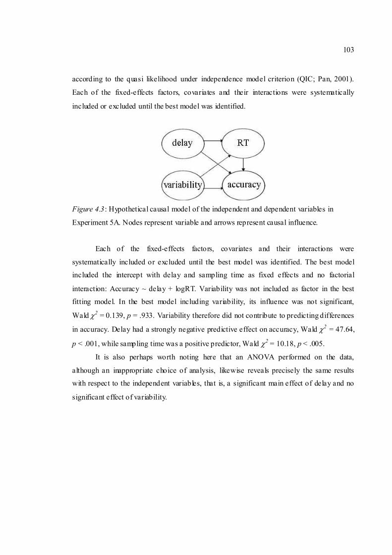
4.4.4.3 Accuracy ...................................................................................................................................................102 4.4.5 Discussion .....................................................................................................................................................104
4.5 EXPERIMENT 5B......................................................................................................................................................108 4.5.1 Method ...........................................................................................................................................................109
4.5.1.1 Participants................................................................................................................................................109 4.5.1.2 Design .......................................................................................................................................................109 4.5.1.3 Apparatus & M aterials ..............................................................................................................................110 4.5.1.4 Procedure ..................................................................................................................................................110
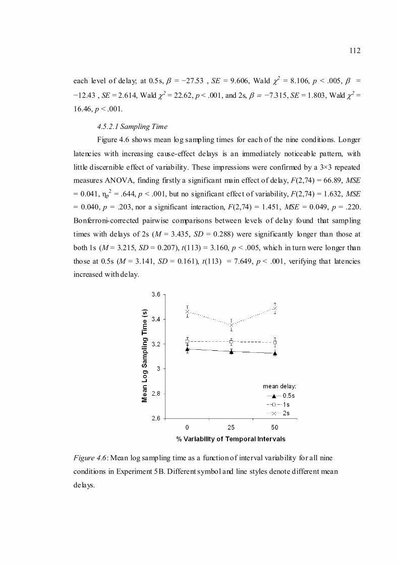
4.5.2 Results............................................................................................................................................................111 4.5.2.1 Sampling Time ..........................................................................................................................................112 4.5.2.2 Accuracy ...................................................................................................................................................113
4.5.3 Discussion .....................................................................................................................................................114 4.5.3.1 A Speed-Accuracy Violation ....................................................................................................................114 4.5.3.2 Failure to find support for predictability...................................................................................................115 4.5.3.3 Temporal order violations may reveal the true cause ...............................................................................117 4.5.3.4 Alternative Applications ...........................................................................................................................119 4.5.3.5 “Back to Basics” .......................................................................................................................................119
4.6 EXPERIMENT 6A .....................................................................................................................................................121 4.6.1 An Observational Analogue of the Elemental Causal Judgment Task ...............................................122 4.6.2 Method ...........................................................................................................................................................124
4.6.2.1 Participants................................................................................................................................................124 4.6.2.2 Design .......................................................................................................................................................124 4.6.2.3 Apparatus, Materials and Procedure .........................................................................................................124
4.6.3 Results............................................................................................................................................................126 4.6.3.1 Causal Ratings...........................................................................................................................................126 4.6.3.2 Cue and outcome patterns.........................................................................................................................127
4.6.4 Discussion .....................................................................................................................................................130 4.7 EXPERIMENT 6B......................................................................................................................................................134
4.7.1 Method ...........................................................................................................................................................134 4.7.1.1 Participants................................................................................................................................................134 4.7.1.3 Apparatus, Materials & Procedure............................................................................................................135
4.7.2 Results............................................................................................................................................................135 4.7.2.1 Causal Ratings...........................................................................................................................................135 4.7.2.2 Cue and outcome patterns.........................................................................................................................136 4.7.3 Discussion....................................................................................................................................................137
4.8 CHAPT ER SUMMARY..............................................................................................................................................140
CHAPTER 5 – GENERAL DISCUSSION AND CONCLUSIONS .................................................................141
5.1 BRIEF SYNOPSIS OF EXPERIMENTS.......................................................................................................................141 5.2 TEMPORAL PREDICTABILITY FACILIT ATES ELEMENTAL CAUSAL INDUCTION.............................................142 5.3 AN ASSOCIATIVE ANALYSIS OF TEMPORAL PREDICTABILITY.........................................................................144
5.3.1 Delay Discounting........................................................................................................................................145 5.3.2 The Temporal Coding Hypothesis.............................................................................................................148
5.4. A CONTINGENCY-BASED PERSPECTIVE ON PREDICTABILITY...........................................................................150 5.4.1 Attribution Aide or Cognitive Component?.............................................................................................152
5.5 A BAYESIAN ACCOUNT OF PREDICT ABILITY.......................................................................................................152 5.6 A NOVEL APPROACH – TEMPORAL EXPECT ANCY THEORY.............................................................................153 5.7 MET HODOLOGICAL CONCERNS ............................................................................................................................156
5.7.1 Interactions of Predictability with Delay Extent and Background Effects.........................................157 5.8 FUT URE DIRECTIONS..............................................................................................................................................158 5.9 CONCLUSIONS .........................................................................................................................................................160
REFERENCES ................................................................................................................................................................163
Page 8
viii
List of Figures
Figure 1.1: Standard 2×2 contingency matrix, showing the four possible combinations of cause
and effect occurrence and non-occurrence..............................................................................6
Figure 1.2: The effect of attribution shift in parsing an event stream with a specific timeframe
assumed : c � e intervals that are longer than the temporal window simultaneously decrease
impressions of P(e|c) and P(¬e|¬c) while increasing impressions of P(e|¬c) and P(¬e|c). 19
Figure 1.3: Directed acyclic graph representing causal influence of X on Y.......................20
Figure 1.4: Directed acyclic graphs representing the two basic hypotheses that are compared in
elemental causal induction....................................................................................................24
Figure 2.1: Potential differences in accrued associative strength between fixed- interval and
variable-interval conditions according to a hyperbola- like discounting function of delayed events.
...............................................................................................................................................40
Figure 3.1: Diagram representing the three types of temporal distribution applied in Experiment 1
at the two levels of mean delay. ............................................................................................51
Figure 3.2: Mean Control Ratings for all conditions in Experiment 1 as a function of background
effects. Filled and unfilled symbols refer to mean delays of 2s and 4s respectively. Delay
variability is noted by different symbol and line styles. Error bars are omitted for clarity. .53
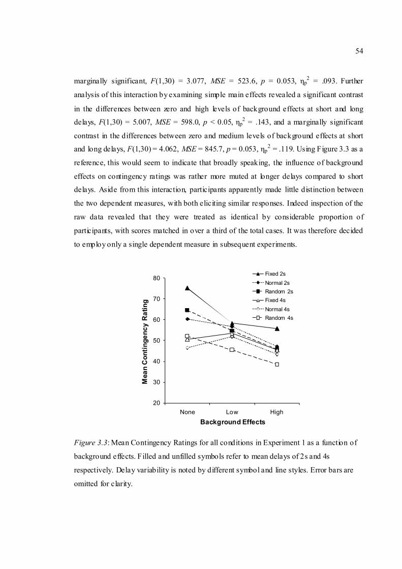
Figure 3.3: Mean Contingency Ratings for all conditions in Experiment 1 as a function of
background effects. Filled and unfilled symbols refer to mean delays of 2s and 4s respectively.
Delay variability is noted by different symbol and line styles. Error bars are omitted for clarity.
...............................................................................................................................................54
Figure 3.4: Diagram illustrating the combination of the levels Delay and Range to produce the
six experimental conditions in Experiment 2A.....................................................................60
Figure 3.5: Mean Causal Ratings from Experiment 2A as a function of temporal interval range.
Different symbol and line styles represent different delays. Error bars show standard errors.62
Page 9
ix
Figure 3.6: Mean Causal Ratings from Experiment 2B as a function of interval range. Filled and
unfilled symbols refer to master and yoked conditions respectively. Mean delays are noted by
different symbol and line styles. ...........................................................................................68
Figure 3.7: Mean Causal Ratings from Experiment 3 as a function of interval range. Filled and
unfilled symbols refer to 2 and 4 minutes training respectively. Mean delays are noted by
different symbol and line styles. ...........................................................................................74
Figure 3.8: Mean causal ratings from Experiment 4 as a function of P(e|c). Filled and unfilled
symbols refer to fixed and variable delays respectively. ......................................................80
Figure 4.1: Screen shot of the stimuli used in Experiments 5A and 5B...............................98
Figure 4.1: Scatter plot showing participants’ mean percentage accuracy as a function of their
mean log sampling time across all nine conditions in Experiment 5A. ..............................101
Figure 4.2: Mean log sampling time as a function of interval variability for all nine conditions in
Experiment 5A. Different symbol and line styles denote different mean delays. Error bars show
standard errors.....................................................................................................................102
Figure 4.3: Hypothetical causal model of the independent and dependent variables in Experiment
5A. Nodes represent variable and arrows represent causal influence.................................103
Figure 4.4: Mean percentage accuracy as a function of delay variability for all nine conditions in
Experiment 5A. Different symbol and line style refer to different mean delays. Error bars are
omitted due to the dichotomous nature of the dependent measure. ....................................104
Figure 4.5: Scatter plot showing participants’ mean percentage accuracy as a function of their
mean log sampling time across all nine conditions in Experiment 5B. ..............................111
Figure 4.6: Mean log sampling time as a function of interval variability for all nine conditions in
Experiment 5B. Different symbol and line styles denote different mean delays................112
Figure 4.7: Mean percentage accuracy as a function of interval variability for all nine conditions
in Experiment 5B. Different symbol and line styles denote different mean delays. ..........113
Page 10
x
Figure 4.8: Mean causal ratings as a function of temporal interval range for all six conditions in
Experiment 6A. Different symbol and line styles denote different mean delays. ..............127
Figure 4.9: Mean causal ratings for Experiment 6B as a function of temporal interval range.
Different symbol and line styles denote different mean delays. Error bars show standard errors.
.............................................................................................................................................137
List of Tables
Table 3.1: Behavioural Data for Experiment 1. Standard deviations are given in parentheses.
...............................................................................................................................................56
Table 3.2: Behavioural Data for Experiment 2A. Standard deviations are given in parentheses.
...............................................................................................................................................62
Table 3.3: Behavioural Data for Experiment 2B. Standard deviations are given in parentheses.
...............................................................................................................................................69
Table 3.4: Behavioural Data for Experiment 3. Standard deviations are given in parentheses.
...............................................................................................................................................75
Table 3.5: Behavioural Data for Experiment 4. Standard deviations are given in parentheses.
...............................................................................................................................................81
Table 4.1: Behavioural data for Experiment 6A. Standard deviations are given in parentheses.
.............................................................................................................................................128
Table 4.2: Behavioural data for Experiment 6B. Standard deviations are given in parentheses.
.............................................................................................................................................138
Page 11
1
Chapter 1 – Current Perspectives on Causal Learning
1.1 Causality and Causal Learning – A brief introduction
The study of causality has a long and rich history in both philosophy and
psychology. In essence, causality is understood as the relationship between one event or
entity, the cause, and another event or entity, the effect, such that the second is recognized
to be a consequence of the first. In other words, causes produce or generate effects. Causal
learning, in the simplest sense, is how we come to learn that one thing causes another.
An expanded and more precise definition of causality acknowledges that causes
may be either deterministic, where the effect necessarily follows from the cause, or
probabilistic, where the cause alters the likelihood of the effect. Furthermore, causes may
be generative, producing or increasing the probability of occurrence of an outcome, or
preventative, inhibiting an outcome that would otherwise have occurred. Causality then
may be seen as the underlying laws that govern systematic relations between events.
Multiple relationships between multiple entities or events may exist within a given
system. For example, a fire may produce smoke and heat, both of which are common
effects, while the fire itself may have resulted from natural causes (such as a bolt of
lightning) or from deliberate human action, both of which may be regarded as common
causes (or parents). Such an interconnected series of events is known as a causal network
(Pearl, 2000). Causal learning may thus be more broadly defined as the process by which
we construct and represent causal relations and networks, and how we use this information
in thinking, reasoning, judgment and decision-making. The research presented within this
thesis however focuses on the former, more fundamental question of causal learning – how
do humans learn that one thing causes another?
1.2 The central problem for causal learning
The ability to learn enables us to adapt to our environment and, ultimately, to
survive. If learning has evolved as an adaptive mechanism, it is natural that the content of
learning should reflect relations that actually exist in the universe (Shanks, 1995). Causal
learning endows us with the capacity to create representations that mirror the causal
structure of our surrounding environment. Creating such representations allows us to
Page 12
2
understand how and why events occur, to predict the occurrence of future events, and to
intervene on the world and control our environment, directing our behaviour to evoke
desired consequences and achieve goals. Causal learning is thus a core cognitive capacity
and a crucial adaptive mechanism. The central question for learning theorists interested in
causality is how such knowledge is acquired.
Seeking an answer to this question has been a preoccupation of scholars throughout
the ages. Yet, this may, to the uninitiated, seem somewhat surprising. When asked “how do
you learn that one thing causes another?” an immediate answer may spring to mind such as
“I see it happen and so I know how it works” (Schlottmann, 1999). One might then be
puzzled as to why this question has provided such a dilemma when the answer seems so
intuitively obvious. For example, when one kicks a ball, the causal connection between so
doing and the subsequent motion of the ball seems immediately apparent. Indeed, it has
been argued that such events involving physical collision of objects or “launching”
(Michotte, 1946/1963) may indeed give rise to direct causal perception (for an overview see
Scholl & Tremoulet, 2000).
Consider however some alternative examples. When one practices a skill such as
learning a musical instrument, there is typically a causal understanding that continued
practice will lead to improved performance. However we cannot directly see the
physiological changes to the neurons in the brain and muscle fibres in the body that practice
confers to improve the co-ordination and dexterity of the individual. Nor can the cellular
changes be observed when, for instance, a pathogen invades our body and causes illness, or
a drug is taken to treat that illness and eliminate the pathogen from our system. How then,
have we come to learn causal relations such as that microscopic pathogens cause illness and
that certain drugs will eradicate these unwanted visitors, or that one can develop a skill
through practice?
Such unobservable causal relations need not always involve biological processes.
Hanging a wet cloth outside on a sunny day, for instance, will cause the cloth to dry, and
we may well be able to observe the cloth becoming drier, if we have nothing better to do.
What we cannot see however, is the mechanism involved, the transfer of energy, the water
molecules becoming more excited and eventually changing state from liquid to vapour as
they evaporate from the cloth. Moreover, we cannot directly perceive the laws of physics
Page 13
3
governing the behaviour of molecules, such as in the evaporation of water, which
ultimately underpin this process. Such causal laws or relations are not entities in themselves
and are therefore imperceptible; we cannot see (nor hear, touch, smell or taste) a causal law.
If such laws are unobservable, then how can we ever become aware of them?
Although philosophical concerns regarding causality extend as far back as the days
of Aristotle, it was the Scottish empiricist David Hume (1711-1776) that first formalized
and addressed the “riddle of induction” that is exemplified by such scenarios as described
above. Hume reasoned that since our sensory modalities are not attuned to the detection of
causality per se, the existence of causal relations can only be inferred from the observable
evidence that is accessible to us (Hume, 1739/1888). Causal learning is therefore often
referred to also as causal inference or induction. It follows then that representations of
causal relations must be constructed on the basis of the sensory input we receive from the
world around us. Hume proposed that there are crucial ‘cues to causality’ that underpin
such representations, and identified the most important determinants as 1) temporal order –
causes must precede their effects; 2) contingency – effects must repeatedly and reliably
follow their causes; and 3) contiguity – causes and effects must be closely connected in
space and time.
These statistical and temporal relations between events form the bedrock of nearly
all theories of causal learning. The primary goal of this thesis is to address the possibility of
an additional cue, namely temporal predictability, contributing to the process of causal
inference. At this point then, it seems appropriate to provide a brief overview of the thesis,
and outline how this question shall be approached.
1.3 Plan of the thesis
The remainder of this chapter will firstly explore in more detail each of the cues to
causality as suggested by Hume, and the role each is considered to play in causal learning.
Following this, I shall briefly introduce three broad theories of causal learning, each of
which has its own particular interpretation of how humans and other agents use such cues
to learn about causal relations. This background is necessary for the eventual evaluation of
the empirical results that will be presented further on. Chapter 2 then fully introduces this
concept of temporal predictability and outlines how such a feature might be a factor in
Page 14
4
causal learning. It is then considered how each of the theories of causal learning introduced
in Chapter 1 might accommodate any effects of this potential cue of temporal predictability
that may be subsequently identified. Chapters 3 and 4 then provide a series of experiments
designed to assess the empirical contribution of temporal predictability, in both
instrumental and observational learning tasks. Finally, Chapter 5 provides a full discussion
of these results and considers their implications, as well as suggesting a new abstract model
to account for these results, before concluding the thesis by looking towards future research
that might be pursued along this same vein.
1.4 Hume’s Cues to Causality
1.4.1 Temporal Order
Hume’s first cue of temporal order is perhaps the most fundamental, and its
importance is almost unanimously accepted across researchers; causes must occur prior to
the effects they produce. There are however a few notable clauses in this dictum. Firstly,
events may not always be observed in their causal order (see Waldmann & Holyoak, 1992).
For instance, during a medical diagnosis, a physician may detect a symptom before
identifying the disease that is causing it. Such situations are in fact crucial for
distinguishing between the predictions of different theories of causal learning, as shall be
discussed in more detail further on in this thesis. Secondly, research has shown that new
information can influence the perception of events in the past, in what is known as
postdictive perception (Choi & Scholl, 2006). Nevertheless, in most contemporary accounts
of causal learning, temporal order is taken as a given necessity for causal inference.
1.4.2 Contingency
The vast majority of the literature on causal learning has focused on the second cue
of contingency, and how this information may be used to infer causality. Contingency is the
extent to which the effect is dependent (contingent) upon the cause, or in other words, the
degree of covariation between cause and effect. This encompasses both the extent to which
the effect follows the cause, and also the extent to which the effect occurs without the
cause, known as the base rate. Contingency then is the degree of statistical dependency
between the presence and absence of candidate causes and their putative effects.
Page 15
5
While of course both causes and effects may take the form of stimuli whose
properties are on a continuum (such as the brightness of a light or the loudness of a tone),
most models of causal learning simplify the problem by defining cause and effect as either
present or absent. Researchers generally agree that the statistical information we receive
with regard to the presence or absence of candidate causes and effects is computed in some
way to assess the covariation between them, which can then form the basis for a causal
judgment. At the root of most covariation models is the 2×2 contingency matrix, as shown
in Figure 1.1, which describes in the most simple format the possible combinations in
which cause and effect can be either present or absent. Exactly how this information is
computed is still the subject of rigorous debate (Buehner, Cheng, & Clifford, 2003; Cheng,
1997; Cheng & Novick, 2005; Lober & Shanks, 2000; Luhmann & Ahn, 2005; White,
2005) and numerous models with varying degrees of complexity have been proposed to
account for this computation.
One of the best known and widely used models is the ∆P statistic (Jenkins & Ward,
1965). In fact such is the popularity of this measure that it is often treated as an objective
measure of contingency and “contingency” is sometimes used as a synonym for ∆P. The
value of ∆P is given by the difference between the probability of the effect in the presence
of the cause, P(e|c), and the probability of the effect in the absence of the cause, P(e|¬c). In
terms of the cells of the contingency matrix, this is calculated as:
∆P = P(e|c) – P(e|¬c) = A/(A+B) – C(C+D)
There are of course different ways in which the cells of the table may be combined,
including among others the ∆D rule, calculated as (A+B) – (C+D). For an overview of a
number of such rules, see Hammond and Paynter (1983). More recently developed models,
for instance Cheng’s (1997) Power PC theory, have extended covariation-based models to
account for some of the particular phenomena of causal inference that ∆P alone cannot
represent. While the discourse continues over how covariation information is and should be
utilized in making causal inferences, all researchers would likely agree with the general
principle that the greater the contingency between cause and effect, the stronger the
perception of causality.
Page 16
6
Figure 1.1: Standard 2×2 contingency matrix, showing the four possible combinations of
cause and effect occurrence and non-occurrence.
1.4.3 Contiguity
The second of Hume’s tenets, contiguity, refers to the proximity of the cause and
effect both in space and in time – spatial and temporal contiguity. In a classic illustration of
the importance of contiguity, Michotte (1946/1963) used simple visual stimuli to
demonstrate the “launching” effect. A prototypical procedure began with two squares (X
and Y) separated from each other by a small distance. X then began to move in a straight
line towards Y. On reaching Y (so that their outer surfaces appear to make contact), X
stopped moving and Y immediately began to move along the same trajectory. Such a
sequence created the strong impression that X collided with Y and caused Y to move.
Reports from Michotte’s participants revealed that if Y began to move only after a delay
(lack of temporal contiguity), or before it was reached by X (lack of spatial contiguity), the
causal impression of X having launched Y was destroyed.
However, as alluded to earlier, a distinction may be drawn between causal
perception, which involves a direct interaction and visible physical contact between the
participants in the causal relation, and causal induction, when the physical interaction
between participants is undetectable and the relation must instead be inferred (Cavazza,
Lugrin, & Buehner, 2007; Schlottmann & Shanks, 1992; Scholl & Nakayama, 2002). While
spatial contiguity remains of utmost importance for perceptual causality (as in the above
example of launching), in the case of causal induction (such as in the earlier example of
inferring the causes of disease), the necessity of spatial contiguity tends to be downplayed.
After all, many events can often be triggered remotely, such as flipping a switch at one end
Page 17
7
of a room to cause a light to come on at the other end. Most contemporary research on
causal inference instead then focuses on temporal rather than spatial contiguity.
Relatively speaking, there has been far less empirical attention devoted to contiguity
compared to contingency (although the disparity is gradually being redressed in recent
years). As a result, contiguity is less well understood and its role in causal learning more
uncertain. According to Hume, contiguity between cause and effect is essential to the
process of causal induction. This supposition was affirmed in a systematic investigation by
Shanks, Pearson and Dickinson (1989). Their task involved judging how effective pressing
the space-bar on a keyboard was in causing a triangle to flash on a computer screen.
Participants were given a fixed amount of time to engage on the task and could gather
evidence through repeatedly pressing the space-bar and observing whether or not the
outcome occurred. The apparatus was set up to deliver the outcome with a 0.75 probability
when the space-bar was pressed. On each trial, if an outcome was scheduled, it would occur
after a specific amount of time following the space-bar. This interval varied between
conditions from 0 up to 16s. It was found that as the delay increased, participants’ causal
judgments decreased in systematic fashion. In fact, conditions involving delays of more
than 2s were no longer distinguished as causally effective and were judged just as
ineffective as non-contingent control conditions.
Shanks et al.’s (1989) results provided evidence that delays have a deleterious effect
on impressions of causality, corroborating the assertions of Hume that contiguity is indeed
necessary for causal learning. Yet this idea seems at odds with everyday cognition. Humans
and other animals often demonstrate the ability to correctly link causes and effects that are
separated in time and learn causal relations involving delays of considerable length; over
days, weeks, even months at a time – an often cited example is the temporal gap between
intercourse and birth (Einhorn & Hogarth, 1986). And yet, Shanks et al. show a failure to
detect causal relations involving gaps of more than a few seconds. Clearly there must be
something that enables us to bridge such temporal gaps and infer delayed causal relations.
Einhorn & Hogarth (1986) proposed a knowledge mediation hypothesis. They argue
that rather than being essential, the function of contiguity is as a cue to direct attention to
the contingencies between events. According to this view, people can overcome the
requirement for events to be contiguous if there is some other reason why an attentional
Page 18
8
link should form between these events; for example, if they have knowledge of some
existing mechanism that may connect one to the other. Some knowledge of human biology
might therefore enable the connection between intercourse and birth. According to this
view, if there is an expectation for a delayed mechanism, a temporal delay no longer
becomes an obstacle to causal inference. Thus prior knowledge can mediate the impact of
temporal delays.
Adopting this perspective, Buehner and May (2002) demonstrated the detrimental
effect of delay could be mitigated by invoking high- level knowledge in participants. In
judgment tasks where a cover story was used to make a delay between cause and effect
seem plausible (the effect was an explosion and the candidate cause was the launching of a
grenade), causal ratings were significantly less adversely affected by delays compared to
situations where the cover story made delay seem implausible (where the effect was a
lightbulb illuminating and the candidate cause was pressing a switch). Further work by
Buehner and May (2004) showed that the effect of delay could be abolished completely by
providing explicit information regarding the expected timeframe of the causal relation.
Participants again evaluated the effectiveness of pressing a switch on the illumination of a
lightbulb; however one group of participants were told that the bulb was an ordinary bulb
that should light up right away, while another group of participants was instructed that the
bulb was an energy-saving bulb that lights up after a delay. For this latter group there was
no decline in ratings with delay; delayed and immediate causal relations were judged as
equally effective. Indeed in some circumstances, delays even may serve to facilitate causal
attribution where an immediate consequence is incompatible with an expected mechanism
(Buehner & McGregor, 2006).
Additionally, Buehner and May (2003) also found that mediation of delay could
also be induced through prior experience; they found strong order effects such that where
conditions with immediate causal relations preceded conditions with delayed relations,
causal ratings were markedly lower compared to when delayed causal relation conditions
were presented first. Reed (1992) and Young, Rogers and Beckmann (2005) show that
filling an interval with a stimulus such as an auditory tone (known as “signalling”) can
likewise negate the impact of delays. Greville, Cassar, Johansen, and Buehner (2010) have
meanwhile shown that delays of reinforcement no longer impair instrumental learning
Page 19
9
when the task environment highlights the underlying contingency structure. Such work
provides insight as to how causal inference can take place over longer time periods.
Nevertheless, most researchers agree that in the absence of such mitigating information as
described above, delays tend to have a deleterious effect on causal learning, and temporal
contiguity thus remains an important cue to causality. Barring a few exceptions, all other
things being equal, contiguous causes and effects elicit a stronger causal impression than
causes and effects separated by a delay.
1.5 Theories of Causal Learning
Despite a fairly general consensus over the importance of Hume’s cues to causality,
there is considerable disagreement with regard to the processes that underlie causal
inference. Moreover, no model of learning thus developed has thus provided a full account
of causal learning that encompasses its various idiosyncrasies. Dissatisfaction with existing
accounts has led to the development of a veritable smorgasbord of learning rules and
models over the years, some with the intention of addressing specific facets of learning that
previous efforts could not account for, and some providing a more general framework.
Each is motivated from a particular theoretical stance, and each has had its successes and
shortcomings debated, some more favourably so than others. One long-standing measure,
∆P, has already been briefly described. Others include the probabilistic contrast model
(Cheng & Novick, 1990); Power PC (Cheng, 1997); the pCI rule (White, 2003); BUCKLE
(Luhmann & Ahn, 2007); knowledge-based causal induction (Waldmann, 1996); causal
support (Griffiths & Tenenbaum, 2005); and theory-based causal induction (Griffiths &
Tenenbaum, 2009). While these examples specifically address human causal learning,
models of animal conditioning have also been applied (with varying degrees of success) to
account for causal inference, including the Rescorla-Wagner model (1972); the SOP model
(Wagner, 1981); the Pearce-Hall (1980) and Pearce (1987) models; scalar expectancy
theory (Gibbon, 1977); and rate estimation theory (Gallistel & Gibbon, 2000b). Neither of
these lists are exhaustive and it is of course unfeasible to accommodate a detailed
explanation of all existing models of causal learning within this thesis. Indeed, a full
account of a single more complex framework such as theory-based causal induction could
easily stand alone as a doctoral thesis in itself (see, e.g., Griffiths, 2005). Instead it seems
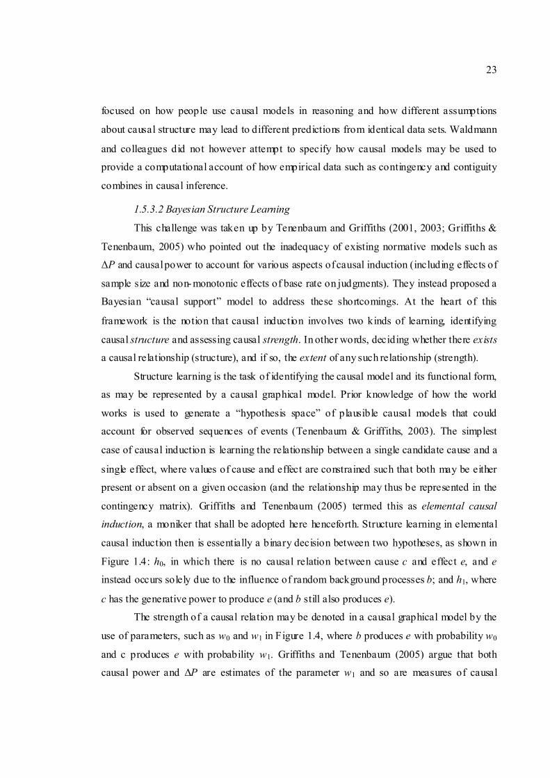
Page 20
10
more appropriate to categorise these models based on their common ground, and consider
the general principles underlying each particular theoretical position. It is also worthwhile
to point out at this juncture that the work contained in this thesis examines only generative
causes. Accordingly the following review of existing models of causal learning will focus
on the generative form.
1.5.1 Conditioning and Associative Learning Theory
Learning in animals is measured by changes in behaviour. Indeed, it has been
argued that learning is, by definition, a change in behaviour and that such changes are the
only way by which learning can be measured (Baum, 1994). Stimuli that elicit a change in
the behaviour of an organism may be categorized as either reinforcers, which increase the
frequency of a behaviour, or punishments, which decrease the frequency of a behaviour.
The common conception of reinforcement or punishment is the delivery of a stimulus that
has a particular motivational significance or adaptive value to the organism; either an
appetitive (pleasant) stimulus, such as food, or an aversive (unpleasant) stimulus, such as
shock, which are known as primary reinforcers (or punishments). Appetitive stimuli are
also often referred to as rewards, and the terms reward and reinforcer are sometimes used
interchangeably. However strictly speaking this is not entirely accurate. While appetitive
stimuli (rewards) generally serve as reinforcers and aversive stimuli as punishments, this is
not always the case; for instance in the case of a satiated animal, food will often fail to
increase the frequency of a behaviour and thus cannot be classed as a reinforcer. To clarify
then, reinforcement and punishment refer to the effects on behaviour, whereas appetitive
and aversive refer to the nature of the stimuli. Reinforcements and punishments are directly
responsible for the emergence and maintenance of new behaviour.
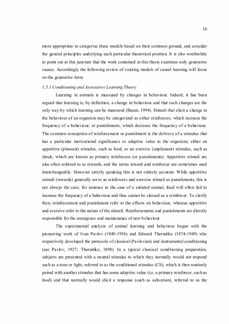
The experimental analysis of animal learning and behaviour began with the
pioneering work of Ivan Pavlov (1849-1936) and Edward Thorndike (1874-1949) who
respectively developed the protocols of classical (Pavlovian) and instrumental conditioning
(see Pavlov, 1927; Thorndike, 1898). In a typical classical conditioning preparation,
subjects are presented with a neutral stimulus to which they normally would not respond
such as a tone or light, referred to as the conditioned stimulus (CS), which is then routinely
paired with another stimulus that has some adaptive value (i.e. a primary reinforcer, such as
food) and that normally would elicit a response (such as salivation), referred to as the
Page 21
11
unconditioned stimulus (US). As conditioning progresses, a new pattern of behaviour is
seen to emerge such that the animal responds to the CS before the US is presented or even
if the CS is presented in isolation. This is known as the conditioned response (CR) and
tends to be similar in nature (though not always identical) to the unconditioned response
(UR) that would normally be elicited by the US. Pavlov’s dogs, for instance, after
repeatedly hearing a bell ring prior to being fed, developed a salivatory response to the
sound of the bell. The presentation of the CS and subsequent delivery of the US in classical
conditioning are arranged by the experimenter and thus not dependent on the animal’s
behaviour. In an instrumental conditioning protocol meanwhile, a response is required from
the animal before the satisfying outcome is obtained. In a typical experiment, Thorndike
placed a cat inside a puzzle box, from which it could escape by triggering the appropriate
mechanism. Thorndike noted that the time taken for the cat to escape decreased over
successive trials, and thus concluded that the animal learned to perform the correct response
to evoke the desired consequence of escape. The consequence thus reinforces the response.
Conditioning is thus an example of associative learning. The animal associates the
CS with the US in classical conditioning, and the response with the reinforcer in
instrumental conditioning. Through associative learning, stimuli that would not themselves
directly evoke an unconditioned response may acquire a motivational function and thus
serve as secondary reinforcers. Virtually any stimulus has the potential to provide
secondary reinforcement, with money an obvious example in human society. Money in fact
serves as a generalized secondary reinforcer through association with many primary
reinforcers (since it can be exchanged for food, water, shelter, and even sex) which is why
it can exert such powerful effects on behaviour. Associative learning is one of the most
fundamental forms of learning and is ubiquitous in the behaviour of organisms, from
humans to slime mould (Latty & Beekman, 2009). The parallels between associative
learning and causal learning should be immediately apparent, and causal learning is indeed
susceptible to many of the same influences as associative learning (Shanks & Dickinson,
1987), as shall now be further discussed.
1.5.1.1 The Rescorla-Wagner Model
Probably the most influential model of learning ever developed is the associative
model of Rescorla and Wagner (1972) which at time of writing has been cited in over 3500
Page 22
12
scholarly articles. The Rescorla-Wagner model (RWM) has enjoyed such tremendous
success due to its simplicity, elegance, and moreover due to its ability to account for
various phenomena of conditioning such as blocking (Kamin, 1969). The model was
developed specifically as an account of Pavlovian conditioning, and specifies the change in
associative strength between CS and US on a given conditioning trial according to the
following equation:
∆V = αβ(λ – ΣV)
where ∆V is the change in associative strength, α is the salience of the CS, β is the learning
rate parameter for the US, λ is the current magnitude of the US, and ΣV is the current level
of association between the CS and US (summed over previous trials) for each CS present
on the current trial. More simply, we may term λ as the actual outcome and ΣV the
expected outcome. The RWM is thus a trial-based error-correction model where the animal
learns through surprise, in other words through the discrepancy between what is expected to
happen and what actually happens.
A trial on which the US follows the CS serves to increase associative strength
between them, with successive CS-US pairing resulting in (increasingly smaller)
increments in associative strength until the maximum level of association is reached, and
learning has reached asymptote. If the US is absent on a given trial, then λ is 0 and there
will be no increment in associative strength. Indeed if some conditioning has already taken
place, ΣV will be positive and ∆V will hence be negative, producing a decrement in
associative strength. Nonreinforcement thus weakens an existing association. Associative
learning then, as specified by the RWM, is sensitive to the statistical relation or
contingency between CS and US just as the contingency between cause and effect shapes
causal inference.
One of the most notable successes of the RWM was its ability to account for cue
competition. This phenomenon was first observed by Kamin (1969) who demonstrated a
“blocking” effect in aversive conditioning with rats. In what is now the standard blocking
paradigm, the subject initially received CS1 � US in an initial training phase before
undergoing subsequent training with a compound stimulus CS1CS2 � US (in Kamin’s
experiments, the US was a shock, CS1 a light, and CS2 a tone). At test, subjects exhibited a
reduced CR to CS2 compared to control animals that did not experience the initial training
Page 23
13
with CS1 alone. Learning the CS1 � US association thus appeared to block learning about
CS2, providing clear evidence of competition for associative strength between cues.
Blocking is easily explained by the RWM. Since by the end of phase 1, the US is perfectly
predicted by CS1, there is no discrepancy between the expectation and outcome. In phase 2
then where CS2 is presented, λ is equal to ΣV and hence ∆V is 0. CS2 thus fails to acquire
associative strength. Despite a clear predictive relationship between CS2 and the US in the
second training phase, CS2 is redundant as a predictor because CS1 has already been
established as a perfect predictor of the US. The blocking effect thus further emphasized
the sensitivity of conditioning to the statistical relationship between events.
1.5.1.2 The Role of Time from an Associative Perspective
In addition to the statistical relations between cues and outcomes, conditioning is
also highly sensitive to the temporal arrangement of events. Indeed, prior to the
development of models such as the RWM, contiguity was held to be the dominant principle
of learning in traditional associative theories (Gormezano & Kehoe, 1981), with the “Law
of Contiguity” stating that if two events occur simultaneously, then the reoccurrence of one
event will automatically evoke a memory of the other. In other words, contiguity was
considered to be both necessary and sufficient for the formation of an association. Though
this assertion has since been toned down in light of new evidence (as shall be discussed
further on), contiguity remains a central determinant for conditioning.
The importance of contiguity has been made evident through the comparison of
different conditioning protocols. In what is known as delay conditioning, the CS will first
be presented and the US then delivered either while the CS is still present (so CS and US
overlap) or else immediately following CS termination. The delay between CS and US
onset is referred to as the interstimulus interval (ISI). Meanwhile, there is an interval
separating CS termination and US onset, this is known as trace conditioning, as
conditioning is assumed to rely on a trace memory or representation of the CS, since it is no
longer present. The terminology can sometimes be confusing – in trace conditioning there
is a delay separating CS and US, while in delay conditioning the US paradoxically follows
the CS without delay. The “delay” in the term instead refers to that between CS and US
onset, and serves to distinguish from simultaneous conditioning where CS and US onset is
concurrent. It is well-established that (generally) trace conditioning is less effective than
Page 24
14
delay conditioning, and that long-delay conditioning less effective than short-delay
conditioning, with the CR taking longer to develop (Solomon & Groccia-Ellison, 1996;
Wolfe, 1921) and being diminished either in magnitude (Smith, 1968) or in rate (Sizemore
& Lattal, 1978; Williams, 1976). Indeed with longer trace intervals, conditioning can fail to
occur altogether (Gormezano, 1972; Logue, 1979), though this is highly dependent on the
nature of the stimuli entering in the relationship, as the following paragraph shall explain.
The influences of temporal contiguity can be incorporated into models of conditioning such
as the RWM by adjusting the value of parameters such as α and β .
Yet, just as with causal learning, there are exceptions to this contiguity principle.
The blocking effect, in addition to showing the sensitivity of conditioning to the statistical
relationship between events, demonstrated that contiguity alone was not sufficient for
conditioning to occur. Although a cue and an outcome may occur contiguously, an
association between the two will not be learned if the cue is redundant as a predictor.
Furthermore, there is evidence to suggest that a lack of contiguity is not necessarily a
barrier to associative learning. In studies by John Garcia and colleagues involving
conditioned taste aversion (now commonly dubbed the Garcia effect), rats were given a
gustatory stimulus (such as flavoured water) followed by the inducement of nausea
(through administration of x-rays, or substances such as lithium chloride or apomorphine
hydrochloride), and subsequently demonstrated avoidance reactions to the gustatory
stimulus. Importantly, this conditioned taste aversion was readily established even when the
onset of nausea is delayed by more than an hour after the gustatory stimulus (Garcia, Ervin,
& Koelling, 1966). In an extension of this work, Schafe, Sollars and Bernstein (1995) have
shown that rats fail to acquire conditioned taste aversions when the CS-US interval is very
brief. Such results indicate that not only is contiguity not always essential for conditioning,
but it can actually prevent conditioning in certain circumstances. These findings have been
explained by postulating an innate bias such that certain cues and consequences are more
readily associable, with these hard-wired preferences presumed to have arisen through
natural selection. Garcia and Koelling (1966) indeed demonstrated that particular outcomes
tend to become associated with particular stimuli, even when other stimuli are presented
concurrently and thus have equal predictive value. While rats in their experiments
associated internal malaise with gustatory stimuli, they associated external pain (e.g.
Page 25
15
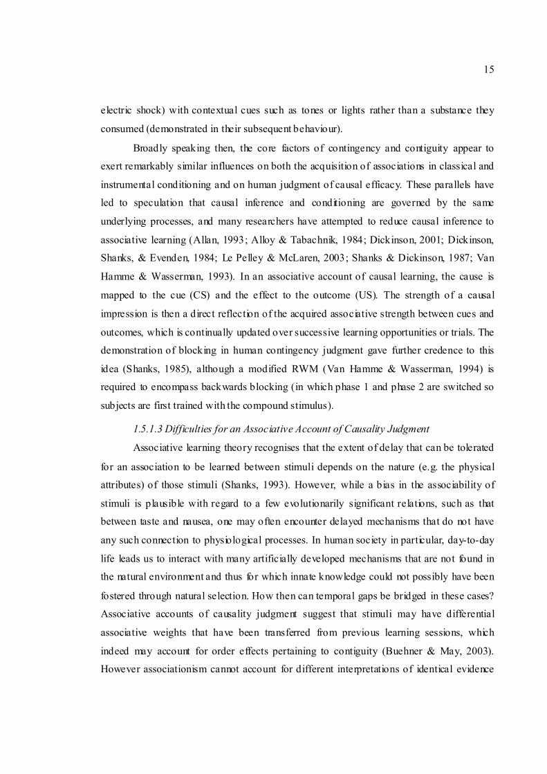
electric shock) with contextual cues such as tones or lights rather than a substance they
consumed (demonstrated in their subsequent behaviour).
Broadly speaking then, the core factors of contingency and contiguity appear to
exert remarkably similar influences on both the acquisition of associations in classical and
instrumental conditioning and on human judgment of causal efficacy. These parallels have
led to speculation that causal inference and conditioning are governed by the same
underlying processes, and many researchers have attempted to reduce causal inference to
associative learning (Allan, 1993; Alloy & Tabachnik, 1984; Dickinson, 2001; Dickinson,
Shanks, & Evenden, 1984; Le Pelley & McLaren, 2003; Shanks & Dickinson, 1987; Van
Hamme & Wasserman, 1993). In an associative account of causal learning, the cause is
mapped to the cue (CS) and the effect to the outcome (US). The strength of a causal
impression is then a direct reflection of the acquired associative strength between cues and
outcomes, which is continually updated over successive learning opportunities or trials. The
demonstration of blocking in human contingency judgment gave further credence to this
idea (Shanks, 1985), although a modified RWM (Van Hamme & Wasserman, 1994) is
required to encompass backwards blocking (in which phase 1 and phase 2 are switched so
subjects are first trained with the compound stimulus).
1.5.1.3 Difficulties for an Associative Account of Causality Judgment
Associative learning theory recognises that the extent of delay that can be tolerated
for an association to be learned between stimuli depends on the nature (e.g. the physical
attributes) of those stimuli (Shanks, 1993). However, while a bias in the associability of
stimuli is plausible with regard to a few evolutionarily significant relations, such as that
between taste and nausea, one may often encounter delayed mechanisms that do not have
any such connection to physiological processes. In human society in particular, day-to-day
life leads us to interact with many artificially developed mechanisms that are not found in
the natural environment and thus for which innate knowledge could not possibly have been
fostered through natural selection. How then can temporal gaps be bridged in these cases?
Associative accounts of causality judgment suggest that stimuli may have differential
associative weights that have been transferred from previous learning sessions, which
indeed may account for order effects pertaining to contiguity (Buehner & May, 2003).
However associationism cannot account for different interpretations of identical evidence
Page 26
16
achieved through abstract concepts, such as implicit manipulation of timeframe assumption
(Buehner & May, 2002). Thus, it is appropriate to consider other theories which
acknowledge other means whereby the connection between a candidate cause and a
temporally distant effect may be bridged.
1.5.2 Causal Mechanism and Power Theories
A significant aspect of traditional associative theories is that they inherited Hume’s
empiricism; they are data-driven or “bottom-up” in the sense that only the observable
properties of stimuli such as contiguity are considered to contribute to learning. However, a
number of findings have proven problematic for this empiricist approach applied to causal
inference. People appear to have pre-existing conceptions both about the types of stimuli
that are able to elicit certain outcomes and the timeframes involved in such processes, and
can use this knowledge to guide causal inference (Buehner & May, 2002, 2004; Einhorn &
Hogarth, 1986). Purely bottom-up accounts do not allow the scope for influences such as
higher- level knowledge on learning and therefore struggle to explain such effects where
there is no plausible prior associability bias. Alternatives to the empiricist approach
therefore embrace instead the philosophical position of Immanuel Kant (1781/1965), who
proposed that people have intuitive ideas about causality that provide a framework for
learning new relations. That is, causal relations need not be derived solely from empirical
observation; inference may also be facilitated or constrained by top-down information.
Causal mechanism or power theories of causal learning stem from the Kantian
rather than the Humean perspective. The central underlying principle of this view is that
successful causal inference hinges upon belief in or knowledge of a causal mechanism – a
specific process connecting causes to their effects and thus creating an intuition of necessity
between the two (Ahn, Kalish, Medin, & Gelman, 1995; White, 1989). According to this
view, causes are not just passively followed by effects, but rather actively generate their
effects by exerting their causal power. This may be seen as the transmission of force,
energy or some other property from one element to another (Peter A. White, 2009). This
position is motivated by the same cautionary mantra that is drummed into any aspiring
scientist or statistician; that correlation or covariation does not necessarily imply causation.
The key contribution then of mechanistic knowledge is in making the mental leap from an
observed covariation to the inference of a causal relation. It is therefore considered that
Page 27
17
people do not infer causality unless they know of a plausible mechanism by which these
events could be linked. Such a perspective has however been criticised as being hamstrung
by circularity: If top-down assumptions about mechanism govern causal inference, where
do such assumptions come from in the first place?
1.5.2.1 The Power PC Theory
Cheng (1997) attempted to synthesize the ideas of Hume and Kant, and refine the
causal power account, by proposing that empirically observable data (in the form of
contingency information) serves as the initial input for causal learning, while prior
knowledge then guides inferences drawn from this data. The prior causal knowledge
assumed here is general rather than specific. That is, mechanistic knowledge that is initially
acquired from empirical observations can then subsequently then be generalized to novel
learning situations (see Liljeholm & Cheng, 2007), hence overcoming the problem of
circularity.
According to Cheng (1997), observed deviations in human causal judgments from
measures such as ∆P are due to fundamental assumptions that people make about the nature
of causality that go beyond mere covariation, such the assumption of causal power. Such
deviations in judgement include sensitivity to changes in the base rate of the effect, P(e|¬c),
when ∆P is constant. To address these shortcomings of ∆P, Cheng advanced the power
theory of the probabilistic contrast model, usually shortened to PowerPC. This approach
focuses on the generative (or inhibitory) power of the cause, that is, its capacity to produce
(or prevent) the effect independently of all other potential causes. Causal power is
computed as:
∆P / 1 – P(e|¬c) for generative causes
–∆P / P(e|¬c) for preventative causes
Causal power is thus further distinguished from covariation models by making different
predictions from identical contingency data depending on whether the cause is assumed to
be generative or preventive, providing greater flexibility. One well-documented phenomena
of causal induction that covariation models cannot account for but that is predicted by
Power PC is the problem of ceiling effects. For example suppose one wished to test
whether a new type of medication produced nausea as a side effect. If every participant
experienced nausea after taking the medication, P(e|c) = 1 and the scientist might conclude
Page 28
18
that the medication was a very strong cause of nausea. But suppose every participant was
feeling nauseous to begin with; the results would then be uninterpretable; the participant
might well have developed nausea after taking the medication but since they were already
feeling nauseous this cannot be evaluated. ∆P in this case would be zero; P(e|c) – P(e|¬c) =
1 – 1 = 0, therefore predicting that the medication would be judged as noncausal. In
contrast the Power PC model, taking the generative form of the equation, would not return
a value in such a case, as the equation attempts to divide by zero. Power PC thus correctly
predicts that humans in such a situation would refrain from making a causal judgment
rather than concluding that the medication does not cause nausea.
In similar fashion, consider again the above clinical trials scenario but instead
assume that the medication was supposed to prevent (or relieve) nausea. Since none of the
participants experienced relief, one can, in this case, rationally conclude that the medication
was ineffective as a preventive cause of nausea. The predictions of causal power and ∆P
here then are equivalent for the preventive case but differ in the generative case when P(e|c)
= P(e|¬c) = 1. Meanwhile, if the base rate was zero and once again P(e |c) = P(e|¬c), causal
power predicts that humans will be unable to make a causal inference in the preventive case
(as there is no opportunity for the cause to exert its effect) but will accord with ∆P in the
generative case.
Predictions of the PowerPC model thus more closely mirror human judgments than
∆P and have proven resilient to challenges from other researchers (see Buehner et al.,
2003). However, although PowerPC emphasizes the distinction between causation and
covariation, causal power is still computed using covariation information – indeed, the ∆P
statistic itself forms part of the Power PC model. The causal power perspective therefore
makes the assumption that an observed configuration of causes and effects can be
unambiguously interpreted to populate the cells of the contingency table. However, this is
not necessarily a given. Furthermore, the model does not explicitly represent temporal
information.
1.5.2.2 The Role of Time from Covariation Perspectives
From the causal power view and related perspectives, time is not bestowed with a
particularly privileged role in causal learning. Temporal information is instead used to
determine how events experienced in the input are assigned to the cells of the 2×2
Page 29
19
contingency matrix. Provided that this information can be discerned from the available
evidence, contiguity is not required to compute contingency. If there is temporal separation
between cause and effect, the assumptions regarding mechanism and the expectation of
timeframe determines how these events are interpreted. If a delay is anticipated, then the
effect will be attributed to the cause, and constituting a single case of cell A (c�e, or e|c),
as shown in Figure 1.2, strengthening the causal impression. If instead a contiguous
mechanism is expected, a delayed pairing will be interpreted as one case of cell B (c�¬e
or ¬e|c) and one case of cell C (¬c�e or e|¬c), weakening the causal impression. This is
known as the attribution shift hypothesis (Buehner, 2005). Contiguity is thus only a
necessity if a contiguous mechanism is expected; meanwhile longer delays can be tolerated
if a slower mechanism is hypothesized. Longer intervals however also increase the
likelihood of intervening events occurring between action and outcome, which compete for
explanatory strength and place greater demands on processing and memory resources.
Delays thus introduce added uncertainty as to whether a given effect was generated by the
cause in question or whether it was produced by some other mechanism. This can mean that
causal learning with delays may sometimes be problematic even when the anticipated
mechanism means delays are plausible.
Figure 1.2: The effect of attribution shift in parsing an event stream with a specific
timeframe assumed : c � e intervals that are longer than the temporal window
simultaneously decrease impressions of P(e|c) and P(¬e|¬c) while increasing impressions
of P(e|¬c) and P(¬e|c).
The causal power and mechanism theories thus reflect the view that learners adopt a
more active approach to inferring causality. Rather than just passively processing
information, we seek to impose structure on data, using heuristics and prior knowledge to
constrain causal inference. Such mechanistic beliefs are key to avoiding learning spurious
Page 30
20
relations. We do not, for example, learn that the crowing of a rooster causes the sun to rise,
despite the fact that former event reliably signals the latter, since we know of no plausible
mechanism by which the rooster crowing could influence the rising of the sun. A key
strength of such approaches to causal learning is thus the flexibility to allow for top-down
influences such as prior knowledge to assist in the comprehension of empirical sensory
data. From this perspective then, causal learning is more than the mere sum of its parts.
1.5.3 Causal Models and Structure Theories
A third perspective on causal learning embraces a framework developed in statistics
and computer science – probabilistic graphical models (Glymour, 2001; Pearl, 2000;
Spirtes, Glymour, & Schienes, 1993). As the name suggests, this framework utilizes graphs
to model probabilistic relations in a simple yet effective manner, in which variables such as
causes and effects are denoted by nodes, and causal connections are indicated by arrows
linking these nodes. These models are also commonly referred to as causal Bayesian
networks (often shortened to Bayes nets), since their application utilises principles of
Bayesian probabilistic inference. Named after its original proponent Reverend Thomas
Bayes (1702–1761), Bayesian inference is a form of logical reasoning whereby the
probability of a hypothesis is assessed by specifying some prior probability which is then
updated in the light of new, relevant data.
Figure 1.3 shows a graphical model expressing the causal relation “X causes Y”.
This is a prototypical example of a directed acyclic graph (DAG); directed in the sense that
X and Y are connected by a directed arrow from X to Y, rather than by an undirected link;
and acyclic as there is no corresponding arrow directed from Y to X, and so a path cannot
be traced from one node back to itself. DAGs are the most popular means of expressing
causal relations in a graphical model, and the intuitive simplicity of these models makes
them a effective tool for representing complex causal networks.
Figure 1.3: Directed acyclic graph representing causal influence of X on Y.
Page 31
21
The fact that the causal arrow extends from X to Y with no symmetrical link from Y
to X reflects causal directionality, such that X causes Y but Y does not cause X. A crucial
component to causal understanding is that causes produce their effects and not vice versa,
such that an alteration to X will consequently produce an alteration in Y, but that an
alteration to made directly to Y itself will not produce an alteration in X. The representation
of directionality is one of a number of key advantages afforded by Bayes nets.
1.5.3.1 Causal Model Theory
Waldmann and Holyoak (1992, 1997) argued that principles such as directionality
cannot be captured by mere associations, and pinpointed this failure to specify causal
direction as a major shortcoming of associative theories of causal learning. Waldmann and
Holyoak instead advocated a causal model theory, according to which humans have a
strong tendency to learn directed links from causes to effects, rather than vice versa, in line
with how information is represented in a causal graphical model. Importantly, this remains
the case even when an effect is observed temporally prior to the cause – for example, when
one sees smoke before one sees the fire that produces it. In such a case, the smoke is still
correctly identified as an effect of a temporally precedent cause, the fire, even if the fire is
seen only subsequently, or remains unseen. In other words, humans construct causal models
that correspond to the veridical temporal order rather than the perceived temporal order.
Inferring the presence of fire from the observation of smoke is an example of
diagnostic inference. Waldmann and Holyoak (1992) drew special attention to the idea that
people appear able to reason both predictively, from causes to effects, or diagnostically,
from effects to causes. In a typical conditioning preparation, the order of stimulus
presentation mirrors the temporal order of a predictive causal model. Cues (input)
correspond to causes, and effects to outcomes (output). According to an associative account
of causal learning, the strength of a perceived causal relation is assumed to be a reflection
of the associative strength between cues and outcomes (Van Hamme, Kao, & Wasserman,
1993). However as Waldmann and Holyoak illustrate, in diagnostic inference the input-
output sequence is reversed with respect to the true causal model. In an associative account
of causal learning, effects would be assigned to the input layer and causes would be
assigned to the output layer, based on the order of observation in a diagnostic causal model.
Page 32
22
Meanwhile according to causal-model theory, the causal order is preserved and people
should reason from effects to causes.
This distinction between associative and causal model theory has important
implications regarding stimulus competition. As Kamin’s (1969) blocking effect
demonstrated, cues compete for associative strength in conditioning, and the success of the
RWM is in part due to its ability to elegantly explain blocking. Associative theory makes
the same predictions of cue competition regardless of whether cues represent causes or
effects. Causal model theory meanwhile argues in favour of competition between causes
rather than cues. To illustrate, consider a common-effect model, where two causes jointly
influence the same effect – as an example, where both rain and a water sprinkler are
potential causes of the ground being wet. Suppose one knows that it is raining, one would
then predict the ground to be wet. Subsequently finding out that the sprinkler had been
turned on would not affect this prediction; the ground would still be wet. The sprinkler then
is redundant as a predictor if we already know that it is raining and if rain has been
established as a reliable predictor. Cues thus compete for explanatory strength as causes in
predictive inference. Instead then, consider a common-cause model, where both the ground
being wet and people using umbrellas may be attributed to the common cause of rain.
Noticing that the ground is wet might lead us to infer that it has been raining. Here
however, noticing a second effect, that people are carrying umbrellas, would not weaken
our impression of the first link between the rain and the ground being wet. Thus there is no
competition between effects. In contrast, according to an associative model, here the effects
would constitute cues, and the presence of the first cue should block learning about the
second. Using the blocking paradigm, Waldmann and Holyoak (1992, 1997) demonstrated
that human subjects indeed made judgments consistent with causal model theory rather than
associative theory (see also (Booth & Buehner, 2007; Waldmann, 1996, 2000).
The above examples depend on prior knowledge of the causal models in questions.
Causal model theory then argues in favour of an integrative process utilizing both empirical
data and existing knowledge, rather than a purely associative mechanism. In this regard,
causal model theory is remarkably similar to the causal power approach advocated by
Cheng (1997), described in the previous section. The defining characteristic of model-based
theories is instead their basis on the Bayes nets framework. Causal model theory initially
Page 33
23
focused on how people use causal models in reasoning and how different assumptions
about causal structure may lead to different predictions from identical data sets. Waldmann
and colleagues did not however attempt to specify how causal models may be used to
provide a computational account of how empirical data such as contingency and contiguity
combines in causal inference.
1.5.3.2 Bayesian Structure Learning
This challenge was taken up by Tenenbaum and Griffiths (2001, 2003; Griffiths &
Tenenbaum, 2005) who pointed out the inadequacy of existing normative models such as
∆P and causal power to account for various aspects of causal induction (including effects of
sample size and non-monotonic effects of base rate on judgments). They instead proposed a
Bayesian “causal support” model to address these shortcomings. At the heart of this
framework is the notion that causal induction involves two kinds of learning, identifying
causal structure and assessing causal strength. In other words, deciding whether there exists
a causal relationship (structure), and if so, the extent of any such relationship (strength).
Structure learning is the task of identifying the causal model and its functional form,
as may be represented by a causal graphical model. Prior knowledge of how the world
works is used to generate a “hypothesis space” of plausible causal models that could
account for observed sequences of events (Tenenbaum & Griffiths, 2003). The simplest
case of causal induction is learning the relationship between a single candidate cause and a
single effect, where values of cause and effect are constrained such that both may be either
present or absent on a given occasion (and the relationship may thus be represented in the
contingency matrix). Griffiths and Tenenbaum (2005) termed this as elemental causal
induction, a moniker that shall be adopted here henceforth. Structure learning in elemental
causal induction then is essentially a binary decision between two hypotheses, as shown in
Figure 1.4: h0, in which there is no causal relation between cause c and effect e, and e
instead occurs solely due to the influence of random background processes b; and h1, where
c has the generative power to produce e (and b still also produces e).
The strength of a causal relation may be denoted in a causal graphical model by the
use of parameters, such as w0 and w1 in Figure 1.4, where b produces e with probability w0
and c produces e with probability w1. Griffiths and Tenenbaum (2005) argue that both
causal power and ∆P are estimates of the parameter w1 and so are measures of causal
Page 34
24
strength. The graph h1 (that a relationship exists between c and e) is therefore assumed in
both models. The different predictions of the two models results from different
parameterization of the graph. Causal power (for generative causes) corresponds to a noisy-
OR parameterization, where parameters have independent opportunities to produce the
effect. ∆P meanwhile corresponds to a linear parameterization, where the parameters
interact (see Pearl, 1988, for further details).
Figure 1.4: Directed acyclic graphs representing the two basic hypotheses that are
compared in elemental causal induction.
1.5.3.3 Causal Support
Griffiths and Tenenbaum (2005) argue that the primary goal of causal inference is
the more fundamental task of recovering causal structure, as it must be determined whether
a causal relationships exists before the strength of any such relationship can be assessed. In
Bayesian structure learning, plausible causal structures within a hypothesis space are
evaluated in terms of the probability of obtaining the current data set given that structure,
P(D|hi). This value can be calculated by integrating over parameter values (see Griffiths &
Tenenbaum, 2005, and Cooper & Herkowitz, 1992, for computational details). In elemental
causal induction, there are only two causal models in the hypothesis space, h0 and h1.
Structural inference in elemental causal induction is then made by assessing the likelihood
of obtaining the observed data under each of these two hypotheses, formalized as a decision
using Bayes’ rule:
Page 35
25
Causal support is thus a measure of the extent to which h1 provides a better account of the
given data than h0. According to Griffiths and Tenenbaum, causal support may be likened
to a significance test of a hypothesis for which causal power is the effect size measure.
Griffiths and Tenenbaum (2005) went on to present five experiments demonstrating
the superiority of causal support over ∆P and causal power in terms of providing a better fit
with human judgments of causality across a number of different learning situations.
However, causal support is at its heart a probability based model, and Griffiths and
Tenenbaum acknowledge that it does not specifically address the dynamics of elemental
causal learning in continuous time. Although causal support does a tremendous job of
accounting for how human causal judgments are obtained from contingency information,
such information is not always clearly defined. Assigning combinations of events to the
cells of the contingency matrix is a non-trivial task, particularly when delays are involved,
but causal support does not provide a computational account of the effects of contiguity.
1.5.3.4 A Bayesian Perspective on Contiguity
In an updated computational framework entitled theory-based causal induction,
Griffiths and Tenenbaum (2009) advocate two central concepts. Firstly, that people
approach the problem of causal induction with prior knowledge, in the form of abstract
causal theories, that enable the generation of hypothetical causal models for a given
situation. The principle of Bayesian statistical inference is then used to select the best
model. Secondly, the framework emphasizes the importance of coincidences, such as in
patterns of spatial and temporal contiguity. Griffiths and Tenenbaum (see also Griffiths,
2005) argue that humans are attuned to the detection of such coincidences. Since
coincidences are by definition those events that are improbable, or in other words unlikely
to happen due to chance, then coincidences provide support for a causal relationship.
Indeed, noticing conspicuous coincidences has often led to causal discovery throughout the
history of science.
Patterns of coincidence in time and space provide very strong evidence for a causal
relationship. We will all have experienced, from time to time, the illusion of causality that
strong contiguity will confer. For example, if we drop a glass on the floor and suddenly all
the lights go out, we briefly experience the impression of the former having caused the
latter, although of course we know that there is no mechanism by which this could have
Page 36
26
occurred and so dismiss this coincidence as spurious. Experimental evidence of illusory
correlations produced by strong contiguity in the absence of supporting statistical
information has been provided in the literature (Bullock, Gelman, & Baillargeon, 1982;
Fiedler, 2000; Mendelson & Shultz, 1976). Of course, such apparent “coincidences” are
often not merely coincidental but in fact are the product of a genuine underlying
mechanistic causal connection.
Bayesian accounts are somewhat obscure with regard to the precise means by which
contiguity contributes to causal inference. Krynski (2006) attempted to outline how the
short delay advantage may be explained from a Bayesian perspective, by considering that
the temporal delays between cause and effect may be modelled as a probability density
function, characterized as a gamma distribution. The height of the distribution on the y-axis
for a given point on the x-axis corresponds to the likelihood of observing that particular
delay. Since short delays are inherently less variable than long delays, the peak of the
distribution is narrower and higher for short delays. Krynski then goes on to argue that a
rational approach to causal inference is to integrate over all possible delays, meaning that
the likelihood ratio is higher when the temporal intervals are shorter, thus providing more
evidential support for a causal relation. This account of the short delay advantage bears
striking functional similarities to an associative account, although obviously the two are
conceptually very different.
However, the Bayesian structural account does not necessarily predict a uniform
advantage for contiguity. Rather the timing of events may place constraints on the plausible
causal models in the hypothesis space. Certain temporal patterns are more characteristic of
certain causal models than others. In elemental causal induction, the temporal distribution
of events may either constitute evidence in favour of a causal mechanism or may indicate
that background processes are a more likely candidate for the observed temporal pattern.
Griffiths and Tenenbaum (2009) chose a very specific example to demonstrate the effect of
patterns of temporal coincidence, based on earlier work examining how people use
temporal information to infer hidden causes (Griffiths, Baraff, & Tenenbaum, 2004). The
experiment presented a fictitious scenario via a computer simulation involving a set of cans
arranged on a table, each containing an explosive compound called Nitro X. Participants
were informed that because of the instability of this compound, spontaneous combustion
Page 37
27
might produce an explosion of a can at any given moment, and further, that any exploding
can would propagate unseen shock waves which may in turn cause neighbouring cans to
explode in a chain reaction. The task required participants to decide whether a particular
temporal pattern of explosions was due to spontaneous combustion, explosion of a nearby
can producing a chain reaction, or some other unseen cause. Results indicated that when a
suitable time lag separated one can’s explosion from another, a causal chain was correctly
inferred. When several cans exploded simultaneously however, a hidden alternative cause
was assumed (such as a jolt to the table), thus demonstrating how temporal coincidences
influence model selection. Griffiths and Tenenbaum provided a fairly complex
computational account of these particular effects, but did not provide a more general- level
computational model for the effects of temporal distributions in causal induction.
Nevertheless, the Bayesian structure approach offers considerable advances in accounting
for and modelling the effects of contingency and contiguity in human causal learning.
1.5 Chapter Summary
Causal learning is a core cognitive capacity that enables us to understand, predict
and control our environment. Causal relations themselves are not directly perceptible by
our sensory systems, and thus they must be inferred from patterns of evidence in the
information that reaches us. Cues such as contingency and contiguity between putative
causes and effects tend to foster impressions of causality between those events.
Some theories of causal learning adopt the empirical view, that only observable data
may contribute to the induction of causal relations. An associative perspective purports that
causal learning is nothing more than the acquisition of associations between cues and
outcomes. Associations are continuously updated over successive learning instances, with
contingency and contiguity being determinants of the direction and size of changes in
associative strength. Problems for associative accounts of causal judgment include apparent
influences of prior knowledge in mitigating a lack of contiguity between stimuli, since such
theories cannot accommodate these top-down representations.
Causal mechanism and power views argue that human causal induction goes beyond
mere associations. Proponents of these perspectives argue that humans postulate specific
causal mechanism by which causes generate or prevent effects. This both constrains causal
Page 38
28
reasoning, such that spurious correlations where there is no plausible mechanism can be
ignored, and also enabling inference from statistical relations to be guided by top-down
knowledge. Such cognitive accounts provide the flexibility to account for phenomena such
as systematic variations in judgment of noncontingent relations (Cheng, 1997), effects of
prior experience (Buehner & May, 2003), and knowledge-mediation (Buehner & May,
2002, 2004; Einhorn & Hogarth, 1986).
Causal-model and structure-based theories meanwhile are inspired by the Bayes
nets graphical framework to model causal relations. Like the power view, structural
accounts endorse the idea that inference from empirical data is guided by top-down
influences in the form of abstract causal knowledge. Where these accounts differ is with
regard to structure versus strength. The Bayesian approach argues that causal power is an
attempt to estimate the strength of a c�e cause-effect relation, before having evaluated the
evidential support for the existence of this relation, and is thus to some extent putting the
cart before the horse. The Bayesian approach instead is concerned with identifying the
likelihoods of plausible causal models given the obtained data, ahead of attempting to
estimate the parameters of this model to evaluate causal strength. According to the
Bayesian approach, regularities and coincidences such as contingency and contiguity
constitute evidence in favour of a causal relation since such occurrences are unlikely to
happen due to chance.
The order in which these theories have been presented in this chapter largely
reflects their chronological development. Associative theory is the most longstanding while
the Bayesian computational (structural) account the most recent. As such, the associative
view has been the most subject to criticism, while more recent accounts have the benefit of
hindsight. The question of how people infer causal relations, despite great strides forward
in understanding of learning processes, remains both unresolved and actively debated.
Associative theorists have attempted to undermine each significant challenge to
associationism, including Power PC (Lober & Shanks, 2000), causal model theory (Shanks
& Lopez, 1996), and knowledge mediation (Allan, Tangen, Wood, & Shah, 2003), which in
turn has drawn ripostes from the original proponents of these accounts. Discussions range
from specific boundary cases and technical details, to the more fundamental question of
whether causal learning is an insightful reasoning process or simply the product of
Page 39
29
associations. Suffice it to say then that no model has yet offered a full and undisputed
account of human causal judgement. Any empirical study of the phenomena of causal
induction would thus do well to remain mindful of all perspectives, their relative merits and
predictions, and consider how well the various accounts correspond to actual human
judgment within the domain of interest. This thesis shall adopt this consideration and the
experiments which follow will consider both the predictions of associative and cognitive
perspectives and how well the obtained results accord with each perspective.
This introductory chapter has hopefully provided sufficient background on the
already recognised cues to causality and how each of these cues is considered to contribute
to causal learning from three distinct schools of thought on the subject. The following
chapter shall now introduce the concept of temporal predictability, which is the phenomena
of central interest to this thesis. This concept will be considered from a theoretical point of
view, in relation to the three broad perspectives identified in this chapter, before an
empirical investigation of this concept in the two subsequent chapters.
Page 40
30
Chapter 2 – The Potential Role of Temporal Predictability in Causal Learning
2.1 Introducing Temporal Predictability
Griffiths and Tenenbaum (2009) point to the discovery of Halley’s comet as a
striking example of causal induction through the use of knowledge and theories. Sir
Edmund Halley (1656-1742) noted that comets observed in 1531, 1607, and 1682 had all
taken remarkably similar paths across the sky. Halley’s friend and colleague Sir Isaac
Newton (1643-1727) had already outlined in the Principia Mathematica that comets tend to
follow orbits corresponding to conic sections. Using the principles of Newtonian physics,
Halley inferred that the three comets previously observed were in fact one and the same
comet following a regular solar orbit. As Griffiths and Tenenbaum suggest, Halley’s prior
knowledge of such physical theories was doubtless crucial to this successful calculation.
Perhaps the most potent clue to this discovery however was that the three comets had been
observed approximately 76 years apart from one another in each case. In other words, there
was a consistent temporal interval between the appearance of all three comets, that varied
(in relative terms) minimally. Such periodicity is congruent with a celestial body following
a regular orbit, and hence provided a strong indication that the three comets were in fact
one and the same. It was this periodicity that allowed Halley to predict that the comet
would return again in 1758 and indeed this prediction proved to be accurate, with Halley’s
comet visiting the Earth every 76 years since. This facility of consistent timing, to enable
predictions regarding the occurrence of future of events and specifically when those events
will occur, makes “temporal predictability” an apt term to describe such a feature.
As a more commonplace example, consider the following anecdote:
Dave, Jon and Tom are discussing their morning drives to work. Dave and Jon suffer a
similar problem in which they encounter sets of traffic lights that sometimes take a very
long time to change, even when no cars are coming through on the opposite side. Tom
suggests that they try flashing their headlamps at the traffic lights to induce them to
change, as he has heard a rumour that they are programmed to respond to the flashing
lights of emergency service vehicles. Both take his advice. Dave notices that every time he
flashes his headlamps, the traffic lights do in fact change after a consistent delay of around
Page 41
31
10 seconds. Jon tries it at the set of lights on his route; sometimes the lights change very
quickly, sometimes they take much longer, with little discernible pattern. Jon concludes the
lights are operating on a fixed program and his headlamps are not influencing them. Dave
instead decides that his actions are effective and continues to flash his headlamps when
held up at the traffic lights.
The above story is an example of how event timing influences the way in which we
learn about causal relations. Here, contingency information is unhelpful; the traffic lights
will change eventually, the concern is instead with when they will change. In this example,
it is not the absolute delay between candidate cause and effect on each instance that
eventually determines the conclusions drawn by Dave and Jon. Rather, their decisions are
based on the variation in the timing of events across the set of instances over which they try
out Tom’s suggestion. What eventually convinces Dave of the efficacy of his actions is the
consistency of the temporal interval across multiple events.
The pairing of a particular candidate cause and effect tends to be experienced
repeatedly rather than as unique, one-off occurrences. Causal relations are, after all,
manifestations of invariant physical laws governing events in the environment (Sloman,
2005). Likewise when testing a hypothesized causal mechanism, we will normally make
multiple attempts, as in the example above. Obviously over multiple cause-effect instances,
we will experience multiple cause-effect intervals. These intervals may remain constant, or
may vary from one instance to the next. The variation of the interval separating cause and
effect is a consideration that has been overlooked with alarming frequency in the literature.
When there is a degree of constancy in the duration of intervals, then one may be
able to predict, just as Halley did in the earlier example, when a particular event will occur.
The degree of accuracy possible with such predictions will likely be a function of how
consistent the interval is over time. If the temporal interval is fixed and always takes the
same value, the relationship may be said to be maximally predictable. Conversely, if inter-
event intervals vary from case to case, then predicting future events becomes a much more
difficult, if not impossible, task. The greater the variability of the intervals, the more
unpredictable the relationship. Under the former scenario, one may develop particular
expectations regarding the timing of events, whereas for the latter there is uncertainty as to
when an outcome may occur. However, what influence this distinction may have, if any, in
Page 42
32
the detection or appraisal of causal relations, is yet to be fully explored. To begin with then,
this chapter shall review the scant existing evidence relevant to temporal predictability,
before considering how such a feature might be accommodated within models of learning.
2.2. The Temporal Predictability Hypothesis
The ability to predict the occurrence of future events is of course one of the central
advantages afforded by causal understanding. Causal impressions may thus be considered
as a direct reflection of the extent to which the cause is a predictor of the effect. This
importance of predictability for causal learning was emphasized by Young, Rogers and
Beckmann (2005). Young et al. noted that the dominant approach in the literature was to
conceive of and define predictability in terms of statistical regularity, that is, whether the
effect will follow the cause (e.g. Siegler & Liebert, 1974). They instead sought to expand
this perspective to encompass temporal regularity, positing that causal impressions are
based on not just whether an effect will occur but also when it will occur. In line with this
perspective they proposed a “predictability hypothesis” to account for the dual influences of
contingency and contiguity on causal learning, arguing that while contingency conveys
predictability in a statistical sense, contiguity conveys temporal predictability.
Young et al.’s (2005) contention was that delays make it more difficult to predict
when an outcome will occur, due to the inaccuracy in remembering the duration of a delay.
The longer the delay, the greater the inaccuracy (Gibbon, 1977). This temporal uncertainty
creates weaker causal impressions. Young et al. elaborated further by adding the caveat that
longer delays might sometimes be preferable if such a delay is expected (and thus
predictable) due to instruction, prior knowledge or experience. Causality then may be
attributed to temporally separated events provided that “earlier events are good predictors
of whether and when later events will occur” (p321). However, Young et al. stopped short
of pointing out what seems a logical extension of this argument; that in order for a delayed
mechanism to be predictable, it must be temporally consistent.
Young et al. (2005) did not directly contrast fixed and variable delays in their
experiments. Instead they investigated the effects of filling the delay interval with an
auditory stimulus, they suggested would enhance the temporal predictability of the
outcome. Using variations of Michotte’s (1946/1963) launching effect, participants were
Page 43
33
shown computer simulations of one ball colliding into another, and were then asked to
provide a rating of the extent to which they believed the first ball was the cause of the
second ball moving. In trials where launching lacked temporal contiguity, causal ratings
were markedly decreased, in line with Michotte’s original findings. However, the
introduction of the auditory stimulus bridging the temporal gap between impact and launch
was found to reduce the delay- induced decrease in causal judgments relative to where no
such stimulus was provided. Young et al. interpreted this finding as evidence in favour of
the predictability hypothesis; however these results are also readily explicable from an
associative perspective, in terms of the auditory stimulus signalling the outcome (Reed,
1992, 1999). Young et al. therefore did not address the potential impact of variation of
delays from case to case, and so did not conceive of temporal predictability in the same
sense as described in the anecdotes with which this chapter opened. Instead, they
considered temporal predictability to be provided by contiguity, since shorter delays are
inherently less variable, and attributed the detrimental effects of delays to a lack of
predictability.
The goal of this chapter is to broaden the conception of the role of temporal
information beyond mere contiguity, and to reconstruct the temporal predictability
hypothesis to encompass the impact of delay variability. Rather than just being a
consequence of contiguity, temporal predictability can be conceived as the consistency of
intervals over multiple cause-effect pairings. If the temporal interval between cause and
effect is held constant across repeated instances, then the timing of the event becomes
highly predictable, even if the actual interval between cause and effect is long. Holding the
temporal interval constant therefore constitutes another means by which predictability may
be enhanced, in addition to providing instructions, appealing to prior knowledge, or
presenting an external cue such as an auditory signal. According to this ‘updated’ version
of the temporal predictability hypothesis, a consistent timeframe linking cause and effect
means that the cause is a good predictor of when the effect will occur. While as Young et
al. (2005) suggest, a short delay is more temporally predictable than a long delay, a fixed
long delay is more predictable than a variable long delay. Consistent delays thus constitute
temporal predictability, which should enhance impressions of causality. Fixed intervals
should therefore be more conducive to causal inference than variable intervals.
Page 44
34
2.3 Previous Empirical Research on Predictability
To date, the contrast between fixed and variable intervals in human causal learning
has received remarkably little empirical attention. One exception is a landmark early study
on detecting response-outcome contingencies by Wasserman, Chatlosh & Neunaber (1983).
They studied causal learning in a free-operant paradigm, where a response made during any
given trial could increase or decrease the likelihood of a light to illuminate at the end of that
trial. Their third experiment contrasted predictable conditions employing trial lengths fixed
at a constant value of 3s, against unpredictable conditions where trial lengths could take a
value of 1, 3 or 5s. Although fixed and variable conditions did not differ significantly, there
was a general trend indicating that the variable conditions received uniformly, if
marginally, lower ratings than their fixed counterparts. The implication of this research is
therefore unclear, and a closer systematic examination of predictability is warranted.
Indeed, Wasserman et al. (p. 428) stated:
“Our failure to find significant effects attributable to these factors in no way means
that manipulation of the same variables over a broader range of values would also
fail to yield reliable results; indeed, we still believe that such work would disclose
discernible differences. Our research can thus be seen as a guide to others in their
search for potent influences on the perception of response-outcome relations.”
In a related study, Vallée-Tourangeau, Murphy & Baker (2005) investigated the
effect of outcome density on causal ratings. They implemented conditions where the
timeline was segmented into 1s ‘timebins’. If a participant responded, a reinforcement was
presented at the end of the timebin. Action-outcome interval was thus variable depending
on the point at which the participant responded. This was then contrasted with situations
where the action-outcome interval was instead held at a constant interval regardless of
when participants responded. Vallée-Tourangeau et al. found the same apparent trend of
fixed- interval conditions attracting slightly higher ratings, but again this difference was not
found to be statistically significant.
With a dearth of conclusive previous experimental work, there is a lack of clear
understanding and characterization of the role of predictability in causal learning. The
initial goal of the empirical work of this thesis is to address this omission in the literature.
Chapter 3 shall present a series of studies intended to determine whether predictability does
Page 45
35
in fact exert an influence on judgments, and the nature of that influence. Before progressing
with these studies however, it is worth casting a broader glance at findings from the
learning literature that might have some bearing upon this issue of predictability. The non-
significant trends in the studies described above suggests that, if anything, causal relations
with fixed temporal intervals may be seen as more robust than temporally variable
relations. However, there is a wealth of evidence from studies of reinforcement learning
with animals which suggests that the reverse may be true.
2.4 Animal Preference for Variable Reinforcement
Inspired by the earlier work of Pavlov and Thorndike, the research of B. F. Skinner
(1904-1990) focused on extending and refining the experimental analysis of behaviour (e.g.
Skinner, 1938). Thorndike’s earlier experiments were in the form of discrete trials, in the
sense that the animal performed a single response (pressing the escape mechanism) to a
given stimulus (being in the puzzle box), with a reduction in the time taken to perform the
response the measure of learning. Skinner instead developed an apparatus where the animal
could make multiple responses to given stimuli – the operant conditioning chamber,
popularly referred to as a Skinner box. A typical chamber includes a food dispenser and a
lever or mechanism of some kind that can be operated by the animal. Under appropriate
circumstances, pressing the lever can release a food pellet from the dispenser into the
animal’s food trough. The animal is able to freely explore the chamber and may press the
lever at any point; hence this was referred to by Skinner as the instrumental free-operant
procedure (FOP). This procedure has become so widely adopted that the term operant
conditioning is often used synonymously with instrumental conditioning (though strictly
speaking instrumental conditioning is a broader term also including discrete trials
procedures such as those of Thorndike). Indeed the earlier described paradigms of Shanks
et al. (1989) and Wasserman et al. (1983) are variants of this basic procedure.
A longstanding method for the exploration of how relations between responses and
outcomes govern behaviour is the use of reinforcement schedules (Skinner, 1969). In
operant conditioning, not every response is followed by a reinforcer; instead, certain
conditions must be satisfied before reinforcement delivery. Such schedules of
reinforcement specify the input that is required for a reward to be delivered. The two most
Page 46
36
common schedules used in behaviour analysis are ratio schedules, where a certain number
of responses are required before a reward is received, and interval schedules, where
reinforcement is provided following the first response after a given period of time has
elapsed. For example in a fixed-ratio (FR) 30 schedule, the reward is dispensed after every
30 responses, and in a fixed- interval (FI) 30 schedule, the reward is dispensed following the
first response after a 30 second period has elapsed (from the dispensation of the previous
reward). These schedules can also be variable as well as fixed; for instance on a variable-
interval (VI) 30 schedule, the amount of time after which a reward can be received varies
about an average of 30s, with the specific interval for any one trial falling within a pre-
defined range with 30s as the midpoint, for example 0-60s, 15-45s, or 20-40s.
Higher response rates on a particular schedule are generally taken as an indicator of
preference; in other words, that the animal has identified that there is a greater potential for
reward on that schedule. Naturally, a schedule providing a faster rate of reinforcement, or
requiring less input to receive a reward, will be preferred to a slower or more demanding
schedule. For instance, a FR10 schedule will be preferred over a FR100 schedule since the
latter requires ten times as much work for a given reinforcement. But certain types of
schedules are preferred over others even when the rate of reinforcement is the same. It is a
fairly well-established finding in the behaviour analysis literature that animals tend to
respond more frequently during variable-interval schedules compared to fixed-interval
schedules (Bateson & Kacelnik, 1995; Davison, 1969; Herrnstein, 1964; Killeen, 1968). It
has been argued that such findings are artefacts of the task; if one assumes that the animal
can learn the temporal intervals in a fixed preparation (cf. Gallistel & Gibbon, 2000a), then
it can restrict its responding to the point when it expects reinforcement to be delivered. If
instead intervals are variable then such a strategy will be ineffective; the best chance for
receipt of reward is to continue responding frequently throughout the schedule.
However, it has also been demonstrated that animals prefer variable over fixed
response-to-reinforcer delays when choosing between alternatives. For instance, Cicerone
(1976) employed a free-operant procedure in which pigeons were presented with two,
concurrently available, response keys. Variable-length delay intervals were superimposed
on the reinforcers scheduled with one response key while delay intervals of constant length
were superimposed on the reinforcers assigned to the other. The results showed that
Page 47
37
pigeons preferred variable over constant delays of reinforcement, responding more
frequently on the variable-delay key, and furthermore that this preference for variability
increased as the range of the interval lengths increased. Many other studies have also found
that organisms prefer aperiodic over periodic reinforcement delays (Bateson & Kacelnik,
1997; Mazur, 1984, 1986) thus indicating that this goes beyond task demands and reflects
an inherent property of variable reinforcement delay that makes it preferable.
While it is clear that performance on schedules of reinforcement and causal
inference in humans are not equivalent tasks, the preference for variable reinforcement
shown in non-human animals may be indicative of a general facilitatory effect of variability
in learning preparations. As Reed (1993) points out, while a relationship linking a response
to an outcome is not necessarily a reinforcement schedule, it is nevertheless possible that
“human perception of the causal efficacy of responses may be influenced by such schedules
of outcome presentation in some systematic manner” (p.328). A consistent preference for
variability may well be something that generalizes across learning domains.
Drawing inspiration from such studies of animal reinforcement to make forecasts
regarding temporal predictability is of course the same approach taken by many proponents
of associative accounts of causal learning, who have illuminated numerous ways in which
human causality judgments mirror simple conditioned behaviour. At this point then, it
seems appropriate to revisit the associative account, along with the other theoretical
perspectives on learning that were outlined in Chapter 1, and attempt to discern how
predictability might be accommodated in these theories. This will enable the results
obtained from these experiments to provide a contribution to the advancement of causal
learning theory as well as their empirical significance in their own right.
2.5 Theoretical Perspectives on Predictability
2.5.1 An Associative Analysis of Temporal Predictability
The dominant theory of animal behavioural processes is associative learning theory
(Mackintosh, 1983; Rescorla & Wagner, 1972). According to an associative account of
causal learning, causal relations are represented by the strength of an association between
putative causes and effects which is determined by the increment (or decrement) of
Page 48
38
associative strength over repeated learning trials. Effects are considered to be reinforcers to
the conditioned stimulus or response which is considered as the cause.
The impact of contiguity on causal learning is addressed by the supposition that the
greater the temporal separation between stimuli, the less associative strength that is
acquired as a consequence of their pairing (Shanks, 1987). In classical conditioning, this
could be due to the representation of the CS held in memory decaying over time (Wagner,
1981). Meanwhile in operant conditioning, the value of the reinforcer becomes diminished
as the delay until its receipt is increased, so a delayed reinforcer contributes less associative
strength compared to an immediate one.
It is important to note at this juncture that many distinct models of associative
learning have been proposed over several decades of research in this area. Although these
models may often be grouped together under the same umbrella term, there is no
unanimous agreement between different models on the role of time in learning. In the final
chapter of this thesis, I shall examine a number of specific associative accounts individually
and in more detail, to assess their compatibility with the results presented herein. Generally
speaking however, when associative learning is applied as an account of causal learning in
humans, the essential principles of traditional associative theories such as the Rescorla-
Wagner (1972) model (RWM), as described in Chapter 1, are applied. For the purpose of
outlining an associative account of temporal predictability then, these principles shall for
the moment be assumed.
Models of associative learning such as the RWM may be capable of representing
temporal information through the learning rate parameters such as α and β , which refer to
the salience of the CS and US. For instance, if it is assumed that the representation of the
CS held in memory decays over time, then the value of the α parameter will decline,
resulting in smaller increments in associative strength when delays are greater. Associative
accounts of the effect of contiguity, as exemplified by the RWM, thus assume a monotonic
influence of time in learning, such that longer delays result in weaker associations. The
overall extent of contiguity may thus serve as a potent determinant of the strength of
acquired associations. One might therefore be tempted to assume that whether contiguity is
fixed or variable should not matter, and the mean delay alone should determine the
contribution of contiguity. However, trial-based models such as the RWM update
Page 49
39
associative strength on a trial-by-trial basis, so each reinforcement makes an individual
contribution to the strength of an association. Any anticipated effect of predictability would
therefore depend on the rate at which associative strength changes with delay.
It is generally considered that the greater the extent to which the a stimulus appears
to reinforce behaviour, the stronger the acquired association. In other words, the amount of
conditioned responding that is exhibited, or the rate or magnitude of instrumental
responding (such as pressing a lever), is taken as an indication of the degree of association
between the CS and US (in classical conditioning) or response and reinforcer (instrumental
conditioning). Studies of delayed reinforcement in animals reveal that response rates
decline as a negatively-accelerated function of reinforcer delay (Chung, 1965; Williams,
1976). Taking response rate as a measure of associative strength then suggests that changes
in associative strength as a result of reinforcement diminish with delay of reinforcement
according to the same negatively accelerated function. If causal inference can be reduced to
associative learning, then it may be anticipated that delayed effects lose their capacity to
increase the cause-effect association in an analogous manner.
To then explain animal preference for variable- interval reinforcement, compare a
hypothetical set of fixed delays with a set of variable delays that have an equivalent mean
delay. Further assume that the fixed delay forms a central midpoint about which the
durations of the variable delays are evenly distributed. As an example, if the fixed delay
was 2s, then for every cause-effect pairing with a delay of 1s in the variable set, there
would be a corresponding pairing with a delay of 3s. Obviously an early outcome will
contribute more associative strength, and a late outcome less, relative to an outcome with a
delay intermediate between the two. Due to the negatively-accelerated form of the function,
associative strength is lost rapidly as contiguity first begins to decline, and less rapidly as
delays become progressively greater. The difference in associative strength between the
early (1s) and the intermediate (2s) outcome is greater than the difference in associative
strength between the intermediate (2s) and the late (3s) outcome. In other words, the loss in
associative strength by increasing delays from 1s to 2s is greater than the subsequent loss
by increasing delays from 2s to 3s. The combined associative strength of one early and one
late effect would thus be greater than that of two effects with a fixed intermediate delay,
despite the mean cause-effect delay being identical. In Figure 2.1, where ∆V is the change
Page 50
40
in associative strength, this could be expressed as: ∆Vx + ∆Vz > 2∆Vy. Consequently, it
would be expected that a series of effects with delays evenly distributed about a central
mean would accrue greater overall associative strength than where every effect follows the
cause after a fixed delay of a duration equal to that central point.
There has been some debate over the precise mathematical form of the function best
describing the decline in response rates with delay. For instance, Chung (1965) reported in
a signalled delayed reinforcement task that pigeons’ response frequencies declined
exponentially as a function of the delay interval. Other work (Herrnstein, 1970; Mazur,
1984) suggests that hyperbolic functions more accurately describe such trends. However,
for the above inequality to hold, the precise shape of the function is unimportant; any
negatively accelerated function would result in the same imbalance in accrued associative
strength. Under the assumption that causal learning is a direct reflection of associative
strength, it would then be anticipated that temporally-variable conditions would give a
stronger overall impression of causality than predictable conditions, and thus attract higher
causal ratings.
Figure 2.1: Potential differences in accrued associative strength between fixed-interval and
variable-interval conditions according to a hyperbola- like discounting function of delayed
events.
Page 51
41
However, this prediction might be considered as somewhat counter- intuitive. One
might be more inclined to expect predictability to provide confirmatory evidence for a
causal relationship, as was the case in the anecdotes at the opening of this chapter.
Consistency of the temporal interval separating candidate cause and effect could be taken
as symbolic of a genuine relationship between them, in much the same way as statistical co-
occurrence. If causes are hypothesized to bring about their effects by means of a particular
mechanism or sequence of events, it seems reasonable to suggest that (provided the
mechanism remains unaltered) there should be a degree of regularity in the timeframe over
which these events unfold. Let us therefore turn now to consider other theories of causal
learning which may generate predictions in accordance with this intuition.
2.5.2 The Attribution Shift Hypothesis
From a covariation perspective of causal learning, a potential explanation for the
effect of predictability is the attribution shift (Shanks & Dickinson, 1987). This has was
earlier outlined as an account for the detrimental effect of delay. Under this assumption, a
delayed action-outcome pairing is perceived not as a cause-effect pairing, c�e, but instead
as one instance of an action with no outcome, c�¬e and an outcome following no action,
¬c�e, as illustrated earlier in Figure 1.3. In terms of the 2×2 contingency matrix (Figure
1.2), this may be described as one instance of Cell B and one instance of cell C rather than
a single instance of Cell A.
However, this process is highly dependent on the size of the “temporal window”
that is adopted for event parsing. If a reasoner assumes a more relaxed timeframe over
which events may unfold, this enables temporally distal effects to be correctly attributed to
the candidate cause rather than disregarded as spurious. Previous work (Buehner, 2005) has
suggested that prior knowledge about existing causal mechanisms can lead to the
adjustment of this temporal window in this manner. In similar fashion, if the reasoner
repeatedly encounters evidence that is contradictory to their initial timeframe expectations,
they may revise their assumptions and adopt a new, more lenient temporal window. Thus if
the cause and effect are temporally separated, but this interval is constant, this may be
recognized over repeated instances and avoid the delayed effects being subjected to
attribution shift. Temporal predictability, therefore, may enable a learner to bridge temporal
gaps in causal induction through repeated exposure to the same temporal interval. In
Page 52
42
contrast, a variable interval might preclude recognition of the statistical regularity between
cause and effect, which in turn would mean that actual cause-effect pairings will be parsed
as instances of Cells B and C. The attribution shift hypothesis is therefore capable of
forecasting an advantage for predictability through the reduction of erroneous attribution of
delayed effects to random background processes. If the temporal assumptions are relaxed
and the window is expanded to encompass the c�e pairings, then with a fixed temporal
interval, all the pairings will be counted.
2.5.3 Bayesian Models
One final perspective takes a broader and more integrative viewpoint on the causal
learning process. The Bayesian structural approach (Glymour, 2001; Griffiths &
Tenenbaum, 2005, 2009; Spirtes et al., 1993; Waldmann & Holyoak, 1992, 1997) is
inspired by concepts from statistics and computer science, specifically, the use of causal
graphical models or Bayes nets to represent causal relations. Again, as with associative
learning, the Bayesian perspective is a general category of learning theories that
encompasses a number of individual models, which differ in their specificities but share
common principles.
Bayesian accounts of causal judgment combine both bottom-up empirical processes,
by which statistical inference from observable evidence forms the basis of causal induction,
with top-down modulation in the form of pre-existing causal theories. These abstract
theories serve to allow the generation of a hypothesis space of plausible causal structures
constrained by prior knowledge, experience and expectations. Under this framework, the
goal of causal induction is to first adjudge the best fitting causal model from the set of
possible structures, by evaluating the evidence in favour of a given structure. Once
structural inference has taken place, one may assess the strength of a causal relation
through parameter estimation. In elemental causal induction, structural inference is a binary
decision between two causal structures; either a causal relation exists (h1), or it does not
(h0). Among the leading accounts of causal learning in the Bayesian tradition is the causal
support model proposed by Griffiths and Tenenbaum (2005) which proposes that
judgments of causality are best described by a log ratio of the evidence for h1 compared to
h0, which reflects the degree of confidence that the causal relation c�e exists between a
candidate cause and an effect. Models such as ∆P and causal power meanwhile are
Page 53
43
considered to be estimates of the parameter w1 which specifies the strength of the c�e
connection. Bayesian perspectives thus emphasizes causal structure over causal strength.
Learning to impose structure on the world of sensation crucially depends on our
ability to identify patterns and consistencies in the environment which we can piece
together to produce a coherent picture. On a representational level, a Bayesian perspective
emphasises that such regularities or coincidences, whether statistical or temporal, are
evidence in favour of a stable causal mechanism. Both contingency and contiguity then
increase the evidence supporting h1 over h0. If it is assumed that a causal relation manifests
as a result of a specific mechanism, that this same mechanism is appealed to in each case,
and the processes involved in the mechanism unfold in a consistent manner, then it seems
reasonable to anticipate that this mechanism should have a consistent timeframe of action.
Constancy of temporal intervals is thus a further regularity in the environment that an
organism may be able to detect and use to construct an accurate representation of causality.
Meanwhile, spontaneous outcomes, generated by background processes rather than the
hypothesized mechanism, are assumed to occur according to a stochastic Poisson process,
where there is no reason to expect temporal consistency from one case to the next.
Although the likelihood of a spontaneous outcome increases with the time since the last
such outcome, since the probability of an outcome at each precise point is infinitesimal, the
likelihood of spontaneous outcomes repeatedly occurring following the same interval
would be a startling coincidence. Variability may thus be seen as indicative of a stochastic
process that b�e represents, while predictability is emblematic of the mechanistic process
c�e. From the Bayesian structure perspective then, temporal predictability would serve to
facilitate causal learning because temporal regularity between putative cause and effect is
much more likely if there exists a causal relation than if no such relation exists (and the
repeated regularity occurs by chance).
In computational terms, a Bayesian perspective is capable of predicting a
facilitatory effect of temporal predictability through likelihood distributions. Such
distributions reflect the likelihood of obtaining given data under a specific assumed
hypothesis. Recall from Chapter 1 the argument presented by Krynski (2006), mirroring
that of Young et al. (2005), that the short-delay advantage manifests because short delays
are inherently less variable. According to Krynski, this results in a narrow likelihood
Page 54
44
distribution with a high peak; in other words, the experience of shorter delays provides
strong confirmatory evidence for the existence of the hypothesized causal relation. In
contrast, longer delays (if the variance of such delays is proportional to the mean delay),
result in a wider likelihood distribution. By necessity, a wider distribution will also have a
lower peak, hence longer delays provide weaker confirmatory evidence for a causal
relation. If however the delay is fixed (or at least relatively consistent), then this would
result in a narrowing of the distribution, more closely converging on this fixed delay, with
the result that the peak of the distribution is elevated. In other words, making delays less
variable should have a comparable influence to shortening the delay Thus, the added
certainty provided by fixed delays would serve to increase the likelihood of the data under
the hypothesized mechanism, P(D|h1), and thus should enhance judgments of causality.
2.6 Chapter Summary
Temporal predictability refers to the constancy of a temporal interval between cause
and effect such that the time of occurrence of future effects of can be anticipated.
Predictability may be contrasted with interval variability where predicting the onset of an
effect becomes more difficult. Previous experiments (Wasserman et al., 1983; Vallée-
Tourangeau et al., 2005) have suggested that there may be the potential for differences in
the precise temporal arrangement of events in a learning preparation, such as with
predictability compared to variability, to elicit different responses or judgments of
causality. What is currently absent from the literature however is a systematic series of
studies specifically centred on elucidating the precise contribution of such temporal
arrangements to causal inference. The following chapter then attempts to definitively
address the potential role of temporal predictability in human causal learning. It will be
assessed whether case-by-case fluctuations in temporal delay can impact the causal
impression, or whether overall degree of stimulus contiguity across a learning preparation
is the sole contribution of temporal information.
Three broad theories of causal learning have been reviewed in attempt to discern the
predictions that they may generate regarding a potential role for temporal predictability.
From a traditional associative perspective, as exemplified by the RWM, the contiguous
pairings of cause and effect that are possible under a variable timeframe overcompensate
Page 55
45
for the smaller contribution of pairings with longer delays. Variability should therefore
confer an overall boost to impressions of causality compared to predictability (under the
assumption that delays are symmetrical about the mean). The predictions of this associative
account may appear counterintuitive, but are well- founded on a wealth of research from
reinforcement learning in animals. In contrast, cognitive perspectives allow for top-down
influences on learning, through which predictability could be taken as evidence of a
consistent underlying mechanism and thus facilitate causal inference. At a process level, a
covariation-based model may account for a predictability effect by postulating a relaxation
of the temporal window adopted for parsing the flow of input. A Bayesian account of
causal reasoning meanwhile appeals to the idea of delays being modelled as probability
distributions. According to this view, temporal predictability is highly unlikely to occur
under the causal model h0, where the effect in question is not a consequence of the
candidate cause, and regularity instead constitutes evidence in favour of a causal model h1
where the candidates are connected by a causal link.
The primary motivation underlying the experiments is to definitively address what
has surprisingly remained something of an oversight in the assessment of cause and effect
relations. However, since the outlined theoretical accounts make contrasting predictions, it
is evident that a manipulation of temporal predictability has the potential to provide
evidence that favours one account over another. Thus, results concerning predictability may
also confer some important theoretical insights and reinvigorate the debate between
associative and cognitive accounts of causal learning.
Page 56
46
Chapter 3 – The Role of Temporal Predictability in Instrumental Causal Learning
3.1 Overview and Introduction
This chapter comprises five experiments intended to investigate the role of temporal
predictability in human causal learning. The results constitute evidence in favour of a
facilitatory effect of temporal predictability. Discussion within this chapter focuses largely
on specific aspects of individual studies, as well as general methodological concerns.
Consideration of the wider theoretical implications of the results contained herein shall be
withheld until the General Discussion in Chapter 6, where they shall be discussed in light
of the theoretical perspectives outlined in Chapter 2, together with the results of the second
empirical section, Chapter 4.
It is evident that temporal predictability (or variability) has the potential to be added
as a fourth cue to causality (in addition to temporal order, contiguity, and contingency). A
number of perspectives on causal learning have been reviewed, all of which at least allow
for the possibility that temporal predictability may play a role in guiding causal
impressions. Given that existing empirical data is sparse and ambiguous, and that different
theoretical perspectives allow contrasting predictions, this chapter is dedicated to an
experimental analysis of the role of temporal predictability on causal inference.
The primary aim of this chapter is to determine whether predictability can influence
judgments by contrasting fixed and predictable temporal intervals with variable and
unpredictable temporal intervals. The results should inform as to whether predictability
enhances causal judgments, in line with a cognitive perspective and the temporal
predictability hypothesis, or whether instead variability is preferred, in line with a
reductionist approach and a simple associative account. It is also possible that no distinction
may be made between predictable and variable causal relations, with contingency and mean
overall contiguity remaining the defining principles. If however predictability can indeed be
identified as a cue to causality, the secondary aim of this chapter is to understand how
predictability might interact with the established cues of contingency and contiguity,
revealing whether they contribute independent or interactive influences.
For this initial foray into the investigation of temporal predictability in causal
learning, it was necessary to use a paradigm where the temporal interval between cause and
Page 57
47
effect could be tightly controlled, and in which candidate causes and effects were clearly
identifiable as such. Additionally it was considered prudent to avoid any unnecessary
complications or distractions by using a very simple and straightforward paradigm, such
that temporal distributions of events would be the most salient feature of the problem at
hand. The experiments conducted by Shanks, Pearson and Dickinson (1989) proved highly
effective in elucidating the role of temporal contiguity in human causal judgment. As a
computer-based adaptation of previous free-operant instrumental paradigms such as
Wasserman et al.’s (1983) earlier studies, this method allowed for the precise timing of
intervals to be specified and a wealth of behavioural data to be easily recorded. The
paradigm was used again with success by Reed (1992) and Buehner and May (2003). It was
therefore decided to base the initial experiments on a similar paradigm.
3.2 Experiment 1
This first experiment was modelled closely on Shanks et al.’s (1989) original study.
In each condition, participants were presented with a triangle on the screen and a button
labelled “PRESS” just beneath it. Participants were instructed that their task was to
investigate the extent to which their action (clicking on the button) could cause something
to happen on a computer screen (the triangle lighting up).
Participants engaged on a free-operant procedure (FOP) meaning that they were free
to choose whether and when to respond throughout the duration of the condition. Previous
studies have found scheduling of response-outcome contingencies on a FOP to be a highly
sensitive and unbiased method of investigating causal learning (Wasserman et al., 1983).
However in many such studies, the learning experience is segmented into pre-defined
‘response bins’ or learning trials (for example of 1-second duration). If a response is made
during this time bin, then it is reinforced at the end of the period. However, it is of course
possible that the participant may respond again during the time between a reinforced
response and the consequent outcome. This, and any further responses, would then go
unreinforced. Consequently, such a procedure fails when participants respond at a faster
rate than that corresponding to the pre-defined bin-size as only the first response within
each bin will have the potential to produce an outcome. This was pointed out by Buehner
and May (2003) who demonstrated that action-outcome delays in a standard FOP change
Page 58
48
P(e|c) and P(e|¬c), so that the actual contingency experienced by the participant is lower on
delayed than on immediate conditions. Furthermore, and of crucial importance for
scrutinizing the influence of temporal predictability, using this underlying trial structure
means that full control over the cause-effect interval cannot be maintained; while trial
length can be held constant, a participant may respond at any point during this trial hence
the interval between action and outcome may still vary. Wasserman et al.’s third
experiment should therefore more accurately be considered as a comparison of low-
variability against high-variability, rather than predictability against variability.
To avoid such problems, the experiments in this chapter did not employ pre-defined
learning trials or time-bins; instead, every response had the potential to generate an effect,
regardless of when it was made. The same response-outcome contingency as used by
Shanks et al. (1989) was employed again here: every press of the button had a 75% chance
of producing the outcome. If an outcome was scheduled, the effect occurred following the
programmed delay. The experimental program enabled the delay to be precisely specified
for every pairing of cause and effect, meaning it was possible to manipulate temporal
variability and delay across conditions while keeping constant the objective contingencies.
Of course, this trial- free instrumental procedure is not free from its own burdens, and one
may note that without defined trials there is inherent ambiguity with respect to matching
individual responses to individual outcomes. For instance, a participant could perform
several responses in quick succession and then observe a corresponding burst of effects
after the relevant delay. It would be difficult to match individual responses to specific
effects, and this would be amplified when the cause-effect interval is variable. Importantly,
however, by allowing each response to produce the effect (without limitations imposed by
trial structures) the overall objective contingency will remain unaffected by variations in
delay and variability of delay, which is essential to permit these factors to be assessed
independently. Whether the subjective impression of contingency (and indeed therefore in
this case also causality) remains unaltered by these manipulations is of course a different
question altogether, and in fact at the heart of the research reported here.
The experiment employed two mean delays, two and four seconds, and three
different types of temporal predictability. The first was a fixed, pre-determined delay that
remained constant throughout a given condition, and thus constituted maximal
Page 59
49
predictability. However, most natural causal relations rarely involve precise and perfectly
predictable cause-effect delays. Epidemiologists, for instance have long postulated that
disease outbreak follows infection after an incubation period described by a log-normal
distribution (Evans, 1993) centred around a mean expected wait time. Consequently, the
second level of temporal predictability sampled cause-effect intervals from a normally-
distributed probability density function, centred around a midpoint corresponding to one of
the fixed intervals (see Method below for more detail). Finally, as a maximally uncertain
control, a uniform random distribution was employed, where the delay could take any value
within a pre-defined range, with an equal probability of taking any particular value.
Importantly, these manipulations are distinct from Experiment 3 of Wasserman et al.
(1983); rather than restricting intervals to a small set of fixed values, I instead allowed
intervals to vary freely across a continuum.
Most real-world causal relations are assessed against a background of alternative
causes. For instance, whilst an illness may be the cause of a headache, a headache could
also potentially arise as a result of stress, tiredness, or dehydration. Identifying the crucial
relation from other spurious connections is a fundamental part of the induction process. In
order to preserve ecological validity in this respect, I also introduced three different levels
of background effects to the paradigm. This was done by scheduling the effect to occur a
pre-defined number of times, independently of the participant’s action, at random points in
time during the condition.
3.2.1 Method
3.2.1.1 Participants
31 undergraduate students with a median and modal age of 19 years were recruited
via an online participation panel hosted at Cardiff University. They received either £4
payment or partial course credit for participation.
3.2.1.2 Design
The experiment manipulated three factors – temporal distribution, background
effects, and delay. Temporal distribution had the levels fixed, normal, and random;
background effects had the levels zero, low, and high; delay had the levels 2 and 4 seconds.
Factorial combination of these levels resulted in a 3 × 3 × 2 within-subjects design,
producing 18 different conditions each of 90s duration.
Page 60
50
The probability of an outcome following an action, P(e|c), was .75 throughout all
conditions. Note that this probability was not defined relative to a particular unit of time;
instead, each button press had a 75% chance of causing the triangle to flash. If an event was
generated, the effect then occurred after the appropriate temporal interval had elapsed.
The three types of temporal distribution provided a manipulation of predictability
by controlling the variation of the temporal intervals in each condition. The interval for any
given action-outcome pairing was determined according to the particular combination of
delay and temporal distribution. In the fixed conditions, the temporal interval was always
the same, held at a constant value within the condition (i.e. 2 or 4 seconds). These values
then served as “midpoints” for the comparable normal and random conditions. For the
random conditions, the temporal interval for any given cause-effect pair was given by
generating a random value within the specified range. So for example in the ‘Random2’
condition, the interval could take any value between 0 and 4 seconds, with any value
equally as likely to occur as another. For the normal conditions, the delay was specified
according to a normal probability distribution with a range of 4 seconds, centred around the
midpoint. So for example in the ‘Normal4’ condition, interval lengths were drawn from a
normal distribution centred around 4 seconds, with minima and maxima of 2 and 6 seconds.
Accordingly values closer towards the midpoint of 4 seconds were more likely than values
towards the extreme boundaries of 2 and 6 seconds. Thus, the delay variance for normal
conditions should be smaller with respect to the random conditions.
In addition, three levels of non-contingent ‘background’ effects were employed,
where the outcome occurred independently of the response. As a baseline, I first applied a
zero rate of background effects – the effect did not occur in the absence of the cause and
P(e|¬c) = 0. In addition I created a medium rate, equivalent to 1 effect every 10 seconds,
and a high rate equivalent to 1 every 5 seconds. With a total condition time of 90s, this gave
9 and 18 background effects in total for the medium and high levels respectively, which
were distributed randomly throughout the condition.
Page 61
51
Figure 3.1: Diagram representing the three types of temporal distribution applied in
Experiment 1 at the two levels of mean delay.
Two questions were used as dependent measures to gauge participants’ impressions
of causal strength. One was based on a covariational understanding of causality couched
within a counterfactual question:
“Imagine you had pressed the button 100 times in this condition. How many of
these 100 presses would have caused the triangle to light up?”
The other was slightly more ambiguous and was aimed to appeal to the degree of perceived
control beyond pure covariation:
“Overall, to what extent do you feel pressing the button controlled the triangle
lighting up in this condition?”
Participants provided a rating between 0 and 100 for both questions.
3.2.1.3 Apparatus, Materials and Procedure
The experiment was programmed in Python 2.4 and conducted on Apple Macintosh
computers situated in individual testing booths. Participants used the mouse to click on the
“PRESS” button, and used the keyboard to type in their responses at the end of each
condition. After being welcomed by the experimenter and giving consent to participate,
participants read on-screen instructions which outlined the nature of the task.
Page 62
52
In each condition, a triangle was presented in the centre of the screen, along with a
button that participants were able to press, by clicking on it with the mouse. If a response
triggered an outcome, the triangle lit up for 250ms. Participants engaged in 18 different
free-operant procedures as described above, presented in a random order, with each
condition lasting 90 seconds. At the end of each, the screen cleared and participants were
asked to respond to the two questions described previously. Participants then typed in their
answers into the appropriate text box and clicked on the SUBMIT button to proceed to the
next condition. In total the experiment lasted around 35 minutes.
3.2.2 Results
3.2.2.1 Causal Judgments
Two different questions were posed at the end of each condition, intending to try
and capture fully all aspects of the participants’ causal impressions. The ‘contingency’
question is a well-established measure that has been used in many previous studies (Shanks
et al., 1989; Wasserman et al., 1983). The ‘control’ question meanwhile was rather more
ambiguous, which may propel participants to take temporal information into account in
providing their rating, and thus may provide a more useful measure for capturing any
influence of predictability. Accordingly it seems appropriate to focus initially on this latter
measure. Figure 3 shows mean ratings provided by participants for the ‘control’ question,
for all 18 conditions. For clarity, error bars are omitted; standard deviations can however be
found in Table 3.1. As expected, ratings were considerably higher in the shorter-delay
compared to the longer-delay conditions. Also in accordance with previous findings, ratings
declined as the rate of background effects increased. The effect of temporal predictability,
which is the factor of principal interest, is less immediately apparent. It can however be
seen that the fixed conditions consistently received higher causal ratings than their normal
and randomly distributed counterparts, while there appeared to be little difference between
the two distributed conditions.
A 3×2×3 within-subjects repeated-measures ANOVA corroborated these
impressions, finding significant main effects of temporal distribution, F(2,60) = 3.373,
MSE = 611.2, p < .05, ηp2 = .101; delay, F(1,30) = 20.91, MSE = 729.9, p < .0005, ηp
2 =
.411; and background effects F(2,60) = 27.49, MSE = 792.5, p < .0005, ηp2 = .478. Since it
was hypothesized that fixed interval conditions would draw higher ratings than their
Page 63
53
variable counterparts, Helmert contrasts, which compare each level of a categorical variable
to the mean of the subsequent levels, were performed to compare the fixed conditions with
the normal and random conditions combined. These planned comparisons confirmed that
fixed interval conditions (M = 52.70, SE = 1.933) received significantly higher ratings than
variable interval conditions (M = 46.95, SE = 1.269), F(1,30) = 4.984, MSE = 1235, p <
.05, ηp2 = .142, while in turn there was no significant difference between normal and
random conditions, F(1,30) = 0.050, MSE = 798.4, p = .825. None of the possible
interactions were significant.
20
30
40
50
60
70
80
none low high
Mean Control Rating
Background Effects
fixed 2s
normal 2s
random 2s
fixed 4s
normal 4s
random 4s
Figure 3.2: Mean Control Ratings for all conditions in Experiment 1 as a function of
background effects. Filled and unfilled symbols refer to mean delays of 2s and 4s
respectively. Delay variability is noted by different symbol and line styles. Error bars are
omitted for clarity.
Participants’ ratings for the ‘contingency’ question followed the a similar pattern as
for the ‘control’ question, with significant main effects for temporal distribution, F(2,60) =
3.851, MSE = 557.5, p < .05, ηp2 = .114, delay, F(1,30) = 20.84, MSE = 679.6, p < .0005,
ηp2 = .410, and background effects F(2,60) = 12.57, MSE = 556.6, p < .0005, ηp
2 = .295. Of
all the possible interactions, only that between delay and background effects was
Page 64
54
marginally significant, F(1,30) = 3.077, MSE = 523.6, p = 0.053, ηp2 = .093. Further
analysis of this interaction by examining simple main effects revealed a significant contrast
in the differences between zero and high levels of background effects at short and long
delays, F(1,30) = 5.007, MSE = 598.0, p < 0.05, ηp2 = .143, and a marginally significant
contrast in the differences between zero and medium levels of background effects at short
and long delays, F(1,30) = 4.062, MSE = 845.7, p = 0.053, ηp2 = .119. Using Figure 3.3 as a
reference, this would seem to indicate that broadly speaking, the influence of background
effects on contingency ratings was rather more muted at longer delays compared to short
delays. Aside from this interaction, participants apparently made little distinction between
the two dependent measures, with both eliciting similar responses. Indeed inspection of the
raw data revealed that they were treated as identical by considerable proportion of
participants, with scores matched in over a third of the total cases. It was therefore decided
to employ only a single dependent measure in subsequent experiments.
20
30
40
50
60
70
80
None Low High
Mean Contingency R
ating
Background Effects
Fixed 2s
Normal 2s
Random 2s
Fixed 4s
Normal 4s
Random 4s
Figure 3.3: Mean Contingency Ratings for all conditions in Experiment 1 as a function of
background effects. Filled and unfilled symbols refer to mean delays of 2s and 4s
respectively. Delay variability is noted by different symbol and line styles. Error bars are
omitted for clarity.
Page 65
55
3.2.2.2 Instrumental Behaviour and Outcome Patterns
Table 3.1 shows the behavioural data from the first experiment, for each of the 18
conditions. This includes response rate (i.e. mean presses per minute) within each
condition, and the corresponding rate of effects (outcome density). The experienced P(e|c)
is also shown, calculated as the proportion of responses that generated an effect (ignoring
background effects), for each participant in each condition. The mean interval between
cause and effect was likewise computed, and is shown with the standard deviation, as an
indication of temporal interval variance, in parentheses. In addition the mean ratings
provided for the contingency and control questions are also reported, again with standard
deviations in parentheses.
While the number of responses produced is fairly consistent across conditions, it
appears that conditions without background effects produced the highest response rates in
general, while the ‘Random4’ conditions (random distribution, 4 second delay) received
lower response rates. If for some reason different conditions are producing different
response rates in participants, then the effect of this manipulation may not be directly upon
causal rating but instead mediated through changes in response (and subsequent outcome)
density. It was thus necessary to verify whether the independent variables influenced
ratings indirectly by exerting an effect on behaviour. In addition, some fluctuations in the
actual delay and P(e|c) from the programmed values are also expected; while these were
assumed to eventually cancel out throughout the course of each condition (and certainly
across participants) it is possible that differences between conditions could remain and be
driving any observed differences in causal ratings.
To address these concerns, 3×2×3 within-subjects repeated-measures ANOVAs
were carried out on the data derived from participants’ instrumental behaviour. Due to a
small number of participants responding at a very high rate, the distribution of data for
response and outcome rate is positively skewed; hence response rates were normalized by
taking the square root. No significant effects of temporal distribution, F(2,60) = 0.456,
MSE = 1.536, p = .636, delay, F(1,30) = 0.003, MSE = 1.813, or background effects,
F(2,60) = 2.326, MSE = 1.633, were found on response rate. There was however a
significant distribution × delay interaction, F(1,30) = 3.578, MSE = 1.193, p < .05, ηp2 =
.123, specifically that for normal conditions, response rate was higher with shorter delays
Page 66
56
while for random conditions this pattern was reversed. However since this interaction did
not involve a systematic difference in overall response rates between fixed and variable
conditions, it is not problematic for the principal findings. Meanwhile, mean delay naturally
differed between different delay conditions, but was not significantly affected by either
temporal distribution or background effects (both ps > .3). Actual P(e|c) was also
unaffected by all three independent variables (all ps > .1). Participants’ causal judgments
were therefore not impacted by uncontrolled differences in instrumental behaviour or
deviations from programmed values.
Table 3.1: Behavioural Data for Experiment 1. Standard deviations are given in
parentheses.
Page 67
57
3.2.3 Discussion
The results of this experiment replicate well-established findings that a) in the
absence of delay expectations, cause-effect delays are detrimental to learning and b) adding
non-contingent background effects, thus reducing contingency by inflating the proportion
of e|¬c (cell C in Figure 1.2) likewise reduces causal ratings. This instils confidence in the
reliability of the paradigm. Of central interest, however, was the influence of temporal
predictability. The analyses confirmed that conditions with fixed temporal intervals
received the highest causal ratings, suggesting that enhancing predictability by holding the
cause-effect interval constant facilitated attribution, in line with predictions derived from
top-down theories of causal learning.
These effects of predictability do not appear to be obscured by non-contingent
background effects, as evidenced from a lack of an interaction between predictability and
level of background effects. This is perhaps surprising since if a non-contingent outcome
occurs between the cause and its generated effect, then a different (shorter) interval
between response and outcome will be experienced objectively, which should disrupt the
impression of predictability. However, since the free-operant procedure allows for
responses at any time, subjects are able to make several responses in succession, from
which a consistent delay may well become evident. Noncontingent effects that
subsequently intervene between the cause and a generated effect should then be correctly
attributed to background processes. One might then ask, if participants were able to connect
causes with their effects, why judgments were adversely affected by increasing background
effects. To address this question, it should be remembered that causal judgments tend not to
be solely based on P(e|c), but instead on normative measures of contingency that take the
base rate into account. The fact that the outcome occurs independently of the response will
thus reduce the contingency, even if contingent outcomes are correctly attributed to the
candidate cause (by inflating the value of cell C). The marginally significant interaction
between delay and background effects meanwhile is a finding that has not previously been
reported with any real emphasis in the literature. Specifically, this indicated that causal
ratings were less affected by the level at background effects when delays were long
compared to when delays were short, and only when contingency ratings were solicited.
This is potentially interesting and further research might wish to further explore whether
Page 68
58
this is a systematic effect or merely an anomaly. This result is however not in any way
problematic for the findings regarding predictability, and is largely irrelevant to the central
focus of interest, so will not be considered in more detail here.
While the fixed conditions clearly attracted the highest ratings, no distinction was
obtained between the normal (intermediate variability) and random (high variability)
conditions. Arguably, normally-distributed delays could have been expected to elicit higher
ratings than their uniformly-distributed random counterparts, due to the smaller variability
of delay in the former compared to the latter (as reported in Table 3.1). One possible
suggestion for this failure to find a significant difference is that the large number of
experimental conditions made it more difficult to distinguish one from another and thus
contributed to noise within the data. A more substantial explanation is that the normal and
random conditions were much more similar to each other than either was to the fixed
conditions. While the fixed conditions had no variability of delay, for the two distributed
conditions, there was a maximum range of four seconds within which the effect could occur
following a reinforced response, the only difference between these two being the likelihood
of the effect occurring at a particular point within this range. Rather than increasing or
decreasing the temporal range within which an effect could occur, I varied the probability
distribution according to which any given temporal interval was determined. Although the
variance of the delay was greater for random than normal conditions (Table 3.1), the
maximum range of interval variability was the same for each. It therefore seems an
appropriate next step to investigate the effect of modifying temporal predictability by
varying the size of the interval range. Will an increase in interval variability, and
concomitant unpredictability, lead to a corresponding decline in causal evaluations?
Experiments 2A and 2B sought to address this question.
3.3 Experiment 2A
Experiment 1 has demonstrated that maximally predictable conditions where the
temporal interval between cause and effect is fixed and constant elicit stronger judgments
of causality, relative to less predictable, variable conditions with the same average delay.
What has to be demonstrated clearly however is whether an increase in the variability of the
temporal intervals in a causal relationship produces a corresponding decrease in the
Page 69
59
evaluation of causal strength. As I already pointed out, the contrast of two differently
shaped distributions, where delays were distributed either normally or uniformly, but still
centred around the same mean, may not have produced sufficient differences in experience
to produce different impressions of causality. Experiment 2A thus sought to implement
differences in the degree of predictability by varying the range over which intervals could
vary, rather than the type of distribution from which they are drawn. If, as the results of
Experiment 1 suggest, predictability enhances causal judgments, then conditions with fixed
intervals should once again receive the highest ratings. Furthermore, if impressions of
causality decline as predictability is lost, then judgments should decline as the range of
temporal intervals increases.
A number of improvements were made to the paradigm. Firstly, only a single
question was deployed as a dependent measure of perceived causal effectiveness.
Experiment 1 found no systematic differences between the two measures used in that study,
so the focus on one question is economical both in terms of participant time and analysis.
Secondly, since Experiment 1 showed that the addition of random non-contingent outcomes
(while producing the expected main effect) had no interaction with either delay or
predictability, the independent factor of background effects was removed, thus reducing the
number of experimental conditions to six. Thirdly, I increased the time participants could
learn about each causal relation from 90 to 120s, comparable to earlier studies (Shanks et
al., 1989). Experiment 1 employed a shorter exposure time merely to prevent participant
fatigue when working though such a large number of conditions. Having streamlined the
number of conditions in this study, it seemed reasonable then to increase exposure time.
3.3.1 Method
3.3.1.1 Participants
42 undergraduate students from Cardiff University were recruited via an online
participation panel. Participants included both males and females, with a median and modal
age of 19 years. Course credit was awarded for participation. Due to an experimenter error,
one participant did not receive the correct materials and was dropped from the sample. One
further participant failed to comply with the instructions and was removed from the
analysis. 40 participants thus contributed data to the sample.
Page 70
60
3.3.1.2 Design
Two independent variables were manipulated – mean programmed delay and range of
temporal interval values. In similar fashion to the “random” conditions in Experiment 1, the
value of a temporal interval on any given cause-effect pairing could take any value within
the defined range, with uniform probability across the range. Interval range was thus a
manipulation of the level of temporal predictability – the wider the range of temporal
interval values, the greater the variation in the value that a temporal interval could take on
any one particular cause-effect instance, and thus the greater the variability of temporal
intervals throughout the experimental condition.
Delay had two levels, 3s and 6s. Range had three values: 0s, which meant that there
was no variation in the temporal intervals and the delay was fixed throughout the condition;
3s, which meant the temporal interval on a given cause-effect instance could take any value
within a range of 3s about the mean delay, or in other words 1.5s either side of this central
midpoint; and 6s, which meant temporal intervals could take any value within 3s either side
of the programmed mean delay. These were combined factorially to produce 6 different
conditions, each of which was experienced by every participant, producing a 2×3 within-
subjects design. As an example, in the 3s-range 3s-delay condition, cause-effect intervals
could take on any value between 1.5 and 4.5s. The six conditions are represented
diagrammatically in Figure 3.4.
Figure 3.4: Diagram illustrating the combination of the levels Delay and Range to produce
the six experimental conditions in Experiment 2A.
Page 71
61
3.3.1.3 Apparatus, materials & procedure
The experiment was run on an Apple “Mac Mini” running Windows XP and Python
2.4.1, with a 17” LCD display. The basic perceptual experience for participants was
virtually identical to that from Experiment 1, except that condition time was extended to
120s, and that I opted to use only a single dependent measure: “On a scale of 0-100, how
effective was pressing the button at causing the triangle to light up?” The experiment took
approximately 15 minutes to complete.
3.3.2 Results & Discussion
3.3.2.1 Causal Ratings
The mean causal ratings for Experiment 2A are shown in Figure 3.5. There is a
clear separation between delays of 3s and 6s, with the more contiguous conditions receiving
higher causal ratings. There also appears to be a general trend for predictability. While
there appears to have been no discernible influence of interval range for short-delay
conditions, with a longer mean delay causal ratings appear to decline in linear fashion as
temporal interval range is increased and predictability is reduced. This is suggestive of an
interaction between delay and predictability such that where inter-event delays are longer,
predictability becomes more important.
A 2×3 within-subjects ANOVA obtained the expected significant main effect of
delay F(1,39) = 19.57, p < .0005, MSE = 386.9, ηp2 = .334. However, contrary to my
predictions, there was no significant effect of interval range, F(2,78) = 1.759, p = .179,
MSE = 426.6, ηp2 = .043. Surprisingly given the trend in ratings in Figure 3.5, the
interaction between delay and range was also not significant, F(2,78) = 1.548, p = .219,
MSE = 472.6. The linear component of the main effect of predictability was however
marginally significant, F(1,39) = 4.005, p = .052, MSE = 374.7, ηp2 = .093.
Page 72
62
30
40
50
60
70
80
0s 3s 6s
Mean Causal Rating
Range of Temporal Intervals
3s
6s
mean delay:
Figure 3.5: Mean Causal Ratings from Experiment 2A as a function of temporal interval
range. Different symbol and line styles represent different delays. Error bars show standard
errors.
0s 3s 6s 0s 3s 6s
30.7 33.1 32.775 27.025 28.89744 27.575
20.2625 23.3 20.475
49.03
(25.85)
2983
(132)
3022
(272)
6000
(0)
0.746 0.750 0.747 0.761 0.772 0.748
mean
responses
mean
outcomes
actual P(e|c)
mean actual
delay
6075
(273)
67.15
(26.52)
65.95
(22.06)
66.93
(19.92)
61.05
(23.08)
56.25
(25.02)
delay
6s3s
mean causal
rating
23.05 24.7125 24.5625
3000
(0)
5989.5
(152)
range of temporal intervals
Table 3.2: Behavioural Data for Experiment 2A. Standard deviations are given in
parentheses.
Page 73
63
3.3.2.2 Behavioural Data
Table 3.2 summarizes the behavioural data for Experiment 2A. Once again to verify
that behavioural variance is not a confounding influence on causal ratings, the effect of the
independent variables on response rates was analyzed using a 2×3 within subjects ANOVA.
There was a marginally significant effect of delay on response rate, F(1,39) = 3.887, p =
.056, MSE = 876.1, ηp2 = .091, driven by slightly higher rates of responding in the short-
delay conditions. There was no significant effect of temporal interval range, F(2,78) =
1.066, p = .349, MSE = 690.8, and no significant delay × range interaction, F(2,78) = .186,
p = .831, MSE = 831.9. Response rates were therefore largely unaffected by these
manipulations. In any case, the correlation between response rate and causal rating was
found to be non-significant, r = -.098, n = 240, p = .129. Variance in causal ratings is
therefore not attributable to fluctuations in responding. P(e|c) was again constant across
conditions, with none of the expected small fluctuations resulting in this value differing
significantly from the programmed 0.75 level (all ps > .1). Likewise mean temporal interval
did not differ significantly between conditions matched for delay (all ps > .05).
3.2.3 Discussion
The anticipated facilitatory effect of temporal predictability failed to convincingly
materialize in the current study. One possibility why the manipulation of interval range
failed to produce reliable effects on causal judgments could be that the cause-effect
contingency was too easily detectable. In contrast to Experiment 1, all background effects
were removed from this task. Therefore participants did not experience effects occurring
independently of their actions. All they needed to do was withhold their responding for an
extended period of time to quickly realize that the effect did not occur without them
pressing the button, and conclude that therefore they were in full control over the
occurrence of the outcome. Not only then did they not experience any non-contingent
conditions situations where they lacked control, but the same response-outcome
contingency was present for all situations. Previous studies (Shanks et al., 1989;
Wasserman et al., 1983) examined a range of contingencies including non-contingent
conditions. Experiencing different degrees of causal control could be key to participants
distinguishing between conditions and making more extensive use of temporal cues in their
Page 74
64
causal decision. In the short-delay conditions, participants may easily have been able to
detect that they have full control over the outcome occurrence and then further detect the
similar pattern of response-outcome covariation across conditions. They thus would have
had less need to take account of temporal cues and instead base their decision solely on
contingency information (meanwhile the lack of contiguity in longer-delay conditions
means that this information remains difficult to discern). This issue could potentially be
addressed by re- introducing a set level of background effects for all conditions to
demonstrate that the effect may happen independently of the participant’s own action.
Alternatively, the task could include non-contingent conditions in which responding is
ineffective and outcomes occur according to some predefined schedule, so participants
experience both situations where they have control, and no control.
To summarize the principal findings from this study, short-delay conditions tended
to attract higher causal ratings compared to the less contiguous conditions, and did not
appear to differ from one another when predictability was varied. In contrast, in the long-
delay conditions, judgments appeared to decline as predictability was decreased, with the
long-delay low-predictability condition receiving by far the lowest mean causal rating.
Thus despite the fact that the main effect of temporal interval variability was not
statistically significant in this case, there does seem to be a general trend that accords with
the findings in Experiment 1. The suggestion is that refining the paradigm to be more
sensitive may provide more informative results and help to elicit the precise effect of
temporal predictability.
3.3 Experiment 2B
The previous experiment implemented variations in the degree of predictability by
modifying the range over which intervals could vary, rather than the type of distribution
from which they were drawn. It was anticipated that increasing interval range, thus
entailing decreasing temporal predictability, would produce concomitant declines in causal
judgments. Although an inspection of Figure 3.5 suggests this may have been the case for
longer delays, the effect on shorter delays was minimal and increasing interval range was
not a statistically significant effect. This casts some doubt on the apparent facilitatory effect
of predictability obtained in the first experiment. Further investigation is thus required.
Page 75
65
Previous studies in the literature included either non-contingent conditions where
P(e|c) = P(e|¬c) (Shanks et al., 1989; Wasserman et al., 1983) or non-contingent conditions
where outcomes were predetermined and responding was ineffective (Reed, 1993; Shanks
& Dickinson, 1991). Both manipulations guarantee that participants will experience
situations where the outcome occurs independently of their actions, creating an element of
uncertainty as to whether an outcome that occurs is due to their action or to alternate
causes. Experiment 2A lacked conditions such as these and therefore may have made the
task trivial. Participants may all too easily have been able to recognize that they were the
only active causal agent, and thus work out the response-outcome contingency without
having to make use of other available cues such as temporal information – particularly
since P(e|c) was constant across conditions. If instead an element of uncertainty is created
as to the causal status of the participant’s action, then other potential cues may be more
useful, and so more effectively demonstrate the role of predictability.
It was decided that one of these approaches to adding element of uncertainty must
be adopted in order to ensure that the task is not trivial. Having already examined the
influence of background effects in the first experiment, I instead introduced non-contingent
conditions using a yoking technique. Specifically, outcome sequences that were generated
from the performance of participants during the previous experiment were played back to
participants in the current experiment. In these conditions, the action of pressing the button
had no causal efficacy itself and the effects that occurred were therefore non-contingent
upon the current participant’s behaviour. Reed (1993) previously used a yoking technique
in which participants own performance on previous conditions was played back to them in
subsequent non-contingent conditions. Here, yoking to outcome patterns from the previous
experiment, rather than to participants’ own behaviour in the current experiment, was
preferred for two reasons. Firstly, yoking to one’s own behaviour places considerable
restriction on the ordering of conditions, since a yoked condition cannot be presented until
a participant has worked through the corresponding master condition. Secondly, it is very
possible that participants might notice that the same outcome stream they previously
generated is being played back to them, particularly if they are responding in a structured
way (such as using response bursts or specific patterns of responding), and this would
therefore make the task trivial.
Page 76
66
3.3.1 Method
3.3.1.1 Participants
60 undergraduate students from Cardiff University, with a median and modal age of
20 years, were recruited via an online participation panel. Either £4 payment or partial
course credit was awarded for participation.
3.3.1.2 Design
The experiment adopted a 3×2×2 fully within-subjects design. The factors delay and
range remained from Experiment 2A with the same levels, and a third factor, condition,
was introduced, with levels master and yoked. The six master conditions were identical to
the six conditions presented in Experiment 2A, by combining all levels of delay and range
in the same manner. In these conditions, a response from the participant generated an
outcome according to the same probability of 0.75 as for the previous experiment, with the
response-outcome interval likewise determined in the same manner. The six yoked
conditions meanwhile served as noncontingent control conditions, in which responding was
ineffective in influencing the outcome pattern. The presentation of outcomes in these
conditions was instead yoked to the outcome sequence generated from the performance of
participants during Experiment 2A. Each new participant in the current experiment was
paired randomly (with replacement) with a participant in the previous experiment. The
outcome patterns generated by the previous participant during the six conditions in
Experiment 2A (which were identical to the master conditions here) were then simply
played back in the corresponding yoked conditions. To ensure that the outcome sequence
during the yoked conditions was comparable with that during the master conditions, only
those participants whose outcome rates were in the second and third quartiles were made
available for the yoking procedure; participants with extremely low or high outcome rates
were not included.
Factorial combination of range, delay and condition in a 3×2×2 within-subjects
design produced twelve different conditions. The first condition presented was always a
master condition, and counterbalancing across participants determined which of the six
conditions was selected as the first. The remaining conditions were then presented in
random order.
Page 77
67
3.3.1.3 Apparatus, Materials & Procedure
The experiment took place in a large computer lab. Participants were tested in small
groups, seated in a quiet area of the lab to work on the task. Each participant used a PC
running Windows XP and Python version 2.4.1, with a 19” LCD widescreen display. The
paradigm was a straightforward adaptation from the previous study, with the visual
appearance in terms of size and shape of stimuli and the speed of stimulus presentation
consistent with Experiment.1. The basic experience for participants was thus virtually
identical to that from Experiment 1, except that condition time was extended to 120s, and
that I opted to use only a single dependent measure: “On a scale of 0-100, how effective
was pressing the button at causing the triangle to light up?” As in the previous experiment,
participants used the mouse to click on the button and the keyboard to type in responses.
The experiment took approximately 15 minutes to complete.
3.3.2 Results
3.3.2.1 Causal Ratings
Figure 3.6 shows mean causal ratings for Experiment 2B. Firstly, there is a very
clear distinction between ratings for the master and the yoked conditions, with the master
conditions receiving significantly higher ratings as expected, F(1,59) = 114.2, MSE = 1270,
p < .0005, ηp2 = .659. This indicates that participants had little difficulty in correctly
distinguishing the contingent and non-contingent causal relations within the experimental
set. The yoked conditions themselves all appear to have elicited very similar, low causal
ratings, as expected, since there is no connection between response and outcome. The fact
that ratings are above zero is likely attributable to the occasional random co-incidence of
participants responses with the pre-programmed outcomes, or a reluctance to endorse
ratings at the extreme end of the scale.
Of primary interest, however, are the master conditions, where delay and delay
variability actually affected the timing of outcome following responses. Accordingly,
subsequent analysis of ratings shall focus on these conditions alone. As can be seen in
Figure 3.6, judgments of causal effectiveness declined as a function of increasing interval
range (and thus temporal uncertainty), with an ANOVA confirming a significant linear
relationship, F(1,59) = 10.97, MSE = 651, p < .005, ηp2 = .157,. The effect of delay is also
immediately apparent, with short-delay conditions receiving uniformly higher ratings than
Page 78
68
the long-delay, F(1,59) = 14.07, MSE = 590.4, p < .0005, ηp2 = .193, in line with
Experiment 1 and prior research. There was no significant interaction between range and
delay, F(2,118) = 0.186, MSE = 444.2, p = .830. Planned comparisons found that
conditions with fixed intervals (M = 57.06, SE = 2.860) received significantly higher
ratings than both the maximally-variable conditions (M = 46.15, SE = 2.683), t(119) =
3.553, p < .01, and the intermediate-variability conditions (M = 49.22, SE = 2.530), t(119)
= 2.524, p < .05, which in turn did not differ significantly from each other, t(119) = 1.053, p
= .294.
Figure 3.6: Mean Causal Ratings from Experiment 2B as a function of interval range.
Filled and unfilled symbols refer to master and yoked conditions respectively. Mean delays
are noted by different symbol and line styles.
3.3.2.2 Instrumental Behaviour and Outcome Patterns
Table 3.3 shows the behavioural data for the six master conditions in Experiment
2B. 3×2 within-subjects ANOVAs found that actual P(e|c) remained unaffected
significantly by either range or delay (both ps > .5) and mean experienced delay was also
unaffected by range, F(2,118) = 0.319, MSE = 7.021, p = .727. This provides assurance that
Page 79
69
the programmed manipulations delivered the appropriate event streams to participants.
Response rates (normalized by taking square root) were not significantly influenced by
range, F(2,118) = 0.456, MSE = 1.918, p = .635; however there was a significant effect on
response rate of delay, F(1,59) = 5.197, MSE = 1.609, p < .05, ηp2 = 0.088. An inspection
of Table 3.3 suggests that response rate was slightly lower in the long-delay conditions; this
is in line with previous reports (e.g. Shanks et al., 1989).
Table 3.3: Behavioural Data for Experiment 2B. Standard deviations are given in
parentheses.
3.3.3 Discussion
Experiment 2B has therefore provided a clear illustration that temporally predictable
cause-effect relations are perceived as more causal compared to variable and unpredictable
relations. Furthermore, increasing temporal variability within unpredictable relations results
in a corresponding linear decrease in causal judgments. This is the first time, as far as I am
aware, that this finding has been obtained in a free-operant response-outcome learning task.
It would appear, therefore, that these results are more in line with a structural or model-
based account of causal judgment, and problematic for associative perspectives on causal
learning and a reductionist account.
Page 80
70
However, these results need not altogether be incompatible with comparable
findings from reinforcement learning; there remains an alternative explanation that must be
explored. Drawing on the wider literature on learning and memory, it has been widely
reported that the progression of learning is highly dependent on the type of training or
practice undergone. In particular with regard to motor learning and skill acquisition,
researchers have compared constant practice, where participants practice using a consistent
set of materials and skills, with variable practice, where performance takes place in a
variety of different conditions. Constant practice generally produces better performance in
the short term, whereas variable practice leads to better retention in the long run (Gluck,
Mercado, & Myers, 2008). Thus although learning under consistent conditions may initially
result in more rapid acquisition, over time, variable conditions result in the formation of
stronger associations. According to Schmidt (1975), variations in practice of a motor skill
result in superior learning which is demonstrated by better ability to transfer the skill to
different contexts. Wulf and Schmidt (1997) for example found that performance on a
continuous pursuit tracking task in transfer tests with novel scaling was generally enhanced
by variable compared to constant practice. Until fairly recently though, there has been little
interest in whether this finding generalizes to higher level cognitive tasks. However,
Goode, Geraci and Roediger (2008) investigated the effects of constant versus variable
practice on performance with the verbal priming task of anagram solution. The results from
this study showed that although initially a greater proportion of anagrams were correctly
solved following constant rather than variable practice, by the third practice session this
trend had reversed.
Thus, there is converging evidence from a range of learning paradigms and contexts
for a facilitatory effect of variability, provided enough learning time is provided. Of course,
causal or contingency learning is very different from motor skill acquisition. Nonetheless,
inspiration may be taken from this literature to explore the possibility of an analogous role
of temporal variability with respect to causal learning. Specifically, I shall acknowledge the
possibility that learning may reach asymptote faster with consistent temporal intervals
compared to variable ones, and hence the apparent advantage conferred by temporal
predictability may simply be due to learning having failed to reach asymptote for the
variable conditions in the time provided. If this is indeed the case, this short-term advantage
Page 81
71
for predictability may then disappear over enough learning trials, and even be reversed in
the long run.
In contrast, a computational perspective might instead suggest that, if anything,
temporal predictability may have more of an impact as learning progresses: Increasing
learning time is likely to enhance any potential temporal contribution to a mental
computation of causality, since more temporal information becomes available over
extended learning periods. Moreover, temporal predictability is only capable of exerting an
influence when an observer experiences multiple intervals. The more cause-effect intervals
a reasoner experiences during a learning period, the greater the total amount of variation
that may be experienced, and the more apparent a distinction between a predictable, fixed
relation and a variable, unpredictable relation may become. I endeavoured to examine these
two opposing hypotheses in the following experiment.
3.4 Experiment 3
Experiments 1 and 2B have clearly demonstrated a facilitatory effect of temporal
predictability in causal learning. However, a possible consideration in the interpretation of
these results is that the rate of acquisition may differ with temporally predictable conditions
compared to temporally variable conditions. Variable-interval causal relations may take
longer to discover but may then lead to formation of a stronger associative bond, and thus
prove more resilient to extinction. If enough learning time is provided, then it might be
expected that judgments of causal strength for temporally variable causal relations should
match or even exceed those for temporally predictable conditions.
To address this possibility, the following study set out to investigate the potential
influence of the learning time provided in each experimental condition on the effect of
temporal predictability in a free-operant causal learning experiment. If, as might be
suggested by associative accounts, the effect of predictability observed thus far is merely a
failure of learning to reach asymptote, then increasing condition time should bring causal
ratings for variable conditions in line with predictable conditions. Accordingly in the
following experiment, condition duration was introduced as a factor by adding conditions
lasting double the length of time as those in previous experiments (that is, four rather than
two minutes) and contrasting conditions with different durations. If the ‘failure to reach
Page 82
72
asymptote’ argument holds, some reduction of the difference between predictable and
variable temporal relations should be obtained for the four-minute conditions with respect
to the two-minute conditions. The variable conditions may even be judged as more causal if
in fact variability leads to the formation of stronger associations (provided enough learning
time is allowed), as might be suggested from the literature on variability of practice. The
experiment will thus serve as a sterner test of the influence of temporal predictability.
3.4.1 Method
3.4.1.1 Participants
33 undergraduate psychology students based at Cardiff University, with a median
and modal age of 19 years, were recruited via an online participation panel, and received
partial course credit for completing the experiment.
3.4.1.2 Design
This experiment introduced exposure time (to each condition) as an additional
factor. Two levels of this factor were applied; 2 minutes, to be consistent with experiments
thus far and attempt to replicate the findings; and 4 minutes, which by doubling the
sampling opportunity should provide ample time for participants to fully investigate,
discover and make a judgment on any causal relationship that might exist. Delay and range
were retained as factors, although to simplify and condense the experiment, I removed the
‘intermediate' level of temporal interval range (3s). This gave two levels of range, 0s (fixed
and maximally predictable) and 6s (variable and maximally unpredictable), while the two
levels of mean delay remained at 3s and 6s. Combination of all three factors produced 8
different conditions, all of which were experienced by each participant, thus providing a
2×2×2 fully within-subjects design. The condition that was experienced first by each
participant was pre-determined by counterbalancing across participants; all remaining
conditions occurred in random order. Participants provided causal ratings from 0-100 at the
end of each condition as the dependent measure.
In order to add a degree of difficulty to the task and avoid making the contingency
too apparent, a steady rate of non-contingent background effects was applied to each
condition. This was equivalent to one every ten seconds, and each effect could occur at any
point within a given ten second segment (i.e. the first background effect could occur
somewhere between 0-10s, the next between 10-20s and so on). Of course, yoked
Page 83
73
conditions could instead have been again implemented, as for Experiment 2B, but given
that this experiment had eight master conditions, it seemed that matching each of these with
a non-contingent condition would be somewhat uneconomical, and a more streamlined
experiment would be less tedious for participants.
3.4.1.3 Apparatus, materials & procedure
The experiment was conducted in a small computer lab, using identical apparatus as
for Experiment 2, and was once again developed and run using the Python programming
language. Participants were tested in small groups, seated at individual workstations which
were screened off from each other. The paradigm and procedure were identical to those of
the previous experiments, using the same visual stimuli and layout, with only the key
differences described above, and corresponding modifications to the instructions informing
participants that they would experience conditions of different durations.
3.4.2 Results
3.4.2.1 Causal Ratings
Figure 3.7 summarizes the results from Experiment 3. As can be clearly seen, there
is once again a noticeable influence of interval range, with a decline in ratings evident with
all bar one of the temporally-variable conditions compared to the corresponding
temporally-predictable conditions with the same combination of delay and condition time,
and an overall significant main effect of range, F(1,32) = 6.134, MSE = 571.4, p < .05, ηp2
= .161. Delay also again has an immediately apparent influence, with the 3s conditions
receiving significantly higher ratings than 6s conditions, F(1,32) = 5.152, MSE = 823, p <
.05, ηp2 = .139. Of central interest in this experiment, it can be seen that there is no
significant influence of the duration of the experimental conditions, F(1,32) = 0.796, MSE
= 694.5, p = .379, and crucially no significant Range × Duration interaction, F(1,32) =
2.26, MSE = 587.6, p = .143, confirming that the advantage for predictability over
variability is maintained for the longer (4-minute) conditions. None of the other possible
interactions were significant.
Page 84
74
Figure 3.7: Mean Causal Ratings from Experiment 3 as a function of interval range. Filled
and unfilled symbols refer to 2 and 4 minutes training respectively. Mean delays are noted
by different symbol and line styles.
3.4.2.2 Instrumental Behaviour and Outcome Patterns
Table 3.4 shows the behavioural data from Experiment 3. As can be seen, response
rates were fairly consistent across levels of range and delay, though naturally there were
more responses in total in the 4-minute conditions than the 2-minute. Within-subjects
ANOVAs found that response rate (square-rooted), mean experienced delay, and actual
P(e|c), were not significantly affected by interval range (all ps > .1); mean delay and P(e|c)
were unaffected by condition duration (all ps > .2); and response rate and P(e|c) were
unaffected by delay (all ps > .2); therefore the effects of my manipulations are not mediated
through these potential confounds.
Page 85
75
Table 3.4: Behavioural Data for Experiment 3. Standard deviations are given in
parentheses.
3.4.3 Discussion
This experiment has once again found temporally predictable causal relations to
receive significantly higher causal ratings than temporally variable, and indeed obtained the
strongest effect of predictability thus far. Here I provided maximal contrast between
predictable and unpredictable conditions by allowing intervals to vary up to the maximum
of 100% of the nominal interval (0-6s with a mean delay of 3s and 0-12s with a mean delay
of 6s) and dispensing with any intermediate levels of predictability
This effect of temporal predictability remained undiminished as condition time
increased, with condition time itself appearing to have little influence. The extent of
information sampling apparently then does not moderate or mediate any effects associated
with predictability. We can therefore be confident that the effect of predictability observed
thus far (and demonstrated once again in this experiment), cannot be attributed to a mere
failure of learning to reach asymptote. Temporal regularity remains as a cue to causality
regardless of duration of learning.
Page 86
76
3.5 Experiment 4
From the outset, the goal of this chapter was firstly to ascertain whether temporal
predictability might have an influence on causal judgments, and what this might be. In the
experiments thus far, a definite pattern has begun to emerge such that conditions with fixed
temporal intervals are consistently judged to be more causally effective than those with
variable temporal intervals. The lattermost findings addressed the possibility of an
alternative explanation for this effect, but found no evidence to support this alternative.
The initial question therefore appears to have been satisfactorily answered. The secondary
aim of this chapter, if predictability could indeed be identified as a potential cue to
causality, was then to determine what its relationship might be to the other most prominent
cues, contingency and contiguity.
En route to the current point, each experiment has included at least two levels of
mean delay, enabling us to evaluate the predictability effect at both short and long intervals.
Since contiguity and predictability may be both be regarded as parameters of a set of
temporal intervals, respectively analogous to the mean and the standard deviation of a
distribution, it seemed a natural approach to investigate the two in tandem, and hence shed
light on the relationship between predictability and contiguity. The facilitatory effect of
predictability on judgments has now been demonstrated across a number of different
delays, with delay extent not appearing to moderate the influence of predictability. While
Experiment 2A suggested that predictability might be more important when contiguity is
low, the general effect of predictability has tended to be comparable at both longer and
shorter delays. This same pattern also persists under both shorter and longer observation
times. Predictability and contiguity thus appear to independently influence causal judgment.
Thus far however, this thesis has only barely touched on the potential relationship
between predictability and contingency. In Experiment 1, contingency was manipulated in
a sense by the use of different levels of background effects. Increasing the frequency of
noncontingent outcomes inflates the value of P(e|¬c) (cell C in the 2×2 contingency
matrix), so contingency is decreased as level of background effects is increased. While the
simple main effect of background effects on judgments was robust, there was no interaction
between predictability and background effects. This suggests that, as with contiguity,
Page 87
77
contingency does not mediate the impact of predictability, and the two act separately to
influence causal judgments.
There are of course other ways through which contingency may vary; the values of
all three remaining cells of the 2×2 matrix may be adjusted. However in the FOP, without
using an underlying trial structure, precise values of P(¬e|c) and P(¬e|¬c) cannot be
defined, since defining the absence of an effect must be in reference to a specified unit or
period of time. The value of P(e|c) however can be controlled directly. Throughout all the
experiments presented so far, a constant value of P(e |c) has been used. This value was
inherited from Shanks et al.’s (1989) paradigm, and since this has proved useful as a
template for investigating the role of time in a number of subsequent studies (Reed, 1992),
it was adopted as the standard for the experiments in this chapter. There was, however, an
additional consideration underlying the selection of this default level. Research suggests
that in order for a temporal interval to be learned, the interval in question must be
experienced with sufficient regularity (Gallistel & Gibbon, 2000b). Hence it was assumed
that for temporal predictability (in the form of interval regularity) to be detected and used
as a cue to causality, the cause must then generate the effect reliably enough to provide
such experience. The fairly high probability of 0.75 used by Shanks et al. fitted this
requirement. The question then arises as to whether this assumption was indeed valid. Does
a high probability of a response generating an outcome constitute a prerequisite for a
predictability effect? The final experiment of this chapter sought to answer this question.
3.5.1 Overview of experiment
The familiar FOP paradigm was once again utilised, with varying levels of P(e|c)
applied across different conditions. Probabilities of 80%, 50% and 20% were used in
conjunction with both fixed and variable delays. A single mean delay of 2 seconds was
selected, with interval then either fixed at this value or varying freely on a given pairing
between 0 and 4 seconds.
Since the focus here is on P(e |c) rather than P(e |¬c), no background effects were
applied. Earlier in this chapter, the concern was raised that without the uncertainty provided
by background effects or noncontingent conditions, the task may become trivial as
participants may recognize a constant contingency across conditions. However since a
Page 88
78
constant value of P(e|c) is not being used across condition, this concern does not apply to
the current experiment.
Owing to external time constraints, the experiment needed to be as short and
streamlined as possible. Accordingly, and since the preceding experiment revealed no
significant effect of observation time, the duration of each condition was reduced to one
minute. The reduced duration should also further minimize any problems arising from the
absence of background effects, since long periods of abstaining from responding (which
would reveal this absence) are likely to be reduced commensurately.
3.5.2 Predictions
There is a large body of existing evidence (e.g. Alloy & Tabachnik, 1984; Chatlosh,
Neunaber, & Wasserman, 1985; Wasserman et al., 1983) demonstrating that human causal
judgments tend to be strongly influenced by contingency, of which P(e|c) is a major
component. This experiment should be no exception and therefore it is anticipated that
causal judgments will decline as P(e|c) is decreased. Based on the results of the thesis thus
far, higher ratings for conditions with fixed intervals compared to those with variable
intervals is also anticipated. If the predictability effect depends on repeated experience of
the fixed interval, as intuition suggests, then one should also expect an interaction between
probability and predictability, such that superiority of predictability over variability is
amplified at higher probabilities. If instead predictability and contingency are independent,
as the lack of an interaction in Experiment 1 implies, then one would anticipate that fixed
intervals should create stronger impressions of causality than variable intervals regardless
of the probability of an outcome following a response.
3.5.3 Method
3.5.3.1 Participants
23 psychology undergraduates volunteered via an online participation panel hosted
at Cardiff University and completed the experiment to receive partial course credit.
3.5.3.2 Design
The factors delay (with levels fixed and variable) and probability (with levels 0.8,
0.5, and 0.2) combined in a 2×3 within-subjects design giving six conditions each of one
minute in duration. Each response made had the specified probability of generating an
Page 89
79
outcome. If scheduled, the outcome occurred either after a delay of 2s (fixed interval
conditions), or after a delay of between 0 and 4s (variable interval conditions) with the
delay on any given cause-effect pairing randomly selected from within this range. To
alleviate order effects, counterbalancing across participants was applied with respect to
which of the six conditions was the first presented.
3.5.3.3 Apparatus& Materials
The experiment was conducted on a Dell Inspiron laptop with a 19” display running
Microsoft Windows Vista and Python 2.6. Participants were tested one-at-a-time in an
individual testing booth.
3.5.3.4 Procedure
The standard instrumental FOP used in the previous experiments was once again
applied here. Visual stimuli, layout, requirements and basic procedure were thus identical
to the preceding experiments. The only difference between this and the previous
experiments, from the perspective of participants, was the shorter condition duration and
the absence of background effects.
3.5.4 Results
3.5.4.1 Causal Judgments
Figure 3.8 presents mean causal ratings for the six conditions in Experiment 4. Most
evident from inspection of this figure is the ascension of causal ratings in an apparently
linear trend as P(e|c) is increased. It is also immediately apparent that conditions with fixed
delays received uniformly higher mean causal ratings than the corresponding variable-delay
conditions, although this difference is only substantial at the highest level of P(e|c).
A 2×3 within-subjects ANOVA found significant main effects of predictability,
F(1,22) = 7.355, MSE = 636.9, ηp2 = .251, p < .05, and probability, F(2,44) = 40.59, MSE =
675.6, ηp2 = .649, p < .0005. Planned comparisons collapsing across predictability found
that ratings where P(e|c) was 0.8 (M = 70.61, SE = 4.564) were significantly higher than
those at 0.5 (M = 42.26, SE = 4.159), t(45) = 5.849, p < .001, which in turn were
significantly higher than those at 0.2 (M = 22.00, SE = 4.309), t(45) = 3.825, p < .001,
emphasizing the strong linear effect of P(e|c). The overall interaction between the two
failed to reach significance, F(2,44) = 2.363, MSE = 515, p = .16; however the linear
Page 90
80
component of the interaction was marginally significant, F(1,22) = 4.209, MSE = 384.8, p =
.052, ηp2 = .161. Further analysis of the interaction using Bonferroni-corrected pairwise
comparisons found that ratings at P(e|c) of 0.8 were significantly higher for fixed than
variable conditions, t(22) = 3.564, p < .005, but no such differences were found at P(e|c) of
0.5 or 0.2.
Figure 3.8: Mean causal ratings from Experiment 4 as a function of P(e|c). Filled and
unfilled symbols refer to fixed and variable delays respectively.
3.5.4.2 Instrumental Behaviour and Outcome Patterns
The behavioural data for Experiment 4 is reported in Table 3.5. As with the
preceding experiments, analyses of this data were again performed to examine potential
confounds. Normalized response rate was not significantly affected by probability, F(2,44)
= 0.052, MSE = 1.916, p = .950, variability, F(1,22) = 1.740, MSE = 3.409, p = .201, or the
interaction between the two, F(2,44) = 1.137, MSE = 1.017, p = .330. Different levels of
P(e|c) naturally resulted in significant differences between conditions for rate of outcomes,
F(2,44) = 12.29, MSE = 325.2, p < .001, ηp2 = .358, and actual contingency, F(2,44) =
425.63, MSE = 0.011, p < .001, ηp2 = .951, but these measures were not significantly
Page 91
81
affected by variability, both ps > 0.25. Mean delays experienced were not significantly
affected by probability, variability, or their interaction, all ps > 0.4. The effect of
predictability in this experiment therefore cannot be attributed to these potential confounds.
Table 3.5: Behavioural Data for Experiment 4. Standard deviations are given in
parentheses.
3.5.5 Discussion
Experiment 4 continued the pattern shown throughout this chapter that holding the
cause effect interval constant elicited higher causal ratings. The facilitatory role of temporal
predictability in causal learning has been demonstrated yet again and the support for the
predictability hypothesis is now compelling. The manipulation of outcome probability
meanwhile also produced the expected findings, with judgments corresponding to a close
linear function of P(e |c).
Evaluating the interplay between probability and predictability is a less
straightforward task. On the one hand, an inspection of Figure 3.8 indicates that predictable
conditions received uniformly higher ratings than variable conditions across levels of
probability, and while a main effect of predictability was confirmed, the interaction failed
to reached significance. At the same time, the linear component of the interaction was
Page 92
82
marginally significant, and perhaps most tellingly, follow-up comparisons revealed that
fixed and variable conditions differed significantly only at P(e|c) = 0.8. The influence of
predictability is thus amplified when the effect follows the cause with a high probability.
This is consistent with causal learning being viewed as a retroactive reasoning
process. For predictability to be detected and thus exert an influence, the cause-effect
interval must be experienced with sufficient regularity in order that a temporally predictable
causal relation may be distinguished from an unpredictable one. Strictly speaking, it might
be more accurate to say that the effect of increasing statistical regularity was harmed by
temporal unpredictability, since when P(e|c) was highest, judgments fell well below ∆P
with variable intervals, but were more normative at lower levels of P(e |c). However, since
there was a cause-effect delay in all conditions, it is not necessarily expected that
judgments should in fact conform to ∆P but to fall somewhat short of this measure (Shanks
et al., 1989). Regardless, it is clear from this experiment that temporal predictability elicits
stronger judgments of causality than variability, and this difference is amplified when
P(e|c) is high. The notion that sufficient experience of the interval in question is necessary
for predictability to be identified is thus supported by these results.
Interestingly then, it seems that a straightforward relationship between predictability
and contingency in a broad sense cannot be defined. Instead, comparing the results of
Experiments 1 and 4 suggests that predictability is differentially sensitive to the cells of the
contingency matrix. While reducing contingency through increasing the value of P(e|¬c)
(cell C) surprisingly did not adversely impact the effect of predictability, reducing
contingency by reducing P(e|c) (cell A) attenuated the predictability effect. Temporal
regularity thus depends on statistical regularity only to a certain degree. This dependency
should however not harm the case for temporal predictability to be recognized as a cue to
causality in its own right. Greville and Buehner (2007), for instance, have demonstrated
that contingency and contiguity act in concert to influence causal judgment. Since the
experience of temporal intervals, which convey both contiguity and predictability
information, necessarily depends on there being a certain contingency with which the effect
follows the cause, then it should come as no surprise that there is a considerable degree of
interplay between these cues to causality.
Page 93
83
Chapter Summary
This chapter has attempted to broaden understanding of the role of time in causal
inference, and to address a gap in the empirical study of causal learning. Specifically, it has
been highlighted that temporal predictability can act as an empirical cue in the induction of
causal relations from a real-time response-outcome schedule. More precisely, the results
demonstrate that fixed, predictable temporal intervals attract higher causal ratings than
variable ones, and that causal ratings decrease as a function of temporal uncertainty.
Before postulating that temporal predictability should join temporal order,
contingency and contiguity as a recognized cue to causality, it seems necessary to ascertain
whether the findings obtained thus far can generalize to other learning situations. One
obvious feature of the studies presented thus far is that they are all based on the same
essential paradigm, the instrumental FOP. As Waldman and Hagmayer (2005) observe,
there are two primary modes of accessing information; by “doing” (intervening) and by
“seeing” (observing). A number of studies have demonstrated that differential results may
be obtained depending on which mode of learning is instigated (Lagnado & Sloman, 2004;
Sloman & Lagnado, 2005). Likewise in behaviour analysis, the distinction between
learning through intervention or observation is manifested through the two separate
conditioning protocols, instrumental and classical conditioning. Despite the obvious
parallels between the two, each process is known to have its own individual characteristics.
The most obvious question to next pursue would thus seem to be, can the same facilitatory
effects of predictability obtained here with an instrumental procedure likewise be obtained
with causal inference from observation?
Page 94
84
Chapter 4 – The Role of Temporal Predictability in Observational Causal Learning
The experiments in Chapter 3 repeatedly demonstrated the facilitatory role of
temporal predictability in instrumental causal learning. Conditions with fixed temporal
intervals consistently received higher ratings than their variable counterparts, with such
differences reaching statistical significance in four of the five studies presented. Increasing
interval variability appeared to elicit a corresponding decline in causal evaluations, and
variability was never preferred to predictability.
An obvious common thread of the tasks in Chapter 3, and the studies on which they
were based such as those of Shanks et al. (1989), Reed (1992), and Wasserman et al.
(1983), is that they all concern instrumental learning. Such tasks are characterized by
requiring a participant to actively investigate a putative causal relation by making
instrumental responses such as pressing a button, and observing the effect this has on the
delivery of a particular stimulus, such as a light illuminating. Such tasks trace their heritage
to operant conditioning studies with animals such as those of Skinner. Here then, a putative
causal link in the environment is actively investigated through the performance of a
response and its apparent consequences. Causal relations may, of course, also be uncovered
by passive observation, through simply observing the occurrence of different stimuli (but
see Lagnado & Sloman, 2002). The immediately apparent allegory is with operant and
classical conditioning.
The next logical consideration, then, for evaluating the role of temporal
predictability, would seem to be whether the same effects of predictability hold for causal
induction from observed rather than generated events, and thus whether the effects obtained
thus far may generalize to other forms of causal decision making. However, before delving
headlong into the empirical investigation of predictability in observational settings, it is
worth pausing briefly to examine existing theories and research to clarify whether an
influence of predictability parallel to that observed in the instrumental studies is indeed
expected.
Page 95
85
4.1 Parallels and Disparities between Classical and Instrumental Conditioning
The most obvious basis for the separate consideration of learning through acting and
learning through observing is the dissociation between classical and instrumental
conditioning. Chapter 1 introduced these basic protocols, both of which are used to study
the acquisition of associations. Classical conditioning concerns associations between cues
or signals in the environment. Instrumental conditioning meanwhile refers to the
association between an executed behaviour and an evaluative outcome. In the former
paradigm, the experimenter typically arranges the delivery of both the CS and the US,
whereas in the latter, while the contingency between response and reinforcer is determined
by the experimenter, the subject chooses the rate at which it performs the instrumental
response (although it may be prompted to response by another stimulus such as the
illumination of the response key, e.g., Ferster & Skinner, 1957; Lander, 1965).
The obvious operational distinction aside, classical and instrumental conditioning
share many common elements. As discussed earlier, both are similarly affected by stimulus
intensity and the statistical and temporal relations between stimuli. As with causal learning,
contingency and contiguity are crucial constituents of both classical and instrumental
conditioning processes. If it is to be proposed that temporal predictability also constitutes a
fundamental component of learning, then it seems reasonable to expect consistent effects of
predictability across both instrumental and observational modes.
However, despite their inherent similarities, the associative learning literature tends
to treat classical and instrumental conditioning as distinct processes. Skinner (1938) was
one of the first researchers to highlight the operational distinction between the two
processes, and to postulate separate mechanisms for the two. Evidence from neurological
studies suggests that while certain neurological structures and pathways are vital to both
processes, such as the orbitofrontal cortex (OFC) (Delamater, 2007), the role of other
structures such as the amygdala is dissociable between classical and instrumental
conditioning. For instance, Vazdarjanova and McGaugh (1998) demonstrated that rats with
amygdala lesions fail to exhibit conditioned freezing to cues paired with a shock, despite
still successfully performing the instrumental response of avoiding a compartment in which
they received the shock.
Page 96
86
4.2 Distinguishing Intervention and Observation
In studies of human causal judgment, the distinction between observational and
instrumental learning has traditionally been less pronounced than in conditioning. Whereas
fundamentally different mechanisms have been postulated to underlie the formation of CS-
US and response-outcome associations, statistical models of learning based on cause-effect
contingencies (such as ∆P or PowerPC) apply the same algorithm regardless of whether
such events are passively observed or actively generated.
As discussed earlier, the dominant approach to the study of causal induction has
focused on how statistical information is used to infer causality. As such, observational
studies where specifically defined event contingencies can be presented to participants have
been widely utilised to assess how well human causal judgment corresponds to the
available statistical information. Typically, unambiguous data indicating presence and
absence of causes and effects is presented either in a summary format such as tabulated
results (Greville & Buehner, 2007; Liljeholm & Cheng, 2007), or through sequential
presentation of cases (Matute, Arcediano, & Miller, 1996; Meder, Hagmayer, &
Waldmann, 2008). Such studies have shown that passively observed contingency
information affects judgments of causality in much the same way as response-outcome
contingencies in instrumental learning, with higher contingencies eliciting stronger
judgments of causality. Studies of observational learning involving direct experience of
cause-effect delays in real time are rather more thin on the ground, but Siegler and Liebert
(1974) and Buehner and McGregor (2006, 2009) have demonstrated effects of contiguity
mirroring those found in response-outcome learning tasks (that is, judgments tend to
decline with delays). It has further been demonstrated that moderating influences of the
effects of contiguity such as prior knowledge are also exhibited in observational as well is
instrumental studies (Allan et al., 2003).
Yet in recent years, causal model theory in particular has emphasized the special
status of actions in causal reasoning (Blaisdell, Sawa, Leising, & Waldmann, 2006;
Lagnado & Sloman, 2004, 2006; Leising, Wong, Waldmann, & Blaisdell, 2008; Sloman &
Lagnado, 2005; Waldmann, 1996, 2000; Waldmann & Holyoak, 1992, 1997). Intervention
– performing an instrumental response on a system to modify the value of a variable –
creates different predictions compared to where the value of a variable is merely observed.
Page 97
87
In an oft-cited example, observing a reading on a barometer may lead one to have
expectations regarding the weather, while if one was to make an intervention to deliberately
set the barometer to a specific setting, one would not expect the weather to change
correspondingly. Such causal asymmetry reflects not only causal directionality (causes
produce their effects but not vice versa) but also causal structure in the sense that
intervening on a variable renders it independent of its parent causes.
Of course, such distinctions with respect to learning causal structure do not
constitute a direct parallel with distinguishing between intervention and observation in
elemental causal induction from a real-time cue-outcome schedule. Nevertheless, this does
highlight the special status of interventions in causal reasoning. This recognition of the
privileged role bestowed to instrumental responding may well therefore create different
expectations between learning through observation rather than intervention. It is generally
accepted in scientific literature that experimentation is a more effective tool for learning
and discovery than observation (Hinkelmann & Kempthorne, 1994; Lagnado & Sloman,
2004) and one can easily see how instrumental learning may be a more powerful process
through which to explore ones’ environment. By deliberately intervening on the
environment, an organism can control the frequency or rate of responding, the pattern or
temporal distribution of responses, the intensity or strength of response, and so on and so
forth. Simply put, patterns of intervention are self-governed, and choices can modulate the
data that is received (Lagnado & Sloman, 2006). Learning from observation meanwhile
may intuitively seem more difficult, since the occurrence of stimuli is beyond the control of
the organism.
Temporal regularity in particular might be easier to detect under instrumental rather
than observational conditions. Under the former, since one can control ones own rate and
pattern of responding, one can produce meaningful or memorable patterns of responses,
that perhaps might be dubbed response rhythms. After generating such rhythms, one can
then monitor the stream of outcomes to see if a similarly matching pattern occurs. This
could be on as simple a level as comparing ratios of rates or frequencies (that is, comparing
number of outcomes to number of responses) but could also involve more complex
comparisons such as whether the specific timing of outcomes mirrors the pattern of
responses (or to what degree the patterns have a similar temporal distribution). Meanwhile
Page 98
88
when learning through observation alone, one would have to wait for such meaningful
patterns to be generated by the environment or an alternative agent. Interventional learning
then may promote more directed hypothesis testing, as someone who repeatedly intervenes
on a system is in a better position to test their own hypotheses than someone who merely
observes the system. Indeed, Sobel and Kushnir (2006) demonstrated that “learners were
better at learning causal models when they observed intervention data that they had
generated, as opposed to observing data generated by another learner” (p.411).
In summary, it is clear that there are many commonalities between instrumental and
observational learning, in the domains of both animal conditioning and human causal
learning. Such commonalities, particularly with regard to the general effects of cues such as
contingency and contiguity, suggests that an effect of predictability observed in
instrumental paradigms might well extend to observational scenarios. At the same time,
there is much evidence to suggest that intervention and observation differ in the insight that
they may provide regarding causal structures. Suffice it to say, it is certainly not a given
that the same facilitatory effects of predictability on causal learning in instrumental tasks
will also be found in observational tasks.
4.3 Existing Evidence – Young & Nguyen, 2009
As an illustration of this point, recent work by Young and Nguyen (2009) obtained
results which directly contradict the findings presented in Chapter 2. Their task could, to
some extent, be conceived as a classical conditioning analogue of these temporal
predictability studies, with participants observing events rather than taking instrumental
action. Participants in Young and Nguyen’s experiments engaged in a first-person-shooter
game, exploring a 3D virtual world consisting of four game levels, each containing seven
separate regions. In each region, participants encountered groups of three ‘orcs’ (humanoid
monster-like characters) firing projectiles from their crossbows onto a distal target (such as
a building). Participants were informed that in each case, one orc was an enemy and was
firing explosive projectiles (the true cause, or target) while the other two were ‘friendlies’
and firing duds (the foils). For each orc, the firing of the crossbow was noticeable by the
recoil of the weapon and an audible click; the projectile itself could not be seen travelling
from the weapon to the target since this makes the causal link all too evident. The firing of
Page 99
89
the enemy (target) orc produced explosions in the target region. The participants’ task was
to protect the building at each region by destroying the orc that was causing the explosions,
shooting it with their own crossbow. Essentially then, the task can be summarized as
deciding which of three candidate causes (orcs) was producing an effect (explosions).
The key manipulation of interest was the extent and variability of the delay between
the cause (target orc firing its weapon) and the effect (explosions). This was varied across
game regions (along with presence or absence of auditory fillers during the delay). At each
region, the firing of the orcs’ weapons was governed by an underlying trial structure, with
each orc firing its weapon once during each trial. The trials were of 4s duration, with each
orc firing at a random point during the first 3s of the 4s trial. The timing of the effect
meanwhile was not linked to the trial structure; rather, the effect followed the true cause
according to the programmed cause-effect delay. Game level 1 contained no delays and was
used to orient the participants to the game environment. In subsequent levels, Young and
Nguyen employed delays of 0.5s, 1s and 2s, which at a given region could be fixed or could
vary from trial to trial by up to either 25% or 50% of the nominal delay. In experiment 1,
delay varied within levels while variability was constant within a given level but varied
across levels; the reverse arrangement was made for experiment 2.
Contrary to the findings presented in Chapter 3 of this thesis, in Young and
Nguyen’s experiments constancy of delay did not appear to provide an advantage, and in
fact high variability sometimes led to an increased percentage of correct target selection.
This suggests that participants’ ability to connect the effect with its true cause increased
when the intervals separating them were variable. As well as being somewhat
counterintuitive, this result is in direct conflict with those obtained thus far in this thesis,
and therefore this warrants closer examination.
It should be noted that the advantage for variability was considerably less robust
and pervasive than the concurrent influence of delay extent, and curiously seemed to be
restricted to male participants; variability had no significant influence on either accuracy or
latency for females. It is also worth pointing out that Young and Nguyen’s task utilized a
dependent measure unlike that in the instrumental studies in Chapter 3. Rather than
providing a judgment of causal strength, participants instead were faced with a forced-
choice discrimination task, having to select the correct target from multiple causal
Page 100
90
candidates. This is quite obviously different from the evaluation of a single cause-effect
relation on the basis of repeated observations, and may well involve different cognitive
mechanisms or reasoning processes. Nevertheless, if temporal predictability reinforces the
idea of a genuine stable causal mechanism linking cause and effect, then if participants can
recognize this, it should be a useful cue to choosing the correct target. Indeed, one might be
particularly inclined to make such an assumption when considering the game context
provided by Young and Nguyen, set in a realistic 3D environment comparable to a real-
world scenario. If participants assume that the same laws of physics present in our world
applied to the game environment, then they should assume that a projectile being fired at a
target should take the same time to reach that target when being fired repeatedly by the
same weapon (assuming that wind speed and direction were constant). Much research
exists that suggests such prior knowledge or experience can generalize to experimental
tasks (Buehner & May, 2002, 2003, 2004; Einhorn & Hogarth, 1986; Waldmann, 1996).
Such mechanism considerations would seem to predispose Young and Nguyen’s
participants to expect temporal predictability. The failure to find such an advantage for
fixed intervals in either of Young and Nguyen’s experiment thus poses difficulty for the
predictability hypothesis. The discrepancy between these results and those presented in
Chapter 3 clearly warrants further exploration.
4.3.1 An alternative to the predictability hypothesis – The temporal proximity account
One of the difficulties involving causal learning with delays is that competing
agents can come between the cause and the outcome. This is particularly true in a task such
as this, involving choice between multiple identical causal candidates, since the foils can be
more contiguous with the effect than the true cause. The corollary of this is that incorrect
selection of a foil as the target may arise from an coincidental instance of the foil being
contiguous with the effect. The longer the delay, the more likely this is to occur, and this is
particularly true for a constant, high-delay causal candidate: Whilst for a variable- long-
delay, there is the possibility on any given trial that there may be a contiguous pairing of
the cause and effect, this cannot occur with fixed- long-delays. Young and Nguyen (2009)
were aware of these complication; in running Monte Carlo simulations prior to the
experiment, they discovered that “highly variable long delays produced a larger number of
experiences of the true cause being more contiguous to the effect whereas consistent long
Page 101
91
delays produced more experiences of one of the foils being more contiguous” (p.300). If
participants tend to select as the target the candidate that is most often proximal to the
effect, then this will result in a greater number of errors in a fixed- long-delay condition.
Their results suggest this may well have been the case, with correct identification of the
target for fixed-high-delay causal candidates falling as low as under 20%. According to
such an interpretation, it is not variability per se that is facilitatory, but rather the occasional
contiguous pairing that variability permits.
Yet, despite identifying this potential issue prior to conducting their experiments
and predicting this effect of variability, Young and Nguyen (2009) still describe this finding
as paradoxical. This is understandable since Young and colleagues were in fact the initial
proponents of the temporal predictability hypothesis (Young et al., 2005), according to
which consistent delays are indicative of a genuine mechanism connecting cause and effect.
Young and Nguyen’s participants however failed to make use of such information, in
violation of this hypothesis, and instead apparently selected as the target the candidate that
was most often contiguous with the effect. Here then, there is apparently a shift in
emphasis between temporal cues, from predictability to contiguity.
The simple associative model describing the decline of associative strength with
delay as a negatively accelerated function (Figure 2.1) is consistent with and would predict
this behaviour since according to this model, associative strength (and thus impression of
causality) would be most boosted by experience of a contiguous cause-effect pairing. And it
is indeed the case, as the simulations revealed, that variability produces more instances of
the cause being contiguous with the effect, with a greater degree of variability creating a
greater likelihood of contiguous cause-effect pairings. But given that the same is true in
elemental causal induction, why was predictability consistently favoured over variability in
the experiments in the preceding chapter? Evidently, valid accounts can be constructed to
explain facilitatory effects of both predictability and variability; what is unclear is why
there appears to be a shift from on to the other depending on the task. It is not the case that
predictability is simply more important than contiguity in elemental causal induction, since
effect sizes obtained for contiguity in the previous chapter were consistently larger than
those for predictability. There must then be other reasons why interval regularity failed to
produce the same effects in Young and Nguyen’s study.
Page 102
92
4.3.2 The video game context
Perhaps the most prominent difference between my studies and the paradigm
employed by Young and Nguyen (2009) is the context. The video game presents
participants with a virtual world, a highly detailed and involving environment. Young and
Nguyen argued, justifiably, that such scenarios are more representative of real-world causal
learning tasks where information will have to be filtered from the rich sensory input
available, placing high demands upon organisms’ cognitive resources. However as a
consequence, much of the empirical evidence may have been less salient and more difficult
to detect, with many other stimuli to divert attention. In the experiments presented in the
previous chapter, the visual stimuli were simple and there were no alternative behavioural
opportunities besides actively investigating the causal link. In contrast, Young and
Nguyen’s study ceded a great deal of control to the participant, allowing them to freely
explore the virtual world, and choosing from what distance and what angle to view the
relevant events. As a consequence, participants may have been engrossed in simply
navigating the environment and had their attention drawn by other visual features. In
addition, another layer of complexity was added through of auditory stimuli filling the
delay interval. Young and Nguyen acknowledge that “the consistency of the delays was
likely less evident within our complex dynamic environment” (p.309). The question thus
arises as to whether the rich detail of the video game captured attention to the extent that
participants were simply unable to recognize interval constancy. Young and Nguyen’s aim
in providing this complex context was to more closely mirror the richness of the world
within which we make our everyday causal inferences, and thus improve ecological
validity. While such a goal is laudable, it may well be that a more traditional, tightly-
controlled experimental approach is more useful in eliciting the precise role of a more
subtle causal cue such as temporal predictability, before moving forward to see how
complex dynamic environments may alter the influences of such temporal factors.
4.4 Experiment 4A
Accordingly, the goal of the next experiment was to construct an analogue of Young
and Nguyen’s experiment, using a straightforward preparation with simple stimuli. By
doing so, the potential diversion of exploring the 3D virtual world would be eliminated,
Page 103
93
which would then hopefully allow participants to focus specifically on the relevant events.
By devoting greater attention to the candidate causes and effects, the temporal relations
between these events should become more apparent to participants. At the same time, any
effects of prior knowledge or experience that participants may have brought to bear in the
realistic scenario provided by the first-person-shooter game would be eliminated. To this
end, the essential features of Young and Nguyen’s task in terms of the timing of stimulus
delivery were retained and recast in a simple experimental protocol using abstract stimuli,
more closely resembling standard contingency judgement problems such as those of Reed
(1992), Shanks et al. (1989) and Wasserman et al. (1983). Participants were presented with
a triangle in the upper portion of the screen, as per the experiments in Chapter 2, and below
this were situated three buttons, in similar arrangement to the ‘orcs’ in Young and
Nguyen’s task. Alongside each button was a pointing hand, which periodically moved and
depressed the button, which constituted an instance of a candidate cause. Thus, as in Young
and Nguyen’s task, participants took no instrumental action themselves in generating the
button-presses. Instead, the administration of the candidate causes was governed by the
same underlying trial structure with each candidate cause occurring at a random point
within the first 3s of each 4s trial. The triangle illuminated contingent upon one of the
buttons being pressed, with the other two buttons being foils. The interval separating cause
and effect was determined using the same programmed delays and delay variability as for
Young and Nguyen’s task. Buttons were labelled 1, 2 and 3 from left to right, and the
position of the true cause on each condition was randomized on each condition.
Participants thus had only to focus on the timing of the candidate causes and the
effect, and were free from the potential distractions of the complex environment.
Consequently it was hoped that where constancy of delay between cause and effect existed,
that this would become evident to the participants. Results should then reveal whether such
information was beneficial to participants in terms of the accuracy and rapidity of their
choice of causal candidate, or whether they instead tended to prefer the occasional
contiguous pairing of cause and effect licensed by interval variability.
Page 104
94
4.4.1 Predictions
Detrimental effects of delay are a well-established finding in the learning literature
and delays should thus make the identification of the correct causal candidate more
difficult; hence it was expected that increasing delays would increase error rate and latency.
The impact of whether delays are predictable or variable was rather more difficult to
forecast, since viable accounts for facilitatory effects of both predictability and variability
have been mooted. While the simplistic adaptation of Young and Nguyen’s (2009) causal
decision making task should mean that the temporal distribution of events is more salient,
whether such information will in fact aid the decision process in a task such as this is, as
yet, uncertain. However based on the results of the previous chapter, coupled with the
simplification of the task, a facilitatory effect of predictability was anticipated.
4.4.2 Speed-Accuracy Tradeoff
There remains, in a task of this nature, a further potential relationship that
surprisingly was overlooked by Young and Nguyen (2009); that between the two dependent
measures, sampling time and accuracy. It is a widely-known and longstanding finding in
the psychological domain that a relationship often exists between the speed and the
accuracy with which a task is performed or a decision is reached (Garrett, 1922; Schouten
& Bekker, 1967). From an adaptive perspective, it is advantageous for such behaviours to
be executed as rapidly and accurately as possible (Chittka, Skorupski, & Raine, 2009).
Typically however, speed and accuracy tend to be inversely related such that the faster a
response is made, the less accurate that response tends to be. In a decision-making task,
accumulating more information can increase the likelihood of an correct decision, though at
the cost of the additional time required to do so. A balance must therefore be struck
between competing demands; speed may be sacrificed for accuracy, or accuracy for speed,
depending on what the circumstances call for. This compromise is commonly referred to as
the speed-accuracy tradeoff (SAT) (Wickelgren, 1977).
Much effort has been devoted to the development of both normative theories of
optimal decision making (e.g. Bogacz, 2007) and models that reflect the actual behavioural
preferences of organisms (e.g. Zacksenhouse, Bogacz, & Holmes, 2010). The precise
function linking speed and accuracy may differ between behaviours (Wood & Jennings,
1976) and the SAT does not always manifest in all types of learning situations (Busemeyer,
Page 105
95
1985; Leek, Reppa & Arguin, 2005; for an overview, see Busemeyer, 1993). Nevertheless
the SAT is a pervasive phenomenon found in a diverse range of behaviours in humans and
other organisms, including motor performance and aiming movements (Hancock & Newell,
1985; Keele, 1968); olfactory discrimination (Uchida & Mainen, 2003); recognition
memory (Reed, 1973); and foraging (Burns, 2005). One paradigm in which the SAT is
particularly well-established is the two-alternative forced-choice decision task (Bogacz,
Brown, Moehlis, Holmes, & Cohen, 2006; Herrnstein, 1961). In such a task, where in terms
of accuracy one can only be correct or incorrect on a single given choice, one must then ask
oneself, “how much time is an error worth?” (Pew, 1969, p.16). Since the current task can
be certainly be characterised as a forced choice discrimination task (although obviously
with three alternatives), it seems highly plausible that an SAT may be exhibited here.
Therefore in addition to the potential effects of manipulating delay and variability on
accuracy, accuracy may also be influenced by sampling time. While of course sampling
time is itself a dependent measure, and may therefore be affected by the controlled factors,
an independent influence of sampling time on accuracy may also be exerted. Analysis of
the current experiment therefore needs to take this into account.
4.4.3 Method
4.4.3.1 Participants and Apparatus
40 psychology students (24 females, 16 males) based at Cardiff University
completed the experiment either voluntarily or to receive partial course credit. Due to
experimenter error, one participant received incorrect materials, and one further participant
self-reported as completely misunderstanding the experiment. Data was disregarded in both
cases, thus a total of 38 participants contributed data to the analysis.
The experiment was conducted in either a single person testing booth, or in a small
computer lab, where individual workstations were screened off from one another using
partitions. The Python programming language was used to create and deliver the
experiment, using PCs running Microsoft Windows XP. Size, shape and speed of stimulus
delivery was consistent across computers.
Page 106
96
4.4.3.3 Design and Materials
The independent factors delay extent and delay variability were combined in a fully
within-subjects design. Each factor had three levels; 500ms, 1000 ms and 2000ms for delay
extent (programmed mean values), and none (0%), low (25%) and high (50%) for delay
variability, combining to give nine experimental conditions all of which were experienced
by each participant. I also included one additional condition involving no delays as an
initial practice trial, however this condition did not contribute to the results. Conditions
were not blocked by delay or by variability; instead, the order of which condition was
presented first was counterbalanced across participants, with the remaining conditions
presented in random order. The dependent measures were accuracy, coded as either 1 or 0
depending on whether or not the participant selected the correct target, and the sampling
time taken to reach this decision.
The paradigm was a straightforward adaptation of Young and Nguyen’s video
game, taking the essential principles of stimulus delivery from this task, and re-situating it
in a simple context more closely resembling traditional contingency judgment paradigms
(Reed, 1992; Shanks et al. 1989; Wasserman et al., 1983). The basic layout on screen
consisted of an outline of a triangle, and beneath this, three red buttons, arranged
equidistant from each other along the horizontal and labelled as 1, 2 and 3 from left to right.
Each button initially appeared in the ‘unpressed’ state, with a raised appearance and
coloured in a dark and desaturated shade of red. Alongside each button was an image of a
pointing finger. When a cause was scheduled, the finger moved directly on top of the
button, which then simultaneously ‘depressed’ (took on a sunken appearance) and
‘illuminated’ (turned a brighter, more saturated shade of red) thus effectively creating the
impression that the finger had pressed the button. The effect consisted of the triangle
flashing for 250ms as in previous experiments.
The true cause was deterministic (always produced the effect) and the position of
the true cause was randomized across conditions. The delay between the true cause and the
effect on any given trial was a function of the two independent variables delay extent and
delay variability. For example, while the delay on the 500ms/0% condition was always
500ms, the interval on a 2000ms/50% condition could vary anywhere between 1000ms and
Page 107
97
3000ms. Intervals were sampled from within the specified range according to a uniform
probability distribution; in other words all delays were equally probable.
In governing stimulus delivery, an underlying trial structure was used in the same
manner as for Young and Nguyen’s experiments, with the timeline divided into 4s
segments. Trials ran seamlessly from one into the next; as one trial ended the next trial
began immediately with no inter-trial interval. Trial structure was therefore not explicitly
signalled to participants. All the candidate causes (button presses) occurred during the first
3s of each 4s segment, randomly distributed within this 3s. The effect then followed its true
cause with the specified delay. The timing of the effect was thus not anchored to the trial
structure, as in other trial-based experiments such as Wasserman et al. (1983); only the
timing of the causes was dictated by this structure. This meant that on occasion, the effect
would not actually occur before a new trial began, and that it could ‘spill over’ into the next
trial. For instance, the latest that a cause could occur would be 3s into the 4s trial, while
delays could range up to 3s (which is the maximum possible in the 50%-variability long-
delay condition). Thus, the effect could occur as late as 6s after the start of one trial, which
would in fact be 2s into the following trial, and therefore possibly follow instances of the
cause from that next trial. This of course destroys the deterministic nature of the cause;
objectively, there will be no effects on some trials and more than one on others. While this
might be a potential source of confusion for participants, stimulus delivery was intended to
be as faithful as possible to Young and Nguyen’s original paradigm, so this trial structure
was retained.
4.4.3.4 Procedure
Participants were instructed that their task was to identify, in each condition, the
button which they felt was the most likely to be causing the triangle to illuminate. It was
made clear to participants that the buttons themselves would automatically be pressed by
the pointing hands as the condition progressed and that no direct responses (besides
selecting their choice) were required. Rather, they simply had to observe the sequences of
events taking place on the computer screen, which would continue until they were ready to
make their choice. Thus, they were in control of how much information to sample, and
were free to take as much or as little time as they wanted in each condition, though still
trying to make the correct choice in each case.
Page 108
98
Figure 4.1: Screen shot of the stimuli used in Experiments 5A and 5B.
In similar fashion to Young and Nguyen (2009), who used the first game level as an
orienting phase with no delays, I gave participants a practice condition likewise involving
no delays so that they could familiarize themselves with the stimulus arrangement and task
demands. As discussed earlier, prior experience can bias participant expectation and
dramatically modulate the influence of factors such as delay (Buehner & May, 2003). It
was therefore anticipated that this practice trial might well bias participants to expect
contiguity and thereby reduce tolerance to delays. However since Young and Nguyen did
not raise this as a methodological concern, it was decided that the benefit of providing a
practice trial outweighed the potential costs, given that the task is that much more complex
than the traditional contingency judgment paradigm. On completing this practice phase,
participants were informed that the next few tasks might be more difficult and then
proceeded to the first experimental condition. Participants were instructed that once they
were ready to make their decision, they could press the corresponding key on the keyboard
(1, 2 or 3) to select the respective button. The trial sequence terminated immediately when
a target was selected with the appropriate keyboard press. Participants were given explicit
feedback informing them whether their choice was correct or incorrect immediately
following their response, and could then proceed directly to the next condition.
Page 109
99
The program recorded which of the buttons was selected, whether this choice was
correct, and the time taken to make this choice from the beginning of the condition, thus
providing the dependent measures. Young and Nguyen also took into account the gender of
their participants and their previous experience with video games, since these were
identified as factors that could influence task performance. However since the adapted
paradigm used here is less like a game and more closely resembles standard causal
judgement paradigms, amount of prior gaming experience was not solicited from
participants in the current experiment, nor were gender differences analysed. The
relationship between the two dependent measures was however examined to determine the
presence of a speed-accuracy tradeoff.
4.4.4 Results
It is worth taking a moment here to provide a brief overview of the results section,
since the novel paradigm posed a considerable challenge in terms of deciding on
appropriate methods for analysis. Young and Nguyen (2009) originally used repeated-
measures ANOVAs to examine the effects of delay and variability on both accuracy and
latency. Since latency is a continuous variable, an ANOVA is an appropriate choice of
analysis in this case. However, given that the dependent variable accuracy is dichotomous,
the assumptions of an ANOVA here are violated, and a binary logistic regression instead
seems more apt. However, this method assumes that each individual case (or participant)
contributes only one score, an assumption violated by the repeated measures design of the
current experiment. Subsequent studies by Young and colleagues using the same paradigm
went on to use linear mixed effects models in place of the ANOVA, while the methods for
performing repeated measures logistic regression suggested by Lorch and Myers (1990)
were also considered as an option. However the most appropriate analysis instead seemed
to be the use of a generalized linear model, specifying subject as a repeated measures
variable, while using binomial error distribution and a logit link function to address the
binary dependent variable accuracy. This permitted not only the modelling of the
independent variables delay and variability as predictors, but also the dependent variable
latency as a covariate of accuracy. Young and colleagues ignored this potential relationship,
and while the speed-accuracy relationship is only of tangential interest to the topic of
predictability that is the focus of this thesis, I considered that to adequately and fully
Page 110
100
describe the relationship between the variables that this needed to be taken into account.
Hence, although the accuracy of participant choices might be the most interesting result in
this experiment, in order to determine which predictors should enter into the model, it was
first necessary to interpret the relationship between variables. Thus, an analysis of the
speed-accuracy relationship shall be presented first, followed by an analysis of the effects
of delay and variability on latency, before proceeding to examine the potential predictive
influence of delay, variability and latency on accuracy.
4.4.4.1 Speed-Accuracy Tradeoff
Each participant contributed a score for accuracy and latency in each of the nine
experimental conditions. In terms of overall performance, the total percentage of correct
responses across all participants and conditions was 62.6%, with a mean sampling time of
15.9s. Sampling times were, as is typical of such experiments, positively skewed, so were
log-transformed to normalize the distribution for subsequent analyses.
For each participant, mean accuracy (percentage of correct choices) and mean log
sampling time across all nine conditions were calculated. A positive correlation was found
between sampling time and accuracy, r = 0.426, n = 38, p < .01, such that participants who
spent a longer time on average sampling information made fewer erroneous choices. Figure
4.1 summarizes this relationship showing mean accuracy as a function of mean sampling
time. This is indicative of a speed-accuracy tradeoff, at least in terms of individual
performance. To avoid any confusion, it is as well to note that latency and speed are
antonyms; therefore here, since accuracy is positively correlated with latency, there is a
negative correlation between accuracy and speed.
To confirm the presence of the speed-accuracy tradeoff on a more general level, a
repeated-measures binomial logistic regression was performed (since accuracy was coded
as a dichotomous variable) for all scores across participants and conditions. Overall,
sampling time was not a significant predictor of accuracy β = 0.288 , SE = 0.164, Wald χ2
= 3.075, p = .08. However, decision difficulty can modulate the speed-accuracy tradeoff
(Pleskac & Busemeyer, 2010; Ratcliff & Rouder, 1998) and therefore separate analyses
were performed at each level of delay. While for delays of 0.5s, accuracy was not
significantly predicted by sampling time, β = 0.121 , SE = 0.466, Wald χ2 = 0.067, p =
0.795, sampling time was a positive predictor of accuracy with delays of both 1s, β = 0.791
Page 111
101
, SE = 0.325, Wald χ2 = 5.936, p < .05, and 2s, β = 0.749 , SE = 0.237, Wald χ2 = 9.975, p
< .005. Sampling time should therefore be considered as a predictor in the regression model
for accuracy.
0
0.2
0.4
0.6
0.8
1
1 2 3 4
Mean Log Sampling Time (s)
Mean %
Accuracy
Figure 4.1: Scatter plot showing participants’ mean percentage accuracy as a function of
their mean log sampling time across all nine conditions in Experiment 5A.
4.4.4.2 Sampling Time
Since the presence of the SAT indicates that sampling time may exert an influence
on accuracy independent of the controlled variables, it seems sensible to first analyse the
effect of the controlled factors on sampling time ahead of accuracy. Mean log sampling
times for each of the nine experimental conditions are shown as a function of delay and
variability in Figure 4.2. The distribution of scores suggests that longer delays resulted in
longer latencies, while the effect of variability is more difficult to discern. A 3×3 repeated
measures ANOVA confirmed the main effect of delay as significant, F(2,74) = 24.52, MSE
= 0.191, ηp2 = .399, p < .0005. Planned orthogonal Bonferroni-corrected pairwise
comparisons found that sampling times with delays of 2s (M = 2.773, SD = 0.737) were
significantly longer than those at both 1s (M = 2.440, SD = 0.665), t(113) = 5.576, p < .001,
and at 0.5s (M = 2.406, SD = 0.586), t(113) = 6.039, p < .001, which in turn did not differ
significantly from one another, t(113) = 0.592, p = .555. No significant effect of variability
Page 112
102
was found on sampling time, F(2,74) = 1.947, MSE = 0.171, p = .150; nor was there a
significant interaction between delay extent and variability, F(2,74) = 1.179, MSE = 0.204,
p = .322.
Figure 4.2: Mean log sampling time as a function of interval variability for all nine
conditions in Experiment 5A. Different symbol and line styles denote different mean
delays. Error bars show standard errors.
4.4.4.3 Accuracy
To analyse the effects of the independent factors on accuracy, SPSS™ was used to
fit a range of generalized linear models to the data, specifying a binomial error distribution
with a logit link function. As mentioned earlier in the prologue to the current experiment, in
order to correctly interpret these effects, it is crucial to identify the best-fitting model,
including any potential interaction between the dependent measures themselves. The
presence of the speed-accuracy tradeoff suggests that latency may indeed be a predictor of
accuracy independently of the influence of the controlled variables. Latency was thus
included as a covariate in the regression model. Figure 4.3 depicts a potential model for the
relationships between the variables in the experiment. The best fitting model was assessed
Page 113
103
according to the quasi likelihood under independence model criterion (QIC; Pan, 2001).
Each of the fixed-effects factors, covariates and their interactions were systematically
included or excluded until the best model was identified.
Figure 4.3: Hypothetical causal model of the independent and dependent variables in
Experiment 5A. Nodes represent variable and arrows represent causal influence.
Each of the fixed-effects factors, covariates and their interactions were
systematically included or excluded until the best model was identified. The best model
included the intercept with delay and sampling time as fixed effects and no factorial
interaction: Accuracy ~ delay + logRT. Variability was not included as factor in the best
fitting model. In the best model including variability, its influence was not significant,
Wald χ2 = 0.139, p = .933. Variability therefore did not contribute to predicting differences
in accuracy. Delay had a strongly negative predictive effect on accuracy, Wald χ2 = 47.64,
p < .001, while sampling time was a positive predictor, Wald χ2 = 10.18, p < .005.
It is also perhaps worth noting here that an ANOVA performed on the data,
although an inappropriate choice of analysis, likewise reveals precisely the same results
with respect to the independent variables, that is, a significant main effect of delay and no
significant effect of variability.
Page 114
104
Figure 4.4: Mean percentage accuracy as a function of delay variability for all nine
conditions in Experiment 5A. Different symbol and line style refer to different mean
delays. Error bars are omitted due to the dichotomous nature of the dependent measure.
4.4.5 Discussion
The results confirm that introducing a delay between the cause and effect made the
task of identifying the true cause more difficult. Delay extent was a potent predictor of both
sampling time and choice accuracy, with longer delays resulting in longer latencies and
lower accuracies. This finding replicates that of Young and Nguyen (2009) and is
consistent with the effects of temporal delays throughout the learning literature. In addition,
evidence for a speed-accuracy tradeoff was obtained, with longer decision times tending to
reduce error frequency, consistent with the bulk of existing research on decision making.
This was particularly notable in light of the fact that longer sampling times and lower
accuracy were both common effects of increasing delays, meaning accuracy and latency
were predisposed to be negatively rather than positively correlated with one another. The
effect of interval variability meanwhile was negligible on either accuracy or latency. The
key determinant of difficulty therefore appeared to be overall contiguity; whether this was
imperfect or constant across trials was of little consequence. I did not, therefore, replicate
Page 115
105
the facilitatory effect of variability from Young and Nguyen’s study. At the same time, I
also failed to replicate the facilitatory effects of predictability from the preceding chapter.
This does not readily lend support to the predictability hypothesis.
An explanation for Young and Nguyen’s (2009) results has already been outlined in
terms of participants selecting their target based on sporadic instances of cause-effect
contiguity licensed by variability. Meanwhile in Chapter 3 where opposing results were
obtained, a potential explanation for a top-down facilitatory effect of predictability was
forwarded in terms of providing a impression of a consistent causal mechanism. Why then
in the current task are participants apparently failing to make use of either potential cue?
In the original experiment of Young and Nguyen (2009), it was considered that
temporal regularities might be overshadowed by the complex dynamic environment that
the video game setting provided. The goal of the current experiment was to remove the
distraction provided by extraneous stimuli in such an environment and thus allow
participants to make full use of the available cues in terms of temporal distributions of
events. On the one hand it seems at first glance that this aim was unsuccessful, since no
facilitatory effect of predictability manifested. On the other hand, the advantage for
variability that Young and Nguyen reported was no longer present. If two potential
strategies by which learners reach a decision may be postulated – either selecting based on
occasional contiguous cause-effect pairings and thus preferring variability, or instead
recognizing a consistent temporal interval as evidence for a causal mechanism and thus
preferring predictability – then use of these strategies equally between participants, will
have the overall effect of cancelling each other out. The results of the current experiment
could therefore be interpreted as a shift in the number of participants adopting the latter
strategy over the former (compared to Young and Nguyen’s paradigm), though with neither
strategy being dominant. Such a suggestion must be treated with caution however. While
Young and Nguyen’s results provide some evidence that participants might be adopting the
former strategy, there is not yet evidence that other participants might be adopting the latter
strategy, at least not on this particular task; hence this account cannot yet be validated.
Moving beyond such speculation then, there remain more solid explanations for the lack of
a facilitatory effect of predictability that can be addressed experimentally, and which shall
now be discussed.
Page 116
106
In order for temporal predictability to facilitate causal induction in the top-down
manner suggested by cognitive accounts, then constancy of temporal interval must first be
detected. A participant will need to experience a number of cause-effect pairings before it
can be recognized that delays are consistent. This is particularly true where there are more
than one causal candidates involved, as each must be focused on separately. If only small
samples are taken then interval constancy might not even be recognized and therefore
cannot act as a cue to causality. While in Experiment 3 no overall effect of increasing the
duration of conditions was found, participants still had a minimum of two minutes
exploration time, with a mean response rate of 20 per minute across conditions and
participants. This would presumably give the participants enough evidence to recognize the
constancy of the temporal interval if such constancy was present. Furthermore, while there
is no direct motivation for participants to respond, the fixed sampling time and lack of
alternative behavioural opportunities may have prompted participants to occupy themselves
by actively investigating the causal link rather than just sitting there doing nothing.
In contrast, in Young and Nguyen’s (2009) task, participants were free to navigate
the environment with apparently no restriction on the minimum amount of observation time
and information sampling they had to undergo prior to selecting a target. Decision making
may therefore have been on the basis of fairly sparse data. Young and Nguyen
acknowledged that players “were not motivated to obtain large observation samples”
(p.309). Sampling times in the current study were likewise self-truncated. No instruction
was given regarding recommended minimum observation time; control of this parameter
was ceded completely to participants. There was also no incentive (besides getting the
answer correct) for participants to increase the amount of information sampled, and no
penalty was applied for incorrect responses (besides the feedback that the choice was
incorrect), so there was no deterrent from making hasty decisions. It should come as little
surprise then that the overall mean decision time was just 15.9s which is less than four trials
sampled per condition. It seems very unlikely that participants could have identified a
consistent temporal interval from such limited data; perhaps therefore it is to be expected
that predictability should make such little difference in a task such as this.
The difficulty in perceiving predictability is further compounded by the presence of
multiple alternative causes. While one might feasibly notice over the course of four trials
Page 117
107
that a single cause produces its effect following a constant delay, this would be next to
impossible with three causal candidates all competing for attention over such a short space
of time. Participants would need to be able to isolate individual causal candidates (focusing
on one at a time while ignoring the others) in order to recognize interval constancy, which
in itself is a challenging task that would likely require extended observation. Furthermore,
with the potential for foils to come between the cause and the effect, some intervals might
contain intervening stimuli while others might be unfilled. This may disrupt subjective
perception of the interval (Grondin, 1993; Rammsayer & Lima, 1991) making the task of
identifying predictably doubly difficult.
As well as the self- truncated sampling times providing an obstacle for the detection
of predictability, this may also predispose participants to making a greater number of errors
with fixed delays. A small number of participants made very rapid decisions after observing
just a solitary effect. Presumably, under such limited evidence, they selected that causal
candidate that was most temporally proximal to the effect on that particular trial. It is
unlikely, particularly in the case of long fixed delays, that the correct target will be selected
via such a strategy. As already stated, there is a greater likelihood, on a given trial, that a
foil will be more contiguous with the effect than the true cause under fixed compared to
variable delays. If an observer experiences a contiguous foil early on and is particularly
“trigger-happy” they may incorrectly select this as the target. The frequency with which
such errors are made will be exacerbated with long fixed delays since the true cause would
always be temporally separated from its effect (while this is not necessarily guaranteed with
variability). Thus, quicker responses will tend to result in more errors for fixed delays.
Research suggests that such impulsive choice is often more likely in males than in females
(Claes, Vertommen, & Braspenning, 2000; D'Zurilla, Maydeu-Olivares, & Kant, 1998)
which would account for the pattern of results obtained by Young and Nguyen where males
made considerably more errors than females under fixed 2s delays. The opposite was
however true in the current experiment, where males outperformed females under fixed 2s
delays with 44% correct choices compared to 27%, which might to some extent account for
the failure to replicate Young and Nguyen’s (2009) advantage for variability.
Page 118
108
Clearly, the small samples that arose from self-truncation of observation times can
potentially have a significant bearing on the results with regard to the effect of
predictability. Different findings may well have been obtained had learners been given
sampling opportunities of a pre-determined duration (as they were in the experiments in
Chapter 2) and experienced more pairings of cause and effect. Thus, the following
experiment aimed to increase the amount of information sampled by participants. The most
obvious means of doing so would be to introduce a fixed number of trials or a minimum
observation time, forcing participants to experience a given amount of information.
Additionally, a disincentive for making impulsive decisions could be provided by
introducing a penalty for incorrect choices.
4.5 Experiment 5B
Having failed to discern conclusive evidence from this experiment regarding the
influence of predictability in observational causal decision-making, the data and paradigm
were examined more closely in an attempt to ascertain why this might be the case. The
apparent difficulty is that participants are generally not allowing themselves enough
sampling time, and thus experience with the cause-effect relation, in order to actually detect
interval constancy. As a consequence, predictability cannot act as a cue. In order for the
paradigm to be a useful tool for probing the effects of predictability, suitable modifications
are called for that can prompt participants to observe larger samples and increase sensitivity
to temporal information.
One element of the experimental design overlooked in the first replication was that
Young and Nguyen’s (2009) task required participants to make eight successive shots to
successfully destroy the target in each case. Such an increase in response requirement in
turn increases the time cost of making an incorrect target selection, and should accordingly
prompt participants to extend sampling time and improve the likelihood of a correct choice.
However, because my adaptation of the paradigm took participants away from the first-
person-shooter environment, it did not really make any sense to ask them to select the target
eight consecutive times before their decision registered. Instead, a ten-second time penalty
for an incorrect target selection was added to the experiment. This should provide an
incentive for participants to exercise more restraint and make sufficient observations to give
Page 119
109
them a reasonable chance of making the correct response, since presumably participants
will not want their time to be occupied by the experiment any longer than necessary.
In order for the paradigm to be receptive to the effects of predictability, participants
also need to be prevented from making a decision based on the first trial they experience.
The feature of temporal predictability based on constancy of interval requires experience of
more than one cause-effect pairing, in order that intervals may be compared. Predictability
therefore cannot possibly be perceived on the basis of a single trial. To address this, a
minimum observation period was introduced. Participants were prevented from making
their selection until five trials had elapsed. After this point they were free to make their
response whenever they wished; they could continue to observe the stream of evidence if so
desired, or make their response immediately the opportunity became available. Both the
time penalty and the minimum observation period were clearly and explicitly described to
participants in the instructions. Through these alterations, it was anticipated that
participants would observe more cause-effect instances and thus have more of an
opportunity to recognize the consistency of the temporal interval between the true cause
and the effect.
4.5.1 Method
4.5.1.1 Participants
40 undergraduate psychology students from Cardiff University completed the
experiment to receive course credit. Due to a program malfunction, two participants failed
to experience all the experimental conditions and their data was thus disregarded, leaving a
total of 38 participants contributing data to the analysis.
4.5.1.2 Design
The basic design was identical to the previous experiment, using the same
independent and on-screen stimuli, with a few minor modifications to the procedure.
Firstly, a ten-second time penalty for incorrect choices was applied. If a participant failed to
select the correct target, explicit feedback was provided informing the participant that their
choice was incorrect and that a time penalty of ten seconds would follow. The ‘continue’
button that allowed progression to the next condition did not appear until this time had
elapsed. Secondly, a minimum observation period of five trials was introduced. Participants
were informed that any response made before this point would be ineffective. The end of
Page 120
110
this minimum period was signified by the appearance of three boxes labelled 1, 2 and 3,
beneath the respective buttons, immediately following the fifth trial. These boxes could
then be clicked on with the mouse to select the desired target. This represents one further
small alteration from the first experiment in that participants now clicked an on-screen
selection box to indicate their choice rather than pressing the corresponding key on the
keyboard. Qualitative feedback provided in the previous experiment such as “I meant to
press 3 but slipped and pressed 2 instead” suggested that accidental key presses may have
contributed to erroneous selections. This modification made it less likely that participants
would inadvertently press a different key than intended, since the button were situated
fairly widely apart. It was emphasized in the instructions given that the appearance of the
on-screen buttons was not a signal to respond and participants need not make their decision
as soon as the opportunity became available, but could continue to observe for as long as
they felt necessary to arrive at the correct decision.
4.5.1.3 Apparatus & Materials
All participants completed the experiment in the same small computer lab that was
used in Experiment 5A, with the same apparatus and software. The program was a minor
modification of the previous experiment as described above.
4.5.1.4 Procedure
The instructions given to participants were identical to those in the previous
experiment with the addition of information pertaining to the changes made. Instructions
thus informed participants that an incorrect selection would result in a ten-second time
penalty before they could proceed to the next condition; that each condition had a minimum
observation time during which they would be prevented from selecting the target; and that
after this minimum time, numbered boxes would appear beneath the respective buttons, on
which they could click to select their target. It was emphasized that the appearance of the
boxes did not signal the end of the condition, and participants need not make their decision
as soon as the opportunity became available; instead the event sequences would persist
beyond this point and they could continue to observe for as long as they felt necessary to
make an informed decision.
Page 121
111
4.5.2 Results
As for the previous study, each participant provided an accuracy and latency score
in each of the nine conditions. Accuracy improved overall (81.3% correct target selection
compared to 62.6% in Experiment 5A), t(653) = 5.560, p < .0005. Latencies were also
significantly longer, increasing from 15.9s to 27.1s, t(682) = 14.821, p < .0005.
Mean percentage accuracy and mean log sampling time across all nine conditions
were again calculated for individual participants. In a remarkable reversal from the
previous experiment, a strong negative correlation was found between sampling time and
accuracy, r = −0.557, n = 38, p < 0.001. In other words, participants who sampled more
information also made more incorrect choices. This is the inverse of the classic speed-
accuracy tradeoff that is typical of forced-choice discrimination tasks. The relationship is
illustrated in Figure 4.5.
0
0.2
0.4
0.6
0.8
1
3.1 3.2 3.3 3.4 3.5
Mean Log Sampling Time (s)
Mean %
Accuracy
Figure 4.5: Scatter plot showing participants’ mean percentage accuracy as a function of
their mean log sampling time across all nine conditions in Experiment 5B.
Repeated-measures binomial logistic regressions confirmed the violation of the
speed-accuracy tradeoff across participants. Latency was overall a negative predictor of
accuracy, β = −8.935, SE = 1.360, Wald χ2 = 43.17, p < .001, such that longer sampling
time actually diminished the likelihood of a correct response. This pattern was consistent at
Page 122
112
each level of delay; at 0.5s, β = −27.53 , SE = 9.606, Wald χ2 = 8.106, p < .005, β =
−12.43 , SE = 2.614, Wald χ2 = 22.62, p < .001, and 2s, β = −7.315, SE = 1.803, Wald χ2 =
16.46, p < .001.
4.5.2.1 Sampling Time
Figure 4.6 shows mean log sampling times for each of the nine conditions. Longer
latencies with increasing cause-effect delays is an immediately noticeable pattern, with
little discernible effect of variability. These impressions were confirmed by a 3×3 repeated
measures ANOVA, finding firstly a significant main effect of delay, F(2,74) = 66.89, MSE
= 0.041, ηp2 = .644, p < .001, but no significant effect of variability, F(2,74) = 1.632, MSE
= 0.040, p = .203, nor a significant interaction, F(2,74) = 1.451, MSE = 0.049, p = .220.
Bonferroni-corrected pairwise comparisons between levels of delay found that sampling
times with delays of 2s (M = 3.435, SD = 0.288) were significantly longer than those at
both 1s (M = 3.215, SD = 0.207), t(113) = 3.160, p < .005, which in turn were longer than
those at 0.5s (M = 3.141, SD = 0.161), t(113) = 7.649, p < .001, verifying that latencies
increased with delay.
Figure 4.6: Mean log sampling time as a function of interval variability for all nine
conditions in Experiment 5B. Different symbol and line styles denote different mean
delays.
Page 123
113
4.5.2.2 Accuracy
For the analysis of accuracy, the generalized linear model was again used to assess
the best fitting model, systematically adding or eliminating factors until the lowest QIC was
obtained. The best model included the intercept with delay, sampling and factorial
combination of delay and sampling time as fixed effects: Accuracy ~ delay + logRT +
delay * logRT. As for the previous experiment, variability was not a significant predictor of
accuracy and was excluded from model. Delay entered into the expected negative
predictive relationship with accuracy, Wald χ2 = 9.660, p < .01. In contrast to the previous
experiment however, sampling time was a strongly negative predictor of accuracy, Wald χ2
= 36.85, p < .001. Accuracy was also significantly predicted by the interaction of delay and
sampling time, Wald χ2 = 9.006, p < .05. The nature of the interaction was such that at
longer sampling times, accuracy was lower for longer delays than shorter delays.
Figure 4.7: Mean percentage accuracy as a function of interval variability for all nine
conditions in Experiment 5B. Different symbol and line styles denote different mean
delays.
Page 124
114
4.5.3 Discussion
The key difference between this experiment and its predecessor were the
manipulations to increase sampling time via an enforced observation period of 20s
minimum and penalizing incorrect answers. The aim in doing so was to provide enough
experience with the temporal interval in order that any facilitatory effect that interval
regularity might contribute can actually be exerted.
4.5.3.1 A Speed-Accuracy Violation
A side-effect of these alterations that is immediately apparent on inspection of
Figure 4.6 is that overall accuracy increased significantly from the previous experiment.
This suggests that the additional sampling obtained from the extended observations enabled
participants to make better, more informed choices. Paradoxically though, in terms of
individual participant performance, longer latencies were actually accompanied by more
errors. This is a complete reversal of the speed-accuracy tradeoff typically seen in decision-
making tasks relationship and that was in fact obtained in the previous experiment. Such a
finding, while counterintuitive, is not unknown in the literature. Errors are sometimes
slower than correct responses, mainly when the task is difficult and an emphasis is placed
on accuracy (Ratcliff & Rouder, 1998; Swensson, 1972). However, the high level of overall
accuracy attained in this experiment suggests that task difficulty is unlikely to be
responsible for this violation of the SAT. An alternative candidate that immediately
suggests itself is the effect of delays, which tended to both increase latency and reduce
accuracy, thus naturally predisposing a negative relationship between the two. Yet,
regression analysis revealed an independent influence of sampling time above and beyond
that partialled out onto delay. To explain this finding then, it is worth briefly mentioning a
number of contrasting accounts of decision-making that can encapsulate violations of the
normal speed-accuracy relationship.
In a controversial example, Fiedler and Kareev (2006) argued that small samples
can result in more accurate choices since the high dispersion of a small sample distribution
tends to amplify an existing population contingency. They also suggest that the relative
advantage of small samples is most apparent when sampling is self- truncated, as was
indeed the case here. Evans and Buehner (2011) meanwhile provide evidence favouring a
reflection of the causal structure proposed by Fiedler and Kareev – that is, clear data can
Page 125
115
create small samples, rather than small samples creating clear data. According to this view,
sampling is ended when the correct choice becomes evident. At the same time, larger
samples may incur mental fatigue, resulting in more errors. In addition, Busemeyer (1993)
also suggests that the normal relation between speed and accuracy may be violated when
discriminability between alternatives is low, which was also true of the current experiment.
Applying such perspectives to these results, it would seem that decisions which
were relatively easy were made quickly (once a response was permitted by the experiment).
Meanwhile difficult decisions prompted longer deliberation, but the additional sampling
was not sufficient to increase frequency of correct target selection, and these slower
responses were still more likely to be incorrect. What then seems something of a mystery is
how the manipulations, which extended sampling time, improved overall accuracy if
sampling time and accuracy are negatively correlated? To address this, the data from the
previous experiment was examined more closely. Across participants and conditions, nearly
25% of all choices made occurred before two trials had completed, with accuracy for this
subset below 50%, compared to over 66% for decisions made after two or more trials. This
suggests that the lack of accuracy in the first experiment was largely attributable to
impulsive or careless choices. Here, the introduction of a minimum sampling time
eliminated the possibility of making such quick decisions. The change in the nature of the
relationship between accuracy and latency from Experiment 5A to 5B, coupled with the
overall increase in accuracy, thus demonstrates that this manipulation was effective in
reducing the frequency of errors due to insufficient data.
4.5.3.2 Failure to find support for predictability
Although the modifications to the paradigm had a significant influence in terms of
increasing overall accuracy, the additional sampling by participants did not appreciably
change the influence of delay extent or variability. With regard to delay extent, the results
largely echo those of the previous experiment. Longer delays tended to increase both error
frequency and sampling time, with the longest delays of two seconds being most
problematic. Differences between the two shorter delays were relatively minor. Effects of
delay variability on both accuracy and latency were once again minimal. Though Figures
4.6 and 4.7 suggest that low variability produced both greater accuracy and lower sampling
times (suggesting that ease of decision was facilitated) than either no variability or high
Page 126
116
variability, this was not a statistically significant finding. Once again then, I failed to obtain
a facilitatory effect of either predictability or variability (although accuracy was slightly but
not significantly higher for low-variability compared to no-variability). These results
therefore provide support neither for the predictability hypothesis, nor the alternative
argument that sporadic contiguity would make variability preferable. What does this mean
in terms of the overall assessment of the predictability hypothesis?
The collective failure to find an advantage for predictability, both in the two
experiments presented thus far in this chapter and in those of Young and Nguyen, certainly
present a difficult challenge for the temporal predictability hypothesis. The pessimist may
be tempted to reject this theory outright. However before undue consternation at the extent
to which these results undermine the predictability hypothesis, a number of important
points should be taken into consideration. It is worth reminding ourselves that these
experiments are all based on a novel paradigm that is markedly different from reliable
standards such as the free operant procedure. As such, the suitability of this paradigm for
assessing causal learning has not been established. The numerous ways in which this task
differs from standard contingency judgments has already been pointed out earlier in the
chapter in terms of the arrangement and delivery of stimuli, the required responses, and the
dependent measures solicited. Further considerations shall now be addressed that raise
additional queries over viability of this paradigm to assess the impact of temporal cues such
as predictability.
Firstly, it should be noted that although a minimum observation period was
introduced, few participants extended their sampling for much longer than this required
amount. Indeed, the overall mean sampling time across all participants and conditions was
27.1s, which is less than two additional trials beyond the mandatory five. This remains in
sharp contrast to the two minutes and twenty-or-so response-outcome pairings that were
typical of the instrumental experiments in the previous chapter. While it is possible that
predictability may have been recognized from seven cause-effect pairings, it is still a
difficult task given that participants lacked the power to isolate individual causes or
exercise any control over the timing of their occurrences. It is still therefore not necessarily
a given that participants were in fact able to notice the constancy of temporal interval in the
fixed delay conditions.
Page 127
117
Yet despite this, the overall percentage of correct target selection rose sharply to
over 80%. The additional 12s taken (on average) per condition was thus sufficient for an
improvement of nearly 20% in accuracy. The implication is that had the minimum
observation time been increased much further then accuracy may well have approached
ceiling; differences between conditions would thus be negligible and the experiment would
provide no meaningful data regarding the manipulated variables. Efforts to make
predictability more apparent by further increasing sampling time beyond the restrictions
imposed for this experiment would therefore likely be an exercise in futility.
4.5.3.3 Temporal order violations may reveal the true cause
Moreover, the longer that one observes these sequences of events in this particular
arrangement, the more opportunities will become available for the causal relation to be
“given away” by a single trial. To explain: One reason that this paradigm was selected as a
probe for temporal predictability was because the influence of temporal cues was expected
to be amplified. Given the deterministic nature of the experiment – the true cause always
produces the effect, and every trial always includes all three candidate causes – contingency
between cause and effect ceases to be a useful cue. Temporal information is thus the only
source of information that can be used to successfully rule out the foils and identify the true
cause. However, the available temporal information may provide a more potent and
fundamental indicator of causality than either contiguity or predictability – temporal order.
Recall that the candidate causes may occur at any point within the first three seconds of the
trial, and the occurrence of the effect is not tied to the end of the trial but can occur at any
point. Consequently there is the possibility that on any given trial, the true cause may occur
relatively early, and be followed by its effect, before either of the two foils have occurred.
On a trial such as this, the true cause is immediately revealed as such, since the principle of
temporal priority (that causes must precede their effects) rules out the other two candidates.
The use of a trial structure, forcing all candidate causes to occur fairly closely together with
one another in time, may to some extent alleviate this problem, as it prevents individual
candidates from being isolated, but it does not eliminate it completely.
Participants may well be capable of realizing that depending on the points at which
the causes occur, some trials may be more useful and informative than others. As an
obvious example, a trial when all causes coincidentally occur at the same time (at least on a
Page 128
118
perceptual level) is of no use in distinguishing between them. Meanwhile a trial that rules
out a foil as a potential cause through temporal order violations as described above
represents the most useful configuration of events in terms of facilitating correct target
identification. Participants may simply wait for a trial (or combination of trials) that reveals
the true cause or makes the decision obvious (for instance one foil may be ruled out during
one trial while the second is ruled out in another). In other words, the decision may be
based neither on contiguity nor predictability.
Contiguity does, however, greatly increase the likelihood of such an occurrence. For
instance, consider a fixed delay of 0.5s. With trials of 3s length, if the true cause occurred
during the first 1s (i.e. the first third) of the trial, the following two candidates would both
need to occur after 1.5s or later (i.e. during the second half) to guarantee that the effect
from the true cause preceded both of the foils. A probability estimate of this configuration
is thus 1/3 * 1/2 * 1/2 = 1/12. If instead the delay was of 1s, the two candidates would need
to occur after 2s or later (i.e. during the final third of the trial) if the true cause occurred
during the first 1s, and the probability is then 1/33 = 1/27. Predictability meanwhile does
not improve the likelihood of this configuration. In fact, the likelihood decreases
exponentially with longer delays and so the overall likelihood is somewhat greater with
variable delays (distributed evenly about a central point) than delays fixed at the same
central point. This may be likened to the way in which variable delays may result in a
greater net associative associated strength than fixed delays of equivalent mean duration
(see Figure 2.1).
Since such a potent indicator of causality may present itself in this kind of decision
making task, it is small wonder that the variability of delay seemingly matters so little. It
has already been noted that attempts to improve sensitivity of the paradigm to predictability
by increasing number of observed pairings led to a sharp escalation of overall accuracy,
leading to concerns that further such efforts may lead to performance becoming
indistinguishable between conditions. Such concerns are now heightened, since as the time
spent observing the event sequences progresses, so the occurrence of a temporal order
violation by a foil becomes increasingly likely. presumably making it evident which is the
true cause. It would thus seem that this paradigm is poorly suited to the investigation of
how predictability shapes the inductive process.
Page 129
119
4.5.3.4 Alternative Applications
These concerns should not however detract from the considerable potential of this
paradigm, which may have numerous other promising applications. In recent years there
has been considerable interest in developing video games as learning and educational tools.
Games are engaging and can motivate students to learn through entertainment (Kim, Park,
& Baek, 2009). Research has suggested that games such as first-person shooters may confer
genuine benefits in terms of general cognitive or behavioural performance, such as
increasing reaction times and speed of action processing (Dye, Green, & Bavelier, 2009),
and may even be applied as a tool in psychotherapy (Ceranoglu, 2010). Even aside from the
obvious attraction of the video game, the task itself also represents a new variety of a causal
decision-making problem with which various aspects of learning may be explored. Indeed,
Young and colleagues have already adapted their paradigm to investigate how decision
time and accuracy are affected by time pressure (Young, Sutherland, & Cole, 2011),
number of options or causal candidates (Nguyen, Young, & Cole, 2010), and probabilistic
rather than deterministic causes (Young, Sutherland, Cole, & Nguyen, 2011). Future work
might wish to consider how performance on a task such as this might relate to individual
traits such as need-for-cognition, ruminative style, or with scores on an impulsivity
questionnaire such as Barratt’s Impulsivity Scale (Barratt & Patton, 1983; Patton, Stanford,
& Barratt, 1995).
4.5.3.5 “Back to Basics”
A number of valid explanations have been advanced as to why predictability has
failed to demonstrate an influence in this particular strand of learning tasks. The fact
remains, however, that a lack of constant contiguity apparently does not preclude the
correct identification of a cause from a series of prospective candidates. In a causal
decision-making task of this nature, predictability is apparently not a feature that ‘makes or
breaks’ the detection of a causal relationship. Indeed, although not evident in the
experiments presented here, an advantage for variability has been found by Young and
Nguyen (2009), and a feasible explanatory framework has been constructed to account for
these effects that would seem to be in direct competition with the temporal predictability
hypothesis.
Page 130
120
Recall however that the predictability hypothesis specifically referred to the process
of elemental causal induction. Young et al. (2005) purported that the extent to which a
single candidate cause was a good predictor of whether and when an effect occurred
determined the extent of the causal impression between the two, providing examples such
as poison ivy causing allergies or a bat striking a ball. However the two experiments
presented in this chapter thus far, although concerning causal attribution, are not in the
strictest sense elemental causal induction. From a Bayesian perspective, elemental causal
induction is the task of choosing between the two models h1 and h0, with temporal
predictability considered to be more likely under the former than the latter. Here instead the
hypothesis space includes three possible causal models (constrained by the experimental
instructions), h1, h2 and h3. In each of these, background causes are ruled out (by virtue of
the instructions). Unlike the comparison in elemental causal induction between h0 (where
variability is likely) and h1 (where predictability is likely), predictability in this task is a
priori equally likely across all models and therefore less useful as a diagnostic cue.
Furthermore, besides the obvious differences in the structure and demands of the
task that have already been emphasized, there is one clear alternative explanation for these
conflicting results that has not yet been considered. The elephant in the room, so to speak,
is the distinction outlined in the opening of this chapter; that between observation and
intervention. Perhaps the reason for the lack of influence of predictability in Young and
Nguyen’s study, and the two analogues presented here, is simply because these are
observational studies. It may be the case that observational learning is not susceptible to the
influences of predictability and this instead remains an epiphenomenon of instrumental
learning. As discussed earlier, there are a number of plausible reasons why this might be
the case, not least the special status held by active intervention in causal reasoning
(Lagnado & Sloman, 2004; Leising et al., 2008). One might therefore be tempted to infer
that intentional action or deliberate intervention is necessary for predictability to exert an
influence, and to attribute the disparity between these sets of results to differences between
operant and observational learning. There are however far too many disparities between the
paradigm used here and typical contingency judgment protocols, above and beyond the
distinction between observational and instrumental learning, to permit any such conclusion
with confidence from these results alone. Instead to address this proposition, an
Page 131
121
observational learning task is required that is a closer analogue of the instrumental studies
of the previous chapter. The remainder of the current chapter takes up this challenge.
4.6 Experiment 6A
There is thus far a dearth of support for the predictability hypothesis from the
observational learning studies presented in this chapter. The facilitatory effect of
predictability that was evident in the preceding instrumental studies has not been replicated
in a task requiring the identification of a cause from multiple candidates. It should however
be acknowledged that this task was an adaptation of a novel paradigm that is quite unlike
those traditionally used to study contingency estimation and judgments of causal efficacy.
Experiments such as those of, for instance, Alloy and Abramson (1979), Wasserman et al.
(1983), Dickinson et al. (1984), Shanks et al. (1989), Shanks and Dickinson (1991), Reed
(1992), Buehner and May (2003), Vallée-Tourangeau et al. (2005), and White (2009), all
concerned the assessment of the causal relation between a single candidate cause and effect
over successive learning trials – in other words, elemental causal induction.
Young et al. (2005), when outlining the predictability hypothesis, provide specific
example referring to elemental causal induction, such as bat hitting a ball or poison ivy
causing allergies). The predictability hypothesis was specifically developed as an account
of this particular process, arguing that the predictive power of a candidate cause provides
evidence for the existence of a causal relation compared to no such relation existing. The
task used for the first two experiments in this chapter, although requiring a causal decision,
is quite clearly distinct from elemental causal induction, and may in fact tap fundamentally
distinct learning mechanisms that are required for ‘target selection’ (Heekeren, Marrett, &
Ungerleider, 2008).
This now leaves two major competing explanations for the lack of a predictability
effect in the latter two studies. Is it because these studies involved observation rather than
intervention, or is it because these tasks did not involve elemental causal induction? To
definitively address whether temporal predictability can facilitate causal induction through
observation alone, an observational variant of the elemental causal induction paradigm is
required.
Page 132
122
4.6.1 An Observational Analogue of the Elemental Causal Judgment Task
Accordingly, the following experiment adopted a paradigm that retained most of the
same basic features as the instrumental free operant procedure, with the primary difference
being that participants passively observe a sequence of candidate causes and effects instead
of actively generating them through instrumental responses. Rather than choosing the
correct cause from a number of candidates, participants were once again required to
evaluate the causal efficacy of a single candidate causal relation, namely, the effect of a
button being pressed on the illumination of a triangle on the computer screen. Obviously,
the participant could not be permitted to press this button directly, so the question then was
how to govern the occurrence of the candidate causes and subsequent effects. In order to
provide the closest replica of an instrumental study, it was decided to use one of the
experiments in the previous chapter to form a direct template for the current study, using
the same factors, conditions and patterns of event occurrence. Since the timing of every
response and outcome made during each experiment was recorded, this data can be used to
generate a stream of events and play this back to an observer. This previously generated
sequence of causes and effects can then simply be observed as cues and outcomes. The key
decision then was which of the previous studies to select as the template. It was decided
that the ideal candidate should include more than two levels of predictability, in order that
any trend in judgments with predictability can be more accurately described. Secondly, in
order to successfully compare predictability effects between instrumental and observational
learning, the instrumental study used for comparison needs to have obtained reliable main
effects. In addition, since pre-recorded data was presented, it was also advantageous for the
selected study to have a large sample size, thus providing a wide range of possible event
sequences to choose from. Experiment 2B appeared to fit all these criteria well, and was
therefore chosen as the basis for the following study.
One small dilemma arose from this choice. The original study included six non-
contingent control conditions. These effectively provided no real insight as to the effects of
predictability, since any outcomes were not contingent on responses and intervals were thus
uncontrolled. Instead, these conditions were added to provide contrast with the master
conditions. Recall that the removal of background effects in Experiment 2A led to
speculation that the task became trivial and therefore minimized the influence of
Page 133
123
predictability. The subsequent manipulation of adding control conditions in Experiment 2B
meanwhile appeared to be successful in improving sensitivity to temporal information.
However, it seems rather uneconomical to double the length of this experiment solely for
this purpose. At the same time, the alternative method of including background effects
might obscure the objective perception of interval regularity. The question thus arose to
which, if either, of these methods of increasing uncertainty should be included.
The key concern in the earlier instrumental experiments was that if a participant
wished to test the hypothesis that the base rate was zero, they simply had to withhold
responding for a certain period of time. Removing the option of direct responding
eliminates this opportunity. Even if the event sequence includes a long period with no cues,
the inability to test the hypothesis directly through intervention may well prevent any firm
conclusions being drawn (Lagnado & Sloman, 2006). Concerns over the task becoming
trivial therefore seem to be less pertinent to observational learning. Furthermore, whereas in
an instrumental learning task an awareness of one’s own responses is assumed, in the
observational experiment one must pay close attention throughout in order to notice when
cues are presented. The experiment is thus more demanding in terms of attentional
resources. It may well therefore be rather difficult for participants to maintain concentration
for twelve conditions, each of two minutes duration, all identical in appearance, while at the
same time being prevented from active investigation. It was therefore considered that the
task would be challenging enough even without control conditions and learners would be
reliant on all available cues, including temporal predictability if indeed such information
can aid the process, in order to evaluate the causal relation. Moreover, since the analogue of
the rather complex task of Young and Nguyen (2009) failed to find any effect of varying
the temporal intervals, here there was a compulsion to provide as simple and
straightforward a paradigm as possible to investigate temporal variability in an
observational task. Accordingly, the master conditions alone from Experiment 2B were
utilized for a more streamlined study.
Page 134
124
4.6.2 Method
4.6.2.1 Participants
33 undergraduate psychology students at Cardiff University completed the
experiment to receive course credit.
4.6.2.2 Design
The task marked a return to the standard causal judgement paradigm, replaying
event sequences from an earlier experiment, from which the design is hence largely
inherited. Experiment 2B was chosen as the template, since this study provided robust
findings and included three levels of interval range, providing a better insight as to the trend
of judgments as a function of predictability. For the sake of simplicity and economy, only
the master conditions (where the cause actually generated the effect according to the
specified intervals) were selected, ignoring the non-contingent yoked conditions. Condition
(master/yoked) as a factor was therefore eliminated, leaving six experimental conditions
arising from the factorial combination of mean Delay (3s/6s) and interval Range (0s/3s/6s)
in a 2×3 within-subjects design.
Let us briefly recap the implementation of the factors delay extent and variability in
determining temporal intervals in the preparation. For conditions with zero variability,
intervals were fixed at the specified delay. Where the delay was variable, the nominal delay
instead represented the midpoint of a range defining the limits from which the interval
could be taken of the possible interval values on any given instance. Over successive
occurrences, the mean interval should approximate to the nominal value. With a wider
interval range, the variability of the intervals is increased, and the less predictable the
condition becomes. In contrast, conditions with a fixed delay entail maximal temporal
predictability. See Figure 3.4 for a schematic representation of the temporal ranges of the
conditions.
4.6.2.3 Apparatus, Materials and Procedure
Participants were tested in groups in the same small computer lab using the same
equipment as for the previous two experiments. The arrangement of stimuli and task
procedure was on a parallel with the parent experiment on which it was based. Participants
saw a triangle in the centre of the screen and a button beneath this triangle. In addition, an
image of a pointing finger, like that used in the two previous experiments, was presented
Page 135
125
alongside the button. In the original instrumental paradigm, participants used the mouse
cursor to move over and click on the button to perform a response. Here instead, the
pointing hand was used to signify a button-press. Ordinarily, the hand was situated adjacent
to the button, which was itself in the ‘unpressed’ state (raised in appearance and not
illuminated). At the point where an instance of the cause was scheduled according to the
recorded data (i.e. when a response was made by the previous participant), the hand moved
over the button, which then depressed and illuminated for 250ms, before both hand and
button returned to their original state. If an effect was scheduled, the triangle illuminated in
the usual way, also for 250ms.
The occurrence of causes and effects was simply a carbon copy of the exact same
response and outcome schedule that was generated and experienced by the selected
participant from Experiment 2B. Occurrence of effects was therefore not determined anew
using a probability schedule following occurrence of causes but instead matched the pattern
in the recorded data. No additional background events were inserted into the event
sequence. Since it is yet to be definitively addressed whether predictability may serve as a
cue to the inductive process, the intention was to keep the study fairly short and
straightforward. Accordingly only the six master conditions were retained. By so doing it
was hoped that participants would be more receptive to temporal information and noisy
data from participant inattention would be avoided.
In order that participants may report an informed judgment, they must obtain
adequate experience of the causal relation in question. For the event sequence to provide
useful evidence, it must comprise sufficient pairings of cause and effect so that the
statistical and temporal relationship between them is tangible. As discussed with respect to
the previous two experiments, temporal features such as interval constancy may not
become apparent with small samples, and therefore the influence of such information on
causal judgment cannot be evaluated. In addition, deviation from programmed values has
greater weight with smaller samples which may mean that the encountered data is not truly
representative of the causal relation under investigation. At the same time, if event density
is too high then the true causal relationship may be obscured. It is necessary for the
encountered data stream to also contain periods where no causes are administered, in order
that the baseline occurrence of the effect can be determined. Accordingly, the median
Page 136
126
response rate across conditions was calculated for each participant in the original
experiment, and a median split was performed. Data from participants whose overall
response rates were in the upper and lower quartiles was discarded, thus excluding event
streams containing too few or too many responses to provide meaningful data. This still left
a total of 30 different data sets from the middle two quartiles that were available for
selection. For each new participant in the current experiment, one data set was chosen at
random (with replacement) from this sample, with a separate selection for each participant.
The event sequences experienced by the previous participant for all six conditions were
then replayed to the current participant in the corresponding condition, with the order in
which the conditions were experienced also retained. The pattern of events experienced by
each participant in the current experiment thus exactly mirrored the pattern generated and
experienced by a previous participant. The dependent measure was once again a causal
rating provided by participants between 0 and 100. Since each condition lasted for two
minutes, when combined with reading time for instructions, this gave a total experiment
time of approximately 15 minutes.
4.6.3 Results
4.6.3.1 Causal Ratings
Figure 4.8 shows the mean of the causal ratings provided by participants for the six
different conditions. It can clearly be seen that the maximally predictable conditions, where
the temporal interval was invariant, received the highest ratings. It seems that judgments
decline as interval variability increases and temporal predictability is lost. With longer
delays, ratings appear to decline as a linear function of increasing variability, whereas with
shorter delays, a negatively accelerated function would appear to better to describe the
decline in ratings with variability, as the decline levels off. The effect of delay is less
apparent; while ratings are noticeably higher for 3s than 6s where variability is high, the
different delays received close to identical mean ratings where variability was intermediate
or zero.
Page 137
127
Figure 4.8: Mean causal ratings as a function of temporal interval range for all six
conditions in Experiment 6A. Different symbol and line styles denote different mean
delays.
A 3×2 repeated measures ANOVA found a significant main effect of interval range,
with only the linear component reaching significance, F(1,32) = 11.11, MSE = 504.5, p <
.005, ηp2 = .258. Planned comparisons found a significantly higher ratings for the fixed (M
= 54.55, SE = 3.754) compared to both the high-variability (M = 41.52, SE = 3.072)
conditions, t(65) = 3.401, p < .005, and the intermediate-variability (M = 45.97, SE =
3.690) conditions, t(65) = 2.408, p < .05; the difference between intermediate and high
variability was non-significant, t(65) = 1.298, p = .199. No significant effect of mean delay
was obtained, F(1,32) = 0.546, MSE = 715.2, p = .465, nor was there a significant
interaction between predictability and delay, F(2,64) = 0.656, MSE = 474.1, p = .522.
4.6.3.2 Cue and outcome patterns
Since all the events in the experiment are simply being played back from pre-
recorded data, it is not entirely accurate to suggest that they may be directly influenced by
the independent variables. However, these factors could have influenced the behaviour of
the participants undergoing the instrumental learning task from which this data was
Page 138
128
obtained. For this reason and also for the sake of completeness and consistency with
previous experiments, the data for the rates of event occurrence, objective contingency
between cause and effect, and actual delays experienced, are reported in Table 4.1.
Table 4.1: Behavioural data for Experiment 6A. Standard deviations are given in
parentheses.
Repeated measures ANOVAs were used to analyse the effect of delay and
variability on cue and outcome patterns. Rate of cue occurrence did not vary significantly
with delay, F(1,32) = 0.083, MSE = 157.438, p = .775. However, there was significant
variation with temporal interval range, F(2,64) = 4.015, MSE = 226.580, p < .05, ηp2 =
.111, and a significant delay × range interaction, F(2,64) = 3.612, MSE = 175.889, p < .05,
ηp2 = .101. Obviously since cues and outcomes were probabilistically linked, outcome rates
followed a similar pattern, with no significant effect of delay, F(1,32) = .467, MSE =
110.239, p = .499, but significant variation with temporal interval range, F(2,64) = 4.777,
MSE = 139.483, p < 0.012, ηp2 = 0.130, and a significant interaction between delay and
range, F(2,64) = 4.155, MSE = 100.212, p < 0.02, ηp2 = 0.115. However, these effects of
predictability on cue and outcome rates were unsystematic, and not consistent with the
direction of the effect of predictability on ratings, so are not confounded with this finding.
Page 139
129
For analysis of the experienced mean delays, seven data points that were more than
two standard deviations from the mean were removed. Experienced delay naturally varied
significantly with different nominal delays, F(1,32) = 3252, MSE = 13900, p < .0005, ηp2 =
.990. There was no significant variation with temporal interval range, F(2,64) = 0.262, MSE
= 69530, p = .771, and no significant delay × range interaction, F(2,64) = .077, MSE =
110400, p = .926. Mean actual P(e|c) did not vary significantly with delay, F(1,32) = 0.610,
MSE = 0.004, p = .440, or range, F(2,64) = 2.898, MSE = 0.011, p = .062, nor was there a
significant delay × range interaction, F(2,64) = 2.023, MSE = .005, p = .141. The effects of
the independent variables on ratings are therefore not driven by systematic variations in
experienced contingency or contiguity between experimental conditions.
Of rather more pressing concern however are the standard deviations reported in
Table 4.1. It can clearly be seen that, at the longer mean delay of 6s, there was considerably
greater variation for the 6s-range condition than for the 3s-range condition, as would of
course be expected. However, this difference is markedly reduced for the shorter 3s delays.
In other words, the difference between intermediate and high variability was greater for
longer delays compared to shorter delays, which was not intended. Does this pose problems
for the interpretation of the causal ratings?
The differences in the causal ratings between these conditions in fact mirrors the
pattern of differences in variability. At longer delays, interval variability appreciably
increases in accordance with the programmed variability, and ratings decline apparently as
a function of this increasing variability. Meanwhile at shorter delays, the objective interval
variability increases by a far smaller margin from one level to the next, and ratings
similarly show a smaller decline. The higher ratings for short delays compared to long
delays (with high variability) may well be attributable to the differences in actual interval
variability rather than the differences in delay extent. If this indeed is the case, then one
may speculate that had the difference in variability between intermediate and high
conditions for the lower delays matched that of the longer delays, then ratings might also
have declined in the same linear fashion. In other words, this unexpected findings actually
works against the hypothesized effect of predictability, since there is smaller difference in
objective variability than expected between different programmed levels of variability. We
can therefore be more confident still in the reliability of the main effect of predictability.
Page 140
130
However, the absence of the delay effect remains problematic, and shall be further explored
in the next experiment.
4.6.4 Discussion
For the first time in this chapter, a significant effect of predictability in an
observational learning task has been obtained. Causal judgments were highest with fixed
delays, and declined as delay variability increased, in much the same fashion as for the
earlier instrumental tasks. This finding demonstrates the capacity of temporal predictability
to facilitate causal learning in an observational or classical conditioning analogue of the
elemental causal induction task. The implication is that the facilitatory effects of
predictability seen in instrumental learning can indeed generalize to observational learning,
at least when requirements of the task are similar. Specifically, when the learning
preparation calls for causal inference in the sense of providing an evaluative judgement of a
single candidate causal relation, such judgments are enhanced by temporal predictability.
The judgments that appear to be primarily driving the main effect of interval range
are those given for the fixed conditions. These were the highest judgments provided at both
long and short delays and were significantly higher when collapsed across delays than their
variable counterparts. It can therefore be declared with some confidence that judgments of
causality were enhanced by predictability. The effect of increasing variability was less
definitive. While it is evident that increasing interval variability elicited weaker judgments,
this deterioration was more pronounced with longer delays, appearing to follow a linear
function. At shorter delays however, the decline levelled off as variability increased,
suggesting a negatively accelerated function. The analyses report that only the linear
component of the main effect was significant. Regardless of its precise functional form, the
decline in ratings with loss of predictability is clear.
These effects of temporal predictability are consistent with the instrumental studies
reported earlier. Meanwhile, rather surprisingly, no effect of delay extent was found. This
marks the first occasion in this body of work where the effect of predictability superseded
that of delay. This is in contrast to a plethora of studies in the literature that have previously
demonstrated detrimental effects of delays in learning, both in human judgments of
causality (Shanks et al., 1989) and conditioning in animals (Grice, 1948; Williams, 1976),
which has become a familiar and well-established phenomenon. Indeed, robust and
Page 141
131
consistent effects of delay were found in all the instrumental studies presented earlier. The
failure to find an effect of delay extent here is therefore a cause for some concern. Buehner
and May (2002, 2003, 2004) have demonstrated that delays need not always impair
judgments of causality. However, their studies required the presence of additional
information, such as prior knowledge of mechanism, to bridge the temporal gap in such
circumstances. External cues can also mitigate the effect of delays, such as auditory fillers
bridging the temporal gap (Young et al., 2005) or markers delineating trial structure
(Greville et al., 2010). Yet no such cues were provided in the current study. What then
could have attenuated the impact of delays?
Although Buehner and May (2004) showed that expectation of a delay could
mitigate its detrimental impact, according to the strong version of the knowledge mediation
hypothesis, an expectation of a delayed mechanism should also result in a weaker
perception of causality when events are contiguous, since the data is then inconsistent with
mechanism beliefs. However this finding was not obtained; when response and outcome
were maximally contiguous, ratings were high regardless of whether contiguity was made
plausible or implausible by the cover story. Thus the incompatibility of the expected
mechanism was insufficient to negate the facilitatory effect of contiguity. Yet, in a
Pavlovian analogue of Buehner and May’s (2002) grenade- launching task, Allan, Tangen,
Wood and Shah (2003) managed to achieve the full crossover interaction such that ratings
were higher when delay and prior knowledge were congruent both in contiguous and in
delayed conditions. If there is a greater bias to expect contiguity in an instrumental rather
than an observational learning task, it is possible that experienced contiguity overrode
instruction in Buehner and May’s experiments but was subordinate to mechanism belief in
Allan et al.’s Pavlovian analogue. It is therefore plausible that contiguity was similarly de-
prioritised in the observational experiment reported here and the prominence of
predictability as a cue was thus heightened. In Experiment 2A, the decision to remove
background effects apparently resulted in the a failure of predictability to offer any further
facilitation beyond that already provided by contiguity. Here, if the reverse is true and the
importance of contiguity as a cue is degraded, then the absence of background effects or
control conditions may have exacerbated this overshadowing effect (although their
exclusion was, as discussed earlier, a carefully considered decision).
Page 142
132
An additional possibility is that the motivational significance of a contiguous
outcome may be reduced in an observational learning task. Many normative theories
analyse decision-making in terms of utility (Manski, 2000; Mongin, 1997), which is often
characterized by a cost-benefit relation. The cost of making a response or an intervention is
typically considered in terms of the effort expended by the animal in comparison to the
animal’s energy budget (Caraco & Lima, 1987). Meanwhile, the benefit or subjective value
conferred by a reward is strongly influenced by the delay until the receipt of that reward, as
a vast body of literature on temporal discounting has made clear (e.g. Myerson & Green,
1995). In instrumental performance, contiguity is thus central in determining the utility of a
particular response-outcome relation. In contrast, merely observing a cue incurs a
negligible energy cost in comparison to performing an instrumental response. As such,
contiguity may well have a diminished role in learning from observation.
These concerns over the lack of an effect of delay should not however detract from
the principle novel finding from the current study, that causal learning through observation
alone can be facilitated by temporal predictability. Participants observing sequences of cues
and outcomes obtained from performance of previous participants showed the same
improvement in ratings with predictability as that shown by the participants who originally
generated the data through instrumental responding. Caution must however be exercised
before drawing any firm conclusions from the results of this single study, and four specific
arguments may be advanced to suggest that a further experiment is warranted. Firstly, in
light of the failure to find any such effects in first two experiments of the this chapter, a
replication of the effect obtained using the current paradigm would be desirable in order to
improve confidence in this finding. Secondly, despite considerable effort to ensure that cue
and outcome rates and timings were comparable with typical human instrumental
performance, there remained unplanned differences in event distributions between the
experimental conditions that it would be preferable to eliminate. Thirdly, the surprising
absence of a delay effect raises some minor methodological concerns with regard to the
presence of background effects or control conditions.
The fourth and final concern is perhaps the most crucial to conclusively determining
whether temporal predictability can indeed serve as a cue to causality in both instrumental
and observational learning. Organisms, particularly humans, may be seen as intentional
Page 143
133
agents who perform naïve experiments and engage in hypothesis testing in order to uncover
causal mechanisms. As such, they can intervene on the world in a structured manner in an
attempt to elucidate meaningful patterns of events. Organisms can also learn vicariously;
that is, by observing the behaviour of others. However, many causal mechanisms are
inaccessible to or independent of the behaviour of organisms. One of the key benefits
afforded by observational learning is that it allows organisms to learn about causal systems
on which they cannot directly intervene. At the same time, an important challenge for
observational learning is that lack of control over stimulus delivery means there is no
guarantee that events will be segregated into meaningful patterns. Causal inference in
naturalistic systems, such as learning that the presence of clouds may cause rain or that
forest fires may arise from an extended period of hot and dry weather, tends to be made
from more haphazard distributions of events quite unlike the structured responding typical
of the behaviour of organisms. Such events may be characterized as stochastic processes. A
distinction can thus be made between patterns of events that might be emblematic of
learning from one’s own behaviour, learning from the behaviour of another, or learning by
simply observing events unfold.
The experiments in the previous chapter constitute learning by “doing”; the current
study meanwhile falls into the category of “watching it done” (Sobel, 2003). Though the
participant observing the events sequences did not directly observe the previous participant
performing the action, the event sequences were obtained from human performance. As
such, these sequences included patterns of cue occurrence that was characteristic of
exploratory behaviour, including rapid successive response bursts, rhythmic responding,
and abstinence from responding. If learning through observation can truly be facilitated by
temporal predictability, it needs to be demonstrated that predictability can facilitate
induction from event sequences that more closely resemble those in naturalistic settings,
where such characteristic patterns that might serve as useful diagnostic tools are absent.
The goal of the following experiment therefore was to reduce the incidence of these
structured patterns of cue presentation and see if the facilitatory effect of predictability
obtained in the current experiment can be replicated with a more challenging causal
induction task.
Page 144
134
4.7 Experiment 6B
Temporal predictability has thus far been demonstrated to facilitate causal induction
when evaluating a causal relation, both through one’s own instrumental responding, and
also through observation. The third and final step required is to determine whether
predictability can facilitate induction when observing events that occur according to a
stochastic process rather than in patterns characteristic of the intentional action of an agent.
Accordingly, this experiment utilized a similar observational variant of the
elemental causal induction task closely based on the previous paradigm. The essential
modification was that this time the distribution of cues and outcomes were not extracted
from performance of previous human participants. Instead, the causal candidate occurred
according to a probabilistic rate process. The likelihood of obtaining patterns of cues
resembling exploratory behaviour, such as successive burst or a long period of abstinence,
is therefore reduced, and should thus appear more “natural” (or random) to observers.
Furthermore, since the same rate was applied to all conditions in the experiment, this
should help ensure equal rates of cue presentation across conditions, whereas the previously
recorded instrumental data used in the previous study is more prone to include greater
fluctuations in response rates.
In addition, non-contingent background effects were reintroduced to the experiment.
This manipulation was made for two reasons. Firstly, this makes the task more challenging
and provides a more strenuous test of the reliability of the predictability effect, as objective
perception of predictability may be impaired by a non-contingent effect occurring between
the cue and its programmed outcome. Secondly, the absence of a main effect of delay in the
previous study was unexpected and drew comparisons with Experiment 2A where a similar
procedure similarly saw the influence of one factor overshadow the other. By making the
task more challenging it may prompt participant to make full use of the available cues and
thus restore the effect of delay extent.
4.7.1 Method
4.7.1.1 Participants
33 participants completed the experiment either voluntarily or to receive partial
course credit. One participant self-reported as completely failing to understand the task,
hence their data was discarded.
Page 145
135
4.7.1.2 Design
The same 2×3 within-subjects design as for the previous experiment was again
applied here. The factors delay (3s/6s) combined with interval range (0s/3s/6s) provided six
conditions, each lasting for two minutes, with participants providing a causal rating from 0-
100 as the dependent measure.
4.7.1.3 Apparatus, Materials & Procedure
The experiment was carried out in the same location using the same equipment as
for the previous experiment. The changes made from the previous experiment did not affect
the outward appearance or requirements of the task, thus the arrangement of stimuli,
instructions, and basic perceptual experience for participants was also essentially identical.
The first modification from the previous experiment was that the occurrence of cues
or candidate causes was no longer obtained from pre-recorded data. Instead, the timeline
was divided into a series of small segments during which there was a fixed probability of a
cue being presented. Specifically, after every 500ms, there was a 1/6 chance of cue
presentation. This created, on average, a rate of one cue every three seconds, which is in
line with the approximate 20 responses per minute observed in the preceding instrumental
studies. Following cue presentation, the outcome was delivered according to the
appropriate probability schedule with the appropriate temporal interval. Once again, the
probability of the outcome following the cue was set to 0.75. The temporal intervals were
likewise determined by the nominal delay and range of variation about this central point for
a given condition. The delays and ranges used were identical to the previous experiment.
The second modification was the application of background effects at a pseudo-
random rate of one every ten seconds on average. In other words, the first background
effect occurred at a randomly determined point between 0-10s into the condition, the
second between 10-20s, and so on.
4.7.2 Results
4.7.2.1 Causal Ratings
Figure 4.9 shows the mean of the causal ratings provided by participants for the
eight different conditions. As has become a fairly prevalent feature of the experiments
presented in this thesis, the condition with fixed short delays attracted noticeably higher
ratings than all other conditions. The familiar effect of delay also appears to have
Page 146
136
resurfaced, with short-delay conditions receiving uniformly higher ratings than long-delay
conditions. Ratings also appear to generally decline with increasing temporal interval
range, though this is more pronounced with short than long delays.
A 2×3 repeated measures ANOVA found a significant main effect of delay, F(1,31)
= 12.73, MSE = 406.0, p = .001, ηp2 = .291. The effect of interval range was also
significant, F(2,62) = 5.352, MSE = 314.0, p < .01, ηp2 = .147, but there was no significant
delay × range interaction, F(2,62) = 0.169, MSE = 370.5, p = .845. Only the linear
component of the main effect of range was significant, F(1,31) = 7.805, MSE = 422.9, p <
.01, ηp2 = .201. Planned comparisons found that ratings for the fixed conditions (M = 46.48,
SE = 3.090) were significantly higher than both the maximally-variable conditions (M =
36.33, SE = 2.895), t(63) = 2.902, p < .01, and the intermediate-variability conditions (M =
40.22, SE = 3.110), t(63) = 2.086, p < .05; the difference between intermediate and high
variability was not significant at the 0.05 level, t(63) = 1.206, p = .232.
4.7.2.2 Cue and outcome patterns
Table 4.2 reports the mean cue and outcome rates, experienced contingency and
contiguity, and ratings provided by participants, for each condition. Rate of cause
occurrence did not vary significantly with delay, F(1,31) = 0.950, MSE = 31.66, p = .337,
or temporal interval range, F(2,62) = 0.334, MSE = 42.25, p = .559, nor was there a
significant delay × range interaction, F(2,62) = 0.448, MSE = 26.34, p = .641. Obviously
since effect rate is directly determined by cause rate, a similar pattern emerged, with no
effect of delay, F(1,31) = 1.748, MSE = 21.03, p = .196, or temporal interval range, F(2,62)
= 0.032, MSE = 31.13, p = .968, and no interaction between the two, F(2,62) = 0.730, MSE
= 22.93, p = .486. Mean actual P(e|c) did not vary significantly with delay, F(1,31) = 0.685,
MSE = 0.005, p = .414, or range, F(2,62) = 1.777, MSE = 0.004, p = .178, nor was there a
significant delay × range interaction, F(2,62) = 0.491, MSE = 0.004, p = .614. The mean
action-outcome interval experienced within a given condition naturally varied significantly
with delay, F(1,31) = 13100, MSE = 33620, p < .0005, ηp2 = .998, but there was no
significant variation with temporal interval range, F(2,62) = 1.072, MSE = 54910, p = .348,
and no significant delay × range interaction, F(2,62) = 0.270, MSE = 43070, p = .764. In
summary, no unplanned differences in event rates or experienced contingency or contiguity
were confounded with differences in ratings between conditions.
Page 147
137
Figure 4.9: Mean causal ratings for Experiment 6B as a function of temporal interval range.
Different symbol and line styles denote different mean delays. Error bars show standard
errors.
4.7.3 Discussion
The most apparent differences between these results and those of the previous study
is the return of the familiar detrimental effect of delays on ratings. Indeed the effect is
strong and robust, with shorter delays preferred to longer delays at each level of
predictability. This restores faith in the reliability of the observational paradigm being
utilized here. Ratings overall were lower than in the previous study, which is to be expected
since the task was deliberately made more challenging. The most notable result in the wider
context however is that a significant effect of temporal predictability has once again been
obtained. Although a comparison of effect sizes reveals that the influence of predictability
was weaker here than in the previous experiment, and was once again subordinate to the
influence of delay, a reduction in the influence of predictability was anticipated as a
consequence of the manipulations. Yet despite the potential obstacles this effect was
nonetheless statistically significant.
Page 148
138
Table 4.2: Behavioural data for Experiment 6B. Standard deviations are given in
parentheses.
This provides addition al confirmation that predictability can facilitate causal
induction in observational as well as instrumental learning. Furthermore, the predictability
effect is maintained when observing patterns of events whose occurrence is governed by a
probabilistic rate schedule as well as when observing those derived from exploratory
behaviour. This finding thus completes a ‘hat-trick’ of obtaining facilitatory effects of
predictability in elemental causal induction tasks, having now been demonstrated in
learning from one’s own responses, learning by observing another’s responses, and learning
from identifying patterns in a stochastic process.
There are of course some idiosyncrasies of the current set of results that warrant
further comment. It is certainly interesting that what may seem like fairly minor
modifications from the previous to the current paradigm were capable of producing such
significant changes with regard to delay. Given the consistent effects of delay in all the
other experiments contained herein, one might be tempted to dismiss the lack of such an
effect in the previous experiment as something of an anomaly. Yet, the effect of delay was
not just marginal but well short of significance, and there is reason to suspect the delay
effect have been almost completely absent had endogenous variability been greater in the
Page 149
139
low-delay high-variability condition. The combined results of the two studies then strongly
imply that resurfacing of the delay effect in the current experiment is attributable to the
reintroduction of background effects, and without their competing influence, contiguity
ceases to be important for observational learning. Given robust influences of delay
throughout the literature however this seems unlikely. Possibly then, there is some
threshold above which delays will indeed impair learning but the delays in this experiment
coupled with the absence of noncontingent effects meant the delay was beneath this
threshold. Couple with the notion that considerations of utility may be less important in
observational learning, one can begin to postulate reasonable explanations for this
surprising finding. It should however be kept in mind that the primary novel finding of
these latter two experiments was the predictability effect.
A further nuance of the current experiment may be identified. Although there was
no significant interaction between delay and predictability, an inspection of Figure 4.9
suggests the trend that the decline in ratings with predictability for longer delays was less
steep compared to that for shorter delays, and also compared to the same decline with
longer delays in the previous experiment. This is however readily explicable in view of the
modifications made. As I suggested earlier, introducing background effects might interfere
with the detection of predictability, since a non-contingent effect might occur during the
interval between a cause and its scheduled effect. Thus the effect will follow the cause after
a shorter interval than normal and destroy the impression of fixed intervals (unless this
effect is correctly disregarded as spurious). Obviously then, with longer fixed intervals, the
greater the potential for this to occur, and the more damaging (potentially) background
effects will be to a facilitatory influence of predictability.
Future research may wish to delve deeper into the precise relationship between
delay, background effects, and whether the task is instrumental or observational. For the
present moment though, the main objective of this study – to determine whether
predictability can facilitate causal learning in from stochastic rates – has largely been
fulfilled, with the answer in the affirmative.
Page 150
140
4.8 Chapter Summary
This chapter aimed to take the investigation of temporal predictability a step further
by uncovering whether the facilitatory effects of predictability in instrumental causal
induction found in the previous chapter could be extended to observational learning.
Overall, the evidence at first glance paints a mixed picture, with the latter half of the
experiments finding a similar facilitatory effect while the former pair were unreceptive to
predictability. These first two experiments were however based on a novel paradigm which,
as has been discussed at length, differs considerably from the traditional causal judgment
task, and numerous justifications have been presented as to why this paradigm may not be
amenable to the influence of predictability. Meanwhile when reverting to a more traditional
causal induction paradigm as the basis for the observational learning task, facilitatory
effects of predictability complementing those found with instrumental learning were
obtained, both when the patterns of cue occurrence were based on prior exploratory
behaviour and also when based on a more random rate-based process.
The results from the latter two studies nicely harmonize with the results from
Chapter 3. Causal relations with fixed temporal intervals consistently received higher
judgments from observing participants than conditions with variable intervals, as was also
the pattern during the instrumental studies, and increasing interval variability resulted in a
concomitant decline in ratings, in line with the results of Experiment 2B. It has thus been
demonstrated that elemental causal induction is aided by temporal predictability both in
instrumental and observational learning.
The results of the last two experiments add considerable weight to the argument that
predictability facilitates learning, at least with respect to elemental causal induction.
Temporal predictability does not, on the basis of the first two experiments in this chapter,
assist in the identification of a causal candidate from a number of alternatives. One can of
course then immediately question the validity of such a blanket statement as “temporal
predictability facilitates causal learning” when in fact a facilitatory effect of predictability
has only been demonstrated in a very specific learning preparation. It however would seem
fairly reasonable to conclude from the accumulation of results herein that temporal
predictability facilitates elemental causal induction in both instrumental and observational
learning.
Page 151
141
Chapter 5 – General Discussion and Conclusions
This final chapter will summarize and broadly discuss the empirical work presented
in this thesis. Firstly, I shall provide a very brief synopsis of each experiment, before
expanding more generally on their underlying motivation, specific findings and overall
impact. I shall then review the three main theoretical positions on causal learning as
presented in Chapter 2, and consider how well the empirical work in this thesis resonates
with each perspective. A critique of the methodology and an outline of further research that
may be undertaken in this domain shall then follow, before a final summary of the most
important conclusions that may be drawn from this work.
5.1 Brief Synopsis of Experiments
Experiment 1, rather ambitiously perhaps, attempted to determine at a stroke
whether a) temporal predictability influences causal judgments; in other words will causal
relations with fixed intervals be judged differently from those with variable intervals; b) the
nature of that influence (i.e. will predictability or variability be preferred); c) whether
temporal predictability, if such an effect is obtained, interacts with other influences such as
contingency and contiguity. The results of Experiment 1 indicated that fixed- interval causal
relations were indeed judged as more causal than those with variable intervals, and that this
apparent facilitatory effect of predictability did not interact with either contingency or
contiguity.
However Experiment 1, far from being a definitive answer, was merely the first
indication of a role for predictability. The data was somewhat noisy and the experiment
perhaps attempted to accomplish too much too quickly. The subsequent two experiments
then set about to replicate the predictability effect, and to determine whether ratings decline
as the causal relation becomes increasingly unpredictable (in other words, determine the
function according to which ratings follow predictability).
Experiment 2A showed that fixed intervals elicited higher causal ratings than
variable intervals, and that causal ratings declined with increasing unpredictability,
however only at longer overall delays. With shorter delays, the overall effect of
predictability was minimal. Consideration of methodological considerations suggested that
Page 152
142
predictability may have been redundant as a cue at shorter delays. Increasing task difficulty
in Experiment 2B demonstrated convincingly that at both long and short delays, fixed
causal relations were preferred and judgments declined as a function of temporal
uncertainty.
Experiment 3 demonstrated that temporally predictable causal relations received
more favourable evaluations than unpredictable relations, regardless of allocated learning
time, and thus ruled out an alternative explanation for the predictability effect.
Experiment 4 once again demonstrated that fixed temporal intervals enhanced
judgments of causality, and that this effect was most marked when the effect followed the
cause with a high probability. This result, in tandem with Experiment 1, suggested that
predictability may be differentially affected by statistical relation between cause and effect;
specifically that the influence of predictability depends on the effect following the cause
with a high probability, but is largely insensitive to the base rate of the effect.
Experiments 5A and 5B failed to find a significant effect of temporal predictability
in the identification of the true cause from a number of candidates. However this paradigm
was markedly different from that of the previous studies and possibly insensitive to case-
by-case fluctuations in cause-effect delay.
Experiments 6A and 6B replicated the predictability effect in observational learning
tasks that were similar in nature to the earlier instrumental studies. The combined
implication of Experiments 5 and 6 is that temporal predictability can enhance judgments
of causality in observational learning, but that the predictability effect may be limited to the
special case of elemental causal induction. Whether temporal predictability may serve as a
cue to causality when a different hypothesis space is involved remains a question for future
research.
5.2 Temporal Predictability Facilitates Elemental Causal Induction
The empirical studies presented in the preceding three chapters attempted to
broaden the perception of the role of time in causal learning, and resolve some unanswered
questions concerning this role. Temporal contiguity has long been recognized as a potential
cue to causality. However the fact that contiguity may vary from one cause-effect pairing to
another has largely been overlooked in the literature. Acknowledgement of this problem
Page 153
143
allows a distinction to be drawn between temporal predictability, where contiguity is
constant, and temporal uncertainty, where contiguity is variable. The primary question that
this thesis attempted to resolve was, are human judgments of causality affected by this
distinction, and if so, how?
Overall the experiments have demonstrated fairly consistently that temporal
predictability can act as an empirical cue in causal induction. More precisely, the results
demonstrate that fixed, predictable temporal intervals attract higher causal ratings than
variable ones, and that causal ratings decrease as a function of temporal uncertainty. This
facilitatory effect of temporal predictability was demonstrated in both instrumental and
observational learning from a real- time response-outcome (or cue-outcome) schedule.
Effects of predictability persist regardless of extent of information sampling, and appear
largely independent of delay extent or the frequency of non-contingent background effects.
Two experiments however demonstrated that there are limitations on the ability of
predictability to aid a causal judgment. When choosing between multiple alternative
candidates, a consistent temporal interval between the cause and its effect did not help to
differentiate the true cause from noncausal foils. The facilitatory effects of predictability
were instead limited to enhancing the impression of causality between a single candidate
cause and its effect. The most accurate conclusion that one can draw from the empirical
work presented in these two chapters is therefore “temporal predictability facilitates
elemental causal induction.”
This specificity should not in any way detract from the significance of these
findings. Many theories and extensive empirical research have focused almost exclusively
on this process of elemental casual induction (Cheng, 1997; Griffiths & Tenenbaum, 2005;
Shanks, 1993; Wasserman, 1990; White, 2003), and considerations such as how
contingency data may be used to infer causality has been an important and heated topic of
debate. The results of the work herein will hopefully contribute to understanding and
stimulate debate, while at the same offering insight into an under-researched aspect of
causal judgment.
Having now reached a conclusion regarding the facilitatory effect of predictability
founded on a significant body of empirical research, the next step is to consider the broader
theoretical implications of this finding. Chapter 2 reviewed three major strands of learning
Page 154
144
theory aiming to provide an account of human causal judgment. I shall now review each of
these perspectives, their respective predictions regarding an effect of predictability and the
resulting support or conflict that the results of this thesis provide.
5.3 An Associative Analysis of Temporal Predictability
The importance of contiguity has been debated among associative theorists. While
contiguity has previously been identified as both necessary and sufficient for an association
to be acquired (Damianopoulos, 1982; Guthrie, 1933; Miller & Barnet, 1993; Savastano &
Miller, 1998), other work casts doubt on such assertions (Rescorla, 1988; Schafe, Sollars,
& Bernstein, 1995). The prevailing view however is that within a standard conditioning or
reinforcement learning preparation, degradations in contiguity between cue and outcome or
response and reinforcer leads to progressively weaker associations. While supplemental
explanations are required to account for learning over longer intervals, such as in
conditioned taste aversion, this simple principle rather neatly explains a well-established
feature of animal behaviour, the preference for variable- interval reinforcement. Applying
basic associative theory to causal learning therefore assumes a monotonic effect of
contiguity.
An associative perspective on causal learning is partly motivated by the multitude of
apparent similarities between conditioning in animals and causal learning in humans
(Shanks & Dickinson, 1987). Endorsements of an associative perspective have considered
phenomena such as the outcome-density bias, sensitivity to cue competition, and super-
learning to reflect deep structural similarities between human causal learning and animal
conditioning (Shanks, Holyoak, & Medin, 1996). The experiments in this thesis addressed
the question as to whether a similar commonality arises between human judgment and
animal behaviour in response to variations in intervals between cause and effect; that is, the
degree of temporal predictability. The results from my experiments, however, have shown
that human judgments were directly opposed to animal preference for variable
reinforcement, and participants instead drew the conclusion that causes which produced
their effects over a stable and reliable timeframe were more effective than those where the
effect occurred with variable latencies. What is the reason for this distinction?
Page 155
145
One important conceptual difference between studies of animal conditioning and
human causal learning which might account for the divergent results is that the emphasis in
the former tends to be in terms of rewards and punishments – stimuli that respectively
increase or decrease the likelihood of a specific behaviour – rather than causes and effects.
Studies of conditioning nearly always employ real appetitive or aversive stimuli (e.g. food
or shocks), whereas studies of causal hardly ever do (e.g. triangles flashing) – and if they
do, it tends to be only in described examples (e.g. food allergy scenarios, stock market
“games”) where any specific outcome has no direct relevance or value to the participants
themselves. Consequently, conditioning studies involve the concept of utility: a food
reward is pleasant, and a foot shock is painful. Human causal learning studies, in contrast,
seldom call upon utility: It is of no consequence to the participant whether the triangle
flashes, or whether an imaginary Mister X experiences an allergic reaction. This disparity is
significant because when utility is relevant, then behavioural economics come into play,
and phenomena such as delay discounting may manifest, as shall now be further explained.
5.3.1 Delay Discounting
The use of tangible rewards (and punishments) with adaptive value in studies of
animal conditioning means that such stimuli are subject to discounting. To explain, rewards
can in many cases be quantified (for instance, the amount of food or money received) and
in this regard have an objective value. Naturally, animals favour large rewards over smaller
rewards (Denny & King, 1955; Festinger, 1943). However, depending on the current
situation (such as the animal’s level of deprivation) the reward may also have a subjective
value that differs from its objective magnitude. A factor of crucial importance in
determining subjective value is the time taken for the reward to be received. It is well-
established that animals exhibit preference for immediate rewards over delayed rewards of
the same magnitude (Chung & Herrnstein, 1967). However, numerous studies have
demonstrated that in certain cases, animals will choose a smaller immediate reward over a
larger delayed reward (Rachlin & Green, 1972). If we assume that, in choosing between
concurrently available alternatives, the animal always selects the reward which it perceives
has the greater value, then we may conclude that the subjective value of a reward declines
with delay. Delays of reinforcement thus result in the objective value of the reward being
discounted, hence the term delay discounting is used to describe this process. The greater
Page 156
146
the delay until the reward is delivered, the lower its subjective value – that is, the more
likely it becomes that the animal will prefer the smaller sooner reward over the larger later
reward. This is of course reflected in the effects of reinforcement delays on response rates
and choice behaviour as already discussed in Chapter 2, where I identified a number of
studies which have demonstrated that rates of responding decline with delays according to a
negatively accelerated function (Chung, 1965; Herrnstein, 1970; Mazur, 1984; Williams,
1976). The process of delay (or temporal) discounting has been extensively studied from
both psychological and economic perspectives (e.g. Ainslie, 1991), and similar effects of
reinforcement delay on choice behaviour have been obtained for both human and non-
human subjects (Green & Myerson, 2004; Green, Myerson, Holt, Slevin, & Estle, 2004;
Woolverton, Myerson, & Green, 2007).
Theories of delay discounting however seem less likely to apply to human causal
learning, because they address how (positive and negative) subjective utility decreases as a
function of time-to-event. If the event has no intrinsic utility (as is arguably the case in
human causal learning studies), then there is nothing to discount. In contrast, rewards and
punishments are very clearly liable to discounting, both in human and non-human animals.
The advantage of variable over fixed intervals in studies of animal learning thus may well
be grounded in the shape of the discounting function and commensurate differences in
subjective utility of the obtained outcomes. But because studies of human causal learning
do not involve utility, discounting does not apply. Indeed, in other work I have carried out
as part of my research but that is not presented in this thesis, I found a lack of correlation
between the rate at which participants devalued delayed rewards in a discounting task and
their judgment of delayed causal relations, which further supports the idea that the two
processes are distinct. There is therefore both a theoretical and an empirical basis to suggest
that delays have different effects in causal and reinforcement learning, and so by extension,
that a common learning algorithm is unlikely to underlie both processes. The implication
may then be drawn that if an associative account is used to explain animal preference for
variable reinforcement (which it does rather neatly as described in Chapter 2), then the
same account cannot be used to explain the facilitatory effect of temporal predictability in
human causal judgment. A key assumption underlying this argument is that preference for
variable reinforcement is indeed a reflection of the degree of association between response
Page 157
147
and reinforcer. However as outlined in the previous chapter, such preferences may also be
explained in terms of subjective value. Ascribing choice behaviour to associative learning
assumes that subjective value of the reward is derived from or equivalent to associative
strength. However, it may be that exhibition of preferences is due not to the association
between response and reinforcer per se, but due to perceived net gain. If the two can be
dissociated, this suggests that animals have the capacity to learn associations, or causal
connections, without this necessarily resulting in an observable change expressed in
behaviour. It is therefore implied that elements that traditionally were perceived as only
adjunctive to the formation of associations and determinants of associative strength, such as
reward magnitude, timing, and reliability, may also be represented in the association, and
that such parameters determine the expression of behaviour. Indeed, a recent variant of
associative learning theory, the temporal coding hypothesis (Miller & Barnet, 1993) posits
exactly that, as shall be discussed in more detail further below.
One might then be tempted to suggest that the function linking associative strength
to delay does not follow a negatively accelerated function when applied to causal learning.
If the shape of the function is different, then different predictions regarding interval
variability may be generated. For instance, a linear function would predict no difference
between variable and predictable delays, while a positively accelerated function would
indeed predict an advantage for fixed delays. However such functions would be implausible
since they would cross the x-axis and thus predict negative associative strength for
outcomes delayed beyond a certain point, when obviously the occurrence of an outcome,
however delayed, should never contribute less associative strength than no outcome at all.
Moreover, there is no empirical basis for the suggestion of a different function, whereas the
negatively accelerated function describing the effect of increasing delays is well
established. Even in studies directly soliciting human judgments of causality (Shanks &
Dickinson, 1991; Shanks et al., 1989), mean causal ratings at specific delays were found to
broadly adhere to such a function. In studies comparing fixed and variable delays then, a
simple summation or average of perceived causality across the combined delays
experienced should thus have conferred a higher overall rating for variable rather than fixed
delays. Yet somehow, this was not the case in the studies presented here and in the majority
of cases the opposite was in fact true. The implication is that the perceived causal strength
Page 158
148
goes beyond a simple arithmetic combination of the delays or perceived causality on each
trial or cause-effect pairing, and that the process of causal induction is more than just the
“sum of its parts” and some other information or representational knowledge must form an
integrative part of causal inference.
5.3.2 The Temporal Coding Hypothesis
Recent formulations of associative theories have begun to challenge the simplistic
conception of timing effects that limited earlier models. According to the traditional
associative view (Pearce, 1987; Pearce & Hall, 1980; Rescorla & Wagner, 1972),
contiguity may, in the appropriate circumstances, be a contributory factor to the associative
strength that is acquired, with decrements in contiguity resulting in weaker associations.
However, this view did not subscribe to the idea that organisms acquire representational
knowledge of temporal intervals, and instead saw contiguity as merely adjunctive to the
learning process. The temporal coding hypothesis (TCH) however, as alluded to above,
represents a radical departure from this traditional view, and instead argues that the
temporal relationship between events is encoded as part of the association. During training,
exposure to contiguous or delayed event contingencies will not only result in respectively
stronger or weaker acquisition, but also will create expectancies regarding the timeframe of
action. Following training then, exposure to the CS will lead to anticipation not only of the
occurrence but also of the timing of the US. Another way of saying this is that the animal
learns not only that the effect will occur, but also when it will occur. This information is
then assumed to play a critical role in determining if a response is made, and the magnitude
and timing of that response. In other words, whether or not an acquired association will be
expressed as observable behaviour depends on the encoded temporal knowledge
(Arcediano & Miller, 2002; Savastano & Miller, 1998). According to such a perspective,
the factors determining the ease with which a particular relation is learned may not
necessarily result in a concomitant preference in choice behaviour associated with that
relation. An extension of such an argument would be that an organism may be perfectly
capable of recognizing a particular relation, and indeed identifying that relation as stable,
but still exercise preference for another schedule that it perceives as perhaps less stable but
offering greater potential for reward.
Page 159
149
This idea has steadily accumulated support, since it has proved capable of
addressing findings concerning variations in timing that previous associative models (e.g.
Rescorla-Wagner, 1972; Pearce-Hall, 1980) could not account for, including differential
effects of various CS-US intervals in Hall-Pearce negative transfer (Savastano & Miller,
1998) and in overshadowing (Blaisdell, Denniston, & Miller, 1998). By acknowledging that
animals encode temporal information as part of the association, this view could potentially
address findings where the role of time appears to go beyond mere contiguity. For instance,
Allan, Tangen, Wood and Shah (2003) argue that the temporal coding hypothesis can be
adapted to accommodate the results of Buehner and May (2004), and their own findings,
that delayed causal relations receive higher causal evaluations than contiguous relations
under certain circumstances. The basis of this argument is that knowledge mediation serves
as an initial training phase where the observer “learns” the delay. A similar extrapolation of
this theory might apply here; if an organism learns the temporal interval between events
and carries this forward, subsequent variation of the intervals might negatively impact CS-
US association (as does a disruption of continuity between training phases, e.g. in latent
inhibition or negative transfer). Indeed, Denniston, Blaisdell and Miller (1998) have already
demonstrated an adverse effect of temporal incongruence in inhibitory conditioning.
The temporal coding hypothesis can not only account for the superiority of temporal
regularity, but it paradoxically also appears capable of addressing the preference for
variability observed in studies using reinforcement schedules. The notion that contiguity is
a key determinant of associative strength remains a fundamental tenet of the temporal
coding hypothesis, as outlined by Blaisdell et al. (1998, p. 72): “Contiguity is sufficient for
the formation of an association. The degree of spatial and temporal proximity between two
events (stimuli or responses) determines the extent to which they are associated.” Thus, the
association will depend on how associative strength changes as a function of delay, and the
shape of this function may be highly dependent on the context. As mentioned previously,
since utility is crucial for animal reinforcement learning, it may well be that the associative
strength of delayed events does in such cases decline in a manner consistent with delay
discounting
The difficulty then seems to lie in determining the specific predictions of the
temporal coding hypothesis; what are the circumstances that govern whether a facilitatory
Page 160
150
or inhibitory effect of variability on learning is anticipated from this perspective? The
temporal coding hypothesis does not explicitly put differential weights on the extent versus
the constancy of the reinforcement delay. Consequently, it could potentially be adapted to
fit any set of results via a post-hoc re-conceptualization of the learning task (for example,
see Allan et al., 2003). What is therefore needed is some extension or restriction of this
theory that would enable it to specify, a priori, the expected progression of learning given a
particular input or data set.
Clearly, the temporal coding hypothesis represents an important step in the
development of associative learning theory; the fundamental principle that temporal
information is encoded in an association enabling the multi- faceted influences of time in
learning to be accommodated. However, such a radical departure from traditional
associationism raises queries over whether the temporal coding hypothesis can truly be
regarded as an associative theory in the strictest sense. The idea that an animal acquires
representational knowledge of the intervals in a conditioning preparation, and that this
knowledge affects subsequent behaviour, seems to echo similar arguments regarding
knowledge mediation proposed by cognitive theories of learning. Moreover, it remains as
yet unclear whether the anticipation of a definitive influence of temporal predictability in a
given situation can be derived from the TCH. I shall therefore now turn to consider other
theoretical approaches that make more concrete predictions regarding predictability.
5.4. A contingency-based perspective on predictability
Having struggled thus far to reconcile the finding of this thesis with associative
learning theory, it seems appropriate to now consider this evidence in light of the
covariation or contingency-based perspective. It was described in the introduction how the
attribution shift hypothesis could extend a covariation perspective to account for the effect
of predictability by reducing erroneous attribution of delayed effects to random background
processes. With a temporally predictable cause, repeated experience of a constant interval
may lead the reasoner to adjust their temporal window such that delayed events are
attributed to the candidate cause rather than disregarded. However there remains the
compelling question of whether time merely serves to facilitate or inhibit the detection and
interpretation of events, or if temporal information itself is actually computed to form an
Page 161
151
integral part of the mental representation of causality. According to this account, temporal
information is not considered to form part of a mental representation of causality, but
merely determines the attribution of events to the cells of a contingency table. However, if
this were the case, and predictability improves causal judgments simply by enabling the
reasoner to correctly detect cause-effect pairings, then the degree of separation between
cause and effect should not matter. If repeated experience of the same interval enables
detection of delayed events, there should not be a simultaneous effect of delay. Under these
assumptions then, while an effect of predictability could be accounted for, effects of
predictability and delay are mutually exclusive and could not occur in tandem as
demonstrated by my results. Besides, Greville and Buehner (2007) have already
demonstrated that contiguity and covariation act in concert to influence causal judgment,
even in situations where the extent of contingency is unambiguous.
Additionally, the covariation account and attribution shift hypothesis encounter
difficulty with the results from Experiment 3. If participants are given more time to explore
the causal relation in question, they most likely will (and in this case indeed did) experience
more action-outcome pairings. The more exposure participants have to a particular
contingency, the more likely it is that they will be able to recognize it correctly. While it is
clear that temporal cues such as contiguity or predictability may assist in the recognition of
cause-effect pairings in the short term at least, (and conversely, temporal delay or
unpredictability may impede the attribution of effect to the cause), given enough exposure,
participants should be able to detect contingencies independently of temporal information.
If participants do in fact come to notice the contingency, and this is the determinant of their
causal representation, then temporal information should cease to be important. However as
Experiment 3 revealed, judgments of causality did not move significantly closer to ∆P as
learning time was increased, and the effects of predictability and delay persisted. The
implication is that cues such as contiguity and predictability are in-and-of-themselves
components of a computation of causal strength, rather than just an aide to event parsing for
the calculation of covariance, as a purely statistical or contingency-based approach to
learning would suggest.
Page 162
152
5.4.1 Attribution Aide or Cognitive Component?
Thus, the evidence from this study is incompatible with a covariation perspective
even when its assumptions are relaxed as per the attribution shift hypothesis. However, it
may still possible that the process of attribution shift does in fact take place during event
parsing, but that the constraints of the covariation account on this process are invalid.
According to a strict covariation account, having determined whether or not event pairings
are causal or spurious, temporal information then plays no further role in the learning
process. However if instead temporal information is still represented in the mental
computation, then the causal decision may essentially be a trade-off between contingency
and contiguity. For instance, suppose that predictability does indeed result in a shift of the
temporal window. In a delayed but predictable relation, it is likely that attribution shift will
not occur; since all the effects happen after the same interval, they should be attributed to
the cause. However since they are all delayed, the overall impression of contiguity will be
weak. For a delayed but variable relation however, while later events may be disregarded as
spurious, there will also be earlier events, that occur with closer contiguity than events in
the fixed interval relation, which should be attributed to the cause. Subjective contingency
therefore is decreased relative to the fixed-condition; however because the remaining c�e
pairings that are counted will all have equal or shorter intervals than the fixed-delay, then
the overall impression of contiguity is stronger for the variable condition. Thus whether
variable or predictable causal relations are perceived as stronger would crucially depend on
the trade-off between contingency and contiguity (see Buehner & McGregor, 2009).
5.5 A Bayesian account of predictability
As discussed previously, Bayesian models of causal learning assess the likelihood
of the obtained data under two opposing hypotheses; one where there is a genuine
mechanistic link between candidate cause and effect, and one where no such links exists
and the effect is the result of alternative unseen causes. Regularity is more likely under the
former hypothesis than the latter so is taken as evidence for the existence of a causal
relation. Though Griffiths and Tenenbaum’s (2005) causal support model was originally
developed as a computational account of assessing causal structure from contingency
information, a logical extension of this perspective could easily be applied to temporal
Page 163
153
information. Under this assumption, the prediction of the structure account with regard to
the phenomenon addressed in this paper is clear: temporal regularity should facilitate
learning. Indeed, in a more recent framework, Griffiths and Tenenbaum (2009) extend the
structure account and highlight the importance of patterns of spatial or temporal
coincidences, with a set of regularly-spaced events being much more probable under an
identified potential mechanism than a spontaneous activation of an unseen alternative
cause.
From such a perspective, predictability may further facilitate causal learning
through the process of Bayesian updating (for instance see Lagnado & Sloman, 2002;
Lagnado, Waldmann, Hagmayer, & Sloman, 2007). For instance a reasoner may, in the first
few instances of experiencing a delayed causal relation, decide that the effect was not
actually generated by the cause. However if the temporal interval is fixed, then after several
exposures the reasoner may revise and update their causal beliefs about the relation in
question, and adopt a new expectation of the timeframe. If they then continue to experience
effects that occur at the time they now expect, then this will reinforce the impression of a
causal relation. Additionally, events that had previously been classed as non-causal may
also be re-evaluated as causal, further contributing to the overall impression of causal
strength. However, one problem with a simple formulation of the Bayesian account is that it
too, like the Attribution Shift Hypothesis, would seem incapable of simultaneously
accounting for a joint influence of delay and temporal predictability. Presumably, if a
temporal interval is highly predictable, and therefore provides good support for a causal
structure model, the extent of delay should not matter. One way to address this would be for
future models to include priors of delay assumptions that reflect the consistent bias to prefer
contiguous over delayed relations.
5.6 A Novel Approach – Temporal Expectancy Theory
A theory of conditioning that takes a step further in acknowledging the role of
temporal information is Gibbon’s (1977) scalar expectancy theory (SET), a precursor of
Gallistel and Gibbon’s rate estimation theory (RET), which postulates that temporal
intervals are in fact the sole determinant of conditioning (Gallistel & Gibbon, 2000a). SET
was developed as a model to account for the timing of the conditioned response (CR) in
Page 164
154
animals, when there is some temporal separation between the conditioned stimulus (CS)
and unconditioned stimulus (US). At the heart of this theory is the idea of a temporal
accumulator that continually monitors the time until the delivery of a reinforcer. When
reinforcement is received, the latency is written to memory. At the onset of the CS, the
currently elapsing interval (te) is compared to the remembered latency (t*). When this ratio
exceeds a threshold (β), the animal responds, hence this ratio te:t* is known as the decision
variable. Since the CR is an anticipatory response, the when-to-respond threshold β is
somewhat less than 1. To summarize in the simplest of terms, the timing of the CR depends
on when the animal expects the US to be delivered.
If it is accepted that animals can remember intervals and develop an expectancy of
when an outcome is likely to occur, then this model could then feasibly be extended to
account for the effects of predictability reported in this thesis. Through repeated experience
of a temporally consistent causal relation, it may become apparent that causes and effects
are separated by the same temporal interval. If this interval is detected, it can then be
recorded in memory, analogously to the t* signal as specified by SET. There thus develops
a clear expectancy of points in time at which an outcome can occur. Attention can then be
more closely directed to the point at which the outcome is anticipated; in terms of SET,
when the currently elapsing interval te approaches the remembered interval t*. As the ratio
of te to t* grows, expectancy of an outcome peaks. Meanwhile, the outcome is not expected
at other times. Depending then on the time at which an outcome occurs, the effect will
either be attributed to the cause (if the decision ratio is close enough a given threshold) or
to random background processes (if it is not). Following a response (or observed cue), it
then becomes a simple case of waiting to see if an effect occurs at the anticipated point or
not, thus making causal attribution easier. From such a perspective, the process of causal
induction depends not solely on the temporal proximity of the effect to its cause, but on the
temporal proximity of an effect to its expected time of occurrence. In other words, the
temporal predictability of the outcome will facilitate the attribution process.
To outline a rudimentary computational account of this process, recall from Chapter
1 the brief discussion of the ideas proposed by Krynski (2006), specifically that the
likelihood of experiencing a given delay, where delay variability is assumed to be
proportional to delay duration, could be modelled as a probability distribution, thus creating
Page 165
155
a bias favouring short delays. Borrowing from this idea, consider that the expectancy of
experiencing an outcome at any given point following the cause may likewise be modelled
as a distribution of likelihood over time. In other words, the shape of this distribution will
then correspond to expectancy; the expectancy of outcome occurrence will vary over time,
with the distribution peaking at those points when outcomes are expected. In terms of SET,
the distribution peak would be at t*. If the outcome occurs at or close to this point, then this
provides evidence in favour of the assumed timeframe and hypothesized causal mechanism,
while outcomes occurring at other times will offer no such support or may constitute
disconfirmatory evidence. While this expectancy distribution may of course favour short
delays a priori, a key assumption is that the shape of the distribution may be moulded
through experience, such that repeated experience of a given temporal interval will cause an
elevation of the expectancy distribution at that point in time. This provides the flexibility to
permit any fixed interval to be detected and written to memory as the t* signal.
The question is then raised as to why there should be any effect of delay if there is
sufficient temporal regularity. From a rational perspective, if sufficient cognitive resources
are assumed to be available, then a consistent 10s delay should offer just as much evidence
in favour of a causal relation as a consistent 1s delay. This question may be addressed by
appealing to the idea of Bayesian evidence integration and the consideration of dual
expectancy distributions. Suppose that more than one expectancy distribution may exist,
and that a first distribution maps the expectancy of an outcome following the cause, where
that outcome is in fact due to that cause. Based on experience, the peak of this outcome
may be over any particular delay, and the less variation in previously experienced delays,
the narrower and higher this peak will be. However consider then a second expectancy
distribution that maps the expectancy of an outcome occurring due to random background
processes. As Krynski (2006) suggests, the spontaneous occurrence of outcomes may be
modelled as a Poisson process, in which the probability density function of the waiting time
until the next occurrence is an exponential distribution. Thus, as the interval following a
candidate cause increases, so does the likelihood of the spontaneous occurrence of an
outcome. In contrast, the likelihood of an outcome having occurred spontaneously becomes
increasingly less likely as temporal proximity to the cause increases. Any given outcome
may therefore be assigned two values; the likelihood of that outcome being due to the
Page 166
156
cause, and the likelihood of that outcome being due to background processes. The evidence
in favour of a causal relation, that is, in favour of h1 over h0, may be assessed by a ratio of
these two values. Thus, if one was to directly compare a fixed short delay and a fixed long
delay, while there may be a peak of the same shape over each delay on the first distribution,
the height of the second distribution will be greater at the longer delay, and thus the ratio of
expectancies will always be lower for longer delays relative to shorter delays that are both a
priori equally likely. In summary, while a predictable delay may indeed result in facilitation
of causal attribution through an increase in the likelihood of an outcome occurring at that
particular delay being due to the cause, the corresponding likelihood of that outcome being
due to random background processes is minimized with contiguity, further enhancing
perception of causality.
It would thus seem that this approach appealing to temporal expectancy is capable
of embracing joint effects of both predictability and contiguity. While this approach is not
novel in the sense that it adopts the idea of evidence integration, and thus is still essentially
a Bayesian decision, this is the first account, as far I as I am aware, that would a priori
predict a contribution of both delay extent and variability to causal inference.
5.7 Methodological Concerns
One important methodological aspect of the experiments presented in this thesis that
might be brought to attention is the assumption that the psychological mean of the temporal
intervals is equivalent to the arithmetic mean. To adequately compare variable and fixed
delays, it was necessary to ensure that the mean of the intervals in the variable condition
was (approximately) equal to that of the predictable condition, since a discrepancy would
imply that the differences in predictability were confounded with different actual
experienced delays. Indeed in all such types of experiment, there is bound to be some
fluctuation of the mean experienced delay from the nominal programmed delay set by the
experimenters (though an analysis of this data for my experiments showed a good degree of
isomorphism between the two). However, it is not necessarily a given that the mean of
these experienced intervals is functionally equivalent to the psychological mean. If
subjective perceived duration of a temporal interval differs from the veridical duration, then
the perceived mean duration will likewise differ from the recorded mean. This need only be
Page 167
157
cause for concern for my studies if subjective duration is some non- linear function of actual
duration. Wearden (1991) has shown that subjective time increases linearly as a function of
real time in interval reproduction experiments. Perception of time is not always so accurate
however; using a similar paradigm, Humphreys and Buehner (2010) found evidence to
suggest that as intervals increase, our ability to accurately judge their duration diminishes
and intervals may be perceived as shorter than they actually are. In psychophysics, the
Weber-Fechner Law regarding the relationship between the physical magnitudes of stimuli
and their perceived intensity suggests that time perception may in fact be logarithmic,
endorsing Humphreys and Buehner’s results. This however would still not cause problems
for the interpretation of the results presented in this thesis. According to this view, longer
intervals would be increasingly underestimated. relative to shorter intervals, and the
(subjective) net delay would thus be smaller when considering a short and long delay
compared to two instances of a constant delay formed by the arithmetic mean of the short
and long interval. Therefore this discrepancy would only work against the predictability
hypothesis and make it less likely for predictable relations to draw higher ratings than
variable ones. Since in fact predictable conditions were favoured, this is not really a
concern; indeed in light of this consideration, the obtained findings are all the more
noteworthy.
5.7.1 Interactions of Predictability with Delay Extent and Background Effects
One interesting feature of a number of the experiments presented here is that the
occurrence of non-contingent outcomes independently of a response or cue does not
seemingly render temporal predictability impotent as a guide to causality. It has been
discussed previously that the occurrence of a background effect between a response or cue
and its associated outcome can disrupt objective predictability, since the interval between
the response or cue and the background effect will differ from the regular interval that
would separated the response or cue and its generated outcome. Yet, significant effects of
predictability were found in all the experiments including background effects, namely
Experiments 1, 3, and 6B. Moreover, an interaction between predictability and background
effects in Experiment 1 was not found, suggesting that even increasing the rate of
background effects to a high level does not completely obscure temporal regularity. Yet at
the same time, these experiments all showed weaker effects of predictability compared to
Page 168
158
others where background effects were absent, with the most obvious comparison being
between 6A and 6B. A full understanding of the dynamics of the relationship between
temporal predictability and background effects could thus certainly benefit from further
study.
Throughout all experiments, no interaction between delay and predictability was
found. Yet at the same time, trends in experiment 2A and 6A indicate that predictability
might be more beneficial at longer delays than shorter delays, with the reverse being true
for Experiment 6B. Perhaps it is unwise to make any speculation on the basis of non-
significant trends, but it is possible that a three-way interactive relationship may exist
between predictability, delay and the presence or absence of background effects, such that
in the presence of background effects, predictability exerts a greater influence at shorter
delays, and a greater influence at longer delays in the absence of background effects. The
underlying basis for this supposition is that the absence of background effects might make
judging contingency trivial with shorter (but not longer) delays, rendering predictability
information surplus to requirements (as was seemingly the case in Experiment 2A), while
the presence of background effects might obscure predictability at longer (but not shorter)
delays (as was seemingly the case in Experiment 6B).
It should be remembered that all the studies presented here were very much
exploratory in nature, and some trial and error was necessary in determining the best
paradigm to probe for an effect of temporal predictability. Further research would be
desirable, particularly investigating this thorny issue of background effects.
5.8 Future Directions
Far from being the final word on temporal predictability in causal learning, this
thesis may be regarded as a starting point that hopefully will act as a springboard for future
work investigating this interesting property. It is of course not a given that the results
obtained here will necessarily generalize to other types of learning situations, and further
research may consider alternative preparations. Indeed, the paradigm devised by Young and
Nguyen (2009) has already suggested that interval variability may have different effects in
multiple-cue causal decision making compared to elemental contingency judgment, and this
potential avenue warrants further exploration.
Page 169
159
As additional possibilities, one could, for instance, examine the effect of
predictability in scenarios where the operational relationship between cause and effect is
already clearly defined, with no ambiguity regarding which response generates which
outcome. Such a scenario would provide further clarity as to whether temporal variability
weakens impressions of causality by degrading the subjective perception of contingency or
purely due to the uncertainty regarding effect timing. There is also work currently being
conducted within the causal learning sphere concerning the effects of ‘hasteners’ versus
‘postponers’. For example, Greville and Buehner (2007) demonstrated that in causal
learning from tabular data, when contingency was identical in two scenarios, participants
evaluated scenarios where the timing of the outcomes was brought forward as more
causally effective than those where outcomes were more delayed. Lagnado and
Speekenbrink (2010) meanwhile have investigated the effect of adding a hastener on causal
learning in real time, but in fact found that hasteners actually exerted a detrimental effect on
causal ratings. Lagnado and Speekenbrink interpreted this effect in terms of the greater
variability in experienced delays that the hastener provided; their finding is thus in
accordance with those of this thesis and lends further support to the predictability
hypothesis. It would be interesting to see if comparable effects to those of hasteners and
postponers could be achieved by applying ‘stabilizers’ and ‘destabilizers’ where by the
timing of the effect is respectively made more or less predictable.
One obvious feature of the experiments in this thesis is that they all deal with
generative causes. A further future research question may then be: How might
predictability affect preventive causes? This is perhaps difficult to anticipate, since without
the occurrence of an outcome, there is no ‘marker’ to clearly delineate the interval between
cause and a preventative effect. One cannot easily measure the interval between a response
and an absence of an outcome. Only if the outcome was anticipated at a precisely defined
moment, and then subsequently failed to occur, could a realistic attempt be made at such a
measurement. Instead, when considering preventative causes, it would be easier to assess
the impact of predictability in terms of rates. If a candidate cause was temporally extended
beyond a point event to have a substantial duration, then occurrence of outcomes during the
presence and absence of the cause may be either temporally predictable (that is, regularly
spaced) or temporally variable. Current work by our lab is underway in contrasting fixed
Page 170
160
and outcome rates when moving from one context to another, considering changes both in
overall increases or decreases in outcome rate, as well as whether such rates are temporally
predictable or unpredictable. Early results indicate firstly that, as would be expected,
humans are sensitive to both the direction and extent of changes in overall outcome rate,
and of novel significance, that a moderating effect of predictability is exerted such that
judgments are less positive for generative and less negative for preventative causes.
5.9 Conclusions
Perhaps the most concise encapsulation of the findings of this thesis is the following
sentence: Temporal predictability can play a role in causal learning and in elemental causal
induction, this role has been characterized as facilitatory. Temporal predictability thus must
be acknowledged and accommodated within causal theories. No existing causal model
currently represents such information adequately, and this highlights the difficulty of
constructing a model of causal learning in real time. Extensive and excellent work has been
carried out by, for example, Cheng (1997), Griffiths and Tenenbaum (2005), and others, in
providing models that have been enormously successfully in modelling human judgments
from unambiguously available contingency data. However as the findings of this thesis and
other works (e.g. Buehner, 2005) have demonstrated, to assume that configurations of
events experienced in continuous time neatly and consistently assign themselves to cells in
the contingency table is a fallacy.
The initial goal of this thesis was to address a gap in the empirical study of causal
learning, rather than to advance any particular theoretical account. However, the evidence
from the experiments herein contained make a strong case for the rejection of a simple
associative account for the effect of delay in causal learning. The findings do not rule out
an associative account altogether, but the proposition that the detrimental effect of delays in
causal learning are the result of a decline in associative strength in the same manner as
response rates in animals decline with delayed reinforcement is seriously challenged by the
collective results here. The findings of Experiment 7 underscore this dissociation and
illustrate the difficulty in attempting to provide a unifying account of learning processes.
Considering the results of this thesis as a whole, the evidence has steadily mounted in
favour of the temporal predictability hypothesis, that humans infer a stronger impression of
Page 171
161
causality when the interval separating cause and effect is fixed rather than variable. While
constant delays may not universally promote causal learning, temporal predictability clearly
facilitates elemental causal induction.
Looking forward, the effects of temporal predictability demonstrated throughout
this thesis, combined with the pervasive (and already established) effects of delay, suggest
that an alternative conception of the contribution of time in causal induction may help to
provide a better model for the learning process. I propose that, in line with the structural
account, temporal information should be regarded in a similar manner to statistical
information, which is to say that regularities in this input are used by reasoners to infer
causal relations. Therefore, just as statistical regularity facilitates causal discovery, so does
temporal regularity. The rationale behind this argument is that reasoners evaluate the
likelihood of obtaining the observed data that is available to them within two hypothetical
universes in a Bayesian decision. In one universe, there is a genuine mechanistic link
between candidate cause and effect, and in the other there is not (and the effect happens
solely due to random background conditions). Under the latter hypothesis, any form of
cause-effect regularity is unlikely. If there is consistently a reliable timeframe of event
occurrence such that cause and effect are routinely separated by the same temporal interval,
then this provides growing evidence of a causal relation.
The effects of time in causal learning may then be seen as fourfold. Firstly, as has
been pointed out many times previously in the literature, causal relations with short delays
are much easier to learn than those with long delays. If there is a temporal separation
between cause and effect then establishing a causal link between them requires far greater
cognitive effort; the events must be held in memory for longer and other events that occur
in the intervening period must be ignored. Secondly, there is also the cognitive or pragmatic
component of delay. In the case of a generative cause, if two different events produce an
outcome but one does so more rapidly than the other, then that event may be judged as the
stronger cause, particularly if considerations of utility figure in the evaluation of the
relation. For instance, if a person has a splitting headache, then the sooner a medication can
provide relief, the better. Thirdly, any temporal interval between cause and effect may be
compared to an existing hypothesis about the causal mechanism and the expected
timeframe of event occurrence. Evidence which conforms to this will strengthen the causal
Page 172
162
relation, while that which deviates from expectation will weaken the impression. Fourthly,
and which is the key novel insight provided by this thesis, evidence of a regular temporal
interval between cause and effect might either facilitate the discovery of the statistical
regularity between cause and effect, or may result in the reasoner modifying prior
assumptions about the timeframe of the hypothesized relation (or both). Since such
regularity is highly unlikely to occur by random chance, temporal predictability conveys
representational evidence in favour of a consistent causal mechanism..
The ultimate implication that I hope to impart from this thesis, beyond the empirical
findings, is that causal induction involving directly experienced events occurs within real
time, and time therefore must be an integral component of the learning process. Models of
causal learning therefore crucially need to represent temporal information as well as
frequencies or rates of causes and effects. Among popular perspectives on learning, two
divergent approaches provide some key insights to this issue. Recent advances in
associative learning theory, such as the temporal coding hypothesis, offer the flexibility to
incorporate differential effects of time dependent on the learning situation, by positing that
organisms learn temporal relationships along with associations, and that the nature of
behaviour depends on this representational knowledge. Meanwhile, a cognitive perspective,
distilling elements from causal model theory and the Bayesian structure approach, presents
the threefold argument that causality is the product of a mechanistic connection between
cause and effect, that such mechanisms reveal themselves through environmental
regularities, and the integration of the available evidence both for and against the existence
of a causal relation allows one to form mental representations of causal relations in the
world around us. The willingness of researchers to remain open to exciting new findings in
causal learning, under whatever theoretical tradition such work may have been carried out,
together with the synthesis of ideas developed across different disciplines, from machine
learning and artificial intelligence to conditioning and behavioural economics, may
continue to offer new insights to the scientific community and further deepen our
understanding of causality and causal learning.
Page 173
163
References
Allan, L. G. (1993). Human contingency judgments: rule based or associative?
Psychological Bulletin, 114(3), 435-448. Allan, L. G., Tangen, J. M., Wood, R., & Shah, T. (2003). Temporal contiguity and
contingency judgments: A Pavlovian Analogue. Integrative Physiological and
Behavior Science, 31(2), 205-211. Alloy, L. B., & Tabachnik, N. (1984). Assessment of Covariation by Humans and Animals:
The Joint Influence of Prior Expectations and Current Situational Information. Psychological Review, 91(1), 112-149.
Arcediano, F., & Miller, R. R. (2002). Some Constraints for Models of Timing: A Temporal Coding Hypothesis Perspective. Learning and Motivation, 33(1), 105–123.
Barratt, E. S., & Patton, J. H. (1983). Impulsivity: Cognitive, behavioral and psychophysiological correlates. In M. Zuckerman (Ed.), Biological Bases of
Sensation Seeking, Impulsivity and Anxiety. (pp. 77-122). Hillsdale, NJ: Lawrence Erlbaum Associates.
Bateson, M., & Kacelnik, A. (1995). Preference for fixed and variable food sources:
variability in amount and delay. Journal of the Experimental Analysis of Behavior, 63(3), 313-329.
Bateson, M., & Kacelnik, A. (1997). Starlings’ preferences for predictable and unpredictable delays to food. Animal Behaviour, 53, 1129–1142.
Baum, W. M. (1994). Understanding behaviorism: Science, behavior, and culture. New
York: Harper-Collins.
Blaisdell, A. P., Denniston, J. C., & Miller, R. R. (1998). Temporal Encoding as a
Determinant of Overshadowing. Journal of Experimental Psychology: Animal Behavior Processes 24(1), 72-83.
Blaisdell, A. P., Sawa, K., Leising, K. J., & Waldmann, M. R. (2006). Causal Reasoning in
Rats. Science, 311, 1020-1022.
Bogacz, R. (2007). Optimal decision-making theories: linking neurobiology with
behaviour. Trends in Cognitive Sciences, 11(2), 118-125. Bogacz, R., Brown, E., Moehlis, J., Holmes, P., & Cohen, J. D. (2006). The physics of
optimal decision making: a formal analysis of models of performance in two-
alternative forced-choice tasks. Psychological Review, 113(4), 700-765.
Booth, S. L., & Buehner, M. J. (2007). Asymmetries in cue competition in forward and
backward blocking designs: Further evidence for causal model theory. Quarterly
journal of experimental psychology (2006), 60(3), 387-399. Buehner, M. J. (2005). Contiguity and covariation in human causal inference. Learning and
Behavior, 33(2), 230-238.
Buehner, M. J., Cheng, P. W., & Clifford, D. (2003). From covariation to causation: A test
of the assumption of causal power. Journal of Experimental Psychology: Learning,
Memory, and Cognition, 29(6), 1119-1140. Buehner, M. J., & May, J. (2002). Knowledge mediates the timeframe of covariation
assessment in human causal induction. Thinking and Reasoning, 8(4), 269-295.
Page 174
164
Buehner, M. J., & May, J. (2003). Rethinking temporal contiguity and the judgement of causality: effects of prior knowledge, experience, and reinforcement procedure.
Quarterly Journal of Experimental Psychology, 56A(5), 865-890. Buehner, M. J., & May, J. (2004). Abolishing the Effect of Reinforcement Delay on Human
Causal Learning. Quarterly Journal of Experimental Psychology, 57B(2), 179-191.
Buehner, M. J., & McGregor, S. (2006). Temporal delays can facilitate causal attribution:
Towards a general timeframe bias in causal induction. Thinking and Reasoning,
12(4), 353-378. Buehner, M. J., & McGregor, S. J. (2009). Contingency and Contiguity Trade-Offs in
Causal Induction. International Journal of Comparative Psychology, 22, 19-42.
Bullock, M., Gelman, R., & Baillargeon, R. (1982). The development of causal reasoning.
In W. J. Friedman (Ed.), The developmental psychology of time (pp. 209-254). New
York: Academic Press.
Burns, J. G. (2005). Impulsive bees forage better: the advantage of quick, sometimes inaccurate foraging decisions. Animal Behaviour, 70, e1-e5.
Busemeyer, J. R. (1993). Violations of the speed-accuracy tradeoff relation: Decreases in
decision accuracy with increases in decision time. In O. Svenson & A. J. Maule
(Eds.), Time pressure and stress in human judgment and decision making (pp. 181-
193). New York: Plenum Press. Caraco, T., & Lima, S., L. . (1987). Survival, energy budgets, and foraging risk. In M. L.
Commons, A. Kacelnik & S. J. Shettleworth (Eds.), Quantitative Analyses of Behavior (Vol. IV: Foraging, pp. 1-21). Hillsdale, NJ: Erlbaum.
Cavazza, M., Lugrin, J.-l., & Buehner, M. J. (2007). Causal Perception in Virtual Reality
and its Implications for Presence Factors. Presence: Teleoperators and Virtual Environments, 16(6), 623-642.
Ceranoglu, T. A. (2010). Video Games in Psychotherapy. Review of General Psychology, 14(2), 141–146.
Chatlosh, D. L., Neunaber, D. J., & Wasserman, E. A. (1985). Response-Outcome
Contingency: Behavioral and Judgmental Effects of Appetitive and Aversive Outcomes with College Students. Learning and Motivation, 16, 1-34.
Cheng, P. W. (1997). From Covariation to Causation: A Causal Power Theory. Psychological Review, 104(2), 367-405.
Cheng, P. W., & Novick, L. R. (1990). A probabilistic contrast model of causal induction. Journal of Personality and Social Psychology, 58(4), 545-567.
Cheng, P. W., & Novick, L. R. (2005). Constraints and Nonconstraints in Causal Learning:
Reply to White (2005) and to Luhmann and Ahn (2005). Psychological Review, 112(3), 694-707.
Chittka, L., Skorupski, P., & Raine, N. E. (2009). Speed–accuracy tradeoffs in animal decision making. Trends in Ecology and Evolution, 24(7), 400-407.
Choi, H., & Scholl, B. J. (2006). Perceiving causality after the fact: postdiction in the
temporal dynamics of causal perception. Perception, 35(3), 385-399. Chung, S.-H. (1965). Effects of delayed reinforcement in a concurrent situation. Journal of
the Experimental Analysis of Behavior, 8(6), 439-444. Cicerone, R. A. (1976). Preference for mixed versus constant delay of reinforcement.
Journal of the Experimental Analysis of Behavior, 25(2), 257-261.
Page 175
165
Claes, L., Vertommen, H., & Braspenning, N. (2000). Psychometric properties of the Dickman Impulsivity Inventory. Personality and Individual Differences, 29, 27-35.
Cooper, G. F., & Herskovits, E. (1992). A Bayesian Method for the Induction of Probabilistic Networks from Data. Machine Learning, 9, 309-347.
D'Zurilla, T. J., Maydeu-Olivares, A., & Kant, G. L. (1998). Age and gender differences in
social problem-solving ability. Personality and Individual Differences, 25(2), 241-
252.
Damianopoulos, E. N. (1982). Necessary and sufficient factors in classical conditioning. Integrative Physiological and Behavior Science, 17(4), 215-229.
Davison, M. C. (1969). Preference for mixed- interval versus fixed- interval schedules.
Journal of the Experimental Analysis of Behavior, 12(2), 247-252.
Delamater, A. R. (2007). The Role of the Orbitofrontal Cortex in Sensory-Specific
Encoding of Associations in Pavlovian and Instrumental Conditioning. Annals of
the New York Academy of Sciences, 1121, 152–173. Denniston, J. C., Blaisdell, A. P., & Miller, R. R. (1998). Temporal coding affects transfer
of serial and simultaneous inhibitors. Animal Learning & Behavior, 26(3), 336-350.
Dickinson, A. (2001). Causal Learning: An associative analysis. Quarterly Journal of
Experimental Psychology, 54B(1), 3-25.
Dickinson, A., Shanks, D. R., & Evenden, J. (1984). Judgement of act-outcome contingency: The role of selective attribution. Quarterly Journal of Experimental
Psychology, 36A(1), 29-50. Dye, M. W. G., Green, C. S., & Bavelier, D. (2009). Increasing Speed of Processing With
Action Video Games. Current Directions in Psychological Science, 18(6), 321–326.
Einhorn, H. J., & Hogarth, R. M. (1986). Judging probable cause. Psychological Bulletin, 99(1), 3-19.
Evans, A. S. (1993). Causation and Disease: A Chronological Journey. New York: Plenum Medical Book Company.
Evans, L., & Buehner, M. J. (2011). Small samples do not cause greater accuracy - but
clear data may cause small samples: Comment on Fiedler and Kareev (2006). Journal of Experimental Psychology: Learning, Memory and Cognition, Advance
online publication. Ferster, C. B., & Skinner, B. F. (1957). Schedules of reinforcement. New York: Appleton-
Century-Crofts. Fiedler, K. (2000). Illusory correlations: A simple associative algorithm provides a
convergent account of seemingly divergent paradigms. Review of General
Psychology, 4(1), 25-58. Fiedler, K., & Kareev, Y. (2006). Does decision quality (always) increase with the size of
information samples? Some vicissitudes in applying the law of large numbers. Journal of Experimental Psychology: Learning Memory and Cognition, 32(4), 883-
903.
Gallistel, C. R., & Gibbon, J. (2000a). The symbolic foundations of conditioned behavior. Mahwah, NJ: Erlbaum.
Gallistel, C. R., & Gibbon, J. (2000b). Time, rate, and conditioning. Psychological Review, 107(2), 289-344.
Garrett, H. E. (1922). A study of the relation of accuracy to speed. Archives of Psychology,
56, 1-104.
Page 176
166
Gibbon, J. (1977). Scalar expectancy theory and Weber's law in animal timing. Psychological Review, 84(3), 279-325.
Gluck, M. A., Mercado, E., & Myers, C. E. (2008). Learning and Memory: From Brain to Behaviour. New York, NY: Worth Publishers.
Glymour, C. (2001). The mind’s arrows. Cambridge, MA: MIT Press.
Goode, M. K., Geraci, L., & Roediger, H. L., III. (2008). Superiority of variable to repeated
practice in transfer on anagram solution. Psychonomic Bulletin & Review, 15(3),
662-666. Gormezano, I. (1972). Investigations of defense and reward conditioning in the rabbit. In A.
H. Black & W. F. Prokasy (Eds.), Classical Conditioning II: Current research and
theory (pp. 151-181). New York: Appleton-Century-Crofts.
Gormezano, I., & Kehoe, E. J. (1981). Classical conditioning and the law of contiguity. In
P. M. Harzem & M. D. Zeiler (Eds.), Advances in analysis of behavior, Vol. 2.
Predictability, correlation, and contiguity (pp. 1-45). New York: Wiley. Greville, W. J., & Buehner, M. J. (2007). The Influence of Temporal Distributions on
Causal Induction from Tabular Data. Memory & Cognition, 35(3), 444-453.
Greville, W. J., Cassar, A., Johansen, M. K., & Buehner, M. J. (2010). Structure awareness
in action-outcome learning eradicates the detrimental effect of reinforcement
delays. Paper presented at the 2010 meeting of the Cognitive Science Society. Grice, G. R. (1948). The relation of secondary reinforcement to delayed reward in visual
discrimination learning. Journal of Experimental Psychology, 38(1), 1-16. Griffiths, T. L. (2005). Causes, coincidences, and theories: Unpublished doctoral
dissertation, Stanford University.
Griffiths, T. L., Baraff, E. R., & Tenenbaum, J. B. (2004). Using physical theories to infer hidden causal structure. In K. Forbus, D. Gentner & T. Regier (Eds.), Proceedings
of the 26th Annual Conference of the Cognitive Science Society (pp. 446-451). Mahwah, NJ: Erlbaum.
Griffiths, T. L., & Tenenbaum, J. B. (2005). Structure and strength in causal induction.
Cognitive Psychology, 51(4), 334-384. Griffiths, T. L., & Tenenbaum, J. B. (2009). Theory-Based Causal Induction. Psychological
Review, 116(4), 661–716. Grondin, S. (1993). Duration discrimination of empty and filled intervals marked by
auditory and visual signals. Perception & Psychophysics, 54(3), 383-394. Guthrie, E. R. (1933). Association as a function of time interval. Psychological Review, 40,
355-367.
Hammond, L. J., & Paynter, W. E. (1983). Probabilistic contingency theories of animal conditioning: A critical analysis. Learning and Motivation, 14, 527-550.
Hancock, P. A., & Newell, K. M. (1985). The movement speed-accuracy relationship in space-time. In H. Heuer, U. Kleinbeck & K. H. Schmidt (Eds.), Motor behavior:
Programming, control, and acquisition (pp. 153-188). New York: Springer-Verlag.
Heekeren, H. R., Marrett, S., & Ungerleider, L. G. (2008). The neural systems that mediate human perceptual decision making. Nature Reviews Neuroscience, 9(6), 467-479.
Herrnstein, R. J. (1961). Relative and absolute strength of response as a function of frequency of reinforcement. Journal of the Experimental Analysis of Behavior, 4,
267-272.
Page 177
167
Herrnstein, R. J. (1964). Aperiodicity as a factor in choice. Journal of the Experimental Analysis of Behavior, 7(2), 179-182.
Herrnstein, R. J. (1970). On the law of effect. Journal of the Experimental Analysis of Behavior, 13, 243-266.
Hinkelmann, K., & Kempthorne, O. (1994). Design and analysis of experiments. Volume 1:
Introduction to experimental design. New York: John Wiley & Sons.
Hume, D. (1739/1888). A treatise of human nature. In L. A. Selby-Bigge (Ed.), Hume's
treatise of human nature. Oxford, UK: Clarendon Press. Humphreys, G. R., & Buehner, M. J. (2010). Temporal binding of action and effect in
interval reproduction. Experimental Brain Research, 203, 465-470.
Jenkins, H., & Ward, W. (1965). Judgment of contingencies between responses and
outcomes. Psychological Monographs, 7, 1-17.
Kamin, L. J. (1969). Predictability, surprise, attention and conditioning. In B. A. Campbell
& R. M. Church (Eds.), Punishment and aversive behavior. New York: Appleton Century Crofts.
Keele, S. W. (1968). Movement control in skilled motor performance. Psychological
Bulletin, 70(6), 387-403.
Killeen, P. R. (1968). On the measurement of reinforcement frequency in the study of
preference. Journal of the Experimental Analysis of Behavior, 11(3), 263-269. Kim, B., Park, H., & Baek, Y. (2009). Not just fun, but serious strategies: Using meta-
cognitive strategies in game-based learning. Computers & Education, 52, 800-810. Lagnado, D. A., & Sloman, S. A. (2002). Learning Causal Structure. In W. Gray & C.
Schunn (Eds.), Proceedings of the Twenty-Fourth Annual Conference of the
Cognitive Science Society (pp. 560-565). Mahwah, NJ: Erlbaum. Lagnado, D. A., & Sloman, S. A. (2004). The Advantage of Timely Intervention. Journal
of Experimental Psychology: Learning, Memory, and Cognition, 30(4), 856-876. Lagnado, D. A., & Sloman, S. A. (2006). Time as a guide to cause. Journal of
Experimental Psychology: Learning, Memory, and Cognition, 32(3), 451-460.
Lagnado, D. A., & Speekenbrink, M. (2010). The influence of delays in real-time causal learning. The Open Psychology Journal, 3(2), 184-195.
Lagnado, D. A., Waldmann, M. R., Hagmayer, Y., & Sloman, S. A. (2007). Beyond covariation: Cues to causal structure. In A. Gopnik & L. Schulz (Eds.), Causal
learning: Psychology, Philosophy, and Computation (pp. 154-172). New York: Oxford University Press.
Lander, D. G. (1965). Stimulus bias in the absence of food reinforcement. Journal of the
Experimental Analysis of Behavior, 11(6), 711-714. Latty, T., & Beekman, M. (2009). Food quality affects search strategy in the acellular slime
mould, Physarum polycephalum. Behavioral Ecology, 20(6), 1160-1167. Le Pelley, M. E., & McLaren, I. P. L. (2003). Learned associability and associative change
in human causal learning. Quarterly Journal of Experimental Psychology, 56B(1),
68-79. Leek, E. C., Reppa, I., & Arguin, M. (2005). The Structure of Three-Dimensional Object
Representations in Human Vision: Evidence From Whole-Part Matching. Journal of Experimental Psychology: Human Perception and Performance, 31(4), 668-684.
Page 178
168
Leising, K. J., Wong, J., Waldmann, M. R., & Blaisdell, A. P. (2008). The Special Status of Actions in Causal Reasoning in Rats. Journal of Experimental Pscyhology:
General, 137(3), 514–527. Liljeholm, M., & Cheng, P. W. (2007). When Is a Cause the "Same"? Coherent
Generalization Across Contexts. Psychological Science, 18(11), 1014-1021.
Lober, K., & Shanks, D. R. (2000). Is causal induction based on causal power? Critique of
Cheng (1997). Psychological Review, 107(1), 195-212.
Logue, A. W. (1979). Taste aversion and the generality of the laws of learning. Psychological Bulletin, 86, 276-296.
Luhmann, C. C., & Ahn, W.-K. (2005). The meaning and computation of causal power:
comment on Cheng (1997) and Novick and Cheng (2004). Psychological Review,
112(3), 685-693; discussion 694-707.
Luhmann, C. C., & Ahn, W.-K. (2007). BUCKLE: a model of unobserved cause learning.
Psychological Review, 114(3), 657-677. Mackintosh, N. J. (1983). Conditioning and associative learning. Oxford, UK: Clarendon
Press.
Manski, C. F. (2000). Economic Analysis of Social Interactions. The Journal of Economic
Perspectives, 14(3), 115-136.
Matute, H., Arcediano, F., & Miller, R. R. (1996). Test question modulates cue competition between causes and between effects. Journal of Experimental Psychology:
Learning, Memory, and Cognition, 22(1), 182-196. Mazur, J. E. (1984). Tests of an equivalence rule for fixed and variable reinforcer delays.
Journal of Experimental Psychology: Animal Behavior Processes, 10(4), 426-436.
Mazur, J. E. (1986). Fixed and variable ratios and delays: Further tests of an equivalence rule. Journal of Experimental Psychology: Animal Behavior Processes, 12(2), 116-
124. Meder, B., Hagmayer, Y., & Waldmann, M. R. (2008). Inferring interventional predictions
from observational learning data. Psychonomic Bulletin & Review.
Mendelson, R., & Shultz, T. R. (1976). Covariation and temporal contiguity as principles of causal inference in young children. Journal of Experimental Child Psychology,
22(3), 408-412. Michotte, A. E. (1946/1963). The perception of causality (T. R. Miles, Trans.). London,
England: Methuen & Co. Miller, R. R., & Barnet, R. C. (1993). The role of time in elementary associations. Current
Directions in Psychological Science, 2(4), 106-111.
Mongin, P. (1997). Expected utility theory. In J. Davis, W. Hands & U. Maki (Eds.), Handbook of Economic Methodology (pp. 342-350). London: Edward Elgar.
Myerson, J., & Green, L. (1995). Discounting of delayed rewards: models of individual choice. Journal of the Experimental Analysis of Behavior, 64(3), 263-276.
Nguyen, N., Young, M. E., & Cole, J. J. (2010). The effect of number of options on choices
involving delayed causation. American Journal of Psychology, 123(4), 477–487. Pan, W. (2001). Akaike's Information Criterion in Generalized Estimating Equations.
Biometrics, 57(1), 120-125. Patton, J. H., Stanford, M. S., & Barratt, E. S. (1995). Factor structure of the Barratt
Impulsiveness Scale. Journal of Clinical Psychology, 51, 768-774.
Pavlov, I. P. (1927). Conditioned reflexes. London: Oxford University Press.
Page 179
169
Pearce, J. M. (1987). A model for stimulus generalization in Pavlovian conditioning. Psychological Review, 94(1), 61-73.
Pearce, J. M., & Hall, G. (1980). A model for Pavlovian learning: Variations in the effectiveness of conditioned but not of unconditioned stimuli. Psychological
Review, 87(6), 532-552.
Pearl, J. (1988). Probabilistic reasoning in intelligent systems. San Francisco, CA: Morgan
Kaufmann.
Pearl, J. (2000). Causality: Models, reasoning, and inference. Cambridge, England: Cambridge University Press.
Pew, R. W. (1969). The speed-accuracy operating characteristic. Acta Psychologica, 30,
16-26.
Pleskac, T. J., & Busemeyer, J. R. (2010). Two-Stage Dynamic Signal Detection: A Theory
of Choice, Decision Time, and Confidence. Psychological Review 117(3), 864-901.
Rammsayer, T. H., & Lima, S. D. (1991). Duration discrimination of filled and empty auditory intervals: Cognitive and perceptual factors. Perception & Psychophysics,
50(6), 565-574.
Ratcliff, R., & Rouder, J. N. (1998). Modeling response times for two-choice decisions.
Psychological Science, 9(5), 347-356.
Reed, A. V. (1973). Speed-Accuracy Trade-Off in Recognition Memory. Science, 181, 574-576
Reed, P. (1992). Effect of a Signaled Delay Between an Action and Outcome On Human Judgment of Causality. Quarterly Journal of Experimental Psychology, 44B(2), 81-
100.
Reed, P. (1993). Influence of the schedule of outcome presentation on causality judgements. Quarterly Journal of Experimental Psychology, 46A(2), 327-345
Reed, P. (1999). Role of a stimulus filling an action-outcome delay in human judgments of causal effectiveness. Journal of Experimental Psychology: Animal Behavior
Processes, 25(1), 92-102.
Rescorla, R. A. (1988). Pavlovian conditioning: It's not what you think it is. American Psychologist, 43, 151-160.
Rescorla, R. A., & Wagner, A. R. (1972). A theory of Pavlovian conditioning: Variations in the effectiveness of reinforcement and nonreinforcement. In A. H. Black & W. F.
Prokasy (Eds.), Classical Conditioning II: Current theory and research (pp. 64-99). New York: Appleton-Century Crofts.
Savastano, H. I., & Miller, R. R. (1998). Time as content in Pavlovian conditioning.
Behavioural Processes, 44(2), 147-162. Schafe, G. E., Sollars, S. I., & Bernstein, I. L. (1995). The CS-US interval and taste
aversion learning: A brief look. Behavioral Neuroscience, 109(4), 799-802. Schlottmann, A. (1999). Seeing it happen and knowing how it works: How children
understand the relation between perceptual causality and underlying mechanism.
Developmental Psychology, 35(5), 303-317. Schlottmann, A., & Shanks, D. R. (1992). Evidence For a Distinction Between Judged and
Perceived Causality. Quarterly Journal of Experimental Psychology, 44A(2), 321-342.
Schmidt, R. A. (1975). A schema theory of discrete motor skill learning. Psychological
Review, 82(4), 225 - 260.
Page 180
170
Scholl, B. J., & Nakayama, K. (2002). Causal capture: Contextual effects on the perception of collision events. Psychological Science, 13(6), 493-498.
Scholl, B. J., & Tremoulet, P. D. (2000). Perceptual causality and animacy. Trends in Cognitive Sciences, 4(8), 299-309.
Schouten, J. F., & Bekker, J. A. M. (1967). Reaction time and accuracy. Acta Psychologica,
27, 143-153.
Shanks, D. R. (1985). Forward and backward blocking in human contingency judgement.
Quarterly Journal of Experimental Psychology, 37B(1), 1-21. Shanks, D. R. (1987). Acquisition Functions in Contingency Judgment. Learning and
Motivation, 18(2), 147-166.
Shanks, D. R. (1993). Human Instrumental Learning - a Critical Review of Data and
Theory. British Journal of Psychology, 84(3), 319-354.
Shanks, D. R. (1995). The psychology of associative learning. Cambridge, UK: Cambridge
University Press. Shanks, D. R., & Dickinson, A. (1987). Associative Accounts of Causality Judgment. In G.
H. Bower (Ed.), Psychology of Learning and Motivation-Advances in Research and
Theory (Vol. 21, pp. 229-261). San Diego, CA: Academic Press.
Shanks, D. R., & Dickinson, A. (1991). Instrumental Judgment and Performance Under
Variations in Action Outcome Contingency and Contiguity. Memory & Cognition, 19(4), 353-360.
Shanks, D. R., Holyoak, K. J., & Medin, D. L. (Eds.). (1996). The psychology of learning and motivation (Vol. 34): Causal Learning. San Diego, CA: Academic Press.
Shanks, D. R., & Lopez, F. J. (1996). Causal order does not affect cue selection in human
associative learning. Memory & Cognition, 24(4), 511-522. Shanks, D. R., Pearson, S. M., & Dickinson, A. (1989). Temporal Contiguity and the
Judgment of Causality by Human Subjects. Quarterly Journal of Experimental Psychology, 41B(2), 139-159.
Siegler, R. S., & Liebert, R. M. (1974). Effects of contiguity, regularity, and age on
children's causal inferences. Developmental Psychology, 10(4), 574-579. Sizemore, O. J., & Lattal, K. A. (1978). Unsignalled delay of reinforcement in variable-
interval schedules. Journal of the Experimental Analysis of Behavior, 30(2), 169-175.
Skinner, B. F. (1938). The behavior of organisms. New York: Appleton-Century. Skinner, B. F. (1969). Contingencies of reinforcement. New York: Appleton-Century-
Crofts.
Sloman, S. A. (2005). Causal Models: How people think about the world and its alternatives. Oxford, UK: Oxford University Press.
Sloman, S. A., & Lagnado, D. A. (2005). Do we "do"? Cognitive Science, 29, 5-39. Smith, M. C. (1968). CS-US interval and US intensity in classical conditioning of the
rabbit's nictitating membrane response. Journal of Comparative and Physiological
Psychology, 66(3), 679-687. Sobel, D. M. (2003). Watch it, do it, or watch it done: The relation between observation,
intervention, and observation of intervention in causal structure learning.Unpublished manuscript.
Sobel, D. M., & Kushnir, T. (2006). The importance of decision making in causal learning
from interventions. Memory & Cognition, 34(2), 411-419.
Page 181
171
Solomon, P. R., & Groccia-Ellison, M. E. (1996). Classic Conditioning in Aged Rabbits: Delay, Trace, and Long-Delay Conditioning. Behavioral Neuroscience, 110(3),
427-435. Spirtes, P., Glymour, C., & Schienes, R. (1993). Causation, prediction, and search. New
York: Springer-Verlag.
Swensson, R. G. (1972). The elusive tradeoff: Speed versus accuracy in visual
discrimination tasks. Perception & Psychophysics, 12, 16-32.
Tenenbaum, J. B., & Griffiths, T. L. (2003). Theory-based causal induction. In S. Becker, S. Thrun & K. Obermayer (Eds.), Advances in neural information processing
systems (Vol. 15, pp. 35-42). Cambridge, MA: MIT Press.
Thorndike, E. L. (1898). Animal intelligence: an experimental study of the associative
processes in animals. Psychological Monographs, 2, 1-109.
Uchida, N., & Mainen, Z. F. (2003). Speed and accuracy of olfactory discrimination in the
rat. Nature Neuroscience, 6(11), 1224-1229. Vallée-Tourangeau, F., Murphy, R. A., & Baker, A. G. (2005). Contiguity and the outcome
density bias in action–outcome contingency judgements. Quarterly Journal of
Experimental Psychology, B(2), 177–192.
Van Hamme, L. J., Kao, S. F., & Wasserman, E. A. (1993). Judging interevent relations:
From cause to effect and from effect to cause. Memory & Cognition, 21(6), 802-808.
Van Hamme, L. J., & Wasserman, E. A. (1993). Cue competition in causality judgments: The role of manner of information presentation. Bulletin of the Psychonomic
Society, 31(5), 457-460.
Van Hamme, L. J., & Wasserman, E. A. (1994). Cue competition in causality judgments: The role of nonpresentation of compound stimulus elements. Learning and
Motivation, 25(2), 127-151. Wagner, A. R. (1981). SOP: A model of automatic memory processing in animal behavior.
In N. E. Spear & R. R. Miller (Eds.), Information processing in animals: Memory
mechanisms (pp. 5-47). Hillsdale, NJ: Erlbaum. Waldmann, M. R. (1996). Knowledge-based causal induction. In D. R. Shanks, K. J.
Holyoak & D. L. Medin (Eds.), Causal Learning (Vol. 34, pp. 47-88). San Diego, CA: Academic Press.
Waldmann, M. R. (2000). Competition among causes but not effects in predictive and diagnostic learning. Journal of Experimental Psychology: Learning, Memory, and Cognition, 26(1), 53-76.
Waldmann, M. R., & Hagmayer, Y. (2005). Seeing Versus Doing: Two Modes of Accessing Causal Knowledge. Journal of Experimental Psychology: Learning,
Memory, and Cognition, 31(2), 216-227. Waldmann, M. R., & Holyoak, K. J. (1992). Predictive and diagnostic learning within
causal models: Asymmetries in cue competition. Journal of Experimental
Psychology: General, 121(2), 222-236. Waldmann, M. R., & Holyoak, K. J. (1997). Determining whether causal order affects cue
selection in human contingency learning: Comments on Shanks and Lopez (1996). Memory & Cognition, 25(1), 125-134.
Page 182
172
Wasserman, E. A. (1990). Detecting response-outcome relations: toward an understanding of the causal texture of the environment. Psychology of Learning and Motivation,
26, 27-82. Wasserman, E. A., Chatlosh, D. L., & Neunaber, D. J. (1983). Perception of Causal
Relations in Humans: Factors affecting judgments of response-outcome
contingencies under free-operant procedures. Learning and Motivation, 14(4), 406-
432.
Wearden, J. H. (1991). Do Humans Possess an Internal Clock with Scalar Timing Properties? Learning and Motivation, 22, 59-83.
White, P. A. (2003). Making causal judgments from the proportion of confirming instances:
The pCI rule. Journal of Experimental Psychology: Learning, Memory, and
Cognition, 29(4), 710-727.
White, P. A. (2005). The Power PC Theory and Causal Powers: Comment on Cheng (1997)
and Novick and Cheng (2004). Psychological Review, 112(3), 675-684. White, P. A. (2009). Accounting for occurrences: An explanation for some novel
tendencies in causal judgment from contingency information. Memory & Cognition,
37(4), 500-513.
Wickelgren, W. A. (1977). Speed-accuracy tradeoff and information processing dynamics.
Acta Psychologica, 41, 67-85. Williams, B. A. (1976). The effects of unsignalled delayed reinforcement. Journal of the
Experimental Analysis of Behavior, 26(3), 441-449. Wolfe, J. B. (1921). The effect of delayed reward upon learning in the white rat. Journal of
Comparative Psychology, 17(1), 1-21.
Wood, C. C., & Jennings, J. R. (1976). Speed-accuracy tradeoff functions in choice reaction time: Experimental designs and computational procedures. Perception &
Psychophysics, 19(1), 92-102. Wulf, G., & Schmidt, R. A. (1997). Variability of practice and implicit motor learning.
Journal of Experimental Psychology: Learning, Memory and Cognition, 23, 987–
1006. Young, M. E., Rogers, E. T., & Beckmann, J. S. (2005). Causal impressions: Predicting
when, not just whether. Memory & Cognition, 33(2), 320-331. Young, M. E., Sutherland, S. C., & Cole, J. J. (2011). Individual Differences in Causal
Judgment under Time Pressure: Sex and Prior Video Game Experience as Predictors. International Journal of Comparative Psychology, 24, 76-98.
Young, M. E., Sutherland, S. C., Cole, J. J., & Nguyen, N. (2011). Waiting to decide helps
in the face of probabilistic uncertainty but not delay uncertainty. Learning and Behavior.
Zacksenhouse, M., Bogacz, R., & Holmes, P. (2010). Robust versus optimal strategies for two-alternative forced choice tasks. Journal of Mathematical Psychology, 54(2),
230-246.