W&M ScholarWorks W&M ScholarWorks Dissertations, Theses, and Masters Projects Theses, Dissertations, & Master Projects 2019 Beyond the Standard Model: Flavor Symmetry, Nonperturbative Beyond the Standard Model: Flavor Symmetry, Nonperturbative Unification, Quantum Gravity, and Dark Matter Unification, Quantum Gravity, and Dark Matter Shikha Chaurasia William & Mary - Arts & Sciences, [email protected]Follow this and additional works at: https://scholarworks.wm.edu/etd Part of the Physics Commons Recommended Citation Recommended Citation Chaurasia, Shikha, "Beyond the Standard Model: Flavor Symmetry, Nonperturbative Unification, Quantum Gravity, and Dark Matter" (2019). Dissertations, Theses, and Masters Projects. Paper 1563898980. http://dx.doi.org/10.21220/s2-nr71-4303 This Dissertation is brought to you for free and open access by the Theses, Dissertations, & Master Projects at W&M ScholarWorks. It has been accepted for inclusion in Dissertations, Theses, and Masters Projects by an authorized administrator of W&M ScholarWorks. For more information, please contact [email protected].
Transcript
W&M ScholarWorks W&M ScholarWorks
Dissertations, Theses, and Masters Projects Theses, Dissertations, & Master Projects
2019
Beyond the Standard Model: Flavor Symmetry, Nonperturbative Beyond the Standard Model: Flavor Symmetry, Nonperturbative
Unification, Quantum Gravity, and Dark Matter Unification, Quantum Gravity, and Dark Matter
Shikha Chaurasia William & Mary - Arts & Sciences, [email protected]
Follow this and additional works at: https://scholarworks.wm.edu/etd
Part of the Physics Commons
Recommended Citation Recommended Citation Chaurasia, Shikha, "Beyond the Standard Model: Flavor Symmetry, Nonperturbative Unification, Quantum Gravity, and Dark Matter" (2019). Dissertations, Theses, and Masters Projects. Paper 1563898980. http://dx.doi.org/10.21220/s2-nr71-4303
This Dissertation is brought to you for free and open access by the Theses, Dissertations, & Master Projects at W&M ScholarWorks. It has been accepted for inclusion in Dissertations, Theses, and Masters Projects by an authorized administrator of W&M ScholarWorks. For more information, please contact [email protected].
I would like to thank my advisor, Dr. Christopher D. Carone, for his continuous support,guidance and encouragement in my classwork and research. He has been an excellent andpatient mentor to me and really helped me grow as a scientist. I would also like to thankDr. Joshua Erlich for inviting me to work with him and his student, Yiyu Zhou, whichallowed me to broaden the scope of my research. I extend my gratitude to thecollaborators I have had during my Ph.D., including Savannah Vasquez, Jack Donahue,and Tangereen Claringbold.
I am grateful for the friends I have made in the physics department, whose constantcompanionship became a source of comfort and joy throughout my time at William &Mary. Thanks also to my significant other, simply for being there. I would not be herewithout my family, who helped me realize my passion for physics, and supported methroughout my life. And last but not least I should probably thank my feline friend,whose ridiculous entity brought me back to earth when I was deep in the world ofphysics.
iii
Dedicated to my loving parents.
iv
LIST OF TABLES
2.1 Fit parameters and observables for a flavor scale of MF = 106 GeV. . . . . 32
2.2 Fit parameters and observables for MF = 1018 GeV. . . . . . . . . . . . . . 34
BEYOND THE STANDARD MODEL: FLAVOR SYMMETRY, NONPERTURBATIVE
UNIFICATION, QUANTUM GRAVITY, AND DARK MATTER
CHAPTER 1
Introduction
The Standard Model (SM) of particle physics describes how the elementary particles
interact in the presence of electromagnetic, weak and strong forces. Although it has very
successfully provided experimental predictions and lived up to experimental results, it
leaves some phenomena unexplained and does not provide a unified description of all four
fundamental interactions. Thus we have to look beyond the Standard Model for answers.
Here we touch on some of the Standard Model’s shortcomings and the models we have
developed to explain phenomena that have yet to be resolved.
The SM particle content contains three generations of fermions whose representations
in the SU(3)c ⇥ SU(2)L ⇥ U(1)Y gauge group are given by
QL (3, 2)1/6, uR (3, 1)2/3, dR (3, 1)�1/3, LL (1, 2)�1/2, eR (1, 1)�1, (1.1)
where we have suppressed generation indices. The up-type quarks, down-type quarks and
2
3
charged leptons have the same quantum numbers but di↵erent masses [1]:
mu = 2.2 MeV, mc = 1.275 GeV, mt = 173 GeV;
md = 4.7 MeV, ms = 95 MeV, mb = 4.18 GeV;
me = 0.511 MeV, mµ = 106 MeV, m⌧ = 1.777 GeV.
(1.2)
Furthermore, the quark mass ratios renormalized at the grand unified scale are given
approximately by
md :: ms :: mb = �4 :: �2 :: 1, while mu :: mc :: mt = �
8 :: �4 :: 1, (1.3)
where � ⇡ 0.22 is the Cabibbo angle [2]. This observation poses a number of questions;
for instance, why are there three generations of quarks and leptons (as opposed to some
other number)? And what is the origin of the charged fermion masses and the hierarchies
in the spectrum? Evidently the down-type quark masses are similar in magnitude to the
charged lepton masses, while the up-type quark masses are much more hierarchical; the
third generation up-type quark is much larger in mass than the third generation particles
of the other families. The Standard Model’s inability to explain these observations is the
flavor problem of particle physics.
The fermion masses arise from the Yukawa interactions,
LY = �Yd
ijQLi
� dRj � Yu
ijQLi
e� uRj � Ye
ijLLi � eRj + h.c., (1.4)
where � is the Higgs field, the scalar field responsible for breaking the SU(2)L ⇥ U(1)Y
symmetry, e� = i�2�⇤, i, j are generation indices and Y
u,d,` are complex 3 ⇥ 3 matrices.
When � acquires a vacuum expectation value (vev), h�i =�0, v/
p2�, the charged fermions
gain masses. For the quark sector we identify unitary matrices VqL and VqR that diagonalize
4
the mass matrices such that
Mdiagq
= VqLMqV†qR, q = u, d, Mq =
vp2Yq. (1.5)
The quark mass eigenstates q(0) are subsequently given by q
(0)Li
= (VqL)ij qLj and q(0)Ri
=
(VqR)ij qRj. In the basis in which the masses are diagonal, the charged current weak
interactions are not,
Lq
W± = �gp2uLi
(0)�µW
+µ(VuLV
†dL)ijd
(0)Lj
+ h.c, (1.6)
where g is the SU(2)W gauge coupling. Hence the charged weak gauge bosons W± couple
to the mass eigenstates of di↵erent generations, and this is the only instance of interactions
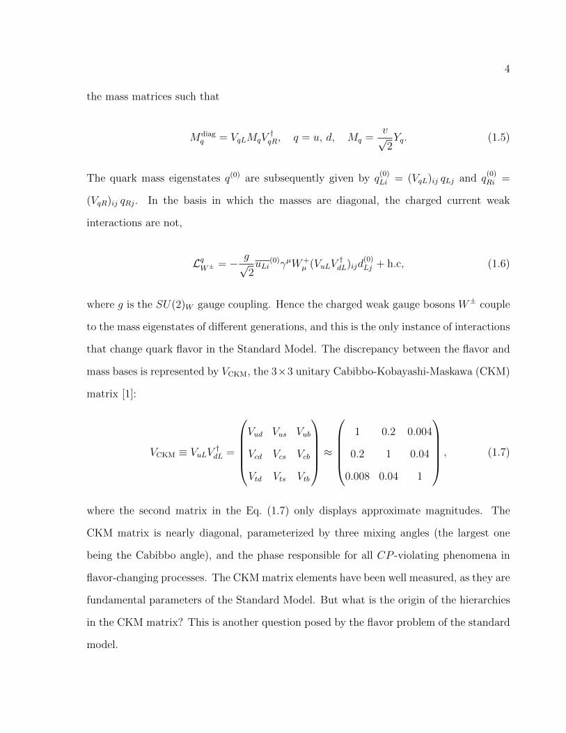
that change quark flavor in the Standard Model. The discrepancy between the flavor and
mass bases is represented by VCKM, the 3⇥3 unitary Cabibbo-Kobayashi-Maskawa (CKM)
matrix [1]:
VCKM ⌘ VuLV†dL
=
0
BBBB@
Vud Vus Vub
Vcd Vcs Vcb
Vtd Vts Vtb
1
CCCCA⇡
0
BBBB@
1 0.2 0.004
0.2 1 0.04
0.008 0.04 1
1
CCCCA, (1.7)
where the second matrix in the Eq. (1.7) only displays approximate magnitudes. The
CKM matrix is nearly diagonal, parameterized by three mixing angles (the largest one
being the Cabibbo angle), and the phase responsible for all CP -violating phenomena in
flavor-changing processes. The CKMmatrix elements have been well measured, as they are
fundamental parameters of the Standard Model. But what is the origin of the hierarchies
in the CKM matrix? This is another question posed by the flavor problem of the standard
model.
5
It is a possibility that the observed hierarchy of fermion masses and mixing angles
originates from the spontaneous breaking of a new horizontal flavor symmetry, GF . Ideally
only the Yukawa couplings for the third generation are allowed by the horizontal symmetry,
thereby accounting for the large, order-one top quark Yukawa coupling. The horizontal
symmetry is sequentially broken at energy scales µi through a series of nested subroups
Hi, such that
GF
µ1�! H1
µ2�! H2
µ3�! . . . for µ1 > µ2 > µ3. (1.8)
Here µi ⌘ h�ii /MF , where �i is the flavon field whose vev breaksHi�1 to Hi, andMF is the
ultraviolet cuto↵ of GF [3]. The hierarchical structure of the Yukawa couplings is achieved
on account of the di↵ering energy scales that are associated with the various stages of
symmetry breaking h�ii. Of course, a model with a horizontal symmetry is successful if it
yields Yukawa textures that are phenomenologically viable.
The literature contains many studies in which a horizontal symmetry is introduced to
obtain the hierarchical structure of the fermion masses. Models have been proposed with
Abelian [5, 6] and non-Abelian [7, 8, 9, 10, 11] continuous and discrete symmetries. One
type of particularly successful model considered in the literature assumes the continuous,
global symmetry GF = U(2) [12, 13, 14].These models involve fields in 1, 2 and 3 dimen-
sional representations (reps), with quarks and leptons embedded into 2 � 1 dimensional
reps. This allows for an order-one top quark Yukawa coupling, as the third generation fields
are treated di↵erently. A set of flavons (the symmetry-breaking fields) appears in all three
of these representations. The U(2) group contains the multiplication rule 2 ⌦ 2 = 3 � 1,
which results in a symmetric and antisymmetric decomposition of the Yukawa matrices
6
for first and second generation fields so that the Yukawa sector takes the form:
YU,D,E ⇠
0
B@Sab + Aab �a
�a 1
1
CA . (1.9)
Here �a, Sab and Aab are a set of flavon fields, where � is a U(2) doublet, S is a symmetric
U(2) triplet and A is an antisymmetric U(2) singlet. The U(2) symmetry is broken to
a U(1) subgroup that rotates all first generation fields by a phase. This forbids Yukawa
couplings involving first generation fields. The residual U(1) symmetry is broken at a lower
scale to nothing; this sequential symmetry breaking produces a hierarchy in the Yukawa
couplings.
Although a horizontal U(2) symmetry explains the observed hierarchy of fermion
masses, it is not the most minimal symmetry. In Refs. [3, 4], Aranda, Carone and Lebed
consider the smallest discrete flavor group that predicts the same form of the Yukawa
textures. This is accomplished by assuming the symmetry GF = T0⇥Z3 and the breaking
pattern
T0⇥ Z3
✏�! Z
D
3✏0
�! nothing. (1.10)
Here Z3 is a discrete Abelian subgroup of U(1) and T0 is the double tetrahedral group,
the smallest discrete subgroup of SU(2) with 1, 2 and 3 dimensional reps and the multi-
plication rule 2⌦ 2 = 3� 1. T 0 contains 24 elements: 12 elements that correspond to the
12 proper rotations that take a regular tetrahedron into coincidence with itself, while the
remaining 12 elements result from a rotation by 2⇡ of the first set, which produces a factor
of �1 in the even-dimensional reps. The T0⇥ Z3 flavor group contains the diagonal ZD
3
subgroup, which is responsible for rotating all first-generation matter fields by a phase.
When the T0⇥ Z3 symmetry is broken to Z
D
3 , it is assumed that the doublet and triplet
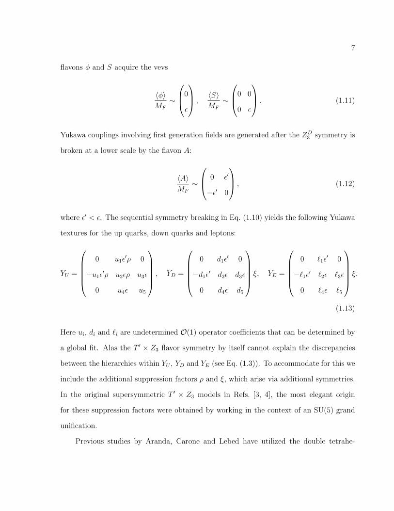
7
flavons � and S acquire the vevs
h�i
MF
⇠
0
B@0
✏
1
CA ,hSi
MF
⇠
0
B@0 0
0 ✏
1
CA . (1.11)
Yukawa couplings involving first generation fields are generated after the ZD
3 symmetry is
broken at a lower scale by the flavon A:
hAi
MF
⇠
0
B@0 ✏
0
�✏0 0
1
CA , (1.12)
where ✏0 < ✏. The sequential symmetry breaking in Eq. (1.10) yields the following Yukawa
textures for the up quarks, down quarks and leptons:
YU =
0
BBBB@
0 u1✏0⇢ 0
�u1✏0⇢ u2✏⇢ u3✏
0 u4✏ u5
1
CCCCA, YD =
0
BBBB@
0 d1✏0 0
�d1✏0
d2✏ d3✏
0 d4✏ d5
1
CCCCA⇠, YE =
0
BBBB@
0 `1✏0 0
�`1✏0`2✏ `3✏
0 `4✏ `5
1
CCCCA⇠.
(1.13)
Here ui, di and `i are undetermined O(1) operator coe�cients that can be determined by
a global fit. Alas the T0⇥ Z3 flavor symmetry by itself cannot explain the discrepancies
between the hierarchies within YU , YD and YE (see Eq. (1.3)). To accommodate for this we
include the additional suppression factors ⇢ and ⇠, which arise via additional symmetries.
In the original supersymmetric T0⇥ Z3 models in Refs. [3, 4], the most elegant origin
for these suppression factors were obtained by working in the context of an SU(5) grand
unification.
Previous studies by Aranda, Carone and Lebed have utilized the double tetrahe-
8
dral group to build flavor models that provide a successful description of charged fermion
masses and the CKM mixing elements. However these theories were constructed nearly
two decades ago, back when it was assumed that weak-scale supersymmetry was the likely
solution to the hierarchy problem. However the LHC has yet to produce any results that
would confirm the existence of supersymmetry, thereby reducing confidence in supersym-
metry as a key ingredient in tackling issues raised by the standard model. Instead we
ask the question, how well do the T0 flavor models in Refs. [3, 4] work if there is no
supersymmetry below the Planck scale?
In our study discussed in Chapter 2, we numerically evolve the Yukawa matrices
in Eq. (2.13) using the one-loop, nonsupersymmetric renormalization groups equations
(RGEs). The RGEs are run down from the from the flavor scale, MF , to the weak scale,
mZ (the mass of the Z boson). The flavor scale is varied from the TeV scale to the Planck
scale, MP l, and the Yukawa matrices are diagonalized at the weak scale. We perform
global fits to the charged fermion masses and the CKM angles. Our results indicate that
T0 models without supersymmetry provide viable phenomenological results for a wide range
of MF , with a preference for values closer to the TeV scale than the Planck scale. However
the feasibility of MF ⇠ MP l is consistent with the possibility that there is no new physics
between the weak and gravitational scales. The lowest MF are further constrained by
flavor-changing-neutral-current (FCNC) processes that receive contributions from physical
components of the flavon fields, thus providing indirect probes of the model.
In building flavor models, we aim to explain the origin of the Yukawa couplings. Sim-
ilarly we may also attempt to explain the origins of the Standard Model’s gauge couplings,
↵1, ↵2 and ↵3, which characterize the strength of the electromagnetic, weak and strong
forces. The coupling constants are dependent on the energy scale, µ, at which one observes
9
them, and the running of the couplings is encoded in the renormalization group equations:
dgi
dt=
gi
16⇡2
"big
2i+
1
16⇡2
X
j=1
bijg2ig2j�
X
j=U,D,E
aijg2itr[YjY
†j]
!#, (1.14)
where t = lnµ is the log of the renormalization scale, ↵i = g2i/4⇡, bi and bij are the
beta function coe�cients and aij are the coe�cients for the Yukawa matrices Yi (though
in practice only the top quark Yukawa coupling needs to be taken into account since it
is significantly larger than the other Yukawa couplings). The evolution of the Standard
Model RGE’s from the weak scale to the Planck scale is given in Fig. 1.1.
α1-1
α2-1
α3-1
1 104 108 1012 1016
0
10
20
30
40
50
60
μ (GeV)
α-1
FIG. 1.1: Running of the Standard Model gauge couplings from the weak scale to the Planckscale.
Fig. 1.1 is suggestive of unification, and with additional physics beyond the Standard
Model it is possible that the gauge couplings meet at a high scale. In this case hypercharge
would be unified with the strong and weak forces, which would explain why fundamental
particles carry electric charges that appear to be exact multiples of 1/3 of the elementary
charge, as opposed to other arbitrary numbers. Charge quantization can be addressed
through the introduction of a grand unified theory (GUT) in which the SM gauge group is
embedded in a larger underlying gauge group (such as SU(5)) with a single gauge coupling
constant [15]. Quarks and leptons are placed together in irreducible representations of the
10
underlying group and are related by its symmetries. For instance if we embed the SM
in SU(5), the fermions fit neatly into its anomaly-free chiral 5 � 10 representation. The
underlying group is then broken to SU(3)⇥SU(2)⇥U(1) at some high scale, typically in
the 1014 � 1016 GeV range [16]. Above this scale all fermions and their interactions would
appear very much alike, and thus the electromagnetic, weak and strong forces would all
come together (up to normalization factors) at the GUT scale.
Although a tantalizing idea, grand unified theories have their shortcomings as well.
Many GUT models explicitly break the baryon number symmetry, allowing protons to
decay, in contradiction with current experimental evidence [17]. In supersymmetric GUT
models, an extreme fine-tuning of parameters is required to produce a large mass splitting
in Higgs multiplets, called the “doublet-triplet splitting problem” [18], to keep the SM
Higgs doublet much lighter than the GUT scale. However, there is an alternative frame-
work in which the gauge couplings assume a common value at a high energy scale without
calling for conventional grand unification. Instead we assume the existence of a universal
Landau pole in which the gauge couplings blow up at a common scale ⇤ in the ultraviolet:
↵�11 (⇤) = ↵
�12 (⇤) = ↵
�13 (⇤) = 0. (1.15)
A universal Landau pole may arise in models with composite gauge bosons. For instance,
the QED Lagrangian with radiative corrections contains the terms
L � �1
4Z(µ)F µ⌫
Fµ⌫ + g0Aµ �µ . (1.16)
If the photon were composite, we would expect the photon’s wave-function renormalization
factor to vanish at the compositeness scale, i.e., Z(⇤comp) = 0, indicating that the photon
has become nondynamical. Redefining the fields and couplings so that the gauge field’s
11
kinetic term retains its canonical form,
L � �1
4F
µ⌫Fµ⌫ +
g0pZ(µ)
Aµ �µ , (1.17)
the gauge coupling is given by g(µ) = g0/
pZ(µ), which blows up as the wave-function
renormalization factor goes to zero at the compositeness scale. This gives plausibility to
the boundary condition in Eq. (1.15).
For a universal Landau pole to be achieved all the gauge couplings must be asymp-
totically non-free, but since this is not the case for the SU(3) coupling in the minimal
supersymmetric standard model (MSSM), additional matter is necessary. The simplest
implementation of this idea is presented in Ref. [18], in which the MSSM is augmented
by an additional vector-like generation of matter fields at the TeV scale. In Chapter 3 of
this thesis we revisit this minimal scenario and find extensions that produce more viable
phenomenological results.
There are two scales to consider: the scale of the new vector-like matter, mV , and
the susy-breaking scale, msusy. In the previous literature the two scales were set equal to
one another [18], although we allow them to vary independently in our study. For a given
choice of mV and msusy, we fix the blow-up scale ⇤ by the requirement that the correct
value of the fine structure constant at the weak scale is reproduced. We then compute the
weak scale values of ↵�13 and the Weinberg angle sin2
✓W up to theoretical uncertainties.
A viable solution is obtained if a value of mV and msusy can be found in which both
sin2✓W (mZ) and ↵
�13 (mZ) are consistent with the data.
At the Landau pole in Eq. (1.15) the gauge couplings are in the non-perturbative
regime, where the RGEs cannot be trusted. Instead we impose the boundary condition
↵1(⇤) = ↵2(⇤) = ↵3(⇤) = 10, values that are barely perturbative. This still e↵ectively
results in a Landau pole since for ↵(⇤) = 10 and ↵(⇤actual) = 1, there is negligible
12
di↵erence between ⇤ and ⇤actual, as the couplings rapidly increase as the renormalization
scale is increased. To determine the theoretical uncertainty we vary ↵i independently
between 1 and 100 at the blow-up scale and find that the low-energy coupling constants
are nearly independent of the precise choice of boundary conditions, as long as the couplings
are large at ⇤. This insensitivity is due to the existence of an infrared fixed point in the
RGE for the ratios of the gauge couplings [19].
As the minimal scenario described above was studied more than two decades ago,
we reproduce it with up-to-date experimental data, but find that it requires values of
either mV or msusy that are in some tension with current LHC bounds. Thus we consider
extensions of the minimal scenario, particularly by including a small number of additional
complete SU(5) multiplets of vector-like matter, as this is known to preserve successful
unification. This leads to solutions for mV that are beyond the reach of the LHC, but
potentially within reach of a 100 TeV future hadron collider for some choices of msusy. We
consider the possibility that the new matter fields transform under an additional gauge
group that is constrained by the same ultraviolet boundary condition. In that case the
heavy fields could fall in irreducible representations of the new gauge group, explaining
the multiplicity of new particles required to achieve the Landau pole. We explore the
consequences of the heavy matter sector being vector-like or chiral under the new gauge
group.
We have discussed scenarios in which the three gauge couplings unify, but there is
a fourth fundamental force to consider: gravity. The electromagnetic, weak and strong
forces are successfully described in a quantum mechanical framework, while our current
understanding of gravity is based on Einstein’s general theory of relativity, which is derived
within the framework of classical physics. To unify gravity with the other forces we would
first need to find a consistent quantum mechanical description.
Quantizing gravity necessitates the existence of a force-carrying particle akin to the
13
photon of the electromagnetic interaction; this can be accomplished with the introduction
of the spin-two massless graviton. But when applying standard protocols of quantum field
theory to the graviton, the resulting theory is not renormalizable and consequently the
predictivity of the theory is lost. In a renormalizeable theory there exists a finite number
of relevant parameters, capable of being measured via experiment, which encodes all the
physics of the theory at a particular energy scale. For instance in quantum electrodynamics
these parameters are the mass and charge of the electron. Then the number of divergences
are finite and may be absorbed into the renormalization of these parameters. In the case
of gravity the number of divergences is not finite [20]. The Einstein-Hilbert term is given
by
SEH =1
16⇡GN
ZdDxR
p�g =
1
22
ZdDxR
p�g (1.18)
where GN is Newton’s gravitational constant, is related to the d-dimensional Planck
length, g = det(|gµ⌫ |) is the determinant of the metric tensor andR is the Ricci (curvature)
scalar of general relativity. To expand the gravitational action around flat space we write
gµ⌫ = ⌘µ⌫ + hµ⌫ , where ⌘µ⌫ is the flat-space metric and hµ⌫ is a perturbation about it.
Then an expansion in the action results in an infinite series of the form
SEH ⇠1
2
1X
n=0
ZdDx(@h)2(h)n, (1.19)
where 2 has units of [L]D�2 and so is not dimensionless for D > 2 [20]. Each term in the
expansion receives divergent loop contributions involving lower order terms, requiring an
ever-increasing number of counterterms to cancel the divergences. Accordingly we would
need to specify an infinite set of parameters before the theory is fixed, wherein the process
of renormalization fails.
Besides nonrenormalizeability, quantum gravity also faces the problem of time. Quan-
14
tum mechanics takes the flow of time to be universal and absolute, as it acts as an inde-
pendent background through which states evolve. The Hamiltonian operator is responsible
for generating infinitesimal translations of quantum states through time. In contrast gen-
eral relativity assumes that time is a dynamical variable. But this would require the
Hamiltonian to vanish, producing an absence of dynamics of quantum states.
String theory has commonly been called upon to resolve some of these issues. It
introduces a new length scale, related to the string tension, at which particles are no longer
pointlike. Oscillations of the string manifest themselves as new symmetries (particularly
supersymmetry) that reduce the infinite parameters to a finite set. However as it was
pointed out above there is an increasing loss of confidence in supersymmetry, as the LHC
has yet to produce any results that confirm its existence. Furthermore, string theory
introduces a huge number of ground state vacua, perhaps ⇠ 10500 [21], so there is a
price to pay in making quantum gravity finite. Thus we focus on another possibility: the
emergence of gravity as the e↵ective description of a massless composite spin-two state.
The possibility of emergent long-range interactions in quantum field theory is not
limited to gravity. In Ref. [22], Bjorken argued that a four-fermion interaction of the form
Lint = GF ( �µ )( �µ ) gives rise to a massless spin-one composite state with interactions
akin to the photon in electrodynamics. During the development of the theory of the strong
sector, it was briefly considered that quantum chromodynamics emerged as consequence
of color confinement imposed via a constraint of vanishing color current, rather than the
other way around [24, 25]. Since the Standard Model provided a successful description
of the electroweak and strong interactions, the existence of emergent gauge interactions
was no longer necessary to explain existing phenomena. However the Standard Model has
yet to successfully incorporate general relativity, and so the paradigm of emergent gravity
remains compelling. Much of the activity in this area has been inspired by Ref. [26],
in which Sakharov pointed out that the dynamics of spacetime emerge in a generally
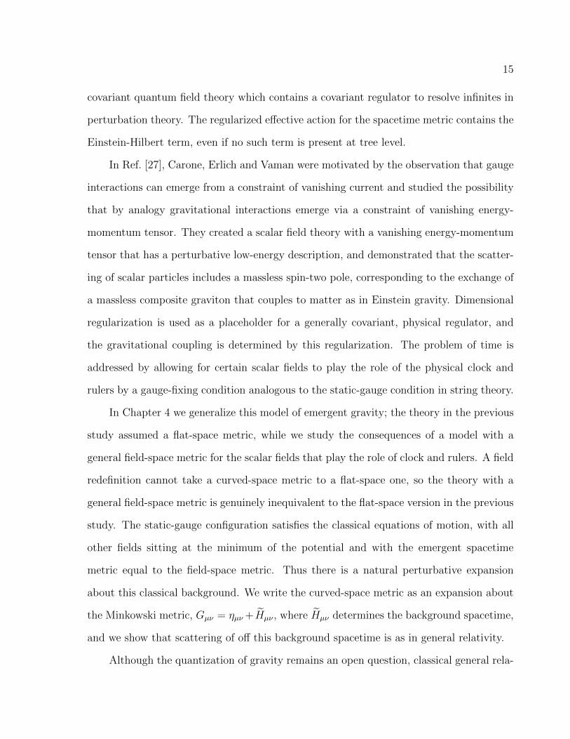
15
covariant quantum field theory which contains a covariant regulator to resolve infinites in
perturbation theory. The regularized e↵ective action for the spacetime metric contains the
Einstein-Hilbert term, even if no such term is present at tree level.
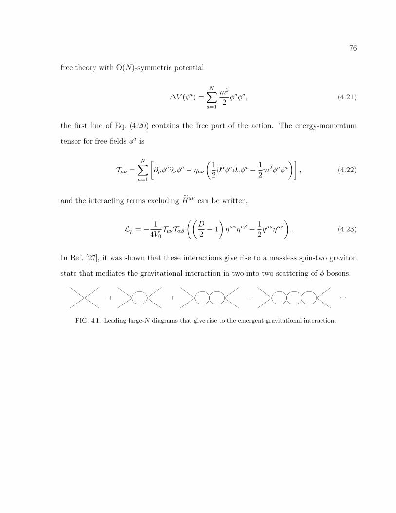
In Ref. [27], Carone, Erlich and Vaman were motivated by the observation that gauge
interactions can emerge from a constraint of vanishing current and studied the possibility
that by analogy gravitational interactions emerge via a constraint of vanishing energy-
momentum tensor. They created a scalar field theory with a vanishing energy-momentum
tensor that has a perturbative low-energy description, and demonstrated that the scatter-
ing of scalar particles includes a massless spin-two pole, corresponding to the exchange of
a massless composite graviton that couples to matter as in Einstein gravity. Dimensional
regularization is used as a placeholder for a generally covariant, physical regulator, and
the gravitational coupling is determined by this regularization. The problem of time is
addressed by allowing for certain scalar fields to play the role of the physical clock and
rulers by a gauge-fixing condition analogous to the static-gauge condition in string theory.
In Chapter 4 we generalize this model of emergent gravity; the theory in the previous
study assumed a flat-space metric, while we study the consequences of a model with a
general field-space metric for the scalar fields that play the role of clock and rulers. A field
redefinition cannot take a curved-space metric to a flat-space one, so the theory with a
general field-space metric is genuinely inequivalent to the flat-space version in the previous
study. The static-gauge configuration satisfies the classical equations of motion, with all
other fields sitting at the minimum of the potential and with the emergent spacetime
metric equal to the field-space metric. Thus there is a natural perturbative expansion
about this classical background. We write the curved-space metric as an expansion about
the Minkowski metric, Gµ⌫ = ⌘µ⌫+ eHµ⌫ , where eHµ⌫ determines the background spacetime,
and we show that scattering of o↵ this background spacetime is as in general relativity.
Although the quantization of gravity remains an open question, classical general rela-
16
tivity continues to be an excellent description of the universe at macroscopic scales provided
that one additional ingredient is assumed: dark matter, a hypothetical form of matter that
does not directly interact with observable electromagnetic radiation but believed to ac-
count for approximately 85% of the total matter in the universe [28]. Yet this mystery
has no place in the Standard Model, despite a variety of astrophysical phenomena im-
plying its existence. The primary evidence for dark matter arises from galactic rotation
curves, which illustrate how the orbital velocity of visible stars and gas in a galaxy varies
with their distance from the galaxy’s center. From Kepler’s Second Law, it is expected
that the rotational velocities of stars in spiral galaxies would decrease with distance from
the galactic center; however the rotational velocities have been observed to remain flat
with increasing distance. This inconsistency suggests that each galaxy is surrounded by
significant amounts of non-luminous matter (dark matter).
The primary candidate for dark matter is some new sort of elementary particle that has
yet to be discovered; candidates include weakly-interacting massive particles (WIMPs), ax-
ions (hypothetical particles postulated to resolve the strong charge-parity problem in quan-
tum chromodynamics), sterile neutrinos (heavy neutrinos without electroweak quantum
numbers that are motivated to explain the observed neutrino masses), and in supersym-
metric models, the LSP (lightest supersymmetric partner). There are many experiments
aimed at detecting dark matter, divided into two classes: direct detection experiments
(including LUX [29], XENON [30], CDMS [31]), which observe the e↵ects of dark matter
collisions with atomic nuclei within a detector, and indirect detection experiments (includ-
ing PAMELA [32] and IceCube [33]), which search for the products from the annihilation
or decay of dark matter particles in the galaxy, including excessive bursts of gamma rays,
positrons or antiprotons.
All dark matter models have to annihilate a su�cient amount of dark matter so that
the correct relic density is obtained. Dark matter “freezes out” when its interactions prob-
17
ability per unit time falls below the expansion rate of the universe [34]. The literature
contains many diverse dark matter models which reproduce the desired relic density, al-
though they all usually contain three components: the visible sector that at a minimum
includes all the standard model fields, the dark sector which consists of a collection of
fields that communicate very weakly with the visible sector, and the messenger or portal
sector which enables a coupling between the previous two sectors. Dark matter models
have been proposed with Abelian and non-Abelian symmetries; see Refs. [35, 36, 37, 38, 39]
for examples of the former and Refs. [40, 41, 42, 43, 44, 45, 46] for the latter. There are
a wide variety of proposed portals between the dark and visible sectors, including kinetic
mixing portals, Higgs portals, and vector-like fermion portals.
In Chapter 5 we consider fermionic dark matter that is charged under the simplest
non-Abelian dark gauge group, and focus on the case where the vector-like fermion portal
is dominant. Such a portal consists of vector-like fermions that are charged under the dark
gauge group but contain the quantum numbers of some standard model particle (in our
case, the right-handed electron), so that communication between the dark and visible sec-
tors can occur via mass mixing. In our model, the dark gauge boson couples to a vector-like
state that mixes with standard model leptons after the dark and visible gauge symmetries
of the theory are spontaneously broken. However, lepton-flavor-violating processes emerge
when the vector-like lepton mixes with all three standard model flavors. Consequently,
there are bounds on vector-like heavy leptons that exceed 100 TeV [47]. But to obtain a
su�cient dark matter annihilation cross section to a standard model lepton, the mixing
angle cannot be too small, which implies that the vector-like leptons cannot be arbitrar-
ily heavy. To work around the stringent lower bounds on heavy vector-like leptons that
arise from lepton-flavor-violating processes, we identify a mechanism, based on discrete
symmetries, that we call “flavor sequestering.” This allows for mixing between the vector-
like leptons and a single standard model lepton flavor exclusively (the remaining standard
18
model lepton flavors may only mix with each other). Thus lepton flavor violation is sup-
pressed, providing for vector-like fermion portal sectors that are lighter. Then the mixing
angle between the vector-like lepton and the chosen lepton flavor can be large enough so
that an adequate scattering cross section is obtained from dark matter annihilation to a
lepton-anti-lepton pair. The vector-like fermion portal we present is renormalizeable and
completely specified; we explicitly investigate the flavor structure dictating the mixing be-
tween the exotic and standard model fields and the resulting phenomenology. Specifically,
we look for regions of parameter space that successfully reproduce the dark matter relic
density and satisfy current direct detection bounds.
To recap: this thesis addresses a variety of issues that are not resolved by the Stan-
dard Model. In Chapter 2, we explain the observed hierarchies in the elementary fermion
mass spectrum via a model based on the double tetrahedral group, a subgroup of SU(2),
without relying on supersymmetry. In Chapter 3, we consider an alternative to conven-
tional unification in which the electromagnetic, weak and strong couplings blow up at a
common Landau pole and consider extensions of the minimal scenario, to see if there are
cases that might be probed at a future 100 TeV collider. In Chapter 4, we turn to the
issue of quantum gravity, generalizing a composite graviton model to the case of curved
spacetime backgrounds. In Chapter 5, we consider a model with fermionic dark matter
that communicates with the Standard Model via a vector-like fermion portal. We present
a framework based on symmetries that allows the mixing between the dark and visible
sectors to be non-negligible, while simultaneously suppressing unwanted flavor-changing
processes. Lastly we summarize our conclusions in Chapter 6.
CHAPTER 2
Flavor from the double tetrahedral
group without supersymmetry 1
In this chapter we consider a class of previous flavor models, relaxing the assumption
of supersymmetry and allowing the flavor scale to float anywhere between the weak and
Planck scales. We perform global fits to the charged fermion masses and CKM angles,
and consider the dependence of the results on the unknown mass scale of the flavor sector.
We find that the typical Yukawa textures in these models provide a good description of
the data over a wide range of flavor scales, with a preference for those that approach
the lower bounds allowed by flavor-changing-neutral-current constraints. Nevertheless,
the possibility that the flavor scale and Planck scale are identified remains viable. We
present models that demonstrate how the assumed textures can arise most simply in a
non-supersymmetric framework.
1Work previously published in C. D. Carone, S. Chaurasia and S. Vasquez, “Flavor from the doubletetrahedral group without supersymmetry,” Phys. Rev. D 95, no. 1, 015025 (2017) [arXiv:1611.00784[hep-ph]].
19
20
2.1 Introduction
There is a vast literature on models that attempt to explain the observed hierarchy
of fermion masses by means of horizontal symmetries. In this chapter, we revisit one such
model, proposed by Aranda, Carone and Lebed, based on the double tetrahedral group
T0 [3, 4]. Prior to this work, it had been shown that supersymmetric grand unified theories
with U(2) flavor symmetry predict simple forms for the Yukawa matrices, ones that provide
a successful description of charged fermion masses and the Cabibbo-Kobayashi-Maskawa
(CKM) mixing matrix [12, 14]. The authors of Ref. [3, 4] posed a simple question: What
is the smallest discrete flavor group that predicts the same form for the Yukawa textures?
The answer to this question was determined by the specific group theoretic properties of
U(2) that were utilized in the most successful U(2) models [14]:
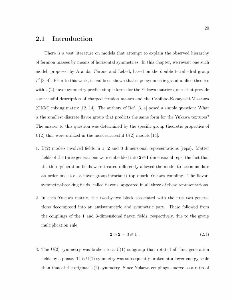
1. U(2) models involved fields in 1, 2 and 3 dimensional representations (reps). Matter
fields of the three generations were embedded into 2�1 dimensional reps; the fact that
the third generation fields were treated di↵erently allowed the model to accommodate
an order one (i.e., a flavor-group-invariant) top quark Yukawa coupling. The flavor-
symmetry-breaking fields, called flavons, appeared in all three of these representations.
2. In each Yukawa matrix, the two-by-two block associated with the first two genera-
tions decomposed into an antisymmetric and symmetric part. These followed from
the couplings of the 1 and 3-dimensional flavon fields, respectively, due to the group
multiplication rule
2⌦ 2 = 3� 1 . (2.1)
3. The U(2) symmetry was broken to a U(1) subgroup that rotated all first generation
fields by a phase. This U(1) symmetry was subsequently broken at a lower energy scale
than that of the original U(2) symmetry. Since Yukawa couplings emerge as a ratio of
21
a symmetry-breaking scale to a cut o↵, the sequential breaking of the flavor symmetry
explains why the Yukawa couplings associated with first generation were smaller than
those of the heavier generations.
The group T0 is special in that it is the smallest discrete group that has 1, 2 and 3-
dimensional representations, as well as the multiplication rule 2 ⌦ 2 = 3 � 1. We will
briefly review the representations and multiplication rules for T0 symmetry in Sec. 2.2.
Following Ref [3, 4], the appropriate symmetry breaking sequence is achieved if the flavor
group includes an Abelian factor, so that GF = T0⇥Z3. Then the breaking pattern of the
U(2) model
U(2)✏
�! U(1)✏0
�! nothing, (2.2)
is mimicked by
T0⇥ Z3
✏�! Z
D
3✏0
�! nothing. (2.3)
Here we have indicated the scale of each symmetry breaking via the dimensionless pa-
rameters ✏ and ✏0, which represent the ratio of a symmetry-breaking vacuum expectation
value (vev) to the cut o↵ of the e↵ective theory. We refer to the cut o↵ as the flavor scale,
MF , henceforth. A useful way to understand the connection between Eq. (2.2) and (2.3)
is to consider the SU(2)⇥U(1) subgroup of U(2); The T 0 factor is a subgroup of the SU(2)
factor while Z3 is a subgroup of the U(1). The Z3 factor remaining after the first step in
the symmetry-breaking chain in Eq. (2.3) also transforms all first generation fields by a
phase and will be specified later. The T0⇥ Z3 model defined in this way reproduces the
successful Yukawa textures of the U(2) models, but with a much smaller symmetry group.
For other productive applications of T 0 symmetry in flavor model building, we refer the
reader to Ref. [48].
The T0 models of Refs. [3, 4] were constructed more than 16 years ago, when it was
22
widely assumed that weak-scale supersymmetry was the likely solution to the gauge hier-
archy problem. The numerical study of the Yukawa textures in these references assumed
supersymmetric renormalization group equations to relate the predictions of the theory
at the flavor scale MF to those at observable energies. Superpartners were taken to have
masses just above the electroweak scale, while MF was identified with the scale of super-
symmetric grand unification, ⇠ 2 ⇥ 1016 GeV. The latter choice was motivated by the
most elegant T 0 models, which were formulated in the context of an SU(5) grand unified
theory. Some of the essential features of the Yukawa textures followed from the combined
restrictions of the flavor and grand unified symmetries.
At the present moment, however, the status of weak-scale supersymmetry as a nec-
essary ingredient in model building is far less certain. The latest data from the LHC has
found no evidence for supersymmetry. Of course, this may simply mean that the scale of
the superpartner masses is slightly higher than what one might prefer from the perspective
of naturalness; this interpretation would have little e↵ect on the results of Refs. [3, 4]. On
the other hand, the LHC may be hinting that there is no necessary connection between the
weak scale and the scale of supersymmetry breaking. In this case, one might entertain the
possibility that the supersymmetry breaking scale is associated with the only higher phys-
ical mass scale whose existence is well established: the Planck scale. For example, it has
been suggested in Ref. [49] that the shallowness of the Higgs potential may be explained
by Planck-scale supersymmetry breaking, assuming that supersymmetry is still relevant
for a quantum gravitational completion. This latter assumption itself has been challenged
in Ref. [50], where it has been noted that there are consistent string theories that are fun-
damentally non-supersymmetric and whose low-energy limit could include the standard
model. Whether supersymmetry is broken at the Planck scale, or not present at any scale,
one might attempt to address the hierarchy between the weak scale and Planck scale, for
example, by anthropic selection, or by Higgs field relaxation [51], or by mechanisms not yet
23
known. Alternatively, one might pursue the idea that quantum gravitational physics does
not contribute to scalar field quadratic divergences in the way that one expects naively
from e↵ective field theory arguments [52]. In this chapter, we remain completely agnostic
on the issue of naturalness. We instead investigate a question that can be addressed in a
more definitive and quantitative way: how well do the T 0 flavor models in Refs. [3, 4] work
if there is no supersymmetry below the Planck scale?
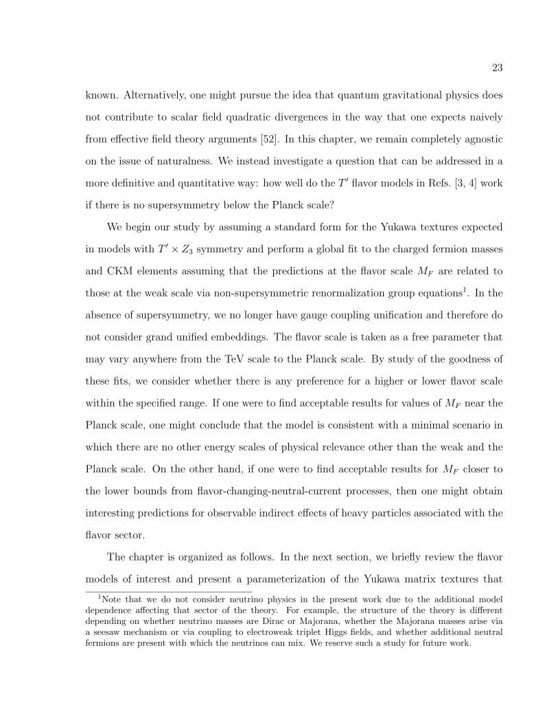
We begin our study by assuming a standard form for the Yukawa textures expected
in models with T0⇥ Z3 symmetry and perform a global fit to the charged fermion masses
and CKM elements assuming that the predictions at the flavor scale MF are related to
those at the weak scale via non-supersymmetric renormalization group equations1. In the
absence of supersymmetry, we no longer have gauge coupling unification and therefore do
not consider grand unified embeddings. The flavor scale is taken as a free parameter that
may vary anywhere from the TeV scale to the Planck scale. By study of the goodness of
these fits, we consider whether there is any preference for a higher or lower flavor scale
within the specified range. If one were to find acceptable results for values of MF near the
Planck scale, one might conclude that the model is consistent with a minimal scenario in
which there are no other energy scales of physical relevance other than the weak and the
Planck scale. On the other hand, if one were to find acceptable results for MF closer to
the lower bounds from flavor-changing-neutral-current processes, then one might obtain
interesting predictions for observable indirect e↵ects of heavy particles associated with the
flavor sector.
The chapter is organized as follows. In the next section, we briefly review the flavor
models of interest and present a parameterization of the Yukawa matrix textures that
1Note that we do not consider neutrino physics in the present work due to the additional modeldependence a↵ecting that sector of the theory. For example, the structure of the theory is di↵erentdepending on whether neutrino masses are Dirac or Majorana, whether the Majorana masses arise viaa seesaw mechanism or via coupling to electroweak triplet Higgs fields, and whether additional neutralfermions are present with which the neutrinos can mix. We reserve such a study for future work.
24
typically arise in these models at the flavor scale MF . In Sec. 2.3, we study the predictions
that follow from these textures by a non-supersymmetric renormalization group analysis,
including global fits to the current data on charged fermion masses and CKM elements.
In Sec. 2.4, we point out the largest indirect e↵ects of heavy flavor-sector particles on
flavor-changing-neutral current processes in the case where MF is low. In Sec. 3.4, we
address model building issues: supersymmetric models have two Higgs doublets (in order
to cancel anomalies) and have a superpotential that is constrained by holomorphicity;
these requirements are absent in the non-supersymmetric case. Hence, in this section we
show how the textures assumed in Sec. 2.3 may arise in non-supersymmetric T0 models.
In the final section, we summarize our conclusions.
2.2 Typical Yukawa textures from T-prime symmetry
The group T0 is discussed at length in Ref. [4]. Here we summarize only the most basic
properties relevant to the present discussion: The group has 24 elements. This includes 12
elements that correspond to the 12 proper rotations that take a regular tetrahedron into
coincidence with itself, with choices of Euler angles that are less than 2⇡. The remaining
12 elements are the first set times an element called R that corresponds to a 2⇡ rotation.
As we indicated earlier, T 0 has 1, 2 and 3-dimensional representations, that we specify
more precisely below. For odd-dimensional representations, R acts trivially and the action
of the group T0 is not distinguishable from that of the tetrahedral group T . For the even-
dimensional representations, however, R acts non-trivially; this reflects the fact that T 0 is
a subgroup of SU(2) and that spinors flip sign under a rotation by 2⇡.
The complete list of T 0 representations is as follows: there is a trivial singlet, 10, two
non-trivial singlets, 1±, three doublets, 20 and 2±, and one one triplet, 3. The di↵erent
singlet and doublet representations are distinguished by how they transform under a Z3
25
subgroup, generated by the group element called g9 in Ref. [4]. This is indicated by the
triality superscript; when we multiply representations, trialities add under addition modulo
three. Keeping this in mind, the rules for multiplying representations are then specified
by
1⌦R = R⌦ 1 for any rep R,
2⌦ 2 = 3� 1,
2⌦ 3 = 3⌦ 2 = 20� 2+
� 2�,
3⌦ 3 = 3� 3� 10� 1+
� 1�.
(2.4)
As we indicated in the Introduction, the models of interest are based on the flavor
group GF = T0⇥Z3, which includes a Z3 subgroup that rotates all first-generation matter
fields by a phase. We now identify that subgroup. In the models of Ref. [4], the first two
generations are assigned to the 20 representation2, in which the element g9 is given by
g9(20) =
0
B@⌘2 0
0 ⌘
1
CA , (2.5)
where ⌘ ⌘ e2⇡i/3. However, the matter fields may also transform under the Z3 factor
that commutes with T0. We represent charge assignments under this Z3 by an additional
triality index 0, + and �, corresponding to the phase rotations 1, ⌘ and ⌘2. The diagonal
subgroup of the Z3 subgroup generated by g9 and the Z3 factor that commutes with T0 is
the intermediate symmetry that we desire; we call this subgroup ZD
3 . If we assign the first
2This choice is motivated by the cancelation of discrete gauge anomalies. See Ref. [4] for details.
26
two generations to the rep 20�, then the action of ZD
3 is through powers of the product
g9(20) · ⌘2 =
0
B@⌘ 0
0 1
1
CA , (2.6)
which provides the desired first generation phase rotation.
Assigning the three generations of matter fields to the T0⇥ Z3 reps 20�
� 100 yields
the following transformation properties of the Yukawa matrices:
YU,D,E ⇠
0
B@[3�
� 10�] [20+]
[20+] [100]
1
CA . (2.7)
The models of interest include a set of flavon fields, Aab, �ab and Sab, which transform as
10�, 20+ and 3�, respectively. When the T0⇥ Z3 symmetry is broken to Z
D
3 , the doublet
and triplet flavons acquire the VEVs
h�i
MF
⇠
0
B@0
✏
1
CA ,hSi
MF
⇠
0
B@0 0
0 ✏
1
CA , (2.8)
where we use ⇠ when we omit possible order one factors. This is the most general pattern
of non-vanishing entries that is consistent with the unbroken ZD
3 symmetry defined by
Eq. (2.6). Yukawa couplings involving first-generation fields are generated only after the
ZD
3 symmetry is broken at a lower scale; in analogy to the U(2) models of Ref. [12, 14], it
is assumed that this is accomplished solely through the vev of the flavon Aab,
hAi
MF
⇠
0
B@0 ✏
0
�✏0 0
1
CA , (2.9)
27
where ✏0 < ✏. This sequential breaking T0⇥Z3
✏�! Z
D
3✏0
�! nothing yields a Yukawa texture
for the up quarks, down quarks and leptons of the form
YU,D,E ⇠
0
BBBB@
0 ✏0 0
�✏0✏ ✏
0 ✏ 1
1
CCCCA, (2.10)
where we’ve suppressed O(1) operator coe�cients.
The forms of the Yukawa matrices obtained in Eq. (2.10) are inadequate, given the
known di↵erences between the up-, down- and charged-lepton masses. The top quark
Yukawa coupling is of order one, while the all others are substantially smaller, suggesting
an additional overall suppression factor is desirable in YD and YE. Moreover, the hierarchy
of quark masses is more extreme in the up-quark sector than in the down; for example,
the quark mass ratios renormalized at the supersymmetric grand unified scale are given
approximately by [2]
md :: ms :: mb = �4 :: �2 :: 1 while mu :: mc :: mt = �
8 :: �4 :: 1, (2.11)
where � ⇡ 0.22 is the Cabibbo angle. This suggest that an additional suppression in the
1-2 block of YU is also desirable. We call these suppression factors ⇢ and ⇠, which modify
the textures of Eq. (2.10) as follows:
YU ⇠
0
BBBB@
0 ✏0⇢ 0
�✏0⇢ ✏ ⇢ ✏
0 ✏ 1
1
CCCCA, YD ⇠
0
BBBB@
0 ✏0 0
�✏0✏ ✏
0 ✏ 1
1
CCCCA⇠, YE ⇠
0
BBBB@
0 ✏0 0
�✏0✏ ✏
0 ✏ 1
1
CCCCA⇠. (2.12)
Clearly, the smallness of ⇢ and ⇠ does not follow directly from the assumed flavor symmetry
28
breaking, but requires additional symmetries and/or dynamics. In the U(2) models of
Refs. [12, 14] and the T0 models of Refs. [3, 4], ⇠ is assumed to arise from mixing in
the Higgs sector of the theory, while the origin of ⇢ is understood in terms of a grand
unified embedding. Flavon charge assignments under the unified gauge group can cause
Yukawa entries to arise at higher order in 1/MF than they would otherwise. In the non-
supersymmetric T0 models that we discuss in Sec. 3.4, we will neither have an extended
Higgs sector nor a grand unified embedding; we will, however, show how ⇢ and ⇠ may arise
simply by a small extension of the flavor symmetry.
All other di↵erences between YU , YD and YE can now be accommodated by the choice
of the undetermined O(1) operator coe�cients, identified according to naive dimensional
analysis. We generally require these to be between 1/3 and 3 in magnitude; the precise
range is a matter of taste, but our choice is consistent with the assumptions of Refs. [3, 4].
Variations in the operator coe�cients are then su�cient, for example, to account for
di↵erences between YD and YE that are attributed to group theoretic factors of 3 in grand
unified theories [53]. We parameterize the Yukawa matrices in terms of coe�cients ui, di
and `i as follows:
YU =
0
BBBB@
0 u1✏0⇢ 0
�u1✏0⇢ u2✏⇢ u3✏
0 u4✏ u5
1
CCCCA, YD =
0
BBBB@
0 d1✏0 0
�d1✏0
d2✏ d3✏
0 d4✏ d5
1
CCCCA⇠, YE =
0
BBBB@
0 `1✏0 0
�`1✏0`2✏ `3✏
0 `4✏ `5
1
CCCCA⇠.
(2.13)
These forms will be used to define the Yukawa matrices at the flavor scale MF in the
numerical study presented in the following section.
29
2.3 Numerical analysis
We numerically evolve the Yukawa matrices in Eq. (2.13), using the one-loop, non-
supersymmetric renormalization group equations (RGEs). The flavor scale MF is taken to
be variable, while the scale of observable energies is chosen to be the mass of the Z boson,
mZ . We omit all weak-scale threshold corrections. The RGEs are given by [54]
dgi
dt=
bSMi
16⇡2g3i, (2.14)
dYU
dt=
1
16⇡2
�
X
i
cSMi
g2i+
3
2YUY
†U�
3
2YDY
†D+ Y2(S)
!YU , (2.15)
dYD
dt=
1
16⇡2
�
X
i
c0SMi
g2i+
3
2YDY
†D�
3
2YUY
†U+ Y2(S)
!YD , (2.16)
dYE
dt=
1
16⇡2
�
X
i
c00SMi
g2i+
3
2YEY
†E+ Y2(S)
!YE, (2.17)
where
Y2(S) = Tr[3YUY†U+ 3YDY
†D+ YEY
†E] . (2.18)
Here, the gi are the gauge couplings, YU , YD and YE are the Yukawa matrices, and t = lnµ
is the log of the renormalization scale. The SU(5) normalization of g1 is assumed. In the
absence of supersymmetry [54],
bSMi
=
✓41
10, �
19
6, �7
◆, (2.19)
and
cSMi
=
✓17
20,
9
4, 8
◆, c
0SMi
=
✓1
4,
9
4, 8
◆, c
00SMi
=
✓9
4,
9
4, 0
◆. (2.20)
30
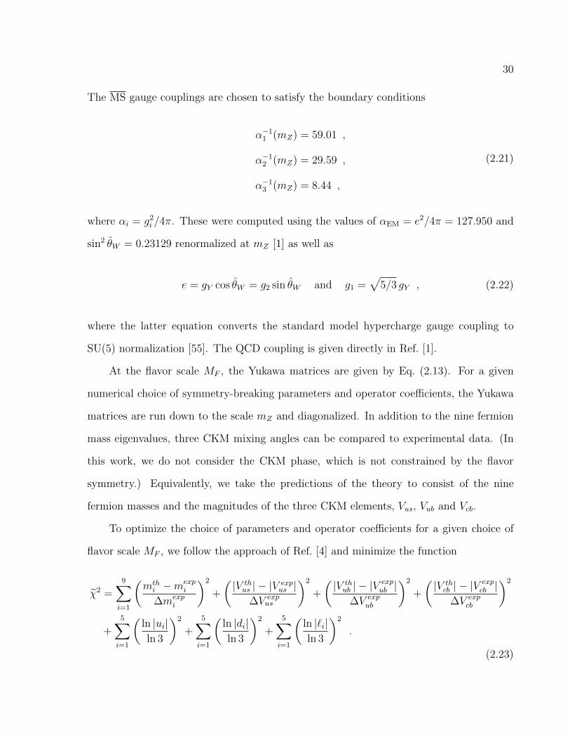
The MS gauge couplings are chosen to satisfy the boundary conditions
↵�11 (mZ) = 59.01 ,
↵�12 (mZ) = 29.59 ,
↵�13 (mZ) = 8.44 ,
(2.21)
where ↵i = g2i/4⇡. These were computed using the values of ↵EM = e
2/4⇡ = 127.950 and
sin2✓W = 0.23129 renormalized at mZ [1] as well as
e = gY cos ✓W = g2 sin ✓W and g1 =p
5/3 gY , (2.22)
where the latter equation converts the standard model hypercharge gauge coupling to
SU(5) normalization [55]. The QCD coupling is given directly in Ref. [1].
At the flavor scale MF , the Yukawa matrices are given by Eq. (2.13). For a given
numerical choice of symmetry-breaking parameters and operator coe�cients, the Yukawa
matrices are run down to the scale mZ and diagonalized. In addition to the nine fermion
mass eigenvalues, three CKM mixing angles can be compared to experimental data. (In
this work, we do not consider the CKM phase, which is not constrained by the flavor
symmetry.) Equivalently, we take the predictions of the theory to consist of the nine
fermion masses and the magnitudes of the three CKM elements, Vus, Vub and Vcb.
To optimize the choice of parameters and operator coe�cients for a given choice of
flavor scale MF , we follow the approach of Ref. [4] and minimize the function
e�2 =9X
i=1
✓m
th
i�m
exp
i
�mexp
i
◆2
+
✓|V
th
us|� |V
exp
us|
�Vexp
us
◆2
+
✓|V
th
ub|� |V
exp
ub|
�Vexp
ub
◆2
+
✓|V
th
cb|� |V
exp
cb|
�Vexp
cb
◆2
+5X
i=1
✓ln |ui|
ln 3
◆2
+5X
i=1
✓ln |di|
ln 3
◆2
+5X
i=1
✓ln |`i|
ln 3
◆2
.
(2.23)
31
�����������������������������
◼◼◼◼◼◼◼◼◼◼◼◼◼◼◼◼◼◼◼◼◼◼◼◼◼◼◼◼◼10 15 20 25 30 35 40
7.0
7.5
8.0
8.5
9.0
lnμ (GeV)
χ2
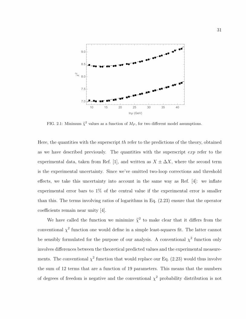
FIG. 2.1: Minimum e�2 values as a function of MF , for two di↵erent model assumptions.
Here, the quantities with the superscript th refer to the predictions of the theory, obtained
as we have described previously. The quantities with the superscript exp refer to the
experimental data, taken from Ref. [1], and written as X ± �X, where the second term
is the experimental uncertainty. Since we’ve omitted two-loop corrections and threshold
e↵ects, we take this uncertainty into account in the same way as Ref. [4]: we inflate
experimental error bars to 1% of the central value if the experimental error is smaller
than this. The terms involving ratios of logarithms in Eq. (2.23) ensure that the operator
coe�cients remain near unity [4].
We have called the function we minimize e�2 to make clear that it di↵ers from the
conventional �2 function one would define in a simple least-squares fit. The latter cannot
be sensibly formulated for the purpose of our analysis. A conventional �2 function only
involves di↵erences between the theoretical predicted values and the experimental measure-
ments. The conventional �2 function that would replace our Eq. (2.23) would thus involve
the sum of 12 terms that are a function of 19 parameters. This means that the numbers
of degrees of freedom is negative and the conventional �2 probability distribution is not
32
TABLE 2.1: Fit parameters and observables for MF = 106 GeV with �2 = 7.021. In this
example, the operator corresponding to u4 is absent from the theory. All masses are given inGeV. (Note that mt is the MS mass, not the pole mass.)
Best Fit Parameters✏ = 0.182, ✏0 = 0.005, ⇢ = 0.029, ⇠ = 0.014
defined. This reflects the fact that we could choose parameter values to set a conventional
�2 function identically to zero (i.e., there would be nothing to fit)3. Doing so, however, is
not adequate since this does not prevent a parameter value from exceeding the limits that
assure a valid e↵ective field theory. For example, a choice of parameters that gives a very
good match to all the experimental central values but includes an operator coe�cient that
3Note that there is one way that one could do a conventional �2 fit, namely, if one arbitrarily fixes asubset of the model parameters. This approach, however, is not adequate: Imagine if one fixed 14 of the19 model parameters, and fit the 12 predictions of the theory to the data in terms of the 5 free parametervalues. There are over 11, 000 di↵erent ways of choosing the set of free parameters in this example andno physical basis for choosing one set over another, nor for determining the precise values to which thefixed parameters should be set. We therefore follow an approach where all the parameters are allowed tofloat. Note that in the one case where do fix a parameter value, i.e., u4 = 0, there is a specific physicsjustification that follows from the model building considerations discussed in Sec. 3.4.
33
is, for example, 17.3, would be in wild conflict with the assumption that we have a valid
e↵ective field theory description. The e�2 function, on the other hand, includes additional
terms that give weight to the theoretical constraint that the e↵ective theory remain valid
and consistent with naive dimensional analysis. Any alternative way of imposing such a
theoretical constraint, which necessarily involves adding additional terms to the function
that is minimized that are independent of the output predictions of the theory, would not
be a conventional �2 function with the conventional statistical interpretation. Hence, we
opt for a form that is both simple and consistent with what has been used in the past
literature [4]. The quantity e�2 is useful in that it allows us to quantify the comparison
of one of our fits to another. To interpret the meaning of a given value of e�2 in absolute
terms, one then directly inspects the fit output, as we will discuss later. Since the ui, di
and `i are not treated as free parameters, we might expect qualitatively that a good fit
will have a e�2⇡ 8, corresponding to 12 pieces of experimental data minus 4 unconstrained
parameters (✏, ✏0, ⇢ and ⇠). We will see that this is consistent with our numerical results.
A plot of e�2 as a function of the flavor scale MF is shown in Fig. 2.1. The two curves
in this figure correspond to the cases were the coe�cient u4 is allowed to float, or is fixed
to zero. (In the latter case, the sum over the ui in the second line of Eq. (2.23) omits
i = 4.) These cases are motivated by two variants of the Yukawa textures that may arise
in explicit models, as we show in Sec. 3.4. Over the entire range of MF we find good fits
with e�2⇡ 8, but with clear and monotonic improvement in e�2 towards smaller values of
MF . In addition, the case where the operator corresponding to u4 is absent from the theory
(i.e., where u4 is fixed to zero), which we will see corresponds to more minimal model-
building assumptions, provides a better description of the data than the case where it is
present. We present two examples of our results in Tables 2.1 and 2.2, for MF = 106 GeV
and 1018 GeV, respectively, both in the case where u4 = 0. The first choice corresponds to
a flavor scale of the same order as the lower bounds from flavor-changing neutral current
34
TABLE 2.2: Fit parameters and observables for MF = 1018 GeV with �2 = 7.762. In this
example, the operator corresponding to u4 is absent from the theory. All masses are given inGeV. (Note that mt is the MS mass, not the pole mass.)
Best Fit Parameters✏ = 0.131, ✏0 = 0.004, ⇢ = 0.02, ⇠ = 0.011
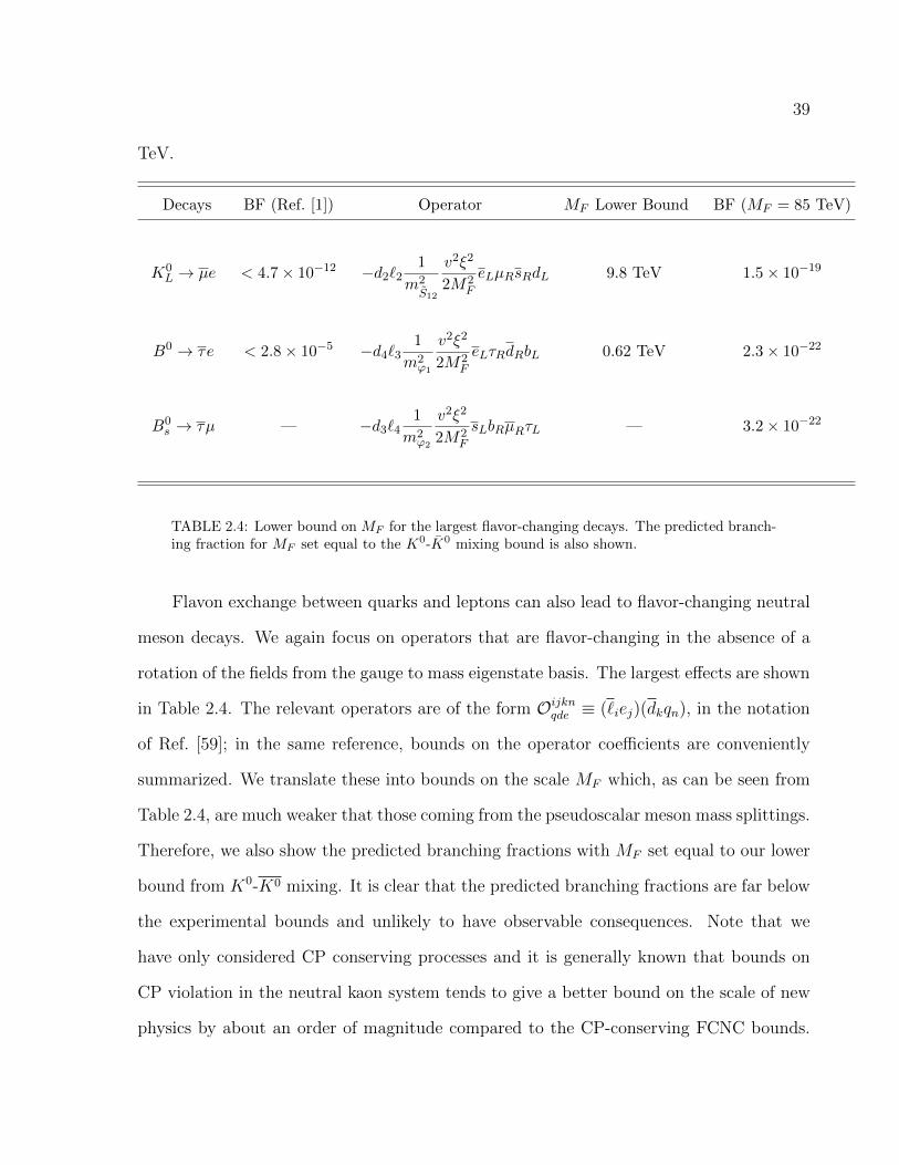
TABLE 2.4: Lower bound on MF for the largest flavor-changing decays. The predicted branch-ing fraction for MF set equal to the K
0-K0 mixing bound is also shown.
Flavon exchange between quarks and leptons can also lead to flavor-changing neutral
meson decays. We again focus on operators that are flavor-changing in the absence of a
rotation of the fields from the gauge to mass eigenstate basis. The largest e↵ects are shown
in Table 2.4. The relevant operators are of the form Oijkn
qde⌘ (`iej)(dkqn), in the notation
of Ref. [59]; in the same reference, bounds on the operator coe�cients are conveniently
summarized. We translate these into bounds on the scale MF which, as can be seen from
Table 2.4, are much weaker that those coming from the pseudoscalar meson mass splittings.
Therefore, we also show the predicted branching fractions with MF set equal to our lower
bound from K0-K0 mixing. It is clear that the predicted branching fractions are far below
the experimental bounds and unlikely to have observable consequences. Note that we
have only considered CP conserving processes and it is generally known that bounds on
CP violation in the neutral kaon system tends to give a better bound on the scale of new
physics by about an order of magnitude compared to the CP-conserving FCNC bounds.
40
Given the smallness of these branching fractions, this fact does not change our qualitative
conclusions, so we do not pursue that issue further.
2.5 Nonsupersymmetric models
In the renormalization group analysis of Sec. 2.3, the Yukawa matrices Yi are defined
by
Lm =vp2
i
LYi
i
R+ h.c. , (2.35)
where i = U , D or E and generation indices are suppressed. In order to replicate the
Yukawa textures of the supersymmetric models of Refs. [3, 4], we assign the right-handed
fermions of the three generations to the T0⇥ Z3 representations 20�
� 100. Hence, for
example, we would assign the first two generations of the charge-2/3 quarks according to
(uc
L, c
c
L) ⇠ (uR, cR) ⇠ 20�, where the superscript “c” refers to charge conjugation; since
= i cT�0�2, this is equivalent to specifying the transformation properties of the Dirac
adjoints (uL, cL). We then identify the following transformation properties for the various
blocks of the Yi,
YU,D,E ⇠
0
B@[3�
� 10�] [20+]
[20+] [100]
1
CA , (2.36)
i.e., Eq. (2.13) (or Eq. (4.1) in Ref. [4]), which omits any additional symmetries that
may be needed to explain the suppression factors ⇢ and ⇠. As in the supersymmetric
model, the transformation properties given in Eq. (2.36) determine the allowed flavon
couplings. However, in the supersymmetric case, Eq. (2.36) dictates the form of terms
in the superpotential, which is required to be a holomorphic function of the superfields.
The absence of this constraint in the nonsupersymmetric case could lead, in principle, to
additional flavon couplings that are not present in the supersymmetric theory. However,
41
we see that as far as the �, S and A flavons are concerned, this is not the case: each has a
nontrivial Z3 charge, which prevents new flavon couplings at the same order that involve
the complex conjugates of these fields.
In the supersymmetric theories of Refs. [3, 4], the additional suppression factors as-
sociated with the parameters ⇢ and ⇠ required the introduction of additional fields and
symmetries. For example, in the simplest unified T0⇥ Z3 model of Refs. [3, 4], SU(5)
charge assignments of the flavon fields are responsible for forbidding the coupling of the
A and S flavons in YU at lowest order in 1/MF . However, these couplings emerge via
higher-order operators that involve a flavor-singlet, SU(5) adjoint field ⌃ ⇠ 24, just as in
earlier models based on U(2) flavor symmetry [14]. The suppression associated with the
parameter ⇠, on the other hand, was assumed to arise via mixing in the Higgs sector, a
reasonable possibility since supersymmetric models require more than one Higgs doublet.
Here we will also achieve the additional suppression factors by means of additional
fields and symmetries. However, the additional symmetry will be much smaller than
the product of supersymmetry and a grand unified gauge group. (The latter, of course,
would not be appropriate for the non-supersymmetric case where the gauge couplings do
not unify.) We will simply assume an additional Z3 factor, so that the flavor group is
Gnew
F= T
0⇥ (Z3)
2 Defining one of the elements of the new Z3 factor as ! = exp(2 i ⇡/3),
the only standard model fields that transform nontrivially under this symmetry are
H ! !H and tR ! ! tR , (2.37)
where H is the standard model Higgs field and tR is the right-handed top quark. In the
standard model, H couples to YD and YE, while �2H
⇤ couples to YU . Hence, when the
new Z3 symmetry is unbroken, the assignments in Eq. (2.37) forbid YD and YE entirely, as
well as the first two columns of YU . How one proceeds with the model building depends
42
on the desired relative sizes of ✏, ✏0, ⇢ and ⇠. For example, for some choices of MF , it is
possible to find numerical results that are consistent with the simple possibility ✏ ⇠ ⇢ ⇠ ⇠,
up to order one factors. In this case, we assume the symmetry-breaking pattern
T0⇥ (Z3)
2 ✏�! Z
D
3✏0
�! nothing , (2.38)
where the intermediate ZD
3 factor is exactly the same one as in the original theory, that
transforms all first generation fields by a phase; in this case, the new Z3 symmetry is
broken at the first step in the symmetry-breaking chain. We introduce two new flavon
fields
⇢0 ! !2⇢0 and �! ! � , (2.39)
where � transforms like � ⇠ 20+ under the original flavor group. With the assumed
symmetry breaking pattern, the ⇢0 field and one component of the � doublet can develop
vevs of order ✏MF . The Z3 charges of these fields now allow us to rebuild our otherwise
forbidden Yukawa matrices as follows:
(i.) For YD and YE, we may generate matrices proportional to the standard form if
we replace H by H ⇢0; it follows that h⇢0i/MF is identified with the suppression factor ⇠,
which we now predict to be of order ✏, up to an order one factor. One might worry that we
could obtain a lower-order contribution from operators that don’t involve ⇢0, but involve
�⇤ instead, which also transforms under the new Z3 factor as �⇤
! !2�⇤. However, this
does not occur since �⇤⇠ 20� under the original flavor symmetry, which is not one of
the representations that leads to a lowest order coupling. On the other hand, the product
⇢⇤0� does couple at the same order as ⇢0 �; however, this additional contribution does
nothing to the form of the resulting Yukawa textures beyond a redefinition of the order
one coe�cients.
43
(ii.) For YU , the two-by-two block associated with the flavons A and S can now be
recovered via operators involving ⇢⇤0A and ⇢⇤0S. Hence, the parameter we called ⇢ previously
is now predicted to be of the same order as ⇠. In an analogous way, the 3-1 and 3-2 entries
of YU can couple to the product ⇢⇤0�, but this transforms in the same way as �, which may
couple at lower-order. Hence the canonical YU texture with an additional suppression in
only the upper-left two-by-two block is obtained. Note that we could simply omit � from
the theory and ignore the corresponding entries in YU ; this leads to an alternative texture
in which u4 = 0 in Eq. (2.13), neglecting corrections from higher-order operators. This was
the alternative possibility considered in Sec. 2.3. It is worth noting that in the case where
the � is omitted from the theory, there is no longer a necessary connection between the
scale of the additional Z3 breaking and the scale of the T 0 doublet vev, ✏MF . In this case,
we could vary this additional scale independently so that ⇢ and ⇠ are still comparable, but
intermediate in size between ✏ and ✏0. This construction would be compatible with the
numerical results in Tables 2.1 and 2.2.
In summary, we have provided an existence proof that the textures considered in our
numerical analysis may arise in a relatively simple way in a non-supersymmetric frame-
work.
2.6 Conclusions
In this chapter, we have reconsidered models of flavor based on the non-Abelian
discrete flavor group T0 that were proposed in Ref. [3, 4]. We have relaxed two assumptions
made in these studies, that the models are supersymmetric and that the scale of the flavor
sector is around the scale of supersymmetric grand unification. Our numerical study
found that T0 models without supersymmetry provide a viable description of charged
fermion masses and CKM angles for a range of values of the flavor scale MF . We find that
44
identification of MF with the reduced Planck scale is a viable possibility, consistent with a
simple picture in which no new physics appears between the weak and gravitational scales.
However, we also find that our fits improve monotonically as MF is lowered toward the
lower bound dictated by the constraints from flavor-changing-neutral-current processes. In
the case where MF is as low as possible, we identified the largest flavor-changing neutral
current e↵ects that result from the exchange of heavy flavor-sector fields; these could
provide indirect probes of the model. We then showed how the form of the Yukawa
textures that we studied, which were the same as, or closely related to, those described in
Ref. [3, 4], can nonetheless arise in a non-supersymmetric framework, where there is only a
single Higgs doublet field and where the interactions do not originate from a superpotential,
a holomorphic function of the fields. The models we described are arguably simpler than
their supersymmetric counterparts; in the non-supersymmetric case, we needed only to
extend the original flavor-group by a Z3 factor to obtain the desired Yukawa textures
shown in Eq. (2.13), while avoiding the well-known complications that come with a grand
unified Higgs sector. Extending the present study to include the neutrino sector is more
model dependent, but would be interesting for future work.
CHAPTER 3
Universal Landau Pole and Physics
below the 100 TeV Scale 1
In this chapter we reconsider the possibility that all standard model gauge couplings
blow up at a common scale in the ultraviolet. The simplest implementation of this idea
assumes supersymmetry and the addition of a single vector-like generation of matter fields
around the TeV scale. We provide an up-to-date numerical study of this scenario and
show that either the scale of the additional matter or the scale of the light superparticle
masses falls below potentially relevant LHC bounds. We then consider minimal extensions
of the extra matter sector that raise its scale above the reach of the LHC, to determine
whether there are cases that might be probed at a 100 TeV collider. We also consider
the possibility that the heavy matter sector involves new gauge groups constrained by
the same ultraviolet boundary condition, which in some cases can provide an explanation
for the multiplicity of heavy states. We comment on the relevance of this framework to
theories with dark and visible sectors.
1Work previously published in C. D. Carone, S. Chaurasia and J. C. Donahue, “Universal Landau poleand physics below the 100 TeV scale,” Phys. Rev. D 96, no. 3, 035002 (2017), [arXiv:1705.09716 [hep-ph]].
45
46
3.1 Introduction
The idea that the three gauge couplings of the standard model may assume a common
value at a high energy scale has motivated a vast literature on grand unified theories [15].
The particle content of the minimal supersymmetric standard model (MSSM) is consistent
with such a unification, with a perturbative unified gauge coupling obtained around 2 ⇥
1016 GeV. However, it was pointed out long ago [60, 61] that a di↵erent framework also
leads to the correct predictions for the gauge couplings at observable energies, namely one
in which the gauge couplings blow up at a common scale ⇤ in the ultraviolet (UV):
↵�11 (⇤) = ↵
�12 (⇤) = ↵
�13 (⇤) = 0 . (3.1)
Since the SU(3) coupling is asymptotically free, this boundary condition can only be
obtained via the introduction of extra matter [61, 62, 18, 63]. Supersymmetric models
o↵er the simplest possibility, a single vector-like generation of mass mV [61, 62, 18]. For a
chosen value of mV , one may fix the scale ⇤ by the requirement that the low-energy value
of the fine structure constant ↵EM is reproduced; the values of sin2✓W and ↵�1
3 are then
predicted at any chosen renormalization scale µ, up to theoretical uncertainties. If a value
of mV can be found in which both sin2✓W (mZ) and ↵
�13 (mZ) are consistent with the data,
then a viable solution is obtained. This approach, followed in Ref. [18], found mV around
the TeV scale, assuming that mV is also the scale of the light superparticle masses (which
we call msusy below).
A numerical renormalization group analysis cannot directly encode the boundary con-
dition in Eq. (3.1) since the gauge couplings are in the non-perturbative regime, where the
renormalization group equations (RGEs) cannot be trusted. In Ref. [18], the boundary
condition studied was ↵1(⇤) = ↵2(⇤) = ↵3(⇤) = 10, values that are barely perturbative.
47
Since the couplings are rapidly increasing as the renormalization scale is increased, one
makes the reasonable assumption that the value of ⇤ that satisfies this boundary condition
is very close to the one given by Eq. (3.1). On the other hand, as the renormalization scale
is decreased, the couplings become increasingly perturbative. Of particular importance
is that the results are insensitive to the precise choice of boundary condition as long as
each of the couplings is large [64]. It was shown in Ref. [18], that varying the ↵i(⇤) by an
order of magnitude in either direction has only a small e↵ect on the final results. We will
see this explicitly in our study of the one-vector-like-generation scenario in Sec. 3.2. The
insensitivity of the predicted values of sin2✓W (mZ) and ↵
�13 (mZ) to the choice of boundary
conditions is due to the existence of an infrared fixed point in the renormalization group
equation for the ratios of the gauge couplings [19]. Note that this insensitivity includes
the case where the ↵i(⇤) are taken to be large but not strictly identical at a common high
scale.
The possibility that the gauge couplings may have large values in the UV is interesting
from a variety of perspectives. Large couplings may arise in strongly coupled heterotic
string theories, which often also provide the additional vector-like states necessary to drive
the gauge couplings to large values [19]. On the other hand, a universal Landau pole, as
defined by Eq. (3.1), may arise in models with composite gauge bosons: compositeness
implies the vanishing of the gauge fields’ wave-function renormalization factors at the
compositeness scale, where the gauge fields become non-dynamical [65]. Redefining fields
and couplings so that the gauge fields’ kinetic terms are always kept in canonical form, one
finds that the vanishing wave-function renormalization factors translate into the blow-up
of the gauge couplings at the same scale. Thus, the framework we study may be consistent
with a wider range of possible ultraviolet completions than a conventional grand unified
theory (GUT) with a large unified gauge coupling, though it is not necessary to commit
ourselves to any one of them in order to study the consequences at low energies.
48
An additional motivation relevant to the present work is that the assumption of a
universal Landau pole leads to the expectation of new physics at a calculable energy
scale, mV , that is above the weak scale but potentially within the reach of future collider
experiments1. In Sec. 3.2, we show that the minimal scenario, involving one vector-like
generation of additional matter, requires values of either mV or msusy that are below some
of the current LHC bounds on vector-like quarks or colored superparticles, respectively.
Although experimental bounds come with model-specific assumptions that are usually easy
to evade, we pursue an alternative possibility. We show that there are small extensions of
the new matter sector that successfully reproduce the correct values of the gauge couplings
at mZ while predicting values of mV that are above the reach of the LHC, but below
100 TeV for some choices of msusy. In some cases, mV may be light enough for the vector-
like states to be explored at a 100 TeV hadron collider, which makes study of this sector
more interesting. Aside from the presence of the heavy matter fields, one possibility that
we also discuss in the present work is that these fields may transform under an additional
gauge group factor. The motivation is two-fold: (1) By placing the additional matter fields
into irreducible representations of a new gauge group, we might provide an explanation for
the multiplicity of states needed to achieve the desired UV boundary condition. In the case
where the heavy matter remains vector-like, the new gauge group can be broken at a much
lower scale. The resulting low-energy theory is that of a “dark” sector consisting of the
new gauge and symmetry breaking fields; the heavy matter provides for communication
between the dark and visible sectors, via a “portal” of higher-dimension operators that are
induced when the heavy fields are integrated out. The gauge coupling of the dark gauge
boson is predicted from a boundary condition analogous to Eq. (3.1) and the magnitude
of the portal couplings are set by the value of mV obtained in the RGE analysis. This
1This, of course, assumes that the vector-like matter occurs at a single common scale. This assumptionis relaxed in Ref. [63].
49
presents a simpler framework for constraining some of the otherwise free parameters of
a dark sector than, for example, attempting to embed both dark and visible sectors in a
conventional GUT. (2) The heavy matter may be chiral under the new gauge group. The
structure of the new sector is then more analogous to the the electroweak sector of the
MSSM, and the scale mV is associated with one or more massive gauge bosons that may
have observable consequences.
This chapter is organized as follows: In Sec. 3.2, we consider the consequences of a
universal Landau pole in the minimal case where the MSSM is augmented by a single
vector-like generation. The study presented in this section di↵ers from the past literature
not only in our use of up-to-date experimental errors for our input parameters, but also
in that we allow the scales mV and msusy to vary independently. In addition, we consider
an alternative choice for the vector-like matter that contributes the same amount to the
beta functions at one loop, but di↵ers from the one-generation scenario at two loops. In
Sec. 3.3, we consider extensions of these minimal scenarios, in particular, including a small
number of additional complete SU(5) multiplets of vector-like matter. We focus on finding
solutions in which mV is less than 100 TeV, with a special interest in cases where the
vector-like matter is light enough to be detected at a future hadron collider. In Sec. 3.4
we consider model building issues associated with the physics at the scale mV , focusing on
the implication of additional gauge groups. In Sec. 3.5, we summarize our conclusions.
3.2 One vector-like generation
In this section, we consider a minimal scenario studied in the past literature [61, 62,
18], the MSSM augmented by an additional vector-like generation of matter fields. We
denote the scale of the vector-like matter mV and we impose the same boundary conditions
as in Ref. [18], namely ↵1(⇤) = ↵2(⇤) = ↵3(⇤) = 10 as an approximation to Eq. (3.1).
50
Taking mV as an input, we determine ⇤ by the condition that the weak scale value of
the fine structure constant ↵EM(mZ) is reproduced. With ⇤ fixed, we are now able to
determine the gauge couplings at any lower scale, as a function of our choice for mV .
Above the scale msusy, we use the two-loop supersymmetric RGEs for the gauge couplings.
Below msusy, we do the same using the two-loop nonsupersymmetric RGEs, aside from
running between the top quark mass and mZ which we treat as a threshold correction
and include at one loop. We assume the presence of the second Higgs doublet required
by supersymmetry above the scale msusy. Expanding on the approach of Ref. [18], we
do not assume that the scales mV and msusy are the same, though the relaxation of that
requirement will only be important in Sec. 3.3.
As indicated in the introduction, the ratios of the gauge couplings are driven towards
infrared fixed point values, so that predictions for sin2 ✓W and ↵�13 at mZ are relatively
insensitive to the choice of boundary conditions at the scale ⇤. For example, allowing the
↵i(⇤) to vary independently between 1 and 100, we find that the their weak-scale values
scatter within roughly 2% for ↵1(mZ) and ↵2(mZ) and 5% for ↵3(mZ). Given the same
variation of boundary conditions, we take the resulting scatter in the values of sin2✓W (mZ)
and ↵�13 (mZ) as a measure of the theoretical uncertainty in our output predictions. We
include these estimates with our numerical results.
The RGEs that we use above the top mass have the form
dgi
dt=
gi
16⇡2
"big
2i+
1
16⇡2
3X
j=1
bijg2ig2j�
X
j=U,D,E
aijg2iTr[YjY
†j]
!#, (3.2)
where t = lnµ is the log of the renormalization scale, ↵i = g2i/4⇡, and the Yi are Yukawa
matrices. The beta function coe�cients bi and bij can be determined using general formu-
lae [67, 68]. For example, in the case of one vector-like generation with mV = msusy, one
51
finds for µ > mV
bi =
0
BBBB@
53
5
5
1
1
CCCCAand bij =
0
BBBB@
977
75
39
5
88
313
553 40
11
315
178
3
1
CCCCA, (3.3)
while for mt < µ < mV we have the nonsupersymmetric beta functions
bNS
i=
0
BBBB@
41
10
�19
6
�7
1
CCCCAand b
NS
ij=
0
BBBB@
199
50
27
10
44
59
10
35
612
11
10
9
2�26
1
CCCCA. (3.4)
More general forms for the one- and two-loop beta functions that take into account the
possibility of additional matter are presented in Sec. 3.3. Note that the gauge couplings
for µ > msusy are defined in the dimensional reduction (DR) scheme, which preserves
supersymmetry; the couplings are converted to the modified minimal subtraction scheme
(MS) at the matching scale µ = msusy before they are run to lower energies. The gauge
couplings in the two schemes are related by [69]
4⇡
↵MSi
=4⇡
↵DRi
+1
3(CA)i , (3.5)
where CA = {0, 2, 3} for i = 1, 2, 3.
The coe�cients for the terms that depend on the Yukawa couplings in Eq. (3.2) are
given by
aij =
0
BBBB@
265
145
185
6 6 2
4 4 0
1
CCCCAand a
NS
ij=
0
BBBB@
1710
12
32
32
32
12
2 2 0
1
CCCCA, (3.6)
52
for µ > msusy and µ < msusy, respectively. In practice, we only need to take the top quark
Yukawa coupling yt into account, since it is significantly larger than the other Yukawa
couplings. Since yt a↵ects the running of the gauge couplings only through a two-loop
term, we need only include its running at one-loop. For µ > msusy we have [54]
dyt
dt=
yt
16⇡2
⇣�
Xcig
2i+ 6y2
t
⌘, ci =
✓13
15, 3,
16
3
◆, (3.7)
while for µ < msusy [54],
dyt
dt=
yt
16⇡2
✓�
XcSMi
g2i+
9
2y2t
◆, c
SMi
=
✓17
20,9
4, 8
◆. (3.8)
For definiteness, we assume tan � = 2, and compute the weak scale value of yt via yt(mZ) =p2mt
v sin �, using the MS value of the top quark mass, 160+5
�4 GeV [1], and v = 246 GeV. The
value yt(⇤) is computed numerically so that we obtain the desired yt(mZ) value for a given
set of input parameters. While this approach is su�cient to determine the representative
impact of including the top quark Yukawa coupling in our RGE analysis, it turns out to be
overkill: in models where the gauge couplings blow up in the UV, the top quark Yukawa
coupling is rapidly driven to zero in the same limit. Hence, its e↵ect on the values of mV
and ⇤ determined in our numerical analysis turns out to be small, less than the estimates
of theoretical uncertainty that we build into the analysis. Although we include it, ignoring
yt altogether does not a↵ect our results qualitatively and can be a useful approach for
speeding up numerical cross-checks.
For a given choice of mV and msusy, the blow-up scale ⇤ is chosen to yield the correct
value of the fine structure constant at the weak scale,
↵�1EM(mZ) =
5
3↵�11 (mZ) + ↵
�12 (mZ), (3.9)
53
where the factor of 5/3 comes from the fact that we assume SU(5) normalization [55] of
the U(1) gauge coupling, as in Ref. [18]. While this makes the analysis compatible with
a conventional SU(5) GUT at large coupling, this normalization can also arise directly in
string theory without an SU(5) GUT [66]. Other normalizations of the U(1) factor are
certainly possible, depending on the UV completion. However, we do not consider other
possibilities here and adopt the normalization that has been assumed almost uniformly in
the past literature. For our numerical study, we take the target central value of ↵�1EM(mZ) =
127.95 [1]. With ⇤ determined in this way, we compute ↵3(mZ)�1 and the Weinberg angle
sin2✓W (mZ), which is determined by ↵1(mZ) and ↵2(mZ):
sin2✓W (mZ) =
3↵1(mZ)
3↵1(mZ) + 5↵2(mZ). (3.10)
We compare the output predictions of ↵3(mZ)�1 and sin2
✓W (mZ), including the theoretical
uncertainty that we discussed earlier, to the experimentally measured values [1]
sin2✓W = 0.23129± 5⇥ 10�5
, ↵�13 (mZ) = 8.4674± 0.0789 , (3.11)
both given in the MS scheme. A previous study of the one vector-like generation scenario
found viable solutions with mV = msusy ⇡ 1 TeV [18]. Since the time of that work, the ex-
perimental errors in sin2✓W (mZ) and ↵
�13 (mZ) have decreased substantially. Nevertheless,
as indicated in Table 3.1, we find mV = msusy ⇡ 1.2 TeV, assuming ±2 standard deviation
experimental error bands and using our protocol for determining theoretical error bands;
those bands are both displayed in Fig. 3.1. To determine the theoretical error band, we
find the maximum and minimum values of sin2✓W (mZ) and ↵
�13 (mZ) that are obtained by
varying the ↵i independently between 1 and 100 at the blow-up scale. In particular, we find
that sin2✓W (mZ) is maximum when {↵1(⇤), ↵2(⇤), ↵3(⇤)} = {100, 1, 100} and minimum
54
0.22
0.225
0.23
0.235
0.24
0.245
0.25
0.255
0.26
0.1 1 10
msusy
= mV
exp.
mV
mV
mV
sin2 θ
W (m
Z)
7
8
9
10
11
12
0.1 1 10
α3-1
(mZ)
mV
msusy
= mV
exp.
mV
FIG. 3.1: The dependence of sin2 ✓W (mZ) and ↵�13 (mZ) on the mass of the vector-like gen-
eration, mV , including theoretical uncertainties. In this example, the light superparticle massscale msusy is identified with mV . The acceptable ranges of mV in each of the plots havenon-vanishing overlap for 1.15 TeV< mV < 1.31 TeV, indicating a viable solution.
when the boundary condition set is {1, 100, 1}; ↵�13 (mZ) is maximized and minimized for
the sets {100, 100, 1} and {1, 1, 100}, respectively. We quote the variation in the out-
put predictions as a percentage relative to the value obtained when the ↵i(⇤) = 10, for
i = 1 . . . 3, in Table 3.1. For the values of mV that yield viable predictions for sin2✓W (mZ)
and ↵�13 (mZ), we find that the scale ⇤ is around 8⇥ 1016 GeV.
Model mSUSY (TeV) mV range (TeV) ⇤ range (GeV) ↵�13 (mZ) % error sin2 ✓W (mZ) % error
TABLE 3.1: Numerical results formV and ⇤ in the one-generation scenario, the (5,2,0,0) model,and a model whose vector-like sector consists of four 5 + 5 pairs, the (3,2,4,0) model. Thesemodels have the same one-loop beta functions, but di↵er at two-loop. Also shown are thetheoretical error estimates as discussed in the text.
The value of msusy for this solution can be compared to recent bounds on gluinos
from the LHC, which now exceed 2 TeV (for example, see Ref. [70]). These bounds
generally make assumptions about the supersymmetric particle spectrum (for example,
light neutralinos) and one can always play the game of making model-specific adjustments
to evade the assumptions of any given experimental exclusion limit. We will not pursue that
55
approach here. We instead consider the possibility that mV and msusy are not identical, so
that msusy can be raised unambiguously above the LHC reach. In this case, however, we
obtain lower values of mV , which in this model would place an entire vector-like generation
below 1 TeV. As a point of comparison, current LHC bounds on a charge-2/3 vector-like
quark that decays 100% of the time to bW is 1.295 TeV at the 95% CL [71]. The same
comment regarding the limitations of experimental exclusion limits applies here as well;
we will be content simply to point out that the one-generation model will become less
plausible as time goes on given the increasing reach of LHC searches for superparticles
and vector-like quarks.2
This result motivates the topic of the next section, extensions of this minimal sector
that include sets of new particles that fill complete SU(5) multiplets. We find that these
lead to larger values of mV . In studies of perturbative gauge coupling unification, it is well
known that adding additional matter in complete SU(5) multiplets preserves successful
unification. In the present framework, we find viable solutions for mV are also obtained
when complete SU(5) multiplets are added. To study the e↵ect on mV and ⇤, we consider
adding the smallest SU(5) representations, with dimensions five and ten, allowing for
multiple copies. We label models by four numbers (ng, nh, n5, n10) which represent the
number of chiral generations, complex Higgs doublets, 5+ 5 pairs and 10+ 10 pairs.3 In
this notation, the one-vector-like-generation scenario that we have discussed in this section
will be called the (5, 2, 0, 0) model henceforth. We note that a model with four 5+ 5 pairs
added to the MSSM, the (3, 2, 4, 0) model, has the same one-loop beta functions as the
(5, 2, 0, 0) model, and could be considered an equally minimal alternative. Results for
the (3, 2, 4, 0) model are also shown in Table 3.1, and are useful for illustrating the e↵ect
2Unless, of course, some of these particles are discovered.3It is interesting to note that in level-one string theories with Wilson line symmetry breaking, extra
vector-like matter will naturally appear in 5+ 5 and 10+ 10 pairs, since these are representations foundin the 27+ 27 of E6 [19].
56
of di↵erent two-loop beta functions. The preferred range of mV in the (3, 2, 4, 0) model
is slightly below that of the (5, 2, 0, 0) model, again pointing to the need for alternative
choices for the new matter sector to avoid potential phenomenological di�culties.
3.3 Next-to-minimal possibilities
In this section, we consider vector-like matter sectors that are consistent with values
of the superparticle masses and mV that are no smaller than 2 TeV. We look at next-
to-minimal scenarios, i.e. ones with a small number of additional 5 + 5 and 10 + 10
pairs, for the reasons discussed at the end of the previous section. We have particular
interest in solutions that may be plausible for exploration at a 100 TeV hadron collider.
To proceed, we use the results for the one- and two-loop beta functions, derived from the
general formulae in Refs. [67] and [68]. In the supersymmetric case, we find
bi =
0
BBBB@
2
2
2
1
CCCCAng +
0
BBBB@
310
12
0
1
CCCCAnh +
0
BBBB@
1
1
1
1
CCCCAn5 +
0
BBBB@
3
3
3
1
CCCCAn10 +
0
BBBB@
0
�6
�9
1
CCCCA, (3.12)
bij =
0
BBBB@
3815
65
8815
25 14 8
1115 3 68
3
1
CCCCAng +
0
BBBB@
950
910 0
310
72 0
0 0 0
1
CCCCAnh
+
0
BBBB@
2145
95
3215
35 7 0
415 0 34
3
1
CCCCAn5 +
0
BBBB@
235
35
485
15 21 16
65 6 34
1
CCCCAn10 +
0
BBBB@
0 0 0
0 �24 0
0 0 �54
1
CCCCA, (3.13)
57
while in the nonsupersymmetric case,
bNS
i=
0
BBBB@
43
43
43
1
CCCCAng +
0
BBBB@
110
16
0
1
CCCCAnh +
0
BBBB@
23
23
23
1
CCCCAn5 +
0
BBBB@
2
2
2
1
CCCCAn10 +
0
BBBB@
0
�223
�11
1
CCCCA, (3.14)
bNS
ij=
0
BBBB@
1915
35
4415
15
493 4
1130
32
763
1
CCCCAng +
0
BBBB@
950
910 0
310
1316 0
0 0 0
1
CCCCAnh +
0
BBBB@
730
910
1615
310
496 0
215 0 38
3
1
CCCCAn5
+
0
BBBB@
2310
310
245
110
492 8
35 3 38
1
CCCCAn10 +
0
BBBB@
0 0 0
0 �1363 0
0 0 �102
1
CCCCA. (3.15)
As indicated earlier, ng, nh, n5 and n10 represent the number of chiral generations, Higgs
doublets, 5+ 5 and 10+ 10 pairs, respectively. One can check that these formulae reduce
to the expected results for the MSSM, where ng = 3, nh = 2, n5 = n10 = 0 in Eqs. (3.12)
and (3.13), and for the standard model, where ng = 3, nh = 1, n5 = n10 = 0 in Eqs. (3.14)
and (3.15).
Table 3.2 displays results analogous to those presented for the minimal scenario in
Table 3.1, for a variety of heavy matter sectors, withmsusy mV . The cases considered fall
into pairs that have the same one-loop beta functions; for example, adding one additional
5 + 5 pair to the one-vector-like generation scenario gives us the (5, 2, 1, 0) model, which
has the same bi as a model with five 5 + 5 pairs, namely (3, 2, 5, 0). The same can be
said for the remaining two models, involving six 5+5 and two 10+10 pairs, respectively.
Results are shown for values of msusy ranging from 2 TeV to mV . We see that solutions
58
Model mSUSY (TeV) mV range (TeV) ⇤ range (GeV) ↵�13 (mZ) % error sin2 ✓W (mZ) % error
TABLE 3.3: Solutions for mV and ⇤ for msusy > mV . Here mV refers to the fermionic com-ponents of the vector-like sector, while msusy represents a common mass for the superparticlesof the ordinary and vector-like sectors. Of the models in Table 3.2, only the (3, 2, 0, 2) caseprovides viable solutions.
collider experiments, particularly in the case where the superparticle mass scale exceeds
the scale mV . Aside from the extra matter fields, other physics associated with this sector
might also be experimentally probed. In this section, we consider two motivations for
including an extra gauge group that only a↵ects the heavy fields:4 (1) The heavy fields
may fall in irreducible representations of the new gauge group, explaining the multiplicity
of new particles required to achieve the blow up of the couplings at the scale ⇤, and (2)
the new sector may be chiral under the new gauge groups, rendering it more analogous in
structure to the matter sector of the MSSM. Although there are a large number of ways in
which either possibility might arise, we consider one example here, based on the (3, 2, 0, 2)
model discussed in the previous section.
Regarding the first motivation, we consider the possibility that the duplication of
vector-like 10+ 10 pairs in the (3, 2, 0, 2) model is a result of their embedding into a two-
dimensional representation of an additional gauge group, which is necessarily non-Abelian.
The simplest possibility for the gauge group structure of the model is GSM⇥SU(2)X , where
GSM represents the standard model gauge factors. As before, we indicate the standard
model charge assignments implicitly and compactly by displaying the SU(5) multiplets
that the heavy matter fields would occupy in a conventional unified theory, even though
that is not our assumption. Hence under SU(5)⇥SU(2)X , we now assume that the extra
4In the context of strong unification, extensions of the standard model gauge group have been consideredfor other purposes in Ref. [75].
61
matter is given by
⇠ (10, 2) and ⇠ (10, 2) . (3.16)
We also introduce two SU(2)X doublet Higgs fields that will be responsible for sponta-
neously breaking the new gauge group factor
�1 ⇠ (1, 2) and �2 ⇠ (1, 2) . (3.17)
The matter fields in Eq. (3.16) and the new Higgs fields in Eq. (3.17) are separately vector-
like, so that these fields may be made massive at any desired scale; it also follows that
all chiral gauge anomalies are canceled. Note that the multiplicity of SU(2) doublets in
Eqs. (3.16) and (3.17) is even, which implies that the SU(2)X Witten anomaly is absent.
Given these assignments, the one-loop beta function for the new gauge factor is positive,
allowing for straightforward implementation of the UV boundary condition in Eq. (3.1).
One issue that needs to be addressed in a model like this one is the stability of the
extra matter fields. Vector-like 5+ 5 and 10+ 10 pairs have the appropriate electroweak
and color quantum numbers to participate in mass mixing with standard model matter
fields. The amount of such mixing is arbitrary, and only a small amount is necessary
so that the heavy states are rendered unstable, avoiding any cosmological complications.
Assigning the matter fields of the heavy sector to multiplets of a new gauge group can
have unwanted consequences if these states are rendered exactly stable (or extremely long
lived). In the present model, this problem does not arise provided that the new gauge
group is spontaneously broken, since mass mixing is generated via renormalizable couplings
involving , the �i, and the standard model fields identified with a 10. If embedding in
an additional gauge group is used to account for the multiplicity of states in some of the
other models that we have considered, the model must also provide for the decay of the
62
heavy states; the (3, 2, 0, 2) models seem to naturally avoid this problem with smallest
field content and the potentially simplest symmetry-breaking sector, which is one reason
why we focus on this example here.
Note that the numerical results for the (3, 2, 0, 2) model described in Sec. 3.3 must
be adjusted to take into account the presence of the SU(2)X gauge group, whose coupling
blows up at the same scale as the other gauge couplings and a↵ects their renormalization
group running. However, since the e↵ect is only via two-loop terms, we don’t expect a
dramatic change in our qualitative conclusions. To support this statement, we consider
the case where msusy = mV and take into account the e↵ect of the new gauge group by
modifying the supersymmetric RGEs for running between the scales ⇤ and mV . In this
case, the supersymmetric beta functions become
bi =
✓63
57 3 5
◆, (3.18)
bij =
0
BBBBBBBB@
429
25
33
5
184
518
11
567 56 18
23
521 82 18
6 18 48 53
1
CCCCCCCCA
. (3.19)
Repeating the analysis of Sec. 3.3, we find only a modest adjustment in the ranges for mV
and ⇤, as shown in Table 3.4 below.
Model mSUSY (TeV) mV range (TeV) ⇤ range (GeV) ↵�13 (mZ) % error sin2 ✓W (mZ) % error
TABLE 3.4: Results for the (3, 2, 0, 2) scenario with mV = msusy taking into account the e↵ectof the SU(2)X gauge group.
It is interesting to note that SU(2)X breaking scale is not tied to the value ofmV in this
model, which means it could in principal be much lower. For example, with h�i ⇠ 1 GeV,
63
the resulting low-energy e↵ective theory would be that of a non-Abelian dark sector with a
one- or two-Higgs doublet symmetry-breaking sector. Communication between the visible
and dark sectors would follow from operators generated when the mV -scale physics is
integrated out, suggesting that this sector may have other interesting consequences besides
its e↵ect on gauge coupling running. Whether phenomenologically interesting models of
this type can be constructed remains an open question.
Finally, we note that a di↵erent motivation for an extra gauge factor is to render the
mV -scale physics chiral, so that the structure of the new matter sector is more similar
to the rest of the MSSM. In the previous example, we could simply change the charge
assignment of to
1 ⇠ (10, 1) and 2 ⇠ (10, 1) . (3.20)
Now the mass terms for the extra matter are generated via Yukawa couplings involving
, and the �i; the vacuum expectation value h�i is now associated with the scale mV
determined in the RGE analysis. We make one additional modification to the theory,
which is to add an additional pair of Higgs fields
�01 ⇠ (1, 2) and �
02 ⇠ (1, 2) . (3.21)
The modification in Eq. (3.20) leads to the vanishing of the one-loop beta function for
SU(2)X , while Eq. (3.21) restores the desired asymptotic non-freedom. Based on our
earlier observations, it is clear that the numerical values for mV and ⇤ in this model will
be qualitatively similar to those of the other (3, 2, 0, 2) models that we have considered,
and we leave further numerical study for the interested reader.
64
3.5 Conclusions
In this chapter, we have revisited the possibility that the standard model gauge cou-
plings reach a common Landau pole in the ultraviolet. This provides a predictive frame-
work for relating the values of the gauge couplings at the weak scale, without the necessary
assumption of conventional grand unification. To implement this framework, all the gauge
couplings must be asymptotically non-free, which implies that new matter must be in-
cluded in the theory. We have numerically explored the possibility that this new matter
appears at two scales, a light superpartner mass scale msusy, and the scale where addi-
tional heavier vector-like states appear, mV . We have revisited a scenario considered in
the past in which the minimal supersymmetric standard model is enlarged by a single
vector-like generation and found that either msusy or mV falls below potentially relevant
LHC lower bounds on colored MSSM superparticles or vector-like quarks. Although one
cannot rule out the possibility that these states are present and have evaded detection
for model-specific reasons, we are motivated to consider a safer possibility: we include a
relatively small additional amount of extra heavy matter, which leads to solutions for mV
that are beyond the reach of the LHC, but potentially within the reach of a higher-energy
hadron collider. For example, given a heavy sector consisting in total of five 5 + 5 pairs,
we obtain successful gauge coupling predictions for msusy = mV ⇡ 13 TeV. For a heavy
sector of two 10+10 pairs, we can achieve mV as low as 3 TeV, if we allow higher values of
msusy ⇡ 1500 TeV. (In this case, mV refers to the fermionic components of the vector-like
sector, while msusy represents a common mass for the superparticles of the ordinary and
vector-like sectors.)
We also considered whether the size of the new matter sector could be related to its
embedding into the irreducible representation of an additional non-Abelian gauge group.
We presented the simplest model that was consistent with our numerical solutions, a
65
model with two 10+ 10 pairs, in which this duplication is due to their embedding in the
fundamental representation of a new SU(2) gauge group. In the case where the heavy
matter sector is vector-like under the new SU(2), the new gauge group can be broken at
a much lower scale and the e↵ective theory is that of a spontaneously broken non-Abelian
dark sector. In the case where the heavy matter sector is chiral under the new SU(2),
mV is associated with the symmetry breaking scale. In this case, new heavy gauge bosons
would be among the spectrum of particles that might be sought at a future collider with
a suitable reach.
CHAPTER 4
Curved Backgrounds in Emergent
Gravity 1
Field theories that are generally covariant but nongravitational at tree level typically
give rise to an emergent gravitational interaction whose strength depends on a physical
regulator. In this chapter we consider emergent gravity models in which scalar fields
assume the role of clock and rulers, addressing the problem of time in quantum gravity.
We discuss the possibility of nontrivial dynamics for clock and ruler fields, and describe
some of the consequences of those dynamics for the emergent gravitational theory.
1Work previously published in S. Chaurasia, J. Erlich and Y. Zhou, “Curved Backgrounds in EmergentGravity,” Class. Quant. Grav. 35, no. 11, 115008 (2018), [arXiv:1710.07262 [hep-th]].
66
67
4.1 Introduction
The possibility that gravitation emerges from other interactions provides a promising
paradigm for addressing the di�cult conceptual questions that confront quantum gravity.
These questions include the problem of time, namely that coordinate invariance implies a
vanishing Hamiltonian and the consequent absence of dynamics of quantum states [76]; the
question of predictivity in a theory with nonrenormalizable interactions such as gravitation;
the question of what observables are physical in a di↵eomorphism-invariant theory; and
questions related to the vacuum, including why the Minkowski spacetime and its signature
should be preferred to other spacetimes in a quantum theory in which spacetime geometries
are integrated over.
The possibility of emergent long-range interactions in quantum field theory has been
recognized for half a century.1 Bjorken argued that four-fermi models with current-current
interactions can give rise to emergent gauge interactions [22], and Eguchi later argued that
the composite gauge field in such theories may render those theories renormalizable despite
the presence of fundamental four-fermi interactions [23]. It did not take long for the idea
of emergent interactions to be extended to gravitation, in a wonderfully short note by
Sakharov [26]. Sakharov pointed out that the regularized e↵ective action for the spacetime
metric generically contains the Einstein-Hilbert term even if no such term is present at
tree level, as long as general covariance is maintained by the regulator in the theory. This
suggests that the dynamics of spacetime might emerge as an artifact of regulator-scale
physics even if there is no such dynamics prior to quantization.2
Perhaps the most compelling argument for emergent gravity is its ubiquity: all that
1In a classical context, Michael Faraday suspected a relationship between electromagnetism and grav-itation, and in the 1840s searched experimentally for such an identification. He was unsuccessful [77].
2Sakharov had in mind that the spacetime metric was to be treated classically, in which case theinduced gravity is semiclassical, with the vacuum expectation value of the energy-momentum tensor Tµ⌫
being related to the spacetime metric by Einstein’s equations (with cosmological constant, plus regulator-suppressed corrections).
68
is needed is a generally covariant description of the interactions of a field theory and
a covariant regulator that resolves infinities in perturbation theory, both of which are
likely to be required of quantum gravity, in any case. Much work has been done in an
attempt to turn Sakharov’s observation into a compelling description of quantum gravity
[78, 79, 80, 81], but certain di�culties remain. More recently, alternative paradigms that
also appear to lead to emergent gravitational interactions have gained favor, such as the
AdS/CFT correspondence [82], entropic gravity [83], and emergent spacetime via networks
of entangled states [84, 85]. However, the present work concerns the old-fashioned approach
to the subject as motivated by Sakharov’s induced gravity.
The problem of nonrenormalizability of the gravitational interaction persists in emer-
gent gravity, unless the quantum theory is asymptotically safe by virtue of an ultraviolet
fixed point [86]. However, with the presumption of a physical regulator, the lack of predic-
tivity of the theory is augmented by the more fundamental ontological question of what is
to be demanded of the theory at short distances. Regulators in quantum field theory have
the habit of violating some cherished principle or another, such as unitarity or boundedness
of the Hamiltonian from below. In the present work we are agnostic about the physical
regulator and its consequences for the interpretation of the theory at short-distances, and
we require only that the theory provide a definite rule for calculating correlation functions
of appropriate observables at all physical scales. For the purpose of illustration we will use
dimensional regularization, fixing the spacetime dimension D by holding ✏ = D � 4 small
but fixed.
The problem of time demands that physical degrees of freedom playing the roles of
clock and rulers be identified in any generally covariant theory. This allows dynamics to
be interpreted in terms of correlations, or entanglement [87], between physical degrees
of freedom and the clock and rulers. For example, certain scalar fields XJ(xµ) can play
the role of the physical clock and rulers by a gauge-fixing condition analogous to the
69
static-gauge condition in string theory, under the presumption that field configurations
dominating the functional integral can be put into that gauge. Here xµ are the spacetime
parameters integrated over in the action, and the indices J and µ both take values in
{0, ..., D � 1}. The gauge choice is XJ = c xµ�J
µfor some constant c that will be specified
for convenience later. In the models considered here, this choice for the fieldsXJ satisfy the
classical equations of motion with all other fields sitting at the minimum of the potential,
and there is a natural perturbative expansion about this classical background.
In this chapter we generalize a particular toy model of emergent gravity that was
recently studied in Ref. [27]. The model contains only scalar fields, and D of the fields
play the role of clock and rulers in D dimensions. The model was shown to include a
massless composite graviton in its spectrum which couples at leading order to the energy-
momentum tensor of the physical (non-gauge-fixed) fields as in Einstein gravity. The
model is generally covariant from the outset, has a vanishing energy-momentum tensor
(including the contributions of the clock and ruler fields), and thereby evades the Weinberg-
Witten no-go theorem which prohibits the existence of massless spin-2 particles in a broad
class of Lorentz-invariant theories [88]. Di↵eomorphism invariance is expected to lead to
gravitational self-interactions beyond leading order consistent with general relativity up to
Planck-suppressed corrections, and evidence for this by direct computation was recently
provided in Ref. [89]. Here we generalize the theory to the case in which the clock and
ruler fields have a nontrivial field-space metric, and we demonstrate that, at leading order
in a perturbative expansion, scattering is as in Einstein gravity in a spacetime background
identified with the field-space metric.
70
4.2 Emergent Gravity with Curved Backgrounds
The theory that we study includes N scalar fields �a, a 2 {1, . . . , N}, in addition to
the D scalar fields XJ that play the role of clocks and rulers. We assume the potential
depends only on �a but not the clock and ruler fields. The theory is defined so as to
be di↵eomorphism invariant, and at the classical level the theory is independent of any
geometric structure imposed on the spacetime other than di↵erentiability. In particular,
the action is independent of spacetime metric on the coordinates xµ, and correspondingly
the theory has an identically vanishing energy-momentum tensor. The action for the
theory is,
S =
ZdD
x
D
2 � 1
V (�a)
!D2 �1
vuut�����det
NX
a=1
@µ�a @⌫�
a +D�1X
I,J=0
@µXI @⌫X
J GIJ(XK)
!�����. (4.1)
Aside from the dependence of the action on a potential V (�a), this theory is in the class
of induced gravity theories based on the Nambu-Goto-like membrane action, as analyzed
recently in Ref. [90].
The theory described by Eq. (4.1) is nonlinear, but it is reminiscent of the Nambu-Goto
action for the string and we can motivate it by introducing an auxiliary spacetime metric
which is fixed by a constraint of vanishing energy-momentum tensor. The Polyakov-like
description of the theory is given by the action,
S =
ZdD
x
p|g|
"1
2gµ⌫
NX
a=1
@µ�a@⌫�
a +D�1X
I,J=0
@µXI@⌫X
JGIJ(X
K)
!� V (�a)
#. (4.2)
The quantum theory is defined by functional integral quantization over the scalar fields
and gµ⌫(x), subject to the constraint Tµ⌫ = 0. The constraint can be thought of as arising
from integrating out the auxiliary-field metric gµ⌫ , although in that case a Jacobian func-
71
tional determinant would also arise from the functional integration, which would appear
to modify the theory nonperturbatively. (An analogy to this in the context of a model
of emergent gauge interactions was pointed out in Ref. [91].) Nonetheless, as long as the
action, constraints and regulator are covariant, an emergent gravitational interaction can
be expected as in Sakharov’s induced gravity.
The partition function for the theory is,
Z =
Z
Tµ⌫=0
Dgµ⌫ D�aDX
IeiS(�a,XI
,gµ⌫), (4.3)
where the symmetric energy-momentum tensor is defined in the usual way,
Tµ⌫(x) =2p|g|
�S
�gµ⌫(x)(4.4)
=NX
a=1
@µ�a@⌫�
a +D�1X
I,J=0
@µXI@⌫X
JGIJ � gµ⌫L, (4.5)
where the Lagrangian L is defined by the action in Eq. (4.2), S ⌘
ZdD
x
p|g|L. Eq. (4.5)
is solved by
gµ⌫ =D/2� 1
V (�a)
NX
a=1
@µ�a@⌫�
a +D�1X
I,J=0
@µXI@⌫X
JGIJ
!, (4.6)
which together with Eq. (4.2) gives the membrane-like action Eq. (4.1). Note that gµ⌫ of
Eq. (4.6) is auxiliary and does not have dynamics other than that due to its dependence
on the fields �a and XI . Also note that, despite the similarity of the actions Eq. (4.1) and
Eq. (4.2) to the Nambu-Goto and Polyakov actions of string theory, the factor of D/2� 1
in Eq. (4.6) hints that the case D = 2 is special. In D = 2, a conformal factor rescaling
the metric of Eq. (4.6) factors out of the equations of motion and allows for the transition
from the Polyakov form to the Nambu-Goto form of the string action.
We assume that the potential V (�) has the form V (�) = V0 + �V (�), with the
72
minimum of the potential V0 much larger than any other scales in the theory with the
possible exception of a scale associated with the physical regulator. For simplicity we
also assume in our analysis that the field-space metric GIJ(XK) ⌘ ⌘IJ + eHIJ(X
K), with
Minkowski (mostly-minus) metric ⌘IJ , admits a perturbative expansion in eHIJ and its
derivatives.
The theory described by Eq. (4.1) is invariant under coordinate reparametrizations,
XI(x) ! X
I(x0(x)) and �a(x) ! �
a(x0(x)); and under field redefinitions the field-space
metric GIJ transforms like a metric: If XI(x) is replaced with X0 I(XJ(x)) and GIJ(X) is
replaced with G0IJ(X 0),
@µXI@⌫X
JGIJ(X) ! @µX
0 I@⌫X
0 JG
0IJ(X 0)
= @µXK@⌫X
L@X
0 I
@XK
@X0 J
@XLG
0IJ(X 0(X)) (4.7)
= @µXI@⌫X
JGIJ(X),
where the last line follows if
G0IJ(X) =
@XK
@X 0I@X
L
@X 0J GKL(X0(X)). (4.8)
Note that a field redefinition cannot take a curved-space GIJ to a flat-space one, so the the-
ory with generic field-space metric is genuinely inequivalent to the flat-field-space version
of the theory studied previously.
In order to provide physical meaning to the spacetime background in which dynamics
take place, we identify XI with the corresponding spacetime coordinates (up to a constant
factor), analogous to a static gauge condition in string theory:
XI =
sV0
D/2� 1xµ�I
µ, I = 0, . . . , D � 1, (4.9)
73
Then the field X0 can be interpreted as an internal clock [87], while the fields X
i, i =
1, . . . , D � 1 are interpreted as rulers. In this case the Fadeev-Popov determinant is
det
✓�X
I,↵ (y)
�↵µ (y0)
◆= det
sV0
D
2 � 1
� (yµ + ↵µ (y))
�↵µ (y0)�I
µ
!
= det
sV0
D
2 � 1�I
µ�(D) (y � y
0)
!,
(4.10)
which is trivial and consequently there are no Fadeev-Popov ghosts resulting from gauge
fixing XI .
The classical equations of motion for �a and XI following from the action Eq. (4.2)
are
1p�g
@µ
�p�gg
µ⌫@⌫�
a�= �
@V
@�a, (4.11)
@µ
�p�gg
µ⌫GIJ@⌫X
J�=
1
2
p�gg
µ⌫@µX
J@⌫X
K@
@XIGJK . (4.12)
If we set �a = �a
min where �a
min minimizes V such that V (�a
min) = V0, then the equation of
motion for �a is trivially satisfied. Meanwhile, with the gauge-fixed background XI as in
Eq. (4.9), the spacetime metric at �a = �a
min is
gµ⌫ =D
2 � 1
V0
�pV0�
I
µ
� �pV0�
J
⌫
�GIJ
D
2 � 1= Gµ⌫(x
I), (4.13)
so the spacetime background in which the fields �a propagate is now identified with the
field-space metric for the clock and ruler fields. Furthermore, the equations of motion for
the clock and ruler fields, Eq. (4.12), are also satisfied by the static gauge condition, as is
readily checked using the identity,
1p|g|
@
p|g|
@x↵=
1
2gµ⌫@gµ⌫
@x↵. (4.14)
74
Hence, the static-gauge configuration with fields �a uniform at the minimum of the po-
tential, and with gµ⌫(x) = Gµ⌫(x), solve the equations of motion and provide a classical
background about which the dynamics for the fields �a can now be analyzed.
We now show that the background GIJ modifies the emergent gravitational interaction
by coupling to the matter fields as in Einstein gravity, at linear order in the expansion
about the Minkowski metric. Thus we write the background GIJ as,
Gµ⌫ = g(B)µ⌫
= ⌘µ⌫ + eHµ⌫ , (4.15)
where eHµ⌫ determines the background spacetime but is assumed to be small compared to
⌘µ⌫ . Consequently the gauge-fixed action takes the form,
S =
ZdD
xV0
D/2� 1
✓V0
V0 +�V (�a)
◆D/2�1r���det⇣⌘µ⌫ + eHµ⌫ + ehµ⌫
⌘���, (4.16)
where
ehµ⌫ ⌘D/2� 1
V0
NX
a=1
@µ�a@⌫�
a
!, (4.17)
and gµ⌫ depends on the field configuration via,
gµ⌫ =V0
V (�)
⇣⌘µ⌫ + eHµ⌫ + ehµ⌫
⌘. (4.18)
In order to analyze the theory perturbatively, we expand Eq. (4.16) in powers of 1/V0
and eH. We take ehµ⌫ and eHµ⌫ to be of the same order. We also assume for simplicity
that N , the number of fields �a, is large, and keep only leading terms in a 1/N expansion.
Expanding the determinant via the identity detM = exp (tr lnM), the action can be
75
written as
S =
ZdD
xV0
D/2� 1
✓1 +
�V (�a)
V0
◆1�D/2 1 +
1
2
⇣eh+ eH
⌘
�1
4
⇣ehµ⌫ + eHµ⌫
⌘⇣ehµ⌫ + eHµ⌫
⌘+
1
8
⇣eh+ eH
⌘2+ · · ·
�
=
ZdD
x
V0
D/2� 1��V (�a) +
D
4
(�V (�a))2
V0+ · · ·
!⇥
1 +
1
2
⇣eh+ eH
⌘
�1
4
⇣ehµ⌫ehµ⌫ + eHµ⌫
eHµ⌫ + 2ehµ⌫eHµ⌫
⌘+
1
8
⇣eh2 + eH2 + 2eh eH
⌘+ · · ·
�,
(4.19)
where index contractions are done with the Minkowski metric and eh = ⌘µ⌫ehµ⌫ (likewise
eH = ⌘µ⌫eHµ⌫). Keeping terms up to first order in eH and 1/V0, and using Eq. (4.17), we
arrive at the action
S =
ZdD
x
(V0
D/2� 1+
1
2
NX
a=1
@µ�a@µ�a��V (�a) +
1
2
V0
D/2� 1eH
�D/2� 1
4V0
2
4NX
a=1
@µ�a@⌫�
a
NX
b=1
@µ�b@⌫�b�
1
2
NX
a=1
@µ�a@µ�a
!23
5
�D/2� 1
2
�V (�a)
V0
NX
a=1
@µ�a@µ�a +
D
4
(�V (�a))2
V0
�1
2eHµ⌫
NX
a=1
@µ�a@⌫�
a +1
4⌘µ⌫eHµ⌫
NX
a=1
@↵�a@↵�a�
1
2�V (�a)⌘µ⌫ eHµ⌫
+O
✓eH2
,1
V20
◆�.
(4.20)
The first three lines in Eq. (4.20) are equivalent to the action analyzed in Ref. [27] up to
the addition of a �-independent contribution to the action.
The interactions between �a and eHµ⌫ are new, and will shortly be shown to give rise
to scattering o↵ of the background spacetime in accordance with general relativity. For a
76
free theory with O(N)-symmetric potential
�V (�a) =NX
a=1
m2
2�a�a, (4.21)
the first line of Eq. (4.20) contains the free part of the action. The energy-momentum
tensor for free fields �a is
Tµ⌫ =NX
a=1
@µ�
a@⌫�
a� ⌘µ⌫
✓1
2@↵�a@↵�
a�
1
2m
2�a�a
◆�, (4.22)
and the interacting terms excluding eHµ⌫ can be written,
Leh = �1
4V0Tµ⌫T↵�
✓✓D
2� 1
◆⌘⌫↵⌘µ�
�1
2⌘µ⌫⌘↵�
◆. (4.23)
In Ref. [27], it was shown that these interactions give rise to a massless spin-two graviton
state that mediates the gravitational interaction in two-into-two scattering of � bosons.
+ + + · · ·
FIG. 4.1: Leading large-N diagrams that give rise to the emergent gravitational interaction.
77
a
a
b
b
Tµ⌫
p1
p2
hµ⌫
T↵�
p3
p4
(a) The graviton pole that emerges from two-
into-two scattering of � bosons.
a
a
Tµ⌫
p1
p2
eHµ⌫
(b) Scattering of � bosons o↵ of
eHµ⌫ .
FIG. 4.2: Feynman diagrams for our current theory.
The diagrams in Fig. 4.1 are responsible for the emergent gravitational interaction,
which can be equivalently described by exchange of a composite graviton as in Fig. 4.2(a).
Hence, the emergent gravity persists in this model, at least at the perturbative level to
which we are working.
At the same order in perturbation theory, we can interpret the interactions with the
background metric eHµ⌫ as arising from a background source. Notice the contribution from
eHµ⌫ in the last line of Eq. (4.20) takes the form
L eH = �1
2eHµ⌫
NX
a=1
@µ�
a@⌫�
a� ⌘µ⌫
✓1
2@↵�a@↵�
a�
1
2m
2�a�a
◆�= �
1
2eHµ⌫
Tµ⌫ , (4.24)
which confirms the agreement of the theory with the linearized coupling of matter to the
background metric in general relativity, and results in the interactions shown in Fig. 4.2(b).
From Eq. (4.24), we can read o↵ the momentum space Feynman rule for interactions
involving eHµ⌫ , with p1 ingoing and p2, q outgoing:
⇣eH � T
⌘vertex = �
i
2Eµ⌫ (p1, p2) eHµ⌫ (q) �D (p1 � p2 � q) (4.25)
78
for inwardly (outwardly) directed external momenta p1 (p2), and where
Eµ⌫ (p1, p2) ⌘ (pµ1p⌫
2 + p⌫
1pµ
2) + ⌘µ⌫��p1 · p2 +m
2�
(4.26)
is determined by Eq. (4.22), summing over the ways in which the fields can annihilate
We can compare in more detail the theories defined by Lagrangians Eq. (4.30) and
Eq. (4.31). Seeing that both Lint and L0int
contain a factor of hµ⌫Tµ⌫ , the scattering
amplitude of scalar particles o↵ one one another remains the same at this order, so we
only need to consider interactions involving the source and the background it creates. The
3We thank Chris Carone and Diana Vaman for correcting a minus sign in this expression from the firstversion of Ref. [27].
82
scattering amplitude for Fig. 4.2(b) is
MMB = �i
2Eµ⌫ (p1, p2) eHµ⌫(q), (4.38)
while the scattering amplitude for Fig. 4.3 is
M0MB
= �i
2Eµ⌫ (p1, p2) (�i)
�D
�1�µ⌫↵�
(q)2⇥
✓�i
2E
(B)↵� (p3, p4)
◆
= �i
2Eµ⌫ (p1, p2) 2⇥
✓1
2eHµ⌫(q)
◆
= �i
2Eµ⌫ (p1, p2) eHµ⌫(q),
(4.39)
Evidently MMB = M0MB
; thus we can infer that the amplitude of the matter fields scat-
tering o↵ of the background source is the same as if it was scattering o↵ of the background
metric. Indeed then Lint gives rise to the same physics as L0int
at the linearized level.
4.3 Discussion and Conclusions
We have analyzed scattering amplitudes in a model of emergent gravity with general
field-space metric for scalar fields that play the role of clock and rulers after gauge-fixing.
The classical equations of motion admit a background solution in which the emergent
spacetime metric is equal to the field-space metric. The quantum theory then admits a
perturbative expansion about this background, so that the theory describes an emergent
quantum gravity about the prescribed spacetime background. In the case that the field-
space metric is nearly flat, we demonstrated that scattering o↵ of the background spacetime
is as in general relativity, as is 2-into-2 scattering through the exchange of a composite
spin-2 graviton.
We note that even if the regulator scale is taken to infinity (for example ✏ ! 0 in
83
dimensional regularization), so that the e↵ective MPl ! 1, matter will still scatter o↵ of
the gauge-fixed clock and ruler fields in such a way that the field-space metric plays the
role of the background spacetime.
It was important in our analysis that the dynamics of the clock and ruler fields was
due only to the field-space kinetic term. If the potential had depended on the fields XI
then the classical backgrounds for the clock and rulers would generally not admit the
static-gauge condition XI/ x
µ�I
µ. For example, oscillating configurations of a massive
clock field would be bounded in magnitude and could not be transformed by a coordinate
transformation to an unbounded solution like the static-gauge configuration. The possi-
bility of configurations that do not admit the static gauge condition also raises another
issue. By assuming the static gauge we are only integrating over a subset of field config-
urations. These are configurations close to the classical background, so we suspect that
these solutions dominate perturbative contributions to correlation functions. However, the
contribution of other configurations, which are nonperturbative in the present approach,
deserve further investigation.
Although our analysis has been to leading order in a perturbative expansion, and
we have demonstrated that the theory generates the gravitational interactions of general
relativity at lowest order, di↵eomorphism invariance of the theory is expected to lead
to the expected nonlinear gravitational interactions, as well. Calculation of the leading
graviton self-interactions in this theory (with flat field-space metric) was done in Ref. [89],
and was shown to agree with the predictions of general relativity. We also note that the
field-space metric for the clock and ruler fields determines the global symmetries of the
spacetime background. For example, with a flat field-space metric the theory maintains
a global Lorentz invariance that acts on the clock and ruler fields. The lesson is that in
this approach global spacetime symmetries act on spacetime fields, while di↵eomorphism
invariance acts on the coordinate-dependence of both the spacetime fields and the physical
84
fields.
There are several ways to generalize the class of theories described here in order to
incorporate realistic matter and gauge interactions. The approach that we advocate is to
begin with a covariant description of the Standard Model coupled to gravity, include the
clock and ruler fields possibly with a nontrivial field-space metric but otherwise massless
and free, and then demand Tµ⌫ = 0 as was done in the scalar toy model presented here. This
defines a theory that should resemble the Standard Model at long distances compared to
the regulator scale, coupled to emergent gravity by analogy with the discussion presented
here. One remaining challenge is to define a physical regulator that would allow for a
well-defined description of the physics at distances shorter than the regulator scale, or else
provide an explanation for why such short distances are not meaningful.
Finally, we note that because the linearized couplings of the matter fields to both the
composite graviton state and to the background spacetime metric are through the energy-
momentum tensor, an extension of the theory to include scalars with di↵erent masses is
guaranteed to contain universal gravitational couplings.
CHAPTER 5
Dark sector portal with vector-like
leptons and flavor sequestering 1
In this chapter we consider models with fermionic dark matter that transforms under
a non-Abelian dark gauge group. Exotic, vector-like leptons that also transform under
the dark gauge group can mix with standard model leptons after spontaneous symmetry
breaking and serve as a portal between the dark and visible sectors. We show in an
explicit, renormalizable model based on a dark SU(2) gauge group how this can lead to
adequate dark matter annihilation to a standard model lepton flavor so that the correct
relic density is obtained. We identify a discrete symmetry that allows mass mixing between
the vector-like fermions and a single standard model lepton flavor. This flavor sequestering
avoids unwanted lepton-flavor-violating e↵ects, substantially relaxing constraints on the
mass scale of the vector-like states. We discuss aspects of the phenomenology of the model,
including direct detection of the dark matter.
1Work previously published in C. D. Carone, S. Chaurasia and T. V. B. Claringbold, “Dark sector portalwith vectorlike leptons and flavor sequestering,” Phys. Rev. D 99, no. 1, 015009 (2019) [arXiv:1807.05288[hep-ph]].
85
86
5.1 Introduction
Although the literature on dark matter models is vast and diverse, the organizational
structure of many of these models is similar. The visible sector includes all the fields nor-
mally associated with the minimal standard model; the dark sector consists of a collection
of fields that communicate very weakly with the visible sector; the messenger or portal
sector consists of those fields that allow for a weak coupling between the visible and dark
sectors. In this chapter, we are interested in a possible portal for dark matter models,
specifically ones in which fermionic dark matter is charged under a dark gauge group. Our
model will include vector-like fermions that are also in nontrivial representations of the
dark gauge group but can mix with standard model fermions when the gauge symmetries of
the theory are spontaneously broken. We identify a mechanism, based on symmetries, that
we call “flavor sequestering” which allows this mixing to be non-negligible, while simul-
taneously suppressing unwanted flavor-changing processes. This mechanism is new to the
literature; it can provide for vector-like fermion portal sectors that are lighter and more ac-
cessible experimentally than would otherwise be possible. For the purposes of illustration,
we choose to study a theory with a non-Abelian dark gauge group, where an additional
portal involving kinetic mixing of some dark gauge boson components with hypercharge is
naturally suppressed. In models like the one we propose, where there are vector-like states
charged both under the dark and hypercharge gauge groups, the kinetic mixing parameter
in an Abelian theory would typically run below the Planck scale, leading to low-energy
values that are not necessarily small; this makes a non-Abelian dark sector the natural
setting for formulating our proposal. Scenarios in which multiple portals are relevant (for
example, a vector-like fermion portal, a Higgs-portal, a higher-dimension-operator portal,
etc.) are of course possible and more complicated; in the present work, however, we focus
on the case where the vector-like fermion portal is dominant. Examples of non-Abelian
87
dark matter models can be found in Refs. [40, 41, 42, 43, 44, 45, 46], [92, 93, 94] and [95];
we will not focus on models like those in Refs. [92, 93, 94] where a dark gauge boson is
itself the dark matter. Our model is also very di↵erent from the models of Refs. [95] which
involve unbroken non-Abelian dark gauge groups, either chosen to assure composite dark
matter candidates in the cases where there is confinement, or dark radiation in the case
where the dark gauge coupling is too small for confinement to be cosmologically relevant.
In our proposal, mixing between the vector-like and standard model fermions will only be
present when the non-Abelian dark gauge group is spontaneously broken.
Given these assumptions, we would like the vector-like fermion portal in our model
to allow the dark gauge bosons to develop a small coupling to the visible sector, adequate
enough to facilitate the annihilation of the dark matter for a successful thermal freeze-out,
without running afoul of direct detection bounds. This can be arranged if the e↵ective
coupling between the dark and visible sectors does not appear at the same order in the
dark matter annihilation and dark-matter-nucleon elastic scattering cross sections. To
achieve this, we choose the quantum numbers of the vector-like states to allow mixing
only with standard model leptons. The induced coupling of the dark gauge bosons would
allow dark matter annihilation to leptons via tree-level diagrams, while diagrams involving
quarks would be higher-order. One might wonder whether coupling the dark gauge bosons
to standard model leptons directly might be a more economical alternative. However,
proceeding in this way leads to significant model building complications. For example, if
one tries to couple the dark gauge bosons to the standard model leptons directly, then
the dark gauge bosons are potentially no longer “dark,” unless their gauge coupling is
taken to be very small. However, this choice suppresses the coupling of the dark gauge
bosons to both the dark and visible sectors, making it ine↵ective as a channel for dark
matter annihilation. Moreover, such direct couplings lead generically to chiral anomalies,
which must be cancelled by additional states that are charged under both the dark and
88
standard model gauge groups. There is no guarantee that the simplest Higgs field content
of the dark and visible sectors will have the correct quantum numbers to provide Yukawa
couplings for these additional states, so that additional Higgs representations may be
required. Another potential problem is that charging standard model leptons under the
new non-Abelian group may either restrict the form of the standard model lepton Yukawa
matrices in unwanted ways, or forbid them entirely, unless a Higgs field charged under
both the dark and standard model gauge groups is introduced. While the proliferation of
fields implied by these considerations does not rise to the level of a no-go theorem, it does
make the approach described a lot less appealing.
To avoid these complications, we assume that the non-Abelian dark gauge boson
may couple to a vector-like state � that can mix with standard model leptons after the
gauge symmetries of the theory (both dark and visible) are spontaneously broken. We will
refer to the � states as heavy, vector-like leptons. If the dark gauge boson’s coupling to
dark matter is gD, which may be substantial, then the induced coupling to the standard
model lepton in the mass eigenstate basis will be proportional to ✓gD where ✓ is a small
mixing angle. Since the gauge boson couples directly to a vector-like state, anomalies
are cancelled, and a mass term �M��� can be written down at tree-level. A case of
particular phenomenological interest is where the vector-like sector is as light as possible.
In this case, the mixing angle ✓ can be large enough so that the desired dark matter
relic density is obtained entirely via dark matter annihilation to a standard model lepton-
anti-lepton pair. This scenario would not be possible in a similar model without flavor
sequestering, so we focus on this region of parameter space as the proof of principle that
our flavor-sequestering idea can be incorporated in viable models. The range of M� is then
determined by the requirement that the the mixing angle ✓ is large enough to produce the
desired value of the dark matter relic density. In this chapter, we will present an explicit
and renormalizable model that illustrates this proposal. Our focus di↵ers from that of
89
Refs. [40, 41, 42, 43, 44, 45, 46], where the origin of higher-dimension operators connecting
the dark and visible sectors was either unspecified, or assumed to arise from a sector whose
flavor structure and phenomenology was not explicitly investigated.
The idea that a dark sector could communicate to the visible sector in any appreciable
way through mixing between between vector-like leptons and their standard model coun-
terparts would seem to conflict with the stringent lower bounds on the mass scale of heavy
vector-like leptons that appear in the literature, which exceed 100 TeV [47]. Such stringent
bounds, however, come from consideration of lepton-flavor-violating processes that emerge
when the vector-like states mix with all three standard model lepton flavors. One expects
such mixing to be present generically, and this would doom the approach that we have
just outlined. In this chapter, we show how a more favorable outcome can be achieved via
discrete symmetries that allow us to suppress the unwanted mass mixing arbitrarily. In
our model, vector-like leptons mix only with a single flavor of the standard model leptons,
which in turn does not mix substantially with the remaining two flavors, thus avoiding
problems with lepton flavor violation. We will show that the discrete symmetry used to
achieve this flavor sequestering does not adversely a↵ect the remaining flavor structure
of the charged leptons or neutrino mass matrices. Phenomenological considerations place
constraints on the mass spectrum of the flavor-sequestered vector-like lepton states that
can be tested in direct collider searches.
This chapter is organized as follows. In the next section, we define the simplest model
that illustrates a portal involving vector-like leptons and flavor sequestering. In Sec. 3, we
show how the flavor structure of the theory can be achieved using a discrete symmetry, so
that exclusive mixing with one standard model lepton generation is obtained and lepton-
flavor- violating e↵ects avoided. In Sec. 4 we demonstrate the viability of our example
model by identifying the region of parameter space in which the correct dark matter relic
density is obtained through annihilation to a standard model lepton-anti-lepton pair. We
90
also consider the constraints from dark matter-nucleon elastic scattering, which follows
from the suppressed kinetic mixing that is induced after the non-Abelian gauge group is
spontaneously broken. In the final section, we summarize our conclusions.
5.2 The Model
We consider the simplest non-Abelian dark gauge group, SU(2)D. As stated earlier,
we denote the heavy, vector-like leptons �, and assume the quantum numbers
�L ⇠ �R ⇠ (2,1,1,�1) , (5.1)
where we indicate the representations of SU(2)D⇥ SU(3)C⇥ SU(2)W⇥U(1)Y , in that order.
In other words, these states are SU(2)D doublets, but have the same electroweak charges
as right-handed leptons. We further assume the simplest assignment for the dark matter,
i.e., that it is a doublet under SU(2)D. However, to avoid a Witten anomaly [96] there
must be an even number of SU(2) fermion doublets, so we take
L ⇠ R ⇠ (2,1,1, 0) . (5.2)
Since the fields are charged only under SU(2)D, we can construct Dirac or Majorana
mass terms, or both. We will assume Dirac mass terms, for simplicity, though it is easy to
make this the only possibility by imposing additional discrete symmetries. For example, an
unbroken Z3 symmetry can forbid Majorana masses for , and also serve as the symmetry
which stabilizes the dark matter, which we identify henceforth as the lightest component
of the doublet.
We assume that the dark gauge symmetry is spontaneously broken by two SU(2)D
91
Higgs field representations,
HD ⇠ (2,1,1, 0) and HT ⇠ (3,1,1, 0) . (5.3)
We show at the end of this section that the Higgs potential has local minima consistent
with the pattern of vacuum expectation values (vevs):
hHDi =
0
B@vD1
vD2
1
CA and hHT i =
0
B@vT/2 0
0 �vT/2
1
CA . (5.4)
If we decompose HT = Ha
T(�a
/2), where the �a are Pauli matrices, then the HT vev above
corresponds to hH3Ti = vT and hH
a
Ti = 0 for a = 1, 2. In fact, an arbitrary vev for HT
can always be rotated into the H3Tdirection by an SU(2)D transformation. With this
choice, vevs in both components of HD are expected, and one of those can be made real
by a further SU(2)D phase rotation. The fact that the remaining HD vev in Eq. (5.4) is
assumed real will be shown to be consistent with the minimization of a potential later.
We can now say something more concrete about the mass spectrum of the model.
The relevant Lagrangian terms are L � L + L�e, where
L = �M L R + �s L
HT R + h.c. , (5.5)
and
L�e = �M� �L�R+�
0s�LHT �R�y1 �L
HD eR�y2 �LeHD eR�ye LL H eR+ h.c. , (5.6)
where eHD ⌘ i�2H
⇤D, and the final term is the usual standard model Yukawa coupling for a
single lepton flavor. Eq. (5.6) assumes the existence of a symmetry that leads to exclusive
92
mixing between any one standard model, right-handed charged lepton flavor (called eR
above) and the vector-like � fields. We show how this flavor sequestering can be arranged
by a discrete symmetry in Sec. 5.3. The first terms in Eqs. (5.5) and (5.6) provide a
common mass for each component of the given doublet, while the second terms lead to
mass splittings proportional to the vev vT . The third and fourth terms in Eq. (5.6) allow
mixing between the standard model lepton eR and the � fields, since the coupling to the
dark doublet Higgs field HD allows for the formation of an SU(2)D singlet. The final term
leads to an e mass when the standard model Higgs field develops a vacuum expectation
value hHi = (0, v/p2), with v = 246 GeV. Defining the column vector ⌥ ⌘ (e, �(1)
, �(2))T ,
which displays the two components of the � doublet, we may write the mass matrix that
is produced after spontaneous symmetry breaking by
L�e
mass= �⌥LM ⌥R + h.c. , (5.7)
where
M =
0
BBBBBB@
hevp2
0 0
(y1v1D + y2v2D)p2
M� ��0svT
20
(y1v2D � y2v1D)p2
0 M� +�0svT
2
1
CCCCCCA⌘
0
BBBB@
m0 0 0
m1 M1 0
m2 0 M2
1
CCCCA, (5.8)
where the second form is a convenient parametrization. This matrix can be diagonalized
by a bi-unitary transformation, M = UL Mdiag
U†R. While this diagonalization can be done
numerically, there are certain limits that are relevant to us in which simple results can be
obtained. In particular, when M1, M2 >> m1, m2 >> m0, we find that the largest mixing
93
angles, which occur in UR, are given by
UR =
0
BBBBBB@
1�1
2
✓m
21
M21
+m
22
M22
◆m1/M1 m2/M2
�m1/M1 1�1
2
m21
M21
�M1
M2
m1m2
M21 �M
22
�m2/M2M2
M1
m1m2
M21 �M
22
1�1
2
m22
M22
1
CCCCCCA+ · · · , (5.9)
where the · · · represent terms that are cubic order or higher in mi/Mj. For this case,
we can now find the leading coupling of the dark gauge fields Aa
Dµto the mass eigenstate
fields. In the gauge basis, the coupling to ⌥R can be written
L = i⌥R�µ(@µ � igDA
a
DµT
a)⌥R + · · · , (5.10)
where
Ta =
0
B@0 0
0 Ta
1
CA , (5.11)
and Ta = �
a/2, a = 1, . . . , 3, are the generators of SU(2). The zero in the 1-1 element
reflects the fact that the standard model lepton is not charged under the dark gauge
group. In the mass eigenstate basis, the couplings of the ath dark gauge boson are therefore
proportional to U †RT
aUR. In the same approximation as Eq. (5.9), these matrices are given
by
94
U†RT
aUR =
2
66664
0
BBBB@
m1 m2M1 M2
�m22M2
�m12M1
�m22M2
0 12
�m12M1
12 0
1
CCCCA,
0
BBBB@
0 �im22M2
im12M1
im22M2
0 �i
2
�im12M1
i
2 0
1
CCCCA,
0
BBBB@
m21
2M21�
m22
2M22
�m12M1
m22M2
�m12M1
12 0
m22M2
0 �12
1
CCCCA
3
77775,
(5.12)
where we only show results to linear order in mi/Mj, with the exception of the 1-
1 entries, because of their relevance to our subsequent discussion. For example, for the
lightest dark gauge boson, A3D, the coupling to e
+e� is given by
gD⌥R�µA
3Dµ
(U †RT
3UR)⌥R =
gD
2
✓m
21
M21
�m
22
M22
◆eR�
µA
3Dµ
eR + · · · (5.13)
which provides the A3D
gauge boson with a decay channel (since we assume its mass is
greater that 2me) and allows for dark matter annihilation to a charged standard model
lepton-anti-lepton pair. For later convenience, we define
✓2⌘ gD
✓m
21
M21
�m
22
M22
◆. (5.14)
We illustrate the qualitative idea in Fig. 5.1 that the dark matter annihilation to a charged
standard model lepton-anti-lepton pair emerges from mixing that a↵ects two of the external
legs.
We note that in the case where m0 is comparable to m1 and m2 we find via numerical
diagonalization that our expression UR in Eq. (5.9) still provides an accurate approxi-
mation. Moreover, we can prove that m0 appears only as a higher-order correction to
95
X
X
χψ
ψχ
e
e
θ
θ
A3
D
+
-
FIG. 5.1: Qualitative picture of dark matter annihilation to a charged lepton-anti-lepton pair,as discussed in the text. The insertions labelled by ✓ represent mass mixing.
✓, as defined in Eq. (5.14), the quantity that is most relevant to our phenomenological
discussion later. The argument is as follows: if m1 or m2 were to vanish, then UR must
become the identity. This implies that any corrections to the 1-2, 1-3, 2-1 and 3-1 entries
of UR that are proportional to m0 must come at no lower order than m0m1,2/M21,2. This
potential contribution is nonetheless higher-order than the values shown for these entries
in Eq. (5.9). It is also the case that the 1-1 entry of U †RT
3UR, from which ✓ is extracted,
depends only on these four entries. Hence, the value of ✓, which controls the induced
coupling of A3Dto the chosen standard model lepton flavor, remains una↵ected at leading
order.
Eq. (5.12) indicates that all states other than the lightest mass eigenstate have
available decay channels that ultimately lead to standard model particles. Since the free
parameter space of our model is substantial, for definiteness we assume henceforth the
following about the spectrum:
• Due to the triplet vev, (1) and A(3)D
are the lightest states of the dark sector, while
(2), A
(1)D
and A(2)D
are substantially heavier. We will consider the case where the
lighter dark sector states are in the O(1)�O(100) GeV range, with the restriction that
m (1) mA
(3)D, so that the dominant dark matter annihilation channel proceeds through
the vector-like lepton portal (see Sec. 5.4).
• We assume that the vector-like leptons � have masses above MZ/2, so that the Z width
96
is una↵ected. Note that more substantial collider bounds apply when vector-like leptons
are either in weak doublets, or are long-lived [1], neither of which applies in the present
case.
With these assumptions, let us first sketch out the decay modes when the standard model
lepton flavor involved is the electron: the coupling matrices U †RT
aUR, for a = 1 and a = 3
allow decays of A1Dand A
3Ddirectly to e
+e�; the same is not true for a = 2, but the A
2D
boson does couple to the two di↵erent mass eigenstates, which we will call (1) (the
lighter, dark matter component) and (2) (the heavier). The eigenstate (2) can decay to
dark matter (1) plus e+e� via A
1D
exchange. Hence A2D
can decay to two dark matter
particles and an e+e� pair, whether or not (1) is on shell. Due to the �A3
De couplings in
U†RT
3UR, both � mass eigenstates can decay to a same-sign e plus an e
+e� pair via A
3D
exchange. Finally, the exotic Higgs fields HD and HT couple to fermion pairs via their
Yukawa couplings. Since we have already established that those fermions couple ultimately
to either e’s or (1)’s, our claim is established. Note that if the standard model fermion is
either µ or ⌧ , nothing above is changed if MA3D> 2mµ or 2m⌧ ; otherwise, decays to lighter
charged leptons plus neutrinos can still occur with the µ’s or ⌧ ’s o↵ shell.
Since the � and eR have identical electroweak quantum numbers, there is no e↵ect on
the coupling of the Z boson to eR in the mass eigenstate basis. However, � and eL couple
di↵erently to the electroweak gauge bosons, and diagonalization of Eq. (5.8) also involves a
left-handed rotation matrix UL which di↵ers from the identity. Fortunately, the left-handed
mixing angles are much smaller than those in Eq. (5.9) so that this does not present any
phenomenological di�culties. For example, the fractional shift in the standard model
ZeLeL vertex is of O(m0m1
M21
m0m2
M22
), which is negligible given the spectrum we assume in
Sec. 5.4. We also may take the mostly � mass eigenstates to be heavy enough so that rare
Z decays to � e are kinematically forbidden.
97
Finally, let us return to the issue of the spontaneous breaking of the dark gauge
symmetry. In the e↵ective theory well below the electroweak scale, the most general
renormalizable potential involving the dark Higgs fields is given by
V (HD, HT ) = �m2DH
†DHD �m
2Ttr(HTHT ) + �1(H
†DHD)
2 + �2
⇥tr(HTHT )
⇤2
+ �3H†DHTHTHD + µ1H
†DHTHD +
⇣µ2H
†DHT
eHD + h.c.⌘,
(5.15)
where we have used the fact that H†T= HT . We assume the potential does not violate CP,
so that all the couplings are real. Further, we require at least one of (�m2D, �m
2T) to be
negative so that the HD and HT fields may develop non-zero vevs. It should be noted that
there are other terms involving the Higgs fields that could be added to the potential, such
as eH†DeHD, tr(H
4T), eH†
DHT
eHD, H†DHD tr(HTHT ), but these are not linearly independent of
the terms included in Eq. (5.15) and so have been omitted.
The Higgs doublet assumes the standard real-field parametrization,
HD =1p2
0
B@�1 + i�2
�3 + i�4
1
CA , (5.16)
while the Higgs triplet can be represented by a 2⇥ 2 matrix of real fields H1, H2 and H3,
HT = Ha�a
2=
1
2
0
B@H3 H1 � iH2
H1 + iH2 �H3
1
CA . (5.17)
The normalization assures canonical kinetic terms. We proceed to show that there exists
a stable, local minimum of the potential for the pattern of vacuum expectation values
described in Eq. (5.4). One approach to studying the potential is to fix all the parameters
and search for minima, using standard steepest descent algorithms. However the downside
to this approach is that one may then have to repeatedly discard local minima that do
98
not provide the pattern of vevs desired for the model. So instead, we will fix the vevs and
work backwards, showing that an extremum exists that is also a local minimum for a fixed
set of parameters.
The extremization of Eq. (5.15) with the fields set to the vevs shown in Eq. (5.4)
provides the following nontrivial, linearly independent constraints:
�m2DvD1 + �1v
3D1 + �1vD1v
2D2 + µ2vD2vT +
1
4vD1vT (�3vT + 2µ1) = 0
1
2
��µ2v
2D1 + µ1vD1vD2 + µ2v
2D2
�= 0
�m2TvT +
1
4�3vT
�v2D1 + v
2D2
�+
1
4µ1(v
2D1 � v
2D2) + µ2vD1vD2 + �2v
3T= 0.
(5.18)
For the purpose of numerical evaluation we work here in units where µ1 = 1. For fixed
choices of the vevs and the couplings �1,2,3, we may then determine mD, mT and µ2. To
determine whether the extremum is a minimum, maximum or saddle point, we need to
examine the eigenvalues of the mass squared matrix (the second derivative matrix with
all fields set to their vevs and with the solutions for mD, mT and µ2 corresponding to the
extremum). Since SU(2)D is spontaneously broken to nothing, we expect three Goldstone
bosons, one for each broken SU(2) generator, according to Goldstone’s theorem. Thus we
would expect three of the eigenvalues to be zero, corresponding to the massless degrees
of freedom that are “eaten” by the dark gauge bosons. The remaining eigenvalues must
be positive for the extremum to be a local minimum. For example, let us set vT = vD1 =
vD2/2 = �1,2,3 = µ1 (here we require vD1 6= vD2 for a solution to exist). Then we find
m2D= 53/12, m2
T= 1/6 and µ2 = �2/3. The corresponding mass squared eigenvalues are
{0, 0, 0, 3.75, 3.75, 4, 10}, in units of µ21, thus confirming that we are at a local minimum
of the potential. This provides an existence proof that local minima exist in which the
pattern of vevs shown in Eq. (5.4) is obtained. It is not di�cult to find similar solutions
for other choices of vD1, vD2 and vT .
99
The SU(2)D breaking vevs a↵ect the �-e mass spectrum via Eq. (5.8); the triplet vev
also splits the mass eigenstates
m (1) = M �
1
2�svT , m
(2) = M +1
2�svT (5.19)
for L,R =�
(1),
(2)�TL,R
. The gauge field spectrum is obtained from the kinetic terms
for HD and HT ,
Lkin(HD, HT ) = (DµHD)†(Dµ
HD) + tr⇥(DµHT )
†(DµHT )
⇤, (5.20)
where DµHD = @µHD � igDAa
Dµ
�a
2 HD and DµHT = @µHT � igD�a
2 Aa
DµHT + igDA
a
DµHT
�a
2 .
Following symmetry breaking the gauge bosons develop masses
m2A
1D= m
2A
2D=
g2D
4(v2
D1 + v2D2
+ 4 v2T), m
2A
3D=
g2D
4(v2
D1 + v2D2). (5.21)
In splitting the and AD multiplet masses, the triplet vev leads to a simple low-energy
e↵ective theory consisting of the dark matter (1) (we assume �s > 0) and the mediator
A3D, which has small induced couplings to a right-handed standard model lepton flavor.
This e↵ective theory is relevant below the masses of the heavy vector-like leptons, (2)
and the A1,2D
bosons, which we will associate with a common scale, for simplicity. In
addition, we will see that the triplet vev leads to induced couplings of the dark matter to
quarks via kinetic mixing, which will lead to avenues for direct detection. We discuss the
phenomenology of this scenario in Sec. 5.4.
100
5.3 Flavor sequestering
In this section, we show that it is possible to allow for non-negligible mixing be-
tween one flavor of the standard model leptons and the heavier, vector-like leptons, while
suppressing the mixing with the other standard-model flavors, so that bounds on lepton-
flavor-violating processes become irrelevant. In the discussion below, we refer to that one
flavor as the electron e, though the approach described applies equally well if the chosen
flavor were µ or ⌧ . Let us consider the structure of the standard model Yukawa matrices
first, and then introduce couplings to the vector-like states.
We represent the three generation of standard model lepton doublets by LiL and
the right-handed charged leptons by EiR, for i = 1, . . . , 3, We imagine that the Yukawa
couplings are determined by a flavor symmetry of the form ZN ⇥ GF . Our interest is in
the e↵ect of the ZN factor, while we do not commit to any specific GF . We aim to show
that the restrictions that follow from the ZN symmetry are su�cient to suppress the flavor
mixing e↵ects that we would like to avoid, while remaining compatible with a variety of
possible flavor models that may determine the remaining, detailed structure of the Yukawa
matrices.
We represent an element of ZN by !j, for j = 1, . . . N , where !N⌘ 1. We assign
the following transformation properties to the L and E fields, representing them here as
column vectors:
LL ! ⌦LL and ER ! ⌦ER , (5.22)
where
⌦ =
0
BBBB@
1 0 0
0 !�n 0
0 0 !n
1
CCCCA. (5.23)
Note that !�n⌘ !
N�n. Assuming that the standard model Higgs doublet is una↵ected
101
by the ZN symmetry, the transformation properties of the charged-lepton Yukawa matrix
entries that lead to invariant couplings are summarized by
YE ⇠
0
BBBB@
1 !n
!�n
!�n 1 !
�2n
!n
!2n 1
1
CCCCA, (5.24)
where the transformation property of, for example, the 1-2 entry is understood to be
Y12E
! !nY
12E, and so on. We will choose N = 2n so that the entire two-by-two block on
the lower right is unconstrained by the ZN symmetry, the least restrictive possibility that
meets our needs1. The amount by which the electron mass eigenstate is a↵ected by the
second and third generation fields, however, is entirely controlled by the size of n, once
ZN breaking fields are introduced, as we discuss later.
A symmetry a↵ecting the left-handed charged leptons also a↵ects the left-handed
neutrinos, so we must verify that neutrino phenomenology is not adversely a↵ected. For
example, if we had imposed a Z2 symmetry, with n = 1, and required it to remain exactly
unbroken, we can also completely eliminate mixing between the first generation charged
leptons and those of the second and third generations. However, if we then introduce three
generations of right-handed neutrinos Ni, for i = 1, . . . , 3, one can show that there are no
Z2 charge assignments for the N fields that leads to the correct neutrino mass squared
di↵erences and mixing angles, assuming the light mass eigenstates follow from the see-saw
mechanism. However, more favorable results may be obtained when the ZN symmetry is
spontaneously broken. Here, we assume the same transformation for all three right-handed
1This choice is also compatible with GF having a non-Abelian component in which two flavors ofstandard model leptons transform as a doublet. However, it is su�cient (and simplest) for present purposesto imagine that GF has only Abelian factors.
102
neutrino fields:
NR ! !pNR , (5.25)
where p is an integer. Defining the Dirac neutrino mass via L � LLeHYLRNR + h.c., the
transformation properties of the Yukawa coupling is given by
YLR ⇠
0
BBBB@
!�p
!�p
!�p
!�n�p
!�n�p
!�n�p
!n�p
!n�p
!n�p
1
CCCCA. (5.26)
For the choice n = 2 p, or equivalently N = 2n = 4 p, we may use the fact that !�n�p⌘ !
p
and !n�p⌘ !
p to write
YLR ⇠
0
BBBB@
!�p
!�p
!�p
!p
!p
!p
!p
!p
!p
1
CCCCA. (5.27)
The significance of this form is clear if we assume that there is a flavon field ⇢ with the
ZN transformation property
⇢! ! ⇢ , (5.28)
and a vacuum expectation value such that h⇢i/M ⌘ ✏ is a small parameter. Here M is the
flavor scale, which is the ultraviolet cut o↵ of the e↵ective theory. Then all the entries of
YLR are non-vanishing, and proportional to either (⇢/M)p or to (⇢⇤/M)p. Hence, we may
write
YLR = ✏p eYLR , (5.29)
where eYLR is a three-by-three matrix that is thus far arbitrary. Following a similar argu-
ment, we define the right-handed neutrino Majorana mass matrix by the Lagrangian term
103
N cRMRRNR, and see immediately that
MRR ! !�2p
MRR . (5.30)
Again, this is consistent with the transformation property of (⇢⇤/M)2p, so we may write
MRR = ✏2pfMRR , (5.31)
where fMRR is a three-by-three Majorana mass matrix that is also arbitrary thus far. With
eYLR and fMRR arbitrary, it is possible to obtain any desired neutrino phenomenology,
which demonstrates that the ZN symmetry does not lead to unwanted phenomenological
restrictions. Theories that predict the detailed structure of eYLR and fMRR by the breaking
of an additional symmetry GF are compatible with this framework. Note that the overall
powers of ✏ in Eqs. (5.29) and (5.31) scale out of the see-saw formula which determines
the Majorana mass matrix for the three light neutrino mass eigenstates
MLL = MLR M�1RR
MT
LR, (5.32)
where MLR = (v/p2)YLR. The e↵ect of the ZN symmetry on the form of the charged
lepton Yukawa matrix is to impose the form
YE ⇠
0
BBBB@
y11 ✏ny12 ✏
ny13
✏ny21 y22 y23
✏ny31 y32 y33
1
CCCCA. (5.33)
For ✏ su�ciently small, or n su�ciently large, or both, we can make YE as close to block
diagonal as we like.
104
Now we include the vector-like state � with the same electroweak quantum numbers
as a right-handed electron, but charged also under a dark gauge group. Yukawa couplings
involving �LeR and a dark Higgs field are una↵ected by the ZN symmetry, while those
involving �LµR or �
L⌧R transform by !±n. These potential sources of unwanted mixing
that may emerge after the dark gauge symmetry is spontaneously broken are therefore
highly suppressed by the same factors of ✏n that appear in the unwanted entries in YE.
We conclude that it is possible to make the �, e, µ, ⌧ mass matrix as block diagonal as
desired, by suitable choice of ✏n, such that � mixes substantially only with e, or any one
desired lepton flavor, by a similar construction2.
The question of which lepton flavor is selected to mix with the heavier, vector-like
states impacts the phenomenology of the dark gauge bosons. For example, if the mixing
only involves the ⌧ lepton, then bounds on the Aa
Dfrom searches for s-channel resonances
in low-energy e+e� collisions, or from indirect processes like the electron or muon g � 2
would be irrelevant. The phenomenology in the case where the mixing involves either
a first or second generation lepton would lead to more meaningful constraints, but one
that would depend on other assumptions about the spectrum, for example if A3D
decays
visibly or invisibly, which depends on the dark matter mass. In the following section, we
will assume the least constrained possibility, that the �’s mix with the ⌧ . This has the
appealing aesthetic feature that the flavor symmetry distinguishes the third generation
from the other two, an idea that has appeared in many other contexts in the literature on
the flavor structure of the standard model, see for example Refs. [3, 4].
2We also note that this result is not linked in any fundamental way to our initial choice to study anon-Abelian dark gauge group. The present approach would be equally e↵ective if the � mass mixingterms were generated after the spontaneous breaking of a dark Abelian gauge symmetry. However, asnoted earlier, Abelian theories would generically have kinetic mixing with hypercharge at tree-level andone-loop running of the mixing parameter below the Planck scale induced by the presence of the vector-likelepton states. The flavor sequestering mechanism could be applied in Abelian dark sector models providedthat an additional mechanism is specified that adequately suppresses these kinetic mixing e↵ects.
105
5.4 Phenomenology
To confirm the viability of our flavor-sequestered model, we wish to show that it can
achieve the correct dark matter relic density. We will not do a complete study of the
model’s parameter space, but focus on a region that is unique to the flavor-sequestered
scenario, namely where the vector-like states are light enough so that su�cient dark matter
annihilation is achieved to standard model lepton-anti-lepton pairs, even in the absence
of other annihilation channels. We then comment on direct detection via the suppressed
kinetic mixing e↵ects that emerge when the gauge symmetries are broken.
5.4.1 Relic Density
The scattering amplitude for s-channel dark matter annihilation into standard model
particles depicted in Fig. 5.1, with e replaced by ⌧ , is given by
M( (1) (1) ! ⌧
+⌧�) =
ig2D✓2
4�q2 �m
2A
3D+ imA
3D�D� v(p0)�µu(p) u(k)�µv(k
0) (5.34)
where p (p0) is the momentum of the incoming dark matter fermion (anti-fermion), k (k0)
is the the momentum of the outgoing ⌧� (⌧+) and q = p + p0 is the momentum flowing
through the A3Dpropagator. As discussed in Sec. 5.2, the lightest gauge boson A
3Dcouples
to the vector-like states �(1) and �(2), which then mix with a standard model lepton flavor
(chosen here as ⌧) after spontaneous symmetry breaking. This results in a factor of ✓2,
defined in Eq. (5.14), in the scattering amplitude.
Our numerical results for dark matter annihilation depend on assumptions about the
dark particle mass spectrum and couplings. We assume the picture described earlier,
where the lightest states consist of (1) and A3D, and decays of A3
Dto any of the heavier
exotic states are not kinematically allowed. For the mass range studied in this section,
106
A3D
can decay to ⌧+⌧�, and possibly also (1) (1), depending on the dark matter mass.
Consequently, the total decay width of the dark gauge boson appearing in the propagator
is given by
�D = ��A
3D! ⌧
+⌧��+⇥
⇣mA
3D� 2m (1)
⌘�⇣A
3D!
(1) (1)
⌘(5.35)
where ⇥ is a step function, i.e., ⇥(x) = 1 if x � 0 and ⇥(x) = 0 if x < 0, and
��A
3D! ⌧
+⌧�� = 1
48⇡g2DmA
3D✓4
1 +
2m2⌧
m2A
3D
! 1�
4m2⌧
m2A
3D
!1/2
, (5.36)
�⇣A
3D!
(1) (1)
⌘=
1
48⇡g2DmA
3D
1 +
2m2 (1)
m2A
3D
! 1�
4m2 (1)
m2A
3D
!1/2
. (5.37)
Since the mean dark matter velocity is typically around 220 km/s [1], we work in the non-
relativistic limit where E (1) ⇡ m (1) . We then find the thermally averaged annihilation
cross section times velocity
h�Avi =g4D✓4
32⇡
2m2 (1) +m
2⌧
(4m2 (1) �m
2A
3D)2 +m
2A
3D�2D
1�
m2⌧
m2 (1)
!1/2
. (5.38)
Using this we calculate the freeze-out temperature TF and the dark matter relic density
by standard methods [34]. Dark matter freeze out occurs when the interaction probability
per unit time � (1) , equals the expansion rate of the universe, H, i.e.,
� (1)
H
����T=TF
=n (1)
EQh�Avi
H
�����T=TF
' 1. (5.39)
107
Here n (1)
EQis the equilibrium number density of the dark matter particle, given by
n (1)
EQ= 2
✓m (1)T
2⇡
◆3/2
e�m
(1)/T. (5.40)
Freeze-out occurs during the radiation-dominated epoch in which case
H = 1.66 g1/2⇤ T2/Mpl, (5.41)
where Mpl = 1.22 ⇥ 1019 GeV is the Planck mass and g⇤(T ) the number of relativistic
degrees of freedom at temperature T ,
g⇤(T ) =X
i=bosons
gi
✓Ti
T
◆4
+7
8
X
i=fermions
gi
✓Ti
T
◆4
. (5.42)
Finally the dark matter relic density is given by
⌦Dh2 =
2 · (1.07⇥ 109 GeV�1) xFpg⇤(TF )MP l h�Avi
. (5.43)
We define xF ⌘ m (1)/TF where TF is obtained by solving Eq. (5.39). The factor of
2 is included because we are accounting for the density of dark matter particles and
antiparticles. We require Eq. (5.43) to reproduce the WMAP result 0.1186 ± 0.0020 [1]
within two standard deviations.
To display our results, we fix mA3Dand ✓ and find the regions of the gD-m (1) plane in
which the desired dark matter relic density is obtained. We assume that the mixing angle
remains small (✓ < 1) but not so small that a satisfactory dark matter annihilation cross
section cannot be obtained. So that the dark gauge coupling remains perturbative, we
assume ↵D/(4⇡) < 1/3 or equivalently gD < 4⇡/p3 ⇠ 7.25; one-loop corrections become
comparable to tree-level amplitudes when ↵/(4⇡) ⇡ 1, so one-third of this value is a rea-
108
sonable upper limit on the dark coupling constant. For the purposes of determining g⇤, we
assume all exotic mass eigenstates other than (1) and A3D, are atmZ = 91.1876 GeV. With
this choice, the Z boson cannot decay into �� or �⌧ , which could lead to an unacceptable
broadening of the precisely measured Z boson width [1].
θ = 0.5
θ = 0.1
θ = 0.05
θ = 0.01
θ = 0.001
2 4 6 8 100
2
4
6
8
mψ(1) (GeV)
g D
mAD3= 10 GeV
θ = 0.5
θ = 0.1
θ = 0.05
θ = 0.01
20 40 60 80 1000
1
2
3
4
5
6
7
mψ(1) (GeV)
g D
mAD3= 100 GeV
FIG. 5.2: Regions of the gD-m (1) plane in which the dark matter relic density is within twostandard deviations of the WMAP result 0.1186 ± 0.0020 [1], for fixed choices of mA
3D
and ✓.The allowed bands are not perfectly smooth due to their dependence on g⇤, which is not acontinuous function. The point of minimum gD corresponds to resonance annihilation, wherem (1) = mA
3D/2. Note that as ✓ decreases the range of m (1) in which gD remains perturbative
moves towards the resonance region.
Fig. 5.2 shows the regions of the gD-m (1) plane in which the dark matter relic density
is within two standard deviations of the WMAP result 0.1186±0.0020 [1], for fixed choices
of mA3D
and ✓. We have intentionally centered the plots around the point of resonance
annihilation m (1) = mA3D/2 where the cross section is largest. For small values of gD
at fixed ✓, some tuning is required to achieve a large enough annihilation cross section.
However, Fig. 5.2 indicates that we can have larger, perturbative values of gD without
requiring that we sit unnaturally close to the resonance. As ✓ is made progressively
smaller, however, more tuning is required. This is indicated by the narrowing range in
m (1) for each solution in which gD is also perturbative.
Of course, the values of ✓ that are indicated in Fig 5.2 are related to choices for the
109
masses and coupling in the model, such that ✓2 = gD
✓m
21
M21
�m
22
M22
◆, where the mi and Mi
were defined in Eq. (5.8). It is not hard to verify that the values of ✓ shown in Fig. 5.2 can
be achieved given the assumptions that went into the making of the plots. For example,
in the mA3D= 10 GeV plot, consider the point where gD ⇡ 1 and m
(1) ⇡ 8.5 GeV, on the
✓ = 0.1 band. Given our earlier assumption in computing g⇤ that the heavier exotic states
are at mZ , one can check that this is consistent with, for example, vD1 = vD2 ⇡ 14 GeV,
vT ⇡ 49 GeV, �s ⇡ 0.85, and y1 = y2 ⇡ 0.06, where the Yukawa couplings yi were defined
in Eq. (5.6). Similar statements can be made about other points on the allowed bands3.
5.4.2 Direct Detection
The interactions that we have discussed to this point have involved leptons exclu-
sively, but couplings to quarks that are generated at the loop level also have significant
consequences. In this section, we consider direct detection of the dark matter in the model
via dark-matter-nucleon elastic scattering. The couplings to quarks arise after the SU(2)D
symmetry is spontaneously broken, since kinetic mixing between A3D
and hypercharge is
then allowed, via an e↵ective dimension-5 operator
Leff = X tr�hHT iT
aA
a
Dµ⌫
�Y
µ⌫, (5.44)
where we have set the triplet Higgs to its vev, as per Eq. (5.4). Here, X is a constant with
3The scenario that we have considered assumes that communication between dark and visible sectorsoccurs primarily through the portal that we have proposed, involving mixing with vector-like leptons. Itis of course possible to have scenarios in which communication is also significant through Higgs portalcouplings or other mediators. The present model could therefore represent a subset of the parametersspace of a more complicated model with other dark matter annihilation channels. There are also di↵erentparameter regions in the model as we have defined it where other annihilation channels become relevant,for example (1)
(1) ! A3DA
3D, when mA
3D m (1) . The results presented in this section demonstrate the
e↵ectiveness of the portal we have proposed in a region of parameter space where it provides the dominantcontribution to the dark matter annihilation cross section due to mixing e↵ects that would not be possiblein models without flavor sequestering. This does not imply that other viable regions of parameter space
110
p
p+ k
k
�(1)
+p
p+ k
k
�(2)
A3D Y A
3D Y
iM1 iM2
FIG. 5.3: Self energies leading to kinetic mixing between the third dark gauge boson A(3)D
andhypercharge Y after SU(2)D is spontaneously broken.
units of GeV�1 which is found by integrating out the “heavy” physics, i.e., the � fields,
the only fields that are charged both under SU(2)D and hypercharge U(1)Y . To proceed,
we study the self-energy shown in Fig. 5.3, where �(1) and �(2) here represent the heavy
mass eigenstates, whose mass eigenvalues are given approximately by m�(1) = M� � �
and m�(2) = M� + � where � ⌘ �
0svT/2. (For the purposes of this estimate, we ignore
mass mixing with the standard model lepton, which is a subleading correction.) The first
diagram is given by
iM1 = �gDgY
2
Zd4k
(2⇡)4tr⇥�µ�/k +m
�(1)
��⌫�/k + /p+m
�(1)
�⇤
[k2 �m2�(1) + i✏][(k + p)2 �m
2�(1) + i✏]
. (5.45)
After carrying out this loop integral using dimensional regularization in D = 4� ✏ dimen-
sions, the amplitude is
iM1 = �gDgY
8⇡2
Z 1
0
dx x(1�x)
✓4
✏� 2� + 2 log(4⇡)� 2 log(�1)
◆i(gµ⌫p2�p
µp⌫) , (5.46)
where �1 = m2�(1) � x(1 � x)p2. Since A
3D
couples to the � proportional to �3/2, the
amplitude iM2 shown in Fig. 5.3 will di↵er from iM1 by a overall minus sign and the
replacement of the �(1) by the �(2) mass. Hence, �1 is replaced by �2 = m2�(2)�x(1�x)p2.
are impossible.
111
Then, when these two amplitudes are added together, all terms in the remaining Feynman
parameter integral cancel, except for the terms that depend on the fermion masses:
iM1 + iM2 = i(gµ⌫p2 � pµp⌫)gDgY
4⇡2
Z 1
0
dx x(1� x) log
✓�1
�2
◆. (5.47)
Assuming the mass splitting � is small compared to the � masses (which will turn out to
be the case) the integrand can be expanded in �. The leading order term can be found
using x(1�x) log(�1/�2) ⇡ �4mx(1� x)
m2 � x(1� x)p2�. Moreover, we can also expand the result
in powers of momentum, which can later be compared to a derivative expansion in the
low-energy e↵ective theory. We find
iM1 + iM2 = �igDgY �
6⇡2M�
(gµ⌫p2 � pµp⌫) + · · · , (5.48)
where the · · · represents terms involving higher powers of � and p2/M
2�. The result in
Eq. (5.48) must be matched to a similar amplitude in the low-energy e↵ective theory in
which the � fields have been integrated out. We identify this as the tree-level amplitude
associated with the Eq. (5.44), treated as a two-point vertex,
iA = iXvT
�p2gµ⌫
� pµp⌫�
, (5.49)
from which we conclude
X = �gDgY �
6⇡2M�vT. (5.50)
Using Eqs. (5.44) and (5.50), we can now calculate the cross section for dark matter
scattering o↵ of nucleons. We will be working in the limit of low momentum transfer
q ⇠ O(100) MeV (⌧ M�), where the e↵ective description is accurate and where scattering
112
A3D
�
(1)
(1)
P P
q
p1 p2
k1 k2
FIG. 5.4: The Feynman diagram for the scattering of the dark matter particles, (1), o↵ ofprotons, P , through kinetic mixing of the dark matter boson A
3D
and the photon, �.
through the Z boson is suppressed by q2/m
2Z⇠ 10�6 compared to the photon. Hence, we
will consider kinetic mixing involving the photon only from here on. First, we consider
the dark matter, (1), scattering o↵ of a quark, qf , as in the diagram in Fig. 5.4, with the
protons replaced by a quark of flavor f . This can be described by the e↵ective dimension-
six operator
Leff,q = Cf (1)�
µ
(1)qf�µqf . (5.51)
In the full theory, this quark-dark matter scattering amplitude is
iMf = iXvTQf
gD
2e
1
(q2 �m2A
3D+ i✏)(q2 + i✏)
(1)�µ
(1)qf�µqf (5.52)
or, in the limit of q2 ⌧ m2
A(3)D
,
iMf = �iXvTQf
m2A
3D
gD
2e (1)�
µ
(1)qf�µqf . (5.53)
From this, we conclude the coe�cient Cf for quarks is
Cf = �gdeXvTQf
2m2A
3D
=g2De2�Qf
12⇡2M�m2A
3D
. (5.54)
113
Of interest, however, is the e↵ective interactions involving nucleons rather than quarks,
which can be written
Leff,N = Cn (1)�
µ
(1)n�µn+ Cp
(1)�µ
(1)p�µp . (5.55)
Using the fact that the quark vector currents are conserved, so that the spatial integral
of the zeroth component is a quark number operator, one can match matrix elements of
Eq. (5.51) between nucleon states with the same for Eq. (5.55), from which one concludes
Cn = Cu + 2Cd and Cp = 2Cu + Cd, for the neutron and proton, respectively. (There are
no form factors as there would be for scalar quark operators.) Since the flavor dependence
of the Cf comes only from the electric charge, the coe�cient Cn and thus the scattering
amplitude for (1) o↵ of neutrons are both zero. Therefore, the only relevant scattering is
with the proton, for which
Cp = 2Cu + Cd =g2De2�
12⇡2M�m2A
3D
. (5.56)
Taking into account that the dark matter is non-relativistic and that momentum transfers
are small, a straightforward calculation of the scattering cross section yields
⌦� (1)p! (1)p
↵=
g4De4m
2pm
2 (1)
576⇡5�mp +m
(1)
�2m
4A
3D
✓2�
M�
◆2
, (5.57)
where we have separated out the dependence on 2�/M�, the fractional mass spitting of
the vector-like leptons. Since this splitting is a free parameter in our model, we can use
the experimental bounds on the dark-matter-nucleon elastic scattering cross section to say
something about the vector-like lepton spectrum.
Using experimental bounds on the cross section from XENON1T [97] and CDM-
114
0.01
0.1
1
10
2 3 4 5 6 7 8 9 10
SuperCDMS
XENON1T
Dark matter mass (GeV)
2 δ /
Mχ
FIG. 5.5: Upper bound on the fractional mass splitting of the �(1) and �(2) fermions as a functionof the mass of the dark matter particle, (1), assuming gD = 0.3 and mA
3D
= 10GeV. Thediscontinuity in the curve reflects that the bounds on the dark-matter-nucleon elastic scatteringcross section originate from the CDMSlite experiment [98] below m (1) ⇡ 6 GeV, where theotherwise tighter bounds from the XENON1T experiment [97] do not exist. The results shownare reliable in the region where 2�/M� is a perturbative expansion parameter less than 1.
Slite [98], we show bounds on the �(1)-�(2) mass splitting for dark matter masses between
2 GeV and 10 GeV. The results of this calculation are shown in Fig. 5.5, where a dark
coupling of gD = 0.3 and a dark boson mass of mA3D
= 10GeV have been used. For
dark matter masses below approximately 6 GeV, the cross section bounds from CDMSlite
are used, since no data from XENON1T is available in this region. Although there is
CDMSlite data for dark matter masses above 6 GeV, these bounds are superceded by the
stricter ones from XENON1T. For the range of (1) masses in Fig. 5.5 that are a↵ected by
the XENON1T bounds, the masses of the charged fermions �(1) and �(2) are degenerate
at the 1-10% level at minimum. This feature could be observed in collider searches for the
vector-like leptons and possibly correlated with a dark matter direct detection signal.
115
5.5 Conclusions
We have presented a framework based on flavor symmetries that allows for a light
portal sector of vector-like leptons connecting a dark sector to the standard model. To
illustrate our approach, we considered an explicit, renormalizable non-Abelian dark SU(2)
model which contains two vector-like fermion doublets. One of them, , includes a dark
matter candidate; the other doublet, �, has the same electroweak quantum numbers as a
right-handed electron, so that communication with the visible sector can occur via mass
mixing. The and � fields communicate with each other via the dark gauge group, so that
the dark matter may annihilate to standard model leptons. The dark SU(2) symmetry is
spontaneously broken via a Higgs sector involving doublet and triplet fields. The doublet
vacuum expectation value (vev) leads to mixing between the � and standard model lepton
fields, while the triplet vev splits the mass spectrum leaving a simple lower-energy theory
consisting of the dark matter (the lightest mass eigenstate) and the mediator (the third
component of the SU(2) gauge multiplet). We identify a discrete flavor symmetry that
allows mixing between the vector-like leptons � and a single standard model lepton flavor
exclusively; the remaining standard model lepton flavors may mix only with each other.
This flavor sequestering eliminates lepton-flavor-violating e↵ects, relaxing bounds on the
vector-like lepton mass scale. As a consequence, mixing between the chosen lepton flavor
and the � can be large enough so that the correct relic density can be obtained exclusively
via dark matter annihilation to lepton-anti-lepton pairs, for perturbative values of the dark
gauge coupling. This is true even if no other significant annihilation channels are available.
The structure of our model avoids complications that would ensue if we tried to couple
the dark gauge bosons directly to standard model fields, such as the necessity of including
extraneous fermions to cancel chiral anomalies, or special Higgs representations to allow
for acceptable standard model Yukawa couplings. Unlike some of the non-Abelian dark
116
matter models appearing in the literature, the portal we present is renormalizable and
completely specified, including the discrete flavor symmetries that control the pattern of
mixing between exotic and standard model fermions states. The portal we define for com-
munication between the dark and visible sectors can be lighter than in models without the
flavor sequestering we have proposed and presents a well defined framework for answering
phenomenological questions. In this chapter, we showed that there are regions of the dark
gauge coupling - dark matter mass plane where the correct relic density is obtained, and
where current direct detection bounds are satisfied. The latter consideration also allowed
us to conclude that the two heavy lepton mass eigenstates (roughly the two components
of the � doublet) are notably degenerate in mass (to keep kinetic mixing e↵ects small),
a feature that could be tested in collider searches for these states. This observation, to-
gether with the distinct lepton flavor structure of the � decays, suggests that the collider
signatures of the portal that we have proposed are worthy of future detailed investigation.
CHAPTER 6
Conclusions
In this thesis we strived to solve various issues either not explained by or included in
the Standard Model by extending its particle content and symmetries. In Chapter 1, we
solved the flavor problem via a model based on the double tetrahedral group, a discrete
subgroup of SU(2). We showed how such models can arise simply in a nonsupersymmetric
framework, and found that our theory provides a viable description of charged fermion
masses and CKM angles for a range of values of the flavor scale MF , with a preference for
values around the TeV scale. Nonetheless identification of MF with the reduced Planck
scale remains a valid possibility, consistent with a simple picture in which there is no
new physics between the weak and gravitational scales. Indirect probes of the model
are provided by further constraining the lowest MF by flavor-changing-neutral-current
processes that receive contributions from the physical components of the flavon fields. Here
we only considered the charged Yukawa sector, so it would be interesting to incorporate
the neutrino sector as an extension of the study.
Whereas we sought to explain the origin of the hierarchies in the fermion mass spec-
trum in Chapter 2, in Chapter 3 we sought to explain the origins of the Standard Model
117
118
gauge couplings. As an alternative to conventional unification, we assumed the existence
of a universal Landau pole in which the gauge couplings blow up at a common scale in
the ultraviolet. Since all the gauge couplings must be asymptotically non-free to achieve
a Landau pole, we added extra matter to the theory. We considered two scales, the scale
of supersymmetry breaking msusy and the scale where the additional vector-like states
appeared mV . We revisited the minimal scenario, in which the minimal supersymmetric
standard model is augmented by a single vector-like generation of matter fields, but found
this to be in some tension with current LHC bounds. Thus we studied extensions of the
minimal scenario, which leads to values of mV that are beyond the reach of the LHC, but
potentially within the reach of a 100 TeV hadron collider.
In Chapter 3 we considered unification of the electromagnetic, weak and strong forces,
but we turn our focus to the fourth fundamental force in Chapter 4: gravity. We visited
a model where gravitational interactions emerged via a constraint of vanishing energy-
momentum tensor in a scalar field theory. We generalized this model to accommodate a
general field space metric for scalar fields that play the role of clock and rulers by a gauge-
fixing condition analogous to the static-gauge condition in string theory. The classical
equations of motion admit a background solution, and the quantum theory then admits
a perturbative expansion about this background. We wrote the curved-space metric as
an expansion about the Minkowski metric and demonstrated that scattering o↵ of the
background spacetime is as in general relativity. Our study opens several avenues of
exploration, including investigation of the contribution of configurations beyond the static-
gauge one, extension of the theory to include scalars with di↵erent masses, and definition
of a physical regulator that would allow for a well-defined description of the physics at
distances shorter than the regulator scale, or else provide an explanation for why such
short distances are not meaningful.
Lastly we addressed the issue of dark matter in Chapter 5, with a model containing
119
a light vector-like fermion portal connecting a dark sector to the standard model. The
vector-like lepton is charged under the dark gauge group but has the same electroweak
quantum numbers as a right-handed electron, so that communication with the visible
sector can occur via mass mixing. To avoid the lepton-flavor-violating processes that
emerge when the vector-like leptons mix with all three standard model flavors, we identify
a mechanism, based on discrete symmetries, that we have called “flavor sequestering.”
This allows for mixing between the vector-like leptons and a single standard model lepton
flavor exclusively. We proved that there are regions of the dark gauge coupling - dark
matter mass plane where the correct relic density is obtained, and where current direct
detection bounds are satisfied. We found that the heavy lepton mass eigenstates are
notably degenerate in mass, a feature that could be observed in collider searches for the
vector-like leptons and possibly correlated with a dark matter direct detection signal.
BIBLIOGRAPHY
[1] M. Tanabashi et al. [Particle Data Group], “Review of Particle Physics,” Phys. Rev.
D 98, 030001 (2018).
[2] P. Ramond, R. G. Roberts and G. G. Ross, “Stitching the Yukawa quilt,” Nucl.
Phys. B 406, 19 (1993) [hep-ph/9303320].
[3] A. Aranda, C. D. Carone and R. F. Lebed, “U(2) flavor physics without U(2) sym-
metry,” Phys. Lett. B 474, 170 (2000) [hep-ph/9910392].
[4] A. Aranda, C. D. Carone and R. F. Lebed, “Maximal neutrino mixing from a minimal
flavor symmetry,” Phys. Rev. D 62, 016009 (2000) [hep-ph/0002044].
[5] Y. Nir and N. Seiberg, “Should squarks be degenerate?,” Phys. Lett. B 309, 337
(1993) [hep-ph/9304307];
[6] M. Leurer, Y. Nir and N. Seiberg, “Mass matrix models: The Sequel,” Nucl. Phys.
B 420, 468 (1994) [hep-ph/9310320];
[7] D.B. Kaplan and M. Schmaltz, “Flavor unification and discrete non-Abelian sym-
metries,” Phys. Rev. D 49, 3741 (1994);
[8] M. Dine, R. G. Leigh and A. Kagan, “Flavor symmetries and the problem of squark
degeneracy,” Phys. Rev. D 48, 4269 (1993) [hep-ph/9304299];
[9] L.J. Hall and H. Murayama, “Geometric Model of the Generations,” Phys. Rev.
Lett. 75, 3985 (1995);
120
121
[10] C.D. Carone, L.J. Hall, and H. Murayama, “(S3)3 flavor symmetry and p ! K
0e+,”
Phys. Rev. D 53, 6282 (1996);
[11] P. H. Frampton and O. C. W. Kong, “Horizontal symmetry for quark and
squark masses in supersymmetric SU(5),” Phys. Rev. Lett. 77, 1699 (1996) [hep-
ph/9603372].
[12] R. Barbieri, G. R. Dvali and L. J. Hall, “Predictions from a U(2) flavor symmetry
in supersymmetric theories,” Phys. Lett. B 377, 76 (1996) [hep-ph/9512388].
[13] R. Barbieri, L. J. Hall and A. Romanino, “Consequences of a U(2) flavor symmetry,”
Phys. Lett. B 401, 47 (1997) [hep-ph/9702315].
[14] R. Barbieri, L. J. Hall, S. Raby and A. Romanino, “Unified theories with U(2) flavor
symmetry,” Nucl. Phys. B 493, 3 (1997) [hep-ph/9610449].
[15] P. Langacker, “Grand Unified Theories and Proton Decay,” Phys. Rept. 72, 185
(1981).
[16] G. G. Ross, “Grand Unified Theories,” Reading, Usa: Benjamin/cummings ( 1984)
497 P. ( Frontiers In Physics, 60)
[17] K. Abe et al. [Super-Kamiokande Collaboration], “Search for proton decay via p !
e+⇡0 and p ! µ
+⇡0 in 0.31??megatonyears exposure of the Super-Kamiokande water
tion TT(YY) ! bWbW using kinematic reconstruction in lepton+jets final states
atps=13 TeV,” CMS-PAS-B2G-17-003.
[72] N. Arkani-Hamed, T. Han, M. Mangano and L. T. Wang, “Physics opportunities
of a 100 TeV proton?proton collider,” Phys. Rept. 652, 1 (2016) [arXiv:1511.06495
[hep-ph]].
129
[73] S. Bhattacharya, J. George, U. Heintz, A. Kumar, M. Narain and J. Stupak,
“Prospects for a Heavy Vector-Like Charge 2/3 Quark T search at the LHC withps = 14 TeV and 33 TeV. ”A Snowmass 2013 Whitepaper”,” arXiv:1309.0026 [hep-
ex].
[74] T. Golling et al., “Physics at a 100 TeV pp collider: beyond the Standard Model
phenomena,” Submitted to: Phys. Rept. [arXiv:1606.00947 [hep-ph]].
[75] C. Liu and Z. h. Zhao, “A Realization of E↵ective SUSY with Strong Unifica-
tion,” Phys. Rev. D 89, no. 5, 057701 (2014) [arXiv:1312.7389 [hep-ph]]; C. Liu,
“[SU(3) x SU(2) x U(1)]2 and strong unification,” Phys. Lett. B 591, 137 (2004)
[hep-ph/0405271].
[76] B. S. DeWitt, “Quantum Theory of Gravity. 1. The Canonical Theory,” Phys. Rev.
160, 1113 (1967).
[77] M. Faraday, T. Martin (ed.), Faraday’s Diary of Experimental Investigation 1820-
1862, Vol. V, entries 10018, 10061, The Royal Institution of Great Britain, HR
Direct, (2008).
[78] K. Akama, “An Attempt at Pregeometry: Gravity With Composite Metric,” Prog.
Theor. Phys. 60, 1900 (1978).
[79] K. Akama, Y. Chikashige, T. Matsuki and H. Terazawa, “Gravity and Electromag-
netism as Collective Phenomena: A Derivation of Einstein’s General Relativity,”
Prog. Theor. Phys. 60, 868 (1978).
[80] D. Amati and G. Veneziano, “Metric From Matter,” Phys. Lett. B 105, 358 (1981).
[81] D. Amati and G. Veneziano, “A Unified Gauge and Gravity Theory With Only
Matter Fields,” Nucl. Phys. B 204, 451 (1982).
130
[82] J. M. Maldacena, “The Large N limit of superconformal field theories and supergrav-