Beyond Trilateration: GPS Positioning Geometry and Analytical

0

Beyond Trilateration: GPS Positioning Geometryand Analytical Accuracy

Mohammed Ziaur RahmanUniversity of Malaya

Malaysia

1. Introduction

Trilateration/multilateration is the fundamental basis for most GPS positioning algorithms.It begins by finding range estimates to known satellite positions which provides a sphericalLocus of Position (LOP) for the receiver. Ideally four such spherical LOPs can be solvedto precisely determine the receiver position. Thus, it is an analytical approach that findsreceiver position by solving required number of linear/quadratic equations. This methodcan determine the receiver position precisely when the equations are perfectly formulated.However, determining the exact range is nearly impossible in real-life due to many externalfactors such as noise interference, signal fading, multi-path propagation, weather condition,clock synchronization problem etc (Strang & Borre, 1997). Hence, trilateration fails to achievesufficient accuracy under real world conditions. It is also argued that GPS algorithms arenot at all tri/multi-lateration rather they are difference of measurement (time-difference orsecond order difference of two ranges) based hyperbolic formulations (Chaffee & Abel, 1994).However, there are widely used useful range-based algorithms such as Bancroft (1985) method.Therefore, trilateration is still predominantly associated with positioning (Bajaj et al., 2002).

In this chapter, we first discuss about the analytical accuracy of trilateration based positioningalgorithms. Subsequently, we show how noise can impact positioning accuracy in realworld. In Section 3, we present existing analytical algorithms for GPS along with two newanalytical approaches using Paired Measurement Localization (PML) of (Rahman & Kleeman,2009). PML approaches can cope up with practical improper range based equations and arecomputationally efficient for implementation by conventional and resource constraint GPSreceivers. Section 4 draws some conclusions for this chapter.

2. Trilateration: its problems and alternative approaches

As alluded before, analytical approaches of positioning are based on accurate distancemeasurement from geo-stationary satellites. Trilateration is the basis of these techniqueswhere the range measurements from n + 1 satellites are used for an n-dimensional positionestimation (Caffery, 2000).

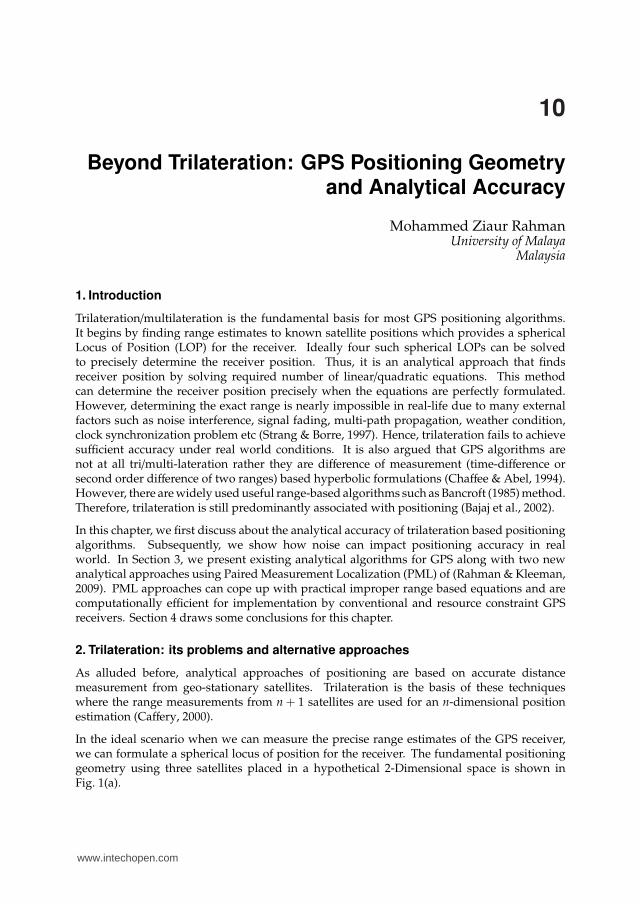
In the ideal scenario when we can measure the precise range estimates of the GPS receiver,we can formulate a spherical locus of position for the receiver. The fundamental positioninggeometry using three satellites placed in a hypothetical 2-Dimensional space is shown inFig. 1(a).

10

www.intechopen.com

2 Will-be-set-by-IN-TECH

(a) Ideal 2-D trilaterationscenario where linear formLOPs are found from thecorresponding two circularLOPs (Caffery, 2000).

L1

Same Linear LOP

r2r1

P1P2

ξ1

ξ2

(b) LOP from equidistant satellitesin presense of equal noise.

Fig. 1. Depiction of observation 1.

The circles surrounding the satellites with known positions p1 (x1, y1) , p2 (x2, y2) andp3 (x3, y3), denote the LOPs obtained from the individual range measurements for eachsatellite. Ideally, the LOPs surrounding satellite i is given by,

r2i = ‖pi − ρ‖

2 =((x− xi)

2 + (y− yi)2)

(1)

In 2-D, it is feasible to calculate the exact receiver position using only three rangemeasurements. Two range measurements can result in two solutions corresponding to theintersection of two circular LOPs. The third measurement resolves this ambiguity.

However, equating two circular LOPs will result in a straight line equation (in case of 3-D, itwill be planar equation) passing through two intersecting points of the circular LOPs. This linedoes not represent the actual locus of the receiver position as it will be clarified later. However,following (Caffery, 2000) this line is referred as Linear Form LOP in the subsequent discussions.In Fig. 1, L1 and L2 are determined from the circular LOPs corresponding to satellite pairs (p1,p2) and (p1, p3) respectively, with the intersection point (x, y) of L1 and L2 denoting the actualposition of the receiver.

As shown in Fig. 1,the positioning geometry works correctly for ideal case of exact rangeestimates being measured by the positioning devices. However, in reality it is quite difficult tomeasure the exact range both for external noise impact and internal errors such as receiver clockbias and satellite clock skews. However, we also showed the fact that accurate positioningcan be obtained if the noise effect is exactly the same for two satellites. However, in case ofvariable noise presence for two satellite range estimates usual linear form LOP obtained fromcircular LOPs deviates significantly from the true position of the receiver and leads to a badpositioning geometry. This is further explained as follows.

As it is clarified before that the range equations are mostly not accurate in practical scenario.Though trilateration is a mathematical approach and ideally it can find the exact receiverposition, however it cannot find the position very well when the range estimates are perturbedby noise. In this section we will specifically identify the problems of trilateration for inaccuraterange equations. For the ease of understanding we still limit this discussion for 2-dimensionsonly.

242 Global Navigation Satellite Systems – Signal, Theory and Applications

www.intechopen.com

Beyond Trilateration: GPS Positioning Geometry and Analytical Accuracy 3

0 5 10 15 20 25 30 35

5

10

15

20

25

30

35

X

YAnchor node

Regular node

Observed range

Actual range

Linear Form LOP

Hyperbolic LOP

(a)

5 10 15 20 25 30

5

10

15

20

25

30

35

X

Y

Anchor node

Regular node

Observed range

Actual range

Linear Form LOP

Hyperbolic LOP

(b)

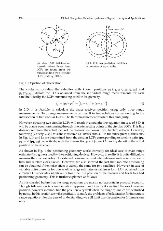
Fig. 2. The hyperbolic and linear form LOP of a receiver from range estimates by a pair ofsatellites under equal noise assumption. (a) The general case when two observed circularLOPs physically intersect. (b) The case when circular LOPs do not intersect due to noise andunderestimation of the ranges.

At first, we present the following observation that identifies the case when the conventionaltrilateration works in consideration of noise.

Observation 1. Assuming a receiver uses range estimates from two satellites that are located at thesame distance from the receiver and have equal noise components, it is shown below that the locus ofpositions for that receiver (as the error components vary) is a straight line whose equation is independentof range estimates.

Assume that due to noise, the range measurements for p1 (x1, y1), p2 (x2, y2) and p3 (x3, y3) arecorrupted to give respective LOPs of radii r1 = r1 + ξ1, r2 = r2 + ξ2 and r3 = r3 + ξ3, whereri, ri represent the observed and actual distance (pseudorange and actual range respectively)between the ith satellite and receiver respectively and ξi is the measurement noise at thereceiver corresponding to the measurement. The circular LOP can then be expressed as:

(ri + ξi)2 = ‖pi − ρ‖

2 (2)

where ρ = (x, y) is the receiver position to be determined.

Equating the circular LOPs for p1 and p2 using (2), L1 becomes:

(x2 − x1) x + (y2 − y1) y =

12

(‖p2‖

2 − ‖p1‖2 + (r1 + ξ1)

2− (r2 + ξ2)

2) (3)

where the right hand side becomes independent of range parameters, i.e., measurement valuesr1 and r2 whenever r1 = r2 ⇒ r1 + ξ1 = r2 + ξ2. One particular case is equidistant satellitesand equal noise presence when the above condition is fulfilled. �

The importance of this observation lies in the fact that it eliminates the signal propagationdependent parameters and receiver clock bias under assumed conditions completely.GPS measurements are mostly susceptible to these errors which are both device andenvironmentally dependent.

243Beyond Trilateration: GPS Positioning Geometry and Analytical Accuracy

www.intechopen.com


−20 0 20 40 60 80 100 120

−20

0

20

40

60

80

100

X

Y

Anchor node

Regular node

Observed range

Actual range

Linear Form LOP

Hyperbolic LOP

(a)

−20 0 20 40 60 80 100

−20

0

20

40

60

80

100

X

Y

Anchor node

Regular node

Observed range

Actual range

Linear Form LOP

Hyperbolic LOP

(b)

−50 0 50 100 150 200

−100

−50

0

50

100

150

X

Y

Anchor node

Regular node

Observed range

Actual range

Linear Form LOP

Hyperbolic LOP

(c)

−5 0 5 10 15 20 25 30

10

15

20

25

30

35

40

45

50

55

X

Y

Anchor node

Regular node

Observed range

Actual range

Linear Form LOP

Hyperbolic LOP

(d)

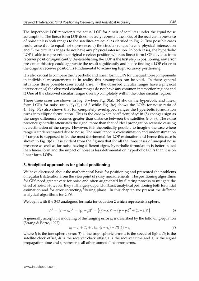
Fig. 3. The hyperbolic and linear form LOPs for unequal noise presence. (a) The general casewhen two observed circular LOPs physically intersect. (b) The case when observed circularLOPs do not intersect due to underestimation of the ranges. (c) The case when observedcircular LOPs do not intersect but overlap completely due to overestimation of the ranges.(d)The case when ranging errors are of opposite signs.

Assuming equal noise presence, it is useful to explore paired measurements rather thanindividual ranges to mitigate the effect of noise. As the difference of the range estimatesequate to actual difference for equal noise presence (e.g., r2 − r1 = r2 − r1), the LOP for thereceiver position is found by the locus of positions maintaining constant difference from thepair of satellites. Hence, the hyperbolic LOP of the receiver can be found independent of thenoise parameters as shown in Fig. 2 and formulated below:

√(x− x2)

2 + (y− y2)2−

√(x− x1)

2 + (y− y1)2 = (r2 − r1) (4)

After algebraic manipulations, it takes the general hyperbolic form as follows for p1 =(0, 0), p2 = (a, 0), and r1 − r2 = c.

(x−

a

2

)2−

y2

(a2

c2 − 1) = c2

4(5)


www.intechopen.com


The hyperbolic LOP represents the actual LOP for a pair of satellites under the equal noiseassumption. The linear form LOP does not truly represent the locus of the receiver in presenceof noise unless both ranges to the satellites are equal as clarified in Fig. 2. Two possible casescould arise due to equal noise presence: a) the circular ranges have a physical intersectionand b) the circular ranges do not have any physical intersection. In both cases, the hyperbolicLOP is able to represent the original receiver position whereas linear form LOP deviates fromreceiver position significantly. As establishing the LOP is the first step in positioning, any errorpresent at this step could aggravate the result significantly and hence finding a LOP closer tothe original receiver position is fundamental to achieving high accuracy positioning.

It is also crucial to compare the hyperbolic and linear form LOPs for unequal noise componentsin individual measurements as in reality this assumption can be void. In these generalsituations three possible cases could arise. a) the observed circular ranges have a physicalintersection; b) the observed circular ranges do not have any common intersection region; andc) One of the observed circular ranges overlap completely within the other circular region.

These three cases are shown in Fig. 3 where Fig. 3(a), (b) shows the hyperbolic and linearform LOPs for noise ratio (ξ1/ξ2) of 2 while Fig. 3(c) shows the LOPs for noise ratio of4. Fig. 3(c) also shows that for completely overlapped ranges the hyperbolic formulationturns into elliptic formulation. This is the case when coefficient of y2 in (5) changes sign asthe range difference becomes greater than distance between the satellites (c > a). The noisepresence generally attenuates the signal more than that of ideal propagation scenario causingoverestimation of the range. However, it is theoretically possible to imagine the case whererange is underestimated due to noise. The simultaneous overestimation and underestimationof ranges is supposed to be the most detrimental for LOP estimation and hence this case isshown in Fig. 3(d). It is evident from the figures that for all the three cases of unequal noisepresence as well as for noise having different signs, hyperbolic formulation is better suitedthan linear form and the impact of noise is less detrimental on hyperbolic LOPs than it is onlinear form LOPs.

3. Analytical approaches for global positioning

We have discussed about the mathematical basis for positioning and presented the problemsof regular trilateration from the viewpoint of noisy measurements. The positioning algorithmsfor GPS need greater care for noise and often augmented by filtering process to mitigate theeffect of noise. However, they still largely depend on basic analytical positioning both for initialestimation and for error correcting/filtering phase. In this chapter, we present the differentanalytical algorithms for GPS.

We begin with the 3-D analogous formula for equation 2 which represents a sphere.

ri2 = (ri + ξi)

2 = ‖pi − ρ‖2 =((x− xi)

2 + (y− yi)2 + (z− zi)

2)

(6)

A generally acceptable modeling of the ranging error ξi is described by the following equation(Strang & Borre, 1997).

ξi = Ii + Ti + c (dti(t− τi) − dt(t)) − ei (7)

where Ii is the ionospheric error, Ti is the tropospheric error, c is the speed of light, dti is thesatellite clock offset, dt is the receiver clock offset, t is the receiver time and τi is the signalpropagation time and ei represents all other unmodelled error terms.


www.intechopen.com


The equation 6 can be iteratively solved using Newton’s method. However, the iterativeapproach will be computationally expensive. Moreover, the positioning accuracy will be pooras there is no proper formalism to identify and mitigate the error components.

3.1 Ordinary trilateration for positioning

Let Pi =(pi

1, pi

2

)be an arbitrary satellite pair, where pi

1=(xi

1, yi

1, zi

1

)and pi

2=(xi

2, yi

2, zi

2

)

represent satellite positions of the ith pair. Analogous to 2-D linear form LOP of equation 3, a3-D planar form LOP is found as follows.

(xi

2 − xi1

)x +(yi

2 − yi1

)y +(zi

2 − zi1

)z =

12

(‖pi

2‖2 − ‖pi

1‖2 +(ri1

)2−(ri

2

)2+ 2ξ

(ri

1 − ri2

)) (8)

Where it is assumed that the noise are equal and constant for a particular satellite pair i.e.,ξ1 = ξ2 = ξ.

The equation becomes linear in terms of x, y, z and ξ if the noise is represented by a singleparameter ξ for all pairs. In that case there are four unknowns in this equation and thereforefour equations will be required to solve them. In practicality, the assumption is susceptiblefor large positioning error and hence iterative refinement approach of the following is ratheradopted for real implementations.

3.2 Iterative least squares estimate

The iterative approach works by having a preliminary estimate of the receiver position (ρ0 =[x0y0z0]T). Let the rotation rate of the earth be ω. The position vectors in the earth centeredearth fixed (ECEF) system of the receiver be donated by ρ(t)ECEF and geo-stationary positionvector for satellite i be denoted by pi(t)geo where the argument t denotes the dependence ontime. The range equation can be written as:

ri = ‖R3(ωτi)pi(t− τi)geo − ρ(t)ECEF‖ (9)

Where R3 is the earth’s rotation matrix as defined below.

R3(ωτi) =

⎡⎢⎢⎢⎢⎢⎢⎣

cos(ωτi) sin(ωτi) 0− sin(ωτi) cos(ωτi) 0

0 0 1

⎤⎥⎥⎥⎥⎥⎥⎦

Let ⎡⎢⎢⎢⎢⎢⎢⎣xi

yi

zi

⎤⎥⎥⎥⎥⎥⎥⎦ = R3(ωτi)pi(t− τi)geo and

⎡⎢⎢⎢⎢⎢⎢⎣xyz

⎤⎥⎥⎥⎥⎥⎥⎦ = ρ(t)ECEF (10)

Now, omitting the refraction terms Ii and Ti and linearizing the equation 6, we get

−xi − x0

(ri)0δx−

yi − y0

(ri)0δy−

zk − z0

(ri)0δz + (c dt) = ri − (ri)

0 − ǫi = bi − ǫi (11)

where bi denotes the correction to the preliminary range estimate.


www.intechopen.com


When more than four observations are available we can compute the correction values⟨δ x, δ y, δ z

⟩for the preliminary estimate. The least squares formulation can be concisely

written as follows.

Ax =

⎡⎢⎢⎢⎢⎢⎢⎢⎢⎢⎢⎢⎢⎢⎢⎢⎢⎢⎢⎣

−x1−x0

r1−

y1−y0

r1−

z1−z0

r11

−x2−x0

r2−

y2−y0

r2−

z2−z0

r21

......

......

−xm−x0

rm−

ym−y0

rm−

zm−z0

rm1

⎤⎥⎥⎥⎥⎥⎥⎥⎥⎥⎥⎥⎥⎥⎥⎥⎥⎥⎥⎦

⎡⎢⎢⎢⎢⎢⎢⎢⎢⎢⎢⎣

δxδyδzδc dt

⎤⎥⎥⎥⎥⎥⎥⎥⎥⎥⎥⎦= b− ǫ (12)

The least squares solution is

⎡⎢⎢⎢⎢⎢⎢⎢⎢⎢⎢⎣

δxδyδzδc dt

⎤⎥⎥⎥⎥⎥⎥⎥⎥⎥⎥⎦= (AT

Σ−1A)−1AT

Σ−1b (13)

If the code observations are independent and assumed to have equal variance, then the abovecan be simplified to ⎡

⎢⎢⎢⎢⎢⎢⎢⎢⎢⎢⎣

δxδyδzδc dt

⎤⎥⎥⎥⎥⎥⎥⎥⎥⎥⎥⎦= (ATA)−1ATb (14)

The final position vector can be estimated by ρ =[x0 + δx y0 + δy z0 + δz

]T.

3.3 Bancroft’s method (least squares solution)

We want to turn positioning into a linear algebra problem. Here is a clever method due toBancroft (1985) that does some algbraic manipulations to reduce the equations to a least-squaresproblem. Multiplying things out in equation 6 and using the receiver clock bias −b = ξ′

is as

the only noise parameter, we get

x2i − 2xix + x2 + y2

i − 2yiy + y2 + z2i − 2ziz + z2 = r2

i − 2rib + b2 (15)

Rearranging,

(x2

i + y2i + z2

i − r2i

)− 2 (xix + yiy + ziz− rib) +

(x2 + y2 + z2 − r2

)= 0 (16)

Let ρ = [x y z r]T denote the receiver position vector and pi = [xi yi zi ri]T denote the ith satellite

position and range vectors.

Using Lorentz inner product for 4-space defined by:

〈�u, �v〉 = u1v1 + u2v2 + u3v3 − u4v4

Equation 16 can be rewritten as:

1

2〈pi, pi〉 − 〈pi,ρ〉+

1

2〈ρ,ρ〉 = 0; (17)


www.intechopen.com


In order to apply least squares estimation the equations for each satellite are organized asfollows:

B =

⎡⎢⎢⎢⎢⎢⎢⎢⎢⎢⎢⎢⎢⎢⎢⎢⎢⎢⎢⎣

x1 y1 z1 −r1

x2 y2 z2 −r2

......

......

xm ym zm −rm

⎤⎥⎥⎥⎥⎥⎥⎥⎥⎥⎥⎥⎥⎥⎥⎥⎥⎥⎥⎦

,

a =1

2

⎡⎢⎢⎢⎢⎢⎢⎢⎢⎢⎢⎢⎢⎢⎢⎢⎢⎢⎢⎣

〈p1, p1〉

〈p2, p2〉

...

〈pm, pm〉

⎤⎥⎥⎥⎥⎥⎥⎥⎥⎥⎥⎥⎥⎥⎥⎥⎥⎥⎥⎦

, e =

⎡⎢⎢⎢⎢⎢⎢⎢⎢⎢⎢⎢⎢⎢⎣

11...1

⎤⎥⎥⎥⎥⎥⎥⎥⎥⎥⎥⎥⎥⎥⎦

, and ∧ =1

2〈ρ,ρ〉

We can now rewrite equation 17 as:

a−Bρ+ ∧e = 0

⇒ Bρ = a + ∧e (18)

For more than 4 satellites, we can have closed form least squares solution as follows:

ρ = B+a + ∧e (19)

where B+ = (BTB)−1BT is the pseudoinverse of Matrix B.

However, the solution ρ involves ∧ which is defined in terms of unknown ρ. This problemis avoided by substituting ρ into the definition of the scalar ∧ and using the linearity of theLorentz inner product as follows:

∧ =1

2

⟨B+ (a + ∧e) , B+ (a + ∧e)

⟩

After rearranging,

∧2〈B+e, B+e〉+ 2∧(〈B+�e, B+a〉 − 1

)+ 〈B+a, B+a〉 = 0 (20)

This is a quadratic equation in ∧ with coefficients 〈B+e, B+e〉, 2 (〈B+e, B+a〉 − 1), and〈B+a, B+a〉. All these three values can be computed and we can solve for two possible valuesof ∧ using the quadratic equation. If we get the two solutions to this equation ∧1 and ∧2, thenwe can solve for two possible solutions ρ1 and ρ2 in equation 19. One of these solutions willmake sense, it will be on the surface of the earth (which has a radius of approximately 6371km), and one will not.

The major advantage of the Bancroft’s method is to have a closed form least squares solution forGPS equations. It has the same advantage of least squares approach of using all the availablesatellites for location estimation. On the contrary, it uses the fundamental equation of sphericalranging that in the course of solution leads to planar form LOPs which are than hyperboloidLOPs. Therefore as discussed before, this method cannot be used for high-accuracy positioningin presence of noise.


www.intechopen.com


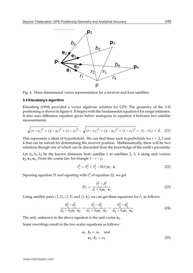
Fig. 4. Three dimensional vector representation for a receiver and four satellites.

3.4 Kleusberg’s algorithm

Kleusberg (1994) provided a vector algebraic solution for GPS. The geometry of the 3-Dpositioning is shown in figure 4. It begins with the fundamental equation 6 for range estimates.It also uses difference equation given below analogous to equation 4 between two satellitemeasurements.

√(x− xi)

2 + (y− yi)2 + (z− zi)

2−

√(x− x1)

2 + (y− y1)2 + (z− z1)

2 = (ri − r1) = di (21)

This represents a sheet of hyperboloid. We can find three such hyperboloids for i = 2, 3 and4 that can be solved for determining the receiver position. Mathematically, there will be twosolutions though one of which can be discarded from the knowledge of the earth’s proximity.

Let b2, b3, b4 be the known distances from satellite 1 to satellites 2, 3, 4 along unit vectorse2, e3, e4. From the cosine law for triangle 1− i− ρ,

r2i = b2

i + r21 − 2bir1e1 · ei (22)

Squaring equation 21 and equating with r2i

of equation 22, we get

2r1 =b2

i− d2

i

di + bie1 · ei(23)

Using satellite pairs (1, 2), (1, 3) and (1, 4); we can get three equations for r1 as follows:

b22− d2

2

d2 + b2e1 · e2=

b23− d2

3

d3 + b3e1 · e3=

b24− d2

4

d4 + b4e1 · e4(24)

The only unknown in the above equation is the unit vector e1.

Some rewritings result in the two scalar equations as follows:

e1 · f2 = u2 and

e1 · f3 = u3 (25)


www.intechopen.com


Where for m = 2, 3;

Fm = bm

b2m−d2

mem −

bm+1

b2m+1−d2

m+1

em+1

fm = Fm

‖Fm‖

um = 1‖Fm‖

(dm+1

b2m+1−d2

m+1

−dm

b2m−d2

m

)

The unit vector f2 lies in the plane through satellites 1, 2 and 3. This plane is spanned by e2

and e3. Similarly f3 is in the plane determined by satellites 1, 3 and 4.

Equation 25 determines the cosine of the two unit vectors f2 and f3 with the desired unit vectore1. It will have two solutions, one above and one below the plane spanned by f2 and f3. In casethese vectors are parallel their inner product is zero and there are infinitely many solutionsand hence the position cannot be determined.

The algebraic solution to equation 25 can be derived using vector triple product identity,

e1 × (f1 × f2) = f1 (e1 · f2) − f2 (e1 · f1)

All the terms in the right hand of the above equation is readily computed using u2, u3.Substituting h for the right hand side and g for f1 × f2, we get

e1 × g = h (26)

Multiplying both sides of the equation by g and applying the vector triple product identity,

e1 (g · g) − g (g · e1) = g× h (27)

The scalar product in the second term of the left-hand side can be written in terms of the angleθ between unit vector e1 and g as follows

g · e1 = [g · g]12 cosθ

The sine value of the angle can be found from equation 26 as follows:

[h · h]12 = [(e1 × g) · (e1 × g)]

12 = [g · g]

12 sinθ

Using the sine value in the cosine formula above, we obtain,

g · e1 = ± [g · g]12

[1−

h · h

g · g

] 12

= ± [g · g− h · h]12

Substituting the above into equation 27, we obtain the desired solution:

e1 =1

2

(g× h± g

√g · g− h · h

)(28)

The two values can be put in equation 24 to check the correctness of the value. The correctparameter will result in a intersection point that lies on the earth’s surface and hence must have


www.intechopen.com


a distance of about 6371 km from the origin. We can eventually get the receiver coordinateusing correct value of e1 as follows:

ρ = p1 + r1e1 (29)

The Kleusberg’s method is geometrically oriented and uses a minimum number of satellites.On the other hand, it cannot utilize more number of satellites even when they are available. Thismethod is also dependent on the proper geometrical orientation of the satellites. Moreover,it often gives different results for different set of satellites and depending on the order of thesatellites in solving the equations.

3.5 Paired measurement localization

In trilateration, the positioning works by simultaneous solution of three spherical LOPequations. Similar to the 2-D steps, we can equate two spherical LOP equations to findequation for a 2-D plane representing the planar locus of position. Analogous to 2-D case,three planar equations can be solved to find the ultimate receiver position.

As shown in section 2, the effect of noise will have detrimental impact on the aforementionedsimple solution. On the other hand, instead of equating the two imprecise range equations wecan maintain an equi-distant locus of position from two satellites as formulated in equation 21for a hyperboloid LOP. This will be more accurate than a traditional 2-D planar LOP basedpositioning.

Solving the nonlinear hyperbolic/hyperboloid equations is difficult. Moreover, existinghyperbolic positioning methods proceed by linearizing the system of equations using eitherTaylor-series approximation (Foy, 1976; Torrieri, 1984) or by linearizing with another additionalvariable (Chan & Ho, 1994; Friedlander, 1987; Smith & Abel, 1987). However, while linearizingworks well for existing approaches it is not readily adaptable for the proposed paired approachas linearizing is indeed pairing with an arbitrarily chosen hyperbolic LOP. The assumptionof equal noise cannot be held for any arbitrary selection of pairs and hence alternate ways tosolve such LOPs for paired measurement is now formulated.

3.6 PML with single reference satellite

(Chan & Ho, 1994) provided closed form least squares solution for non-linear hyperbolic LOPsby linearizing with reference to a single satellite. Analogous to their approach a closed formsolution is found for PML using pairs having a common reference satellite in them. Thesolution is simpler than (Chan & Ho, 1994)’s approach as the effect of noise is considered earlyin the paired measurements formulations.

Let ri j

represent the difference in the observed ranges for satellite pairs (i, j). In case of equal

noise presence it follows:

ri j= r

i j= ri − r j

After squaring and rearranging,

r2i = r2

i j+ 2r

i jr j + r2

j

(30)

Hence, the actual spherical LOP can be transformed as follows:

(x− xi)2 + (y− yi)

2 + (z− zi)2 = (r

i j)2 + 2r

i jr j + (r j)

2 (31)


www.intechopen.com


Using (31) for pairs (pi, p j) = (pk, p1) and (pl, p1) and subtracting the second from the first,

− (xk − xl)x− (yk − yl)y− (zk − zl)y− (rk1− r

l1)r1 = 1

2

((r

k1)2 − (r

l1)2 − ‖pk‖

2 + ‖pl‖2)

(32)

where ‖pk‖2 = (x2

k+ y2

k). The above formulation represents a set of linear equations with

unknowns x, y, z and r1 for all combination of two pair of satellites having satellite 1 in common.Let x

i j, y

i j, z

i jrepresent the difference xi − x j, yi − y j, zi − z j respectively, Ci represent the ith

combination and m represent the total number of combinations with Ci = {(pki, p1), (pli , p1)}.

The system of linear equations for these m combinations can be concisely written as follows:

AX = B (33)

where,

A = −

⎡⎢⎢⎢⎢⎢⎢⎢⎢⎢⎢⎢⎢⎢⎢⎢⎢⎢⎢⎢⎣

xk1l1

yk1l1

zk1l1−

(r

k11− r

l11

)

xk2l2

yk2l2

zk2l2−

(r

k21− r

l21

)

. . .

xkmlm

ykmlm

zkmlm−

(r

km1− r

lm1

)

⎤⎥⎥⎥⎥⎥⎥⎥⎥⎥⎥⎥⎥⎥⎥⎥⎥⎥⎥⎥⎦

,

X =

⎡⎢⎢⎢⎢⎢⎢⎢⎢⎢⎢⎣

xyzr1

⎤⎥⎥⎥⎥⎥⎥⎥⎥⎥⎥⎦

, B =1

2

⎡⎢⎢⎢⎢⎢⎢⎢⎢⎢⎢⎢⎢⎢⎣

(rk11

)2 − (rl11)2 − ‖pk1

‖2 + ‖pl1‖2

(rk21

)2 − (rl21)2 − ‖pk2

‖2 + ‖pl2‖2

.(r

km1)2 − (r

lm1)2 − ‖pkm

‖2 + ‖plm‖2

⎤⎥⎥⎥⎥⎥⎥⎥⎥⎥⎥⎥⎥⎥⎦

For m ≥ 3, the system of equations can be solved. However, r1 is related to x, y, z by (6). Forpairing and equivalence of ri − r1 = ri − r1, observed ranges are always used in the equationsand thus the system of equations are essentially independent of relationship between (x, y, z)and r1. This is also verified by the iterative refinement of r1 where r1 is modified by obtained r1

in successive runs. The results show no difference in position estimates (x, y, z) for successiveiterations.

The equal noise assumption cannot be applied to any arbitrary selection of pairs while it isquite reasonable for satellites observing near equal ranges to have equal noise components.The selection of pairs with near equal ranges from a single reference satellite, may not befeasible for low visibility where only a very few satellites are available for positioning. This isthe motivation for the next solution approach.

3.7 PML with refinement of the locus of positions

The linearization using one single reference satellite raises a performance issue and while itis superior to trilateration in most of the cases, occassionally it performs worse. In search fora positioning approach that can give consistently better estimates than basic trilateration, alocus refinement approach is now presented.

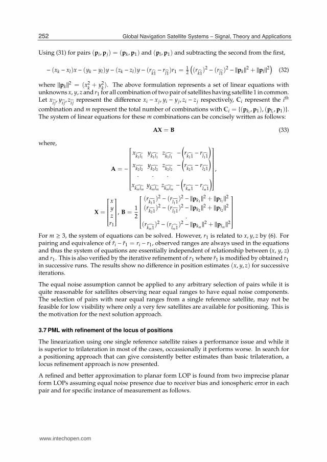
A refined and better approximation to planar form LOP is found from two imprecise planarform LOPs assuming equal noise presence due to receiver bias and ionospheric error in eachpair and for specific instance of measurement as follows.


www.intechopen.com


Li

L i

Lj

L j

Lk

L k

Oi

Oj

Ok

I ijk

Iijk

I

Ii j k

Iij k

Ii jk

Ii jk

Iij k

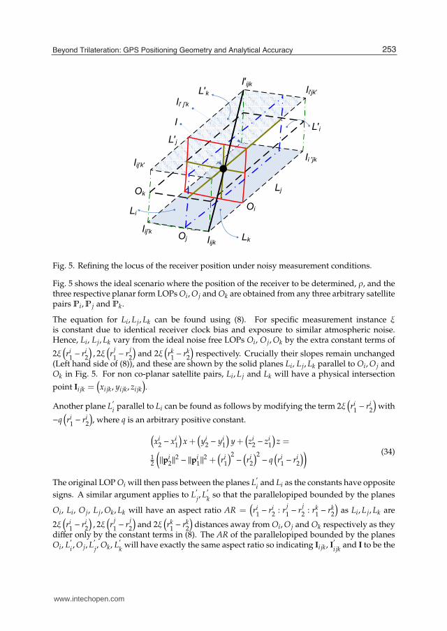
Fig. 5. Refining the locus of the receiver position under noisy measurement conditions.

Fig. 5 shows the ideal scenario where the position of the receiver to be determined, ρ, and thethree respective planar form LOPs Oi, O j and Ok are obtained from any three arbitrary satellitepairs Pi, P j and Pk.

The equation for Li, L j, Lk can be found using (8). For specific measurement instance ξis constant due to identical receiver clock bias and exposure to similar atmospheric noise.Hence, Li, L j, Lk vary from the ideal noise free LOPs Oi, O j, Ok by the extra constant terms of

2ξ(ri1− ri

2

), 2ξ(r

j

1− r

j

2

)and 2ξ

(rk1− rk

2

)respectively. Crucially their slopes remain unchanged

(Left hand side of (8)), and these are shown by the solid planes Li, L j, Lk parallel to Oi, O j andOk in Fig. 5. For non co-planar satellite pairs, Li, L j and Lk will have a physical intersection

point Ii jk =(xi jk, yi jk, zi jk

).

Another plane L′

iparallel to Li can be found as follows by modifying the term 2ξ

(ri1− ri

2

)with

−q(ri1− ri

2

), where q is an arbitrary positive constant.

(xi

2 − xi1

)x +(yi

2 − yi1

)y +(zi

2 − zi1

)z =

12

(‖pi

2‖2 − ‖pi

1‖2 +(ri

1

)2−(ri

2

)2− q(ri

1 − ri2

)) (34)

The original LOP Oi will then pass between the planes L′

iand Li as the constants have opposite

signs. A similar argument applies to L′

j, L′

kso that the parallelopiped bounded by the planes

Oi, Li, O j, L j, Ok, Lk will have an aspect ratio AR =(ri

1− ri

2: r

j

1− r

j

2: rk

1− rk

2

)as Li, L j, Lk are

2ξ(ri

1− ri

2

), 2ξ(r

j

1− r

j

2

)and 2ξ

(rk

1− rk

2

)distances away from Oi, O j and Ok respectively as they

differ only by the constant terms in (8). The AR of the parallelopiped bounded by the planesOi, L

′

i, O j, L

′

j, Ok, L

′

kwill have exactly the same aspect ratio so indicating Ii jk, I

′

i jkand I to be the


www.intechopen.com


diagonal points of the parallelopiped where I′

i jkdenotes the intersection point of planes L

′

i, L′

j

and L′

k.

Hence, the equation of the actual LOP Ii jkI′

i jkpassing through I is found from the three

intersection points Ii jk, Ii j′ k and Ii′ j′ k′ which are available from equations (8) and (34) and

analogous equations for LOPs L j, Lk, L′

jand L

′

k.

As the LOPs obtained in this way are expressed by linear equations with unknowns x, y andz, they can be solved using simple algebraic or least squares methods.

The locus refinement formulation assumes noise to be present in the formulae. However, if thenoise is absent the diagonal points Ii jk and I

′

i jkwould be very close and during the calculation

process whenever pairs having distance < 2m are observed the estimated location is found asthe mean of these two points.

The planar form LOP obtained from each satellite pair must be linearly independent so theydo not represent either the same or a parallel planar LOP. Such satellite pairs are referred to asmutually independent, so a key objective is to identify such satellite pairs where each satellitehas nearly similar distance from the receiver. PML may be intuitively viewed as positioningexploiting bearing measurements, as LOPs effectively denote a directional line. It is known thatangular measurements are consistently more accurate compared to TOF range measurementsand in (Chintalapudi et al., 2004) a combination of range and angular measurement has beenshown to achieve better positioning results, providing a valuable insight as to why the LOPrefinement furnishes better location estimation.

3.8 Selection of satellite pairs for PML

It is apparent from observation 1 that the existence of a pair of satellites having equal distancefrom the receiver position can have equal atmospheric noise exposure, with this prerequisitebeing relaxed and generalized by LOP refinement approach. Observation 1 highlights thesignificance of pairing the satellites for better noise cancellation and a better selection processcan result in considerable improvement. With practical range estimations there is no explicitway to determine the best possible pairs following the observation. However, the rangeestimation ratios can be used as a rough measure for adhering to observation 1 which is thebasis for the following empirically defined ranking criteria. The ranking criteria also considersthe closeness of the satellites. If the two satellites are too close to each other they might havethe best range estimation ratio while effectively they are like two satellites placed at the sameplace and hence providing no additional redundancy to help positioning. Utilizing, the abovementioned two principles the following empirical ranking criteria is introduced.

=r1

r2

(1

‖p1p2‖

)(35)

where r1 and r2 are the observed range estimates for satellite pair (p1, p2) such that r1 ≥ r2 and‖p1p2‖ is the Euclidean distance between the two satellites. The pairs having lower ranks ()are preferred over ones with higher ranks. The complete satellite selection algorithm is givenas follows.

Algorithm 1 searches all available satellites for a particular receiver so its computationalcomplexity is O(available satellites2) if an exhaustive search is applied. This selection process


www.intechopen.com


Algorithm 1 Satellite Selection for PML Refinement Approach

for all pair of neighboring satellites do

Calculate rank () for the pair(pi, p j

);

if(pi, p j

)is co-planar with any previous selected pair and () of present pair is lower

than selected pair thenReplace the previous co-planar pair with current pair

elseif Number of selected pair < Required number of pairs then

Add the current pair to the selected pairselse

Replace the worst ranking selected pair with the current pairend if

end ifend for

can be run on-demand only when satellite positions are either changed or after considerablemovement of the receiver. Given the small number of visible satellites in range, this will incurnegligible cost.

Finally, as the new PML method itself is an analytical approach, the order of computationalcomplexity is O(1) once satellite selection has been completed.

Summarizing, PML approaches are improvement over basic trilateration in that it considersnoisy measurement conditions in its formulation. Thus, this new strategy performssignificantly better for real time GPS and tracking performance.

4. Conclusion

This chapter presented a detailed discussion on the analytical approaches for GPS positioning.Trilateration is the basis for most analytical positioning approaches and hence this chapterbegins with fundamental discussion on trilateration. However, it performs poorly undernoisy conditions which is analyzed in detail from theoretical and simulated scenarios. Wealso showed how difference of two range measurements can result in better positioningformulations. Subsequently, we present existing analytical approaches of Bancroft’s methodand Kleusberg’s method that uses least squares and vector algebra respectively for solution ofGPS equations. Later we present two newer approaches that are based on using better LocusOf Position (LOP) for the receiver than customary spherical locus in presence of noise. Thefirst of these, called Paired Measurement Localization (PML) with single reference satelliteuses hyperboloid planar locus of positions. The solution of these non-linear hyperboloids arefound by linearizing with reference to a single satellite. The other PML approach obtains abetter LOP from ordinary planar LOPs using a LOP refinement technique. Both of the PMLbased approaches have the advantage that they can utilize all the available satellites usingleast squares solution. If only four/three LOPs are used for PML single reference or PMLLOP refinement respectively, the receiver position can be calculated by simple algebra. Thishas the advantage of avoiding matrix inversion for least squares solution and particularlysuitable when the receiver has constraint computational support such as mobile embeddedGPS receivers. Alternatively, when sufficient computational resources are available and better


www.intechopen.com


precision is needed full fledged least squares solution and further filtering techniques couldbe applied.

Part of this research is supported by University of Malaya high-impact research grant numberUM.C/HIR/MOHE/FCSIT/04.

Bajaj, R., Ranaweera, S. & Agrawal, D. (2002). GPS: Location-tracking technology, Computer35(4): 92–94.

Bancroft, S. (1985). An algebraic solution of the GPS equations, IEEE Transactions on Aerospaceand Electronic Systems 21(6): 56–59.

Caffery, J. J. (2000). A new approach to the geometry of TOA location, 52nd Vehicular TechnologyConference.

Chaffee, J. & Abel, J. (1994). On the exact solutions of pseudorange equations, IEEE Transactionson Aerospace and Electronic Systems 30: 1021–1030.

Chan, Y. & Ho, K. (1994). A simple and effificient estimator for hyperbolic location, IEEETransactions on Signal Processing 42: 1905–1915.

Chintalapudi, K. K., Dhariwal, A., Govindan, R. & Sukhatme, G. (2004). Ad-hoc localizationusing ranging and sectoring, INFOCOM.

Foy, W. H. (1976). Position-location solutions by Taylor-series estimation, IEEE Trans. Aerosp.Electron. Syst. 12: 187–194.

Friedlander, B. (1987). A passive localization algorithm and its accuracy analysis, IEEE J. Ocean.Eng. 12: 234–245.

Kleusberg, A. (1994). Analytical GPS navigation solution, pp. 1905–1915.Rahman, M. Z. & Kleeman, L. (2009). Paired measurement localization: A robust approach for

wireless localization, IEEE Transactions on Mobile Computing 8(8).Smith, J. O. & Abel, J. S. (1987). Closed-form least-squares source location estimation

from range-difference measurements, IEEE Trans. Acoust., Speech, Signal Process.35: 1661–1669.

Strang, G. & Borre, K. (1997). Linear Algebra, Geodesy, and GPS, Wellesley-Cambridge.Torrieri, D. J. (1984). Statistical theory of passive location systems, IEEE Trans. Aerosp. Electron.

Syst. 20: 183–197.

5. Acknowledgment

6. References


www.intechopen.com

Global Navigation Satellite Systems: Signal, Theory andApplicationsEdited by Prof. Shuanggen Jin

ISBN 978-953-307-843-4Hard cover, 426 pagesPublisher InTechPublished online 03, February, 2012Published in print edition February, 2012

InTech EuropeUniversity Campus STeP Ri Slavka Krautzeka 83/A 51000 Rijeka, Croatia Phone: +385 (51) 770 447 Fax: +385 (51) 686 166www.intechopen.com

InTech ChinaUnit 405, Office Block, Hotel Equatorial Shanghai No.65, Yan An Road (West), Shanghai, 200040, China

Phone: +86-21-62489820 Fax: +86-21-62489821

Global Navigation Satellite System (GNSS) plays a key role in high precision navigation, positioning, timing,and scientific questions related to precise positioning. This is a highly precise, continuous, all-weather, andreal-time technique. The book is devoted to presenting recent results and developments in GNSS theory,system, signal, receiver, method, and errors sources, such as multipath effects and atmospheric delays.Furthermore, varied GNSS applications are demonstrated and evaluated in hybrid positioning, multi-sensorintegration, height system, Network Real Time Kinematic (NRTK), wheeled robots, and status and engineeringsurveying. This book provides a good reference for GNSS designers, engineers, and scientists, as well as theuser market.

How to referenceIn order to correctly reference this scholarly work, feel free to copy and paste the following:

Mohammed Ziaur Rahman (2012). Beyond Trilateration: GPS Positioning Geometry and Analytical Accuracy,Global Navigation Satellite Systems: Signal, Theory and Applications, Prof. Shuanggen Jin (Ed.), ISBN: 978-953-307-843-4, InTech, Available from: http://www.intechopen.com/books/global-navigation-satellite-systems-signal-theory-and-applications/beyond-trilateration-gps-positioning-geometry-and-analytical-accuracy

© 2012 The Author(s). Licensee IntechOpen. This is an open access articledistributed under the terms of the Creative Commons Attribution 3.0License, which permits unrestricted use, distribution, and reproduction inany medium, provided the original work is properly cited.

http://creativecommons.org/licenses/by/3.0

Date post:	13-Mar-2022
Category:	Documents
Upload:	others
View:	6 times
Download:	0 times

Beyond Trilateration: GPS Positioning Geometry and Analytical

Documents