23
Bezier Curves and Splines David Eno MAT 499 Fall ‘06
| Date post: | 18-Dec-2015 |
| Category: |
Documents |
| Upload: | lambert-elliott |
| View: | 220 times |
| Download: | 2 times |
Bezier Curves and Splines
David Eno
MAT 499
Fall ‘06

Introduction
• In Engineering, one often wants a smooth curve through a set of known points.
• In Physics, a smooth curve is required to represent the shape of a deflected beam.
• Computer Aided Design and Manufacturing programs like lines and circular arcs.– Lots of things cannot be conveniently
described by lines and circular arcs.

Bézier Curves
• Bézier Curves were first developed in 1959 by Paul de Casteljau.
• They were popularized in 1962 by French engineer Pierre Bézier, who used them to design automobile bodies.

Quadratic Bézier Curves
• Given three points P0, P1, and P2, a quadratic Bézier curve is the path traced by the parabolic function:
10 where
)1(2)1()( 221
20
t
tPttPtPtx

Quadratic Bézier Curve
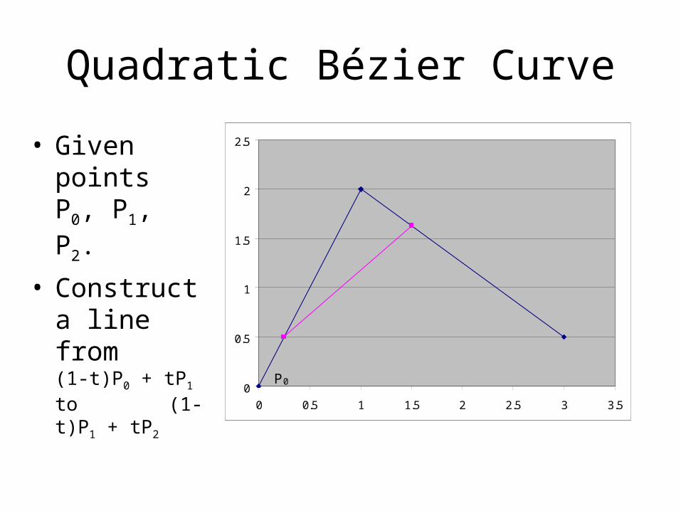
• Given points P0, P1, P2.
0
0.5
1
1.5
2
2.5
0 0.5 1 1.5 2 2.5 3 3.5
P0
P1
P2
Quadratic Bézier Curve
• Given points P0, P1, P2.
• Construct a line from (1-t)P0 + tP1 to (1-t)P1 + tP2
0
0.5
1
1.5
2
2.5
0 0.5 1 1.5 2 2.5 3 3.5
P0
P1
P2
(1-t)P0 + tP1
(1-t)P1 + tP2

Quadratic Bézier Curve
• Given points P0, P1, P2.
• Construct a line from (1-t)P0 + tP1 to (1-t)P1 + tP2
• The point, x, is on the curve.
0
0.5
1
1.5
2
2.5
0 0.5 1 1.5 2 2.5 3 3.5
P0
P1
P2
(1-t)P0 + tP1
(1-t)P1 + tP2
(1-t)2P0 + 2t(1-t)P1 + t2P2

Quadratic Bézier Curve
• Given points P0, P1, P2.
• Construct a line from (1-t)P0 + tP1 to (1-t)P1 + tP2
• The point, x, is on the curve.
0
0.5
1
1.5
2
2.5
0 0.5 1 1.5 2 2.5 3 3.5
P0
P1
P2
(1-t)P0 + tP1
(1-t)P1 + tP2
(1-t)2P0 + 2t(1-t)P1 + t2P2

Bézier Curve Advantages
• 3 points uniquely determine a parabola.
• It’s easy to calculate points.
• The numerical algorithm is stable. (i.e. given reasonable input, the algorithm won’t blow up.)

Cubic Bézier Curve• Extending this method to use four points, we can
construct a cubic curve.
0
0.2
0.4
0.6
0.8
1
1.2
0 0.5 1 1.5 2 2.5 3 3.5
P0
P1
P2
P3
(1-t)3P0 + 3t(1-t)2P1 + 3t2(1-t)P2 + t3P3

In General…
• To construct an nth degree Bezier curve, you need n+1 control points.
• The formula for a point on the curve is:
iini
n
i
Ptti
ntx
)1()(
0

Recursion
• Pseudo code for recursive technique:makeBezier(Control Points)
If points are collinear enoughOutput last point
ElseSubdivide points
makeBezier(Left Control Points)
makeBezier(Right Control Points)
End If

Bezier Splines
• We typically want a smooth curve that passes though a set of points.
• Problem: The first and last control points are the only ones guaranteed to be on a Bezier Curve.
• A Solution: Use Bezier Splines, which are composite (i.e. piecewise) Bezier Curves.– But then we need to compute control points.

Cubic Bezier Splines
• We could make splines from Bezier curves of any degree.
• We choose cubic (degree = 3) curves for the following reasons:– In modeling the bending of beams because of the "bending
moment" (which is related to equilibrium) is proportional to the second derivative (i.e. C2) of the displacement function and to be physically valid there must be bending moment continuity from one element to the next.
– Cubic polynomials allow for inflection points.– The computations aren’t horrible.

Composite Bezier Cubic Spline
0
0.2
0.4
0.6
0.8
1
1.2
0 1 2 3 4 5
Node Pts Ctrl Pts Spline
P0
P1
P2
P3
P4

Composite Bezier Cubic Spline
0
0.2
0.4
0.6
0.8
1
1.2
0 1 2 3 4 5
Node Pts Ctrl Pts Spline
P0=b0,0
P1=b0,3=b1,0
P2
P3
P4b0,1
b0,2

Computing Control Points
Condition: C0 continuity– Each curve has to start where the previous one ends.
In general,
Or
10 0,13, niPP ii
)0()1( 1 ii xx

Computing Control Points
Condition: C1 continuity– The slopes have to match at the common endpoints.– So set first derivatives equal.
...)1(3)(
)1(3)1(3)1()(2
31
22,
21,
3
tPtx
tPttbttbtPtx
ii
iiiii
iiiii Pbbxx 2)0()1( 1,12,1

Computing Control Points
Condition: C2 continuity– Provides better smoothing.– Gives us a unique solution.
022)0()1( 2,11,12,1,1 iiiiii bbbbxx
Arbitrarily let
02 and 02
0)1()0(
2,11,12,1,
10
nnii
n
bbbb
xx

Computing Control Points
0
0
2
0
2
0
2
0
21000000
12210000
01100000
00122100
00011000
00001221
00000110
00000012
3
2
1
1,3
1,3
1,2
1,2
1,1
1,1
2,0
1,0
P
P
P
b
b
b
b
b
b
b
b

NURBS
• Add a Weight coordinate.

Questions and Comments
• How do you prevent cusps?
• Can de Casteljau’s algorithm be modified to construct NURBS?

Further Direction(s)
• B-splines provide local control over the spline, we think.


