Department of Industrial Engineering,Bilkent University, 06800 Ankara, Turkey
CorrespondenceÖzlem Karsu, Department of IndustrialEngineering, Bilkent University, 06800Ankara, Turkey.Email: [email protected]
Summary
Motivated by the increasing transition from fossil fuel–based centralized systemsto renewable energy–based decentralized systems, we consider a bi-objectiveinvestment planning problem of a grid-connected decentralized hybrid renew-able energy system. In this system, solar and wind are the main electricitygeneration resources. A national grid is assumed to be a carbon-intense alter-native to the renewables and is used as a backup source to ensure reliability.We consider both total cost and carbon emissions caused by electricity pur-chased from the grid. We first discuss a novel simulation-optimization algorithmand then adapt multi-objective metaheuristic algorithms. We integrate a sim-ulation module to these algorithms to handle the stochastic nature of thisbi-objective problem. We perform extensive comparative analysis for the solu-tion approaches and report their performances in terms of solution time andquality based on well-known measures from the literature.
Global warming has become one of the biggest concernsof the 21st century and will be a major issue in the follow-ing centuries. It is known that the main reason for globalwarming is society's increase in greenhouse gas emissions.Among all greenhouse gases, carbon dioxide (CO2) is thebiggest driver of global warming.
The reason for current high–carbon emission rates issociety's dependency on electricity generation from fos-sil fuel–based centralized energy systems. In such sys-tems, electricity is produced in large-scale (mostly thermalpower) plants and distributed to the end user. Greenhousegas emissions can be reduced significantly by shifting fromcentralized systems to decentralized ones that are based onrenewable sources. In this regard, most countries promotedecentralized systems that rely on renewable resourcesto decrease carbon emission levels and dependence onfinite–fossil fuel reserves.1
One of the main drawbacks related to renewableenergy systems is that renewable sources are only par-tially predictable and have limited controllability (ie, theyare intermittent). To ease this difficulty, most decen-tralized energy systems include more than one type ofenergy resource, preferably with complementary avail-ability patterns.2 Such systems are called hybrid energysystems. In the literature, many hybrid systems includerenewable sources such as solar, wind or hydroelectricity,and storage technologies.1-3 Another drawback of renew-able energy systems is that they heavily depend on thespatial location. Hence, decentralized systems can usu-ally only be located in areas where renewable sourcesare available.
Decentralized systems could be designed as stand-alone(SA) or grid-connected (GC) systems. Stand-alone sys-tems are generally located in remote places where gridnetworks cannot penetrate. These systems usually havedrawbacks such as low capacity factors, renewable energy
curtailment, or high storage costs. On the other hand, GCsystems can be built on a large scale as they are connectedto the main grid network. This connection enables the sys-tem both to purchase electricity from the grid network ifthere is not enough renewable energy to meet demand andto feed excess electricity to the grid (see Kaundinya et al3
for a review paper on decentralized systems).While designing a GC decentralized system, policy mak-
ers and investors face the decision of choosing an optimalinvestment amount. One extreme solution is relying fullyon fossil fuel–based energy, ie, electricity from the grid,which leads to fewer costs but higher emissions. Anothersolution is highly investing in renewables for emissionminimization. Note that there are intermediate solutionsbetween these 2 extreme solutions, in which demand sat-isfaction relies partly on renewables and partly on the grid.
In this study, we investigate the optimal sizing deci-sion of a GC decentralized system, which consists of solar,wind, and storage units. In our setting, we assume that thedecision maker has both cost and carbon emission con-cerns and that the investment size of the system will bedetermined depending on how carbon sensitive the deci-sion maker is. Therefore, we take into account the multiplecriteria that the decision maker will be considering andpresent the trade-off between cost and CO2 emission lev-els. To the best of our knowledge, our study is the first toprovide a mathematical programming formulation alongwith novel simulation-optimization approach and meta-heuristic algorithms for a multi-objective design of a GCdecentralized energy system (GCDES) while incorporat-ing the uncertainty of renewable resources. We perform anextensive comparative analysis of the proposed methods.
2 LITERATURE REVIEW
With the increased awareness of global warming, the inter-est in decentralized energy systems (which mostly workwith renewable energy sources) has increased in the lit-erature. Jebaraj and Iniyan4 and Hiremath et al5 publishreviews on energy models in general and decentralizedenergy planning models, respectively. Kaundinya et al3
review SA and GC decentralized systems and explain theiroperational differences.
Most papers on hybrid renewable energy system (HRES)design and optimization are focused on SA HRESs. Inthis study, we review the literature on GC decentralizedHRESs and categorize the problems as single objective6-9
and multi-objective.10-14 The review summary can be foundin Table 1.
A methodology proposed by Chedid and Rahman10 findsthe most favorable design for a decentralized system ofwhich the electricity generation depends on solar and
wind resources. Storage devices and diesel generators arealso used in the system as backup sources. The authorsanalyze both SA (autonomous) and GC versions of thesystem. In this analysis, production cost of energy is mini-mized by using linear programming methods while takingenvironmental factors into consideration.
Wang and Singh11 consider the multi-criteria designof a GC HRES. Their system includes photovoltaic pan-els, wind turbines, and battery units with a connectionto the grid. In this setting, generated excess electricitycannot be fed back to the grid rather must be spilled,which restricts the system's component sizes. Threeconflicting objectives are considered in this problem: min-imizing cost, minimizing emission, and maximizing reli-ability (the ratio of meeting demand by renewables). Theauthors develop a multi-objective particle swarm opti-mization (MOPSO) algorithm to obtain a set of nondomi-nated solutions.
Perera et al12 introduce a 𝜀-multiobjective optimizationtechnique to determine the optimal design of a GC hybridsolar/wind/storage system. They find the optimal compo-nent sizes with a minimum level of grid integration andenergy cost. The results show that the levelized energy costdecreases when moving from SA mode to GC mode.
Sharafi and ElMekkawy propose a dynamic-MOPSO(DMOPSO) model for the design of a HRES, and Sharafiet al use a simulation-based DMOPSO model for optimalsizing of a GC HRES for residential buildings.13,15 In theGC system, 3 objective functions (minimizing total netpresent cost, minimizing CO2 emission, and maximizingrenewable energy ratio) are used. The system uses solar,wind, and biomass as resources. In this setting, renew-able energy is stored using a heat tank. Plug-in electricvehicles are also included in the system so that vehiclescould be charged using renewable energy. The authorscompare their results with the results of a multi-objectiveGA and a MOPSO algorithm. In this work, the uncertaintyof renewable resources is not taken into account.
As mentioned above, because of the variability and inter-mittency of renewable resources, modeling systems withrenewables is a challenging task. Therefore, in most opti-mal designs of decentralized energy systems, intermittentresources such as wind and solar are modeled using hourlyaverage values for their availabilities.10-12 This method,however, results in losing information because peak val-ues are not taken into account.16,17 Further, the variabilityand trend in renewables' availabilities cannot be capturedby averages. Moreover, some studies only use 1 year ofhourly data to capture seasonality and trends in resourceavailabilities and do not focus on uncertainty.6,8,9
A more realistic way of approaching renewable energygeneration problem is to take uncertainty into consider-ation. Powell et al highlight the importance of modeling
ALT1NTAS ET AL. 449
TAB
LE1
Sum
mar
yof
liter
atur
ere
view
Syst
emco
mpo
nent
sSo
lar
Win
dD
iese
lA
utho
rspa
nel
turb
ine
Bio
mas
sSt
orag
ege
nera
tor
Stoc
hM
OP
Obj
ecti
vefu
ncti
onM
etho
d
Ard
akan
ieta
l6•
••
No
No
Min
.Tot
alco
stPS
OG
onzá
lez
etal
8•
•N
oN
oM
in.L
ife-c
ycle
cost
GA
Bort
olin
ieta
l9•
•N
oN
oM
in.L
evel
ized
ener
gyco
stSi
mul
atio
nK
uzni
aet
al7
••
•Ye
sN
oM
in.T
otal
cost
SMIP
Che
did
and
Rahm
an10
••
••
No
Yes
Min
.Ave
rage
prod
uctio
nco
stLP
-bas
edal
gorit
hmM
in.P
ollu
tant
emis
sion
Wan
gan
dSi
ngh11
••
•N
oYe
sM
in.C
ost
MO
PSO
Max
.Rel
iabi
lity
Min
.Pol
luta
ntem
issi
onPe
rera
etal
12•
••
No
Yes
Min
.Lev
eliz
eden
ergy
cost
Stea
dy-s
tate
𝜀-m
ulti
Min
.Lev
elof
grid
inte
grat
ion
obje
ctiv
eop
timiz
atio
nSh
araf
ieta
l13•
••
••
No
Yes
Min
.Tot
alne
tpre
sent
cost
DM
OPS
OM
ax.R
enew
able
ener
gyra
tioM
in.C
O2
emis
sion
Shar
afia
ndEl
Mek
kaw
y14•
••
••
Yes
Yes
Min
.Tot
alne
tpre
sent
cost
DM
OPS
O,S
ampl
ing
aver
age
Max
.Ren
ewab
leen
ergy
ratio
Min
.Fue
lem
issi
on
450 ALT1NTAS ET AL.
the uncertainty of renewable resources and discuss prob-lems commonly encountered when doing so.16 In Kuzniaet al,7 the optimal design problem is modeled using2-stage stochastic mixed-integer programming. One yearof wind speed data is disintegrated into seasons. Then,the problem is solved using a variant of Benders' decom-position method. Sharafi and ElMekkawy14 include thestochasticity of renewable resources and variability indemand into the system that they propose in Sharafi et al.13
Pareto front is approximated using a simulation mod-ule, DMOPSO algorithm, and sampling-average method.The authors have 3 objectives: maximizing the renewableenergy ratio, minimizing total net present cost, and mini-mizing fuel emission. Randomness is incorporated in theparameters using synthetic data-generation techniques.Stochastic and deterministic Pareto fronts are compared,and a sensitivity analysis is conducted.
To sum up, the 2 aspects that make these optimal designproblems complex (their multi-objective and stochasticnatures) should be considered to obtain more realisticresults. Yet to the best of our knowledge, the work ofSharafi and ElMekkawy14 is the only study in the lit-erature that considers a multi-objective design problemof a GCDES while handling the uncertainty related torenewable resources. We pursue a similar line of researchbut focus on a generic system, which includes all thechallenges related to the system design. We provide amathematical programming formulation along with anovel simulation-optimization approach. We also modifyexisting metaheuristic algorithms for the solution of thisproblem. Our methods handle the multi-criteria nature ofthe problem by considering the 2 conflicting criteria ofcost and CO2 emissions as well as its multi-stage stochas-tic nature, via an integrated simulation-optimizationframework.
3 PROBLEM DEFINITION
In this study, we consider a framework in which a deci-sion maker plans to invest in a decentralized system. Weassume that the demand point (such as a village or a col-lege campus) is already connected to the grid network,which is assumed to supply carbon-intense energy at alow price. The projected decentralized system is an HRESthat consists of solar and wind power systems as well as astorage device to reduce the effect of the intermittency ofrenewables.
For wind power generation, 3 different wind turbinetypes are considered for investment in our problem.These turbines have different costs and rated powers,and investors can invest in one or multiple types. Forsolar power generation and storage systems, we do not
explicitly specify the technology used; rather, we definethe unit solar energy generation as a function of an effi-ciency parameter and the solar irradiation. Similarly, forthe storage device, we use a generic efficiency parameter,which can be changed based on the technology used. Weassume linear cost functions for the solar power genera-tion and storage devices (ie, the cost of the unit size of thesecomponents is constant).
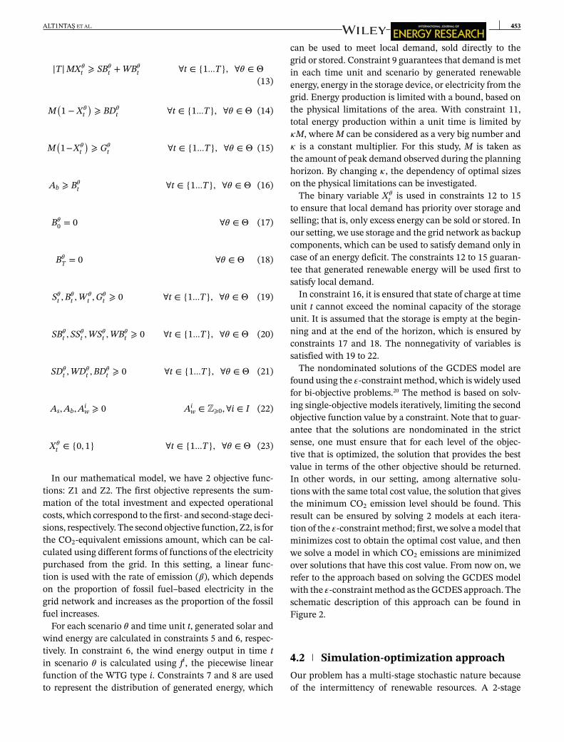
An HRES can be used either to satisfy local demand or tomake a profit by selling green energy to the grid at elevatedprices. In this study, we assume that the decision maker iscarbon sensitive; hence, the priority of the decentralizedsystem is to satisfy local demand using green energy ratherthan feeding energy to the grid to make a profit. If there is asurplus of renewable energy, it can be stored in the storagedevice and/or fed to the grid. We assume that the storagedevice can only store green energy and that this energy canonly be used to satisfy the demand (ie, renewable energycannot be sold to the grid through the storage device; there-fore, we can prioritize renewable energy to be used for localdemand). Fossil fuel–based electricity from the grid will beused as a backup source only when green energy is not ade-quate to meet the demand. A schematic description of thedecentralized system can be found in Figure 1.
Governments impose different incentive policies, suchas feed-in tariff programs, tax deductions, and investmentand operating subsidies, to promote renewable energyinvestments and decrease CO2 emissions.18 We considera setting where a feed-in tariff program is available toinvestors. This program is an incentive policy that aimsto promote renewable energy investments by offeringhigher selling prices for each renewable energy type. Green
FIGURE 1 The grid-connected decentralized energy system
ALT1NTAS ET AL. 451
energy can be sold to the grid for higher prices for a lim-ited time.18 It is expected that feed-in tariff programs willincrease the ratio of clean energy fed to the grid in the longrun. This situation will decrease the carbon emission rateof the electricity bought from the grid. However, in thisstudy, we assume that this improvement is negligible.
The objective of this study is to determine the changein size of the described system with respect to the carbonemission value. To handle the 2 conflicting objectives con-sidered (cost and CO2 emissions), we propose a solutionframework in which we determine the optimal sizing ofthe components and their relations and present a set ofsolutions rather than a single solution. Our solution frame-work is generic, that is, independent of the system scale.Thus, it can be used for demand points of different sizes atdifferent locations.
The decisions to be made in such systems are of 2 types:investment decisions and operational decisions. Invest-ment decisions include sizing decisions for the compo-nents (solar panel area, number of wind turbines, storagesize) and are made at the beginning of the time hori-zon. Operational decisions, on the other hand, are madein each time unit, such as deciding on the amount ofenergy to be stored, purchased, and/or sold. All these deci-sions are to be made considering both cost and emissioncriteria. Note that in addition to being bi-objective, theproblem is stochastic because of the uncertainty of renew-able resources. The decision support system we proposehelps the decision maker to make investment decisions forsuch systems, taking into account the problem's multicri-teria and stochastic natures.
4 SOLUTION APPROACHES
4.1 Bi-objective 2-stage stochasticmixed-integer programming approachIn 2-stage stochastic programs, the decision-making pro-cess is divided into 2 stages, where there are 2 differ-ent types of decision variables: first and second stage.First-stage variables are decided on before the realiza-tion of random parameters. After uncertain events unfold(such as availability of renewable resources), operationaldecisions can be made. The general form of the 2-stagestochastic linear program is given below:
Min cTX + E[Q(X , 𝜉(𝜃))
]s.t AX = b
X ⩾ 0
where Q(X , 𝜉(𝜃)) = Min qTYs.t tX + wY = h
Y ⩾ 0
where X and Y are first- and second-stage variables,respectively. The second-stage problem depends on thedata (q, t,w, h), where some or all elements can be ran-dom. The expectation of Q is taken with regard to theprobability of 𝜉. Randomness in 𝜉 can be incorporatedin 2 ways. The first way uses a continuous probabil-ity distribution. This approach keeps the problem sizesteady, but it may cause nonlinearities and computationaldifficulties.19 The second way is scenario based. In thisapproach, uncertainty is modeled as a union of randomdiscrete events. There are a finite number of possible out-comes with certain probabilities, and the problem sizeincreases enormously depending on the number of out-comes. Let Θ be the number of possible outcomes and p𝜃
be the corresponding occurrence probability of scenario 𝜃.Then, the 2-stage stochastic program with discrete randomevents becomes:
We model our problem as a bi-objective 2-stage stochas-tic mixed-integer program. To be able to model the ran-dom availabilities of resources, we follow a scenario-basedapproach. Renewable energy generation depends onuncertain data such as wind speed and solar irradia-tion, and the sizing decision must be made before suchuncertainties are realized. Once the component sizes ofthe decentralized system are determined, the amount ofrenewable energy generation can be calculated and oper-ational decisions (storing, outsourcing, and meeting localdemand) can be made accordingly. The parameters anddecision variables of our GCDES model are introduced inTables 2 and 3, respectively.
The GCDES decides on the capacity of renewable energygeneration and storage components to be built in the areaof interest by minimizing the annualized total cost andCO2 emissions. Fixed costs (cb, cs, ci
w) represent the cost ofthe renewable resource investment, which includes capi-tal, operation, and maintenance costs. We annualize theseinvestment costs by multiplying each component by itsannualization factor, which is calculated using the equiva-lent annual cost formula considering the discount rate (dr)and the respective lifetime of a component. We show anexample calculation for solar in Formula 1.
𝛼s =dr
1 + (1 − dr)−Ls. (1)
452 ALT1NTAS ET AL.
TABLE 2 Parameters, sets
T Time horizon (t ∈ {1...T})I Set of wind turbine generator (WTG) typesΘ Set of scenarios (𝜃 ∈ Θ)dr Discount ratecb Investment cost of storage unit, $/kWhcs Investment cost of solar panel, $/m2
ciw Investment cost of WTG type i, $/unit
Lb Lifetime of storage unit, yearsLs Lifetime of solar panel, yearsLi
w Lifetime of WTG type i, yearsLFT Duration of feed-in tariff policy, yearsLsystem Duration of the GCDES, years𝛼b Annualization factor for storage unit𝛼s Annualization factor for solar panel𝛼w Annualization factor for wind turbines𝛼ps Annualization factor for sale price of solar energy𝛼pw Annualization factor for sale price of wind energypg Price of electricity purchased from grid (spot price), $/kWhps Elevated sale price of solar energy, $/kWhpw Elevated sale price of wind energy, $/kWhd𝜃
t Local demand in (t, 𝜃), kWhv𝜃t Wind speed in (t, 𝜃), m/sr𝜃t solar irradiation in (t, 𝜃), kW/m2
𝜂s Overall efficiency of solar panel, %𝜂b Storage efficiency, %𝜅 Electricity generation limit multiplierM Maximum unit time demand, kWh𝛽 CO2 Equivalent emission by electricity grid, tonne/kWh
The electricity purchase price (pg) represents the averageretail price of electricity in the market. Governments thatpractise a feed-in tariff policy offer different elevated saleprices (higher than the retail price of electricity) for eachrenewable energy resource to investors.18 This policy hasdifferent prices for each renewable source (pw, ps) and isusually available for a limited amount of time. Therefore,incentivized prices cannot be used throughout the lifespanof the system. After the feed-in tariff expires, green energybecomes available to the market at retail price. Thus, wedistribute the effect of an elevated sale price (ps, pw) acrossthe lifetime of the system. Formula 2 calculates the annual-ization factor for the sale price of solar energy (𝛼ps), whereLFT represents the duration of the feed-in tariff policy. Thesame formula is used to calculate the annualization factorfor the sale price of wind energy (𝛼pw) by replacing (ps)with (pw).
𝛼ps =psLFT + pg(Lsystem − LFT)
psLsystem. (2)
TABLE 3 Decision variables
Ab Size of storage unit, kWhAs Size of solar panels, m2
Aiw Number of WTGs of type i
S𝜃t Electricity generated by solar panels in (t, 𝜃), kWh
SD𝜃t Solar electricity used to satisfy demand in (t, 𝜃), kWh
SB𝜃t Solar electricity used to charge battery in (t, 𝜃), kWh
SS𝜃t Solar electricity sold to grid in (t, 𝜃), kWh
W𝜃t Electricity generated by WTGs in (t, 𝜃), kWh
WD𝜃t Wind electricity used to satisfy demand in (t, 𝜃), kWh
WB𝜃t Wind electricity sent to storage in (t, 𝜃), kWh
WS𝜃t Wind electricity sold to grid in (t, 𝜃), kWh
B𝜃t State of charge at the end of time t in scenario 𝜃, kWh
BD𝜃t Discharge amount in (t, 𝜃), kWh
G𝜃t Amount of electricity supplied from the grid in (t, 𝜃), kWh
X𝜃t 1, if electricity is not purchased from the grid in (t, 𝜃)
0, if electricity is not fed to the grid in (t, 𝜃)
4.1.1 Mathematical model formulation
min Z1 ∶ 𝛼bcbAb + 𝛼scsAs + 𝛼w∑i∈I
ciwAi
w
+ 1|Θ|
∑𝜃∈Θ
∑t∈T
[pgG𝜃
t − 𝛼pspsSS𝜃t − 𝛼pwpwWS𝜃
t] (3)
min Z2 ∶ 𝛽1|Θ|
∑𝜃∈Θ
∑t∈T
G𝜃t (4)
s.t
S𝜃t = 𝜂sr𝜃t As ∀t ∈ {1...T}, ∀𝜃 ∈ Θ (5)
W𝜃t =
∑i∈I
f i(v𝜃t)
Aiw ∀t ∈ {1...T}, ∀𝜃 ∈ Θ (6)
S𝜃t = SS𝜃
t + SD𝜃t + SB𝜃
t ∀t ∈ {1...T}, ∀𝜃 ∈ Θ (7)
W𝜃t = WS𝜃
t +WD𝜃t +WB𝜃
t ∀t ∈ {1...T}, ∀𝜃 ∈ Θ (8)
d𝜃t = SD𝜃
t + WD𝜃t + 𝜂bBD𝜃
t + G𝜃t ∀t ∈ {1...T}, ∀𝜃 ∈ Θ
(9)
B𝜃t = B𝜃
t−1+SB𝜃t +WB𝜃
t −BD𝜃t ∀t ∈ {1...T}, ∀𝜃 ∈ Θ (10)
𝜅M ⩾ S𝜃t + W𝜃
t ∀t ∈ {1...T}, ∀𝜃 ∈ Θ (11)
𝜅MX𝜃t ⩾ SS𝜃
t + WS𝜃t ∀t ∈ {1...T}, ∀𝜃 ∈ Θ (12)
ALT1NTAS ET AL. 453
|T|MX𝜃t ⩾ SB𝜃
t + WB𝜃t ∀t ∈ {1...T}, ∀𝜃 ∈ Θ
(13)
M(1 − X𝜃
t)⩾ BD𝜃
t ∀t ∈ {1...T}, ∀𝜃 ∈ Θ (14)
M(1−X𝜃
t)⩾ G𝜃
t ∀t ∈ {1...T}, ∀𝜃 ∈ Θ (15)
Ab ⩾ B𝜃t ∀t ∈ {1...T}, ∀𝜃 ∈ Θ (16)
B𝜃0 = 0 ∀𝜃 ∈ Θ (17)
B𝜃T = 0 ∀𝜃 ∈ Θ (18)
S𝜃t ,B𝜃
t ,W𝜃t ,G𝜃
t ⩾ 0 ∀t ∈ {1...T}, ∀𝜃 ∈ Θ (19)
SB𝜃t , SS𝜃
t ,WS𝜃t ,WB𝜃
t ⩾ 0 ∀t ∈ {1...T}, ∀𝜃 ∈ Θ (20)
SD𝜃t ,WD𝜃
t ,BD𝜃t ⩾ 0 ∀t ∈ {1...T}, ∀𝜃 ∈ Θ (21)
As,Ab,Aiw ⩾ 0 Ai
w ∈ Z⩾0,∀i ∈ I (22)
X𝜃t ∈ {0, 1} ∀t ∈ {1...T}, ∀𝜃 ∈ Θ (23)
In our mathematical model, we have 2 objective func-tions: Z1 and Z2. The first objective represents the sum-mation of the total investment and expected operationalcosts, which correspond to the first- and second-stage deci-sions, respectively. The second objective function, Z2, is forthe CO2-equivalent emissions amount, which can be cal-culated using different forms of functions of the electricitypurchased from the grid. In this setting, a linear func-tion is used with the rate of emission (𝛽), which dependson the proportion of fossil fuel–based electricity in thegrid network and increases as the proportion of the fossilfuel increases.
For each scenario 𝜃 and time unit t, generated solar andwind energy are calculated in constraints 5 and 6, respec-tively. In constraint 6, the wind energy output in time tin scenario 𝜃 is calculated using fi, the piecewise linearfunction of the WTG type i. Constraints 7 and 8 are usedto represent the distribution of generated energy, which
can be used to meet local demand, sold directly to thegrid or stored. Constraint 9 guarantees that demand is metin each time unit and scenario by generated renewableenergy, energy in the storage device, or electricity from thegrid. Energy production is limited with a bound, based onthe physical limitations of the area. With constraint 11,total energy production within a unit time is limited by𝜅M, where M can be considered as a very big number and𝜅 is a constant multiplier. For this study, M is taken asthe amount of peak demand observed during the planninghorizon. By changing 𝜅, the dependency of optimal sizeson the physical limitations can be investigated.
The binary variable X𝜃t is used in constraints 12 to 15
to ensure that local demand has priority over storage andselling; that is, only excess energy can be sold or stored. Inour setting, we use storage and the grid network as backupcomponents, which can be used to satisfy demand only incase of an energy deficit. The constraints 12 to 15 guaran-tee that generated renewable energy will be used first tosatisfy local demand.
In constraint 16, it is ensured that state of charge at timeunit t cannot exceed the nominal capacity of the storageunit. It is assumed that the storage is empty at the begin-ning and at the end of the horizon, which is ensured byconstraints 17 and 18. The nonnegativity of variables issatisfied with 19 to 22.
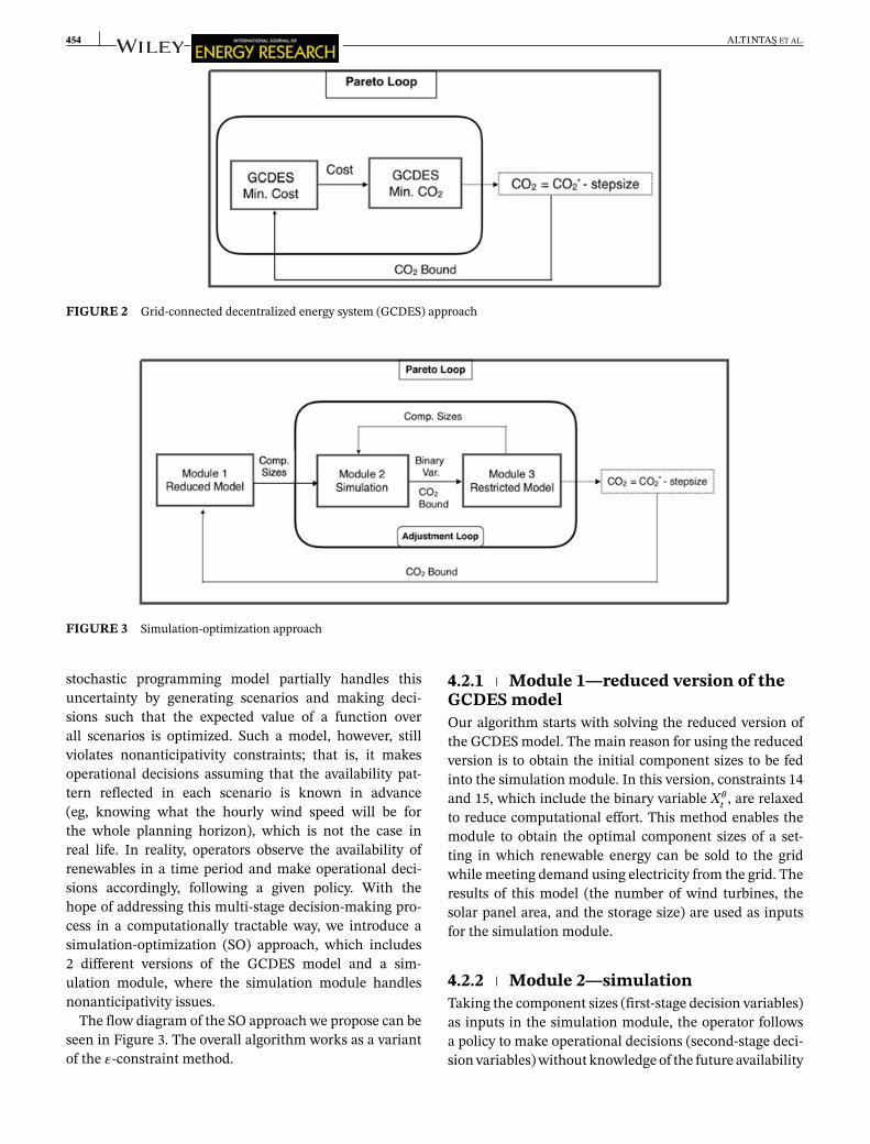
The nondominated solutions of the GCDES model arefound using the 𝜀-constraint method, which is widely usedfor bi-objective problems.20 The method is based on solv-ing single-objective models iteratively, limiting the secondobjective function value by a constraint. Note that to guar-antee that the solutions are nondominated in the strictsense, one must ensure that for each level of the objec-tive that is optimized, the solution that provides the bestvalue in terms of the other objective should be returned.In other words, in our setting, among alternative solu-tions with the same total cost value, the solution that givesthe minimum CO2 emission level should be found. Thisresult can be ensured by solving 2 models at each itera-tion of the 𝜀-constraint method; first, we solve a model thatminimizes cost to obtain the optimal cost value, and thenwe solve a model in which CO2 emissions are minimizedover solutions that have this cost value. From now on, werefer to the approach based on solving the GCDES modelwith the 𝜀-constraint method as the GCDES approach. Theschematic description of this approach can be found inFigure 2.
4.2 Simulation-optimization approachOur problem has a multi-stage stochastic nature becauseof the intermittency of renewable resources. A 2-stage
454 ALT1NTAS ET AL.
FIGURE 2 Grid-connected decentralized energy system (GCDES) approach
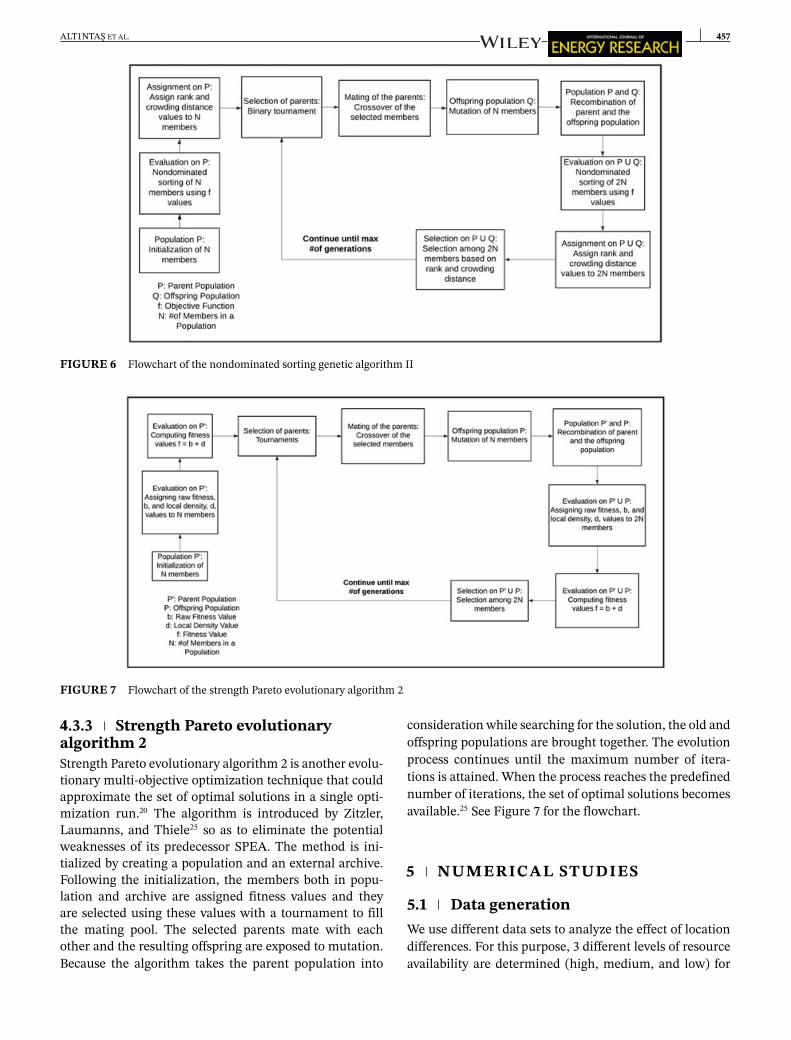
FIGURE 3 Simulation-optimization approach
stochastic programming model partially handles thisuncertainty by generating scenarios and making deci-sions such that the expected value of a function overall scenarios is optimized. Such a model, however, stillviolates nonanticipativity constraints; that is, it makesoperational decisions assuming that the availability pat-tern reflected in each scenario is known in advance(eg, knowing what the hourly wind speed will be forthe whole planning horizon), which is not the case inreal life. In reality, operators observe the availability ofrenewables in a time period and make operational deci-sions accordingly, following a given policy. With thehope of addressing this multi-stage decision-making pro-cess in a computationally tractable way, we introduce asimulation-optimization (SO) approach, which includes2 different versions of the GCDES model and a sim-ulation module, where the simulation module handlesnonanticipativity issues.
The flow diagram of the SO approach we propose can beseen in Figure 3. The overall algorithm works as a variantof the 𝜀-constraint method.
4.2.1 Module 1—reduced version of theGCDES modelOur algorithm starts with solving the reduced version ofthe GCDES model. The main reason for using the reducedversion is to obtain the initial component sizes to be fedinto the simulation module. In this version, constraints 14and 15, which include the binary variable X𝜃
t , are relaxedto reduce computational effort. This method enables themodule to obtain the optimal component sizes of a set-ting in which renewable energy can be sold to the gridwhile meeting demand using electricity from the grid. Theresults of this model (the number of wind turbines, thesolar panel area, and the storage size) are used as inputsfor the simulation module.
4.2.2 Module 2—simulationTaking the component sizes (first-stage decision variables)as inputs in the simulation module, the operator followsa policy to make operational decisions (second-stage deci-sion variables) without knowledge of the future availability
ALT1NTAS ET AL. 455
of wind and solar resources. The policy is designed to pri-oritize renewable sources while meeting local demand,which is in line with the objective of minimizing theCO2 emission value. This module takes the investmentdecisions (the number of wind turbines, the solar panelarea, and the storage size) obtained from the reducedversion of the GCDES model and calculates the renew-able energy generated at each time period of the planninghorizon for each scenario. First, local demand is satisfiedusing a less-profitable renewable energy source, and thenexcess energy is transferred to the storage unit until it isfull. If there is still excess energy, it is sold to the grid.When there is insufficient renewable energy to satisfy localdemand, first, the amount is discharged from the storageunit if possible and then any deficit amount is purchasedfrom the grid. In this way, the simulation module deter-mines whether to sell renewable energy or outsource fossilfuel–based electricity from the grid, which corresponds tothe binary variables in the GCDES model (X𝜃
t ). The result-ing total CO2 emission value and related binary variables(X𝜃
t ) are used as inputs in module 3 (the restricted versionof the GCDES model).
4.2.3 Module 3—restricted version of theGCDES modelIn the restricted version, the output of the simulation mod-ule is used to dictate purchasing/selling decisions. Thesedecisions are conveyed to the model by fixing binary vari-ables (X𝜃
t ) in constraints 14 and 15. Moreover, the total CO2emission value observed in the simulation module is usedto update the CO2 limit in the restricted model. This modelis solved, and the new investment decisions are fed back tothe simulation module, which now applies the policy usingthe new component sizes. In this way, the component sizesand the purchasing/selling decisions can be adjusted itera-tively. This adjustment continues until the decisions made
in modules 2 and 3 are in line with each other, and the(adjustment) loop terminates when the improvement incost is less than 0.1%. Each such loop provides a solutionwith a corresponding cost and CO2 level. To move to thenext (neighbor) solution, we further restrict the CO2 limitby subtracting a predetermined amount (step size) fromthe CO2 level of the latest solution found. A new (Pareto)loop is initiated by solving module 1 with this new CO2limit (see the outer loop in Figure 3).
4.3 Metaheuristic approachesFor the addressed problem, we present metaheuristic algo-rithms that consist of 2 modules as in the SO approach.In the optimization module, existing multi-objective meta-heuristic algorithms are used to obtain a Pareto front andthe simulation module is the same with that of the SOapproach discussed in Section 4.2. These procedures startwith an initial set of solutions with randomly generatedcomponent sizes. Then these solutions are conveyed tothe module 2 so as to perform the simulation. Given anoperation policy and the component sizes, the simulationmodule makes the operational decisions and the objec-tive function values are calculated. The resulting cost andCO2 emission values are returned to the optimization mod-ule. Following the algorithm steps, an approximate Paretofront is generated in the end. The working scheme of theapproach can be found in Figure 4.
As seen in the Figure 4, simulation and optimizationmodules operate in a loop where they provide input foreach other. For the simulation purposes, we resort to thepreviously discussed module 2, while optimized MOPSO(OMOPSO), nondominated sorting genetic algorithm II(NSGA-II), and strength Pareto evolutionary algorithm(SPEA) 2 are employed in the module 1 regarding theoptimization.
FIGURE 4 Metaheuristic approach
456 ALT1NTAS ET AL.
FIGURE 5 Flowchart of the optimized multi-objective particle swarm optimization algorithm
4.3.1 Optimized MOPSOParticle swarm optimization (PSO) algorithm proposed byKennedy and Eberhart21 is one of the popular metaheuris-tic algorithms used in diverse optimization tasks. Thisalgorithm mimics the flocking of birds and tries to find anoptimal solution throughout the search space. At the initialstep of the procedure, a set of solutions called swarms orparticles is generated. As these swarms fly over the feasiblearea, each particle updates its velocity and position accord-ing to a group of equations. These equations consider boththe best solution that particle has found so far and all thebest solutions found by the members of the swarm. In theend, the optimal solution is attained via particle experienceand best global particle.21
Although PSO performs well in a range of optimiza-tion problems, its application is restricted to the sin-gle objective problems.22 Extending the idea of PSO tomulti-objective problems, Coello and Lechuga22 developMOPSO algorithm. The main idea of MOPSO is includ-ing a global repository in which each particle depositsits flight experience after a cycle. Later, this reposi-tory is used by the swarms to select the leader thatguides the flight. Differently from the PSO, the resultis a set of nondominated solutions that are kept in therepository.22
Many algorithms originated from MOPSO can be foundin the literature.23 Although they have the common ideaof selecting the leader from the nondominated particles,the selection process could be different. To compare theseMOPSOs, an experimental study is conducted by Durilloet al.23 Three benchmark problems and performance met-rics are employed so as to make the comparison. Theresults of the experiments indicate that OMOPSO per-forms best in all of the studied problems. Because of itssuperior performance, OMOPSO algorithm is applied to
the present problem, minimizing total cost and CO2 emis-sion simultaneously. The algorithm runs following thesteps outlined in Figure 5.
4.3.2 Nondominated sorting geneticalgorithm IIGenetic algorithms are used for solving a variety of multi-objective optimization problems, thanks to their ability toprovide good solutions in a reasonable amount of time.20
These algorithms work according to the evolutionary prin-ciples in the optimization of both continuous and discretevalued problems. Nondominated sorting genetic algorithmII, one of the genetic algorithms, has been applied to differ-ent multi-objective optimization tasks because of its con-vergence performance.24 The procedure starts with ran-domly generating N members. After the generation, thesemembers are sorted into different nondomination levelsby pairwise comparisons. When the sorting task is com-pleted, each member is assigned 2 attributes, which arelater used in the selection. Having these properties, themembers experience selection and mutation, which causechanges in the member itself.24 In the end, the offspringpopulation of size N is obtained. To store the solutionsfrom the parent population, former and offspring popula-tions are combined. The recently created population with2N members is nondomination sorted. There should be aselection between these nondomination sorted membersso as to maintain the size N. In the selection, previouslyassigned properties are taken into account. This whole pro-cess continues until a predefined number of generationsare reached. At the end of all steps, a Pareto set of solu-tions is obtained.24 Generational loop of the NSGA-II canbe found in Figure 6.
ALT1NTAS ET AL. 457
FIGURE 6 Flowchart of the nondominated sorting genetic algorithm II
FIGURE 7 Flowchart of the strength Pareto evolutionary algorithm 2
4.3.3 Strength Pareto evolutionaryalgorithm 2Strength Pareto evolutionary algorithm 2 is another evolu-tionary multi-objective optimization technique that couldapproximate the set of optimal solutions in a single opti-mization run.20 The algorithm is introduced by Zitzler,Laumanns, and Thiele25 so as to eliminate the potentialweaknesses of its predecessor SPEA. The method is ini-tialized by creating a population and an external archive.Following the initialization, the members both in popu-lation and archive are assigned fitness values and theyare selected using these values with a tournament to fillthe mating pool. The selected parents mate with eachother and the resulting offspring are exposed to mutation.Because the algorithm takes the parent population into
consideration while searching for the solution, the old andoffspring populations are brought together. The evolutionprocess continues until the maximum number of itera-tions is attained. When the process reaches the predefinednumber of iterations, the set of optimal solutions becomesavailable.25 See Figure 7 for the flowchart.
5 NUMERICAL STUDIES
5.1 Data generationWe use different data sets to analyze the effect of locationdifferences. For this purpose, 3 different levels of resourceavailability are determined (high, medium, and low) for
458 ALT1NTAS ET AL.
TABLE 4 Renewable resource availability data
Wind speed (m/s) Solar irradiation (kW/m2)
Data Set Min Mean Max Min Mean MaxHigh 0.21 7.81 29.90 0 0.24 1.09Medium 0.13 5.14 19.35 0 0.17 0.97Low 0.02 3.33 11.92 0 0.08 0.66
FIGURE 8 Solar and wind profiles for medium availability level [Colour figure can be viewed at wileyonlinelibrary.com]
solar and wind energy alike. Solar irradiation and windspeed data are gathered using Hybrid Optimization of Mul-tiple Energy Resources software. Statistics for the differentlevels of resource availability data can be found in Table 4.For example, we represent a place with medium windspeed and medium solar irradiation by generating datawith a mean wind speed value of 5.14 m/s and mean solarirradiation value of 0.17 kW/m2.
To illustrate, wind speed and solar irradiation for 1-yearprofiles for the medium availability level are representedin Figure 8.
For our numerical study, we consider a medium-scaledemand point such as a university campus. To generatean illustrative data set, we obtain 1 month of the hourlyaverage electricity consumption data of Bilkent Universitycampus in Turkey. By preserving the electricity consump-tion characteristics of Bilkent University, hourly consump-tion profiles for 1 year are generated using Hybrid Opti-mization of Multiple Energy Resources software. Bilkent'saverage hourly and monthly electricity consumption canbe found in Figure 9.
Three different wind turbine types with differently ratedpowers are used in the analysis. These turbines have capac-ities of 0.9, 2, and 3 MW. Wind energy generation cal-culations are made based on the respective power curveof each turbine.26 Parameters for the numerical analysisare provided in Table 5. For more information about theparameters and numerical analysis, see Altıntas.27 TheGCDES and SO approaches are implemented in MAT-LAB 9.0 and solved using CPLEX 12.6. The source codesof metaheuristic algorithms written in JAVA environmentare executed.28 All of these solution procedures are run ina computer with Intel Xeon CPU E5-1650 3.6 GHz proces-sor and 32 GB RAM. The resulting times are expressed incentral processing unit (CPU) seconds.
5.2 Comparison of metaheuristicalgorithmsSo as to assess the quality of Pareto fronts obtained bymetaheuristics, performance metrics are introduced inmulti-objective optimization literature. These measures
w $5.49 M 𝜂b 80Lb 10 years r 0.05Ls 30 years 𝜅 2Lw 20 years 𝛽 0.0004836Lsystem 30 years T 8760 hoursLFT 10 years
can be categorized into 3 groups based on their ability todepict a certain aspect of the solution set.29
1. Metrics that assess convergence to the knownPareto-optimal front.
2. Metrics that evaluate spread of the solutions on thePareto-optimal front.
3. Metrics that measure combinations of solutions' con-vergence and spread.
In this study, each Pareto front is evaluated using variousmetrics from the above categories. Because the true Paretofront is unknown, it is not possible to measure the conver-gence truly. Instead, coverage value is computed so as tocompare 2 Pareto sets with each other. Together with thecoverage metric, hypervolume measure from the third cat-egory is employed to assess the convergence and spread ofsolutions simultaneously. In addition to this assessment,
FIGURE 10 Hypervolume measure for a 2-objectiveminimization case [Colour figure can be viewed atwileyonlinelibrary.com]
spacing and maximum spread values are calculated forevaluating the solutions' spread.
Spacing (S): The measure is proposed by Schott30 andhas been used to estimate the diversity of Pareto front.In the formulation, n stands for the number of solu-tions in frontier, di represents the minimum Manhattandistance between a solution i and any other solution,and d is the average distance between 2 solutions. As Sbecomes zero, a more uniformly distributed Pareto frontis attained.
S =
√√√√ 1n − 1
×n∑
i=1(di − d)2. (24)
Maximum spread (MS): Zitzler31 introduces maximumspread metric to measure the spread of a given set. For thismeasure, greater values are preferred because they indi-cate a better spread of the points. The measure is calculatedas follows where ai and bi are 2 solutions in Pareto frontierand n is the number of solutions.
MS =
√√√√ n∑i=1
max(||ai − bi||). (25)
Coverage (C): The coverage metric, suggested by Zitzler,31
is used to determine whether a Pareto front dominatesanother. So as to make the comparison between 2 Paretofronts, A and B, each solution from one front is comparedwith all solutions in the other front. Two points, a and b,are compared with each other at a time using the weaklydominance operator shown as ⪰. The coverage values ofsets A and B are represented by C(A,B) and C(B,A). IfC(A,B) is equal to 1, it means all solutions in the set Bare weakly dominated by A. In the opposite case, whereC(A,B) is 0, none of the points in B is weakly dominated byA. Because there could be interaction between 2 sets, bothdirections should be considered in the calculation.
C(A,B) = |{b ∈ B|∃a ∈ A ∶ a ⪰ b}||B| . (26)
Hypervolume: The hypervolume measure is first pro-posed by Zitzler and Thiele32 as the size of space covered.With change in the name over the time, this metric hasbeen applied for evaluating the Pareto solutions' conver-gence and spread at the same time. For this purpose,the hypervolume quantifies the volume of the dominated
space, which is enclosed with a reference point. Usually,the point in the reference set having the worst-case resultsfor each of the objective is selected, and by adding somedelta value, the reference point is reached. Considering a2-objective minimization problem setting, with objectivefunctions f1(x) and f2(x), the computed area can be seen inFigure 10.33
Given the economic parameters and the data sets, 3well-known algorithms, OMOPSO, NSGA-II, and SPEA2,are tested for a medium solar–medium wind probleminstance with 9 scenarios. To find the parameter config-uration of each algorithm, different generations are tried.By changing the generation count, various sets of opti-mal solutions are obtained. These solutions are comparedbased on some popular performance metrics, and theirvalues are recorded in Tables 6 to 8. So as to providean example for the tuning of the algorithms, OMOPSOalgorithm is selected, and its generation count is arrangedbased on the metric results in Table 6.
All of the performance metric results indicate that 5000and 10 000 evaluations should be preferred over the others.Provided that there is no significant difference between5000 and 10 000 evaluations in terms of the other per-formance measures, the version, which takes less CPUtime, 5000 is chosen. Tunings of the other algorithmsare completed following the same steps here and in theend 5000 generations is accepted as the parameter of the3 algorithms.
Using 5000 generations, statistical analyses are con-ducted. For this purpose, each metaheuristic algorithmis run for 10 times and their results are compared basedon the hypervolume measure. This metric is selectedbecause it evaluates both convergence and spread ofthe solutions. Minimum, mean and maximum valuesof this measure are listed in Table 9. To understandwhich algorithm performs the best, hypothesis test-ing is conducted. While checking if there is a signifi-cant difference between OMOPSO, NSGA-II, and SPEA2,Kruskal-Wallis and Mann-Whitney U tests are applied.34
The results of these tests clearly show that OMOPSO is thebest performing algorithm for the given problem. Whenthe other 2 algorithms are compared with each other,no significant difference is found. Therefore, OMOPSOalgorithm is used for obtaining the set of Pareto solu-tions in our stochastic bi-objective optimization of theGC system.
Performance metric/# of evaluations 500 1000 5000 10 000
Spacing 0.0120 0.0128 0.0039 0.0042Max Spread 10.4554 10.1637 10.2725 10.2664CPU Time (s) 141.44 290.30 1423.75 2930.03
TABLE 8 Performance measure results for nondominated sorting genetic algorithm II algorithm
Performance metric/# of evaluations 500 1000 5000 10 000
Spacing 0.0122 0.0074 0.0072 0.0069Max Spread 9.3381 10.1065 10.0013 10.2081CPU Time (s) 144.83 279.61 1406.53 2935.09
TABLE 9 Hypervolume metric results for algorithms
Algorithm Hypervolume Count Indifferent
Min Median MaxOMOPSO 0.579 0.581 0.582 10 -NSGA2 0.571 0.576 0.578 10 SPEA2SPEA2 0.570 0.578 0.579 10 NSGA2
TABLE 10 Attributes of generated scenarios
Solar irradiation (kW/m2)Scenario 1 Scenario 2 Scenario 3
Level Min Mean Max Min Mean Max Min Mean MaxHigh 0 0.2442 1.1108 0 0.244 1.1412 0 0.2441 1.1354Medium 0 0.1748 0.9987 0 0.1749 1.0029 0 0.1748 0.9916Low 0 0.0835 0.6757 0 0.0835 0.6634 0 0.0835 0.6872
Wind Speed (m/s)Scenario 1 Scenario 2 Scenario 3
Level Min Mean Max Min Mean Max Min Mean MaxHigh 0 7.3669 26.9398 0.0066 7.5248 26.6697 0.0309 7.3283 24.5682Medium 0.0001 4.6157 17.3236 0.0025 4.6938 17.6675 0.0004 4.6461 18.5492Low 0.0019 3.0054 9.6265 0.0048 3.0585 10.6093 0.0014 2.9368 10.7751
5.3 Comparative analysis
In this part, 3 solution methods (GCDES, SO, andOMOPSO) are compared with each other by taking thestochasticity of a location's renewable resources intoconsideration. To handle the stochasticity aspect of theproblem, a scenario-wise approach is used. For solar data,scenarios are formed via perturbation of the profiles shownin Figure 8. Choosing the parameter as 5%, the procedureof Kuznia et al7 is followed in the scenario generation. Forwind data, techniques introduced by Dukes and Palutikof35
and McNerney and Veers36 are used to create the scenar-ios. In the literature, the Weibull distribution is commonlyused to generate synthetic wind speed data.37 In that tech-nique, different states are constructed and wind speedis generated using a Markov transition matrix, which isconstructed using the Weibull distribution. Wind speedvalues are centered around the given mean value, and the
correlation between time units is handled by a decreasingexponential function.
For each of our low, medium, and high solar and windcases, 3 scenarios are generated, and their statistics aregiven in Table 10.
The GCDES, SO, and OMOPSO algorithms are run for9 different locations (combinations of high, medium, andlow resource availability levels) using 9 different scenarios(combinations of 3 solar and 3 wind scenarios), of the dataof which are introduced in Section 5.1. The outputs of thesecomputational experiments can be found in Table 11.
As it is seen among the results, GCDES approach failsto conclude the experiment in a predesignated amountof time for all 9 cases and, hence, delivers only a fewsolutions. On the other hand, SO method provides a satis-factory number of outcomes after the process is completed.The results indicate that OMOPSO algorithm is able toachieve a variety of solutions with less computational
462 ALT1NTAS ET AL.
TAB
LE11
Out
puts
ofth
eG
CD
ES,S
O,a
ndO
MO
PSO
appr
oach
esfo
r9sc
enar
ios
GC
DES
SOO
MO
PSO
Sola
rW
ind
#So
lnSt
artG
P(%
)aEn
dG
P(%
)bG
ap(%
)c#
Soln
Star
tGP
(%)a
End
GP
(%)b
#So
lnSt
artG
P(%
)aEn
dG
P(%
)b
Leve
lLe
vel
Soln
sTi
me
(s)
Soln
sTi
me
(s)
Soln
sTi
me
(s)
Hig
hH
igh
118
000e
100.
010
0.0
42.7
713
085
35.9
4.7
121
1468
37.9
5.4
Med
ium
Hig
h1
1800
0e10
0.0
100.
042
.78
1249
137
.91.
534
714
6337
.91.
6Lo
wH
igh
118
000e
100.
010
0.0
42.7
783
2337
.95.
116
514
3837
.95.
4H
igh
Med
ium
234
110e
100.
095
.07.
34
3319
53.5
35.5
397
1400
100.
036
.5M
ediu
mM
ediu
m2
4615
6e10
0.0
95.0
246.
311
3604
310
0.0
48.7
1136
1367
100.
049
.6Lo
wM
ediu
m2
2904
2e10
0.0
95.0
4.8
949
073
100.
052
.733
614
1210
0.0
53.2
Hig
hLo
w2
3321
0e10
0.0
95.0
0.06
439
6453
.537
.142
214
6410
0.0
36.4
Med
ium
Low
571
996e
100.
080
.0N
Ad
1143
1010
0.0
48.9
703
1452
100.
048
.7Lo
wLo
w5
6544
6e10
0.0
75.0
42.2
939
1210
0.0
58.7
995
1460
100.
059
.7a
Perc
enta
geof
dem
and
satis
fied
byth
egr
idof
the
first
Pare
toso
lutio
nfo
und.
b Perc
enta
geof
dem
and
satis
fied
byth
egr
idof
the
last
Pare
toso
lutio
nfo
und.
c The
optim
ality
gap
ofth
ela
stso
lutio
n.d N
oin
tege
rsol
utio
nis
foun
dfo
rthe
last
itera
tion.
e Indi
cate
stha
tthe
com
puta
tiona
ltim
elim
itha
sbee
nre
ache
dfo
rthe
last
solu
tion
(18
000
s).
TAB
LE12
Perf
orm
ance
met
ricso
fthe
GC
DES
,SO
,and
OM
OPS
Oap
proa
ches
for9
scen
ario
s
GC
DES
SOO
MO
PSO
Sola
rW
ind
SM
SC
(SO
,C
(OM
OPS
O,
SM
SC
(GC
DES
,C
(OM
OPS
O,
SM
SC
(GC
DES
,C
(SO
,Le
vel
Leve
lG
CD
ES)(
%)
GC
DES
)(%
)SO
)(%
)SO
)(%
)O
MO
PSO
)(%
)O
MO
PSO
)(%
)
Hig
hH
igh
Inf
-Inf
100.
010
0.0
0.3
2.9
0.0
0.0
0.03
511
.90.
014
.9M
ediu
mH
igh
Inf
-Inf
100.
010
0.0
0.3
3.1
0.0
12.5
0.00
520
.40.
05.
8Lo
wH
igh
Inf
-Inf
100.
010
0.0
0.3
2.9
0.0
14.3
0.00
813
.70.
013
.3H
igh
Med
ium
0.0
1.7
0.0
100.
00.
12.
20.
025
.00.
005
21.3
0.0
0.3
Med
ium
Med
ium
0.0
1.7
0.0
100.
00.
13.
49.
190
.90.
002
34.5
0.0
0.0
Low
Med
ium
0.0
1.7
50.0
100.
00.
23.
111
.177
.80.
008
18.5
0.0
0.0
Hig
hLo
w0.
01.
70.
010
0.0
0.1
2.2
0.0
0.0
0.00
422
.00.
03.
8M
ediu
mLo
w0.
02.
40.
060
.00.
13.
59.
154
.50.
004
26.8
0.0
1.4
Low
Low
0.4
2.4
20.0
100.
00.
13.
111
.166
.70.
002
31.8
0.0
0.6
ALT1NTAS ET AL. 463
effort compared with the other approaches. Although thistable gives valuable insights about the performances, it isnecessary to conclude the comparison by looking at theperformance measures.
With the 3 metrics implemented, performances of theall approaches can be seen in Table 12. It should be notedthat infinity values are recorded because GCDES methodfinds only one solution in that cases because of time limit.Although this algorithm has S values as 0 in some set-tings, the overall performance of the method can be notedas poor when MS and C numbers are taken into account.While comparing SO and OMOPSO, it is clear that thereare significant differences between the numerical results.For the S measure, OMOPSO has numbers that are almostone-tenth of the SO. A similar ratio is observed among the
FIGURE 11 Nine-scenario Pareto of the grid-connecteddecentralized energy system (GCDES), simulation-optimization(SO), and optimized multi-objective particle swarm optimization(OMOPSO) approaches for the medium solar–medium wind case
MS values. Despite high weakly domination ratios in somecases, OMOPSO performs better in terms of the C metricas well. The results can be seen graphically in Figure 11.
Because of the mediocre performance of the GCDESin 9 scenarios, we now reduce our solution approachesto SO and OMOPSO while working with the scenariosin which demand uncertainty is included. Using mediumsolar–medium wind case and by generating 3 and 5 sce-narios for demand, the number of scenarios is increasedto 27 and 125, respectively. The outcomes of this studycan be seen in Table 13. By looking at this table, we canconclude that OMOPSO returns a diverse set of solutionswhich performs better in all of the metrics in a shorteramount of time.
5.4 Sensitivity analysisA sensitivity analysis is also conducted to determine theeffect of the key parameters on the investment size of thesystem components for the medium solar–medium windresource level. For this analysis, we first bound the CO2level such that the total amount of energy purchased fromthe grid will not exceed 60% of the total demand, andsolve the problem with our SO and OMOPSO approaches.We investigate the effects of the investment costs of solar,wind, and storage as well as the selling prices of solarand wind energy. For each cost parameter, we halve anddouble the value (while keeping all other parameters attheir base levels). For selling prices, we double the val-ues to see the effect of an increase in the feed-in tariffpolicy. The results are summarized in Tables 14 and 15.Note that in this problem instance, storing energy is notcost efficient even when the investment cost of storageis halved.
TABLE 13 Outputs of the SO and OMOPSO approaches for 27 to 125 scenarios
SO OMOPSOSoln S MS C(OMOPSO, SO) (%) #Solns Soln S MS C(SO, OMOPSO) (%)
Motivated by the interest in shifting from fossil fuel–basedcentralized energy systems to decentralized renewableenergy systems to decrease emissions, we consider the siz-ing problem of a GC decentralized system. This system isa hybrid decentralized system that depends on solar andwind energy generation backed up with a storage. Ourmain aim is to provide insights for decision makers aboutthe optimal scale of the decentralized system they plan toinvest in. The optimal sizing decision problem includes 2important aspects, stochasticity (uncertainty of renewableresources) and a multi-objective structure (having con-cerns for multiple criteria such as cost and emissions).In our study, we consider these 2 aspects elaborately byassuming that the decision maker is responsive to cost andenvironment (carbon emission) alike and by modeling theproblem as a stochastic problem, using random resourceavailabilities.
We provide a mathematical programming formulation.We then discuss alternative solution approaches thatinclude a simulation-optimization approach and meta-heuristic algorithms. We first model the problem asa bi-objective 2-stage stochastic mixed-integer program.This model has 2 objective functions: minimizing theannualized system cost as well as the amount of emit-ted CO2-equivalent gases while satisfying local demand.Nondominated solutions of this model are generated usingthe 𝜀-constraint method. This model determines optimalcomponent sizes for a predetermined CO2 emission limitand also determines optimal operational decisions, such asselling, outsourcing, and storing energy in each time unit.Further, we develop a simulation-optimization method,which approaches the multi-stage stochastic nature of theproblem in a more realistic way. Preserving the simulationmodule of this newly introduced method, 3 well-knownmetaheuristic algorithms are investigated additionally.
A numerical analysis of all methods is performed formultiple-scenario cases. The outputs of the study indicatethat the GCDES approach cannot find the whole Paretoset in a reasonable time. Simulation-optimization is better
at returning various solutions, however, is outperformedby OMOPSO, which returns better quality solutions inless time.
As future research, this study can be extended in mul-tiple directions. One extension would be to considermore objectives, such as reliability and social acceptance.Interaction among these objectives can provide valuableinsights for the decision maker. Another research directionworth exploring is considering ways to increase the uncer-tainty in the problem. We envisage a potential extensionin this direction: One can assume that price parametersare also uncertain. As the number of uncertain param-eters increases, the models will become more realistic,yet harder to solve. This situation provides the opportu-nity to investigate methodologies to tackle the computa-tional challenges as well as to demonstrate the value ofstochasticity in such cases. Moreover, one can also consideralternative multi-objective metaheuristic approaches such asmulti-objective gravitational search and multi-objective har-mony search in the optimization module of our algorithm.
ORCID
Özlem Karsu http://orcid.org/0000-0002-9926-2021
REFERENCES1. World Alliance for Decentralized Energy. Policy to promote de.
2. Tina G, Gagliano S. Probabilistic analysis of weather datafor a hybrid solar/wind energy system. Int J Energy Res.2011;35(3):221-232.
3. Kaundinya DP, Balachandra P, Ravindranath NH.Grid-connected versus stand-alone energy systems for decen-tralized power—a review of literature. Renew SustainableEnergy Rev. 2009;13(8):2041-2050.
4. Jebaraj S, Iniyan S. A review of energy models. Renew sustainableenergy rev. 2006;10(4):281-311.
5. Hiremath RB, Shikha S, Ravindranath NH. Decentralizedenergy planning; modeling and application—a review. RenewSustainable Energy Rev. 2007;11(5):729-752.
6. Ardakani FJ, Riahy G, Abedi M. Optimal sizing of agrid-connected hybrid system for north-west of iran-case study.Prague, Czech Republic; 2010:29-32.
7. Kuznia L, Zeng B, Centeno G, Miao Z. Stochastic optimiza-tion for power system configuration with renewable energy inremote areas. Ann Oper Res. 2013;210(1):411-432.
8. Gonzalez A, Riba J-R, Rius A, Puig R. Optimal sizing of ahybrid grid-connected photovoltaic and wind power system.Appl Energy. 2015;154:752-762.
9. Bortolini M, Gamberi M, Graziani A. Technical and economicdesign of photovoltaic and battery energy storage system. EnergyConvers Manage. 2014;86:81-92.
10. Chedid R, Rahman S. Unit sizing and control of hybridwind-solar power systems. IEEE T Energy Conver.1997;12(1):79-85.
11. Wang L, Singh C. PSO-based multi-criteria optimum design ofa grid-connected hybrid power system with multiple renewablesources of energy. In: 2007 IEEE Swarm Intelligence Sympo-sium, Honolulu, HI, USA; 2007:250-257.
12. Perera ATD, Attalage RA, Perera KKCK. Optimal design of a gridconnected hybrid electrical energy system using evolutionarycomputation. In: 2013 IEEE 8th International Conference onIndustrial and Information Systems, Peradeniya, Sri Lanka;2013:12-17.
13. Sharafi M, ElMekkawy TY, Bibeau EL. Optimal design of hybridrenewable energy systems in buildings with low to high renew-able energy ratio. Renew Energy. 2015;83:1026-1042.
14. Sharafi M, ElMekkawy TY. Stochastic optimization of hybridrenewable energy systems using sampling average method.Renew Sustainable Energy Rev. 2015;52:1668-1679.
15. Sharafi M, ElMekkawy TY. A dynamic MOPSO algorithm formultiobjective optimal design of hybrid renewable energy sys-tems. Int J Energy Res. 2014;38(15):1949-1963.
16. Powell WB, George A, Simao H, Scott W, Lamont A, Stew-art J. Smart: a stochastic multiscale model for the analysis ofenergy resources, technology, and policy. INFORMS J Comput.2012;24(4):665-682.
17. Kocaman AS, Abad C, Troy TJ, Huh WT, Modi V. A stochasticmodel for a macroscale hybrid renewable energy system. RenewSustainable Energy Rev. 2016;54:688-703.
18. K International. Taxes and incentives for renewable energy.https://assets.kpmg.com/content/dam/kpmg/pdf/2015/09/taxes-and-incentives-2015-web-v2.pdf, Accessed June 2016;2015.
19. Birge JR, Louveaux F. Introduction to Stochastic Programming.New York, NY: Springer New York; 2011.
20. Deb K. Multi-Objective Optimization using Evolutionary Algo-rithms, Vol. 16: In Multi-objective Evolutionary Optimisationfor Product Design and Manufacturing. Wang L., Ng AHC andDeb K. eds. London: Springer London; 2001:3-34.
21. Eberhart R, Kennedy J. A new optimizer using particle swarmtheory. In: Proceedings of the Sixth International Symposiumon Micro Machine and Human Science, 1995. MHS'95, Nagoya,Japan, Japan; 1995:39-43.
22. Coello CAC, Lechuga MS. MOPSO: A proposal for multipleobjective particle swarm optimization. In: Proceedings of the2002 Congress on Evolutionary Computation, 2002. CEC '02, Vol.2. Honolulu, HI, USA, 2002:1051-1056.
23. Durillo AJ, García-Nieto J, Nebro AJ, Coello CAC, Luna F,Alba E. Multi-objective particle swarm optimizers: An experi-mental comparison. In: Evolutionary Multi-Criterion Optimiza-tion, Vol. 5467, Ehrgott, M. Fonseca, CM Gandibleux X,Hao J-K, and Sevaux M, Eds. Berlin, Heidelberg: Springer BerlinHeidelberg; 2009:495-509.
24. Deb K, Pratap A, Agarwal S, Meyarivan TAMT. A fast and eli-tist multiobjective genetic algorithm: NSGA-II. IEEE T EvolutComput. 2002;6(2):182-197.
25. Zitzler E, Laumanns M, Thiele L. SPEA2: Improving thestrength pareto evolutionary algorithm; 2001.
26. ENERCON. Enercon product overview. http://www.enercon.de/fileadmin/Redakteur/Medien-Portal/broschueren/pdf/en/ENERCON_Produkt_en_06_2015.pdf, Accessed June 2016;2015.
27. Altıntas O. Bi-objective optimization of grid-connected decen-tralized energy systems. Ms Thesis: Bilkent University; 2016.
28. Source code. https://github.com/MOEAFramework/MOEAFramework/releases/download/v2.12/MOEAFramework-2.12-Source.tar.gz, Accessed May 2017.
29. Deb K. Multi-objective optimisation using evolutionary algo-rithms: An introduction; 2011.
30. Schott JR. Fault tolerant design using single and multicriteriagenetic algorithm optimization [techincal report]. DTIC Docu-ment; 1995.
31. Zitzler E. Evolutionary algorithms for multiobjective optimiza-tion: Methods and applications [PhD thesis]. Switzerland: ETHZurich; 1999.
32. Zitzler E, Thiele L. Multiobjective evolutionary algorithms: acomparative case study and the strength Pareto approach. IEEET Evolut Comput. 1999;3(4):257-271.
33. Hadka D. Beginner's Guide to the MOEA Framework. 2.8 edition.CreateSpace Independent Publishing Platform, 2016.
34. Examples. http://moeaframework.org/examples.htmlexample2, Accessed May 2017.
35. Dukes MDG, Palutikof JP. Estimation of extreme windspeeds with very long return periods. J Appl Meteorol.1995;34(9):1950-1961.
36. McNerney GM, Veers PS. A Markov Method for SimulatingNon-Gaussian Wind Speed Time Series: Wind America, Albu-querque, NM: Sandia National Labs., Albuquerque, NM (USA);1985.
37. Conradsen K, Nielsen LB, Prahm LP. Review of Weibull statis-tics for estimation of wind speed distributions. J Clim ApplMeteorol. 1984;23(8):1173-1183.
How to cite this article: Altintas O, Okten B,Karsu O, Kocaman AS. Bi-objective optimiza-tion of a grid-connected decentralized energysystem. Int J Energy Res. 2018;42:447–465.https://doi.org/10.1002/er.3813