Page 1
1
Bias Correction of Satellite-Based Rainfall Estimates for Modeling
Flash Floods in Semi-Arid regions: Application to Karpuz River,
Turkey
Mohamed Saber 1, 2, 3, Koray K. Yilmaz2
1Geology Department, Faculty of Science, Assiut University, Assiut 71516, Egypt 5 2Department of Geological Engineering, Middle East Technical University, 06800, Ankara, Turkey
3Water Resources Research Center, DPRI, Kyoto University, Goka-sho, Uji City, Kyoto 611-0011, Japan;
Correspondence to: Mohamed Saber ([email protected] )
Abstract: This study investigates the utility of gauge-corrected satellite-based rainfall estimates in simulating flash floods at
Karpuz River - a semi-arid basin in Turkey. Global Satellite Mapping of Precipitation (GSMaP) product was evaluated with 10
the rain gauge network at monthly and daily time-scales considering various time periods and rainfall rate thresholds. Statistical
analysis indicated that GSMaP shows acceptable linear correlation coefficient with rain gauges however suffers from
significant underestimation bias. A rainfall rate threshold of 1 mm/month was the best choice to improve the match between
GSMaP and rain gauges implying that appropriate threshold selection is critically important for the bias correction.
Multiplicative bias correction was applied to GSMaP data using the bias factors calculated between GSMaP and observed 15
rainfall. Hydrological River Basin Environmental Assessment Model (Hydro-BEAM) was used to simulate flash floods at the
hourly time scale driven by the corrected GSMaP rainfall data. The model parameters were calibrated for flash flood events
during October-December 2007 and then validated for flash flood events during October-December 2009. The results show
that the simulated surface runoff hydrographs reasonably coincide with the observed hydrographs.
Keywords: Flash floods modeling; semi-arid regions; bias correction; GSMaP; Antalya; Turkey 20
Nat. Hazards Earth Syst. Sci. Discuss., doi:10.5194/nhess-2016-339, 2016Manuscript under review for journal Nat. Hazards Earth Syst. Sci.Published: 11 November 2016c© Author(s) 2016. CC-BY 3.0 License.
Page 2
2
1. Introduction
Spatio-temporal variation of rainfall is important to understand the hydrological and climatic characteristics of watersheds, as
well as for planning effective water management and hazard mitigation strategies for water-related disasters such as flash
floods and droughts. The influence of rainfall representation on the modelling of the hydrologic response is expected to depend
on complex interactions between the rainfall space-time variability, the variability of the catchment soil and landscape 5
properties, and the spatial scale (i.e. catchment area) of the problem (Obled et al., 1994; Woods and Sivapalan, 1999; Bell and
Moore, 2000; Smith et al., 2004). River hydrograph forecasts are highly dependent upon the input rainfall data used.
Streamflow in arid and semi-arid regions is characterized by rapid response to intense rainfall events. Such events frequently
have a high degree of spatial variability. Coupled with poorly gauged rainfall data this situation sets a fundamental limit on
the capacity of the rainfall-runoff models to reproduce the observed flow (Wheater et al., 2008), thus hampering prediction 10
efforts. It has been widely stated that the major limitation of the development of arid-zone hydrology is the lack of high quality
observations (McMahon and Greene, 1979; Pilgrim et al., 1988).
Accurate temporal knowledge of global precipitation is definitely important for understanding the multi-scale interactions
among weather, climate and ecological systems, as well as for improving the ability to manage the available water resources
and predict high-impact weather events including hurricanes, floods, droughts and landslides (Hou et al., 2008). Rain gauge 15
observations yield relatively accurate point measurements of precipitation but are not well distributed and not available over
most oceanic and unpopulated land areas (Xie and Arkin, 1996; Petty and Krajewski, 1996). In particular, the arid and semi-
arid regions are suffering from poor rain gauge network coverage and the lack of continuous observations, especially at the
hourly timescale, which will be consequently a challenge for the flash floods mitigation efforts. Therefore, algorithms
developed for bias correction of the satellite-based rainfall data are desperately needed in such regions. 20
The combination of satellite measurements and gauge data is in great need to enhance spatio-temporal rainfall estimation (Chiu
et al., 2006a). Global satellite-based rainfall datasets are becoming increasingly available in different spatial and temporal
resolutions and freely accessible. For example, widely used global rainfall datasets include; the Global Satellite Mapping of
Nat. Hazards Earth Syst. Sci. Discuss., doi:10.5194/nhess-2016-339, 2016Manuscript under review for journal Nat. Hazards Earth Syst. Sci.Published: 11 November 2016c© Author(s) 2016. CC-BY 3.0 License.
Page 3
3
Precipitation (GSMaP) (Okamoto et al., 2005); (Ushio et al., 2009), Precipitation Estimation from Remotely Sensed
Information using Artificial Neural Networks (PERSIANN) (Hsu et al., 1999; Sorooshian et al., 2000), Climate Prediction
Center (CPC) Morphing technique (CMORPH) (Joyce et al., 2004; Xie, 2013) Tropical Rainfall Measuring Mission (TRMM)
Multi-satellite Precipitation Analysis (TMPA) (Huffman et al., 2010).
Recent decades are marked by increasing flash flood hazards in many regions over the world due to increase in the frequency 5
of flash floods as well as rapid urbanization. The term ‘flash flood’ identifies a rapid hydrological response, with water levels
reaching a peak within less than one hour to a few hours after the onset of the generating rain event (Creutin et al., 2013;
Collier, 2007; Younis et al., 2008). The most important challenge to model implementation and calibration to simulate flash
floods in semi-arid and arid regions is the lack of necessary observational networks of both rainfall and discharge.
Responsible factors for the short duration of the flash flood include intense rains that persist on an area for a few hours, steep 10
slope, impermeable surfaces, and sudden release of impounded water over small basins (Georgakakos, 1986).
Flood occurrences are complex since they depend on interactions between many geological and morphological characteristics
of the basins, including rock types, elevation, slope, sediment transport, and flood plain area. Moreover, hydrological
phenomena, such as rainfall, runoff, evaporation, and surface and groundwater storage (Farquharson et al., 1992; Flerchinger
and Cooley, 2000; Nouh, 2006) affect floods. According to (Few et al., 2004), each flood acquires some particular and inherent 15
characteristics of the occurrence locality, such as flow velocity and height, duration, and rate of water-level rise.
In many countries and regions of the world, flash floods are the most costly natural hazards in terms of both loss of human
lives and material damage (Fattorelli et al., 1999; Creutin et al., 2013). In particular, arid and semi-arid regions have become
more vulnerable to flash floods than before possibly due to the global climate change and rapid population growth. The main
obstacle to study flash floods is clearly the lack of reliable observations in most of the flash flood prone basins. Furthermore, 20
the danger also comes from the rarity of the phenomenon, which demands new observation strategies, as well as new
forecasting methodologies.
Nat. Hazards Earth Syst. Sci. Discuss., doi:10.5194/nhess-2016-339, 2016Manuscript under review for journal Nat. Hazards Earth Syst. Sci.Published: 11 November 2016c© Author(s) 2016. CC-BY 3.0 License.
Page 4
4
Various problems associated with forecasting flash floods caused by convective storms over semi-arid basins have been studied
by (Michaud and Sorooshian, 1994). Rapidly increasing availability of good quality weather radar observations is greatly
expanding our ability to measure and monitor rainfall distribution at the space and time scales which characterize the flash-
flood events (Borga et al., 2007). Moreover, some hydrological approaches and understanding of runoff characteristics in arid
environment have been developed by (Saber et al., 2010b; Saber et al., 2013), and a method for estimating flash flood peak 5
discharge, hydrograph, and volume has been presented by (Koutroulis and Tsanis, 2010). Hence an integrated and
comprehensive research regarding flash flood modeling and forecasting approaches as well as mitigation strategies are
desperately needed in semi-arid and arid regions.
A suite of models is available to represent rainfall-runoff relationships, but they have limitations in the hydrologic parameters
that are used to describe the rainfall–runoff process in semi-arid and arid systems (Wheater et al., 1993). It has been widely 10
stated that the major limitation of the development of arid-zone hydrology is the lack of high quality observations (McMahon
and Greene, 1979; Pilgrim et al., 1988). Thus, implementation of a hydrological model driven by locally corrected satellite-
based rainfall estimates could be useful in overcoming majority of the problems in simulating flash floods, thus potentially
serve as a tool for hazard mitigation and sustainable development of the target basin.
A comparative study has been done (Saber, 2010; Saber et al., 2013) between GSMaP and the Global Precipitation Climatology 15
Center (GPCC) in the arid and semi-arid regions over the globe to characterize the GSMaP product bias as compared to
observed GPCC product. Additional analysis using the local raingauge network at a semi-arid region will be considered in this
research for further validation of GSMaP product. Consequently, the forecasting models driven by the bias-corrected satellite-
based rainfall datasets are expected to be more powerful and reliable. This study aims to compare GSMaP product with the
gauge-based precipitation estimates in Karpuz River located in Antalya, Turkey in an effort to devise a correction methodology 20
for the GSMaP product to drive a hydrological model for flash-flood simulation. Due to rapid occurrence of flash floods at
sub-daily time scales generally hourly spatio-temporal rainfall data is used for flash flood simulation studies. Thus, satellite-
based rainfall data at the hourly timescale with continuous availability in time provides an alternative to ground-based
Nat. Hazards Earth Syst. Sci. Discuss., doi:10.5194/nhess-2016-339, 2016Manuscript under review for journal Nat. Hazards Earth Syst. Sci.Published: 11 November 2016c© Author(s) 2016. CC-BY 3.0 License.
Page 5
5
observations for flash flood simulation studies. The paper consists of two main parts. First, data comparison and the procedure
for correction of Satellite-based rainfall data (GSMaP) is introduced. Second, flash flood modeling through a hydrological
model with calibrated and validated parameters for Karpuz River - a semi-arid basin in Antalya, Turkey is provided.
2 Study Area and Datasets
The study area is the Karpuz River Basin located to the west of the city of Antalya situated in the Mediterranean region of 5
Turkey. The study area lies between 30.50E-32.50E longitude bands and 36.00N-37.50N Latitude bands with a total area of
about 1920 km2, where the land data pixels were only considered for the analysis (Fig. 1).
Figure 1: The study area selected for the comparison between GSMaP and rain gauge data.
Antalya
Manavgat
Alanya
Mediterranean Sea
Nat. Hazards Earth Syst. Sci. Discuss., doi:10.5194/nhess-2016-339, 2016Manuscript under review for journal Nat. Hazards Earth Syst. Sci.Published: 11 November 2016c© Author(s) 2016. CC-BY 3.0 License.
Page 6
6
Global Satellite Remote Sensing Datasets of GSMaP were compared and validated with rain gauge-based precipitation data in
the study area. Daily precipitation data from five meteorological stations located in the study area were obtained from the
General Directorate of Meteorology and used to validate GSMaP data. The rain gauge data spans different time periods (Table
1), therefore an overlapping time period from 2007 to 2013 was selected. GSMaP products are provided at two different spatial 5
scales; 0.1° x 0.1° and 0.25° x 0.25° degree grids, and two temporal scales (hourly, daily). There also exist different processed
data as listed in Table 2. Hourly GSMaP data product having 0.1° x 0.1° grids were used in this study. The time stamps of both
GSMaP and rain gauge data were matched to enable comparison.
Table 1. Selected rain gauges around the study area 10
Station
Name
Station ID Start Date End date Latitude Longitude Elevation
Antalya 17300 1965 2015 36.91667 30.8 50
Gazipasa 17974 1970 2015 36.26667 32.31667 21
Manavgat 17954 1965 2015 36.7833 31.4333 38
Alanya 17310 1965 2015 36.55 31.9833 5.88
ibradi 27 2007 2015 37.0969 31.5976 1036
Table 2. GSMaP data products used in the analysis (Last access, March 1, 2016)
Data
Products
ftp Spatio-temporal
resolution
Available data
Standard
gauges (v5)
ftp://hokusai.eorc.jaxa.jp/standard_gau
ge/v5/hourly/
0.1° x 0.1°,
Hourly
2000/03-2010/11
reanalysis
gauge (v6)
ftp://hokusai.eorc.jaxa.jp/reanalysis_g
auge/v6/gauge_hr/
0.1° x 0.1°,
Hourly
2011/01-2014/02
Real time ftp://hokusai.eorc.jaxa.jp/realtime/arch
ive/
0.1° x 0.1°,
Hourly
2008/10-2016/02
Nat. Hazards Earth Syst. Sci. Discuss., doi:10.5194/nhess-2016-339, 2016Manuscript under review for journal Nat. Hazards Earth Syst. Sci.Published: 11 November 2016c© Author(s) 2016. CC-BY 3.0 License.
Page 7
7
3. Comparison of GSMaP product with Rain gauges
The main objective of this comparison was to validate GSMaP data products with the available rain gauge data in the vicinity
of the Karpuz River Basin (Antalya, Turkey), in order to contribute to the enhancement of hydrological forecasting of flash
floods in semi-arid regions. The time period for the evaluation was selected as the years 2007 through 2013 based on the
availability of the rain gauges. Statistical analysis was performed for the GSMaP data in order to estimate the data bias and 5
to examine its feasibility to be used for the flash floods simulations. The gauge-based rainfall data were interpolated to a 0.1°
x 0.1° resolution grid to be consistent with the GSMaP product resolution using the automated Thiessen polygons (Han and
Bray, 2006), based on the distance formula:
𝐷 = √(𝑥𝑖 − 𝑥𝑗)2 + (𝑦𝑖 − 𝑦𝑗)2 (1)
where D is the distance between the rain gauge and the target pixel (x, y), i refers to the number of station and j for the pixel 10
number. In the procedure, the pixels are assigned the same rainfall rate with the nearest station.
Monthly rainfall averages over the target area were calculated both for hourly GSMaP data, and daily rain gauges with the
same spatial resolution. The analysis for comparison consisted of various scenarios including different time series and different
rainfall thresholds, areal average and pixel to pixel comparisons. Four thresholds (0 mm, 1 mm, 5 mm, and 10 mm) were 15
examined in order to conduct the comparison between rain gauges and GSMaP rainfalls data properly. Statistical parameters
considered in the comparison include: (i) Bias (Eq. 2) the ratio of spatially averaged monthly rainfall obtained from GSMaP
and rain gauges, (ii) Percent bias (PBIAS; Eq. 3) measures the average tendency of the satellite data to the rain gauge estimates
with a best value of zero. Negative values indicate an overestimation by GSMaP, while positive values indicate an
underestimation. (iii) The Nash-Sutcliffe efficiency (Eq. 4) is a normalized statistic that determines the relative magnitude of 20
the residual variance (“noise”) compared to the measured data variance (“information”) (Nash and Sutcliffe, 1970) . NSE
indicates how well the Satellite data matches the gauge data and it ranges between negative infinity and unity; the latter
indicating a perfect agreement. (iv) Coefficient of determination (R2) describe the degree of collinearity between satellite-
Nat. Hazards Earth Syst. Sci. Discuss., doi:10.5194/nhess-2016-339, 2016Manuscript under review for journal Nat. Hazards Earth Syst. Sci.Published: 11 November 2016c© Author(s) 2016. CC-BY 3.0 License.
Page 8
8
based rainfall and gauge-based rainfall. R2 ranges between 0 and 1, with higher values indicating less error variance, and
typically values greater than 0.5 are considered acceptable (Santhi et al., 2001;Van Liew et al., 2003).
𝐵𝑖𝑎𝑠 𝑅𝑎𝑡𝑖𝑜 = 𝐺𝑆𝑀𝑎𝑝
𝑅𝑎𝑖𝑛 𝑔𝑎𝑢𝑔𝑒 (2)
𝑃𝐵𝐼𝐴𝑆 = ∑ (𝑃𝐺
𝑖 −𝑃𝑆𝑖 )𝑛
𝑖=1
∑ 𝑃𝐺𝑖𝑛
𝑖=1
∗ 100 (3)
𝑁𝑆𝐸 = 1 −∑ (𝑃𝐺
𝑖 −𝑃𝑆𝑖 )2𝑛
𝑖=1
∑ (𝑃𝐺𝑖 −𝑃𝑆
𝑚𝑒𝑎𝑛)2𝑛𝑖=1
∗ 100 (4) 5
Where 𝑃𝐺𝑖 is the gauge precipitation values at time i, 𝑃𝑆
𝑖 is the Satellite precipitation values
The results of the statistical analysis, as summarized in Table 3, show that monthly rainfall estimates derived from GSMaP
data are linearly correlated with the rain gauges but significant underestimation of bias is evident. It can also be seen that the
bias magnitude is slightly changing as a function of season (monthly complete time series, April-September, or October to
March), as well as the rainfall threshold (0 mm, 1 mm, 5 mm, and 10 mm) as shown in Table . Scatter plots and hyetographs 10
provided in Figs 2, 3, 4, and 5 show a reasonable and acceptable linear correlation but with an underestimated bias in GSMaP
data in most of the discussed cases, especially for the September-April time period. The total average bias factors for the
monthly data comparison indicate underestimation for 1mm threshold case with values 0.78, 0.50, and 0.98 for the three time
periods, namely monthly complete time series, October–March and April-September, respectively (Table 3). We found that
the best reasonable correlation recorded in case of 1mm threshold is for the time period of April-September. Also, the best 15
PBias value also corresponds to the same threshold and time period, implying that the underestimation bias is higher in the
rainy season. The statistical analysis show that both 1mm and 5 mm thresholds are better than the 0mm and 10 mm thresholds.
This situation might be due to the fact that 0mm threshold include all the pixels in the analysis whereas 10 mm threshold
excluding most of the pixels. The GSMaP data was corrected using the bias ratio of 1 mm threshold case, which in turn used
to drive the hydrological model for effective flash floods simulation. 20
Nat. Hazards Earth Syst. Sci. Discuss., doi:10.5194/nhess-2016-339, 2016Manuscript under review for journal Nat. Hazards Earth Syst. Sci.Published: 11 November 2016c© Author(s) 2016. CC-BY 3.0 License.
Page 9
9
Table 3. Statistical analysis results based on four thresholds (0.0, 1, 5, and 10 mm).
Time
period
Parameter Threshold
0.0 mm 1 mm 5 mm 10 mm
2007-2013
(Complete
time series)
Bias 0.46 0.78 0.72 0.31
R2 0.79 0.8 0.85 0.76
NSE 0.3 0.52 0.61 0.25
PBias 69.8 48.17 42.26 77.57
2007-2013
(Oct- Mar)
Bias 0.29 0.50 0.66 0.22
R2 0.74 0.74 0.76 0.7
NSE -0.57 0.082 0.29 -0.61
PBias 73.5 54.18 44.54 79.3
2007-2013
(Apr- Sept)
Bias 0.68 0.98 0.77 0.49
R2 0.79 0.79 0.82 0.69
NSE 0.44 0.78 0.76 0.27
PBias 48.6 13.49 27.5 65.77
5
(a)
(b)
Figure 2: (a) Hyetograph, (b) scatter plot for the monthly precipitation comparison between GSMaP and rain gauges (threshold=
0.0 mm).
0
100
200
300
400
500
600
700
Pre
cip
ita
tio
n (
mm
/mo
nth
)
Time (Monthly)
Gauges and GSMaP (2007-2013)
Gauges GSMaP
y = 0.2379x + 7.1052
R² = 0.7948
0
100
200
300
400
500
600
700
0 100 200 300 400 500 600 700
GS
Ma
P
Gauges
Gauges and GSMaP (2007-2013)
Gauges GSMaP Linear (Gauges GSMaP)
Nat. Hazards Earth Syst. Sci. Discuss., doi:10.5194/nhess-2016-339, 2016Manuscript under review for journal Nat. Hazards Earth Syst. Sci.Published: 11 November 2016c© Author(s) 2016. CC-BY 3.0 License.
Page 10
10
(a)
(b)
Figure 3: (a) Hyetograph, (b) scatter plot for the monthly precipitation comparison between GSMaP and rain gauges (threshold =
1 mm).
(a)
(b)
Figure 4: (a) Hyetograph, (b) scatter plot for the monthly precipitation comparison between GSMaP and rain gauges (threshold= 5
mm). 5
(a)
(b)
Figure 5: (a) Hyetograph, (b) scatter plot for the monthly precipitation comparison between GSMaP and rain gauges (threshold=
10 mm).
0
100
200
300
400
500
600
700
Pre
cip
ita
tio
n (
mm
/mo
nth
)
Time (Monthly)
Gauges and GSMaP (2007-2013)
Gauges GSMaP
y = 0.4163x + 11.208
R² = 0.7963
0
100
200
300
400
500
600
0 100 200 300 400 500 600 700
GS
MaP
Gauges
Gauges and GSMaP (2007-2013)
Gauges GSMaP Linear (Gauges GSMaP)
0
100
200
300
400
500
600
Pre
cip
ita
tio
n (
mm
/mo
nth
)
Time (Monthly)
Gauges and GSMaP (2007-2013)
Gauges GSMaP
y = 0.4808x + 9.3071
R² = 0.846
0
100
200
300
400
500
600
0 100 200 300 400 500 600
GS
MaP
Gauges
Gauges and GSMaP (2007-2013)
Gauges GSMaP Linear (Gauges GSMaP)
0
100
200
300
400
500
600
700
Pre
cip
ita
tio
n (
mm
/mo
nth
)
Time (Monthly)
Gauges and GSMaP (2007-2013)
Gauges GSMaP
y = 0.2049x + 1.9134
R² = 0.7582
0
100
200
300
400
500
600
0 100 200 300 400 500 600
GS
MaP
Gauges
Gauges and GSMaP (2007-2013)
Gauges GSMaP Linear (Gauges GSMaP)
Nat. Hazards Earth Syst. Sci. Discuss., doi:10.5194/nhess-2016-339, 2016Manuscript under review for journal Nat. Hazards Earth Syst. Sci.Published: 11 November 2016c© Author(s) 2016. CC-BY 3.0 License.
Page 11
11
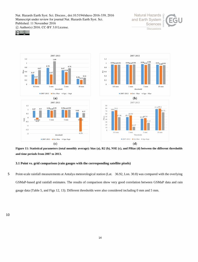
Focusing on the total monthly average precipitation for the 2007-2013 time period (Table 4), the analysis show that the bias
and PBias are slightly changed for each precipitation threshold and time period compared to the previous case (Table 3).
Correlation coefficient and NSE exhibit a significant enhancement for total rainfall average estimates derived from GSMaP
data. Scatter plots and hyetographs (Figs 6, 7, 8, and 9) show a reasonable and acceptable linear correlation but with a 5
significant underestimation bias in GSMaP data in most of the discussed cases, especially for the September-April time period.
Table 4 Statistical analysis based on four thresholds (0.0, 1, 5, 10 mm), in case of the total monthly average precipitation for the
2007-2013 time period.
Time
period Parameter
Threshold
0.0 mm 1 mm 5 mm 10 mm
2007-2013
(all time
series)
Bias 0.47 0.78 0.67 0.26
R2 0.94 0.94 0.96 0.93
NSE 0.87 0.98 0.99 0.68
PBias 69.8 48.17 42.26 77.57
2007-2013
(Oct.-
Mar.)
Bias 0.27 0.47 0.58 0.21
R2 0.92 0.92 0.92 0.88
NSE -0.21 0.89 0.95 -1.73
PBias 73.50 54.18 44.54 79.30
2007-2013
(Apr.-
Sept.)
Bias 0.67 1.09 0.76 0.31
R2 0.93 0.94 0.98 0.91
NSE 0.90 0.99 0.99 0.57
PBias 47.98 12.37 27.17 65.75
10
Nat. Hazards Earth Syst. Sci. Discuss., doi:10.5194/nhess-2016-339, 2016Manuscript under review for journal Nat. Hazards Earth Syst. Sci.Published: 11 November 2016c© Author(s) 2016. CC-BY 3.0 License.
Page 12
12
(a)
(b)
Figure 6: (a) Hyetograph, (b) scatter plot for the total monthly average precipitation comparison between GSMaP and rain gauges
(threshold= 0 mm).
(a)
(b)
Figure 7: (a) Hyetograph, (b) scatter plot for the total monthly average precipitation comparison between GSMaP and rain gauges
(threshold= 1 mm).
(a)
(b)
Figure 8: (a) Hyetograph, (b) scatter plot for the total monthly average precipitation comparison between GSMaP and rain gauges 5
(threshold= 5 mm).
0
50
100
150
200
250
300
350
1 2 3 4 5 6 7 8 9 10 11 12
Rai
nfa
ll (
mm
/mo
nth
)
Months
2007-2013
Gauges GSMaP
y = 0.2252x + 8.5059
R² = 0.9363
0
50
100
150
200
250
300
0 50 100 150 200 250 300 350
GS
MaP
Gauges
2007-2013
GSMaP Linear (GSMaP)
0
50
100
150
200
250
300
350
1 2 3 4 5 6 7 8 9 10 11 12
Rai
nfa
ll (
mm
/month
)
Months
2007-2013
Gauges GSMaP
y = 0.3948x + 13.573
R² = 0.9389
0
50
100
150
200
250
300
0 50 100 150 200 250 300 350
GS
MaP
Gauges
2007-2013
GSMaP Linear (GSMaP)
0
50
100
150
200
250
300
1 2 3 4 5 6 7 8 9 10 11 12
Rai
nfa
ll (
mm
/mo
nth
)
Months
2007-2013
Gauges GSMaP
y = 0.5025x + 7.2104
R² = 0.9637
0
50
100
150
200
250
300
0 50 100 150 200 250 300
GS
MaP
Gauges
2007-2013
GSMaP Linear (GSMaP)
Nat. Hazards Earth Syst. Sci. Discuss., doi:10.5194/nhess-2016-339, 2016Manuscript under review for journal Nat. Hazards Earth Syst. Sci.Published: 11 November 2016c© Author(s) 2016. CC-BY 3.0 License.
Page 13
13
(a)
(b)
Figure 9: (a) Hyetograph, (b) scatter plot for the total monthly average precipitation comparison between GSMaP and rain gauges
(threshold= 10 mm).
Based on the statistical analysis R2, Bias, NSE (Figs 10, 11), we found that R2 varies from 0.7 to 0.98 revealing that GSMaP
shows good linear correlation with rain gauges. Bias and PBias parameters indicate that GSMaP data show underestimation 5
bias in all cases. NSE parameter confirms that 1 mm and 5 mm thresholds are the best compared to the other two thresholds.
(a)
(b)
(c)
(d)
Figure 10: Statistical parameters (monthly): bias (a), R2 (b), NSE (c), and PBias (d) between the different thresholds and time periods
from 2007 to 2013.
0
50
100
150
200
250
300
350
1 2 3 4 5 6 7 8 9 10 11 12
Rai
nfa
ll (
mm
/mo
nth
)
Months
2007-2013
Gauges GSMaP
y = 0.1914x + 3.2443
R² = 0.9336
0
50
100
150
200
250
300
0 50 100 150 200 250 300 350
GS
MaP
Gauges
2007-2013
GSMaP Linear (GSMaP)
0.46
0.780.72
0.310.29
0.5
0.66
0.22
0.68
0.98
0.77
0.49
0
0.2
0.4
0.6
0.8
1
1.2
0.0 mm 1 mm 5 mm 10 mm
Bia
s
threshold
2007-2013
2007-2013 Oct.-Mar Apr. - Sept
0.79 0.80.85
0.760.74 0.74 0.760.7
0.79 0.79 0.82
0.69
0
0.2
0.4
0.6
0.8
1
1.2
0.0 mm 1 mm 5 mm 10 mm
R2
threshold
2007-2013
2007-2013 Oct - Mar Apr - Mar
0.3
0.520.61
0.25
-0.57
0.082
0.29
-0.61
0.44
0.78 0.76
0.27
-0.8
-0.6
-0.4
-0.2
0
0.2
0.4
0.6
0.8
1
0.0 mm 1 mm 5 mm 10 mm
NS
E
threshold
2007-2013
2007-2013 Oct-Mar Apr-Sept
69.8
48.1742.26
77.5773.5
54.18
44.54
79.3
48.6
13.49
27.5
65.77
0.0 mm 1 mm 5 mm 10 mm
0
10
20
30
40
50
60
70
80
90
Thresholds
PB
ias
2007-2013
2007-2013 Oct-Mar Apr-Sept
Nat. Hazards Earth Syst. Sci. Discuss., doi:10.5194/nhess-2016-339, 2016Manuscript under review for journal Nat. Hazards Earth Syst. Sci.Published: 11 November 2016c© Author(s) 2016. CC-BY 3.0 License.
Page 14
14
(a)
(b)
(c)
(d)
Figure 11: Statistical parameters (total monthly average): bias (a), R2 (b), NSE (c), and PBias (d) between the different thresholds
and time periods from 2007 to 2013.
3.1 Point vs. grid comparison (rain gauges with the corresponding satellite pixels)
Point-scale rainfall measurements at Antalya meteorological station (Lat. 36.92, Lon. 30.8) was compared with the overlying 5
GSMaP-based grid rainfall estimates. The results of comparison show very good correlation between GSMaP data and rain
gauge data (Table 5, and Figs 12, 13). Different thresholds were also considered including 0 mm and 5 mm.
10
0.47
0.78
0.67
0.260.27
0.47
0.58
0.21
0.67
1.09
0.76
0.31
0
0.2
0.4
0.6
0.8
1
1.2
0.0 mm 1 mm 5 mm 10 mm
Bia
s
threshold
2007-2013
2007-2013 Oct.-Mar Apr. - Sept
0.94 0.94 0.96 0.930.92 0.92 0.920.88
0.93 0.940.98
0.91
0
0.2
0.4
0.6
0.8
1
1.2
0.0 mm 1 mm 5 mm 10 mm
R2
threshold
2007-2013
2007-2013 Oct - Mar Apr - Mar
0.870.98 0.99
0.68
-0.21
0.89 0.95
-1.73
0.9 0.99 0.99
0.57
-2
-1.5
-1
-0.5
0
0.5
1
1.5
0.0 mm 1 mm 5 mm 10 mm
NS
E
threshold
2007-2013
2007-2013 Oct-Mar Apr-Sept
69.8
48.1742.26
77.5773.5
54.18
44.54
79.3
47.98
12.37
27.17
65.75
0.0 mm 1 mm 5 mm 10 mm
0
10
20
30
40
50
60
70
80
90
Thresholds
PB
ias
2007-2013
2007-2013 Oct-Mar Apr-Sept
Nat. Hazards Earth Syst. Sci. Discuss., doi:10.5194/nhess-2016-339, 2016Manuscript under review for journal Nat. Hazards Earth Syst. Sci.Published: 11 November 2016c© Author(s) 2016. CC-BY 3.0 License.
Page 15
15
Table 5 Statistical analysis based on two thresholds (0.0 and 5mm), in case of point to grid comparisons (Antalya station vs. overlying
GSMaP grid).
Time
period Parameter
Threshold
0.0 mm 5 mm
2007-2013
(all time
series)
Bias 0.99 0.89
R2 0.93 0.92
NSE 0.99 1.00
PBias 16.76 21.57
(a)
(b)
Figure 12: Comparison of point-scale (Antalya station) and grid-scale (GSMaP) mean monthly rainfall using (a) bar chart and (b)
scatterplot (threshold= 0.0 mm). 5
(a)
(b)
Figure 13. Comparison of point-scale (Antalya station) and grid-scale (GSMaP) mean monthly rainfall using (a) bar chart and (b)
scatterplot (threshold= 0.0 mm). (threshold= 5 mm).
0
50
100
150
200
250
1 2 3 4 5 6 7 8 9 10 11 12
Rai
nfa
ll (
mm
/month
)
Months
2007-2013
Antalya Gauge GSMaP
y = 0.7009x + 9.6367
R² = 0.9276
0
50
100
150
200
250
300
0 50 100 150 200 250
GS
MaP
Antalya Gauge
2007-2013
GSMaP Linear (GSMaP)
0
50
100
150
200
250
1 2 3 4 5 6 7 8 9 10 11 12
Rai
nfa
ll (
mm
/mo
nth
)
Months
2007-2013
Antalya Gauge GSMaP
y = 0.6858x + 6.7732
R² = 0.9221
0
50
100
150
200
250
300
0 50 100 150 200 250
GS
MaP
Antalya Gauge
2007-2013
GSMaP Linear (GSMaP)
Nat. Hazards Earth Syst. Sci. Discuss., doi:10.5194/nhess-2016-339, 2016Manuscript under review for journal Nat. Hazards Earth Syst. Sci.Published: 11 November 2016c© Author(s) 2016. CC-BY 3.0 License.
Page 16
16
The different scenarios that we have discussed show that GSMaP and rain gauges show good linear correlation but significant
underestimation bias persist in GSMaP estimates which depend on the seasons and the selected rainfall thresholds. Therefore,
in order to select the appropriate threshold bias results for the GSMaP data correction, we calculated the number of daily
rainfall occurrences above each threshold at different locations (Fig. 14). This analysis focusing on the number of daily
occurrences of above-threshold rainfall for GSMaP and gauges for the whole basins and selected rain gauge stations indicate 5
that threshold value of 1 mm is the best choice for the bias correction between both GSMaP and rain gauges at all stations.
The counting of 10 mm thresholds is not a good option as it excludes most of the rainy days and most of the pixels. Also, 0
mm threshold is considering most of the pixels and days but the problem is that the difference between the two products is too
large -the number of days in GSMaP is higher than those of rain gauges about 20% for the whole daily time series at all
stations. Therefore, the best choice based on this analysis as well as the previous statistical analysis is 1mm threshold because 10
it is exhibiting reasonable daily rainfall occurrence and also the difference between days of GSMaP and rain gauges is not
remarkable - approximately about 2% difference in all cases. Another interesting issue was found in the difference between
the three stations. In case of 5mm and 10 mm thresholds, GSMaP shows underestimated numbers of days at the three stations,
but at Ibradi rain gauge station where the elevation is 1036 m, the difference is more significant compared with the other two
stations at low elevations. For instance, at Ibradi rain gauge, the difference is 141 days, but at Antalya rain gauge the difference 15
is only 8 days. This result implies that the GSMaP product has a more tendency to underestimate rainfall at high elevations
compared to low elevations. This may be due to the snow effect, as stated by (Derin and Yilmaz, 2014) that there are major
challenges to satellite-based precipitation estimation algorithms over complex topography such as those related to orographic
precipitation and precipitation estimation over cold surfaces. For instance, their analysis at the daily time scale revealed that
the CMORPH product suffered from daily precipitation detection problems specifically in the cold season and the windward 20
region, this might be due to the surface snow and ice screening procedure embedded in the algorithm (Joyce et al., 2004) .
Nat. Hazards Earth Syst. Sci. Discuss., doi:10.5194/nhess-2016-339, 2016Manuscript under review for journal Nat. Hazards Earth Syst. Sci.Published: 11 November 2016c© Author(s) 2016. CC-BY 3.0 License.
Page 17
17
Figure 14: Number of rainy days above selected threshold for (a) the whole basin, (b) Antalya rain gauge station (Elevation: 50 m),
(c) Gazipasa rain gauge station (Elevation: 21 m), and (d) Ibradi rain gauge station (Elevation: 1036 m).
The important finding here is that for bias correction of the satellite based data, it is recommended to select the appropriate
threshold for the bias correction. The second finding is that GSMaP data is showing an underestimation bias in all the discussed 5
cases, however it is showing good linear correlations with rain gauge data. The third issue is that GSMaP data shows an
elevation dependent bias. The bias factors estimated from this analysis were used for the correction of GSMaP data in order to
use for the flash floods simulation in the second part of the study.
528
359311
243160
1021
441358
248152
0
200
400
600
800
1000
1200
thr_GT=0 thr_GT=1 thr_GT=2 thr=5 thr=10
Day
nu
mb
ers
Threshold (mm/day)
Antalya
Gauges GSMaP
119997
8692678135
61807
46155
205328
10409881456
50467
28236
0
50000
100000
150000
200000
250000
thr_GT=0 thr_GT=1 thr_GT=2 thr=5 thr=10
Me
sh n
um
be
rs
Threshold (mm/day)
The whole target area
Gauges GSMaP
526418 371
286203
1146
474403
285184
0
200
400
600
800
1000
1200
1400
thr_GT=0 thr_GT=1 thr_GT=2 thr=5 thr=10
Day
nu
mb
ers
Threshold (mm/day)
Gazipasa
Gauges GSMaP
757
543 493392
311
1076
595
462
289170
0
200
400
600
800
1000
1200
thr_GT=0 thr_GT=1 thr_GT=2 thr=5 thr=10
Da
y n
um
be
rs
Threshold (mm/day)
Ibradi
Gauges GSMaP(c) (d)
(a) (b)
Nat. Hazards Earth Syst. Sci. Discuss., doi:10.5194/nhess-2016-339, 2016Manuscript under review for journal Nat. Hazards Earth Syst. Sci.Published: 11 November 2016c© Author(s) 2016. CC-BY 3.0 License.
Page 18
18
3.2 Bias Correction and Distribution Maps of Rainfall over the Target Area
We compared the satellite data with the rain gauges data in order to correct the GSMaP data which are required for the
simulation as hourly input rainfall data. As we have discussed in the previous sections, daily precipitation data from five rain
gauges were obtained from General Directorate of Meteorology for the study area around Karpuz River basin. GSMaP data
were compared and validated using the rain gauges data. The available rain gauges data was available from 2007 to 2013. 5
Afterwards, the calculated bias factors (Eq. 2) from this comparison were used to correct the hourly GSMaP data product to
be used effectively for the flash floods applications. We found that 1 mm threshold is the most appropriate one for bias
correction. Then, GSMaP data were multiplied by the calculated factor in order to correct the data (Eq. 5).
𝐺𝑆𝑀𝑎𝑃𝑐𝑜𝑟𝑟(𝑃(𝑥,𝑦), 𝑇𝑖) =𝐺𝑆𝑀𝑎𝑃(𝑃(𝑥,𝑦), 𝑇𝑖)
𝐵𝑖𝑎𝑠 𝐹𝑎𝑐𝑡𝑜𝑟(𝑇𝑖) (5)
Where GSMaPcorr(P(x,y), Ti) is the corrected GSMaP data at Pixel P(x,y) and hourly time Ti , and GSMaP(P(x,y), Ti) is 10
GRMaP data before correctionsFrom the distribution maps (Fig. 15) of both rain gauges and GSMaP, we found that GSMaP
rainfall data underestimated the rainfall compared to rain gauges, and after the bias correction procedure, GSMap rainfall
improves however, and there is still some differences in the spatial variability of rainfall estimated by rain gauges and GSMaP.
Nat. Hazards Earth Syst. Sci. Discuss., doi:10.5194/nhess-2016-339, 2016Manuscript under review for journal Nat. Hazards Earth Syst. Sci.Published: 11 November 2016c© Author(s) 2016. CC-BY 3.0 License.
Page 19
19
Figure 15:
Distribution maps of daily rainfall data: 2007-12-05, (a) rain gauges, (c) GSMaP, and (e) corrected GSMaP, and 2007-12-07, (b) rain
gauges, (d) GSMaP, and (f) corrected GSMaP.
(a) (b)
(c) (d)
(e) (f)
Nat. Hazards Earth Syst. Sci. Discuss., doi:10.5194/nhess-2016-339, 2016Manuscript under review for journal Nat. Hazards Earth Syst. Sci.Published: 11 November 2016c© Author(s) 2016. CC-BY 3.0 License.
Page 20
20
4 Flash Floods Modeling at Karpuz River
This section analyzes the utility of bias-corrected satellite-based precipitation estimates (GSMaP) for flash floods simulation
in Karpuz River Basin.
4.1 Study Basin
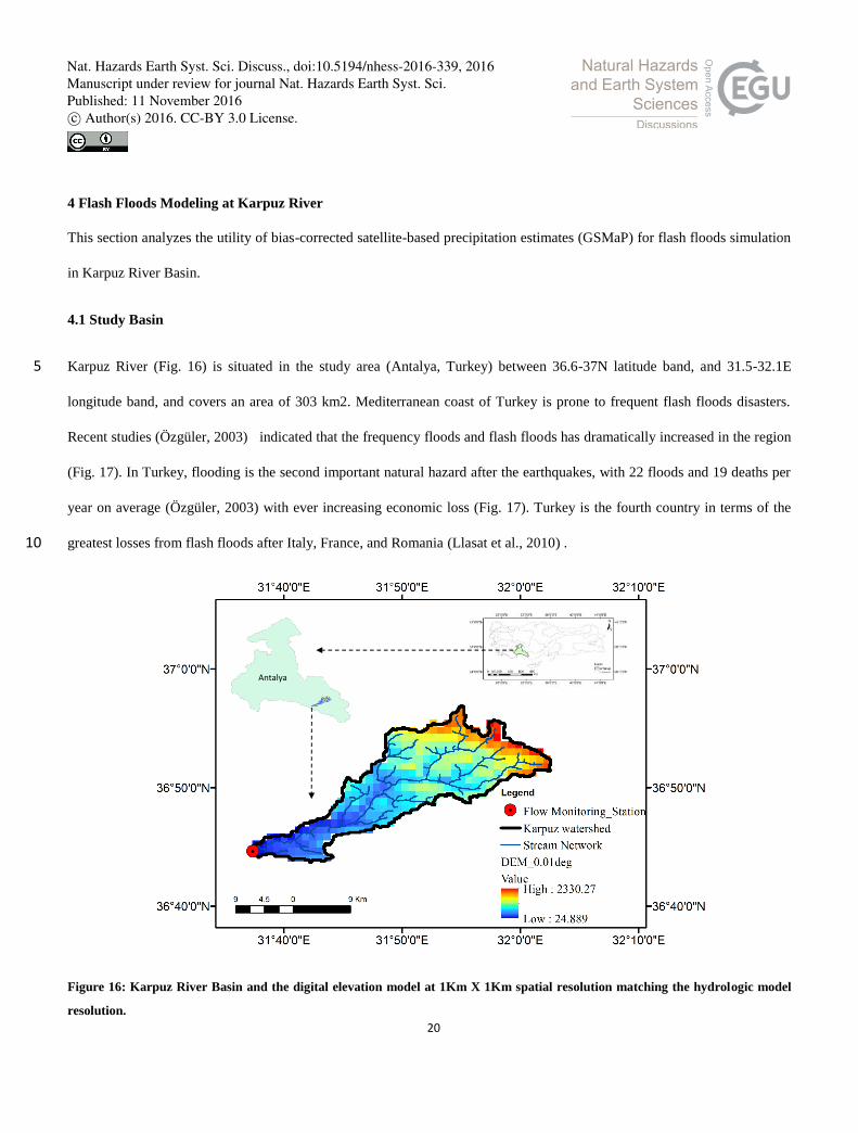
Karpuz River (Fig. 16) is situated in the study area (Antalya, Turkey) between 36.6-37N latitude band, and 31.5-32.1E 5
longitude band, and covers an area of 303 km2. Mediterranean coast of Turkey is prone to frequent flash floods disasters.
Recent studies (Özgüler, 2003) indicated that the frequency floods and flash floods has dramatically increased in the region
(Fig. 17). In Turkey, flooding is the second important natural hazard after the earthquakes, with 22 floods and 19 deaths per
year on average (Özgüler, 2003) with ever increasing economic loss (Fig. 17). Turkey is the fourth country in terms of the
greatest losses from flash floods after Italy, France, and Romania (Llasat et al., 2010) . 10
Figure 16: Karpuz River Basin and the digital elevation model at 1Km X 1Km spatial resolution matching the hydrologic model
resolution.
Antalya
Nat. Hazards Earth Syst. Sci. Discuss., doi:10.5194/nhess-2016-339, 2016Manuscript under review for journal Nat. Hazards Earth Syst. Sci.Published: 11 November 2016c© Author(s) 2016. CC-BY 3.0 License.
Page 21
21
Figure 17: (a) the number of floods in last decade and (b) flood-induced monetary loses in Turkey (Özgüler, 2003) .
4.2 Model Description 5
Hydrological River Basin Environmental Assessment Model (Hydro-BEAM) was selected to simulate the flash flood events
in the study basin. Hydro-BEAM (Fig. 18) is a physically-based distributed hydrological model originally developed (Kojiri
et al., 1998). Hydro-BEAM model has been adopted and implemented in the arid regions by (Saber et al., 2010a; Saber, 2010;
Saber et al., 2013) . The components of the Hydro-BEAM model utilized in this study include a GIS interface for data input
and visualization, surface runoff and stream routing modeling based on the kinematic wave approximation, the initial and 10
transmission losses modeling is estimated via the Curve Number approach (SCS, 1997) and Walter’s equation (Walters, 1990)
respectively, and groundwater modeling based on the linear storage model. However, understanding of hydrological process
resulting in flash floods is hampered by the observational difficulties. In this study, various remotely sensed datasets was used
as input to the hydrological model. Hydro-BEAM is a distributed model consisting of horizontal spatial discretization the scale
of which could be adjusted based on the basin size. Vertically, each pixel is represented by a combination of one surface layer 15
and three subsurface layers (Fig. 18). The surface and subsurface layers are named as A, B, C and D. A-Layer and the river
channel is governed by the kinematic wave model for the overland flow calculation and the layers C and D (subsurface layers)
are modeled using the linear storage model.
(a) (b)
Nat. Hazards Earth Syst. Sci. Discuss., doi:10.5194/nhess-2016-339, 2016Manuscript under review for journal Nat. Hazards Earth Syst. Sci.Published: 11 November 2016c© Author(s) 2016. CC-BY 3.0 License.
Page 22
22
Figure 18: Conceptual model of Hydrological River Basin Environmental Assessment Model (Hydro-BEAM)
4.3 Model Setup
The implementation of the Hydro-BEAM model consist of three main parts, namely, watershed characterization, climatic data 5
preparation, and the main Hydro-BEAM model code. The details of the data processing and model components utilized in this
study are shown in (Fig. 19).
Initial model setup was performed using spatial characteristics of the study basin such as elevation, flow direction, basin
boundary, river channel, land use and spatial grid resolution. ASTER Global Digital Elevation Model (Tachikawa et al.,
2011) having 30m spatial resolution was used to determine the river network and to delineate the watershed boundary. Global 10
Land Cover Characterization (GLCC) dataset (USGS) having a 1km2 resolution was used to identify and extract the land
use distribution of the study basin. GLCC land use data consisted of 24 land use classes. Due to limitations of the Hydro-
BEAM model, 24 land use classes were reclassified into five classes based on the hydrologic characteristics. The resulting five
land use classes include forests, agricultural field, Shrub lands, urban and water.
Waste water
surface runoff
Precipitation
infiltration
Evapo-transpiration
Recovery flow
River flow
GW runoff
A layer
D layer
C layer
B layer
Modeled cell
Initial losses
Transmission losses Wadi System
(1km, 2km, …etc)
Waste water
surface runoff
Precipitation
infiltration
Evapo-transpiration
Recovery flow
River flow
GW runoff
A layer
D layer
C layer
B layer
Modeled cell
Initial losses
Transmission losses Wadi System
(1km, 2km, …etc)
Nat. Hazards Earth Syst. Sci. Discuss., doi:10.5194/nhess-2016-339, 2016Manuscript under review for journal Nat. Hazards Earth Syst. Sci.Published: 11 November 2016c© Author(s) 2016. CC-BY 3.0 License.
Page 23
23
Climate data input is one of the most important factors for hydrological models. Therefore, spatio-temporal distribution of
rainfall and evaporation are needed. Hourly satellite-based GSMaP rainfall data bias corrected following the methodology
described in Section 2.1was used as input to the model. In the procedure, calculated bias for the daily timescale was assumed
to be also valid at the hourly time scale.
Thornthwaite method was adopted to calculate daily mean potential evapotranspiration for each grid because of its simplicity 5
and data availability. This method only requires mean air temperature and duration of possible sunshine for each grid as
meteorological input. Thorntwaite method was applied with the following equations (6-9):
E𝑃 = 0.553D0(10𝑇𝑖/𝐽)𝑎 (6)
𝑎 = 0.000000675𝐽3 − 0.0000771𝐽2 + 0.01792J + 0.049293 (7)
𝐽 = ∑(𝑇𝑖/5)1.514
12
𝑖=1
(8) 10
𝐸𝑎 = 𝑀. 𝐸𝑃 (9)
where Ep is the daily-averaged potential evapotranspiration in i-th month (mmd-1), Do is the possible sunshine duration
(h/12h), J is the heat index, Ti is the a monthly-averaged temperature in i-th month, Ea is the daily-averaged actual
evapotranspiration in i-th month (mmd-1), and M is a evapotranspiration coefficient (reduction coefficient, vapor effective 15
parameter).
Next, main Hydro-BEAM model calculates the streamflow discharge using the kinematic wave model and linear storage
model.
Nat. Hazards Earth Syst. Sci. Discuss., doi:10.5194/nhess-2016-339, 2016Manuscript under review for journal Nat. Hazards Earth Syst. Sci.Published: 11 November 2016c© Author(s) 2016. CC-BY 3.0 License.
Page 24
24
Figure 19: Flow chart of data processing and calculations in Hydro-BEAM.
4 Flash floods Simulation at Karpuz River
The streamflow data for the Karpuz River was available only for the period Oct. 2007- Sept. 2013, with a gap between Feb.
2011-Sept. 2012. Therefore, simulation time period was selected based on data availability. The advantage of using satellite-5
Watershed modeling
ASTER (30m)
GIS & GLobal mapper
Flow direction
slope calculation
Elevation
GLCC data
Land use classification
Climatic Data
GSMaP Rainfall (10km)
Disaggregation
(1km)
Comparison with Rain gauges
Bias factors Data correction
Evapotranspiration
Target Mesh Next Mesh
River
Flow
D Layer
Kinematic wave (slope)
Linear storage tank model
Kinematic
wave model
(river)
River
Flow
A Layer
C Layer
B Layer
D Layer
Nat. Hazards Earth Syst. Sci. Discuss., doi:10.5194/nhess-2016-339, 2016Manuscript under review for journal Nat. Hazards Earth Syst. Sci.Published: 11 November 2016c© Author(s) 2016. CC-BY 3.0 License.
Page 25
25
based rainfall data compared to rain gauges include better spatial and temporal (hourly) resolution of the former without gaps
which would be a better choice for hydrologic modeling studies including flash floods simulation. Moreover, we utilized the
bias correction procedure discussed in Section 2.2. for GSMaP product, before driving the HydroBEAM model for simulation
of flash floods events within the time period from 2007-2013.
4.1 Model parameter calibration and validation 5
The model parameters (Table 6) were calibrated using the flash flood events from Oct. to Dec. 2007 and then validated by the
flash flood events from Oct to Dec. 2009. The performance of the model during calibration and validation process were
assessed with statistical measures including correlation coefficient (R), standard deviation, bias, and the Kling–Gupta
efficiency (KGE). The Kling–Gupta efficiency (KGE), is an alternative model performance criterion developed by (Gupta et
al., 2009) and simply combines the above measures into a single criterion as follows: 10
𝐸𝐷 = √(𝑟 − 1)2 + (∝ −1)2 + (𝛽 − 1)2 (10)
𝐾𝐺𝐸 = 1 − 𝐸𝐷 (11)
Where ED is the Euclidian distance from the ideal point: 𝛽 is the ratio between the mean simulated and mean observed flows,
i.e. 𝛽 represents the bias; r: is linear correlation coefficient between simulated and observed flows, ∝ is the ratio between
standard deviations of simulated and observed flows ( a measure of the relative variability of flows). 15
The results indicated an acceptable performance (Table 7) of the hydrological model with good results for bias (0.91 and 0.96)
and relative variability of flows (1.08 and 0.98) with somewhat satisfactory performance for correlation coefficient (0.68 and
0.63). The KGE values were 0.66 and 0.62 for calibration and validation period, respectively. The simulated and observed
hydrographs for the downstream point representing calibration and validation periods are shown in Fig. 20. The hydrograph
during the calibration period (Fig. 20a) shows that the magnitudes of high and low flows are simulated well with the model 20
however there is a minor shift in the timing of the events, as also indicated by the correlation coefficient values. During the
validation period (Fig. 20b), although the timing of the first high flow event matched well by the model, the magnitude of the
Nat. Hazards Earth Syst. Sci. Discuss., doi:10.5194/nhess-2016-339, 2016Manuscript under review for journal Nat. Hazards Earth Syst. Sci.Published: 11 November 2016c© Author(s) 2016. CC-BY 3.0 License.
Page 26
26
flow could not be captured possibly due to the negative bias in the bias-corrected GSMaP rainfall data. A later high magnitude
event was also marked by a shift in timing of the simulated flows.
Table 6 Calibrated parameters of Hydro-BEAM at Karpuz River.
Parameters Calibrated values Effective Range units
Horizontal coefficient of
permeability
B-Layer 0.63 0.55-0.7 d-1
C-Layer 0.08 0.06-0.1 d-1
Vertical coefficient of
permeability
B-Layer 0.6 0.4-0.7 d-1
C-Layer 0.001 0.005-0.01 d-1
Layers Thickness
A-Layer 0.255 0.15-0.35 m
B-Layer 2.5 2-3 m
C-Layer 3.5 3-4 m
D-Layer 10 8-12 m
Equivalent roughness
coefficient
shrubs 0.001 0.001-007 m-1/3s
River channel 0.023 0.012-0.027 m-1/3s
Urban 0.018 0.01-0.022
forest 0.22 0.17-0.26
Runoff coefficient shrubs 0.4 0.3-0.5
Forests 0.07 0.03-0.11
Porosity
B-Layer 15 10-25 %
C-Layer 15 10-25 %
D-Layer 15 10-25 %
5
Table 7 The values of the statistical measures for calibration and validation periods at Karpuz River.
Parameter Calibration(2007) Validation(2009)
R 0.68 0.63
Stand_Dev 1.08 0.98
bias 0.91 0.96
KGE 0.66 0.62
Nat. Hazards Earth Syst. Sci. Discuss., doi:10.5194/nhess-2016-339, 2016Manuscript under review for journal Nat. Hazards Earth Syst. Sci.Published: 11 November 2016c© Author(s) 2016. CC-BY 3.0 License.
Page 27
27
(a)
(b)
Figure 20: Discharge hydrograph of Calibration (a) and Validation (b) at Karpuz River. The square markers labeled (a, b, c, and d) 5
located in panel (a) represent the timing and flow magnitude of the spatial discharge distribution maps shown in Figure 21.
0.0
20.0
40.0
60.0
80.0
100.0-30
20
70
120
170
220
1 201 401 601 801 1001 1201 1401 1601 1801 2001 2201
Ra
infa
ll(m
m/h
r)
Dis
ch
arg
e (
m3
/s)
Time (hrs)
Oct to Dec_2007
Rain_gsmap Obs_discharge Sim_Discharge
b
a
d
c
0.0
20.0
40.0
60.0
80.0
100.00
50
100
150
200
250
300
1 201 401 601 801 1001 1201 1401 1601 1801 2001 2201
Rain
fall
(mm
/hr)
Dis
ch
arg
e (
m3/s
)
Time (hrs)
Oct to Dec_2009
Rain_gsmap Obs_Discharge Sim_discharge
Nat. Hazards Earth Syst. Sci. Discuss., doi:10.5194/nhess-2016-339, 2016Manuscript under review for journal Nat. Hazards Earth Syst. Sci.Published: 11 November 2016c© Author(s) 2016. CC-BY 3.0 License.
Page 28
28
4.2 Spatial distribution maps of bias-corrected GSMaP rainfall and simulated discharge
Spatial variability of simulated discharge (Fig. 21) were investigated to identify the regions that are most prone to the flash
flood events and hence to enable planning appropriate mitigations strategies. Moreover, GSMaP-based rainfall distribution
maps were also visualized to exhibit the variability of rainfall over the target basin (Fig. 22). These maps represent four
snapshots during the onset of a flood event with increase in discharge rate at the downstream outlet from 13 m3/sec to 80 5
m3/sec within 10 hours (see these snapshots on hydrograph in Fig. 20a). This confirms the reality of the short time to reach
the maximum peak during the flash flood which resulting in a short time for warning and evacuation. The produced
distributions maps will be helpful for any local planning for the water management and disaster risk reduction by implementing
the appropriate mitigation measures. The total available water during the flash floods events can be easily estimated at the
target basin and consequently, appropriate mitigation and water management strategies could be put in action. 10
Figure 21: Distribution maps of discharge at different hours: 20071205 (hour 1(a), 7(b), 11(c), and 24 (d)), showing the rapid increase
in discharge at the downstream point from (13, 67, 86, to 111 m3/sec at Karpuz River.
(a) (b)
(c) (d)
Nat. Hazards Earth Syst. Sci. Discuss., doi:10.5194/nhess-2016-339, 2016Manuscript under review for journal Nat. Hazards Earth Syst. Sci.Published: 11 November 2016c© Author(s) 2016. CC-BY 3.0 License.
Page 29
29
Figure 22: Distribution maps of the bias corrected hourly GSMaP rainfall: a)- 20071205 (hour 1 (a), 4 (b), 7 (c), and 11 (d)), at
Karpuz River.(Spatial resolution was disaggregated from 0.1 deg. To 0.01 deg).
5 Conclusion 5
The main objective of this study is to enhance the capability of flash flood simulation using the corrected satellite-based rainfall
data sets. A physically-based hydrological model called Hydrological River Basin Environmental Assessment Model
(HydroBEAM) was used along with Geographic Information System (GIS) and Remote Sensing data to simulate flash floods
at Karpuz River basin (Antalya) located in a semi-arid region in Turkey. Global Satellite Mapping of Precipitation (GSMaP)
rainfall data was compared and validated using the rain gauge network around the Karpuz River basin. Next, we computed the 10
bias factors to multiplicatively correct GSMaP hourly data using rain gauge observations based on the appropriate rainfall
thresholds in order to improve the flash floods simulations.
Validation of GSMaP satellite-based rainfall product using rain gauges data within the time period from 2007 to 2013 around
Karpuz River Antalya, Turkey, were performed. Different scenarios were conducted in terms of different time series ((Monthly
a b
c d
Nat. Hazards Earth Syst. Sci. Discuss., doi:10.5194/nhess-2016-339, 2016Manuscript under review for journal Nat. Hazards Earth Syst. Sci.Published: 11 November 2016c© Author(s) 2016. CC-BY 3.0 License.
Page 30
30
complete time series, rainy season (October –March), dry season (April - September)) and various rainfall thresholds (0 mm,
1 mm, 5 mm, 10 mm), as well as total area average and pixel to pixel comparisons.
Some statistical parameters such as correlation coefficient, bias, percent bias, and NSE were used to evaluate the satellite data
in comparison with the rain gauges. The results of the analysis show that the satellite data are reasonably correlated with rain
gauge data with a varying underestimation bias as a function of both the selected threshold and the season. The bias was more 5
significant in the rainy season compared to the dry seasons, which means during the strong rainfall storms.
Relying on the different scenarios that we have addressed, it was found that selecting the appropriate rainfall threshold for the
bias correction is a critical issue. Our analysis indicated that 1 mm rainfall threshold is the best choice compared to the other
tested thresholds.
The important findings in this study are: 10
It is not reasonable and applicable to simply correct the satellite-based rainfall bias based on the direct comparison
with rain gauges. Therefore, in order to correct the satellite based data, it is recommended to select an appropriate
rainfall threshold for the bias correction.
GSMaP rainfall data is characterized by an underestimation bias in all the discussed cases, however it is showing
good linear correlations with rain gauge data, 15
GSMaP rainfall estimates shows an elevation dependent bias.
Global Satellite Mapping of Precipitation (GSMAP) were compared with the rain gauges to estimate the bias in an effort to
further take corrective measures and then use effectively in flash floods simulation. Consequently, the HydroBEAM model
was successfully applied to simulate flash floods at Karpuz river basin. The model parameters were calibrated for flash floods
from Oct. to Dec. 2007 and then validated for flash floods events during Oct. to Dec. 2009. Distributions maps of discharge 20
were developed showing the importance of the distributed hydrological models in developing effective flash floods mitigation
strategies and protection based on indicating the most vulnerable regions.
Nat. Hazards Earth Syst. Sci. Discuss., doi:10.5194/nhess-2016-339, 2016Manuscript under review for journal Nat. Hazards Earth Syst. Sci.Published: 11 November 2016c© Author(s) 2016. CC-BY 3.0 License.
Page 31
31
In conclusion, the present study introduced and discussed critical issues regarding the satellite rainfall data comparison with
rain gauges. According to our results, bias-correction efforts selection of appropriate rainfall threshold, and considering
topographic variabilities are found as important factors. The bias factors calculated in this study could be used for hydrological
applications at any region with the same climatic conditions. Additional applications of the presented satellite rainfall
correction methodology and the hydrological model at different regions with further calibration and validation efforts would 5
be our near future research to help in mitigating flash floods risk over the world.
Acknowledgments:
Support for this work was provided by the Scientific and Technological Research Council of Turkey (TÜBİTAK, Program
2221). Authors are thankful to the General Directorate of State Hydraulic Works and General Directorate of Meteorology for
providing the streamflow data and rain gauge data, respectively, used in this study. 10
References
Bell, V. A., and Moore, R. J.: The sensitivity of catchment runoff models to rainfall data at different spatial scales, Hydrology
and Earth System Sciences Discussions, 4, 653-667, 2000.
Borga, M., Boscolo, P., Zanon, F., and Sangati, M.: Hydrometeorological analysis of the 29 August 2003 flash flood in the
Eastern Italian Alps, Journal of Hydrometeorology, 8, 1049-1067, 2007. 15
Chiu, L., Liu, Z., Rui, H., and Teng, W.: TRMM data and access tools, Earth Science Satellite Remote Sensing, II, J. Qu et al.,
Eds.,, 202–219, 2006a.
Collier: Flash flood forecasting: What are the limits of predictability?, Quarterly Journal of the royal meteorological society,
133, 3-23, 2007.
Creutin, J. D., Borga, M., Gruntfest, E., Lutoff, C., Zoccatelli, D., and Ruin, I.: A space and time framework for analyzing 20
human anticipation of flash floods, Journal of Hydrology, 482, 14-24, 2013.
Nat. Hazards Earth Syst. Sci. Discuss., doi:10.5194/nhess-2016-339, 2016Manuscript under review for journal Nat. Hazards Earth Syst. Sci.Published: 11 November 2016c© Author(s) 2016. CC-BY 3.0 License.
Page 32
32
Derin, Y., and Yilmaz, K. K.: Evaluation of multiple satellite-based precipitation products over complex topography, Journal
of Hydrometeorology, 15, 1498-1516, 2014.
Farquharson, F. A. K., Meigh, J. R., and Sutcliffe, J. V.: Regional flood frequency analysis in arid and semi-arid areas, Journal
of Hydrology, 138, 487-501, 1992.
Fattorelli, S., Dalla Fontana, G., and Da Ros, D.: Flood hazard assessment and mitigation, in: Floods and Landslides: Integrated 5
Risk Assessment, Springer Berlin Heidelberg, 19-38, 1999.
Few, R., Ahern, M., Matthies, F., and Kovats, S.: Floods, health and climate change: a strategic review, Norwich: Tyndall
Centre for Climate Change Research., 2004.
Flerchinger, G. N., and Cooley, K. R.: A ten-year water balance of a mountainous semi-arid watershed, ournal of Hydrology,
237, 86-99, 2000. 10
Georgakakos, K. P.: Georgakakos, K. P. (1986). A generalized stochastic hydrometeorological model for flood and flash‐flood
forecasting: 1. Formulation, Water Resources Research, 22, 2083-2095, 1986.
Gupta, H. V., Kling, H., Yilmaz, K. K., and Martinez, G. F.: Decomposition of the mean squared error and NSE performance
criteria: Implications for improving hydrological modelling, Journal of Hydrology, 377, 80-91, 2009.
Han, D., and Bray, M.: Automated Thiessen polygon generation, Water resources research, 42, 2006. 15
Hou, A. Y., Skofronick-Jackson, G., Kummerow, C. D., and Shepherd, J. M.: Global precipitation measurement. In
Precipitation: advances in measurement, estimation and prediction, Springer Berlin Heidelberg, 2008.
Hsu, K. L., Gupta, H. V., Gao, X., and and Sorooshian, S.: Estimation of physical variables from multichannel remotely sensed
imagery using a neural network: Application to rainfall estimation, Water Resources Research, 35, 1605-1618, 1999.
Huffman, G. J., Adler, R. F., Bolvin, D. T., and Nelkin, E. J.: The TRMM multi-satellite precipitation analysis (TMPA), in: In 20
Satellite rainfall applications for surface hydrology, Springer Netherlands, 3-22, 2010.
Joyce, R. J., Janowiak, J. E., Arkin, P. A., and Xie, P.: CMORPH: A method that produces global precipitation estimates from
passive microwave and infrared data at high spatial and temporal resolution., Journal of Hydrometeorology, 5, 487-503, 2004.
Nat. Hazards Earth Syst. Sci. Discuss., doi:10.5194/nhess-2016-339, 2016Manuscript under review for journal Nat. Hazards Earth Syst. Sci.Published: 11 November 2016c© Author(s) 2016. CC-BY 3.0 License.
Page 33
33
Kojiri, T., Tokai, A., and Kinai, Y.: Assessment of river basin environment through simulation with water quality and quantity,
Annuals of Disaster Prevention Research Institute, Kyoto University, 41, 119-134, 1998.
Koutroulis, A. G., and Tsanis, I. K.: A method for estimating flash flood peak discharge in a poorly gauged basin: Case study
for the 13–14 January 1994 flood, Giofiros basin, Crete, Greece., Journal of Hydrology, 385, 150-164, 2010.
Llasat, M. C., Llasat-Botija, M., Prat, M. A., Porcú, F., Price, C., Mugnai, A., and Yair, Y.: High-impact floods and flash 5
floods in Mediterranean countries: the FLASH preliminary database, Advances in Geosciences, 23, 47-55, 2010.
McMahon, T. A., and Greene, P. R.: The influence of track compliance on running, Journal of biomechanics, 12, 893-904,
1979.
Michaud, J. D., and Sorooshian, S.: Effect of rainfall‐sampling errors on simulations of desert flash floods, Water Resources
Research, 30, 2765-2775, 1994. 10
Nash, J. E., and Sutcliffe, J. V.: River flow forecasting through conceptual models part I—A discussion of principles, Journal
of hydrology, 10, 282-290, 1970.
Nouh, M.: Wadi flow in the Arabian Gulf states, 20, 2393-2413, 2006.
Obled, C., Wendling, J., and Beven, K.: The sensitivity of hydrological models to spatial rainfall patterns: an evaluation using
observed data, Journal of hydrology, 159, 305-333, 1994. 15
Okamoto, K., Iguchi, T., Takahashi, N., Iwanami, K., and Ushio, T.: The Global Satellite Mapping of Precipitation (GSMaP)
project, 25th IGARSS Proceedings, 2005, 3414-3416,
Özgüler, H.: Recent Examples For The Consequences Of Climate Change On The Floods İn Turkey, 2003,
Petty, G., and Krajewski, W. F.: Satellite estimation of precipitation over land, Hydrological sciences journal, 41, 433-451,
1996. 20
Pilgrim, D. H., Chapman, T. G., and Dornan, D. G.: Problems of rainfall-runoff modelling in arid and semiarid regions,
Hydrological Sciences Journal, 379-400, 1988.
Nat. Hazards Earth Syst. Sci. Discuss., doi:10.5194/nhess-2016-339, 2016Manuscript under review for journal Nat. Hazards Earth Syst. Sci.Published: 11 November 2016c© Author(s) 2016. CC-BY 3.0 License.
Page 34
34
Saber, M.: Hydrological Approaches of Wadi System Considering Flash Floods in Arid Regions, PhD Thesis, Graduate School
of Engineering, Kyoto University, 2010.
Saber, M., Hamaguchi, T., Kojiri, T., and Tanaka, K.: Flash Flooding Simulation Using Hydrological Modeling of Wadi Basins
at Nile River Based on Satellite Remote Sensing Data, Annuals of Disaster Prevention Research Institute, 683-698, 2010a.
Saber, M., Hamagutchi, T., Kojiri, T., and Tanaka, K.: Hydrological modeling of distributed runoff throughout comparative 5
study between some Arabian wadi basins., Annual J. of Hydraulic Eng., JSCE, 54, 85-90, 2010b.
Saber, M., Hamaguchi, T., Kojiri, T., Tanaka, K., and Sumi, T.: A physically based distributed hydrological model of wadi
system to simulate flash floods in arid regions, Arabian Journal of Geosciences, 8, 143-160, 2013.
Santhi, C., Arnold, J. G., Williams, J. G., Dugas, W. A., Srinivasan, R., and Hauck, L.: validation of the swat model on a large
RWER basin with point and nonpoint sources1, Journal of the American Water Resources Association, 1169-1188, 2001. 10
SCS, S. C. S.: Chapter 5, Stream Flow Data, in: Hydrology National Engineering Handbook, USDA, Washington, DC, USA,
1997.
Smith, S. M., Jenkinson, M., Woolrich, M. W., Beckmann, C. F., Behrens, T. E., Johansen-Berg, H., and Niazy, R. K.:
Advances in functional and structural MR image analysis and implementation as FSL., Neuroimage, 23, S208-S219, (2004.
Sorooshian, S., Hsu, K. L., Gao, X., Gupta, H. V., Imam, B., and Braithwaite, D.: Evaluation of PERSIANN system satellite-15
based estimates of tropical rainfall, Bulletin of the American Meteorological Society, 81, 2035-2046, 2000.
Tachikawa, T., Kaku, M., Iwasaki, A., Gesch, D. B., Oimoen, M. J., Zhang, Z., Danielson, J. J., Krieger, T., Curtis, B., and
Haase, J.: ASTER global digital elevation model version 2-summary of validation results, NASA, 2011.
Global Land Cover Characterization (GLCC) https://lta.cr.usgs.gov/GLCC.
Ushio, T., Sasashige, K., Kubota, T., Shige, S., Okamoto, K., I., Aonashi, K., Inoue, T., Takahashi, N., Iguchi, T., Kachi, M., 20
and Oki, R.: A Kalman filter approach to the Global Satellite Mapping of Precipitation (GSMaP) from combined passive
microwave and infrared radiometric data, Journal of the Meteorological Society of Japan, 87, 137-151, 2009.
Nat. Hazards Earth Syst. Sci. Discuss., doi:10.5194/nhess-2016-339, 2016Manuscript under review for journal Nat. Hazards Earth Syst. Sci.Published: 11 November 2016c© Author(s) 2016. CC-BY 3.0 License.
Page 35
35
Van Liew, M. W., Arnold, J. G., and Garbrecht, J. D.: Hydrologic simulation on agricultural watersheds: Choosing between
two models, ransactions of the ASAE, 46, 1539, 2003.
Walters, M. O.: Transmission losses in arid region, J. of Hydraulic Engineering, 116, 127-138, 1990.
Wheater, H., Sorooshian, S., and Sharma, G.: Hydrological Modelling in Arid and Semi-Arid. Areas, Cambridge University
Press, New York, 2008. 5
Wheater, H. S., Jakeman, A. J., and Beven, K. J.: Progress and directions in rainfall-runoff modelling, 101-132, 1993.
Woods, R., and Sivapalan, M.: A synthesis of space‐time variability in storm response: Rainfall, runoff generation, and routing,
Water Resources Research, 35, 2469-2485, 1999.
Xie, P., and Arkin, P. A.: Analyses of global monthly precipitation using gauge observations, satellite estimates, and numerical
model predictions, Journal of climate, 9, 840-858, 1996. 10
Younis, J., Anquetin, S., and Thielen, J.: The benefit of high-resolution operational weather forecasts for flash flood warning,
Hydrology and Earth System Sciences Discussions Discussions, 345-377, 2008.
Nat. Hazards Earth Syst. Sci. Discuss., doi:10.5194/nhess-2016-339, 2016Manuscript under review for journal Nat. Hazards Earth Syst. Sci.Published: 11 November 2016c© Author(s) 2016. CC-BY 3.0 License.