BIAS ON YOUR BRAND PAGE? MEASURING AND IDENTIFYING BIAS IN YOUR SOCIAL MEDIA COMMUNITY
Kunpeng Zhang University of Maryland
Wendy W. Moe University of Maryland
January 18, 2017
BIAS ON YOUR BRAND PAGE? MEASURING AND IDENTIFYING BIAS IN YOUR SOCIAL MEDIA COMMUNITY
ABSTRACT
Brands invest in and cultivate social media communities in an effort to promote to and engage with
consumers. This allows marketers both to facilitate word-of-mouth effects and to extract consumer
insights. However, research has shown that online word-of-mouth appearing on social media is often
subject to bias. Typically, this bias is negative and, if word-of-mouth affects brand performance, has the
potential to damage the brand. In this paper, we analyze the behavior of 170 million unique users
pertaining to the Facebook fan pages of more than 3000 brands to measure bias and identify factors
associated with the presence of bias. We present methodology that measures latent brand favorability
based on observed likes and comments on the brand’s Facebook page, adjusting for any positivity (or
negativity) bias exhibited by individual users based on their behavior across brands. Research has
shown that users vary in their tendencies to express positive opinions. This variation in users’ positivity
can be a source of bias in the brand’s social media community. We validate our brand favorability
measure against Millward Brown’s BrandZ rankings, which is based on both the financial performance of
brands and traditional brand tracking surveys. We then measure bias as the difference between
observed social media sentiment and our proposed brand favorability measure and examine how bias
differs across brand pages. We specifically consider the effects of various factors related to the quality
of the brand community (e.g., number of followers, number of comments and likes, variance in
sentiment), brand traits (e.g., industry sector, size of firm, general popularity), and brand activity (e.g.,
posting behavior, news mentions). We find that smaller brand communities with limited opinion
variance are positively biased. This poses challenges for brands in terms of how they can leverage their
brand communities.
BIAS ON YOUR BRAND PAGE? MEASURING AND IDENTIFYING BIAS IN YOUR SOCIAL MEDIA COMMUNITY
INTRODUCTION
Social media brand pages offer marketers an additional touch point with their customers. Brands share
news, promote products, and engage with customers via platforms such as Facebook, Twitter, Instagram,
and others. Investments in social media brand pages often serve two purposes. The first is to promote
to and engage with customers in an effort to improve customer relationships (Ma, Sun and Kekre 2015;
Schau, Muniz and Arnould 2009) and facilitate word-of-mouth (Trusov, Bucklin and Pauwels 2009;
Chevalier and Mayzlin 2006). Social media communities also serve a second function – that of providing
customer insights. For example, social media data has been used for brand tracking (Schweidel and Moe
2014), market structure analysis (Netzer, Feldman and Goldenberg 2012; Lee and Bradlow 2011), and
crowdsourcing of new product ideas (Bayus 2013).
However, research has also shown that opinions expressed on social media are often biased (Schweidel
and Moe 2014, Moe and Schweidel 2012, Schlosser 2005). Coupled with the fact that online word-of-
mouth affects brand sales (Chevalier and Mayzlin 2006) and firm performance (Tirunillai and Tellis 2012;
Bollen, Mao and Zeng 2011), this bias has the potential to adversely impact the brand and can certainly
decrease the quality of insights marketers can extract.
In this paper, our objective is to measure and examine bias on social media brand pages and identify
factors associated with the presence of bias. We collect and examine Facebook data for more than 3000
brands and the 170 million unique users that interact with those brands via their Facebook brand page.
Our data set is large and contain 6.68 billion likes and full text for 947.6 million posted user comments,
creating challenges for any modeling efforts.
We present a framework and methodology that measures latent brand favorability based on observed
likes and comments on the brand’s Facebook page, adjusting for any positivity (or negativity) bias
exhibited by individual users based on their behavior across brands. While previous studies have
identified various sources of bias on social media, ranging from social dynamics (Moe and Schweidel
2012) to audience effects (Schlosser 2005), we focus on the effects of Directional Bias (i.e., some users
tend to be more positive while others tend to be more negative), a specific form of scale usage
heterogeneity (Baumgartner and Steenkamp 2001, Paulhus 1991). We validate our latent measure of
brand favorability by comparing it to Millward Brown’s BrandZ rankings1 that incorporate both the
financial performance of brands and traditional brand tracking surveys.
We define bias as the difference between latent brand favorability and observed sentiment and further
examine how bias varies across brand pages. We supplement our social media data by collecting
additional data on each brand from Yahoo!Finance and GoogleTrends in order to examine the effects of
various factors related to qualities of the brand community (e.g., number of followers, number of
comments and likes, variance in sentiment), brand traits (e.g., industry sector, size of firm, general
popularity), and brand activity (e.g., posting behavior, news mentions) on bias. We find that smaller
brand communities with limited opinion variance are positively biased compared to other brands. This
poses challenges for brands in terms of how they can leverage their brand communities, which we will
also discuss in this paper.
In the next sections, we will review the existing research on social media bias and discuss how
directional bias, which has been documented in traditional survey research, can also impact social media
1 http://www.millwardbrown.com/brandz/top-global-brands/2015 (downloaded January 17, 2017)
data. We then describe our framework for measuring brand favorability (and user positivity) before
discussing the specifics of our data collection, data processing and cleansing, sentiment coding, and
estimation procedure. From there, we present our analysis of bias across brand pages and conclude
with a discussion of implications for social media brand communities.
BIAS ON SOCIAL MEDIA
Online opinions expressed on social media comments have been shown to exhibit predictable trends.
Specifically, researchers have found that posted opinions tend to decrease steadily over time (Moe and
Schweidel 2012, Godes and Silva 2012, Li and Hitt 2008). Explanations for this decline have varied from
Li and Hitt (2008) arguing that it is a result of product life cycle effects to Godes and Silva (2012)
suggesting that it is an outcome of an increasing number of reviews to Moe and Schweidel (2012)
demonstrating that it can result from social dynamics among participants. However, what all three of
these studies show is that online sentiment can vary depending on when sentiment is measured and
thus is not necessarily a reflection of the underlying quality or performance of the product. To further
highlight this point, Schweidel and Moe (2014) also identified differences in opinion across social media
venues and show how measures of social media sentiment do not align with traditional brand tracking
surveys, unless adjustments for venue bias, along with several other factors, are made.
Taken together, the above studies show that social media sentiment is subject to bias and is not
necessarily an accurate reflection of underlying customer sentiment unless the researcher explicitly
accounts for the bias. While researchers have identified a number of biases present in social media by
examining changes in online opinion over time, it is more difficult to identify other types of bias that
vary across individuals (rather than across time) and may require datasets that provide repeated
measures across multiple brands for each individual.
For example, one source of bias that has been well studied in traditional offline surveys is scale usage
(Baumgartner and Steenkamp 2001). Survey respondents have demonstrated a variety of response
styles that may bias survey results. Some users may respond using a very narrow range in the middle of
the scale (i.e., Midpoint Responding or MPR) while others may prefer using the poles of the scale (i.e.,
Extreme Response Style or ERS). These response styles may also affect how users use the star-rating
scale for online product reviews. However, in this paper, our focus is on user-brand interactions in the
context of likes and comments on a social media brand page where a common scale is not present and
thus these specific response styles do not directly apply. Instead, we focus on Netacquiescence
Response Styles (NARS) or Directional Bias where some respondents tend to be more positive while
others are more negative. In our context, that may translate to a more liberal use of “likes” or more
positive verbiage in posted comments.
Several methods have been used to adjust for scale usage heterogeneity in survey responses. Park and
Srinivasan (1994) mean-center and normalize responses across items within an individual respondent.
Fiebig et al (2010) model the heterogeneity in the scale of the logit model error term. Rossie, Gilula and
Allenby (2001) use a Bayesian approach where an individual’s responses to all survey questions are
modeled jointly. Across all methods, repeated observations within individual respondents and some
comparability across individuals are needed. Both pose challenges in terms of data collection and
methodology in a social media context.
COLLECTIVE INFERENCE FRAMEWORK FOR MEASURING BRAND FAVORABILITY AND USER POSITIVITY
What is observable to each brand is the sentiment expressed by the many users engaged with their
brand page. This sentiment can be expressed as a like or in the text of a posted comment. However,
this sentiment may be biased depending on the positivity/negativity of the user providing the opinion.
From a single brand’s perspective, it is impossible to gauge the positivity/negativity of the individuals on
the brand page. Additional data on the positivity/negativity of its users on other brand pages is
necessary to estimate user positivity and adjust the potentially biased sentiment metric and arrive at a
brand favorability measure.
Figure 1 illustrates the collective inference framework we use to estimate brand favorability and user
positivity based on the observed sentiment expressed by users across multiple brand pages. While the
sentiment of the user-brand interaction is observed, we estimate user positivity and brand favorability
as latent constructs and assume that both drive sentiment.
Specifically, we model the latent favorability of brand j (Fj), the positivity property of user i (Pi), and the
sentiment of user i’s activity on brand j’s Facebook page (Sij) as random variables. The sentiment of the
engagement activity, Sij, is dependent on both the favorability of brand j and the general positivity of
user i. For simplicity, all random variables are binary. That is, user positivity can take a value of either
high (meaning a positive person) or low (meaning a non-positive person). Brand favorability has two
possible values: H (high) and L (low). Similarly, the sentiment of the user-brand interaction is either
positive (P) or non-positive (NP).
We assume that each variable has its own probability distribution (or a probability mass function in this
discrete case), which explains the variation in the positivity property across users and the difference in
favorability across brands. For instance, a positive sentiment (positive comment or like) is more likely to
be expressed by a positively inclined user for a favorable brand. If a brand has a low favorability, it
obviously attracts more non-positive comments. In this case, we shall observe some weakly negative
comments made by easy-going users who usually write positive comments. If a brand has a lower
favorability and most of the comments came from tough users, then those comments are most likely
negative. Based on these assumptions, we construct a Bayesian model which is depicted in Figure 2. This
plate model has a similar but more succinct representation of variable relationships than Figure 1.
Figure 1. Collective inference framework
Figure 2. Plate model*
* The shaded S is an observed variable, representing the sentiment of interactions by a user on a brand. F and P are
hidden variables representing brand favorability and user positivity, respectively. All these variables in this model
have binary values. m: number of brands, n: number of users.
DATA
Facebook Data Collection and Cleansing
We collected a large (approximately 1.7 TB) dataset from Facebook. We focus on brand pages from
English-speaking countries (i.e., the brands from US, UK, India, Australia, etc.) primarily because
sentiment identification for non-English text is not well understood and thus accuracy is not guaranteed.
These brand pages represent a variety of different types of brand, including but not limited to
commercial brands, celebrities, sports teams, non-profit organizations, etc. We use the Facebook Graph
API2 to download all available activities made by a brand on their Facebook page, such as posts, and all
available activities made by users on the brand’s Facebook page, such as comments on posts and likes
on posts3. The dataset used for this study include all activity starting from the day the brand page was
created on Facebook4 through January 1, 2016. It contains data from 3,3555 brand pages and
approximately 273 million users.
2 https://developers.facebook.com/docs/graph-api.
3 Note that the “share” button was launched in late 2011, hence we do not use it in this paper because of lack of
data consistency over the entire time period of analysis. 4 The first observed brand post in our data was from January 2009.
5 The complete database contains over 20,000 brand pages. In addition to screening out non-English based brand
pages, we limited our sample to include only those brand pages with sufficient activity in terms of brand posts, user likes and posted comments. Each brand in our final dataset of 3,355 has at least one brand post, one user like and one posted comment in 2015.
To ensure the robustness of our results, we cleanse the data of any users who made very few comments
(i.e., less than five) across all brands in our dataset and of any fraudulent activity. Identifying and
removing fake accounts and fraudulent activity has received increasing attention from researchers and
social media firms as the problem becomes more pervasive (Mukherjee, Liu and Glance 2012;
Mukherjee et al 2013). In 2012, Bloomberg estimated that up to 40% of all social user accounts are fake
(Kharif 2012). In August 2012, Facebook admitted through its updated regulatory filing that 8.7% of its
955 million active accounts were fake (Kelly 2012). For comments on Facebook brand pages to reflect
genuine user experiences, opinions and interactions with brands, such fraudulent activities should be
detected and removed.
Similar to the approach taken by Zhang et al (2011), we designed a set of rules to remove fake users and
their corresponding activities.
1. Our data shows that, on average, a user comments on four to five pages and likes posts on
seven to eight pages (see Figure 3 for the distribution of user comments and likes). Users connecting to
an extremely large number of brand pages are likely to be spam users or bots. For example, we found
one spam user who appeared on more than 600 different brand pages. We also detected one user who
“liked” posts across more than 500 different brand pages. As most users are likely to be interested in a
small number of brands, we discarded users making comments on more than 100 brands and those
liking posts on more than 150 brands.
Figure 3a. Distribution of user comments
Figure 3b. Distribution of user likes
2. In addition, we detected other kinds of fraudulent users. For example, one user in our data liked
7,963 posts out of all 8,549 posts for a brand page. With such a high ratio of likes, it is likely that the user
account is fraudulent and created for the purpose of promoting the product. On average, our data
shows that a user likes 0.094% posts of a brand page. Therefore, we set this ratio threshold to be 90%
for every user except the brand page administrator. That is, any user who liked more than 90% of the
posts on a brand page is removed from our data. Most of loyal users are still under this threshold and
remained in the cleaned data.
0
1
2
3
4
5
6
7
8
0 100 200 300 400 500 600 700 800 900 1000
Th
e n
um
ber
of
use
rs (
log)
The number of pages a user makes comments
0
1
2
3
4
5
6
7
8
0 20 40 60 80 100 120 140 160 180 200 220 240
Th
e n
um
ber
of
use
rs (
log
)
The number of pages on Facebook a user gives likes
3. Finally, we also removed users who posted many duplicate comments containing URL links,
which sometimes direct to phishing sites. For instance, a test on CNN’s page found 237,101 duplicate
comments out of 12,468,286 in total.
Table 1 describes the resulting data set.
Table 1. Dataset description and statistics after cleansing
Number of brands 3,355
Number of brand posts 11,253,623
Number of unique users 169,574,532
Number of user comments 947,550,458
Number of likes 6,681,320,439
Sentiment Coding
In our context, user interactions with the brand page can be in the form of likes or comments. We treat
all likes as a positive engagement activity6. Classifying the textual content of comments as positive or
non-positive requires more complex analysis.
To codify the sentiment of posted comments, we use sentiment analysis that leverages natural language
processing, text analysis, and computational linguistics. Recently, there has been a wide range of
research done on sentiment analysis, from rule-based, corpus-based approaches to machine learning
techniques (Pang and Lee 2008). In this paper, we apply the sentiment identification algorithm which
integrates the following three different individual components (Zhang et al 2011; Xie et al 2013):
6 The data were collected before Facebook introduced different emotional response emoticons to their platform.
1. The first component of the text analysis algorithm is a rule-based method extended from the
basic compositional semantic rules (Choi and Cardie 2008). This method includes 12 semantic rules
recognize common linguistic characteristics. The following is an example of a rule: If a sentence contains
a connective key word like “but”, then consider only the sentiment of the “but” clause. According to this
rule, the following statement is considered positive: “The in-flight food from Washington to New York
was terrible, but overall the service of United Airline was good.”
2. The second component of the algorithm is a frequency-based method. It allows sentiment to be
classified as a continuous numerical score (e.g. −5 to +5) to reflect the sentiment strength. In this
component, it argues that the strength of a sentiment is indicated by the adjectives and adverbs used in
the sentence. The sentiment score of a sentence is calculated based on the scores of specific phrases
contained in the sentence. It considers two kinds of phrases: (1) phrases in the form of adverb-adjective-
noun and (2) phrases in the form verb-adverb. The scores of these phrases are dependent on the key
words (adjectives and adverbs) each phrase contains. The scores of these key words are calculated
based on a large collection of customer reviews on products (e.g., electronics, clothing, office supplies,
etc.), each of which is associated with a user star rating. The details of score calculation can be found in
(Zhang et al 2011). It assumes that user’s star rating is normally consistent with the tone of the review
text published by the same user. It further argues that the sentiment scores are not only associated with
user star ratings but also word appearance frequency. Here are a few examples showing the scores of
these key words. “Easy” has a score of 4.1, “best” 5.0, “never” -2.0, and “a bit” 0.03.
3. The third component considers special characters commonly used in social media text, such as
emoticons, negation words and their corresponding positions, and domain-specific words. For example,
‘(^-^)’ is a positive sentiment and ‘:-(’ a negative sentiment. Some Internet language expresses positive
opinions like “1st!”, “Thank you, Nike”, “Go United!”. Some domain specific words are also included, like
“Yum, Yummy” for food-related comments.
A random forest machine-learning model7 is then applied to the features generated from the outputs of
the three components above, resulting in sentiment scores between 0 and 1. This sentiment
identification algorithm is trained on manually labeled Facebook comments and Twitter tweets and
achieves an accuracy of 86%. In this paper, we only consider binary sentiment values for comments
produced by the trained model: positive for scores larger than a threshold () and non-positive
otherwise.
Supplemental Data
To complement the social media data, we collect supplemental data from multiple sources. First, we
obtain Millward Brown’s BrandZ rankings for 20158. This ranking is based on both the financial
performance of brands and traditional brand tracking surveys (see Lehmann, Keller and Farley 2008 for
a review of BrandZ). Both the brand’s ranking and estimated financial value is published for the Top 100
brands. Of these 100 brands, 84 have Facebook pages and are included in our dataset. We use the
Millward Brown rankings and values of these 84 brands to validate our method.
Second, we collect Google Trends data on the number of searches in 2015 for all brands in our data.
This serves as a proxy for the brands overall popularity and will be considered as a driver of online bias.
Third, we also collect data from Yahoo!Finance on company information and news mentions. For each
of the 84 brands for which we have both Facebook and BrandZ data, we obtain the number of
7 Various machine learning models were considered. The random forest model provided the best performance in
terms of prediction accuracy. 8 http://www.millwardbrown.com/brandz/top-global-brands/2015 (downloaded January 17, 2017)
employees and the industry sector of the company. Since many of the brand pages in our complete
dataset are privately held companies, celebrity brands, or non-profit/interest organizations, we are
unable to obtain the same data for all brands represented in our data. However, we do collect the
number of Yahoo!News mentions in 2015 for all brands in our data as a measure of earned media.
ESTIMATION METHODOLOGY
The goal of our task is to infer brand favorability (F) for m brands and user positivity (P) for n users from
the sentiment expressed (S) by the K observed user engagement activities with the brands. To this end, we
infer the joint probability of F’s and P’s from all S’s as represented by the following equation (1).
Pr(Fj | S11, S12, …, Sij, …, SK)
= ∑ 𝑃𝑟 (𝐹1
𝐹−𝑗,𝑃
, 𝐹2, … , 𝐹𝑚, 𝑃1, 𝑃2, … , 𝑃𝑛 | 𝑆11, 𝑆12, … , 𝑆𝑖𝑗, … , 𝑆𝐾)
= ∑𝑃𝑟(𝐹1, 𝐹2, … , 𝐹𝑚, 𝑃1, 𝑃2, … , 𝑃𝑛, 𝑆11, 𝑆12, … , 𝑆𝑖𝑗, … , 𝑆𝐾)
∑ 𝑆𝑖𝑗𝑖,𝑗𝐹−𝑗,𝑃
(1)
where 1 ≤ i ≤ n, 1 ≤ j ≤ m, Sij is the sentiment expressed by user i's engagement activity with brand j (Sij =
‘P’ if the sentiment score is greater than a designated threshold, Sij = ‘NP’ otherwise), and F-j denotes all
brand favorability variables except Fj.
In order to calculate joint probability represented in equation (1), we begin by specifying the conditional
probability distribution, Pr(S | F, P), according to Table 2. The probability that expressed sentiment is
non-positive given that the brand is highly favorable and the user is strongly positive is denoted as δ. The
parameter α represents the probability that expressed sentiment is positive when the brand is less
favorable and the user is very positive, while β represents the probability that the expressed sentiment is
positive when brand favorability is high and user positivity is low. We assume α < β, meaning that users
with lower positivity are more likely to engage in a positive way with brands of higher favorability than
users with higher positivity would with brands of lower favorability.
From the probability statement in equation (1), we can obtain the probability of Pi and Fj by summing out
some other variables. However, the denominator (also known as partition function) can be cumbersome to
compute due to a large discrete state space, which often arises in statistical physics (Baxter 1982). For our
data, we have billions of comments generated by millions of users on thousands of brands. Although each
sentiment variable Sij is binary, the state space of the denominator is exponentially huge. Thus, we apply
Markov Chain Monte Carlo (MCMC) methods.
Table 2: Conditional probability distribution for F, P, S. SP: sentiment is positive, S
N: sentiment is
negative.
F P SP S
N
L L δ 1- δ
L H α 1- α
H L β 1- β
H H
To estimate the model using MCMC methods, a Markov chain is constructed to converge to a target
distribution, and then samples are taken from the Markov chain. The state of each chain is assigned to the
variables being sampled, and the transitions between states follow a rule based on MCMC methods
known as the heat bath algorithm in statistical physics. The rule asserts that the next state of a chain is
reached by sequentially sampling all variables from their distribution when conditioned on the current
values of all other variables and the data. To apply this algorithm, we define the full conditional marginal
distribution Pr(Fj | F-j, P, S) for brands and Pr(Pi | P-i, F, S) for users. The distribution uses the
probabilistic arguments from Table 2 by canceling out some terms due to the properties of Bayesian
theory which yields:
𝑃𝑟(Fj | F−j, P, S) = 𝑃𝑟(F, P, S)
𝑃𝑟(F−j, P, S)=
𝑃𝑟(F, P, S)
∑ 𝑃𝑟(F, P, S)Fj
= 𝑃𝑟(F1) … 𝑃𝑟(Fm) . 𝑃𝑟(P1) … 𝑃𝑟(Pn) . ∏ 𝑃𝑟(Sij| Pi, Fj)i,j
∑ 𝑃𝑟(F1) … 𝑃𝑟(Fm) . 𝑃𝑟(P1) … 𝑃𝑟(Pn) . ∏ 𝑃𝑟(Sij | Pi, Fj)i,jFj
= 𝑃𝑟(Fj) ∏ 𝑃𝑟(Sij| Pi, Fj)i
∑ 𝑃𝑟(Fj) ∏ 𝑃𝑟(Sij| Pi, Fj)iFj
(2)
𝑃𝑟(Pi | P−i, F, S) = 𝑃𝑟(P, F, S)
𝑃𝑟(P−i, F, S)=
𝑃𝑟(P, F, S)
∑ 𝑃𝑟(P, F, S)Pi
= 𝑃𝑟(F1) … 𝑃𝑟(Fm) . 𝑃𝑟(P1) … 𝑃𝑟(Pn) . ∏ 𝑃𝑟(Sij| Pi, Fj)i,j
∑ 𝑃𝑟(F1) … 𝑃𝑟(Fm) . 𝑃𝑟(P1) … 𝑃𝑟(Pn) . ∏ 𝑃𝑟(Sij | Pi, Fj)i,jPi
= 𝑃𝑟(Pi) ∏ 𝑃𝑟(Sij| Pi, Fj)j
∑ 𝑃𝑟(Pi) ∏ 𝑃𝑟(Sij| Pi, Fj)jPi
(3)
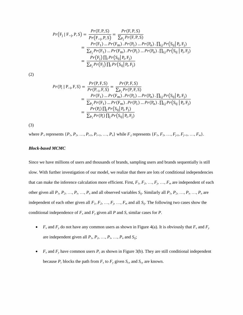
where P-i represents {P1, P2, …, Pi-1, Pi+1, …, Pn} while F-j represents {F1, F2, …, Fj-1, Fj+1, …, Fm}.
Block-based MCMC
Since we have millions of users and thousands of brands, sampling users and brands sequentially is still
slow. With further investigation of our model, we realize that there are lots of conditional independencies
that can make the inference calculation more efficient. First, F1, F2, …, Fj, …, Fm are independent of each
other given all P1, P2, …, Pi, …, Pn and all observed variables Sij. Similarly all P1, P2, …, Pi, …, Pn are
independent of each other given all F1, F2, …, Fj, …, Fm and all Sij. The following two cases show the
conditional independence of Fx and Fy given all P and S, similar cases for P.
Fx and Fy do not have any common users as shown in Figure 4(a). It is obviously that Fx and Fy
are independent given all P1, P2, …, Pi, …, Pn and Sij;
Fx and Fy have common users Pc as shown in Figure 3(b). They are still conditional independent
because Pc blocks the path from Fx to Fy given Scx and Scy are known.
Figure 4. Illustration of conditional independence*
* Two cases for the conditional independence of Fx and Fy, given all P and S. Shaded variables means are known.
These conditional independencies give us opportunities to sample brands and users in parallel. Thus, we
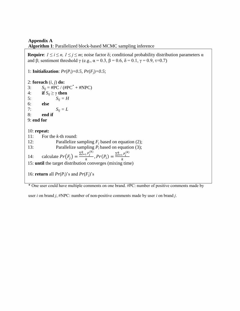
implement a block-based MCMC method that processes users and brands as two separate blocks. We
alternately sample all Pi’s and Fj’s in each sampling round. The detailed algorithm is depicted in
Algorithm 1 in Appendix A. Performance comparison between our parallelized block-based MCMC and
sequential MCMC is presented in Appendix B.
RESULTS
We apply our model to all seven years of data (all comments and likes posted by all users across all
brands) to obtain user positivity scores for each of the 169.57 million users and brand favorability scores
for each of the 3,355 brands in our data. These user positivity and brand favorability scores refer to the
posterior estimate of each user’s probability of being high positivity and each brand’s probability of being
high favorability, respectively. We assume that user positivity is a user trait and therefore is relatively
static. However, we acknowledge that brand favorability can change over time and therefore re-calculate
brand favorability probabilities (all Fj’s) based only on the sentiment of user engagements (Sij’s) from just
one year, 20159. It is important to note that this is a very large dataset that poses some serious challenges
9 We also estimated the model using only data from 2015 to estimate both user positivity and brand favorability.
The results were very similar, with brand favorability scores correlated 0.91 across the two methods. Furthermore, no significant differences were observed in any of the subsequent analyses.
for estimation. Beyond just the issue of computing power (we estimated the model on a machine with 256
GB memory and 24 cores), we also made some simplifying assumptions regarding the conditional
probability distribution presented in Table 2.
Our model contains four parameters as shown in Table 2 and one threshold parameter . Given the size of
the data, it is infeasible to use traditional Bayesian methods to estimates these parameters. Instead, we
estimated the resulting brand favorability and user positivity measures using each of 2304 possible
parameter combinations, assuming that each parameter potentially has 9 discrete values with a range [0.1,
0.9] subject to the following simplifying constraints: (1) α < β; (2) <0.5, >0.5, >0.510
. For each
parameter setting, we calculated the log-likelihood of the model. These log-likelihoods ranged from -
9.12x10⁸ to -4.08x10
8. The parameter combination with the maximum log-likelihood (α = 0.3, β = 0.6, δ
= 0.1, γ = 0.9, =0.7, LL = -4.08x10⁸) was chosen to generate the results we present next. Later in this
section, we discuss the sensitivity of our results to the various parameter settings.
Figure 5 provides a histogram of user positivity scores across all users while Figure 6 provides a
histogram of brand favorability scores across all brands in our data. The distribution of user positivity
scores presented in Figure 5 indicates significant differentiation across users in terms of their innate
tendencies to be positive. This provides empirical evidence that scale usage heterogeneity exists and has
the potential to bias sentiment metrics. Figure 6, not surprisingly, also shows dispersion in brand
favorability scores.
Figure 6 shows a clear positive skew in brand favorability scores. This positive skew is not surprising
given that brands can only persist if consumers have a positive opinion of it. This is not to say that all
10
If estimation results indicate that these constraints are binding, they can be relaxed later.
brands are favorably perceived. In fact, in our data, 17.9% of the brands are extremely favorable (i.e.,
brand favorability > 0.9) and less than 1% have favorability scores below 0.5.
Figure 5. Distribution of user positivity scores
Figure 6. Distribution of 2015 brand favorability scores
0
5,000,000
10,000,000
15,000,000
20,000,000
25,000,000
30,000,000
35,000,000
40,000,000
45,000,000
0-0.1 0.1-0.2 0.2-0.3 0.3-0.4 0.4-0.5 0.5-0.6 0.6-0.7 0.7-0.8 0.8-0.9 0.9-1.0
Nu
mb
er
of
Use
rs
User Positivity
0
200
400
600
800
1000
1200
1400
0-0.1 0.1-0.2 0.2-0.3 0.3-0.4 0.4-0.5 0.5-0.6 0.6-0.7 0.7-0.8 0.8-0.9 0.9-1.0
Nm
be
r o
f B
ran
ds
Brand Favorability
Table 3. Summary of brand favorability scores across parameter settings
Top 20 Favorability score* Mean Std. Dev. Minimum Maximum
Google 0.826 0.754 0.004 0.746 0.826
Microsoft 0.780 0.761 0.003 0.753 0.780
IBM 0.850 0.848 0.003 0.841 0.854
Visa 0.762 0.759 0.003 0.750 0.769
ATT 0.634 0.606 0.006 0.594 0.634
Verizon 0.739 0.743 0.005 0.731 0.754
Coca-Cola 0.782 0.778 0.004 0.767 0.789
McDonald's 0.702 0.677 0.002 0.672 0.702
Facebook 0.877 0.817 0.003 0.809 0.877
Alibaba 0.783 0.749 0.002 0.744 0.783
Amazon.com 0.799 0.776 0.003 0.768 0.799
Wells Fargo 0.841 0.880 0.004 0.841 0.888
GE 0.818 0.839 0.004 0.818 0.848
UPS 0.863 0.862 0.003 0.854 0.870
Disney 0.994 0.970 0.003 0.963 0.994
MasterCard 0.814 0.740 0.003 0.732 0.814
Vodafone UK 0.657 0.656 0.005 0.644 0.669
SAP 0.796 0.778 0.004 0.766 0.796
American Express 0.775 0.781 0.003 0.772 0.789
Wal-Mart 0.769 0.751 0.003 0.741 0.769
Bottom 20 Favorability score* Mean Std. Dev. Minimum Maximum
Ford 0.681 0.655 0.003 0.646 0.681
BP 0.720 0.757 0.003 0.720 0.765
Telstra 0.703 0.685 0.004 0.674 0.703
KFC 0.692 0.697 0.002 0.689 0.704
Westpac 0.655 0.645 0.002 0.640 0.655
LinkedIn 0.726 0.741 0.002 0.726 0.749
Santander Bank 0.691 0.690 0.002 0.684 0.696
Woolworths 0.723 0.747 0.003 0.723 0.754
PayPal 0.640 0.667 0.002 0.640 0.674
Chase 0.693 0.708 0.006 0.689 0.727
ALDI USA 0.790 0.775 0.002 0.769 0.790
ING 0.810 0.797 0.002 0.790 0.810
Twitter 0.711 0.716 0.005 0.704 0.729
Nissan 0.788 0.797 0.006 0.783 0.810
Red Bull 0.701 0.681 0.003 0.673 0.701
Bank of America 0.739 0.703 0.003 0.695 0.739
NTT DOCOMO 0.600 0.608 0.003 0.600 0.616
Costco 0.661 0.641 0.003 0.630 0.661
SoftBank 0.633 0.632 0.004 0.620 0.643
Scotiabank 0.687 0.696 0.004 0.687 0.705
* Based on parameter settings that yielded maximum likelihood (α = 0.3, β = 0.6, δ = 0.1, γ = 0.9, =0.7)
To reiterate, the brand favorability and user positivity scores presented above are associated with the
parameter combination: α = 0.3, β = 0.6, δ = 0.1, γ = 0.9, =0.7. This is the parameter setting that yielded
the largest log-likelihood. To test how sensitive our results are to the parameter settings, we compute
brand favorability scores associated with each of the 2304 parameter combinations and examine the
variance in estimates across different parameter settings. Table 3 summarizes metrics describing how
brand favorability varies across parameter settings for the 20 top brands and 20 bottom brands in
Millward Brown’s BrandZ Top 100 rankings. The results show that there is very little variation in brand
favorability. In other words, brand favorability scores resulting from our model are not very sensitive to
the parameter combination selected to initiate the model. This gives us confidence in our methodology
and in the robustness of the brand favorability scores that result.
Model Fit
To assess model fit, we test how well it can accurately predict the sentiment of unseen comments when
brand favorability and user positivity are given. We first divide our data into a training set and a testing
set in the following way. For each brand, we randomly select 70% of the comments for the training set.
The remaining 30% are used for the testing set. We then estimate our model on the training set to obtain
brand favorability for all brands and user positivity for all individuals. We use these brand favorability
and user positivity estimates to predict the binary sentiment (positive vs. non-positive) of comments in the
testing set, using the same threshold () as in the model estimation.
Table 4 presents the results of our model fit testing. Our model has a high accuracy rate of 88.1%. That is,
the model correctly classifies 88.1% of the comments as positive or non-positive in the testing set.
Turning to our measure of precision, of the comments that we predicted to be positive, 86.9% were
actually observed to be positive. In terms of recall, 89.1% of the observed positive comments were also
predicted to be positive by our model. Overall, these measures indicate that our model of brand
favorability and user positivity fits the observed data well.
Table 4: Model fit
Accuracy1 0.881
Precision2 0.869
Recall3 0.891
RMSE4 0.203
1 Accuracy is defined as the proportion of comments in the testing set that were correctly classified as positive
versus non-positive using model predictions. 2 Precision is the proportion of comments predicted to be positive which were actually observed to be positive.
3 Recall is the proportion of positive comments that were correctly identified by the model.
4 Root mean squared error.
Validation of Method
To validate our brand favorability scores, we compare our social-media based measure of brand
favorability against Millward Brown’s BrandZ ranking of the top 100 most valuable global brands in
2015. The brand favorability and the user positivity scores obtained from our system are based on all user
user-brand interactions across seven years (2009-2016).
On average, the top 20 brands according to BrandZ had a mean favorability score of 0.793 while the
bottom 20 brands had a favorability score of 0.702. This difference is significant with p-value < 0.001,
providing initial confidence in our ability to predict BrandZ outcomes with our proposed brand
favorability score. We further examine the relationship between our method and Millward Brown’s by
regressing both the BrandZ rank and estimated value against our social media based brand favorability
score (see Table 5). For comparison purposes, we also consider the effectiveness of a model-free social-
media based measure, average sentiment, in predicting BrandZ rank and value (also presented in Table 5).
The results show that our proposed brand favorability measure significantly predicts Millward Brown’s
BrandZ rank and value (which are based on both financial performance metrics and brand tracking
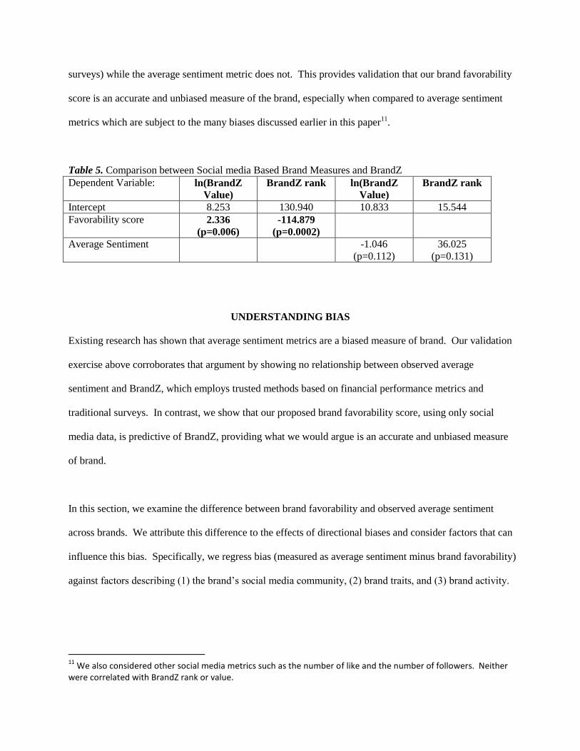
surveys) while the average sentiment metric does not. This provides validation that our brand favorability
score is an accurate and unbiased measure of the brand, especially when compared to average sentiment
metrics which are subject to the many biases discussed earlier in this paper11
.
Table 5. Comparison between Social media Based Brand Measures and BrandZ
Dependent Variable: ln(BrandZ
Value)
BrandZ rank ln(BrandZ
Value)
BrandZ rank
Intercept 8.253 130.940 10.833 15.544
Favorability score 2.336
(p=0.006)
-114.879
(p=0.0002)
Average Sentiment -1.046
(p=0.112)
36.025
(p=0.131)
UNDERSTANDING BIAS
Existing research has shown that average sentiment metrics are a biased measure of brand. Our validation
exercise above corroborates that argument by showing no relationship between observed average
sentiment and BrandZ, which employs trusted methods based on financial performance metrics and
traditional surveys. In contrast, we show that our proposed brand favorability score, using only social
media data, is predictive of BrandZ, providing what we would argue is an accurate and unbiased measure
of brand.
In this section, we examine the difference between brand favorability and observed average sentiment
across brands. We attribute this difference to the effects of directional biases and consider factors that can
influence this bias. Specifically, we regress bias (measured as average sentiment minus brand favorability)
against factors describing (1) the brand’s social media community, (2) brand traits, and (3) brand activity.
11
We also considered other social media metrics such as the number of like and the number of followers. Neither were correlated with BrandZ rank or value.
We characterize a brand’s social media community by considering the variance of sentiment expressed on
the page, the number of followers, the number of comments and the number of likes. We consider
multiple measures for number of followers: (1) number of all followers who have liked the page, (2) the
number of users who have either commented on the brand page or have liked a brand post on the page, (3)
the number of users who have commented on the page, and (4) the number of users who have liked a
brand post on the page. While the first measures the size of the brand’s social media following, the latter
three capture the size of the engaged user base.
We also consider brand traits such as the firm’s industry sector (according to Yahoo!Finance), the size of
the firm, which we represent with number of employees, and overall popularity of the brand, which we
represent with Google Trends data. Finally, we consider brand activity. Specifically, we measure the
number of posts a brand contributes to its own brand page to represent their social media marketing
activity. We also include the number of Yahoo!News mentions to provide a measure of earned media.
A few of the factors described above (i.e., industry sector and number of employees) are available only
for publically traded firms. Thus, as an initial analysis, we examine only the 84 brands in the BrandZ Top
100. Later, we will expand the analysis to include all brands in our data but exclude these factors as
independent variables.
Figure 7 illustrates the distribution in bias across brands, with bias defined as the difference between
average sentiment and brand favorability. The average bias is -0.0245, ranging from a negative bias of -
0.318 to a positive bias 0.314. To explore how this bias varies according to the brand community, brand
trait, and brand activity metrics described above, we segment brand pages into four categories: extreme
negative bias (bias < -0.1), moderate negative bias (-0.1 < bias < 0), moderate positive bias (0 < bias < 0.1)
and extreme positive bias (bias > 0.1). Descriptive metrics for each bias category are presented in Table 6.
Figure 7. Bias across brands (BrandZ Top 100)
Table 6 shows that the brands that experience extreme positive bias on their brand pages tend to have
smaller brand communities with lower variance in sentiment being expressed on the page. Variation in
the number of employees, brand posts and news mentions across bias categories is less systematic. The
summary metrics also show that the Google Trends metric increases with bias, suggesting that bias may
be related to the overall popularity of the brand. However, the results presented in Table 6 only present a
descriptive summary and should not be used to imply attribution.
0
2
4
6
8
10
12
14
16
18
20
[-.3
5,-
.3]
[-.3
,-.2
5]
[-.2
5,-
.2]
[-.2
,-.1
5]
[-.1
5,-
.1]
[-.1
,-.0
5]
[-.0
5,0
]
[0,.
05
]
[.0
5,.
1]
[.1
,.1
5]
[.1
5,.
2]
[.2
,.2
5]
[.2
5,.
3]
[.3
,.3
5]
Nu
mb
er
of
Bra
nd
s
Bias
Table 6. Descriptive metrics by bias category
Extreme Negative
Moderate Negative
Moderate Positive
Extreme Positive
Brand Community
Variance in Sentiment 0.24 0.21 0.22 0.20
# of Followers 7,714,370 10,060,314 2,568,759 2,714,114
# of Engaged Users 1,405,737 1,919,774 742,693 503,643
# of Users Commenting 141,431 191,350 71,004 42,830
# of Users Liking 1,279,624 1,729,734 676,109 460,896
# of Comments 38,792 58,237 25,417 26,000
# of Likes 1,289,345 1,973,437 590,429 449,810
Brand Traits
Number of Employees 112,546 290,004 167,376 121,330
Google Trends 77.17 78.38 78.74 81.06
Brand Activity
# of Brand Posts 258 379 361 374
# of News Mentions 815 1,545 578 2,570
Table 7 presents the results of regression models that more formally examine the effects of each brand
metric on bias for the 84 brands in the BrandZ Top 100. Each column represents a different model
specification, where the only difference across models is how the size of the brand community is defined.
In the first model (MDL1) where the size of the brand community is measured as the total number of
global followers, only brand community measures (i.e., variance and sentiment and total number of global
followers) affects bias. Surprisingly, brand traits (i.e., industry sector, number of employees and Google
Trends) and brand activity (i.e., brand posts and news mentions) have no significant effect. In other words,
the bias can be solely attributed to brand community characteristics and is not a function of the size of the
firm, overall popularity of the brand or any brand activity on the brand page or in earned media12
.
12
Non-linear effects for all variables were also tested and had no significant effects on bias.
Table 7. Bias Model for BrandZ Top 100
MDL1 MDL2 MDL3 MDL4 MDL5
Intercept 0.1347 (0.1681)
0.0885 (0.3561)
0.0956 (0.3192)
0.0876 (0.3615)
0.0742 (0.4388)
Brand Community
Variance in Sentiment -0.7431 (0.0043)
-0.6335 (0.0128)
-0.6243 (0.0136)
-0.6320 (0.0130)
-0.6965 (0.0071)
# of Followers (000,000s) -0.0029 (0.0216)
# of Engaged User (000,000s)
-0.0119 (0.0795)
# of Users Commenting (000,000s)
-0.1165 (0.0616)
# of Users Liking (000,000s)
0.0128 (0.0849)
# of Comments (000,000s)
-0.1717 (0.3393)
# of Likes (000,000s)
0.0074 (0.0848)
Brand Traits
Sector[Basic Materials] 0.0545 (0.3593)
0.0526 (0.3848)
0.0540 (0.3705)
0.0527 (0.3839)
0.0542 (0.3678)
Sector[Consumer Goods] -0.0036 (0.9023)
-0.0062 (0.8349)
-0.0123 (0.6782)
-0.0057 (0.8485)
0.0021 (0.9455)
Sector[Financial] 0.0409 (0.1459)
0.0406 (0.1559)
0.0420 (0.1405)
0.0406 (0.1565)
0.0426 (0.1342)
Sector[Industrial Goods] -0.0741 (0.3604)
-0.0704 (0.3918)
-0.0671 (0.4127)
-0.0705 (0.3915)
-0.0803 (0.3292)
Sector[Services] -0.0320 (0.2991)
-0.0304 (0.3399)
-0.0302 (0.3403)
-0.0309 (0.3310)
-0.0300 (0.3428)
# Employees (000,000s) 0.0388
(0.2462) 0.0325
(0.3357) 0.0358
(0.2888) 0.0319
(0.3442) 0.0262
(0.4374) GoogleTrends -0.0270
(0.7786) 0.0007
(0.9946) -0.0192 (0.8433)
0.0007 (0.9939)
0.0224 (0.8214)
Brand Activity
# of Brand Posts (000s) 0.0691 (0.0783)
0.0752 (0.0624)
0.0864 (0.0379)
0.0737 (0.0670)
0.1093 (0.0180)
# of News Mentions (0,000s) 0.0462
(0.3439) 0.0031
(0.5164) 0.0041
(0.4152) 0.0030
(0.5407) 0.0020
(0.6811)
R-Squared 0.2578 0.2336 0.2383 0.2324 0.2508
Adjusted R-Squared 0.1395 0.1114 0.1168 0.1100 0.1185
* p-values are presented in parentheses
The brand community effects are interesting as the results complement previous research findings. First,
we see that variance in sentiment has a negative effect on bias. That is, communities with a wide variety
of opinion tend to be more negatively biased. This is consistent with Moe and Schweidel (2012) who
showed how a diversity of opinions can drive users to offer increasingly negative opinions, regardless of
what their true underlying opinion may be. However, the corollary is also interesting. That is, the less
variability in opinions that exists on the brand page, the more positive the bias. This suggests that
communities in which members share the same opinions may reinforce each other’s positive affinity for
the brand in an “echo chamber” type effect.
Contributing to the sentiment variance effect is the fact that the number of followers has a negative effect
on bias. In other words, the smaller your brand community, the more positive the bias, and the larger
your community, the more negative the bias. This again suggests that a small, uniform community of
followers may reinforce each others’ positive affinity for the brand and potentially create “echo chamber”
effects where a positive bias emerges from the community. As an illustration, consider four brands:
PayPal, Oracle, Nike and Disney (see Table 8). The two smaller social media communities (i.e., PayPal
and Oracle) tend to receive more positive posts than their brand favorability would suggest, whereas the
two larger communities (i.e., Nike and Disney) receive more negative posts than likely is deserved. This
is despite the fact that Disney and Nike were both ranked higher than PayPal and Oracle by Millward
Brown’s BrandZ methodology. In fact, according to the average sentiment metric, Oracle should be the
highest ranking brand among the four described in Table 8. However, Millward Brown actually ranked
Disney the highest among the four, a position with which our proposed favorability score concurs. In
other words, the opinions posted to Disney’s brand page does not reflect the positive value of the brand.
We would argue that this is due to the negative bias induced by their large number social media
community. In contrast, Oracle, which has a smaller social media community, is subject to a positive bias,
and average sentiment metrics overstate the favorability of their brand.
Table 8. Illustration of Community Size Effects on Bias
Brand BrandZ Rank Avg Sent Favorability Bias # Followers
PayPal 88 0.8009 0.6401 0.1608 395,751
Oracle 44 0.9189 0.7977 0.1212 475,935
Nike 28 0.7372 0.8524 -0.1152 20,604,708
Disney 19 0.8752 0.9941 -0.1189 34,726,558
The remaining columns in Table 7 (MDL2 – MDL 5) provide the same analysis using different metrics to
represent the size of the brand community. Rather than characterizing the overall size of the brand
community, these alternative measures better capture the size of the engaged community (i.e., number of
engaged followers who have either commented on the page or have liked a brand post (MDL2), number
of followers commenting (MDL3), or number of followers liking (MDL4)) or the level of engagement
activity on the brand page (i.e., the number of comments and the number of likes, MDL5). In each of
these alternative model specifications, the effect of community size is only marginally significant but
directional consistent with the results of MDL1. This suggests that bias is not necessarily driven by the
level of engagement on the page. Instead, the overall size of the community, regardless of the volume of
engagement, and the variance in sentiment when users do engage are what affect bias.
We next extend our analysis to the larger dataset of 3,355 brand pages. Interestingly, we find notable
difference between brand pages belonging to commercial brands and pages belonging to other types of
brands such as celebrities, sports teams, non-profit organizations and interest groups, etc. Table 9
presents results when we consider (1) all brand pages, (2) only commercial brand pages or (3) other brand
pages. For the 1,139 commercial brands in our data set, the results do not differ from our analysis of the
BrandZ Top 100 brands in that small communities where members share similar opinions are more likely
to be positively biased. However, for other types of brand pages, there is no significant effect of the
number of followers, though the negative effect of sentiment variance remains. One explanation is that
people who follow celebrities, sports teams and other special interests are “super fans” and are unlikely to
provide negative feedback. Additionally, there is no redress for posting negative comments on a celebrity
page as there may be when a negative comment is posted to a commercial brand page (Ma, Sun and
Kekre 2015). This is an interesting difference which we will leave for future research.
Table 9. Bias Model for All Brands
All pages
(n=3,343)
Commercial
brand pages
(n=1,143)
Other pages
(n=2,200)
Intercept 0.0364 (<0.0001)
0.0620 (<0.0001)
0.0239 (0.0047)
Brand Community Variance in Sentiment -0.1767
(<0.0001) -0.3370
(<0.0001) -0.1213 (0.0005)
# of Followers (0,000,000) 0.0002
(0.9244) -0.0100 (0.0196)
0.0015 (0.4025)
Brand Traits GoogleTrends -0.0023
(0.6221) 0.0035
(0.6866) 0.0038
(0.5240)
Brand Activity # of Brand Posts (000s)
0.0126
(0.0438) 0.0215
(0.3509) 0.0090
(0.1623) # of News Mentions (0,000)
0.0019
(0.9304) 0.0334
(0.1636) 0.2533
(0.6767) NOTE: The Facebook Insight API returned no follower counts for 12 brand pages. These pages were removed from
the dataset of 3,355 for analysis.
* p-values are presented in parentheses.
Implications for Brand Communities
Our research has shown not only that directional bias exists on social media brand pages but smaller
communities with limited variance in opinions are positively biased. This suggests that these communities
may be subject to echo chamber effects where the opinions of a few reinforce the positive opinions
expressed by others (while suppressing negative opinions) and lead to a positivity bias. This dynamic
may limit the value of the community as a source for insights. Managers who turn to social media
opinions to guide their marketing activities, solicit input for product design, or manage their customer
relationships need to be aware of this bias when interpreting and leveraging observed social media data.
However, one could argue that the loss of integrity in insights is acceptable if the positive word-of-mouth
provides benefits in the form of sales, customer relationships and financial performance. Unfortunately,
our research also shows that the biased sentiment measures are not related to BrandZ measures, which
should reflect these benefits. In other words, these biased communities are compromised in their ability
to provide insights without offering the traditional benefits associated with positive word-of-mouth.
From a brand manager perspective, it may be wiser to build a larger and more diverse brand community
online to minimize the bias expressed on the brand page.
CONCLUSION
In this paper, we have argued that directional bias exists on social media brand pages and have proposed a
method that provides a brand favorability measure that accounts for individual differences in providing
positive (or negative) opinions on social media. This research contributes to a growing stream of social
media research that examines bias in online opinion. It also contributes to a growing body of
methodological research focused on providing methods to use social media for accurate and unbiased
insights.
We also examined bias across different brand pages and identified factors that are associated with bias.
Specifically, we show that small social media communities where members share similar opinions are
subject to a positivity bias. This has implications for brand communities and how marketers can leverage
those communities.
While we identified a number of factors that can impact bias, such as variance in sentiment, number of
followers, and number of news mentions, there are still other unknown factors worth investigating. For
example, we show differences between commercial brands and other types of brands, such as celebrities,
sports teams, and non-profit organizations and interest groups. However, we leave further investigation
of these differences to future research. Further, we have focus on examining bias from a brand’s
perspective. Future research on bias at the individual user level would also be highly valuable. That is,
what characteristics of users drive directional bias on social media.
Overall, social media has the potential to be a valuable source of insights for marketers. However, the
data are biased, and as a field, marketing researchers have only just begun exploring ways to debias and
leverage the data for insights. We hope this paper contributes to that effort and provides some answers as
well as some question for marketing managers and researchers.
REFERENCES
Baumgartner, Hans and Jan-Benedict Steenkamp (2001), “Response styles in marketing research: A
cross-national investigation,” Journal of Marketing Research, 38(2), 143-156.
Baxter, R. J. (1982), “Critical antiferromagnetic square-lattice Potts model,” In Proceedings of the Royal
Society of London A: Mathematical, Physical and Engineering Sciences, The Royal Society,
383(1784), 43-54.
Bayus, Barry L. (2013), “Crowdsourcing new product ideas over time: An analysis of the Dell IdeaStorm
community,” Management science, 59(1), 226-244.
Kharif, Olga (2012), “’Lifejacking’: Spammers Hit Social Media,” Bloomberg, May 24,
https://www.bloomberg.com/news/articles/2012-05-24/likejacking-spammers-hit-social-media
(downloaded January 10, 2017).
Bollen, Johan, Huina Mao, and Xiao-Jun Zeng (2011), “Twitter mood predicts the stock market,” Journal
of Computational Science, 2(1), 1-8.
Chevalier, Judith A. and Dina Mayzlin (2006), “The effect of word of mouth on sales: Online book
reviews,” Journal of Marketing Research, 43(3), 345-354.
Choi, Yejin and Claire Cardie (2008), “Learning with compositional semantics as structural inference for
subsentential sentiment analysis,” The Conference on Empirical Methods in Natural Language
Processing (EMNLP’08), ACL, Stroudsburg, PA 793-801.
Kelly, Heather (2012), “83 Million Facebook accounts are fakes and dupes,” CNN, August 3,
http://www.cnn.com/2012/08/02/tech/social-media/facebook-fake-accounts/ (downloaded January 10,
2017).
Fiebig, Denzil G., Michael P. Keane, Jordan Louviere, and Nada Wasi (2009), “The generalized
multinomial logit model: accounting for scale and coefficient heterogeneity,” Marketing Science,
29(3), 393-421.
Godes, David and Jose C. Silva (2011), “Sequential and temporal dynamics of online opinion,”
Marketing Science, 31(3):448-473.
Lee, Thomas Y., and Eric T. Bradlow (2011), "Automated marketing research using online customer
reviews," Journal of Marketing Research, 48 (5), 881-894.
Lehmann, Donald R., Kevin Lane Keller, and John U. Farley (2008), “The structure of survey-based
brand metrics,” Journal of International Marketing, 16(4), 29-56.
Li, Xinxin and Lorin M. Hitt (2008), “Self-selection and information role of online product reviews,”
Information System Research, 19(4), 456-474.
Ma, Liye, Baohong Sun, and Sunder Kekre (2015), “The Squeaky Wheel Gets the Grease—An empirical
analysis of customer voice and firm intervention on Twitter,” Marketing Science, 34(5), 627-645.
Moe, Wendy W. and David A. Schweidel (2012), “Online product opinions: Incidence, evaluation, and
evolution,” Marketing Science, 31(3), 372-386.
Mukherjee, Arjun, Bing Liu, and Natalie Glance (2012), “Spotting fake reviewer groups in consumer
reviews,” The 21st international conference on World Wide Web (WWW’12), ACM, New York, NY,
USA, 191-200.
Mukherjee, Arjun, Abhinav Kumar, Bing Liu, Junhui Wang, Meichun Hsu, Malu Castellanos, and
Riddhiman Ghosh (2013), “Spotting opinion spammers using behavioral footprints,” The SIGKDD
International Conference on Knowledge Discovery and Data Mining (KDD’13), Chicago, USA.
Netzer, Oded, Ronen Feldman, Jacob Goldenberg, and Moshe Fresko, "Mine your own business: Market-
structure surveillance through text mining," Marketing Science 31, no. 3 (2012): 521-543.
Pang, Bo and Lillian Lee (2008), “Opinion mining and sentiment analysis,” Foundations and Trends in
Information Retrieval, 2(1-2), 1-135.
Park, C.S. and Srinivasan, V. (1994), “A survey-based method for measuring and understanding brand
equity and its extendibility,” Journal of Marketing Research, pp.271-288.
Paulhus, Delroy L. (1991), "Measurement and control of response bias."
Rossi, Peter E., Zvi Gilula, and Greg M. Allenby (2001), “Overcoming scale usage heterogeneity: A
Bayesian hierarchical approach,” Journal of the American Statistical Association, 96(453), 20-31.
Schau, H.J., Muñiz Jr, A.M. and Arnould, E.J. (2009), “How brand community practices create value,”
Journal of Marketing, 73(5), pp.30-51.
Schlosser, Ann E. (2005), “Posting versus lurking: Communicating in a multiple audience context,”
Journal of Consumer Research, 32(2), 260-265.
Schweidel, David A. and Wendy W. Moe (2014), “Listening in on social media: a joint model of
sentiment and venue format choice,” Journal of Marketing Research, 51(4), 387-402.
Tirunillai, Seshadri, and Gerard J. Tellis (2012), "Does chatter really matter? Dynamics of user-generated
content and stock performance," Marketing Science, 31(2), 198-215.
Trusov, Michael, Randolph E. Bucklin, and Koen Pauwels (2009), "Effects of word-of-mouth versus
traditional marketing: findings from an internet social networking site," Journal of Marketing, 73 (5),
90-102.
Xie, Yusheng, ZhengZhang Chen, Kunpeng Zhang, Yu Cheng, Daniel Honbo, Ankit Agrawal, Alok
Choudhary (2013), “MuSES: Multilingual Sentiment Elicitation System for Social Media,” IEEE
Intelligent Systems.
Zhang, Kunpeng, Yu Cheng, Yusheng Xie, Daniel Honbo, Wei-keng Liao, and Alok Choudhary (2011),
“SES: Sentiment Elicitation System for Social Media Data,” The 11th ICDM Workshops, Vancouver,
Canada.
Appendix A
Algorithm 1: Parallelized block-based MCMC sampling inference
* One user could have multiple comments on one brand. #PC: number of positive comments made by
user i on brand j, #NPC: number of non-positive comments made by user i on brand j.
Require: 1 ≤ i ≤ n, 1 ≤ j ≤ m; noise factor δ; conditional probability distribution parameters α
and β; sentiment threshold γ (e.g., α = 0.3, β = 0.6, δ = 0.1, γ = 0.9, =0.7)
1: Initialization: Pr(Pi)=0.5, Pr(Fj)=0.5;
2: foreach (i, j) do:
3: Sij = #PC / (#PC* + #NPC)
4: if Sij ≥ γ then
5: Sij = H
6: else
7: Sij = L
8: end if
9: end for
10: repeat:
11: For the k-th round:
12: Parallelize sampling Fj based on equation (2);
13: Parallelize sampling Pi based on equation (3);
14: calculate 𝑃𝑟(𝐹𝑗) =∑ 𝐹𝑗
(𝑘)𝑘𝑡=1
𝑘, 𝑃𝑟(𝑃𝑖) =
∑ 𝑃𝑖(𝑘)𝑘
𝑡=1
𝑘
15: until the target distribution converges (mixing time)
16: return all Pr(Pi)’s and Pr(Fj)’s
Appendix B
Performance evaluation
Two common important aspects related to MCMC-based inference algorithm are: 1) the
convergence speed, 2) the time complexity of sampling. To investigate the first aspect, we
randomly pick 5 brands from different categories and plot their favorability scores as the
sampling proceeds. Fig. 7 clearly shows that they converge after we collect about approximately
150~200 samples (we also call this mixing time).
Figure 7. The favorability score convergence of the block-based MCMC algorithm for five
different brands
To address the second aspect, we parallelize block-based MCMC due to conditional
independency and compare to the sequential version in terms of time taken. Speedup is a very
common metric used in the field of parallelization. In this experiment, we use 8 processors in
parallel. Fig. 8 shows that we achieve near-linear speedup (close to 7). It is the speedup with
respect to the cumulative time until 50th
, 100th
, …, 500th
sampling round. We believe that the
reason for slightly uneven speedup at some sampling rounds is that MCMC is a stochastically
approximate sampling technique based on the target distribution as shown in equation (2) and
0
0.2
0.4
0.6
0.8
1
1 51 101 151 201 251 301 351 401 451
American Express BMW United Airline Gucci Microsoft
equation (3). Experiments were run on a machine with 256 GB memory and 24 cores. Sp=T1/Tp,
where p is the number of processors (p = 8 here); T1 is the execution time of sequential algorithm;
Tp is the execution time of parallel algorithm with p processors.
Figure 8. Speedup of the parallelized block-based MCMC algorithm over the sequential
algorithm on 8 computing cores
6.8
6.85
6.9
6.95
7
7.05
50 100 150 200 250 300 350 400 450 500
Sp
eed
up
Sampling round