Biasing a ring-oscillator based true random number ... · Biasing a ring-oscillator based true...

Biasing a ring-oscillator based true randomnumber generator with an electro-magnetic fault

injection using harmonic waves.

Jeroen Senden

Master Thesis

Committee:dr. M.H. Everts

dr. A. Peterdr. ir. F. de Beer

Institution:University of Twente

Chair:Distributed and Embedded Security

14-01-2015

2

Abstract

This thesis shows the effect of an electromagnetic fault injection ontrue random number generators based on ring oscillators. It testsseveral designs, including ring oscillators of equal length and unequallength. We found that the created designs with ring oscillators ofunequal length are more prone to fault injection. This research alsoshows that injecting the frequency of the operating frequency of thering oscillators results in high mutual information. Fault injectionusing an electro-magnetic harmonic signal has a global effect, butalso has local effects. An injection close to a wire connected to thering oscillators seems like a good injection area.

3

4

Contents

1 Introduction 9

1.1 Scenario . . . . . . . . . . . . . . . . . . . . . . . . . . . . . . . . 9

1.2 Random number generation . . . . . . . . . . . . . . . . . . . . . 12

1.3 Attacks . . . . . . . . . . . . . . . . . . . . . . . . . . . . . . . . 13

1.3.1 Active vs. Passive . . . . . . . . . . . . . . . . . . . . . . 13

1.3.2 Invasive, semi-invasive, non-invasive . . . . . . . . . . . . 13

1.3.3 Fault injection . . . . . . . . . . . . . . . . . . . . . . . . 14

1.3.4 This research . . . . . . . . . . . . . . . . . . . . . . . . . 14

1.4 True random number generators . . . . . . . . . . . . . . . . . . 14

1.5 Noise . . . . . . . . . . . . . . . . . . . . . . . . . . . . . . . . . . 15

1.5.1 Shot noise . . . . . . . . . . . . . . . . . . . . . . . . . . . 15

1.5.2 Thermal noise . . . . . . . . . . . . . . . . . . . . . . . . 15

1.6 TRNG using ring oscillators . . . . . . . . . . . . . . . . . . . . . 15

1.6.1 Theoretical overview . . . . . . . . . . . . . . . . . . . . . 16

1.6.2 Equal ring length . . . . . . . . . . . . . . . . . . . . . . . 18

1.6.3 Different ring length . . . . . . . . . . . . . . . . . . . . . 18

1.7 Research questions . . . . . . . . . . . . . . . . . . . . . . . . . . 19

2 Related work 21

2.1 Cartography . . . . . . . . . . . . . . . . . . . . . . . . . . . . . . 21

2.2 Attacks . . . . . . . . . . . . . . . . . . . . . . . . . . . . . . . . 22

2.3 EM fault injection using harmonic emission . . . . . . . . . . . . 22

2.4 EM fault injection using pulses . . . . . . . . . . . . . . . . . . . 24

2.5 EM countermeasures . . . . . . . . . . . . . . . . . . . . . . . . . 24

3 Setup 25

3.1 Overview . . . . . . . . . . . . . . . . . . . . . . . . . . . . . . . 25

3.2 Probes . . . . . . . . . . . . . . . . . . . . . . . . . . . . . . . . . 26

3.3 Targets . . . . . . . . . . . . . . . . . . . . . . . . . . . . . . . . 27

3.4 Verification methods . . . . . . . . . . . . . . . . . . . . . . . . . 27

3.4.1 Finding the optimal injection frequency . . . . . . . . . . 27

3.4.2 Mutual information . . . . . . . . . . . . . . . . . . . . . 29

3.4.3 Random number test suites . . . . . . . . . . . . . . . . . 30

5

6 CONTENTS

4 Initial experiments on a TRNG 31

4.1 Design . . . . . . . . . . . . . . . . . . . . . . . . . . . . . . . . . 31

4.2 Initial experiments . . . . . . . . . . . . . . . . . . . . . . . . . . 32

4.2.1 Injection of 220 MHz . . . . . . . . . . . . . . . . . . . . . 32

4.2.2 Injection of 300 MHz . . . . . . . . . . . . . . . . . . . . . 33

4.2.3 Mutual information . . . . . . . . . . . . . . . . . . . . . 34

4.3 Conclusion . . . . . . . . . . . . . . . . . . . . . . . . . . . . . . 35

5 TRNG implemented with 5 ROs 37

5.1 Design . . . . . . . . . . . . . . . . . . . . . . . . . . . . . . . . . 37

5.2 Frequency sweep . . . . . . . . . . . . . . . . . . . . . . . . . . . 38

5.3 Mutual information . . . . . . . . . . . . . . . . . . . . . . . . . . 41

5.4 Power sweep . . . . . . . . . . . . . . . . . . . . . . . . . . . . . . 42

5.5 RNG test suite result . . . . . . . . . . . . . . . . . . . . . . . . . 43

5.6 Conclusion . . . . . . . . . . . . . . . . . . . . . . . . . . . . . . 43

6 Injection on different implementation designs 47

6.1 Initial experiment . . . . . . . . . . . . . . . . . . . . . . . . . . . 47

6.1.1 Frequency sweep & mutual information . . . . . . . . . . 48

6.2 Designs . . . . . . . . . . . . . . . . . . . . . . . . . . . . . . . . 49

6.2.1 Scanning area . . . . . . . . . . . . . . . . . . . . . . . . . 49

6.2.2 The chosen designs . . . . . . . . . . . . . . . . . . . . . . 50

6.2.3 Flow of an experiment . . . . . . . . . . . . . . . . . . . . 51

6.3 General remarks . . . . . . . . . . . . . . . . . . . . . . . . . . . 52

6.4 Horizontal vs vertical placement . . . . . . . . . . . . . . . . . . 54

6.5 With antenna vs without antenna . . . . . . . . . . . . . . . . . . 54

6.6 Inline vs parallel placement . . . . . . . . . . . . . . . . . . . . . 55

6.7 ROs of different length . . . . . . . . . . . . . . . . . . . . . . . . 55

6.8 Conclusion . . . . . . . . . . . . . . . . . . . . . . . . . . . . . . 56

7 Conclusion 59

8 Future work 61

A Additional TRNGs 63

A.1 Quantum optical . . . . . . . . . . . . . . . . . . . . . . . . . . . 63

A.1.1 Photon detection time . . . . . . . . . . . . . . . . . . . . 63

A.1.2 Polarization . . . . . . . . . . . . . . . . . . . . . . . . . . 64

A.1.3 The combination . . . . . . . . . . . . . . . . . . . . . . . 64

A.2 Radioactive decay . . . . . . . . . . . . . . . . . . . . . . . . . . 64

A.3 Chaos-based True Random Number Generator . . . . . . . . . . 65

A.3.1 Analog phenomena . . . . . . . . . . . . . . . . . . . . . . 65

A.3.2 Digital phenomena . . . . . . . . . . . . . . . . . . . . . . 65

CONTENTS 7

B TestTool 67B.1 Introduction . . . . . . . . . . . . . . . . . . . . . . . . . . . . . . 67B.2 Initial experiment . . . . . . . . . . . . . . . . . . . . . . . . . . . 67B.3 Frequency sweeps . . . . . . . . . . . . . . . . . . . . . . . . . . . 68B.4 Visual random numbers . . . . . . . . . . . . . . . . . . . . . . . 68B.5 Temperature . . . . . . . . . . . . . . . . . . . . . . . . . . . . . 70B.6 Conclusion . . . . . . . . . . . . . . . . . . . . . . . . . . . . . . 71

C Frequency sweeps on 2 ROs 73

D Experiments with a short probe 75

E All results of different designs 77

8 CONTENTS

Chapter 1

Introduction

Cryptography has been around for ages and is the main reason why we cancommunicate safely in the digital world (for example in internet banking). Mostcryptographic functions need a random number, which is unpredictable, in orderto work. This random number is used for a lot of cryptographic functions, suchas the creation of a secret key, an initialization vector to start of a cryptographicalgorithm or to prevent replay attacks. Should this random number becomebiased, the whole cryptographic function would become insecure.

There has already been extensive research done that describes an attackon the random number generator (RNG) by using a laser or electromagnetic(EM) waves. Recently, EM fault injection (FI) by harmonic emission (HE) hasbecome a hot topic since it is a new area of research and countermeasures are notimplemented most of the time. This document will be the basis of a research toinvestigate whether ring oscillator (RO)-based true random number generators(TRNG) in high-end targets can be biased by EM FI using harmonic emission.Before going into details, a scenario that explains why random numbers areimportant and an introduction with basic information will follow next.

1.1 Scenario

This section will describe some possible scenarios that could occur when randomnumbers are not random anymore. Figure 1.1 shows a scenario in an authenti-cation setting where a bad random number causes the protocol to be vulnerableto a replay attack. If the random number would not be biased, a replay attackwould not be possible. The protocol is a public/private-key authentication pro-tocol. A user authenticates himself by decrypting a message that only the usercan decrypt by using his private key. In this example Bob authenticates himselfto Alice. Eve can eavesdrop on their communication and wants to authenticateas Bob to Alice, which should not be possible if the protocol is safe. If therandom number was truly random it would prohibit Eve from doing a replayattack.

9

10 CHAPTER 1. INTRODUCTION

Bob will make the initial communication to Alice that he wants to authenti-cate to her. Alice sends Bob a challenge, which is a random value (R) encryptedby the public key of Bob. Bob is the only one who can decrypt this correctlyusing his private key. He gets the R out of the decrypted message, encrypts itwith the public key of Alice and sends it back to Alice. Alice is the only onewho can decrypt Bob’s message by using her private key. If the R sent by Bobis the same as the R send by herself initially, Bob is truly Bob.

The messages that Eve has is the initial communication of Bob to Alice, anencrypted packet containing R and another encrypted package containing R.Eve has no idea what R was in this communication, since both packets wereencrypted and she doesn’t have the necessary decryption keys. Eve starts hercommunication using the initial message sent by Bob. If the same R is created,Eve will receive a packet which is the same as the one Bob received. She thenknows what she needs to send back (although the contents of the packets looklike gibberish to her) and Alice will think that Eve is Bob, since the two randomvalues R are the same. Note that this scenario will also work if R is based on asmall subset of values. Eve only has to eavesdrop on multiple communicationsin order to make the chance large enough that the challenge she receives is inher subset of eavesdropped communication.

Although the previous scenario is just theoretical, bad random number valueshave occurred in practice in the past. The most famous case of a broken RNGis the Mifare Classic, a contactless smart card. Nohl et al. [25] showed thatthey could consistently create the same nonce (number used once), computedwith the same initial value on a Linear Feedback Shift Register (LFSR). Therandomness would come from timing, and it was used for authentication. Ifone knows the nonce, only two messages are necessary to retrieve the secret keyfrom the card with the help of precomputed rainbow tables. In this case notonly the RNG was predictable when you controlled the timing, but also a badinitial seed played a vital part in the success of this attack.

Another example of a bad RNG was the SecureRandom java class on An-droid, which sometimes produced the same random value. This function wasused by several applications, including bitcoin wallets. A bitcoin wallet is awallet that stores your amount of bitcoins, a digital amount of money. A pri-vate key, a certain ‘address’ of the wallet and a random number are used forsigning transactions. Due to the nature of the signature scheme, the privatekey can be discovered if it is used in two transactions with the same randomvalue and same address. The bitcoin wallets used a deterministic RNG. Bitcointransactions are also publicly available, which makes it easier to find vulnerabletransactions. Private keys were thus leaked and malicious transactions wereperformed. Shortly after it got fixed, the same vulnerability was found for theJavaScript version, which again resulted into malicious transactions. This showsthat a bad RNG can cause serious damage.

These are just some of the possible scenarios that have happened. It showsthat RNGs need to be good and are a vital part of a cryptographic system.Bad RNGs could cause a complete cryptographic system to be undermined andrender it useless and can cause serious damage. The next section will provide

1.1. SCENARIO 11

Bob Alice Eve

Hi, I’m Bob

Create R

c=encrypt(R, pbkey Bob)

Ok, proof it. Decrypt c

r’=decrypt(c,prkey Bob)

c’=encrypt(r’, pbkey Alice)

c’

r”=decrypt(c’,prkey Alice)

if r” == R

You are authenticated as Bob

Hi, I’m Bob

Create same R

c=encrypt(R, pbkey Bob)

Ok, proof it. Decrypt c

Previously sent c’ by Bob

r”=decrypt(c’,prkey Alice)

if r” == R

You are authenticated as Bob

Figure 1.1: A authentication protocol using the same random value


some basic information on RNGs, followed by a quick look into some possibleattack methods.

1.2 Random number generation

There are two types of RNGs. First there is the pseudorandom number gener-ator (PRNG). This random number generator does not generate truly randomnumbers, but generates statistical random numbers. A number is statisticallyrandom when it contains no recognizable patterns or regularities and is calcu-lated in a deterministic system. Although these pseudorandom numbers arenot truly random, they are important nonetheless. The generation speed isfast and reproducibility is easy in most cases. The second type of RNG is thetrue random number generator (TRNG). This random number generator doesgenerate truly random numbers and cannot be predicted since they do not relyon previous outcomes. For cryptographic functions a TRNG is preferred over aPRNG. This research focuses on TRNGs and PRNGs are out of scope.

In order to create a random number, one needs an entropy source, a mech-anism to harvest this source and sometimes post-processing:

• The entropy source is the most crucial, since this will determine the ran-domness. The entropy source for a TRNG is a random physical phe-nomenon. A PRNG can collect a number from a true random numbergenerator and run a deterministic function on top of it to create pseu-dorandom numbers. For example, some operating systems use disk in-put/output as an entropy source.

• In order to ‘collect’ entropy, a harvesting mechanism is needed. SomeRNGs employ a XOR as a harvesting mechanism. A XOR take 2 bitwiseinputs. If they are both the same, the output is ‘0’, otherwise the outputis ‘1’. If one of the inputs of the XOR is random, the outcome will alsobe random, making this an excellent harvesting mechanism for a RNG.

• A post-processing phase could be added to strengthen the RNG. The ad-vantage of a post-processor is the fact that it could compensate for envi-ronmental changes or tampering. The disadvantage of a post-processor isthat it will most likely degrade the output speed of random numbers. Acommon post-processor utilizes the von Neumann algorithm. The truthtable for this algorithm is shown in Table 1.1, where x and y are 2 bitwiseinputs to the algorithm.

There are some important features a RNG needs to have to prevent pre-dictability. One of these features is that it needs to produce different randomnumbers each time it is restarted with the same initial value. Later on someTRNGs that need some initial time in order for them to generate random num-bers will be shown (Chapter 1.4).

Although a RNG might produce random numbers at first sight, they mightnot be random nevertheless. There are several suites available in order to verify

1.3. ATTACKS 13

x y out0 0 -0 1 01 0 11 1 -

Table 1.1: Truth table for the Von Neumann post-processing phase

if the generator creates (statistical) random numbers. The DieHarder test-suite[8] and the NIST SP 800-22 test-suite[26] are commonly used, since theytest the most statistical properties that could exist in the random numbers andwould thus not be statistically random. Note that these tests cannot guaranteethat a RNG only produces random numbers. It can only prove that RNGsproduce biased random numbers and are bad RNGs.

1.3 Attacks

To understand the attack that this research proposes, one needs to understandthe different methods of attacking a target. A target is the system under attack,which can be any device that is a security critical system. Attacks can becategorized into groups. The first criteria is based on whether the attack isactive or passive and the second criterion is based on whether the attack isinvasive, semi-invasive or non-invasive. Note that an attack categorized by onecriteria can also be categorized in the second criteria. The two different criteriaare described below.

1.3.1 Active vs. Passive

When an attack is active, this means that the attack entails tampering with thetarget. This tampering can cause unforeseen or abnormal behavior, resultingin for example revealing the secret key. A passive attack is the opposite of anactive attack. A passive attack monitors the target (e.g., power consumptionand execution time) to determine for example a secret key. In an active attack,the target is thus manipulated to do some unforeseen behavior, whereas in apassive attack the target is executing according to its specification.

1.3.2 Invasive, semi-invasive, non-invasive

An invasive attack normally depackages the target and directly accesses partsof the target. Depacking the target makes it possible for the attacker to extractmemory. In a non-invasive attack, the target does not get depackaged. Anexample of this is power analysis (monitoring the power that is consumed) ofthe target. A semi-invasive attack sits in between these two attacks. A semi-invasive attack does depackage the target (e.g., remove the silicon layer from a


smart card), but does not directly interact with the target (shooting a laser atthe depackaged target does not directly interact with the target).

1.3.3 Fault injection

A fault injection (FI), which is the focus of this research, is always an activeattack and can be either invasive (for example the previously mentioned voltageglitching attack) or non-invasive (for example by shooting a laser). A faultinjection can be done in several ways. Lasers could be used to trigger some effect,the supply voltage of the chip could be altered shortly or an electromagneticwave could be send towards the target. The idea of a fault injection is to makethe target execute unwanted behavior, e.g. skip a line of code (software) orcreate a fault in the memory (hardware). When doing a FI, there is the risk ofmaking the target incapable of resuming its normal functionality.

1.3.4 This research

This research will employ a FI using EM harmonic waves. The attack of thisresearch will be active and non-invasive. It will be an active attack because itis trying to bias the TRNG, but non-invasive since it is trying to approach thehigh-end target intact and contactless. Because we want to do it non-invasive,no evidence of an attack is left on the target. It is targeted towards the hardwareimplementation of a TRNG.

Since TRNGs in high-end systems can employ TRNGs using ROs, it is ofimportance that these TRNGs are safe and do not become biased. Research hasto be done to determine possible vulnerabilities, such that countermeasures canbe placed where necessary. The amount of research done on possible vulnera-bilities for TRNGs using ROs is very small. The research that has been doneshows that ROs are vulnerable, but this research focuses on a specific smallsubset of ROs and leaves open questions. Further research needs to be done inorder to verify that TRNGs using ROs are safe or whether these TRNGs needto employ counter measurements.

This document will continue with a quick look into the several random num-ber generators that exist up till this date of writing (Section 1.4). Chapter 2will contain relevant current research on EM-FI attacks and attacks focused onrandom number generators. This is followed by a chapter in which a researchquestion will be formulated.

1.4 True random number generators

There are several ways to implement a TRNG. The next section will discuss thebasics of a TRNG, followed by an overview of a TRNG using ROs. This researchfocuses on the generators based on ring oscillators (ROs), but Appendix A givessome insight in other entropy sources of TRNGs can be useful to grasp the innerworkings of the reason a TRNG creates truly random numbers.

1.5. NOISE 15

1.5 Noise

All RNGs need some kind of entropy on which the randomness is based. Thisis also called noise. Most RNGs are based on two types of noise: shot noise andthermal noise. Both will be discussed below.

1.5.1 Shot noise

Shot noise can occur in two systems, electronic devices and as optics. Electronicnoise was first introduced by Schottky [29] in 1918. He studied the fluctuationsin vacuum tubes. This kind of shot noise is based on the fluctuation of theelectric current. This electric current has a certain amount of particles, calledelectrons, which are independent of each other. Optic shot noise relates to thecounting of photons. Just as in an electric current, light consists of particles, inthis case photons, which are independent of each other. Measuring the fluctua-tion in light is random and can be a quantum process.

1.5.2 Thermal noise

Thermal noise, also known as Johnson–Nyquist noise, is noise generated by thethermal agitation of the charge carriers inside a conductor. It can, for example,be used to let an inverter make a choice. An inverter is a element that convertsa ‘1’ into a ‘0’ and vice versa, meaning that a stable state of an inverter alwayshas a different output than its input. Consider an inverter has an input of ‘1’and an output of ‘1’, which can be made possible by using transistors. Turningthese transistors off (i.e., resistance set to zero), resulting in no control of theamount of electrons flowing through the conductor anymore, makes the inverterthen decide whether the output or the input should become ‘0’, because aninverter wants a different input with respect to its output. In a perfect world,the inverter would not be able to choose, but in the real world a small randomatomic vibration caused by thermal noise makes the inverter go to either state.This principle was used by Intel in their random number generator presented in2011[36].

Earlier, thermal noise was used by Holman [18] to create a high performance,continuous, non-deterministic RNG. The RNG is implemented on a CMOS, butcould be applied to any integrated circuit (IC), as long as it consists of a lownoise bipolar transistor. Xu et al. [41] implemented a thermal noise TRNG byonly using 20 transistors and injecting it with a hot-electron.

1.6 TRNG using ring oscillators

This research focuses on TRNG based on ring oscillators. There are two differenttypes of TRNGs based on ROs. First an overview of the basic working of RO-based TRNGs is given, followed by the two different types of operation thatRO-based TRNG can have.


1.6.1 Theoretical overview

A RO consists of multiple inverters chained sequentially. The number of invert-ers chained is uneven and the last inverter is input for the first inverter, thusmaking it a ring. The last inverter is the input to the harvesting mechanism.Since the amount of inverters is uneven, the input of the harvesting mechanismkeeps alternating between ‘0’ and ‘1’. This is also depicted in Figure 1.2. As ex-plained, an entropy source is needed in order to obtain a TRNG. In a RO-basedTRNG this entropy is the jitter which is caused by the timing of the outputsignal (the input signal to the harvesting mechanism). This output signal is nota perfect square wave form (see Figure 1.3), which makes it unpredictable atwhat time the transition from ‘0’ to ‘1’ or vice versa takes place. This is alsodepicted in Figure 1.4. The RO is not a perfect square wave form because ofe.g. temperature influences. For example, if the temperature is above a certainvalue, the propagation delay of the signal will be slightly higher and the operat-ing frequency of the RO, the rate at which the RO is oscillating, will be slightlylower (and vice versa when the temperature is under a certain value). Jittercan thus be seen as the variation of the RO period. In Figure 1.4 the multiplerising and falling edges visualize this variation of the RO period. The jitter isbased on the number of inverters multiplied by the delay of an inverter. In aRO-based design, there are usually more rings, although a RO-based TRNGcan consist of only 1 ring. Multiple rings are used to achieve a higher outputrate, but the jitter is also less susceptible to bias with multiple rings. Thereare ROs that employ a phase-locked loop. A phase-locked loop doesn’t havethe growing variation of the RO period as shown before in Figure 1.4. It hasa given period (still dependent on random phenomena like temperature), butthe sampling speed of the RNG is chosen on a frequency such that it samplesexactly on the transition from high-to-low or vice versa. Figure 1.5 shows this,where fRO is the frequency of the RO, fCLK is the sampling frequency of theRNG and out is the output of the RO. Note that Figure 1.5 only shows a traceof a single RO and that a TRNG can employ more ROs.

The output of an RO-based TRNG is fed into a harvesting mechanism. Thedata output of the different ROs can be combined using different techniques.One technique is to use coupled oscillators, while another technique is to XORthe output of all the rings. There are more harvesting mechanisms that havebeen reported, but XORing the output of the ROs is the most common. Whenusing more than 2 ROs, a XOR-tree is used. In a XOR-tree, the first XOR has2 ROs as input and outputs the result to the second XOR. The second XORtakes this output from the first XOR and the third RO as input, and outputsthe result. This is input for the third XOR together with the fourth RO etc.

An optional last phase can be a post-processing phase. A post-processingphase like the von Neumann algorithm (see Table 1.1) would remove bias fromthe RNG, but would cause a lower output bitrate.

In order for a TRNG to function properly, it needs high entropy. In order tohave a high entropy, the source of randomness needs to be as independent fromother characteristics as possible. Kyung Yoo et al. [42] investigated whether a

1.6. TRNG USING RING OSCILLATORS 17

Harvestingmechanism

Post pro-cessing

Output

Figure 1.2: RO architecture

Low

High

Figure 1.3: Perfect square wave form

Low

High

Figure 1.4: Waveform in practice

fRO

fCLK

Out random 0 random 1 random 0

Figure 1.5: A phase-locked loop


RO-based TRNG is dependent on the supply voltage and the temperature. Theyshow that it is susceptible to variations in supply voltage and temperature andthat the sampling frequency could become a multiple of the oscillator frequency.This could mean that if ring r1 transitions, ring r2 could transition at the sametime, resulting in wasted jitter since only one jitter is measured when XORingboth rings. They propose an enhancement to the design in order to counter thiseffect. They propose to use rings of different lengths, such that it becomes lesslikely (for multiple rings) to shift all oscillation frequencies simultaneously tomultiples of the sampling frequency. There are therefore currently two modesof operation, the first being a RO-based TRNG with rings of equal length, thesecond being a RO-based TRNG with rings of different lengths.

1.6.2 Equal ring length

When a RO-based TRNG has equal ring lengths, the number of inverters ofevery ring is the same. To decrease the chance of two rings transitioning at thesame time and thus wasting jitter, more rings can be used. Sunar et al [35] dis-cuss this concept. They propose to use a resilient function (post-processing) inorder to keep the number of rings to a minimum. As discussed, the disadvantageof using a post-processor is the slow output of random numbers.

A follow-up on the research by Sunar was done by Wold and Tan [40], whoshow a system that does not need post-processing to pass the NIST and Diehardtests. The main difference between their system and the system proposed bySunar et al. is an added D-flip-flop (which simply outputs the input (receivedat time t) at time t+1) after the ring and before passing the output to theXOR-tree. They elaborate on the fact that the bias in the system proposed bySunar et al. comes after the XOR of the oscillator rings. The bias seems to beworse when more rings are used, causing a lot of transitions at the XOR-treeand sampling flip-flop.

A problem that might occur with RO of equal length, is that the ROs mightsynchronize with each other on a given frequency because their frequency mightbe closely related. A good example of this effect is the experiment with alot of pendulum clocks that are out of sync, but eventually synchronize witheach other after a while. This effect is also called mutual interlocking. Woldand Petrovic [39] investigate the dependencies between the ROs themselves. Itshows that interactions, correlations and dependencies exist between ROs thatare implemented close to each other and operate on a closely related frequency.They also note that the amount of interaction, correlation and dependencyis different between different architectures and thus different devices amongdifferent vendors.

1.6.3 Different ring length

In RO-based TRNG where the number of inverters are relatively prime to one-another, transitions are less likely to be occurring at the same time. This formof operandi should result in more useful jitter. However, Sunar et al. [35] give

1.7. RESEARCH QUESTIONS 19

a mathematical argument that using this form of operation is expensive due tochoosing the correct sizes of the RO in order to retrieve an entropy that is goodenough in order to pass the statistical tests.

Golic [14] introduced a RO based on a Fibonacci ring and a Galois ring. Thecombination of these two rings (first XORing the output signals before it is sentas input to a D-flipflop) is called a FIGARO ring. In a Fibonacci ring oscillatorevery output of the inverters is used as feedback for the first inverter. In aGalois ring oscillator every input to a inverter consists of the output of the firstinverter and the output of the previous inverter. The advantage of combiningthese designs is the quick propagation of jitter and thus a quick, good entropysource. The mutual interlocking was also reduced and XORing it makes it morerobust, resulting in a higher entropy. These rings are also easy to implement ona FPGA. A restart experiment was done to test the efficiency of the propagationof the jitter. Using the same conditions to restart a Fibonacci ring a 1000 timesresults in a standard deviation of almost zero in the beginning. After 30 nsthe jitter propagated throughout the whole ring and the jitter becomes random.When doing the restart experiment with a RO of length 3, it takes much longerfor the ring to have a random jitter (around 3000 ns). Using Fibonacci ringsgives the opportunity to create good random numbers faster from a restart-statethan using ROs of equal length. This is especially useful for smart cards, sincesmart cards lack a constant source of power.

This concludes the overview of RO-based TRNGs. Some additional TRNGscan be found in Appendix A.

1.7 Research questions

Research on FI using an EM-field in harmonic waves is still new. Many ques-tions still remain unanswered and haven’t been researched yet. This researchwill be a follow up on the research of Bayon et al. [6]. They implemented theirattack on ROs of equal length. They also report that their ROs were locatednear each other. This has several advantages for their research. The first ad-vantage is that the point of injection for influencing all the ROs is not an issue.Another advantage of using ROs of the same length is the fact that the oper-ating frequencies (the frequencies at which the ROs oscillate) of the ROs willbe close together. Besides these advantages, using ROs with only 3 invertershave a high frequency, which is beneficial for the speed of electric coupling andmight influence ROs quicker [30]. Although this research was successful for theirparticular case, in reality a TRNG based on ROs might have a different designwhere it would not work. Furthermore, a logical countermeasure to this attackwould be using ROs of different length, such that the frequency of the ROs isnot so close together and thus an optimal injection frequency might be hard tofind. It would even make sense to use ROs of different lengths in a high-endsystem that needs to be secure, since the frequency would differ and the spaceon the surface would differ. Indeed, if this causes ROs to be spread over thewhole chip, this attack might become useless since the effect might be more


local in stead of a global effect. The main research question for this researchwill be:

• Is an EM-FI using harmonic emission attack on a different length RO-based design feasible?

This research can be extensive, since different length RO-based TRNGs willhave different frequencies. Finding an optimum injection frequency can be hardto find in order to synchronize them in a way that all the ROs are not indepen-dent of each other anymore. The difference between the operating frequency ofthe ROs might become too large. Finding this threshold in difference can beuseful (if it exists) since it could be a countermeasure for this attack. Whenusing ROs of different length, the spatial aspect of the placement of the ROs onthe chip can also become an issue. If ROs are not placed close to each other, thisattack might become unfeasible. This research can also be seen as a steppingstone to see whether an attack using EM-FI using harmonic emission (HE) isfeasible against a high-end target.

Although the area of research is still new, some successful attacks have al-ready been reported. Some related work will be discussed in the next Chapterbefore going into the research done in this thesis.

Chapter 2

Related work

Electromagnetic analysis (EMA) on cryptographic systems has been extensivelyexplored. However, EMA on TRNGs is fairly underdeveloped. An importantreason for this is that cryptographic systems are larger and more complex andwill hence give more electromagnetic emanation. In contrast, a TRNG is smalland has a small electromagnetic emanation and is embedded in the crypto-graphic system most of the time, which makes locating and targeting of theTRNG hard. Finding the location of the TRNG is also called ‘cartography’.This section will describe some of the research that has been done in cartogra-phy. Afterwards some of the attacks on TRNGs that have been researched willbe given.

2.1 Cartography

In 2013, Bayon et al. ([4], [5]) described ways of determining the position andthe operating frequency of a RO within a FPGA, while it is running an AES-algorithm. If such a location and operating frequency is known, an attack byBayon et al. [6] becomes faster and easier. The frequency of a RO dependson the power supply and the temperature. If one could alter one of thesedependencies, one can do a differential analysis to determine the location andfrequency of the ROs. This is exactly what was done by Bayon et al., resulting insuccessfully locating the ROs whilst a cryptographic algorithm is running. Theyalso showed that the sampling frequency can be easily obtained by obtaininga differential power spectral density for the whole circuit and determining thespace between frequency peaks, which should be the same in the whole trace.Using this cartography technique reveals the location of the ROs and also thefrequencies on which everything in the chip operates.

21

22 CHAPTER 2. RELATED WORK

5V

0V

time

Figure 2.1: An EM harmonic emission

2.2 Attacks

Targeting the TRNG instead of the cryptographic system is a relatively new areaof research. As explained in Section 1.6, a RO-based TRNG is influenced bythe temperature it is operating in and the supply voltage. Simka [31] evaluateda RO-based TRNG on an FPGA with temperature fluctuations. He observedthat it is still influenceable, but as long as the number of samples influenced byjitter is high enough, the TRNG is not biased and will still pass all the differentstatistical RNG tests.

Soucarros et al. [32] tested two different TRNGs operating at a differenttemperature. The first TRNG was based on thermal noise, the second RNGwas an RO-based TRNG. The TRNG based on thermal noise got extremelybiased without post-processing. When post-processing is applied, the bias canbe removed. The RO-based TRNG did not get biased as much as the thermalnoise TRNG, but a linear relationship is shown. The higher the operatingtemperature, the more bias occurs. Again, post-processing is able to removethe bias from the output. This research showed that TRNG are influencedby temperature and (in secure critical applications) a post-processor should beapplied afterwards in order to unbias the output.

The research that triggered the EM research on RO-based TRNG was doneby Markettos et al. [22]. Although they do not describe an EM attack, they dotouch upon the subject of harmonizing the frequencies of the ROs, such thatthey transition at the same time, causing the jitter to be useless. If the jitteris useless, then the TRNG will output biased random numbers. Markettos etal. observed that they could phase lock the ROs to a certain frequency injectedinto the power supply. Markettos et al. build their research upon prior researchdone by Mesgarzadeh et al. [24] and Adler [1], who both showed the effects ofan injection-locked RO (phase noise reduction and jitter reduction).

2.3 EM fault injection using harmonic emission

EM fault injection using harmonic emission continuously sends out a sinusoidalwave, as shown in Figure 2.1. The voltage, as shown on the y-axis, is dependenton the power of the injection. The x-axis shows the time. When injecting faults,one chooses a frequency and a injection power.

One of the first to start doing EM fault injection using harmonic emission

2.3. EM FAULT INJECTION USING HARMONIC EMISSION 23

on an IC are Alaedine et. al [2]. They tested whether an IC is sensitive towardsEM emissions. They show that an IC is not only sensitive to a magnetic field,but even more sensitive to an electrical field.

Poucheret et al. [27] applied EM harmonic emission to an integrated circuitrunning a RO-based TRNG. It describes how it affected the output frequencyof the RO. This was mainly due to the power ground network, which madeit possible for the injection probe to couple with the circuit. Poucheret et al.were able to increase the output frequency of the RO by 50%. This makes thisa serious threat, because this gives a large window to lock the frequency to amultiple of the sampling frequency, rendering jitter useless.

In 2011 Hayashi et al. [17] showed an effective attack on a cryptographicsystem running an AES algorithm. By means of differential fault analysis (DFA)they were able to determine the key. The attack used a sinusoidal wave, but aninjection probe was directly attached to a power line of the IC. The sinusoidalwave could be created from a 60cm distance to create effective faults, and noprecise trigger was used to inject the fault. They touch upon the subject thatthis injection probe should not be necessary and that an antenna can also beused.

Bayon et al. [6] investigated the effect of EM-FI by harmonic emission on aTRNG based on ROs. In 2012 they showed that it was possible to completelybias the output of a 50 RO-based TRNG (the one proposed by Wold et al. [40]),up till a point where they could tell the TRNG what to output by dynamicallyadjusting the EM emissions. They could alter the RO output to produce onlyzeroes, indicating the ROs were all interlocked and thus outputted the samevalue. When the result of every RO is the same, the harvesting mechanism used(a XOR-tree) always outputs a ‘0’. They also showed that more injection poweryields a better effect.

Buchovecka and Hlavac[10] show an invasive and a non-invasive variant ofa frequency injection attack in order to ‘stabilize’ a RC oscillator, which is anoscillator consisting of resistors and capacitors. Their RC oscillator outputs 8random bits per second. For the invasive method, they use a crystal oscillatoroperating at 8 MHz. They show it is possible to influence (and thus reduce therandomness of) all the generated bits using their invasive method. The non-invasive method consisted of a function generator that had a sinusoidal signalof 8 MHz, which was broadcasted by an antenna. Although the non-invasivemethod does not influence all of the generated bits, bit numbers 6 and 7 (the twohighest bits) were still significantly biased, resulting in significantly less uniquevalues. This research shows that not only true random number generators basedon ring oscillators are vulnerable to this kind of attack, but other true randomnumber generators also. Further details can be found in [9].

Hadacek also did some experimentation on an RC oscillator, although theresearch does not go into the details. He showed that the RC oscillator startedfunctioning slower. This did however not influence the quality of the generatedrandom bits.

24 CHAPTER 2. RELATED WORK

2.4 EM fault injection using pulses

EM fault injection using pulses is mostly targeting the cryptographic system.Dehbaoui et al. [12] show that the fault they injected using an EM pulse isdata-independent on a cryptographic system running AES. This means thatmost DFA schemes are possible to implement. Schmidt et al. [28] managed tofactorize a CRT-based RSA modulus by using a spark generator.

Velegati et al. [37] present a experimental setup and elaborate on the differ-ent aspects of the coil and its impact on a target. They also discuss the steps forcalibrating and conducting an EM FI. They tried to fault a simple counter inan Android ARM core, but did not succeed. They did induce other faults intothe ARM core, suggesting it is vulnerable to EM FI. Further research will needto be done (fine-tuning of parameters) to eventually fault the simple counter,after which a cryptographic algorithm can be targeted.

2.5 EM countermeasures

Zussa et al. [45] investigated whether voltage glitch detection mechanisms andclock glitch detection mechanisms can counter EM fault injection with pulses.Since EM introduces drops in the currents of the IC and changes the propagationof signals, these mechanisms could work. The only difference is the spatialeffect of the EM fault injection in respect to voltage glitching, where EM faultinjection can act locally and the voltage glitching is global. Therefore, more ofthese countermeasures were implemented in the IC, but still several faults werenot detected. They do not elaborate on the effects of EM fault injection byharmonic emission.

Hayashi et al. [16] also touch upon the subject of revisiting ferrite cores asa countermeasure against EM fault injection in order to provide security to thelegacy parts of the system that did not receive any security, since they showthat EM fault injection can affect a cryptographic system through these legacyparts of the system.

Although not a countermeasure, Alberto et al. [3] investigate a way to de-termine the effects of an EM attack before it gets send to the manufacturer.Sign-off power analysis seems to be a good way to identify parts that are moreerror-prone to EM FI which need a higher margin of tolerance in power fluc-tuation. Voltage (IR) drop analysis can more precisely identify highly sensitiveparts where knowing the acceptable margin of tolerance and observing the errorsmay allow evaluating the actual transferred power.

Chapter 3

Setup

This Chapter will give an overview of the setup used, as well as the differentprobes that were used and the different targets. It will also elaborate on themethods used to verify a good injection frequency, explain the calculation of themutual information (MI) and give the RNG test-suites that were used.

3.1 Overview

This section describes the setup that was used. An overview can be found inFigure 3.1.

The signal of the last inverter element of the RO is routed to an output pin,to be able to measure the signal. An oscilloscope, a LeCroy, is used to measurethis signal. The LeCroy transmits the data to the laptop were further analysisis done. Analysis was done on a laptop using Inspector, a software tool createdby Riscure for side channel analysis and fault injection.

The laptop also controls the signal generator (the injection power and theinjection frequency). It can be controlled using the software shipped with it, orusing an external Python script. Inspector can call this Python script, makingthis a very flexible system. The amplifier is also located on an XY-station whichcan also be controlled by Inspector. The laptop is also connected to the targetwith a USB-cable. Getting a random number from the target can be done fromthe command-line using the provided program.

The laptop had a connection to a flash programmer that was connected tothe FPGA’s JTAG. The flash programmer was used to program the FPGA witha desired TRNG design.

The signal generator feeds a signal into the amplifier, which is hooked upto an external power supply. The amplifier transmits the signal to the probe,which is then partly forwarded into the target (and the open world) and partlyreflected back. This setup has no means to measure the power transmitted bythe probe, but only knows the input powers to the amplifier.

This setup has three differences compared to the setup used by Bayon et al.

25

26 CHAPTER 3. SETUP

The first difference is the amplifier. The second difference is the probe used toinject the signal. The length of the probes used for this research do not havethe same length as the probe used by Bayon et al. The last difference is themeasurement point to identify the power emitted by the probe. Bayon et al.were able to measure the output power of the probe, while this is not possiblein the setup used in this research.

Signalgenerator

XYZ stage

Amplifier

Probe

USB hubLaptop

LeCroy

PowerSuppliers

TargetUSB pro-grammer

Figure 3.1: Overview of the setup used for this research

3.2 Probes

For this research two kinds of probes were used to inject the harmonic signal.They were both used to see the different kind of effects that a probe mighthave. The difference between these two probes is the length of the probe andthe shielding of the probe. The short probe is approximately 5 mm long and thelong probe is 51 mm long. Both probes have a diameter of 0.125 mm. Becausethe length of one probe is longer, it is assumed that the effect of the injectionwith that probe is is stronger compared to the shorter probe. It is also assumedthat the longer probe has a larger area of effect. However, the short probe is alsoshielded and might therefore give a more localized effect than the long probe. Ifpositioned on a good spot, the short probe is expected to influence only the ROs

3.3. TARGETS 27

and not the rest of the design running on the FPGA. The long probe shouldhave a bigger effect, but is assumed to also influence the rest of the design onthe FPGA. The experiments performed with the short probe can be found inAppendix D.

3.3 Targets

This thesis also investigated the effect on two different targets. The first target isnamed TestTool and is developed by Riscure and is used as an internal evaluationboard. TestTool has a Xilinx Spartan-6 FPGA. The second target is the sameFPGA that was used in the research performed by Bayon et al., which is anActel Fusion M7AFS600.

The Actel Fusion FPGA could be programmed using a flash programmer.A design for the TRNG can be created in the software named ‘Libero’, shippedby Microsemi. The design used by Bayon et al. was used as the base for thecreated designs for this research. TestTool could be programmed using softwarecalled ‘Vivado’, shipped by Xilinx. In contrast to the Actel Fusion, TestTooldoes not require a flash programmer in between, but is connected to the laptopwith a USB Standard B–plug. The main focus of this thesis will be on the ActelFusion FPGA. The research performed on TestTool can be found in AppendixB.

3.4 Verification methods

This section describes two methods to find the optimal injection frequency and amethod that determines whether the chosen injection frequency is also perform-ing as expected. The first method for finding the optimal frequency is adoptedfrom the paper by Bayon et al [6], while the second method is derived fromresults from this research. Both methods will be explained in Section 3.4.1. Inorder to see that our injection is locking the ROs, mutual information was usedand explained in Section 3.4.2. RNG test-suites were used to check if the TRNGwas biased. These can be found in Section 3.4.3.

3.4.1 Finding the optimal injection frequency

The general method for finding an optimal frequency starts with performinga frequency sweep. The optimal injection frequency can be lower or higherthan the operating frequencies of the ROs, but also a frequency in between theoperating frequency of the ROs. Bayon et al. did a frequency sweep in a lowerrange of frequencies than the operating frequency of the ROs. This does notmean that an optimum injection frequency can not be higher or equal to thefrequency of the ROs. The average frequency of all the operating frequencyof the ROs should be the optimal injection frequency from a logical point ofview. Unfortunately working with these high frequencies does not always haveforeseeable consequences.

28 CHAPTER 3. SETUP

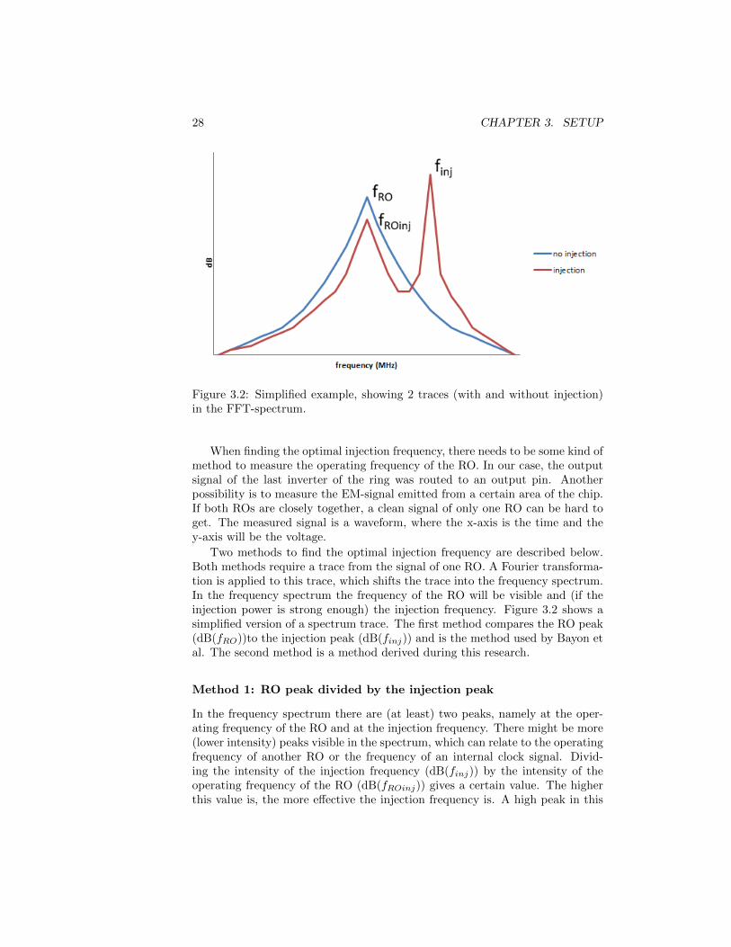
Figure 3.2: Simplified example, showing 2 traces (with and without injection)in the FFT-spectrum.

When finding the optimal injection frequency, there needs to be some kind ofmethod to measure the operating frequency of the RO. In our case, the outputsignal of the last inverter of the ring was routed to an output pin. Anotherpossibility is to measure the EM-signal emitted from a certain area of the chip.If both ROs are closely together, a clean signal of only one RO can be hard toget. The measured signal is a waveform, where the x-axis is the time and they-axis will be the voltage.

Two methods to find the optimal injection frequency are described below.Both methods require a trace from the signal of one RO. A Fourier transforma-tion is applied to this trace, which shifts the trace into the frequency spectrum.In the frequency spectrum the frequency of the RO will be visible and (if theinjection power is strong enough) the injection frequency. Figure 3.2 shows asimplified version of a spectrum trace. The first method compares the RO peak(dB(fRO))to the injection peak (dB(finj)) and is the method used by Bayon etal. The second method is a method derived during this research.

Method 1: RO peak divided by the injection peak

In the frequency spectrum there are (at least) two peaks, namely at the oper-ating frequency of the RO and at the injection frequency. There might be more(lower intensity) peaks visible in the spectrum, which can relate to the operatingfrequency of another RO or the frequency of an internal clock signal. Divid-ing the intensity of the injection frequency (dB(finj)) by the intensity of theoperating frequency of the RO (dB(fROinj)) gives a certain value. The higherthis value is, the more effective the injection frequency is. A high peak in this

3.4. VERIFICATION METHODS 29

spectrum signifies more activity on a given frequency. If the injection frequencypeak is higher than the operating peak of the RO (which is the measured signal),the RO might have locked to this injection frequency.

Method 2: RO peak during injection substracted from the RO peakwithout injection

This method requires two cases. One case is a measurement without injection.The second case should be taken during injection. As mentioned before, a highpeak in the frequency spectrum signifies a high activity on that frequency. To seewhether ROs might have been locked to a frequency different from the originalfrequency, one can also measure the y-value of a peak in the spectrum at twodifferent points in time. This method only looks at the height of the peak of theoperating frequency of the RO. If the peak of the operating frequency of the ROduring injection (dB(fROinj)) is lower than the peak when no injection is done(dB(fRO)), it can be concluded that the RO has less activity on that frequencyand locked to another frequency. An optimal injection frequency would then bethe lowest value. Although this method is not described in the current literature,Section 5.2 shows that it yields similar results.

3.4.2 Mutual information

While the above methods aim to find an optimal injection frequency, this doesnot mean that an attack on the found injection frequency works. In order toverify that the injection frequency locked the ROs another measure is used:mutual information. Mutual information calculates the information in bits thatis shared among two different entities, in this case ROs. When the optimalinjection frequency is found, it can be verified using mutual information. Mutualinformation needs measurements of two ROs. These measurements are thevoltage usage of the element of the ring that is connected to the harvestingmechanism. It gets the voltage level of these two measurements at a givensampling speed (10 GHz for example) and divides these points into a certainamount of bins. The mutual information is calculated from these bins. If themutual information is (close to) zero, the two ROs are independent from eachother. Mutual information is upper bounded by the minimum entropy of theamount of bins.

This research divided the different sampling points into four equally sizedbins. For every trace the maximum and the minimum voltage level was acquired.The minimum was substracted from the maximum and divided by the numberof bins (4 bins in this research). This gives the size for every bin. The firstbin would thus be in the range [minimum,minimum+ 1 ∗ size], bin two wouldbe in the range [minimum,minimum + 2 ∗ size] etcetera. Once all the tracesare processed and the points from the traces are divided into the bins, themutual information is calculated. In this research the mutual information isupper-bounded by 2. If the mutual information is 2, the ROs are completely

30 CHAPTER 3. SETUP

interdependent and thus locked onto the same frequency. This means that theoutput of the TRNG should be completely biased.

3.4.3 Random number test suites

A definite way to check if the attack succeeded is to check the random numberproduced by the system. The NIST monobit test and block frequency test wereused to check if the attack succeeded. The reasoning is that if two rings havea high mutual information, the resulting XOR-tree will produce a lot of zeroes.These zeroes are sampled, gathered into a binary file and fed as input to thetest-suite. A test-suite should be able to determine if the fault injection wassuccessful at biasing the TRNG based on the monobit-test. In order to accountfor temporary effects, a block frequency test was also used. If there are certainblocks that contain a lot of zeroes (or ones), this test should be able to findit. Other random number test suites like Dieharder and AIS-31 were also used.The advantage of the NIST test-suite is the low amount of bits required to runthe tests, thus having fast results.

Chapter 4

Initial experiments on aTRNG

This chapter describes an initial experiment to monitor the effects of an EM-FIusing harmonic emission on the RO-based TRNG running on the Actel FusionFPGA. The operating frequency of an RO is primarily determined by the ele-ments of the ring and the wires connecting it. Fluctuations on this operatingfrequency can be induced by the temperature and the injected frequency. Dur-ing a FI the temperature of the FPGA rises. Reasons for this are the heat ofthe amplifier that is blown on top of the FPGA, but also the electric coupling inthe FPGA induced by the injected signal. This experiment aims to identify theeffect of the FI on the operating frequencies of the ROs. First some architec-tural decision that were made will be elaborated, followed by the experimentsand results. A conclusion will summarize the results for this experiment.

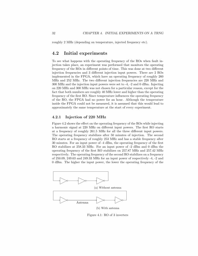
4.1 Design

In order to have more effect on the ROs, an antenna was introduced in everyRO. The distance between the first and second element of a RO in the TRNGwas made larger. Due to this distance, a long wire connected these elements. Itis assumed that a RO with this long wire is influenced easier than a RO withouta long wire since the area of impact is larger. Figure 4.1 shows an example ofa RO with and an RO without an antenna. A disadvantage of this antenna isthe drop of operating frequency it causes. A lower frequency means less effecton the RO because the electric coupling behaves less effective.

For the next experiments, the ROs consisted of 3 elements. Without anantenna, the operating frequency of the RO would be in the window [320−330]MHz. With the antenna, the operating frequency drops to [240 − 260] MHz.This large window is based on the routing specifications of the FPGA that itimplements and the optimum positioning of all the elements of the design. Oncea RO is placed and routed, the operating frequency of the RO can change with

31

32 CHAPTER 4. INITIAL EXPERIMENTS ON A TRNG

roughly 2 MHz (depending on temperature, injected frequency etc).

4.2 Initial experiments

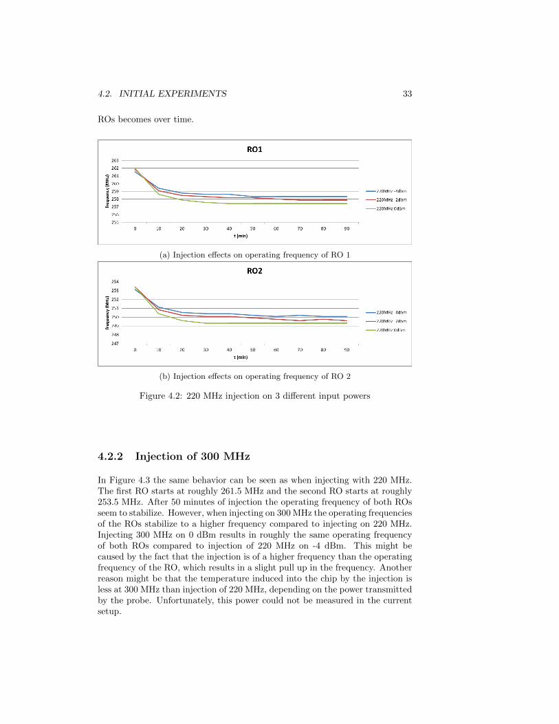
To see what happens with the operating frequency of the ROs when fault in-jection takes place, an experiment was performed that monitors the operatingfrequency of the ROs in different points of time. This was done at two differentinjection frequencies and 3 different injection input powers. There are 2 ROsimplemented in the FPGA, which have an operating frequency of roughly 260MHz and 252 MHz. The two different injection frequencies are 220 MHz and300 MHz and the injection input powers were set to -4, -2 and 0 dBm. Injectingon 220 MHz and 300 MHz was not chosen for a particular reason, except for thefact that both numbers are roughly 40 MHz lower and higher than the operatingfrequency of the first RO. Since temperature influences the operating frequencyof the RO, the FPGA had no power for an hour. Although the temperatureinside the FPGA could not be measured, it is assumed that this would lead toapproximately the same temperature at the start of every experiment.

4.2.1 Injection of 220 MHz

Figure 4.2 shows the effect on the operating frequency of the ROs while injectinga harmonic signal at 220 MHz on different input powers. The first RO startsat a frequency of roughly 261.5 MHz for all the three different input powers.The operating frequency stabilizes after 50 minutes of injection. The secondRO starts at a frequency of roughly 253 MHz and has a stable frequency after30 minutes. For an input power of -4 dBm, the operating frequency of the firstRO stabilizes at 258.33 MHz. For an input power of -2 dBm and 0 dBm theoperating frequency of the first RO stabilizes on 257.87 MHz and 257.42 MHzrespectively. The operating frequency of the second RO stabilizes on a frequencyof 250.09, 249.63 and 249.33 MHz for an input power of respectively -4, -2 and0 dBm. The higher the input power, the lower the operating frequency of the

(a) Without antenna

Antenna

(b) With antenna

Figure 4.1: RO of 3 inverters

4.2. INITIAL EXPERIMENTS 33

ROs becomes over time.

(a) Injection effects on operating frequency of RO 1

(b) Injection effects on operating frequency of RO 2

Figure 4.2: 220 MHz injection on 3 different input powers

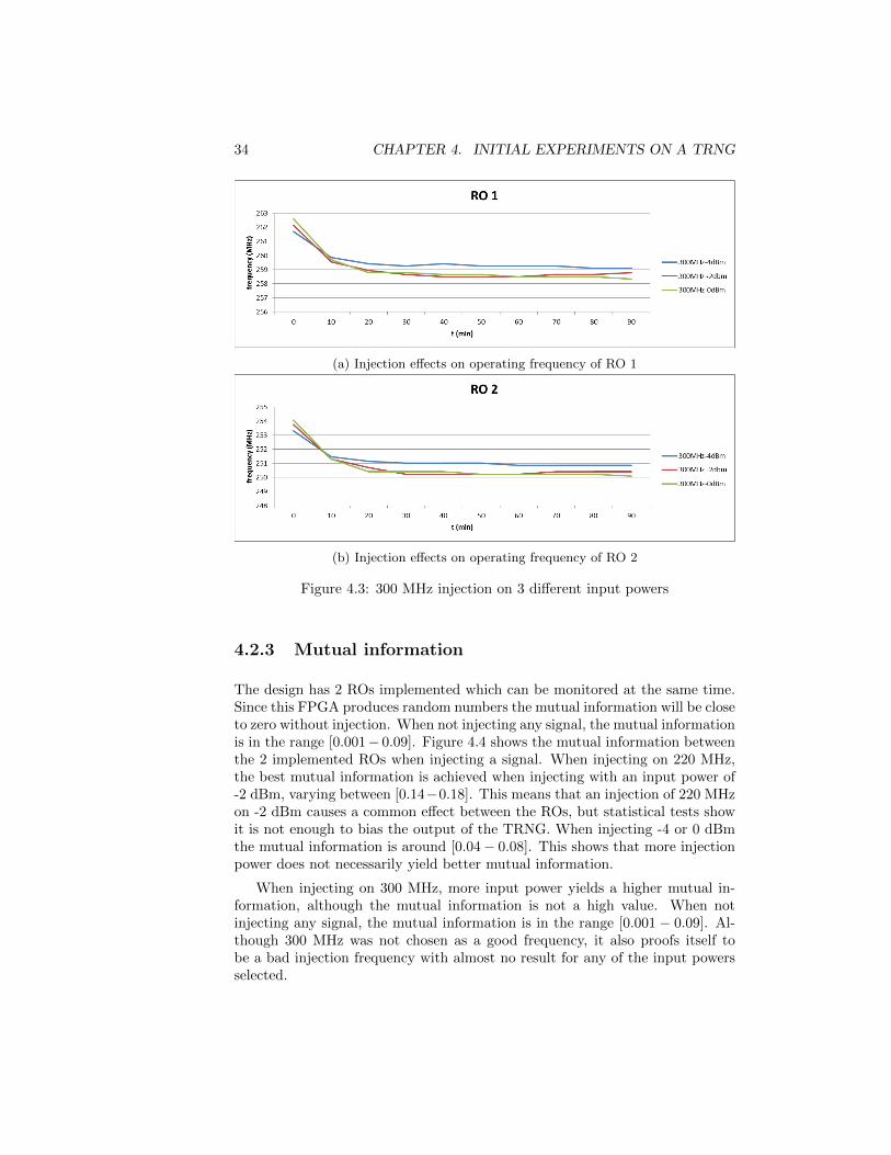
4.2.2 Injection of 300 MHz

In Figure 4.3 the same behavior can be seen as when injecting with 220 MHz.The first RO starts at roughly 261.5 MHz and the second RO starts at roughly253.5 MHz. After 50 minutes of injection the operating frequency of both ROsseem to stabilize. However, when injecting on 300 MHz the operating frequenciesof the ROs stabilize to a higher frequency compared to injecting on 220 MHz.Injecting 300 MHz on 0 dBm results in roughly the same operating frequencyof both ROs compared to injection of 220 MHz on -4 dBm. This might becaused by the fact that the injection is of a higher frequency than the operatingfrequency of the RO, which results in a slight pull up in the frequency. Anotherreason might be that the temperature induced into the chip by the injection isless at 300 MHz than injection of 220 MHz, depending on the power transmittedby the probe. Unfortunately, this power could not be measured in the currentsetup.


(a) Injection effects on operating frequency of RO 1

(b) Injection effects on operating frequency of RO 2

Figure 4.3: 300 MHz injection on 3 different input powers

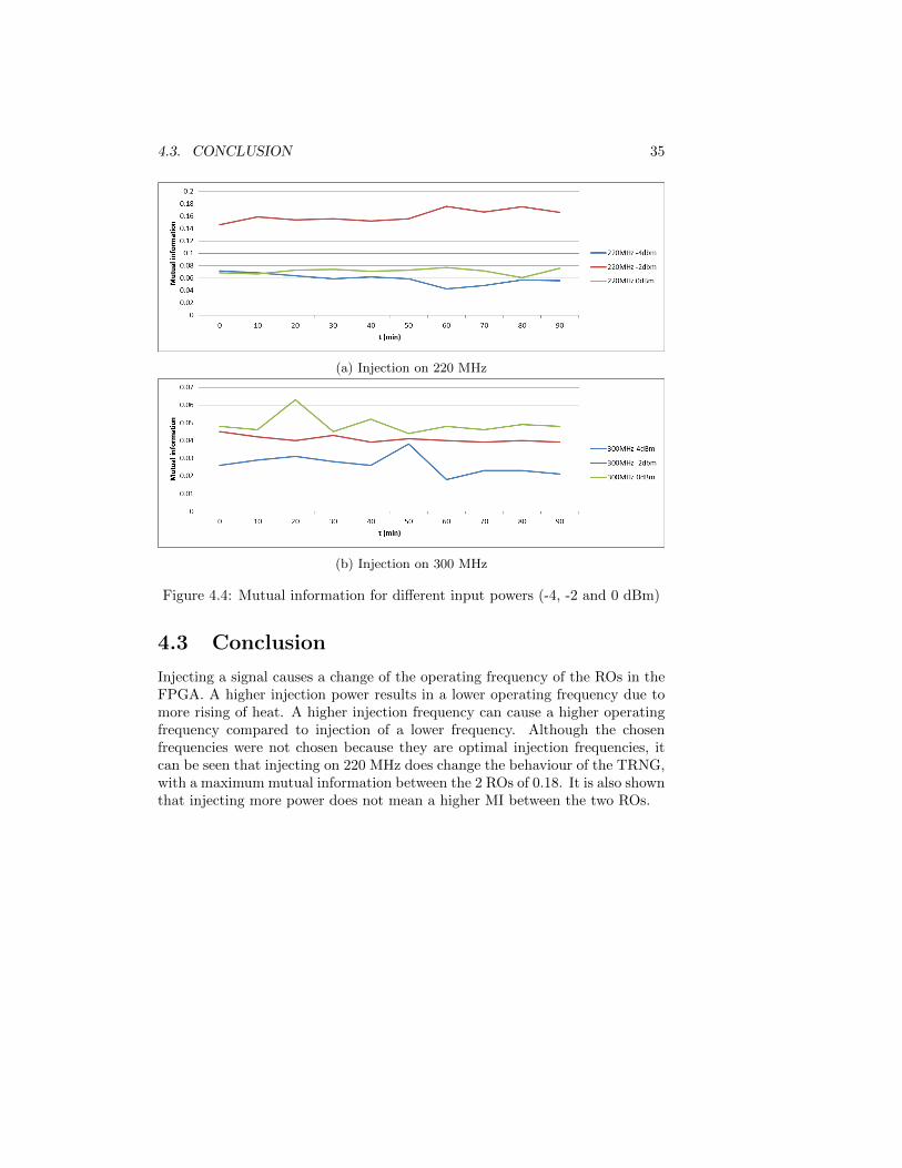
4.2.3 Mutual information

The design has 2 ROs implemented which can be monitored at the same time.Since this FPGA produces random numbers the mutual information will be closeto zero without injection. When not injecting any signal, the mutual informationis in the range [0.001− 0.09]. Figure 4.4 shows the mutual information betweenthe 2 implemented ROs when injecting a signal. When injecting on 220 MHz,the best mutual information is achieved when injecting with an input power of-2 dBm, varying between [0.14−0.18]. This means that an injection of 220 MHzon -2 dBm causes a common effect between the ROs, but statistical tests showit is not enough to bias the output of the TRNG. When injecting -4 or 0 dBmthe mutual information is around [0.04 − 0.08]. This shows that more injectionpower does not necessarily yield better mutual information.

When injecting on 300 MHz, more input power yields a higher mutual in-formation, although the mutual information is not a high value. When notinjecting any signal, the mutual information is in the range [0.001 − 0.09]. Al-though 300 MHz was not chosen as a good frequency, it also proofs itself tobe a bad injection frequency with almost no result for any of the input powersselected.

4.3. CONCLUSION 35

(a) Injection on 220 MHz

(b) Injection on 300 MHz

Figure 4.4: Mutual information for different input powers (-4, -2 and 0 dBm)

4.3 Conclusion

Injecting a signal causes a change of the operating frequency of the ROs in theFPGA. A higher injection power results in a lower operating frequency due tomore rising of heat. A higher injection frequency can cause a higher operatingfrequency compared to injection of a lower frequency. Although the chosenfrequencies were not chosen because they are optimal injection frequencies, itcan be seen that injecting on 220 MHz does change the behaviour of the TRNG,with a maximum mutual information between the 2 ROs of 0.18. It is also shownthat injecting more power does not mean a higher MI between the two ROs.


Chapter 5

TRNG implemented with 5ROs

The amplifier used for these experiments was new. The effects induced by thisamplifier was not yet investigated. Chapter 4 shows that the amplifier injectsa signal and changes the behavior of the TRNG. This Chapter will describe areplication of the research performed by Bayon et al. in order to verify thatthe amplifier can bias a RO-based TRNG. We will first discuss the slightlydifferent RO-based TRNG design compared to the research by Bayon et al.,followed by a frequency sweep. Afterwards the mutual information will beshown, followed by some power sweeps on some of the best frequencies basedon the mutual information. Then the test results of the NIST test suite will beshown, together with visual representations of the random number. The lastsection will be a conclusion based on these results. Appendix D describes someadditional experiments performed with a smaller and isolated probe.

5.1 Design

Figure 5.1 shows the layout of the ROs of the TRNG for this experiment. Thereare 5 ROs implemented in this design, all placed horizontal with some spacebetween the ROs. They are placed towards the left part of the chip (within thered circle) to prevent influencing other parts of the design (like the XOR-treeand the FIFO queue and the registers) during the injection. The top horizontalrow is the first RO, the second row the second RO etc. Although there is somespace in-between the ROs, it might still be possible that cross-talk happensbetween the antennas of the ROs. To be able to influence all the ROs it waschosen to keep the ROs close together, but far enough to prevent interlockingof the ROs without any injection. The implemented design passes all tests fromthe NIST SP-800 test-suite with a file of 1 GB.

The operating frequencies of the ROs of this design are shown in Table 5.1.As shown before, this operating frequency changes due to temperature and the

37

38 CHAPTER 5. TRNG IMPLEMENTED WITH 5 ROS

RO nr. Frequency(MHz)

1 2422 2483 2554 2415 241

Table 5.1: Rough estimation of the operating frequencies of the ROs.

Figure 5.1: Design consisting of 5 ROs of length 3, all with an antenna

introduced fault injection.

5.2 Frequency sweep

To find the optimal injection frequency a frequency sweep was done. Section3.4.1 describes 2 methods to finds the optimal injection frequency. The firstmethod divides the intensity of the injection peak by the intensity of the peakof the operating frequency of the RO. The second method substracts the inten-sity of the peak of the operating frequency during injection by the intensity ofthe peak of the operating frequency without injection. Both methods will bediscussed below.

Figure 5.2 shows the results for dividing the peak of the operating frequencyof the RO by the injection peak. Figure 5.3 shows the sum of all the resultsof the ROs. The left side of the frequency spectrum has no to little effect, butthere is an optimum towards the right side of the spectrum. After 278 MHzthe optimum seems to decrease again. Table 5.2 shows the top 10 optimuminjection frequencies according to this method.

Table 5.3 shows the top 10 best results for the second method. There seemsto be some optimum around 257 MHz to 259 MHz. The best injection frequency

5.2. FREQUENCY SWEEP 39

Figure 5.2:dB(finj)dB(fRO) for every implemented RO of the TRNG


Figure 5.3: Sum of thedB(finj)dB(fRO) values

Nr. finjdB(finj)dB(fRO)

1 269.3 80.16462 275.4 78.023873 269.6 76.791034 270.2 76.655765 278.6 76.325586 269.45 74.507227 272.95 73.658418 274.05 71.452379 274.35 70.8036910 274.5 70.36323

Table 5.2: Top 10 best results for dividing the injection peak by the peak of theoperating frequency of the RO.

is 248.6 MHz, which is the exact operating frequency of RO2 at that time. The9th best injection frequency is 255.45 MHz, which was the operating frequency ofRO3 at that point in time. The 3rd best injection frequency is 269.6 MHz, whichwas also the third best injection frequency in the previous methods. When goingthrough a larger set of the results, there seems to be more overlap between thedifferent verification methods (e.g. an injection of 257.85 MHz is the 25th bestinjection frequency for the first method and the second best injection frequencyfor the second method).

Several candidates for an optimal injection frequency have been chosen andare listed below:

• 228.5 MHz

• 248.6 MHz

• 257.85 MHz

• 269.3 MHz

• 269.45 MHz

• 269.6 MHz

• 275.4 MHz

5.3. MUTUAL INFORMATION 41

Nr. finj dB(fROinj) − dB(fRO)1 248.6 -25.60372 257.85 -24.6283 269.6 -22.22554 235.25 -21.37345 228.5 -18.27886 258.5 -17.75117 258.85 -16.3858 228.05 -16.35449 255.45 -15.648710 258.8 -14.8368

Table 5.3: Top 10 best results for substracting the RO peak during injection bythe RO peak without injection

The best three injection frequencies for both methods were chosen. In addi-tion to these, the injection frequency 269.45 MHz was chosen because it appearsin the top 10 and is exactly in between 269.3 MHz and 269.6 MHz, which areboth in the top 3 in the first method. Furthermore, injection of 228.5 MHzproduces 5 negative values for the second method, implying that all the ROshave locked to a different frequency and might have interlocked. The next Sec-tion will continue with a small power sweep for the different candidates. Duringthese power sweeps, the MI between two ROs was measured.

5.3 Mutual information

A small power sweep was performed on the previously described candidates asoptimal injection frequencies. During the power sweep the mutual informationbetween 2 ROs was calculated. The power sweep ranged from -2 dBm to 0dBm, with a step size of 1 dBm. This was done for every pair of ROs (thus 10measurements for every different input power injection). Figure 5.4 shows theaverage result of all the power sweeps on the different input power injections.Figure 5.4 also shows some initial mutual information of 0.1 to 0.2. This isbecause RO1, RO4 and RO5 seem to be interlocking without injection takingplace. This could be caused by the fact that their operating frequencies are closeto each other and some cross-talk between the introduced antennas in the ROs.Although the ROs are not completely independent, the output of the TRNGwas still statistically random.

Figure 5.4 clearly shows that injection of a frequency at -2 dBm increasesthe mutual information between the ROs with respect to no injection. For allthe chosen injection frequencies the MI goes up during injection compared tono injection. The best injection frequency (of the chosen injection frequencies)seems to be 257.85 MHz, reaching a maximum MI of 0.46 bits. From Figure 5.4it also seems like more power does yield a higher MI, although this shouldn’t


Figure 5.4: Averages of every MI between 2 ROs for all the chosen frequencies

necessarily be the case (see Figure 4.4).

5.4 Power sweep

A larger power sweep was performed on an injection of 257.85 MHz. The powersweep ranged from -8 dBm to 0 dBm with a step-size of 1 dBm. Figure 5.5shows the MI for every couple of ROs. As can be seen, RO1 and RO5 arealready interlocked with an MI of 0.73 without injection. Nevertheless, injectiondoes increase the MI between the two ROs even more. Getting a high mutualinformation between RO2 and RO3 appears to be the most difficult objective,although a high MI between RO2 and RO3 also seems hard. The chosen injectionfrequency seems to lock most of the ROs, but seems to be less effective for RO2in combination with RO3 and RO4.

Injection with an input power of -4 dBm seems to enhance the MI betweenRO1 and RO5, but decreases the MI between RO1 and RO4. It therefore seemsthat different powers might work better for 2 ROs, while performing worse forothers. In general, more power does seem to increase the MI between 2 ROs.Since it was shown in Figure 4.4 that this is not necessarily true, the measuredMI started to become doubtful. It could be possible that the LeCroy probesmeasured the signal of the injected signal over the air in conjunction with thesignal of the ROs. However, this noise coming over the air should not have ansignificant effect on the measured signal of the ROs. Nevertheless, we decidedto shield the LeCroy probes with some aluminum foil for the next experimentsto prevent measuring this noise as much as possible.

5.5. RNG TEST SUITE RESULT 43

Figure 5.5: The MI during a power sweep on 257.85 MHz

5.5 RNG test suite result

A file of 1 GB of the output of the TRNG was gathered during injection of257.85 MHz with an input power of -2 dBm. Note that it passed all the NIST-tests without any fault injection with the same size. The TRNG failed all theNIST-tests (including the monobit test) with the file that was taken during theinjection. However, although 1.4% of the random number was biased in themonobit test, a visual inspection lacks a result comparable with those shownby Bayon et al.. Figure 5.6 shows the maximum bias as the visual result, withthe bit zero drawn as a white square and the bit one drawn as a black square.The number drawn consists of 3840 (60 x 64) bits. The maximum bias achievedtowards ones is 7.3% (2062 of the total amount of 3840 bits are 1’s) and themaximum bias achieved towards zeroes is 8.0% (2074 bits of the total amountof 3840 bits are zeroes). For comparison, Figure 5.7 shows the results achievedby Bayon et al. at different output powers (PForward). This PForward is thepower emitted by the probe and is a different power than the input power usedin this thesis, as explained in Chapter 3. The research done by Bayon et al.achieved a bias of 55% towards zeroes. It might be possible that the injectedsignal is directly picked up by the LeCroy probes, instead of propagated overthe signal of the ROs.

5.6 Conclusion

This experiment was a full replica of the research performed by Bayon et al.Although a high mutual information was achieved and the TRNG becomesbiased (failing the NIST monobit test), a visual results like those presented byBayon et al. were not achieved. Although the visual results are not comparablewith those achieved by Bayon et al., good confidence was found in the MI whichshows that the ROs were mutually interlocked. The following experiments willhave an aluminum foil wrapped around the LeCroy probes, to prevent themfrom measuring the injection signal as noise over the air. This should make itpick up none to low noise of the injection directly onto the LeCroy probe. The


(a) (b)

Figure 5.6: Visual representation (0’s in white, 1’s in black) of the maximumbias towards ones (Figura (a): 7.3%) and towards zeroes (Figure (b): 8.0%)

Figure 5.7: Results achieved by Bayon et al. [6]

5.6. CONCLUSION 45

rest of the research will continue to base its results on MI.


Chapter 6

Injection on differentimplementation designs

Although the experiment described in Chapter 5 showed promising results, re-production of the experiment seemed to be hard and sometimes impossible.Therefore, to be able to study the exact effect of the FI on the ROs, we decidedto implement a TRNG using only 2 ROs. This does not only make it possible tomonitor all the entropy sources of the TRNG, but also makes the experimentsmore time-efficient. Calculating the MI of a TRNG using only 2 ROs requiresonly 1 measurement, while a TRNG of 5 ROs requires 10 measurements (onefor each pair of ROs). The first section will describe the initial experiment per-formed, building up to the main research described in Section 6.2. Section 6.2will describe possible designs in detail with the experiments performed on them.The sections afterwards will go into more detail for the designs and discuss theresults.

6.1 Initial experiment

Having a design of 2 ROs makes it possible to calculate the MI during thefrequency sweep, thus skipping the step to find the optimum injection frequency.The next experiment did a frequency sweep and analyzed the MI to find a goodinjection frequency. This experiment had an initial injection position slightlyaway from the location of the ROs (unintentionally) and an unexpected resultwith a maximum MI of 0.1. A second sweep was done, positioned right on top ofthe ROs, yielding better results. It seemed that the location was influencing theresult. Therefore, 4 additional frequency sweeps were done. The first frequencysweep was performed on top of the ROs. The other four frequency sweeps werelocated in the corners of the chip.

47

48CHAPTER 6. INJECTION ONDIFFERENT IMPLEMENTATION DESIGNS

Figure 6.1: Frequency sweep located on top of the ROs

Figure 6.2: Frequency sweep located in the top left corner of the chip

6.1.1 Frequency sweep & mutual information

The frequency sweep ranged from 180 MHz to 280 MHz with a step-size of 50KHz and a injection input power of -2 dBm. Figure 6.1 shows the frequencysweep with the probe located on top of the ROs. Figure 6.2 shows the frequencysweep with the probe located in the top left corner of the chip. The otherfrequency sweeps can be found in Appendix C. From Figure 6.1 it can be seenthat there is some optimum around 202 MHz after which the MI starts dropping.After 237 MHz the MI starts to increase again, with 5 peaks. The peaks are at249.3 MHz, 250.45 MHz, 250.95 MHz, 254.7 MHz and 259 MHz. From these 5peaks, at the time the measurements were taken the second peak correspondsto the operating frequency of the first RO, the fourth peak corresponds to themean of the operating frequencies of both ROs, and the fifth peak correspondsto the operating frequency of the second RO. Figure 6.2 shows similar behavioras Figure 6.1. Some optimum at 202 MHz and several peaks towards the right.At the time those measurements were taken, the first RO had an operatingfrequency of 250.2 MHz and the second RO had an operating frequency of 258.55MHz. The first peak is indeed on the operating frequency of the first RO, thesmaller peak in between the larger peaks is the mean of the frequencies, andthe largest peak is the operating frequency of the second RO. All measurements(see Appendix C) show this behavior, with a peak at the operating frequencyof the RO and the mean of the operating frequencies.

6.2. DESIGNS 49

It seems that injecting on the operating frequency of the RO seems to be agood way to achieve a high mutual information. Also, the value of the MI differsbetween the different injection locations. Injecting on top of the ROs achieved amaximum MI of 0.47, while injecting in a corner (outside of the programmabledie of the chip, see Figure 6.3) achieves a maximum MI of 0.82. This showsthat injecting with the operating frequency of the implemented ROs seems tobe a very efficient way to interlock the ROs, but the maximum value of MI alsoseems to depend on the location of the injection. Note that the MI is purelybased on the signal of the ROs, since the probes are shielded and should notmeasure any noise (or at the least should have a very low noise-level).

6.2 Designs

To make it easier to determine the effect on the ROs, several designs werechosen of a TRNG with only 2 ROs. Although the introduced antenna in theROs is assumed to enhance the effect, it is not yet investigated to be true. Thissection will thus also aim to elaborate on the effect of the antenna. Since theeffectiveness of the injection also seems to be dependent on the location of theinjection, an area to do an XY-scan is defined first.

6.2.1 Scanning area

In order to see the effect of different locations of injection, an area was definedto perform an XY-scan on. To know what area to scan, the actual size of thedie of the chip needs to be known. Since the FPGA had to be returned to theprevious owner, decapitation of the chip was not an option. Therefore a designwas created with 2 different ROs with 2 very different operating frequencies.One RO was put in the bottom left corner and one RO was put in the upperright corner. Hovering over the chip with an EM-probe can pick up the signalemanating from the chip. The LeCroy can calculate the FFT spectrum fromthat signal on the spot and by looking at the spectrum it is known wherethe RO is located. Although this method is not very precise, it does give anapproximation of the size of the programmable die. Although there is more inthe chip than just the programmable die, it does give an approximation on thepoint of injection and might give some insight in the areas the FI is affecting.

The approximate size of the programmable die is shown in Figure 6.3(bluerectangle). The scan was performed on the chip which was rotated 90 degreescounter-clockwise. The chip was also mirrored (or up-side-down). The ROswere placed in the bottom left corner (blue dot in Figure 6.3), and the scan areawas a 15x15 grid around the placement of the implemented ROs (red rectanglein Figure 6.3). Note that these areas are not precise (both the programmabledie area as the scan area), but is merely an indication of the areas that willbe talked about in the next experiments. The XY-scan starts from the top leftcorner towards the bottom right corner. The ROs will be located near the 8throw and the 5th column in the scanned grid-area.


Figure 6.3: The chip and its programmable die (blue rectangle), location of theROs (blue dot) and the scan area (red rectangle)

6.2.2 The chosen designs

There are several ways to implement a TRNG based on ROs. A design thatimplements the ROs in a horizontal orientation results in different frequenciesthan a design that implemented the ROs in a vertical orientation. This differencein operating frequency can be as large as 20 MHz. An artificial antenna wasalso introduced between the first and second element of the RO. The effect ofthis antenna can also be tested in comparison with a design that does not havethis antenna. The way the ROs are organized can also influence the outputof the TRNG. If ROs are placed parallel to each other, crosstalk might occurbetween the ROs. A design that has the ROs in-line might suffer less from thecrosstalk. Another design choice is to change the length of the ROs. For thenext experiments, the designs that have an unequal ring length will consist of 3inverters for the first RO and 5 inverters for the second RO. For every design thathas an unequal length in combination with an antenna results in an antenna forthe first (3 inverter) RO only. The main reason for this design choice is that theantenna results in operating frequencies that are closer together. The surfaceof a RO of length 5 is also bigger and almost equal to that of a RO of length 3with an antenna. The list below summarizes the different designs that will betested and will be elaborated in the next sections. All these different designsare done in combination with each other, resulting in (2x2x2x2=) 16 differentdesigns.

• The different between a horizontally placed ROs and vertically placedROs.

• With and without an antenna between the first and second element of theRO.

• Placing the ROs parallel to each other or in sequence with each other.

6.2. DESIGNS 51

• ROs of different ring length, where one RO has a length of 3 elements inand the second RO has a length of 5 elements.

6.2.3 Flow of an experiment

For each design mentioned, an XY-scan over an area of the die of the chip asdisplayed in Figure 6.3 (red rectangle) is performed. The area is divided intoparts of 15 by 15 and thus gives 225 measurements per experiment. The area isscanned three times for one injection frequency and 3 injection frequencies werechosen. The injection frequency is dynamically calculated and corresponds tothe frequency of the first RO, the frequency of the second RO and the meanfrequency of the ROs.

Every experiment followed the following procedure:

1. Acquire two traces from the LeCroy, corresponding to a trace for the firstRO and the second trace for the second RO. These traces are taken withoutany injection performed.

2. From the 2 gathered traces from step 1, calculate the FFT for each. Theoperating frequency of the first RO can be calculated from this first FFTtrace. The operating frequency of the second RO can be calculated fromthe second FFT trace. The operating frequency of the RO is the x-valuewhere the highest peak of the trace is. Based on the chosen mode, theinjection frequency is chosen. This is either the operating frequency ofthe first RO, the operating frequency of the second RO or the mean ofboth frequencies. The injection frequency is communicated to the signalgenerator and the amplifier is turned on.

3. Acquire two traces from the LeCroy, where the first trace corresponds tothe first RO and the second trace to the second RO. These traces will betaken while there is an injection taking place.

4. Turn the amplifier off and go to the next position of the XY-scan. Repeatthe process from step 1.

Due to temperature changes and the injection done for the previous location,the frequency of the ROs changes. This is the reason why the frequency of theRO needs to be calculated again for every location. The temperature changesmight be environmental changes (e.g., heat emitted by the amplifier), but alsotemperature changes induced by our injection which causes a higher temperaturein the chip itself because of electric coupling. This workflow makes it possibleto inject a frequency that is close to equal to the operating frequency of eitherRO.

For every experiment, the mutual information is calculated and put intoan XY-plot. The different coloring of the squares represents the amount ofmutual information. The scaling of these colors will be elaborated on in eachexperiment. A dark red square represents the highest MI achieved during theexperiment. A dark blue square represents the lowest measured MI.


Figure 6.4: Horizontal, without antenna, in-line, equal length. Average of 3XY-scans with an injection of the frequency of the second RO

6.3 General remarks

The average of the 3 XY-scans for an injection frequency for every design canbe found in Appendix E. Appendix E will discuss every design separately. Thissection will continue with some general remarks and give some conclusion onthe effects of using the different designs.

Figure 6.4 shows the average result of three XY scans with an injection ofthe operating frequency of the second RO. The maximum achieved MI is 0.138at spot (2,6). The ROs are located at spot (8,5) and the maximum is thus notreached on top of the ROs. However, spots with some of the highest MI duringthis experiment, namely (2,6), (4,5), (1,7) and (4,8), are all located near thewire that goes from the third inverter element to the XOR-gate. Influencingthe wire going to the harvesting mechanism can thus also affect the ROs andpropagates the injected signal backwards into the ROs.

Another result of the average of a frequency injection equal to the operatingfrequency of the second RO is shown in Figure 6.5. The ROs in this designwere placed horizontal, without an antenna, inline of each other and of unequallength. This result also has some high MI values near the wire going towardsthe harvesting mechanism (from (8,5) to (0,9)). However, there are also high MIvalues in the 10th and 11th row. These high MI values might give a wrong idea,since this could be an influence on the bonding wire going from the selectedoutput pin in the chip towards the output pin to which the LeCroy probes are

6.3. GENERAL REMARKS 53

Figure 6.5: Horizontal, without antenna, in-line, unequal length. Average of 3XY-scans with an injection of the frequency of the second RO

attached. It can also be possible that these bonding wires were influenced andthe signal propagated backwards into the ROs (as is the case for the wire going tothe harvesting mechanism) and did influence the ROs. A definitive conclusionon this cannot be given, but could be tested by monitoring and testing theoutput of the TRNG.

Another conclusion drawn from Figure 6.5 is that the location of the injectionmatters a lot. An injection with the operating frequency of RO2 at spot (4,12)results in an average MI of 0.6, while a location slightly above it ((3,12)) yieldsa MI of 0.1 and is thus ineffective. The importance of this location dependentsuccess is one of the reasons for not being able to replicate results from previousexperiments. Indeed, before doing the experiment of Section 6.1 it was believedthat the effect of an injection was a global effect. This research shows that thisis not the case and that it is a local effect when injecting a frequency equal tothe operating frequency of the ROs. When injecting the mean of the operatingfrequencies, it does seem to be a more or less global effect.

The ROs of unequal length are believed to produce better results since thefrequency difference is larger and mutual interlocking is harder to achieve. Al-though this design does not produce a statistical random number, it does passthe monobit-test from the NIST test-suite. Also, the mutual information be-tween the 2 ROs is between 0.01 and 0.18 without injection, while the mutualinformation for equal length ROs is between 0.01 and 0.09.

Using a design that has vertically parallel placed ROs of equal length without


an antenna seems to be the most insusceptible to this attack, with a maximumMI of 0.08, which is equal to some measurements without injection. This designdoes show that the top right corner of the scanned area is influenced more thanthe rest of the chip. Although no definitive reason for this effect can be given,there might be something that is connected to the ROs. It could be possiblethat there might be a power supplier for the FPGA near that spot, which mightpropagate the signal over the power net into the ROs. Unfortunately this cannotbe proven and is merely one guess among many possible options.

Injecting on the operating frequency of RO2 seems to be more effectivethan injecting the operating frequency of RO1. Exception to this rule are thedesigns placed horizontal, with antenna in parallel of unequal length and verticalwith antenna, inline and unequal. Common factor between these designs is theunequal ring length and both have an antenna. For the second design however,the MI went up to 0.42 which is also a good result. The first design had a MIof 0.09 when injecting the operating frequency of RO2, which can be seen asineffective.

6.4 Horizontal vs vertical placement

The assumption is that the placement of the RO in a horizontal or verticalorientation will not differ in the results. This seems to be correct, althoughthere might to a relation with the implemented antenna. The next section willdiscuss this relation.

6.5 With antenna vs without antenna

We assume that the antenna introduced between the first and second elementof the RO will yield better results. As pointed out in Section 6.3, the wire goingto the harvesting mechanism can also act as an antenna. The wire going tothe harvesting mechanism is longer than the wire introduced inside the RO(s).Although electric coupling might be less on the lower frequency resulting fromthe antenna between the first and second element of the RO, it is still believedthat this antenna should yield better results. The experiments show that thisis not always correct. For the design that had the ROs placed vertical with anantenna generally had a higher result than the designs without an antenna. Theopposite is true for horizontal placed ROs, where horizontal designs without anantenna generally achieved higher MI than those with an antenna. There is anexception to this, namely the design with ROs placed vertical, parallel and anunequal length. In that case the design without the antenna performs betterwhen injecting the mean operating frequency of the ROs. Table 6.1 shows themaximum achieved average for each design.

Table 6.1 also shows that the use of an antenna in a RO of unequal lengthdoes not make it more influencable. Although RO1 (the RO of length 3) wasthe only RO with the antenna, these cases do not always show a higher MI than

6.6. INLINE VS PARALLEL PLACEMENT 55

the same design without an antenna (and vice versa).

with antenna without antennafRO1 fRO2 fmean average fRO1 fRO2 fmean average

horizontal,inline, equal

0.08 0.11 0.12 0.10 0.09 0.15 0.06 0.10

horizontal,inline, unequal

0.34 0.36 0.07 0.26 0.31 0.64 0.37 0.44

horizontal, par-allel, equal

0.14 0.21 0.09 0.15 0.19 0.23 0.07 0.16

horizontal, par-allel, unequal

0.52 0.09 0.07 0.23 0.26 0.49 0.33 0.36

vertical, inline,equal

0.18 0.37 0.20 0.25 0.05 0.18 0.03 0.09

vertical, inline,unequal

0.72 0.42 0.06 0.40 0.08 0.57 0.07 0.24

vertical, paral-lel, equal

0.23 0.46 0.21 0.30 0.01 0.09 0.01 0.04

vertical, paral-lel, unequal

0.36 0.55 0.07 0.33 0.19 0.44 0.65 0.43

Table 6.1: Design comparisons between ROs with antenna and without antennabased on MI

6.6 Inline vs parallel placement

Parellel implemented ROs can have some crosstalk between the ROs, while ROsthat are placed in-line suffer less from crosstalk. We therefore assume thatparallel placed ROs have a higher MI than ROs placed inline. It turns out thatthe amount of crosstalk between the 2 ROs in these experiments do not havea huge impact. Results are somewhat comparable between the ROs that areplaced parallel and the ROs that are placed in-line. Sometimes parallel ROshave a higher MI, sometimes in-line placed ROs have a higher MI. Injectionof the mean frequency of the operating frequencies seems to have a constantresult between parallel and in-line placed ROs. There is one design that is anexception to this, which is the vertically placed, without antennas and unequallength ROs. Injection of the mean frequency has a higher impact on parallelplaced ROs than in-line placed ROs for that design.

6.7 ROs of different length

As stated in Section 6.3, the designs with ROs of different length do not producestatistical random numbers and already have a slightly higher MI without in-jection compared to the equal length ROs without injection. Table 6.3 lists the


inline parallelfRO1 fRO2 fmean average fRO1 fRO2 fmean average

horizontal, withantenna, equallength

0.08 0.11 0.12 0.10 0.14 0.21 0.09 0.15

horizontal,with antenna,unequal length

0.34 0.36 0.07 0.26 0.52 0.09 0.07 0.23

horizontal,without an-tenna, equallength

0.09 0.15 0.06 0.10 0.19 0.23 0.07 0.16

horizontal,without an-tenna, unequallength

0.31 0.64 0.37 0.44 0.26 0.49 0.33 0.36

vertical, withantenna, equallength

0.18 0.37 0.20 0.25 0.23 0.46 0.21 0.30

vertical, withantenna, un-equal length

0.72 0.42 0.06 0.40 0.36 0.55 0.07 0.33

vertical, with-out antenna,equal length

0.05 0.18 0.03 0.09 0.01 0.09 0.01 0.04

vertical, with-out antenna,unequal length

0.08 0.57 0.07 0.24 0.19 0.44 0.65 0.43

Table 6.2: Design comparisons between ROs placed inline and ROs placed inparallel based on MI

highest MI of the average of the 3 XY-scans for every design. We assume thata high MI between ROs of unequal length was harder to achieve compared toROs of equal length. However, results show that injection on designs of unequallength seem more susceptible to injection. For every design the design with ROsof unequal length design achieved a higher MI than the same design with ROsof equal length.

6.8 Conclusion

The experiments on different designs show that injection of the operating fre-quency of an RO is location dependent, although injection of the mean of theoperating frequencies of the ROs seems to be global. The designs with ROs of

6.8. CONCLUSION 57

equal length unequal lengthfRO1 fRO2 fmean average fRO1 fRO2 fmean average

horizontal, withantenna, inline

0.08 0.11 0.12 0.10 0.34 0.36 0.07 0.26

horizontal, withantenna, paral-lel

0.14 0.21 0.09 0.15 0.52 0.09 0.07 0.23

horizontal,without an-tenna, inline

0.09 0.15 0.06 0.10 0.31 0.64 0.37 0.44

horizontal,without an-tenna, parallel

0.19 0.23 0.07 0.16 0.26 0.49 0.33 0.36

vertical, withantenna, inline

0.18 0.37 0.20 0.25 0.72 0.42 0.06 0.40

vertical, withantenna, paral-lel

0.23 0.46 0.21 0.30 0.36 0.55 0.07 0.33

vertical, with-out antenna,inline

0.05 0.18 0.03 0.09 0.08 0.57 0.07 0.24

vertical, with-out antenna,parallel

0.01 0.09 0.01 0.04 0.19 0.44 0.65 0.43

Table 6.3: Designs comparison between ROs of equal length and unequal lengthbased on MI

unequal length are more susceptible to an injection of the operating frequencyof a RO or the mean of the operating frequencies of the ROs. Furthermore,designs with vertically placed ROs with an antenna generally had a higher re-sult than the designs without an antenna. Designs without an antenna placedhorizontally have a higher MI than the horizontal designs with an antenna. Thedesigns containing the ROs in-line seems to have similar effects compared to thedesigns where ROs are implemented in parallel.


Chapter 7

Conclusion

The research question that this research seeks to answer is:

• Is an EM-FI using harmonic emission attack on a different length RO-based design feasible?

In order to answer the research question, additional experiments were per-formed. A replication of the research performed by Bayon et al. was done.The only part that this research was not able to replicate was the visual repre-sentation of a biased random number. This research did replicate a successfulinjection that resulted in the output of the TRNG fail the NIST-monobit test.Achieving the biased result reported by Bayon et al. is not straightforward inour case.

This research shows that an injection frequency equal to the operating fre-quency of one of the ROs or the mean of the operating frequencies of the ROsis a good injection frequency that results in high mutual information. However,when injecting with a frequency equal to the operating frequency of one of theROs, the location seems to be important. The best location to inject is eitherslightly next to the ROs, or (if applicable) a long wire connected to the ROs. Inthis research the wire going into the harvesting mechanism seemed to be a goodinjection location. The bonding wire that connected the signal of the RO to anoutput pin also propagated the fault injection, although it can not be proventhat this signal is propagated backwards into the ROs.

Sixteen designs were tested, varying in orientation of the ROs, with or with-out a long wire between the first and second element (acting as an antenna),parallel or inline of each other, and equal or unequal ring length. Verticallyplaced ROs with an antenna seem to be more susceptible to this kind of attackcompared to vertically placed ROs without an antenna. On the other hand,horizontally placed ROs without an antenna seem to more susceptible to anEM-FI-HE attack than horizontally placed ROs with an antenna. WhetherROs were placed in parallel or in-line of each other does not give a distinctiveresult.

59

60 CHAPTER 7. CONCLUSION

Although the output of the TRNG using ROs of unequal length was notrandom without injection, this research shows that ROs of unequal length seemto be more susceptible to this attack compared to TRNGs using ROs of equallength for the created designs. The MI during injection on ROs of unequallength went up to 0.92, although the point of injection is important. A lesseffective spot could yield a MI less than 0.1.

This research bases its conclusion merely on the achieved MI and not on theoutput of the TRNG. It could be possible that the injection affected bondingwires connecting the RO to an output pin. A high MI could thus be caused byinfluencing this wire and does not necessarily mean a successful attack on theTRNG, although the FI could propagate into the ROs.

The measured MI is an indication of the quality of the output of a TRNGbased on ROs. Although the random number tests show that the output isbiased, a visual representation of the number did not show it. This research cantherefore not indicate if this effect is sufficient enough for a realistic attack ona security device.

Chapter 8

Future work

Chapter 7 states that the results reported by Bayon et al. can only partlybe replicated. We show that the TRNG fails the monobit test, but a visualrepresentation as shown by Bayon it al. cannot be achieved. One reason mightbe the difference in power injected by the probe. To be able to compare thisresearch with the research performed by Bayon et al., the power emitted bythe probe should be measured. In the current setup the power put into theamplifier is known, but we cannot quantify the power that is emitted by theprobe. Although the MI is comparable to those presented by Bayon et al., thepower used to get a 50% biased output from the TRNG is a lot less than thoseused to calculate the MI. The authors of the paper by Bayon et al. stated ina discussion that more emitted power might actually counter the effects. As areason they give the influence on other parts of the system. Using more powermakes it more likely to influence different parts of the FPGA, like the samplingmechanism (D-flipflop). A D-flipflop gives the input as output every time theclock-signal transitions from low to high. An EM-FI-HE attack might influencethis clock signal, making the D-flipflop give output more often than expected.

Despite a lack of being able to measure the power emitted by the probe,this research defines good injection frequencies and elaborates on good injectionspots. However, the effect of different input powers is rather unexplored. If thepower emitted by the probe cannot be measured, a power sweep can also bedone. Although this research did some power sweeps, a more detailed powersweep should be done. Bayon et al. show that the result can differ in a range of50 µW (the power emitted by the probe). The range of the power sweep shouldbe larger than presented in this research. If it is true that more power countersthe effect, a power sweep should investigate the effect of lower input powers,preferably with smaller steps than presented in this thesis.

In addition, this research showed that high MI is achieved, but that visualresults lack. The lacking of this visual results is partly because there was nosystem to have a visual representation of the number during injection. Visualresults could only be viewed after the experiment was done. A ‘live’ update ofthe output of the TRNG might be useful during a previously mentioned more

61

62 CHAPTER 8. FUTURE WORK

detailed power sweep to make it more easy to find a good injection power.This research had trouble with reproducing some of the results. As ex-

plained, this research measured the output of ROs using a LeCroy probe. Theseprobes should perform good on high frequencies like those in this research. How-ever, it was also found that a small alteration in the positioning of the cable(such that it is measuring more or less power) can increase or decrease the MIby 0.05. Therefore it would be preferable to have these cable fixed in some way(e.g. sticked onto the table).

Another reason for reproducibility issues might be the change in tempera-ture. The amplifier becomes heated after several minutes of injecting. This heatis dealt with by fans, blowing out the hot air. This hot air is blown towards theFPGA, which heats the chip and thus changes the operating frequencies of theROs. Some regulations in the temperature might be nice to have, although astable temperature inside the FPGA could be hard to maintain. Temperatureregulation of the outside of the FPGA could give less changes in frequencies ofthe ROs. It is not known however if the operating frequency of the ROs mainlychanges because of a hotter temperature outside of the FPGA or because theinternal heat of the FPGA went up due to electric coupling induced by theinjected signal.

Repeating this experiment with the smaller probe can give more insights inhow the ROs are affected by the FI. This research only did one frequency sweepwith a short probe, but did not follow up on the results. These results can befound in Appendix D. Because the short probe was isolated, it was believed thatthe injection signal was more ‘aimed’ towards the FPGA. Although this researchdid not follow up on this theory, it seems like an efficient way to influence a smallpart (e.g. ROs) of the architecture on the FPGA.

Even if the described attacks yield successful results, the attacks shown inthis thesis are all performed on a white-box target. However, a high-end securitytarget is usually a black-box. A good point for injection could be hard to findin a black-box target. The same applies for finding the operating frequenciesof the ROs. Even if these are successfully found, a post-processing algorithmlike von Neumann counters this attack partly. The XOR-tree of the harvestingmechanism should produce a lot of zeroes if this attack is successful. Using vonNeumann as a post-processor will not succeed in biasing the TRNG, but willresult in a denial of service (since von Neumann discards two adjacent 0’s). Thiscan be detected in the output rate of the TRNG, making the target aware thatit is being tampered with.

Appendix A

Additional TRNGs

To get some more insight in how TRNGs are constructed, some more TRNGsand the reason why they are truly random are described below. These TRNGshad no relation to the research performed.

A.1 Quantum optical

When creating a truly random number generator, it makes sense to use existingtheories that are inherently random. Using the quantum theory therefore is anobvious choice, since the quantum theory predicts that each individual choice istruly random and independent of another choice. There are 2 TRNGs methodsthat employ the quantum theory in their design. One method is the quantumoptical theory (discussed below), the other is the radioactive decay (SectionA.2).

There are three ways of retrieving a random number out of quantum optics.First, it is possible to use photon detection times. Second, you can measure thepolarization of photons. Third, you can combine both. Using optics is also away to get a high output rate (some report an output rate of 140Gb/s).

A.1.1 Photon detection time

Stefanov et al. [33] describe a ‘Optical Quantum Random Number Generator’.It consists of a pulser (830 nm LED) which is coupled into a monomode fiber(fiber which lets light go in only 1 direction). The photons at the end of themonomode fiber are indistinguishable at this point. There are two paths to getto the photon detector, one path labeled as ‘0’ and the other path labeled as‘1’. The path labeled as ‘1’ has a 60 ns delay, which makes it possible to verifywhich path the photon took by the detector. The downside of this approach isthat it cannot use a continuous laser, but needs a light pulse.

Dynes et al. [13] solve the disadvantage of Stefanov et al. Dynes et al.describe a system that can use a continuous laser and does not need any post-

63

64 APPENDIX A. ADDITIONAL TRNGS

processing to retrieve a random bit string. The system uses a weak photoninduced avalanche, obscured by an avalanche photodiode. The signal of theavalanche photodiode is send over two wires, where one wire is one clock cyclelonger than the other. The signals are then subtracted from each other, leavingthe weak avalanche signal (also shown by Yuan et al. [43]). This remainingsignal is amplified and send into a time tagging single photon counting electronic.If a detection took place in an even clock cycle the output would yield a ‘1’. Ifa detection took place in an uneven clock cycle the output would yield a ‘0’.

A.1.2 Polarization

Polarization based on two photons is described by Hai-Qiang et al. [15]. Theywere one of the first to describe a method with a continuous laser instead ofa light pulser. A laser was aimed at a crystal and reached a polarized beamsplitter. This polarized beam splitter reflected signal photons, but transmittedidler photons. These idler photons reach a detector, which signals the arrivalof a signal photon at a 50:50 beam splitter. The signal photon follows a path,reaching either detector B or detector C. As output, there are four states. Ei-ther detector B detected something and detector C did not (1B 0C), vice versa(0B 1C), both detectors detected a photon (1B 1C) or both detectors detectednothing (0B 0C). The third state should not occur ideally, but could be possibledue to stray photons or noise. The fourth state indicates a low photon flux andlow detection efficiency. The other 2 states are being post-processed by meansof the algorithm by von Neumann to retrieve the random bit string.

A.1.3 The combination

Jennewein et al. [20] describe two methods to obtain a random bit string, bothusing a continuous light. The first method is by using a 50:50 beam splitter andthe second method polarizes the photon by 45◦ and a polarizing beam splitteris used. By polarizing the photon at 45◦, the photon has a 50% chance to be inthe horizontal polarization or in the vertical polarization. Both methods havetwo detectors, D1 and D2, which toggle a switch that gives the output. D1corresponds to an output of 0, and D2 corresponds to an output of 1. If D1detects a photon, it toggles the switch to 0. If D2 detects a photon, it togglesthe switch to 1. If either D1 or D2 detect a photon and the switch is already atthe position that it needs to toggle to, the switch will not be altered. The switchoutputs its position (either 0 or 1), which produces the random bit string.

A.2 Radioactive decay

The time between radioactive decay of an element is another form of randomnessbased on quantum-theory. This was first investigated by Isida and Ikeda [19] bycounting the number of output pulses by radioactivity of cobalt-60 in a constant

A.3. CHAOS-BASED TRUE RANDOM NUMBER GENERATOR 65

time interval. They state that the distribution of these amounts follow a Poissondistribution.

Hotbits [38] offers a service to provide random numbers based on radioactivedecay. They detect the radioactive decay with a Geiger-Muller tube which isinterfaced with a computer. They can produce random bytes at a speed ofaround 100 bytes per second. They do not elaborate on the source of theradioactive decay.

Although radioactive decay is a good source of physical randomness and wellexplored in the past, it is not directly applicable in an electronic device. This isthe main reason why this source of randomness is not used often in combinationwith a cryptographic system on an integrated circuit.

A.3 Chaos-based True Random Number Gener-ator

A chaos-based TRNG is a deterministic, but non-linear system. It is dependenton a initial condition, but one slight alteration in this initial condition causeslarge alterations in the output. This does mean that the system is predictable inthe beginning up till a certain point. The divergence of the different trajectoriesin the system should be of exponential order, according to the Lyapunov expo-nent. However, Callegari et al. [11] proof that if no initial condition is knownand the system is well designed, the output cannot be predictable. Chaos-basedTRNG can be based on analog and digital phenomena.

A.3.1 Analog phenomena

One of the most well known analog chaos-based TRNG is the Chua circuit [23],which consists of one nonlinear element and a 3-segment piecewise-linear resis-tor. Because it is so simple, a lot of research is based on this Chua circuit.The downside of having these analog chaos-based TRNG, is the fact that every-thing is becoming digitized and that these analog chaos-based TRNG are thusbecoming outdated.

A.3.2 Digital phenomena

Bernstein et al. [7] created a chaos-based TRNG with a digital phase-lockedloop and elaborated on two important issues: the time one needs to wait tosecurely take a bit after one bit has been taken, given no initial conditions (4to 8 iterations). The second issue is the waiting time one should have beforesampling when the initial condition is known (around 20 iterations).

Zidan et al. [44] propose another fully digital, but differential, chaos basedTRNG. They do however apply post-processing to remove some of the bias.Their system is however applicable to other more complicated analog RNG.

Another well known digital chaos-based TRNG is proposed by Stojanovskiet al. [34], implemented on a VLSI.

66 APPENDIX A. ADDITIONAL TRNGS

Kamata et al. [21] proposed a chaos-based TRNG based on digital signalprocessing (e.g. a LAN). They implemented it on a FPGA and the algorithmthey propose has perfect recovery characteristics of the transmitted data.

Appendix B

TestTool

The first target for this research was named TestTool (Spartan-6 FPGA). Thisarea of research was still new, so some global measurements were taken first.Two (small) frequency sweeps were done afterwards.

B.1 Introduction

TestTool had 2 ROs implemented and running. One RO consisted of 51 invertersand one RO consisted of 61 inverters. This leads to operating frequencies ofrespectively 28 MHz and 24 MHz. For these experiments, 1 RO was measuredat a time. The last inverter of the RO was mapped to an output-pin which theLeCroy was hooked up to. The location of the ROs is known, and the injectiontook place (roughly) on top of the RO that was measured.

B.2 Initial experiment

During the initial experiment some measurements without injection were takento determine the exact operating frequency of the RO. As expected, the ROshifts in operating frequency, albeit that the shift is not much. Without injec-tion, the RO operating at 24 MHz was found to be between [23.956 − 24.414]MHz. Over 50% of the time the RO was operating at 24.109 MHz. The ROoperating at 28 MHz had a varying frequency between [27.924 − 28.381] MHz.Over 50% of the time this RO was operating at a frequency of 28.076 MHz. Fourinjections were done after the initial measurements. Two different frequencieswere chosen (25 MHz and 26 MHz) and two different input powers (-2 dBm and-5 dBm). The RO consisting of 61 inverters (operating at 24 MHz) is monitoredduring these injections. During these injections it was found that the operat-ing frequencies of the RO changes to a lower frequency outside of the previouswindow of operating frequencies, although the injected frequency is higher thanthe operating frequency. Another observation is the fact that the operating

67

68 APPENDIX B. TESTTOOL

frequency of the RO seems to be limited to a smaller window of frequencies thelonger the injection takes place.

B.3 Frequency sweeps

Two frequency sweeps were performed. The frequency sweeps were from 25 MHzto 26 MHz with a step-size of 50 KHz. For one frequency sweep, the injectioninput power was set to -2 dBm. The other frequency sweep had an input powerof -5 dBm. This frequency sweep looked at the operating frequency of the ROconsisting of 51 inverters.

In the beginning of the frequency sweep, the operating frequency varies inthe window of [27.924 − 28.534] MHz. After 20 minutes it has a more stableoperating frequency. For the RO operating at 28 MHz the operating frequencywindow shifted from [27.924−28.381] MHz down to [27.771−27.924] MHz duringthe frequency sweep at -5 dBm. During the frequency sweep at -2 dBm theoperating frequency window shifted down to [27.618−27.771] MHz. From thesesweeps it is shown that injection does not only lower the operating frequency ofthe RO, but also narrows the window of operating frequencies the RO operateson. Narrowing this window could cause the ROs to behave more stable and canthus cause predictable output.

B.4 Visual random numbers

If a random number is failing the mono-bit test (counting the number of 1’sand/or 0’s), then it might be visual if the number is drawn. Common practicefor drawing a random number is to draw a black square if the bit in the numberis 1, or a white square if the bit is 0. Figure B.1 shows the output of a randomnumber generator drawn this way. Figure B.2 shows visual representation of therandom number produced by TestTool. Figure B.2 is the output of TestToolwithout injection. As can be clearly seen, TestTool would not pass the randomnumber test suite.

Figure B.1: Real random number generator output

B.4. VISUAL RANDOM NUMBERS 69

Figure B.2: TestTool random number generator output with 2 ROs of length51 and 61

The reason for the inability to produce random numbers might be becauseof the sampling frequency. The sampling frequency of the implementation ishigher than the operating frequency of the ROs, leading to the sampling ofthe same bit from the XOR-tree. Since the sampling frequency was harder tochange (it was used for more parts in the design) than the amount of inverters,the latter was chosen. A new design was created with 2 ROs, both consisting of5 inverters. Figure B.3 shows the random number produced by the new designin chronological order from the start of the injection up till 40 minutes. Theresulting design does not produce random numbers, although the sampling fre-quency is less than the operating frequency. Research shows that the samplingfrequency of ROs can change the random behavior of TRNGs based on ROs sig-nificantly. Although the design does not produce random numbers, an injectionwas done at 224 MHz on -5 dBm. Figure B.4 shows the visual representationof the random number. The first depicts the moment where the injection juststarted and an amplification of the pattern that was already present can beseen. Figure B.4 shows the visuals in a chronological order from 0 minutes to30 minutes. Each point in time shows a bigger amplification of the pattern.

Figure B.3: Output without injection


Figure B.4: Output during injection on 224 MHz on -5 dBm

B.5 Temperature

The research performed by Bayon et al had an almost instant result in their biasof the TRNG. The results presented here only occur over some time. A reason,other than our injection, might be because of the temperature the injectioninduces into the chip. The amplifier itself is giving off heat, which is blown ontop and heating the surface of TestTool. Also the electric coupling of the EM-field is increasing the temperature in TestTool. An increased temperature alsoexplains the drop of the operating frequencies of the ROs while injecting a higherfrequency. To test the effect of temperature, an injection of 224 MHz on -5 dBmwas done again in combination with the appliance of cooling spray to the chip.Figure B.5 shows the visual result of the output of TestTool during injectionwith cooling spray applied. As can be seen, the visual output is showing differentpatterns each time. Temperature affects the operating frequency of the ROs andtherefore also has an effect on the output. However, the first random numberfrom Figure B.5 does show a lot of resemblance to the last random numberof Figure B.4. It therefore seems that both temperature and the injected EMfrequency have an effect on the output of TestTool.

Figure B.5: Applying cooling spray during injection

B.6. CONCLUSION 71

B.6 Conclusion

The experiments on TestTool give useful insight how ROs react to the injectionof an EM FI using harmonic emission. The injected frequency locks the ROsto a different frequency, but also the temperature induced has an effect on theoperating frequency of the ROs. Injecting an EM harmonic signal also seems tomake the RO operate on a smaller window of frequencies. The disadvantage ofTestTool is an implementation problem that fails to produce random numbers.Therefore the effect of the injection on the output of random numbers cannotbe quantified.

TestTool had issues producing random numbers. The main target of thisresearch is an Actel Fusion. This FPGA was also used in the research performedby Bayon et al. The Actel Fusion FPGA is able to produce statistical randomnumbers according to random number test suites (NIST 800-22, Dieharder andAIS-31).


Appendix C

Frequency sweeps on 2 ROs

Figure C.1 shows the result of the frequency sweep for the north-west corner.The large peak at 258 MHz corresponds to the operating frequency of the secondRO, the peak at 250 MHz is the operating frequency of the first RO and thepeak at 254 is the mean of the two peaks. Figure C.2 shows the result of thefrequency sweep performed on the north-east corner. The peaks at the positionsmentioned for Figure C.1 are the same in this case.

Figure C.3 shows the result of the frequency sweep located on the south-westcorner. Although the peak positions are the same here, it seems like the highestMI is achieved when injecting the frequency of the first RO in this case.

Figure C.1: Frequency sweep in the north-west corner

73

74 APPENDIX C. FREQUENCY SWEEPS ON 2 ROS

Figure C.2: Frequency sweep in the north-east corner

Figure C.3: Frequency sweep in the south-west corner

Appendix D

Experiments with a shortprobe

A frequency sweep was also performed on the design consisting of 5 ROs (seeChapter 5) The whole setup is the same as described before, except for theprobe, which is a shorter and isolated probe. It is assumed that using thisprobe should give a more localized effect. However, it was found that the longprobe also has a local effect on certain occasions. This appendix will elaborateon the results from the short probe.

Figure D.1 shows the frequency sweep performed and shows the values of thepeak of the injection frequency divided by the peak of the operating frequencyof the RO. As can be seen, the effect is not very large compared to injection witha long probe. The highest value is less than 2, while going over 80 with the longprobe. The peak of the injection frequency was not visible in the FFT-spectrumon certain occasions, resulting in a value of 0.

The top 6 injection frequencies for both methods to find a good injectionfrequencies are shown in Table D.1. The first method gives us a window from 267MHz to 270 Mhz, while the second method gives optimum injection frequenciesfrom 254 MHz to 260 MHz. These are different optimum injection frequenciescompared to the long probe, which is to be expected. A different length of theprobe results in different optimal injection frequencies. However, both methodsdefine a different range of optimum injection frequencies. For these experimentsthe MI between ROs was not checked because of a limited time window.

Unfortunately at the time of the experiment it was believed that a bad ratiowould result in no good injection frequency. However, at the time of writing itis believed that the location of the injection was on an ineffective spot and thatthis short probe could still potentially lead to a biased TRNG output.

75

76 APPENDIX D. EXPERIMENTS WITH A SHORT PROBE

Figure D.1: Frequency sweep with the short isolated probe

Nr dB(finj)/dB(fRO) dB(fROinj) − dB(fRO)1 268.5 MHz 254.7 MHz2 267.45 MHz 255.55 MHz3 270.5 MHz 254.95 MHz4 268.2 MHz 259.75 MHz5 268.95 MHz 256.6 MHz6 267.3 MHz 254.5 MHz

Table D.1: Top 6 injection frequencies with a short isolated probe

Appendix E

All results of differentdesigns

This appendix shows all the results of every all the designs tested in Section 6.2.The first XY-plot is the average of 3 XY-scans with an injection frequency equalto the operating frequency of the first RO. The second XY-plot is the average of3 XY-scans with an injection frequency equal to the operating frequency of thesecond RO and the third XY-plot is the average of 3 XY-scans with an injectionequal to the mean of the operating frequencies of both ROs. All results arebased on the MI. The colors are based on the minimum and maximum of everydesign, and therefore the coloring of different designs cannot be compared.

finj = fRO1 finj = fRO2 finj = fRO1+fRO2

2

Figure E.1: Horizontal, with antenna, in-line, equal length

Figure E.1 shows the result of a design with horizontal ROs, both withantenna, in-line and of equal length. The mean of the operating frequencieslooks like the best injection (although MI is only going up to 0.105) positioningthe probe to the top part of the chip. Injecting the operating frequency of RO2also seems to produce the same MI, with some maximum values next to the wiregoing to the XOR-gate. The spot (12,8) might be an influence on the bonding

77

78 APPENDIX E. ALL RESULTS OF DIFFERENT DESIGNS

wire connecting the signal of the RO to the output pin. Injecting the frequencyof RO1 seems to have little to no effect.


2

Figure E.2: Horizontal, with antenna, in-line, unequal length

Figure E.2 shows the result for horizontally unequal length ROs, with thefirst RO having an antenna and in-line. Injection of the operating frequency ofRO1 has some high MI values on the bottom right corner. This might be aninfluence on the bonding wire connecting the signal of the RO to an output pin.Injection of the operating frequency of RO2 seems to influence the ROs. Thecoordinate (7,6) is next to the location of the ROs. There is also an orange andyellow square next to the wire going from the ROs to the XOR-gate. MI goesup to 0.36 when injecting the operating frequency of RO2, but when injectingthe mean of the operating frequencies it shows no effect.


2

Figure E.3: Horizontal, with antenna, parallel, equal length

Figure E.3 shows the result for horizontal, parallel placed equal length ROs,both with an antenna. Injecting a frequency equal to the operating frequencyof RO1 has a somewhat global good effect, except for the squares around (9,10).When injecting the operating frequency of RO2, a high MI is achieved next tothe ROs again. Spots along the wire going to the XOR-gate also look like goodinjection locations.

79


2

Figure E.4: Horizontal, with antenna, parallel, unequal length

Figure E.4 shows the result for a design that implements the ROs of unequallength horizontally in parallel, with an antenna for the first RO. Injection on theoperating frequency of RO2 has no effect. Injecting on the mean of the operatingfrequencies has no effect. When injecting with the operating frequency of RO1,MI goes up to 0.5. Spots near the wire from the last element of the ROs to theXOR-gate seems to be the best point of injection.


2

Figure E.5: Horizontal, without antenna, in-line, equal length

Figure E.5 shows the results for the design where horizontal ROs of equallength are placed horizontally and in-line. The only good injection spots areachieved when injecting the operating frequency of RO2 near the wire going tothe XOR-gate. The MI does not go over 0.14 in these spots, which is not much.

Figure E.6 shows the results for a design that has horizontal ROs of unequallength, with an antenna for the first RO, while being placed in-line of eachother. Injecting the operating frequency of RO1 has no effect. Injecting theoperating frequency of RO2 has a mixed effect, with high MI on the bondingwires connecting the signal of the ROs to the output pins and on the wire goingto the XOR-gate. The mean of the operating frequencies results in a global MIof on average 0.33.



2

Figure E.6: Horizontal, without antenna, in-line, unequal length


2

Figure E.7: Horizontal, without antenna, parallel, equal length

Figure E.7 shows the design with 2 horizontally ROs of equal length, withoutantenna and placed in parallel. Injecting the mean of the operating frequen-cies shows no effect. There are some good spots when injecting the operatingfrequency of RO1, but the highest MI is achieved at (7,13). No reason for theeffectiveness of this spot can be given. Injecting the operating frequency of RO2gives a high MI above the location of the ROs and next to the wire going to theXOR-gate.

Figure E.8 shows the results for a design with horizontal ROs of unequallength with no antenna placed in parallel. Injection of the operating frequencyof RO1 gives a decent global MI ranging from 0.2 to 0.3. Injecting the operatingfrequency of RO2 has a varying result. It seems to perform best when it islocated outside of the programmable die. The wire going to the XOR-gate isalso a good injection spot. Injecting the mean of the operating frequencies givesa global MI of 0.31.

Figure E.9 shows the result for a design with vertical ROs of equal lengthwith an antenna placed inline. Injection of the operating frequency of RO1seems to have no effect. Injection of the operating frequency of RO2 seems to

81


2

Figure E.8: Horizontal, without antenna, parallel, unequal length


2

Figure E.9: Vertical, with antenna, in-line, equal length

have good MI next to the wire going to the XOR-gate. It has the highest MI on(12,5), which might be an influence of the bonding wire and not necessarily onthe ROs themselves. Injection of the mean of the operating frequencies seemsto perform decent, with an MI ranging from 0.1 and 0.2.

Figure E.10 shows the result for in-line placed vertical ROs of unequal length,with an antenna for the first RO. Injecting the frequency of the operating fre-quency of RO1 seems to produce a high MI of 0.6, which seems to be global.Injecting the mean of the operating frequencies seems to produce a global in-effective result. The injection of the operating frequency of RO2 also seems toproduce a somewhat global result, varying in MI between 0.2 and 0.45.

Figure E.11 shows the result for a design with vertical equal length ROs,both with antenna placed in parallel. Injecting the operating frequency of RO1shows an MI of 0.25 on location (4,13). No apparent reason for this can begiven. Injection of the operating frequency of RO2 seems to achieve a high MIwhen injecting on the bonding wire and along the wire from the last element ofthe RO towards the XOR-gate. The mean of the operating frequencies seemsto perform somewhat good, with an MI of 0.2.



2

Figure E.10: Vertical, with antenna, in-line, unequal length


2

Figure E.11: Vertical, with antenna, parallel, equal length

Figure E.12 shows the results for a design with unequal length ROs withan antenna for the first RO, placed vertical and parallel. Injecting the meanoperating frequency results in a global low MI. Injecting the operating frequencyof RO2 reveals good injection spots under the ROs and along the wire connectingto last element of the ROs to the XOR-gate. Injecting the operating frequencyof RO1 seems to show a higher MI when located at the right side of the scanarea.

Figure E.13 shows that the operating frequency of RO1 and the mean ofthe operating frequencies are no good injection frequencies on a design that hasvertical ROs of equal length with no antenna placed inline. Injection of theoperating frequency of RO2 shows an MI of 0.14 near the wire connecting thethird element to the XOR-gate. The spot (1,0) has the highest MI, though areason for this cannot be given.

Figure E.14 shows the results for vertically placed ROs of unequal lengthwithout an antenna, placed in-line. Injecting the frequency of RO1 or the meanof the operating frequencies has no effect. Injecting the operating frequency ofRO2 shows good spots to the left of the location of the ROs. This is also the

83


2

Figure E.12: Vertical, with antenna, parallel, unequal length


2

Figure E.13: Vertical, without antenna, in-line, equal length

wire going to the bonding wire. Inside the programmable die of the chip seemslike the most ineffective for this design, although it is producing an MI of 0.36on average.

Figure E.15 shows the results for vertically placed ROs of equal lenght with-out antennas in parallel. MI is low for every chosen injection, but while injectingon the operating frequency of RO2 it seems the top right corner seems effective.It is unclear why, since it is outside of the programmable area of the die. Thisdesign seems to be very robust to this kind of attack.

Figure E.16 shows the results for ROs of unequal length, placed vertical inparallel, both without antenna. Injecting the operating frequency of RO1 seemsto have no effect. Injecting the operating frequency of RO2 has effect next to theprogrammable die of the chip. Injecting the mean of the operating frequencieshas a global good result, with an MI going over 0.6.



2

Figure E.14: Vertical, without antenna, in-line, unequal length


2

Figure E.15: Vertical, without antenna, parallel, equal length


2

Figure E.16: Vertical, without antenna, parallel, unequal length

Bibliography

[1] R. Adler. A study of locking phenomena in oscillators. Proceedings of theIEEE, 61(10):1380–1385, Oct 1973.

[2] A. Alaeldine, T. Ordas, R. Perdriau, P. Maurine, M. Ramdani, L. Torres,and M. Drissi. Assessment of the immunity of unshielded multi-core in-tegrated circuits to near-field injection. In Electromagnetic Compatibility,2009 20th International Zurich Symposium on, pages 361–364. IEEE, 2009.

[3] D. Alberto, P. Maistri, and R. Leveugle. Forecasting the effects of electro-magnetic fault injections on embedded cryptosystems. Information SecurityJournal: A Global Perspective, 22(5-6):237–243, 2013.

[4] P. Bayon, L. Bossuet, A. Aubert, and V. Fischer. Electromagnetic analysison ring oscillator-based true random number generators. In Circuits andSystems (ISCAS), 2013 IEEE International Symposium on, pages 1954–1957. IEEE, 2013.

[5] P. Bayon, L. Bossuet, A. Aubert, V. Fischer, et al. Em radiation analysison true random number generators: Frequency and localization retrievalmethod. In Proceedings of the IEEE Asia-Pacific International Symposiumand Exhibition on Electromagnetic Compatibility, APEMC 2013, 2013.

[6] P. Bayon, L. Bossuet, A. Aubert, V. Fischer, F. Poucheret, B. Robisson,and P. Maurine. Contactless electromagnetic active attack on ring oscil-lator based true random number generator. In Constructive Side-ChannelAnalysis and Secure Design, pages 151–166. Springer, 2012.

[7] G. M. Bernstein and M. A. Lieberman. Secure random number genera-tion using chaotic circuits. Circuits and Systems, IEEE Transactions on,37(9):1157–1164, 1990.

[8] R.G. Brown. Dieharder test-suite. http://www.phy.duke.edu/ rgb/General/dieharder.php,2014.

[9] S. Buchovecka. Analysis of a true random number generator. Master’sthesis, Czech Technical University in Prague, Faculty of Information Tech-nology, 2012.

85

86 BIBLIOGRAPHY

[10] S. Buchovecka and J. Hlavac. Frequency injection attack on a randomnumber generator. In Design and Diagnostics of Electronic Circuits &Systems (DDECS), 2013 IEEE 16th International Symposium on, pages128–130. IEEE, 2013.

[11] S. Callegari, R. Rovatti, and G. Setti. Embeddable adc-based true randomnumber generator for cryptographic applications exploiting nonlinear signalprocessing and chaos. Signal Processing, IEEE Transactions on, 53(2):793–805, 2005.

[12] A. Dehbaoui, J. Dutertre, B. Robisson, P. Orsatelli, P. Maurine, andA. Tria. Injection of transient faults using electromagnetic pulses-practicalresults on a cryptographic system-. IACR Cryptology ePrint Archive,2012:123, 2012.

[13] J. F. Dynes, Z. L. Yuan, A. W. Sharpe, and A. J. Shields. A high speed,post-processing free, quantum random number generator. Applied PhysicsLetters, 93, 2008.

[14] J. D. Golic. New methods for digital generation and postprocessing ofrandom data. Computers, IEEE Transactions on, 55(10):1217–1229, 2006.

[15] M. Hai-Qiang, W. Su-Mei, Z. Da, C. Jun-Tao, J. Ling-Ling, H. Yan-Xue,and W. Ling-An. A random number generator based on quantum entangledphoton pairs. Chinese Physics Letters, 21(10):1961, 2004.

[16] Y. Hayashi, N. Homma, T. Sugawara, T. Mizuki, T. Aoki, and H. Sone.Non-invasive emi-based fault injection attack against cryptographic mod-ules. In Electromagnetic Compatibility (EMC), 2011 IEEE InternationalSymposium on, pages 763–767. IEEE, 2011.

[17] Y. Hayashi, N. Homma, T. Sugawara, T. Mizuki, T. Aoki, and H. Sone.Non-invasive trigger-free fault injection method based on intentional elec-tromagnetic interference. Proc. NIAT 2011, 2011.

[18] W. T. Holman, J. A. Connelly, and A. B. Dowlatabadi. An integratedanalog/digital random noise source. Circuits and Systems I: FundamentalTheory and Applications, IEEE Transactions on, 44(6):521–528, 1997.

[19] M. Isida and H. Ikeda. Random number generator. Annals of the Instituteof Statistical Mathematics, 8(1):119–126, 1956.

[20] T. Jennewein, U. Achleitner, G. Weihs, H. Weinfurter, and A. Zeilinger. Afast and compact quantum random number generator. Review of ScientificInstruments, 71(4):1675–1680, 2000.

[21] H. Kamata, T. Endo, and Y. Ishida. Communication with chaos via dspimplementation. In Circuits and Systems, 1997. ISCAS’97., Proceedingsof 1997 IEEE International Symposium on, volume 2, pages 1069–1072.IEEE, 1997.

BIBLIOGRAPHY 87

[22] A. T. Markettos and S. W. Moore. The frequency injection attack on ring-oscillator-based true random number generators. In Cryptographic Hard-ware and Embedded Systems-CHES 2009, pages 317–331. Springer, 2009.

[23] T. Matsumoto. A chaotic attractor from chua’s circuit. Circuits and Sys-tems, IEEE Transactions on, 31(12):1055–1058, December 1984.

[24] B. Mesgarzadeh and A. Alvandpour. A study of injection locking in ringoscillators. In IEEE International Symposium on Circuits and Systems(ISCAS), volume 8, pages 5465–5468, 2005.

[25] K. Nohl, D. Evans, S. Starbug, and H. Plotz. Reverse-engineering a cryp-tographic RFID tag. In Proceedings of the 17th Conference on SecuritySymposium, SS’08, pages 185–193, Berkeley, CA, USA, 2008. USENIX As-sociation.

[26] National Institute of Standards and Technology. NIST SP 800-22 test-suite.http://csrc.nist.gov/groups/ST/toolkit/rng/index.html, December 2008.

[27] F. Poucheret, K. Tobich, M. Lisarty, L. Chusseau, B. Robisson, and P. Mau-rine. Local and direct em injection of power into cmos integrated circuits. InFault Diagnosis and Tolerance in Cryptography (FDTC), 2011 Workshopon, pages 100–104. IEEE, 2011.

[28] J. Schmidt and M. Hutter. Optical and EM fault-attacks on crt-based RSA:Concrete results. 2007.

[29] W. Schottky. Spontaneous current fluctuations in various conductors. Ann.Physik, 57:541–567, 1918.

[30] M. Schutten, S. Prabhakaran, D. Karipides, J. Nasadoski, and R. Thomas.High frequency emi filter parasitic characterization. In Vehicle Power andPropulsion Conference (VPPC), 2011 IEEE, pages 1–8, Sept 2011.

[31] M. Simka and P. Komenskeho. Active non-invasive attack on true randomnumber generator. In 6th PhD Student Conference and Scientific and Tech-nical Competition of Students of FEI TU Kosice, Kosice, Slovakia, pages129–130, 2006.

[32] M. Soucarros, C. Canovas-Dumas, J. Clediere, P. Elbaz-Vincent, andD. Real. Influence of the temperature on true random number generators.In Hardware-Oriented Security and Trust (HOST), 2011 IEEE Interna-tional Symposium on, pages 24–27. IEEE, 2011.

[33] A. Stefanov, N. Gisin, O. Guinnard, L. Guinnard, and H. Zbinden. Opticalquantum random number generator. Journal of Modern Optics, 47(4):595–598, 2000.

[34] T. Stojanovski, J. Pihl, and L. Kocarev. Chaos-based random number gen-erators. part ii: practical realization. Circuits and Systems I: FundamentalTheory and Applications, IEEE Transactions on, 48(3):382–385, 2001.

88 BIBLIOGRAPHY

[35] B. Sunar, W. J. Martin, and D. R. Stinson. A provably secure true randomnumber generator with built-in tolerance to active attacks. Computers,IEEE Transactions on, 56(1):109–119, 2007.

[36] G. Taylor and G. Cox. Behind intels new random-number gener-ator. http://spectrum.ieee.org/computing/hardware/behind-intels-new-randomnumber-generator, August 2011.

[37] R. Velegalati, R. Van Spyk, and J. van Woudenberg. Electro magnetic faultinjection in practice. 2013.

[38] J. Walker. Hotbits: Genuine random numbers, generated by radioactivedecay. https://www.fourmilab.ch/hotbits/, May 1996.

[39] K. Wold and S. Petrovic. Security properties of oscillator rings in true ran-dom number generators. In Design and Diagnostics of Electronic Circuits& Systems (DDECS), 2012 IEEE 15th International Symposium on, pages145–150. IEEE, 2012.

[40] K. Wold and C. H. Tan. Analysis and enhancement of random numbergenerator in fpga based on oscillator rings. International Journal of Recon-figurable Computing, 2009:4, 2009.

[41] P. Xu, Y. L. Wong, T. K. Horiuchi, and P. A. Abshire. Compact floating-gate true random number generator. Electronics Letters, 42(23):1346–1347,2006.

[42] S. Yoo, B. Sunar, D. Karakoyunlu, and B. Birand. A robust and practicalrandom number generator, 2007.

[43] Z. L. Yuan, B. E. Kardynal, A. W. Sharpe, and A. J. Shields. High speedsingle photon detection in the near infrared. Applied Physics letters, 2007.

[44] M. A. Zidan, A. G. Radwan, and K. N. Salama. Random number generationbased on digital differential chaos. In Circuits and Systems (MWSCAS),2011 IEEE 54th International Midwest Symposium on, pages 1–4. IEEE,2011.

[45] L. Zussa, A. Dehbaoui, K. Tobich, J. Dutertre, P. Maurine, L. Guillaume-Sage, J. Clediere, and A. Tria. Efficiency of a glitch detector against elec-tromagnetic fault injection. In Proceedings of the conference on Design,Automation & Test in Europe, page 203. European Design and Automa-tion Association, 2014.

Date post:	28-Aug-2018
Category:	Documents
Upload:	duonghanh
View:	219 times
Download:	0 times

Biasing a ring-oscillator based true random number ... · Biasing a ring-oscillator based true...

Documents