Bifurcations of edge states – topologically protectedand non-protected – in continuous 2D honeycombstructures

C. L. Fefferman1, J. P. Lee-Thorp2 and M. I. Weinstein3

1 Department of Mathematics, Princeton University, Princeton, NJ, USA2 Department of Applied Physics and Applied Mathematics, ColumbiaUniversity, New York, NY, USA3 Department of Applied Physics and Applied Mathematics and Department ofMathematics, Columbia University, New York, NY, USA

E-mail: cf@math.princeton.edu, jpl2154@columbia.edu,

miw2103@columbia.edu

Abstract. Edge states are time-harmonic solutions to energy-conserving waveequations, which are propagating parallel to a line-defect or “edge” and arelocalized transverse to it. This paper summarizes and extends the authors’work on the bifurcation of topologically protected edge states in continuous two-dimensional honeycomb structures.

We consider a family of Schrodinger Hamiltonians consisting of a bulkhoneycomb potential and a perturbing edge potential. The edge potentialinterpolates between two different periodic structures via a domain wall. Webegin by reviewing our recent bifurcation theory of edge states for continuoustwo-dimensional honeycomb structures (http://arxiv.org/abs/1506.06111). Thetopologically protected edge state bifurcation is seeded by the zero-energyeigenstate of a one-dimensional Dirac operator. We contrast these protectedbifurcations with (more common) non-protected bifurcations from spectral bandedges, which are induced by bound states of an effective Schrodinger operator.

Numerical simulations for honeycomb structures of varying contrasts and“rational edges” (zigzag, armchair and others), support the following scenario:(a) For low contrast, under a sign condition on a distinguished Fourier coefficientof the bulk honeycomb potential, there exist topologically protected edge stateslocalized transverse to zigzag edges. Otherwise, and for general edges, we expectlong lived edge quasi-modes which slowly leak energy into the bulk. (b) For anarbitrary rational edge, there is a threshold in the medium-contrast (dependingon the choice of edge) above which there exist topologically protected edge states.In the special case of the armchair edge, there are two families of protectededge states; for each parallel quasimomentum (the quantum number associatedwith translation invariance) there are edge states which propagate in oppositedirections along the armchair edge.

PACS numbers:

Submitted to: 2D Mater.

arX

iv:1

509.

0895

7v1

[m

ath-

ph]

29

Sep

2015

Topologically protected and non-protected edge states in 2D honeycomb structures 2

1. Introduction and Summary

Edge states are time-harmonic solutions to energy-conserving wave equations, which are propagatingparallel to a line-defect or “edge” and localizedtransverse to it. This paper summarizes andextends the authors’ work on the bifurcation oftopologically protected edge states in two-dimensional(2D) honeycomb structures.

We introduce a rich class of Schrodinger Hamilto-nians consisting of a bulk honeycomb potential andperturbing edge potential. The perturbed Hamilto-nian interpolates between Hamiltonians for two differ-ent asymptotic periodic structures via a domain wall.Localization transverse to “hard edges” and domain-wall induced edges has been explored quantum, pho-tonic, and more recently, acoustic, elastic and mechani-cal one- and two-dimensional systems; see, for example,[1, 2, 3, 4, 5, 6, 7, 8, 9, 10, 11, 12, 13, 14, 15, 16, 17, 18].

In Section 2 we present the necessary backgroundon honeycomb structures, their band structuresand, in particular, their “Dirac points”. Theseare quasimomentum/energy pairs whose dispersionsurfaces touch conically, a 2D version of linear bandcrossings in one dimension (1D). For honeycombstructures, Dirac points occur at the vertices of thehexagonal Brillouin zone, which are high-symmetryquasimomenta. Section 3 introduces a family ofSchrodinger Hamiltonians, H(ε,δ), consisting of a bulkhoneycomb part, H(ε,0) = −∆ + εV (x), plus aperturbing edge potential, δκ(δK2 · x)W (x); see (3).Here, ε measures the bulk medium-contrast and δparametrizes the strength and spatial scale of the edgeperturbation.

An edge state, which is localized transverse toa “rational edge”, is a non-trivial solution of theeigenvalue problem, H(ε,δ)Ψ = EΨ, where Ψ lies ina Hilbert space of functions defined on an appropriatecylinder (R2 modulo the rational edge). In Section 4 wediscuss our general bifurcation theory of topologicallyprotected bifurcations of edge states. This bifurcationis governed by the zero-energy eigenstate of an effective1D Dirac operator. Theorem 4.1, proved in [19],provides general conditions for the existence of an edgestate, which is localized transverse to a rational edge.A key role is played a spectral property of the bulk(unperturbed) honeycomb Hamiltonian, which we callthe spectral no-fold condition. Section 4.2 discusses theapplication of Theorem 4.1 to topologically protected

bifurcations of edge states transverse to a zigzag edge.In Section 5 we compare such topologically pro-

tected bifurcations with the more typical bifurcationsof localized states from spectral band edges. The lat-ter are governed by the localized eigenstates of an ef-fective Schrodinger operator and are not topologicallyprotected. Bifurcations from spectral band edges aresometimes called “Tamm states” while those whichoccur at linear band crossings are sometimes called“Shockley states” [20, 21, 6]. Finally, in Section 6 wepresent and interpret numerical simulations for a vari-ety of rational edges. The specific honeycomb poten-tial and domain wall/edge perturbation is displayed in(11). These include zigzag, armchair and other edges.These investigations support the following scenario:

(a) For low contrast, under a sign condition ona distinguished Fourier coefficient of the bulkhoneycomb potential, there exist topologicallyprotected edge states localized transverse to zigzagedges. Otherwise, and for general edges, we expectlong lived edge quasi-modes which slowly leakenergy into the bulk.

(b) For an arbitrary rational edge, there is a threshold,ε0 ≥ 0, in the medium-contrast (depending on thechoice of edge) such that for ε > ε0, there existtopologically protected edge states. In particular,ε0(zigzag) = 0 and ε0(armchair) > 0.

(c) In the special case of the armchair edge, for ε > ε0

there are two families of protected edge states;for each parallel quasimomentum (the quantumnumber associated with translation invariance)there are edge states which propagate in oppositedirections along the armchair edge.

A complete analytical understanding of theseobservations is work in progress.

2. Honeycomb potentials and Dirac points

2.1. Honeycomb potentials

Introduce the basis vectors: v1 = (√

32 ,

12 )T , v2 =

(√

32 ,−

12 )T and dual basis vectors: k1 = q( 1

2 ,√

32 )T ,

k2 = q( 12 ,−

√3

2 )T , where q ≡ 4π√3, which satisfy the

relations kl · vm = 2πδlm, l,m = 1, 2. Let Λh =Zv1 ⊕ Zv2 denote the regular (equilateral) triangularlattice and Λ∗h = Zk1⊕Zk2, the associated dual lattice.The honeycomb structure, H, is the union of the two

Topologically protected and non-protected edge states in 2D honeycomb structures 3

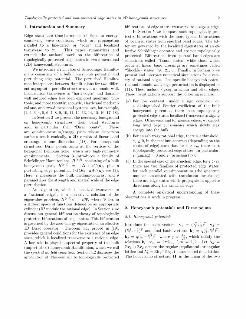
interpenetrating triangular lattices: A+Λh and B+Λh,where A = (0, 0)T and B = ( 1√

3, 0)T ; see Figure

1(a). Bh denotes the Brillouin zone, the choice offundamental cell in quasi-momentum space is displayedin Figure 1(b).

A honeycomb lattice potential, V (x), is a real-valued, smooth function, which is Λh− periodic and,relative to some origin of coordinates, is inversionsymmetric (even) and invariant under a 2π/3 rotation.Specifically, if R denotes the 2 × 2 rotation matrix by2π/3, we have R[V ](x) ≡ V (R∗x) = V (x). A naturalchoice of period cell is Ωh, the parallelogram in R2

spanned by v1,v2.Consider the Hamiltonian for the unperturbed

honeycomb structure:

H(ε,0) = −∆ + εV (x). (1)

The band structure of the Λh− periodic Schrodingeroperator, H(ε,0), is obtained from the family ofeigenvalue problems, parametrized by k ∈ Bh:(H(ε,0) − E)Ψ = 0, Ψ(x + v) = eik·vΨ(x), x ∈R2, v ∈ Λh. We denote by L2

k the space of functionsf ∈ L2

loc satisfying the k− pseudo-periodic boundarycondition f(x + v) = eik·vf(x). For f and g in L2

k,fg is in L2(R2/Λ) and we define their inner productby 〈f, g〉L2

k=∫

Ωf(x)g(x)dx. Equivalently, ψ(x) =

e−ik·xΨ(x) satisfies the periodic eigenvalue problem:(H(ε,0)(k)− E(k)

)ψ = 0 and ψ(x + v) = ψ(x) for all

x ∈ R2 and v ∈ Λh, where

H(ε,0)(k) = −(∇+ ik)2 + εV (x).

For each k ∈ Bh, the spectrum is real and consistsof discrete eigenvalues Eb(k), b ≥ 1, where Eb(k) ≤Eb+1(k). The graphs of k 7→ Eb(k) ∈ R arecalled the dispersion surfaces of H(ε,0). The collectionof these surfaces constitutes the band structure ofH(ε,0). As k varies over Bh, each map k → Eb(k) isLipschitz continuous and sweeps out a closed intervalin R. The union of these intervals is the L2(R2)−spectrum of H(ε,0). More detail on the generaltheory of periodic operators and the specific contextof honeycomb structures appears in [22, 23, 24] and[25, 19], respectively.

2.2. Dirac points

Let V denote a honeycomb lattice potential. Diracpoints of H(ε,0) are quasimomentum/energy pairs,(K?, E?), in the band structure of H(ε,0) at whichneighboring dispersion surfaces touch conically at apoint [26, 27, 25]. In particular, there exists a b? ≥ 1such that:

(i) E? = Eb?(K?) = Eb?+1(K?) is a two-folddegenerate L2

K?− eigenvalue of H(ε,0).

Figure 1. (a): A = (0, 0), B = ( 1√3, 0). The honeycomb

structure, H, is the union of two sub-lattices ΛA = A+Λh (blue)and ΛB = B + Λh (red). The lattice vectors v1,v2 generateΛh. (b): Brillouin zone, Bh, and dual basis k1,k2. K and K′

are labeled. (c): Zigzag edge (solid line), Rv1 = x : k2 ·x = 0,armchair edge (dashed line), R (v1 + v2) = x : (k1 − k2) · x =0, and a fundamental domain for the cylinder for the zigzagedge (gray area), ΣZZ. (d): Schematic of edge state, localizedtransverse to the zigzag edge (Rv1).

(ii) Nullspace(H(ε,0) − E?I) = spanΦ1(x),Φ2(x),where Φ1 ∈ L2

K?,τ= L2

K?∩ f : Rf = τf and

Φ2(x) = Φ1(−x) ∈ L2K?,τ

= L2K?∩f : Rf = τf,

and 〈Φa,Φb〉L2K?

(Ω) = δab, a, b = 1, 2. Here,

τ = exp(2πi/3). We note that 1, τ and τ areeigenvalues of the rotation matrix, R.

(iii) There exist L2k− Floquet-Bloch eigenpairs k 7→

(Φb?(x; k), Eb?(k)) and k 7→ (Φb?+1(x; k), Eb?+1(k)),defined in a neighborhood of K?, such that

Eb?+1(k)− E? ≈ +|λ]| |k−K?| ,Eb?(k)− E? ≈ −|λ]| |k−K?| .where |λ]| = 2| 〈Φ2, ζ · ∇Φ1〉L2

K?

| 6= 0 for any

ζ = (ζ1, ζ2) ∈ C2, such that ‖ζ‖C2 = 1.

In [25] (see also [28], Appendix D), Fefferman andWeinstein proved the following:

Theorem 2.1 (a) For all ε real outside a possiblediscrete set, the Hamiltonian H(ε,0) = −∆ + εV hasDirac points occurring at (K?, E?), where K? maybe any of the six vertices of the Brillouin zone, Bh.(b) If 0 < |ε| < ε0 is sufficiently small, then thereare two cases, which are delineated by the sign ofthe distinguished Fourier coefficient, εV1,1, of εV (x).Here,

V1,1 ≡1

|Ωh|

∫Ωh

e−i(k1+k2)·yV (y)dy, (2)

is assumed to be non-zero. If εV1,1 > 0, then b? = 1;Dirac points occur at the intersection of the first and

Topologically protected and non-protected edge states in 2D honeycomb structures 4

4

2

0

k(1)

-2

-4-4-2

k(2)

02

4

30

20

10

0

40

E

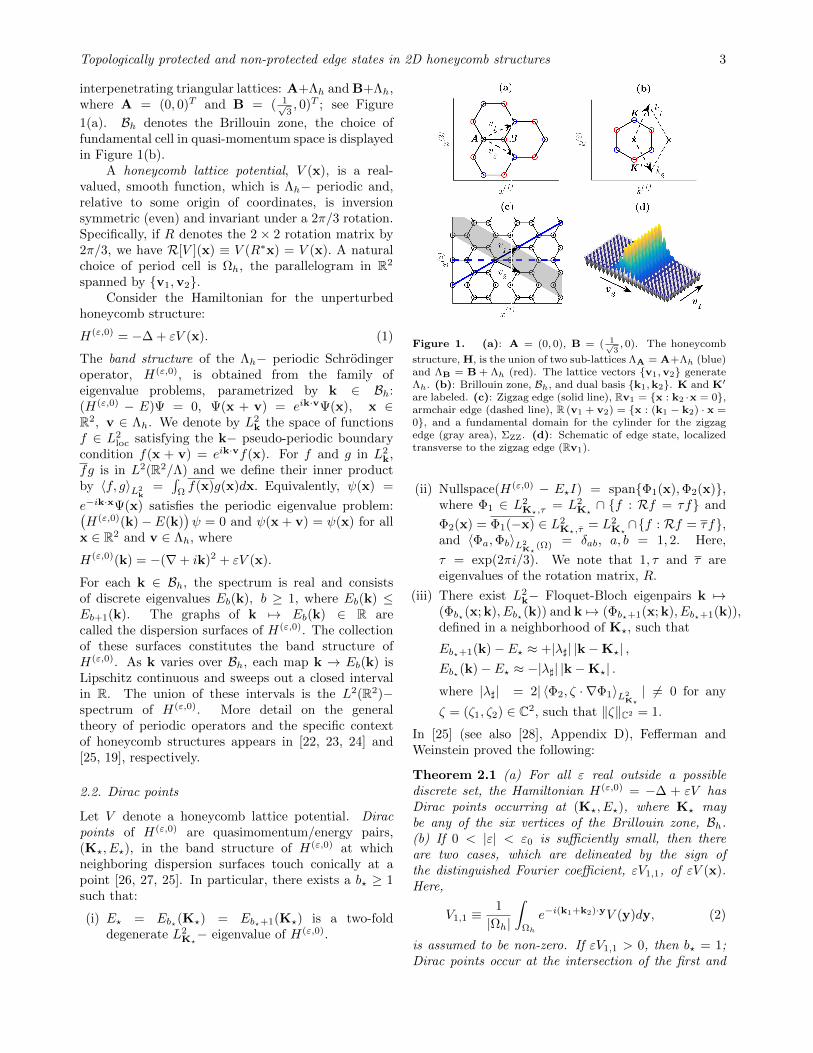
Figure 2. Lowest three dispersion surfaces k ≡(k(1), k(2)) ∈ Bh 7→ E(k) of the band structure of H(10,0) ≡−∆ + 10V (x), where V is a honeycomb potential: V (x) =(cos(k1 · x) + cos(k2 · x) + cos((k1 + k2) · x)). Dirac pointsoccur at the conical intersection of the lower two dispersionsurfaces, at the six vertices of the Brillouin zone, Bh.

second dispersion surfaces (see Figure 2). If εV1,1 < 0,then b? = 2; they occur at the intersection of the secondand third dispersion surfaces.

The two cases in part (b) of Theorem 2.1 are illustratedin Figure 3 (top row, left and center plots).

The quasimomenta of Dirac points partitioninto two equivalence classes; the K− points (K =13 (k1 − k2)) consisting of K, RK and R2K, and K′−points (K′ = −K) consisting of K′ = −K, RK′ andR2K′; see Figure 1(b). By symmetries, the localcharacter near one Dirac point determines the localcharacter near the others.

The time evolution of a wave packet, with dataspectrally localized near a Dirac point, is governed bya massless 2D Dirac system [29].

Remark 2.1 It is shown in [25] that a Λh− periodicperturbation of V (x), which breaks inversion or time-reversal symmetry, lifts the eigenvalue degeneracy;a (local) gap is opened about the Dirac points andthe perturbed dispersion surfaces are locally smooth.The edge potential we introduce opens such a gap, asillustrated in the bottom row of Figure 3.

3. Honeycomb structure with an edge and theedge state eigenvalue problem

We follow the setup introduced in [19]. Recall (Section2.1) the spanning vectors of the equilateral triangularlattice, v1 and v2. Given a pair of integers a1, b1,which are relatively prime, let v1 = a1v1 + b1v2.We call the line Rv1 the v1− edge. Since a1, b1 are

relatively prime, there exists a second pair of relativelyprime integers: a2, b2 such that a1b2 − a2b1 = 1. Setv2 = a2v1 + b2v2.

It follows that Zv1⊕Zv2 = Zv1⊕Zv2 = Λh. Sincea1b2 − a2b1 = 1, we have dual lattice vectors K1,K2 ∈Λ∗h, given by K1 = b2k1−a2k2 and K2 = −b1k1+a1k2,which satisfy K` · v`′ = 2πδ`,`′ , 1 ≤ `, `′ ≤ 2. Notethat ZK1 ⊕ ZK2 = Zk1 ⊕ Zk2 = Λ∗h. We denote byΩ the period cell given by the parallelogram spannedby v1,v2. The choice v1 = v1 (or equivalently v2)generates a zigzag edge and the choice v1 = v1 + v2

generates the armchair edge; see Figure 1(c).Introduce the family of Hamiltonians, depending

on the real parameters ε and δ:

H(ε,δ) ≡ −∆ + εV (x) + δκ(δK2 · x)W (x). (3)

H(ε,0) = −∆ + εV (x) is the Hamiltonian for theunperturbed (bulk) honeycomb structure, introducedin (1) and discussed in Theorem 2.1. Here, δ willbe taken to be sufficiently small, and W (x) is Λh−periodic and odd. The function κ(ζ) defines a domainwall. We choose κ to be sufficiently smooth and tosatisfy κ(0) = 0 and κ(ζ) → ±κ∞ 6= 0 as ζ → ±∞,e.g. κ(ζ) = tanh(ζ). Without loss of generality, weassume κ∞ > 0.

Note that H(ε,δ) is invariant under translationsparallel to the v1− edge, x 7→ x+v1, and hence there isa well-defined parallel quasimomentum (good quantumnumber), denoted k‖. Furthermore, H(ε,δ) transitionsadiabatically between the asymptotic Hamiltonian

H(ε,δ)− = H(ε,0) − δκ∞W (x) as K2 · x → −∞ to the

asymptotic Hamiltonian H(ε,δ)+ = H(ε,0) + δκ∞W (x)

as K2 · x → ∞. The domain wall modulation ofW (x) realizes a phase-defect across the edge Rv1.A variant of this construction was used in [12, 28]to interpolate between different asymptotic 1D dimerperiodic potentials.

We seek v1− edge states of H(ε,δ), which arespectrally localized near the Dirac point, (K?, E?).These are non-trivial solutions Ψ, with energies E ≈E?, of the k‖− edge state eigenvalue problem (EVP):

H(ε,δ)Ψ = EΨ, (4)

Ψ(x + v1) = eik‖Ψ(x), (5)

|Ψ(x)| → 0 as |K2 · x| → ∞, (6)

for k‖ ≈ K? · v1. The boundary conditions (5) and(6) imply, respectively, propagation parallel to, andlocalization transverse to, the edge Rv1.

We next formulate the edge state eigenvalueproblem (4)-(6) in an appropriate Hilbert space.Introduce the cylinder Σ ≡ R2/Zv1. Denote byHs(Σ), s ≥ 0, the Sobolev spaces of functions definedon Σ. The pseudo-periodicity and decay conditions(5)-(6) are encoded by requiring Ψ ∈ Hs

k‖(Σ) = Hs

k‖,

Topologically protected and non-protected edge states in 2D honeycomb structures 5

for some s ≥ 0, where

Hsk‖≡f : f(x)e−i

k‖2πK1·x ∈ Hs(Σ)

.

We then formulate the EVP (4)-(6) as:

H(ε,δ)Ψ = EΨ, Ψ ∈ H2k‖

(Σ). (7)

3.1. The spectral no-fold condition

Now suppose H(ε,0) has a Dirac point at (K?, E?),i.e. ε is generic (not necessarily small) in the senseof Theorem 2.1. (Recall, from Section 2 that all vertexquasimomenta of the hexagon, Bh, have Dirac pointswith energy E?.) While H(ε,0) is inversion symmetric

(invariant under x 7→ −x), H(ε,δ)± is not. Therefore,

by Remark 2.1, for δ 6= 0, H(ε,δ)± does not have Dirac

points; its dispersion surfaces are locally smooth andfor quasimomenta k such that |k −K?| is sufficientlysmall, there is an open neighborhood of E = E? not

contained in the L2(R2/Λh)− spectrum of H(ε,δ)± (k).

If there is a (real) open neighborhood of E = E?, not

contained in the spectrum of H(ε,δ)± (k) for all k ∈ Bh,

then H(ε,δ)± is said to have a (global) omni-directional

spectral gap about E = E?. But, the “spectral gap”about E = E?, created for δ 6= 0 and small, mayonly be local about K?. What is central howeverto the existence of v1− edge states is that along thedispersion surface slice, dual to the v1− edge, H(ε,0)

satisfy a spectral no-fold condition. We now explainthis condition, without going into all technical detail.

Let (K?, E?) denote a Dirac point of H(ε,0) inthe sense of Section 2.1, where E? = Eb?(K?) =Eb?+1(K?). Consider the dual slice associated withthe v1− edge, i.e. the union of graphs of the functionsλ ∈ (−1/2, 1/2] 7→ Eb(K? + λK2), b ≥ 1. Thevalues swept out constitute the L2

k‖=K?·v1− spectrum.

Within this slice, the graphs of λ 7→ Eb?(K? + λK2)and λ 7→ Eb?+1(K? +λK2) may intersect at either oneor two independent Dirac points, i.e. points in thelattices K + Λ∗h or in K′ + Λ∗h, occurring at distinctvalues of λ ∈ (−1/2, 1/2]. (E.g. for a zigzag edge

there is one value, namely λ1 = 0, and for an armchairedge there are two, namely λ1 = 0 and λ2 = −1/3.)The preceding discussion implies that a L2

k‖=K?·v1−

spectral gap of H(ε,δ)± is opened locally near each Dirac

point, i.e. for all λ near λj , by the domain wall/edgepotential for δ 6= 0 and small; see Figure 3.

We say that the spectral no-fold condition issatisfied for the v1− edge if, for δ 6= 0, the L2

k‖=K?·v1−

spectrum of H(ε,δ)± has a full spectral gap. That is, the

L2k‖=K?·v1

− spectrum of H(ε,δ)± does not intersect some

open interval containing E?.

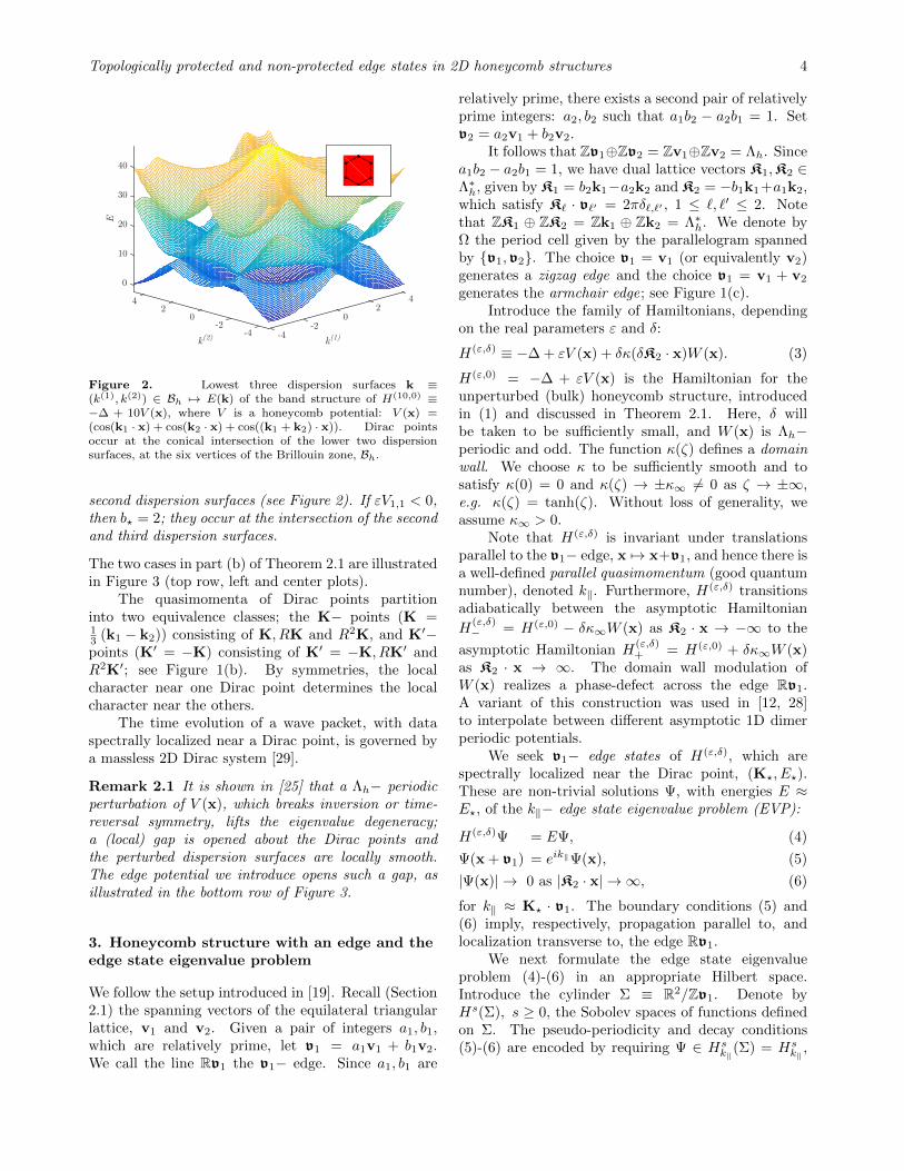
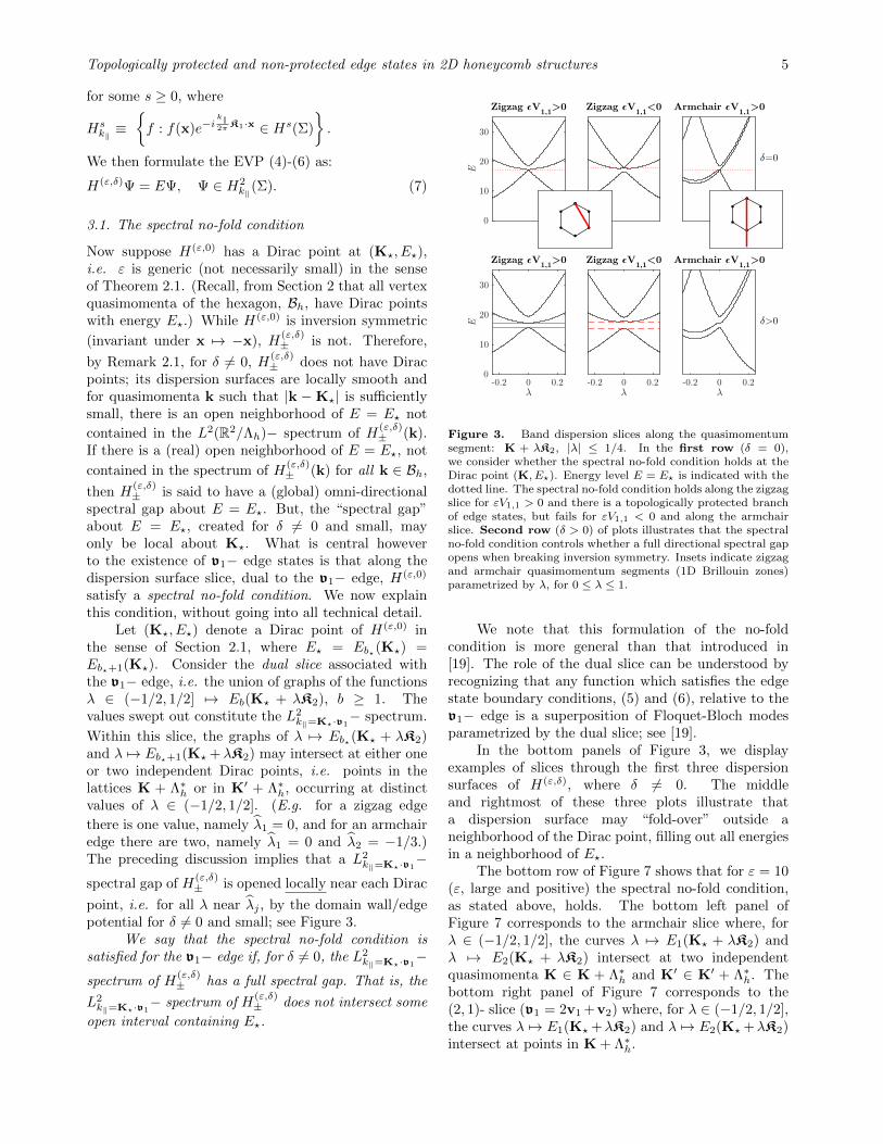
Figure 3. Band dispersion slices along the quasimomentumsegment: K + λK2, |λ| ≤ 1/4. In the first row (δ = 0),we consider whether the spectral no-fold condition holds at theDirac point (K, E?). Energy level E = E? is indicated with thedotted line. The spectral no-fold condition holds along the zigzagslice for εV1,1 > 0 and there is a topologically protected branchof edge states, but fails for εV1,1 < 0 and along the armchairslice. Second row (δ > 0) of plots illustrates that the spectralno-fold condition controls whether a full directional spectral gapopens when breaking inversion symmetry. Insets indicate zigzagand armchair quasimomentum segments (1D Brillouin zones)parametrized by λ, for 0 ≤ λ ≤ 1.

We note that this formulation of the no-foldcondition is more general than that introduced in[19]. The role of the dual slice can be understood byrecognizing that any function which satisfies the edgestate boundary conditions, (5) and (6), relative to thev1− edge is a superposition of Floquet-Bloch modesparametrized by the dual slice; see [19].

In the bottom panels of Figure 3, we displayexamples of slices through the first three dispersionsurfaces of H(ε,δ), where δ 6= 0. The middleand rightmost of these three plots illustrate thata dispersion surface may “fold-over” outside aneighborhood of the Dirac point, filling out all energiesin a neighborhood of E?.

The bottom row of Figure 7 shows that for ε = 10(ε, large and positive) the spectral no-fold condition,as stated above, holds. The bottom left panel ofFigure 7 corresponds to the armchair slice where, forλ ∈ (−1/2, 1/2], the curves λ 7→ E1(K? + λK2) andλ 7→ E2(K? + λK2) intersect at two independentquasimomenta K ∈ K + Λ∗h and K′ ∈ K′ + Λ∗h. Thebottom right panel of Figure 7 corresponds to the(2, 1)- slice (v1 = 2v1 +v2) where, for λ ∈ (−1/2, 1/2],the curves λ 7→ E1(K? +λK2) and λ 7→ E2(K? +λK2)intersect at points in K + Λ∗h.

Topologically protected and non-protected edge states in 2D honeycomb structures 6

4. Topologically protected edge states

4.1. General conditions for topologically protectedbifurcations of edge states for rational edges

In this section we review conditions on the Hamilto-nian, H(ε,δ), defined in (3), guaranteeing the existenceof topologically protected states for an arbitrary v1−edge. These results are proved in [19] (Theorem 7.3and Corollary 7.4).

Let V be a honeycomb lattice potential (seeSection 2.1) and W be real-valued, Λh− periodic andodd. Assume that H(ε,0) = −∆ + εV has a Diracpoint (K?, E?), where K? is a vertex of Bh as definedin Section 2.2. Assume further that H(ε,0) satisfies thespectral no-fold condition for the v1− edge, as statedin [28]. That is, we assume that the quasi-momentumslice through only intersects one independent Diracpoint; see the discussion of Section 3.1. ‡ Finally,we assume the non-degeneracy condition:

ϑ] ≡ 〈Φ1,WΦ1〉L2K?

6= 0, (8)

where Φ1(x) is the L2K?− eigenfunction of H(ε,0)

associated with the quasimomentum K? introduced inSection 2.2.

Theorem 4.1 Under the above hypotheses:

(i) There exist topologically protected v1− edge stateswith k‖ = K? · v1, constructed as a bifurcation

curve of non-trivial eigenpairs δ 7→ (Ψδ, Eδ) of(7), defined for all |δ| sufficiently small. Thisbranch of non-trivial states bifurcates from thetrivial solution branch E 7→ (Ψ ≡ 0, E) at E =E?. The edge state, Ψδ(x), is well-approximated(in H2

k‖=K·v1) by a slowly varying and spatially

decaying modulation of the degenerate nullspace ofH(ε,0) − E?:

Ψδ(x) ≈ α?,+(δK2 · x)Φ+(x) + α?,−(δK2 · x)Φ−(x),

Eδ = E? +O(δ2), 0 < |δ| 1,

where Φ+ and Φ− are appropriate linear combi-nations of Φ1 and Φ2. The envelope amplitude-vector, α?(ζ) = (α?,+(ζ), α?,−(ζ))T , is a zero-energy eigenstate, Dα? = 0, of the 1D Dirac op-erator:

D ≡ −i|λ]||K2|σ3∂ζ + ϑ]κ(ζ)σ1 . (9)

Here, σ1 and σ3 are standard Pauli matrices.

(ii) Topological protection: The Dirac operator D hasa spatially localized zero-energy eigenstate for anyκ(ζ) having asymptotic limits of opposite signat ±∞. Therefore, the zero-energy eigenstate,which seeds the bifurcation, persists for localized

‡ An article in which we extend this theorem to the situationwhere both classes of Dirac points lie in the dual slice is inpreparation.

perturbations of κ(ζ). In this sense, the bifurcatingbranch of edge states is topologically protectedagainst a class of local (not necessarily small)perturbations of the edge.

(iii) Edge states, Ψ(x; k‖) ∈ H2k‖

, exist for all

parallel quasimomenta k‖ in a neighborhood ofk‖ = K · v1, and by symmetry for all k‖ in aneighborhood of k‖ = −K · v1 = K′ · v1. Itfollows that by taking a continuous superpositionof the time-harmonic states, Ψ(x, k‖)e

−iE(k‖)t,one obtains wave-packets that remain localizedabout (and dispersing along) the v1− edge for alltime.

We next apply Theorem 4.1 to the study of edge stateswhich are localized transverse to a zigzag edge.

4.2. Topologically protected zigzag edge states

The zigzag edge corresponds to the choice: v1 = v1,v2 = v2, and K1 = k1, K2 = k2. In Section 8 of [19]we apply our general Theorem 4.1 to study the zigzagedge eigenvalue problem H(ε,δ)Ψ = EΨ, Ψ ∈ H2

k‖(Σ),

where Σ = R2/Zv1, for the Hamiltonian (3) with:

0 < |δ| . ε2 1. (10)

There are two cases, which are delineated by the sign ofthe distinguished Fourier coefficient of the unperturbed(bulk) honeycomb potential:

(1) εV1,1 > 0 and (2) εV1,1 < 0,

where V1,1, defined in (2), is assumed to be non-zero.For appropriate choices of V (x), it is possible to tunebeen cases (1) and (2) by varying of the lattice scaleparameter; see Appendix A of [19].

Remark 4.1 The computer simulations discussed inthis and subsequent sections were done for theHamiltonian H(ε,δ) with κ(ζ) = tanh(ζ) and

V (x) =∑

kj∈k1,k2,k1+k2

cos(kj · x),

W (x) =∑

kj∈k1,k2,k1+k2

sin(kj · x).(11)

Here, k1 and k2 are displayed in Section 2.1. SinceV1,1 > 0, sgn(εV1,1) is determined by the sign of ε.

Case (1) εV1,1 > 0 and (10): In this case, thespectral no-fold condition holds for the zigzag edge(Theorem 8.2 of [19]) and it follows that there existzigzag edge states (Theorem 8.5 of [19]). In particular,for all ε and δ satisfying (10), the zigzag edge stateeigenvalue problem (7) has topologically protectededge states, described in Theorem 4.1, with L2

k‖−

spectra of energies: k‖ 7→ E(k‖) (k‖ varying nearK · v1 = 2π/3 and varying near −K · v1 = −2π/3)sweeping out a neighborhood of E = E?.

Topologically protected and non-protected edge states in 2D honeycomb structures 7

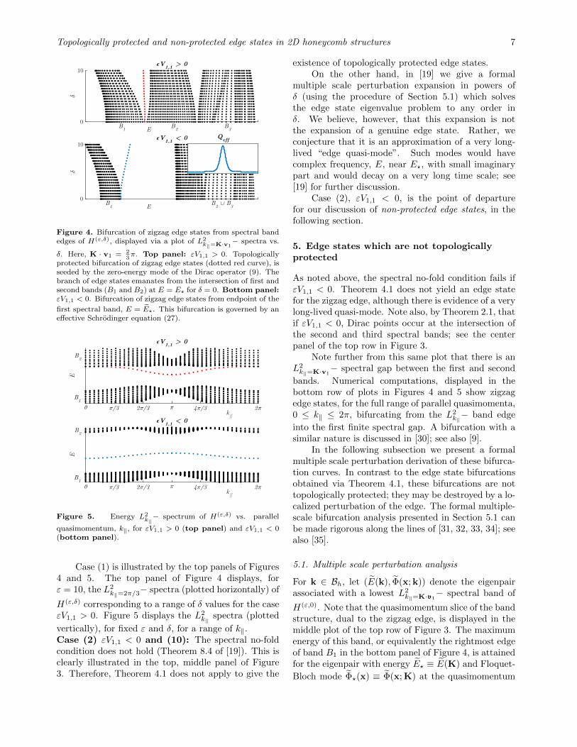
Figure 4. Bifurcation of zigzag edge states from spectral bandedges of H(ε,δ), displayed via a plot of L2

k‖=K·v1− spectra vs.

δ. Here, K · v1 = 23π. Top panel: εV1,1 > 0. Topologically

protected bifurcation of zigzag edge states (dotted red curve), isseeded by the zero-energy mode of the Dirac operator (9). Thebranch of edge states emanates from the intersection of first andsecond bands (B1 and B2) at E = E? for δ = 0. Bottom panel:εV1,1 < 0. Bifurcation of zigzag edge states from endpoint of the

first spectral band, E = E?. This bifurcation is governed by aneffective Schrodinger equation (27).

Figure 5. Energy L2k‖− spectrum of H(ε,δ) vs. parallel

quasimomentum, k‖, for εV1,1 > 0 (top panel) and εV1,1 < 0(bottom panel).

Case (1) is illustrated by the top panels of Figures4 and 5. The top panel of Figure 4 displays, forε = 10, the L2

k‖=2π/3− spectra (plotted horizontally) of

H(ε,δ) corresponding to a range of δ values for the caseεV1,1 > 0. Figure 5 displays the L2

k‖spectra (plotted

vertically), for fixed ε and δ, for a range of k‖.Case (2) εV1,1 < 0 and (10): The spectral no-foldcondition does not hold (Theorem 8.4 of [19]). This isclearly illustrated in the top, middle panel of Figure3. Therefore, Theorem 4.1 does not apply to give the

existence of topologically protected edge states.On the other hand, in [19] we give a formal

multiple scale perturbation expansion in powers ofδ (using the procedure of Section 5.1) which solvesthe edge state eigenvalue problem to any order inδ. We believe, however, that this expansion is notthe expansion of a genuine edge state. Rather, weconjecture that it is an approximation of a very long-lived “edge quasi-mode”. Such modes would havecomplex frequency, E, near E?, with small imaginarypart and would decay on a very long time scale; see[19] for further discussion.

Case (2), εV1,1 < 0, is the point of departurefor our discussion of non-protected edge states, in thefollowing section.

5. Edge states which are not topologicallyprotected

As noted above, the spectral no-fold condition fails ifεV1,1 < 0. Theorem 4.1 does not yield an edge statefor the zigzag edge, although there is evidence of a verylong-lived quasi-mode. Note also, by Theorem 2.1, thatif εV1,1 < 0, Dirac points occur at the intersection ofthe second and third spectral bands; see the centerpanel of the top row in Figure 3.

Note further from this same plot that there is anL2k‖=K·v1

− spectral gap between the first and second

bands. Numerical computations, displayed in thebottom row of plots in Figures 4 and 5 show zigzagedge states, for the full range of parallel quasimomenta,0 ≤ k‖ ≤ 2π, bifurcating from the L2

k‖− band edge

into the first finite spectral gap. A bifurcation with asimilar nature is discussed in [30]; see also [9].

In the following subsection we present a formalmultiple scale perturbation derivation of these bifurca-tion curves. In contrast to the edge state bifurcationsobtained via Theorem 4.1, these bifurcations are nottopologically protected; they may be destroyed by a lo-calized perturbation of the edge. The formal multiple-scale bifurcation analysis presented in Section 5.1 canbe made rigorous along the lines of [31, 32, 33, 34]; seealso [35].

5.1. Multiple scale perturbation analysis

For k ∈ Bh, let (E(k), Φ(x; k)) denote the eigenpairassociated with a lowest L2

k‖=K·v1− spectral band of

H(ε,0). Note that the quasimomentum slice of the bandstructure, dual to the zigzag edge, is displayed in themiddle plot of the top row of Figure 3. The maximumenergy of this band, or equivalently the rightmost edgeof band B1 in the bottom panel of Figure 4, is attainedfor the eigenpair with energy E? ≡ E(K) and Floquet-

Bloch mode Φ?(x) ≡ Φ(x; K) at the quasimomentum

Topologically protected and non-protected edge states in 2D honeycomb structures 8

k = K. More generally, we may consider any vertexquasimomenta, K?, such that the L2

K?− nullspace of

H(ε,δ) − E?I has dimension one, which is the case inthe numerical examples we have considered.

We keep the discussion general and consider ageneral v1− edge (recall the setup at the beginningof Section 3) and seek a solution of the v1− edge stateeigenvalue problem (4)-(6) (see also (7)) of the multi-scale form: Ψ = Ψ(x, ζ) with ζ = δK2 · x. In terms ofthese variables:[− (∇x + δK2∂ζ)

2+ εV (x) + δκ(ζ)W (x)

]Ψ(x; ζ)

= E Ψ(x; ζ)

Ψ(x + v1, ζ) = eiK?·v1Ψ(x, ζ),

ζ 7→ Ψ(x, ζ) ∈ L2(Rζ).

(12)

We seek a solution to (12) via a multiple scaleexpansion in δ, assumed to be small:

Eδ = E(0) + δE(1) + δ2E(2) + . . . ,

Ψδ = Ψ(0)(x, ζ) + δΨ(1)(x, ζ) + δ2Ψ(2)(x, ζ) + . . . .(13)

The boundary conditions (5) and (6) are imposed byrequiring, for i ≥ 0:

Ψ(i)(x + v1, ·) = eiK?·v1Ψ(i)(x, ·),ζ → Ψ(i)(x, ζ) ∈ L2(Rζ).

Substituting (13) into (12) and equating terms ofequal order in δi, i ≥ 0, yields a hierarchy ofnon-homogeneous boundary value problems, governingΨ(i)(x, ζ). Each equation in this hierarchy is viewedas a PDE with respect to x, with pseudo-periodicboundary conditions. The solvability conditionsfor this hierarchy determine the ζ− dependence ofΨδ(x, ζ).

At order δ0 we have that (E(0),Ψ(0)) satisfy(−∆x + εV (x)− E(0)

)Ψ(0) = 0,

Ψ(0)(x + v, ζ) = eiK?·vΨ(0)(x, ζ), for all v ∈ Λh.(14)

Equation (14) has solution

E(0) = E?, Ψ(0)(x, ζ) = A0(ζ)Φ?(x), (15)

where, Φ? (normalized in L2(Ω)) spans the nullspace

of H(ε,0) − E?I.Proceeding to order δ1 we find that (Ψ(1), E(1))

satisfies

(−∆x + εV (x)− E?) Ψ(1)(x, ζ) = G(1)(x, ζ)

Ψ(1)(x + v, ζ) = eiK?·vΨ(1)(x, ζ), for all v ∈ Λh,(16)

where

G(1)(x, ζ) = G(1)(x, ζ; Ψ(0), E(1))

≡ 2∂ζA0(ζ) K2 · ∇xΦ?(x)

+(−κ(ζ)W (x) + E(1)

)A0(ζ)Φ?(x).

(17)

A necessary condition for the solvability of (16) is thatthe inhomogeneous term on the right hand side beL2K?

(Ω; dx)− orthogonal to Φ?(x). By the symmetries

Φ?(x) = Φ?(−x) and W (x) = −W (−x),⟨Φ?,W Φ?

⟩L2

K?(Ω)

= 0,⟨

Φ?,∇Φ?

⟩L2

K?(Ω)

= 0. (18)

Therefore, with E(1) ≡ 0, the right hand side of (16)

lies in the range of H(ε,0)− E?I : H2K?→ L2

K?, and we

obtain

Ψ(1)(x, ζ) =(R(E?)G

(1))

(x, ζ; 0), (19)

where R(E?) = (H(ε,0)− E?I)−1 : P⊥L2(Ω)→ H2(Ω).

Here, P⊥ is the L2− projection onto spanΦ?⊥.At order δ2, we have(

−∆x + εV (x)− E?)

Ψ(2)(x, ζ) = G(2)(x, ζ)

Ψ(2)(x + v, ζ) = eiK?·vΨ(2)(x, ζ), for all v ∈ Λh,(20)

where

G(2)(x, ζ) = G(2)(x, ζ; Ψ(0),Ψ(1), E(2))

≡ (2∇x ·K2∂ζ − κ(ζ)W (x))ψ(1)p

+ |K2|2∂2ζA0(ζ)Φ?(x) + E(2)A0(ζ)Φ?(x).

Equation (20) has a solution if and only if the right

hand side is L2K?

-orthogonal to Φ?. This solvabilitycondition (all inner products over L2

K?(Ωx)) is:

|K2|2∂2ζA0(ζ) +

⟨Φ?(x), 2∇x ·K2∂ζΨ

(1)(x, ζ)⟩

(21)

−⟨

Φ?(x), κ(ζ)WΨ(1)(x, ζ)⟩

+ E(2)A0(x) = 0.

We simplify (21) using the expression for Ψ(1) in(19); see also (17). Importantly, note that the action

of the resolvent R(E?) on the individual terms in (17)is well defined due to (18). After some manipulation,the first inner product in (21) yields⟨

Φ?(x), 2∇x ·K2∂ζΨ(1)(x, ζ)

⟩= −4

∑1≤i,j≤2

⟨∂xiΦ?(x), R(E?)(∂xj Φ?)

⟩K

(i)2 K

(j)2 ∂2

ζA0(ζ)

+ 2⟨∇xΦ?, R(E?)(W Φ?)

⟩·K2∂ζ(κ(ζ)A0(ζ)), (22)

while the second inner product in (21) yields

−⟨

Φ?(x), κ(ζ)W (x)Ψ(1)(x, ζ)⟩

= −2⟨

Φ?,WR(E?)(∇xΦ?)⟩·K2κ(ζ)∂ζA0(ζ)

+⟨

Φ?,WR(E?)(W Φ?)⟩κ2(ζ)A0(ζ). (23)

It can be checked that⟨Φ?,WR(E?)(W Φ?)

⟩L2

K?(Ω)

> 0 and that (24)⟨Φ?,WR(E?)(∇xΦ?)

⟩L2

K?(Ωx)

is real. (25)

Topologically protected and non-protected edge states in 2D honeycomb structures 9

Relation (24) follows since E? is the lowest eigenvalueof H(ε,0)(K?). Moreover we have that

δij |K2|2 − 4∑

1≤i,j≤2

⟨∂xiΦ?(x), R(E?)(∂xj Φ?)

⟩K

(i)2 K

(j)2

=1

2[D2E?(K?)]ijK

(i)2 K

(j)2 ≡ 1

2meff, (26)

where D2E?(K?) is the Hessian matrix of E(k)evaluated at k = K? along the K2− quasimomentumdirection, and meff is the effective mass [36]; see alsoTheorem 3.1 and equation (3.6) of [31].

Substituting (22) and (23) into equation (21), andusing relations (25) and (26), we find that the O(δ2)solvability condition reduces to the eigenvalue problemfor an effective Schrodinger operator, Heff :

HeffA0(ζ) = µeffA0(ζ), A0(ζ) ∈ L2(Rζ), where

Heff ≡ −1

2meff∂2ζ +Qeff(ζ;κ),

(27)

with eigenvalue parameter µeff = E(2) + b κ2∞ and

effective potential, Qeff , given by:

Qeff(ζ;κ)

= −2⟨K2 · ∇xΦ?, R(E?)(W Φ?)

⟩L2

K?(Ω)

κ′(ζ)

+⟨W Φ?, R(E?)(W Φ?)

⟩L2

K?(Ω)

(κ2∞ − κ2(ζ)

)≡ a κ′(ζ) + b

(κ2∞ − κ2(ζ)

). (28)

The constants a and b depend on Φ?, V and W and,by (24), b > 0. Since κ(ζ) satisfies κ(ζ) → ±κ∞ asζ → ±∞, both κ′(ζ) and κ2

∞ − κ2(ζ) decay to zero asζ → ±∞. Therefore, Qeff(ζ;κ) is decaying at infinity.

If the eigenvalue problem (27) has a non-trivialsolution, then the above formal expansion yields asolution of the v1− edge state eigenvalue problem toarbitrary finite order in δ. This formal expansion yieldsapproximations to arbitrary finite order of genuinesolutions of the v1− edge state eigenvalue problem,δ 7→ (Ψδ(x), Eδ).

In summary, the non-trivial eigensolutions of theeffective Schrodinger operator, Heff , seed or inducethe bifurcation of non-trivial edge states in a manneranalogous to the zero-energy eigenmodes of a Diracoperator inducing the bifurcation of protected edgestates from Dirac points. In the next section weshow that such “effective Schrodinger bifurcations”,also known as “Tamm states”, are not topologicallyprotected; these states do not persist in the presenceof arbitrary localized perturbations of the domain wall.

5.2. Edge states seeded by localized eigenstates of theeffective Schrodinger operator, Heff , are nottopologically protected

We now explore the robustness of the edge statebifurcating from the trivial state E = E? for δ = 0,

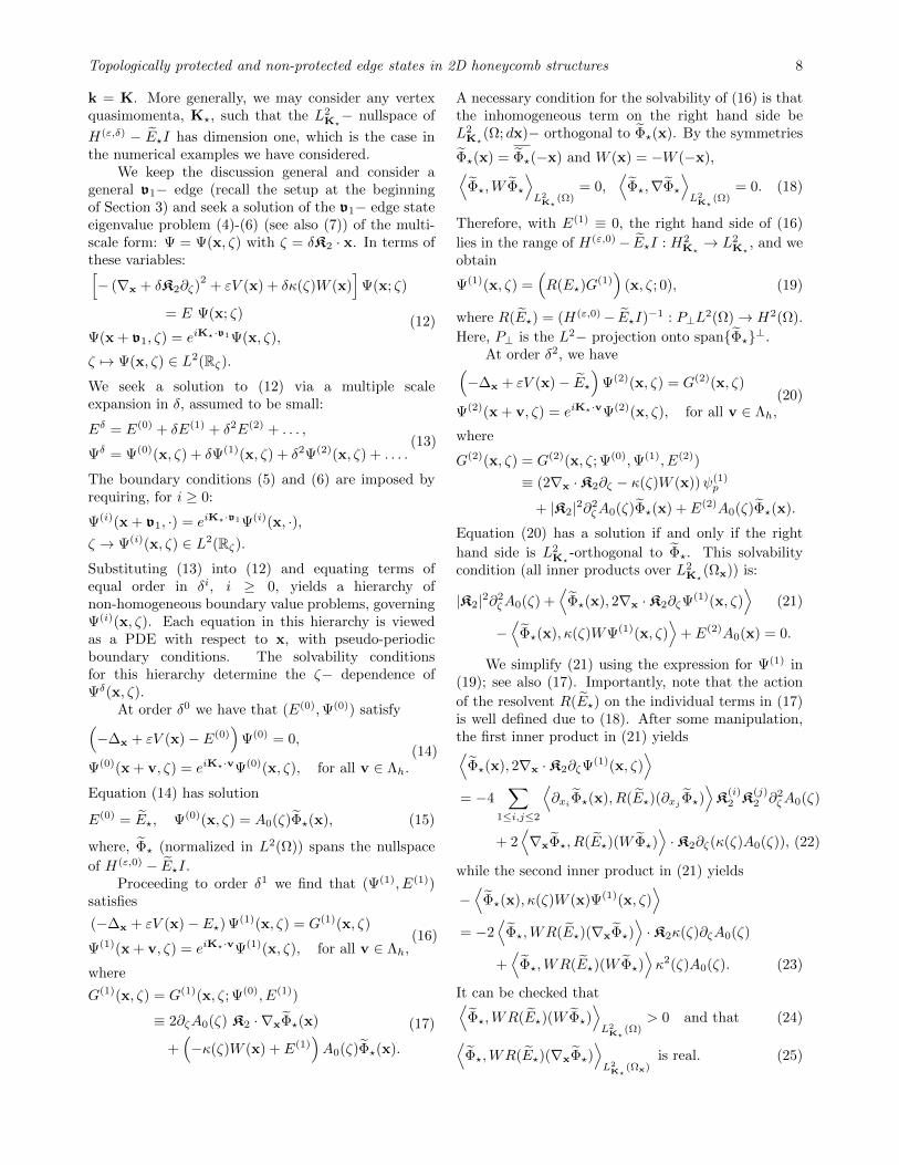
Figure 6. Bifurcation curves of non-protected edge statesfrom spectral band edges, encoded in L2

k‖=2π/3− spectra vs.

δ for the Hamiltonian H(−10,δ) for εV1,1 < 0. Top panel:κ(ζ) = tanh(ζ). Bottom panel: κ\(ζ) = κ(ζ) + F (ζ) =tanh(ζ)+10 exp(−ζ2/50). The branch of edge states bifurcating

from the top edge of the lowest band, B1, at E = E? for δ = 0(blue dotted curve in top panel) is destroyed by the perturbationF (ζ). Insets show the effective potential Qeff in each case.

constructed in Section 5.1. We focus on the case ofthe zigzag edge, corresponding to the choice v1 = v1,v2 = v2 and K1 = k1, K2 = k2. We also fix V , Wand κ(ζ) = tanh(ζ) as in (11), with ε = −10 so thatεV1,1 < 0. From numerics we havem−1

eff < 0 (this is alsoclear from the top, center panel of Figure 3 and Figure6). Moreover, a > 0 and, as argued above, b > 0.Therefore, κ′(ζ) = sech2(ζ) and κ2

∞−κ2(ζ) = sech2(ζ)are non-negative and it follows that Qeff(ζ;κ) (28),plotted in the inset of Figure 4 (and the top insetof Figure 6), is a potential barrier. Therefore, sincem−1

eff < 0, Heff has a positive energy eigenstate. Thiseigenstate induces a bifurcation curve of edge states,emanating from the upper edge of B1, into the spectralgap to its right; see the top panel of Figure 6.

We next construct a domain wall function, κ\(ζ),for which the effective potential, Qeff(ζ;κ\), is suchthat Heff = −(2meff)−1∂2

ζ +Qeff(ζ;κ\), with m−1eff < 0

does not have a positive energy eigenstate. Therefore,no bifurcation from the upper edge of B1 into the gapabove is expected. Explicitly, let κ\(ζ) = κ(ζ) + F (ζ),where F (ζ) = 10 exp(−ζ2/50). The bottom panelin Figure 6 shows the L2

k‖=2π/3− spectra of H(−10,δ)

for the perturbed domain wall function κ\(ζ). The

bifurcating branch emanating from E = E? (the rightedge of the first spectral band, B1) has been destroyedby the perturbation F (ζ). Qeff(ζ;κ\) is plotted in thebottom inset of Figure 6.

The one-parameter family of effective potentials,Qeff(ζ; (1 − θ)κ + θκ\), 0 ≤ θ ≤ 1, provides a smoothhomotopy from a Hamiltonian for which a branch

Topologically protected and non-protected edge states in 2D honeycomb structures 10

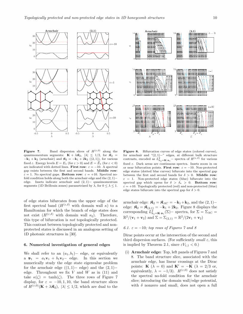
Figure 7. Band dispersion slices of H(ε,0) along thequasimomentum segments: K + λK2, |λ| ≤ 1/2, for K2 =−k1 + k2 (armchair) and K2 = −k1 + 2k2 ((2, 1)), for various

fixed ε. Energy levels E = E? (for ε > 0) and E = E? (for ε < 0)are indicated with dotted lines. First row: ε = −10. A spectralgap exists between the first and second bands. Middle row:ε = 1. No spectral gaps. Bottom row: ε = +10. Spectral no-fold condition holds along both the armchair edge and the (2, 1)−edge. Insets indicate armchair and (2, 1)− quasimomentumsegments (1D Brillouin zones) parametrized by λ, for 0 ≤ λ ≤ 1.

of edge states bifurcates from the upper edge of thefirst spectral band (H(ε,δ) with domain wall κ) to aHamiltonian for which the branch of edge states doesnot exist (H(ε,δ) with domain wall κ\). Therefore,this type of bifurcation is not topologically protected.This contrast between topologically protected and non-protected states is discussed in an analogous setting of1D photonic structures in [30].

6. Numerical investigation of general edges

We shall refer to an (a1, b1)− edge, or equivalentlya v1 = a1v1 + b1v2− edge. In this section wenumerically study the edge state eigenvalue problemfor the armchair edge ((1, 1)− edge) and the (2, 1)−edge. Throughout we fix V and W as in (11) andtake κ(ζ) = tanh(ζ). The three rows of Figure 7display, for ε = −10, 1, 10, the band structure slicesof H(ε,0)(K + λK2), |λ| ≤ 1/2, which are dual to the

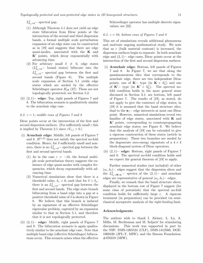
Figure 8. Bifurcation curves of edge states (colored curves),for armchair and “(2, 1)−” edges, at different bulk structurecontrasts, encoded as L2

k‖=K·v1− spectra of H(ε,δ) for various

fixed ε. Dark areas are continuous spectra. Insets zoom in onor near bifurcation points. First row: ε = −10. Non-protectededge states (dotted blue curves) bifurcate into the spectral gapbetween the first and second bands for δ > 0. Middle row:ε = 1. Non-protected edge states (blue) bifurcate into thespectral gap which opens for δ > δ? > 0. Bottom row:ε = +10. Topologically protected (red) and non-protected (blue)edge states bifurcate into the spectral gap for δ > 0.

armchair edge: K2 = KAC = −k1 +k2, and the (2, 1)−edge: K2 = K(2,1) = −k1 + 2k2. Figure 8 displays thecorresponding L2

k‖=K·v1(Σ)− spectra, for Σ = ΣAC =

R2/(v1 + v2) and Σ = Σ(2,1) = R2/(2v1 + v2)

6.1. ε = −10; top rows of Figures 7 and 8

Dirac points occur at the intersection of the second andthird dispersion surfaces. (For sufficiently small ε, thisis implied by Theorem 2.1, since εV1,1 < 0.)

(i) Armchair edge: Top, left panels of Figures 7 and8. The band structure slice, associated with thearmchair edge, has linear crossings at the Diracpoints: K (λ = 0) and K′ = −K (λ = 2/3 or,equivalently, λ = −1/3). H(ε,0) does not satisfythe spectral no-fold condition for the armchairslice; introducing the domain wall/edge potential,with δ nonzero and small, does not open a full

Topologically protected and non-protected edge states in 2D honeycomb structures 11

L2k‖=0− spectral gap.

(1) Although Theorem 4.1 does not yield an edgestate bifurcation from Dirac points at theintersection of the second and third dispersionbands, a formal multiple scale perturbationexpansion of an edge state can be constructedas in [19] and suggests that there are edgequasi-modes, associated with the K andK′ points, which decay exponentially withadvancing time.

(2) For arbitrary small δ 6= 0, edge states(L2

k‖=0− bound states) bifurcate into the

L2k‖=0− spectral gap between the first and

second bands (Figure 8). The multiplescale expansion of Section 5.1 yields edgestates which are seeded by the effectiveSchrodinger operator Heff (27). These are nottopologically protected; see Section 5.2.

(ii) (2, 1)− edge: Top, right panels of Figures 7 and8. The bifurcation scenario is qualitatively similarto the armchair edge case.

6.2. ε = 1; middle rows of Figures 7 and 8

Dirac points occur at the intersection of the first andsecond dispersion surfaces. (For sufficiently small ε thisis implied by Theorem 2.1 since εV1,1 > 0.)

(i) Armchair edge: Middle, left panels of Figures 7and 8. H(ε,0) does not satisfy the spectral no-foldcondition. Hence, for δ sufficiently small and non-zero, there is no L2

k‖=0− spectral gap between the

first and second spectral bands.

(1) As in the case ε = −10, the formal multi-ple scale perturbation theory suggests the ex-istence of edge quasi-modes with complex fre-quencies, which decay exponentially with ad-vancing time.

(2) Numerical simulations show that there is athreshold value, δ? > 0, such that for δ > δ?,there is an L2

k‖=0− spectral gap between the

first and second bands. The edge state branchbifurcating from a band edge into a gap at apositive threshold value of δ is shown in Figure8. We believe that this branch is inducedby an eigenstate of an effective Schrodingereigenvalue problem, captured by an expansionsimilar to that in Section 5.1, and thereforethat it is not topologically protected.

(ii) (2, 1)− edge: Middle, right panels of Figures 7and 8. The bifurcation scenario is again qualita-tively similar to the armchair edge case. Note thatmultiple band edge (effective Schrodinger) bifurca-tions occur. This scenario arises when the effective

Schroedinger operator has multiple discrete eigen-values; see [32].

6.3. ε = 10; bottom rows of Figures 7 and 8

This set of simulations reveals additional phenomenaand motivate ongoing mathematical study. We notethat as ε (bulk material contrast) is increased, thedispersion surfaces begin to separate. In both armchairedge and (2, 1)− edge cases, Dirac points occur at theintersection of the first and second dispersion surfaces.

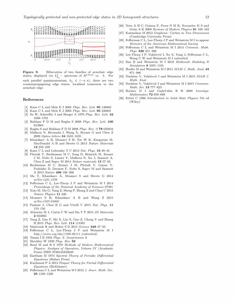
(i) Armchair edge: Bottom, left panels of Figures7 and 8. In Figure 7, we see that along thequasimomentum slice that corresponds to thearmchair edge, there are two independent Diracpoints, one of K− type (in K + Λ∗h) and oneof K′− type (in K′ + Λ∗h). The spectral no-fold condition holds in the more general sensediscussed in Section 3.1; see bottom, left panelof Figure 7. The results of [19], as stated, donot apply to give the existence of edge states; in[19] it is assumed that the band structure slice,dual to the v1− edge intersects at most one Diracpoint. However, numerical simulations reveal twofamilies of edge states, associated with K andK′ points, corresponding to counterpropagatingarmchair edge states; see Figure 9. We believethat the analysis of [19] can be extended to givea rigorous construction of these states (article inpreparation). These two branches are seeded bythe degenerate zero-energy eigenstate of a 4 × 4block-diagonal system of Dirac operators.

(ii) (2, 1)− edge: Bottom, right panels of Figures 7and 8. The spectral no-fold condition holds andwe expect the general theorem of [19] to apply.

Further numerical studies (not included) of other(a1, b1)− edges suggest that the dispersion slices andthe L2

k‖=K·v1− spectra of the (2, 1)− and armchair

edges are representative of general (a1, b1)− edges.Finally, we remark that the band structure slices,

displayed in the bottom row of Figure 7 suggest (forsome class of potentials) that the spectral no-foldcondition holds for sufficiently large ε. A rigoroustreatment (in preparation) can be provided via semi-classical asymptotic analysis of the tight-binding limit.

Acknowledgments

The authors wish to thank I. Aleiner, L. Lu, A.Millis, M. Rechtsman and M. Soljacic for stimulatingdiscussions. This work was supported in part bythe NSF: DMS-1265524 (CLF), DMS-1412560, DGE-1069420 (JPL-T, MIW); and the Simons Foundation:#376319 (MIW).

Topologically protected and non-protected edge states in 2D honeycomb structures 12

Figure 9. Bifurcation of two families of armchair edgestates, displayed via L2

k‖− spectrum of H(10,5) vs. δ. For

each parallel quasimomentum, k‖ ∈ (−π, π), there are twocounterpropagating edge states, localized transverse to thearmchair edge.

References

[1] Kane C L and Mele E J 2005 Phys. Rev. Lett. 95 146802[2] Kane C L and Mele E J 2005 Phys. Rev. Lett. 95 226801[3] Su W, Schrieffer J and Heeger A 1979 Phys. Rev. Lett. 42

1698–1701[4] Haldane F D M and Raghu S 2008 Phys. Rev. Lett. 100

013904[5] Raghu S and Haldane F D M 2008 Phys. Rev. A 78 033834[6] Malkova N, Hromada I, Wang X, Bryant G and Chen Z

2009 Optics letters 34 1633–1635[7] Khanikaev A B, Mousavi S H, Tse W K, Kargarian M,

MacDonald A H and Shvets G 2013 Nature Materials12 233–239

[8] Kane C L and Lubensky T C 2013 Nat. Phys. 10 39–45[9] Plotnik Y, Rechtsman M C, Song D, Heinrich M, Zeuner

J M, Nolte S, Lumer Y, Malkova N, Xu J, Szameit A,Chen Z and Segev M 2014 Nature materials 13 57–62

[10] Rechtsman M C, Zeuner J M, Plotnik Y, Lumer Y,Podolsky D, Dreisow F, Nolte S, Segev M and SzameitA 2013 Nature 496 196–200

[11] Ma T, Khanikaev A, Mousavi S and Shvets G 2014arXiv:1401.1276

[12] Fefferman C L, Lee-Thorp J P and Weinstein M I 2014Proceedings of the National Academy of Sciences 07391

[13] Xiao M, Ma G, Yang Z, Sheng P, Zhang Z and Chan C 2015Nature Physics 11 240

[14] Mousavi S H, Khanikaev A B and Wang Z 2015arXiv:1507.03002

[15] Paulose J, Chen B G and Vitelli V 2015 Nat. Phys. 11153–156

[16] Ablowitz M J, Curtis C W and Ma Y P 2015 2D Materials2 024003

[17] Yang Z, Gao F, Shi X, Lin X, Gao Z, Chong Y and ZhangB 2015 Phys. Rev. Lett. 114 114301

[18] Susstrunk R and Huber S D 2015 Science 349 47–50[19] Fefferman C L, Lee-Thorp J P and Weinstein M I

http://arxiv.org/abs/1506.06111 (submitted)[20] Tamm I E 1932 Phys. Z. Sowjetunion 1[21] Shockley W 1939 Phys. Rev. 56[22] Reed M and B S 1978 Methods of Modern Mathematical

Physics: Analysis of Operators, Volume IV (AcademicPress) ISBN 9780125850049

[23] Eastham M 1974 Spectral Theory of Periodic DifferentialEquations (Hafner Press)

[24] Kuchment P A 2012 Floquet Theory for Partial DifferentialEquations (Birkhauser)

[25] Fefferman C L and Weinstein M I 2012 J. Amer. Math. Soc.25 1169–1220

[26] Neto A H C, Guinea F, Peres N M R, Novoselov K S andGeim A K 2009 Reviews of Modern Physics 81 109–162

[27] Katsnelson M 2012 Graphene: Carbon in Two Dimensions(Cambridge University Press)

[28] Fefferman C L, Lee-Thorp J P and Weinstein M I to appearMemoirs of the American Mathematical Society

[29] Fefferman C L and Weinstein M I 2014 Commun. Math.Phys. 326 251–286

[30] Lee-Thorp J P, Vukicevic I, Xu X, Yang J, Fefferman C L,Wong C W and Weinstein M I submitted

[31] Ilan B and Weinstein M I 2010 Multiscale Modeling &Simulation 8 1055–1101

[32] Hoefer M and Weinstein M I 2011 SIAM J. Math. Anal. 43971–996

[33] Duchene V, Vukicevic I and Weinstein M I 2015 SIAM J.Math. Anal.

[34] Duchene V, Vukicevic I and Weinstein M I 2015 Commun.Math. Sci. 13 777–823

[35] Borisov D I and Gadyl’shin R R 2008 Izvestiya:Mathematics 72 659–688

[36] Kittel C 1996 Introduction to Solid State Physics 7th ed(Wiley)