Big Fish in a Small Market: The impact of Export Price on Ex-vessel Price of Tuna in the Maldives Daniel V. Gordon a* Sinan Hussain b a Department of Economics, University of Calgary, 2500 University Drive NW Calgary Alberta, T2N 1N4 Canada, [email protected]* Corresponding
Transcript
Big Fish in a Small Market:
The impact of Export Price on Ex-vessel Price of Tuna in the Maldives
Daniel V. Gordona* Sinan Hussainb
a Department of Economics, University of Calgary, 2500 University Drive NW Calgary Alberta, T2N 1N4 Canada, [email protected] * Corresponding author
b Senior Research Officer, Fisheries Management Agency, Ministry of Fisheries and Agriculture, Maldives, [email protected]
The paper assesses the relationship between export and ex-vessel prices for tuna fish in the Republic of Maldives. The economic welfare of fishermen depends to a great extent on the price received for fish. The price of fish is set by external factors exogenous to fishermen. It is important in understanding the welfare of fishermen to understand the price links in the fish supply chain and the factors that impact the ex-vessel price of fish. This paper uses three models to investigate price determination in the ex-vessel market; ARMAX, inverse demand and margin equation. The results provide statistically important price relationships and price flexibilities on asymmetric export price effects.
Short Title: Ex-vessel Price Determination in the MaldivesKeywords Tuna, Price Flexibilities, Asymmetric Export Price EffectsJEL Classification Q22 · Q28
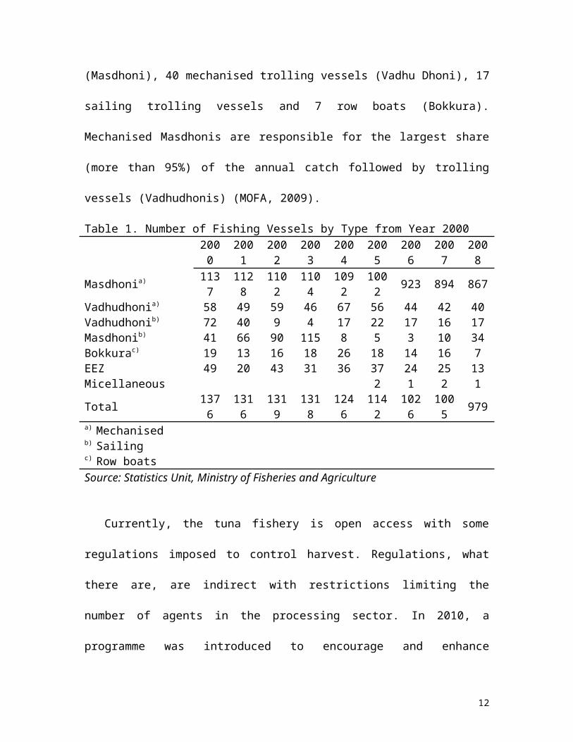
Currently, the tuna fishery is open access with some regulations imposed to control
harvest. Regulations, what there are, are indirect with restrictions limiting the number of
agents in the processing sector. In 2010, a programme was introduced to encourage and
enhance competition in the post-harvesting sector by allowing for Small and Medium
Enterprises (SME’s) to purchase skipjack tuna for processing. A total of 35 such
enterprises are now registered with the Ministry of Fisheries and Agriculture. Yellowfin
processors pay a royalty charge on harvest tonnage, which, of course, increases the cost
of processing.
A licensing scheme was introduced from November 2010 for vessels intending to
catch fish for the export market. This scheme could provide the basis for a future
management regime in the Maldives.
There are some concerns that the stocks of tuna may be declining with the
consequence of lower tuna harvest in the future. However, the Scientific Committee of
the Indian Ocean Tuna Commission suggests that stocks of skipjack do not appear
threatened, whereas stocks of yellowfin and bigeye are a concern.
3. Harvest and Process Data
9
The main data set represents the monthly value and quantity of tuna collected from
fishermen and the monthly value and quantity of exports of processed tuna for two
canneries over the period 2005 to 2010. As such the data will not only show historical
trends but also a comparative analysis across canneries. The data are used to calculate the
ex-vessel and export price by cannery and transformed to real values using the CPI.
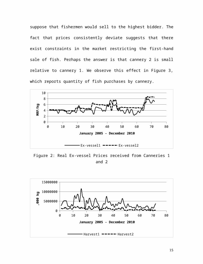
Figure 2 shows both historical trends and comparative effects for ex-vessel prices
received by fishermen for two canneries (1, 2) for the period January 2005 to December
2010. The graph shows that the trends in ex-vessel prices for each cannery are similar and
relatively flat over the period with some increase in real ex-vessel price near the end of
the series. Comparatively, ex-vessel prices received from cannery 2 appear generally
higher over the period and less variable.
It is surprising that we observe such sustained differences in ex-vessel prices across
canneries.6 One would suppose that fishermen would sell to the highest bidder. The fact
that prices consistently deviate suggests that there exist constraints in the market
restricting the first-hand sale of fish. Perhaps the answer is that cannery 2 is small relative
to cannery 1. We observe this effect in Figure 3, which reports quantity of fish purchases
by cannery.
6 We should keep in mind that the canneries do produce somewhat different products. They both produce frozen skipjack and yellowfin tuna and salted dried or canned skipjack, however, cannery 1 produces steamed skipjack loins.
10
0 10 20 30 40 50 60 70 800
2
4
6
8
10
Ex-vessel1 Ex-vessel2
January 2005 - December 2010
MR
F/k
g
Figure 2: Real Ex-vessel Prices received from Canneries 1 and 2
0 10 20 30 40 50 60 70 800
2000000
4000000
6000000
8000000
10000000
12000000
Harvest1 Harvest2
January 2005 - December 2010
,00
0 k
g
Figure 3: Harvest Collected by Processor 1 and 2
Figure 3 shows that cannery 1 is large relative to its rival. Cannery 2 seldom
purchases more than 2,000 tonnes of fish monthly compared to cannery 1 with purchases
as high as 12,000 tonnes of fish a month. What is interesting about the figure and speaks
directly to the income level of fishermen is that harvest has declined over the six-year
period. Real income to fishermen will decline unless the rise in the real price offsets the
fall in harvest.
11
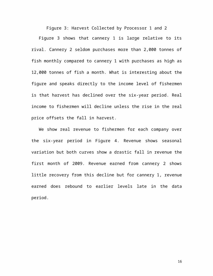
We show real revenue to fishermen for each company over the six-year period in
Figure 4. Revenue shows seasonal variation but both curves show a drastic fall in revenue
the first month of 2009. Revenue earned from cannery 2 shows little recovery from this
decline but for cannery 1, revenue earned does rebound to earlier levels late in the data
period.
0 10 20 30 40 50 60 70 800.00E+00
1.00E+07
2.00E+07
3.00E+07
4.00E+07
5.00E+07
Company1 Company2
January 2005 - December 2010
MR
F ,0
00
Figure 4: Real Revenue Fishermen from Cannery 1 and 2
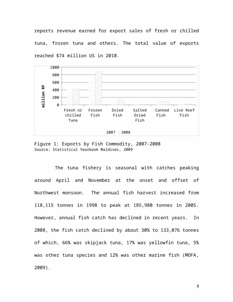
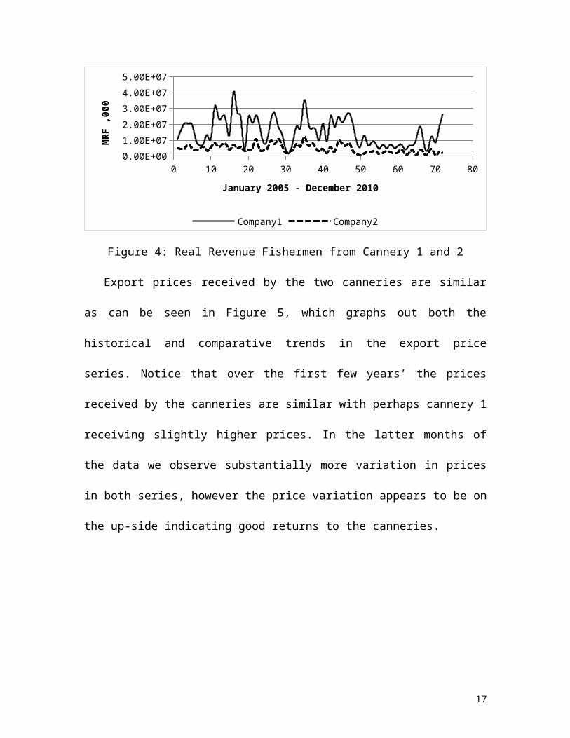
Export prices received by the two canneries are similar as can be seen in Figure 5,
which graphs out both the historical and comparative trends in the export price series.
Notice that over the first few years’ the prices received by the canneries are similar with
perhaps cannery 1 receiving slightly higher prices. In the latter months of the data we
observe substantially more variation in prices in both series, however the price variation
appears to be on the up-side indicating good returns to the canneries.
12
0 10 20 30 40 50 60 70 800
20406080
100
Export1 Export2
January 2005 - December 2010
MR
F/k
g
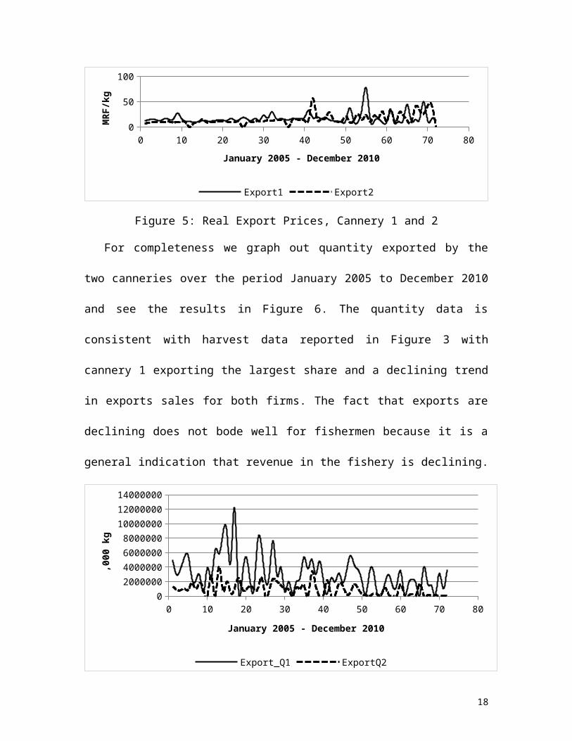
Figure 5: Real Export Prices, Cannery 1 and 2
For completeness we graph out quantity exported by the two canneries over the
period January 2005 to December 2010 and see the results in Figure 6. The quantity data
is consistent with harvest data reported in Figure 3 with cannery 1 exporting the largest
share and a declining trend in exports sales for both firms. The fact that exports are
declining does not bode well for fishermen because it is a general indication that revenue
in the fishery is declining.
0 10 20 30 40 50 60 70 800
2000000
4000000
6000000
8000000
10000000
12000000
14000000
Export_Q1 ExportQ2
January 2005 - December 2010
,00
0 k
g
Figure 6: Quantity Exported, Processor 1 and 2
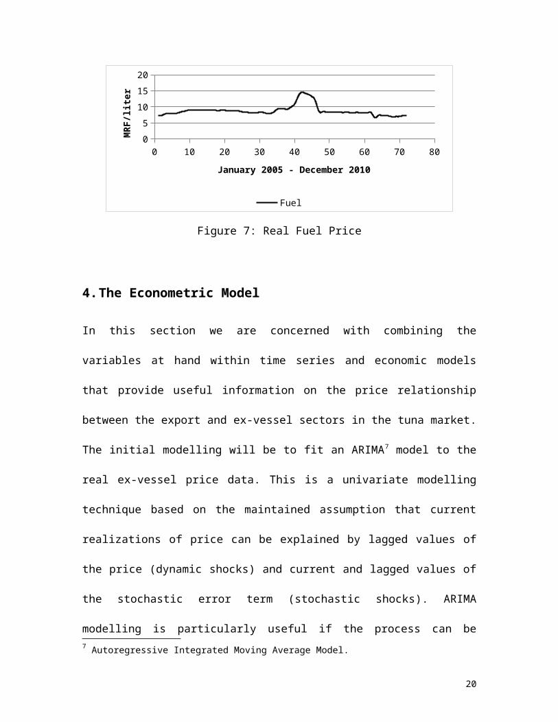
Figure 7 reports real fuel price over the six-year period of study. The trend in fuel
13
prices is surprisingly flat over much of the period with a large spike in prices during
2008. The Government controls most of the fuel supply in the Maldives through the State
Trading and Organization agency. The graph certainly represents a regulated policy on
fuel prices for the Maldives. It is worth noting that such a policy will distort incentives in
the market place. In this case, with fuel prices less than market value the subsidy will
encourage fishermen to exert more fishing effort than optimal. On efficiency grounds
lump sum income transfers are to be preferred to subsidies.
0 10 20 30 40 50 60 70 800
5
10
15
20
Fuel
January 2005 - December 2010
MR
F/li
ter
Figure 7: Real Fuel Price
4. The Econometric Model
In this section we are concerned with combining the variables at hand within time series
and economic models that provide useful information on the price relationship between
the export and ex-vessel sectors in the tuna market. The initial modelling will be to fit an
ARIMA7 model to the real ex-vessel price data. This is a univariate modelling technique
7 Autoregressive Integrated Moving Average Model.
14
based on the maintained assumption that current realizations of price can be explained by
lagged values of the price (dynamic shocks) and current and lagged values of the
stochastic error term (stochastic shocks). ARIMA modelling is particularly useful if the
process can be characterized as an autocorrelated series of unobserved shocks.8 The
ARIMA can be considered a reduced form price model for the purpose of short-run
forecasting and most importantly identification is maintained by only lagged dependent
and stochastic values appearing on the right-hand-side.9 Because the ARIMA model is
well identified a maximum likelihood estimator will generate consistent parameter
estimates. It is possible to augment the ARIMA price model by including exogenous
variables in specification for the purpose of improving forecasting possibilities and to
reduce forecast error.10 These extensions are defined as ARMAX or transfer function
models and for the case at hand we include the export price as a predetermined variable
that may impact the behaviour of ex-vessel price.11
The specification of the univariate price model is defined as:
Exvesse lt=αo+αex Exportt+∑i=1
p
γ i Exvessel t−i+∑j=1
q
θ j εt− j+εt (1)
where Exvesse lt is the ex-vessel price of fish in period t, Export t is export price in period
t,
p
iitVi Exvessel
1
represents the autoregressive (AR) component (dynamic shocks),
q
jjtj
1
represents the moving average (MA) component (stochastic shocks) and t is
8 For an excellent review of applied time series econometrics see, Enders (2004).9 For an interesting discussion of the first serious price forecasting model see, Gordon and Kerr (1997).10 The restriction on the exogenous variables requires that there be no feedback effect to the dependent variable (Enders, 2010)11 Seasonal and trend variables were also included in specification but did not statistically improve the forecast.
15
an iid random error term. Estimation of equation (1) is based on maximum likelihood
procedures.12
Selecting the correct lag specification for equation (1) is critical for generating an
estimated equation with good forecasting potential. Our research strategy is to evaluate
alternative AR and MA lag structures based on review of the autocorrelation and partial
autocorrelation functions with possible candidate specifications defined on testing iid
conditions in the stochastic error term using a Box-Lung Q-statistic. Among those
candidate specifications the preferred model is identified by measured BIC statistics.13
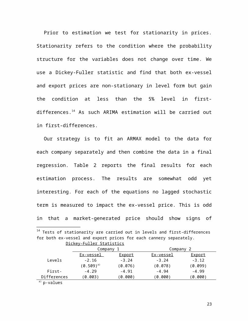
Prior to estimation we test for stationarity in prices. Stationarity refers to the
condition where the probability structure for the variables does not change over time. We
use a Dickey-Fuller statistic and find that both ex-vessel and export prices are non-
stationary in level form but gain the condition at less than the 5% level in first-
differences.14 As such ARIMA estimation will be carried out in first-differences.
Our strategy is to fit an ARMAX model to the data for each company separately and
then combine the data in a final regression. Table 2 reports the final results for each
estimation process. The results are somewhat odd yet interesting. For each of the
equations no lagged stochastic term is measured to impact the ex-vessel price. This is odd
in that a market-generated price should show signs of autocorrelated stochastic
behaviour. On the other hand, we do observe a statistically important one period
12 Estimation is carried out using STATA 11 software. 13 Bayesian Information Criteria.14 Tests of stationarity are carried out in levels and first-differences for both ex-vessel and export prices for each cannery separately. Dickey-Fuller Statistics
Company 1 Company 2Ex-vessel Export Ex-vessel Export
dynamic shock for each equation implying a one period lagged ex-vessel price is
important in setting current ex-vessel price. Finally, for company 1 and the combined
equation the current valued export price is an important determinant of the ex-vessel
price.
What do we make of such an equation? From our experience it is likely that the ex-
vessel price for tuna in the Maldives is a regulated price and not determined by purely
market forces. The ex-vessel price is set based on past behaviour implying that the
regulator is looking for stability in price trend but at the same time the price must respond
to real shocks in the export market. The problem is that because the ARMAX does not
capture the behaviour of the regulator, dynamic forecasts from such an equation are likely
to be biased.
Table 2: ARMAX of Ex-Vessel PriceCompany 1 Company 2 Total
Export Pricea) 0.1314(0.019)b)
0.0175(0.070)
0.0838(0.007)
AR−1 -0.2697(0.042)
-0.2529(0.036)
-0.2217(0.006)
Cons. 0.0137(0.530)
0.004(0.818)
0.007(0.560)
Obs. 59 66 125BICb) -9.839 -47.720 -63.153
a) First difference lagged twice export priceb) p-value in parentheses c) Bayesian Information Criteria
We carry out a dynamic forecast using the estimated combined ARMAX equation.
The dynamic forecast uses the actual values of the export price combined with the
predicted value of the AR component for forecasting. For purposes of presentation in-
sample forecasting (using only actual values of all variables) is carried out for the period
17
January 2005 to April 2010 with dynamic forecasts over the period May 2010 to the end
of the period. Figure 8 graphs out the forecast over the defined period. The graph shows
that the in-sample forecasts are very good but this is to be expected as we are merely
following the series. The important validation of the model is the dynamic forecast and
here we see that the model fails badly and is not able to follow the trend or pick up major
turning points in the series. Consequently, we must conclude that because the estimated
ARMAX does not model the behaviour of the regulator it fails as a useful short-run
forecast of ex-vessel price determination.
0 10 20 30 40 50 60 700
2
4
6
8
10
Exvesel Price Prediction
MR
F/k
g
Figure 8: Predicted Ex-vessel Price, dynamic after May 2010
We turn next to a structural approach to modelling ex-vessel price determination. We
follow Gordon (2011) in setting up the population regression model. Gordon argues that
econometric research should proceed by first setting out the full population regression
model. In this case, the full population regression model is the harvest-supply equation
and the demand equation for tuna. Then take this model to the data to write down the
final specification of the sample regression equation. Gordon argues that writing down
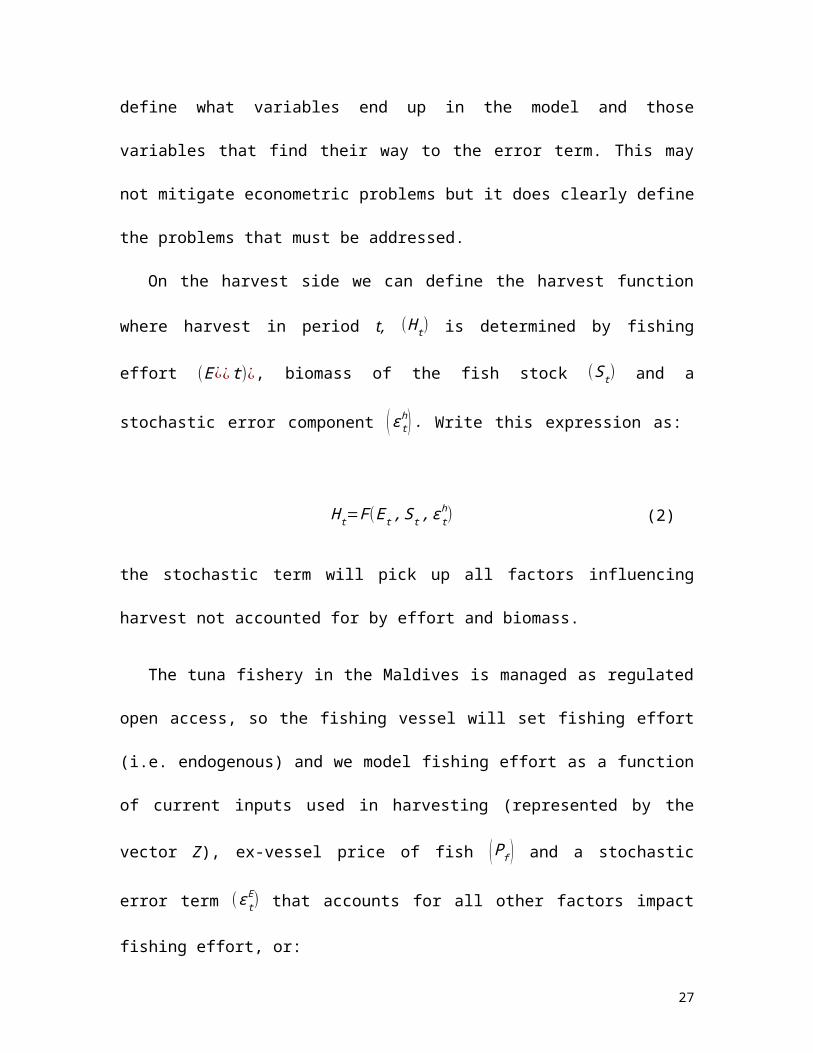
the population model allows the researcher to clearly define what variables end up in the
18
model and those variables that find their way to the error term. This may not mitigate
econometric problems but it does clearly define the problems that must be addressed.
On the harvest side we can define the harvest function where harvest in period t,
(H t) is determined by fishing effort (E¿¿ t )¿, biomass of the fish stock (St) and a
stochastic error component (εth ) . Write this expression as:
H t=F(Et , S t , εth) (2)
the stochastic term will pick up all factors influencing harvest not accounted for by effort
and biomass.
The tuna fishery in the Maldives is managed as regulated open access, so the fishing
vessel will set fishing effort (i.e. endogenous) and we model fishing effort as a function
of current inputs used in harvesting (represented by the vector Z), ex-vessel price of fish
( P f ) and a stochastic error term (εtE) that accounts for all other factors impact fishing
effort, or:
Et=I (Z t , Ptf , εt
E) (3)
Combining equations (2) and (3) we define the population harvest equation as:
H t=H (Ptf , Z t , S t , εt
h , εtE) (4)
Now we see that harvest is a function of the ex-vessel price of fish, a vector of harvest
input costs, the state of the biomass and stochastic error terms impacting harvest and
effort.
On the demand side the ex-vessel price of fish depends on harvest level, the export
price of fish (Pex), the cost of processing, transportation, etc. (represented by the vector
19
X) and other stochastic error factors impacting ex-vessel price (εf ). We write the
population ex-vessel price equation as:
Pf =g(H t , Ptex , X t , ε t
f ) (5)
Equations (4) and (5) represent the population structural model for the fishery. The
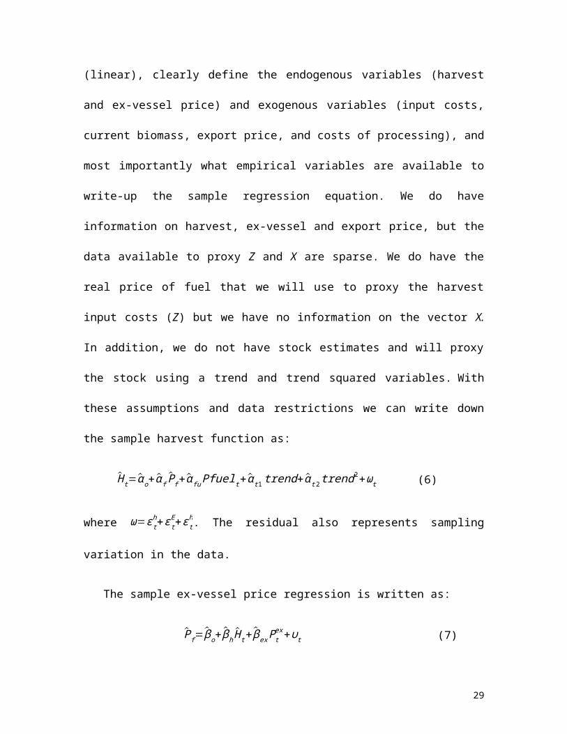
second stage is to make assumptions on the functional forms used in estimation (linear),
clearly define the endogenous variables (harvest and ex-vessel price) and exogenous
variables (input costs, current biomass, export price, and costs of processing), and most
importantly what empirical variables are available to write-up the sample regression
equation. We do have information on harvest, ex-vessel and export price, but the data
available to proxy Z and X are sparse. We do have the real price of fuel that we will use
to proxy the harvest input costs (Z) but we have no information on the vector X. In
addition, we do not have stock estimates and will proxy the stock using a trend and trend
squared variables. With these assumptions and data restrictions we can write down the
sample harvest function as:
H t=α o+α f Pf + α fu Pfuelt+ αt 1 trend+α t 2trend2+ωt (6)
where ω=εth+εt
E+ϵ th. The residual also represents sampling variation in the data.
The sample ex-vessel price regression is written as:
Pf = βo+ βh H t + βex Ptex+υ t (7)
where υt=εtf + X t βx+ϵ t
f . Again, the residual also represents sampling variation in the data.
20
Equations (6) and (7) represent the sample regression equation for the harvest and
price function, respectively. The price function is the equation of interest for this study
but because harvest is a right-hand-side endogenous variable a standard least squares
estimator will produce inconsistent estimates for all coefficients. We can address this
problem by using the exogenous variables in equation (5) to build an instrument to
replace harvest. The instrumental variables (IV) equation is written as:
H t=γ o+ γfu Pfuel t+γ t 1 trend+ γ t 2 trend2+ γex Ptex+ϵ t
iv (8)
Our estimation strategy is first to estimate equation (8) and predict harvest level
based on predetermined and exogenous variables. Predicted harvest satisfies the
conditions necessary for an IV variable i.e., correlated with actual harvest but not
correlated with the error term in equation (7). The IV is then used to replace actual
harvest in equation (7) prior to estimation.
Now it is important to state the conditions under which such a procedure will in fact
produce consistent estimates of the parameters in equation (7); for consistency what is
required is that the residual term ν t must not be correlated with any of the right-hand-side
variables in equation (7). So to be clear this says that processing costs must not be
correlated with harvest or export price, moreover the stochastic terms associated with
harvest and effort must also not be correlated with harvest or export price, and finally the
sample residual must also not be correlated with harvest or export price. In as much as
these conditions are satisfied our two-stage approach to estimation of equation (7) will
produce consistent estimates of the parameters of interest.15
15 In estimation we will include seasonal dummies in the harvest equation but not in the price equation. As seems reasonable, initial testing showed that the price relationship does not vary with the season.
21
The data available for analysis are panel series and we will use an instrumental
variable fixed effects estimator to recover the parameters of equation 7. The results of the
estimation are reported in Table 3.
Results reported in column 2 under heading (1) assume symmetry in ex-vessel price
response to increases and decreases in export price. The equation also includes the
instrumental variable for harvest and we control for seasonal effects. The data represent
log transforms and allows us to interpret the coefficients of interest as price flexibilities.
The price flexibility with respect to harvest is statistically important and valued at -0.19,
or in other words a 1% increase in harvest generates downward pressure on ex-vessel
price by 0.19%. The implication of this result is that the demand curve facing tuna
fishermen is downward sloping and indicates that increased fishing effort to harvest more
will be rewarded with lower ex-vessel prices, all else equal. This implies that the
Maldives’ tuna fishery is important in the world market for tuna and fishermen’s
behaviour impacts price. This is in contrast to a small fishing nation selling into a big
market and thus facing a horizontal demand curve for fish, or in this case fishermen’s
The export price flexibility assuming symmetry is small only 0.09% and statistically
valid at a 13% p-value. On the one hand this result is consistent with our earlier
comments on the ex-vessel price of fish being regulated and targeted with respect to the
export price. But the fact that the coefficient is not statistically important leads us to an
alternative strategy to categorized and separate export price shocks as either positive or
negative and asks the question is there asymmetric response in ex-vessel price to export
price shocks. The results for this extension are report in column three of Table 3 under
the heading (2). The results for the harvest coefficient are robust to the changes in
definition of export price but now we observe a substantial change in the impact of export
price on ex-vessel price. Either the positive and negative price shocks are strongly
statistically important but notice the positive shock is measured at 0.13% compared to the
negative shock at 0.15%, or in other words the ex-vessel price of fish is more responsive
to negative export price shocks than to positive export price shocks.
With only a very few downstream markets for tuna fish the firms are able to
manipulate the price and pass on negative price shocks compared to positive price
shocks. This does not seem all that surprising in a market where market power rests with
the canneries. Perhaps what is surprising is that the effect is less strong than expected and
in fact a simple test that the positive and negative coefficient are equal can only be
rejected at a 0.13 p-value. Consequently, there does appear to be serious market rigidity
23
in terms of export price shock pass through and the degree of monopsony pricing is
limited.
Finally we turn to a slightly different question and ask what is happening to the
margin overtime between export and ex-vessel price. The margin represents the
difference between the export price and ex-vessel price and we are interested in the trend
in the margin.16 If the margin is increasing over time this suggest that the players in the
export market are able to withhold a greater share of the final price with less recovered at
the vessel level. The margin model is a reduced form equation written as:
M t=α o+ βh H t+βex Ptex+βT Trend+βTT Tr end2+ε m (9)
Where M t is margin in period t, ε m is a stochastic error term picking up all other factors
not defined explicitly in the equation and all other variables are as previously defined.
The right hand side variables; harvest, export price and trend variables to proxy linear
and nonlinear trends in the margin, are predetermined in respect to the margin and a
fixed-effects panel data estimator will provide consistent estimates of the parameters. The
results of the estimation are reported in Table 4.
The main regression results are reported in the column headed (1) and show that
harvest has no important impact on the margin. The harvest variable is included in the
equation to proxy the supply side of the market and clearly the insignificant result tells us
that fishermen have little control over the margin. The export price variable assuming
symmetry in the margin response to a price change is strongly statistically significant
showing that size of the margin is positively related to export price. This suggests that the
market power to set the margin rests with the canneries. The trend and trend-squared
16 The margin could be defined with respect to ex-vessel prices lagged one or two periods but this makes little difference in the estimation. The correlation between the current margin and a one and two period lagged margin effect is 0.997 and 0.995, respectively
24
variables tell us that the margin has been falling over time but the rate of decline is
slowing down. The column headed (2) repeats the regression but allows for asymmetry in
export price shocks. This modification does not change the results for harvest or trend
variables but now we measure very similar coefficients on both the positive and negative
export price shocks. What this tells us is that the margin is maintained regardless of the
direction of change in export price.
25
Table 4: Margin Equation(1) (2)
Harvest 0.0873(0.151)
0.094(0.126)
Export Price 1.1369(0.00)
-
Export Price_pos - 1.343(0.00)
Export Price_neg. - 1.322(0.00)
Trend -0.0047(0.021)
-0.0048(0.018)
Trend2 0.00002(0.057)
0.00002(0.025)
Cons. -2.4634(0.012)
-2.474(0.011)
Obs. 128 128
The margin results are interesting in that as we would expect the many players on the
harvest supply side of the market have no impact on the margin. The market power to set
the margin is held by the few players in the export market i.e. canneries. Moreover the
canneries maintain the margin regardless of positive or negative price shocks at the
export level. Finally and a positive note for fishermen is that the margin has been
declining over time albeit the negative trend is decreasing.
26
5. Summary and Discussion
Purpose of research: The focus of this research is the derived demand for product from
export to first-hand market. This price approach is based on the theory of derived demand
where the export price of fish is exogenous in setting the ex-vessel price. The empirical
strategy was to first, build a univariate time series model (ARMAX) for the ex-vessel
price of fish for the purpose of dynamic forecasting. We include the export price of fish
as an exogenous variable in the model and control for seasonality and trend to improve
forecasting and to reduce forecast error. Second, recognizing the structural links between
the first-hand and export market we set up and specify a full demand and supply model
and then attempt to identify the inverse demand curve based on variables available for
empirical work. Finally, we ask the empirical question how has the margin between
export and ex-vessel prices varied over time.
Summary of results: Summary statistics show both declining harvest and exports
overtime. The consequence is that real income to fishermen will decline unless a rise in
the real ex-vessel price offsets the fall in harvest. In fact total real income to fishermen
has declined over the period of study except for the last few months of the period.
The ARMAX results show that no lagged stochastic term is measured to impact the ex-
vessel price. We do observe a statistically important one period dynamic shock for each
equation implying a one period lagged ex-vessel price is important in setting current ex-
vessel price. Also the current valued export price is an important determinant of the ex-
vessel price. These results indicate that the ex-vessel price for tuna in the Maldives is a
regulated price and not determined by purely market forces. The ex-vessel price is set
27
based on past behaviour implying that the regulator is looking for stability in price trend
but at the same time the price must respond to real shocks in the export market.
For the structural model and assuming symmetry in ex-vessel price response to
increases or decreases in export price we find negative price flexibility with respect to
harvest. This parameter is statistically important and valued at -0.19, or in other words a
1% increase in harvest generates downward pressure on ex-vessel price by 0.19%. The
implication of this result is that the demand curve facing tuna fishermen is downward
sloping and indicates that increased fishing effort to harvest more will be rewarded with
lower ex-vessel prices, all else equal. Cleary, the Maldives’ tuna fishery is important in
the world market for tuna and fishermen’s collective behaviour impacts ex-vessel price.
This is in contrast to a situation where a small fishing nation selling into a big market and
thus facing a horizontal demand curve for fish then the collective behaviour of fishermen
does not impact ex-vessel price.
We investigate asymmetry in the export price variable. We categorize and separate
export price shocks as either positive or negative and ask the question is there asymmetric
response in ex-vessel price to export price shocks. Both variables are important in ex-
vessel price setting. The positive shock has a measured flexibility of 0.13% compared to
the negative shock flexibility of 0.15%, or in other words the ex-vessel price of fish is
more responsive to negative export price shocks than to positive export price shocks.
With only a very few downstream markets for tuna fish, pass path through is stronger
for a negative price shock compared to a positive price shock. This does not seem all that
surprising in a market where market power rests with the canneries. Perhaps what is
surprising is that the effect is less strong than expected and in fact a simple test that the
28
positive and negative coefficient are equal can only be rejected at the 0.13 p-value.
Consequently, there does appear to be market rigidity in terms of export price shock pass
through but the degree of monopsony pricing seems limited.
The margin is an interesting variable and tells a story as to how much of the rent is
captured at the export level relative to the first-hand market. The margin results are what
we would expect in that the many players on the harvest-supply side of the market have
no impact on the margin. The market control to set the margin is held by the few players
in the export market i.e. canneries. Moreover the canneries maintain the margin
regardless of positive or negative price shocks at the export level. Finally, and a positive
note for fishermen, is that the margin has been declining over time albeit at a decreasing
rate.
Policy Discussion: On efficiency grounds policy regulators should avoid subsidies. In the
Maldives, fuel prices are regulated to try and stabilize an important input price to the
fishery. Regardless of the merits the consequence of subsidies is to distort the economic
incentives facing fishermen. For the case at hand, a subsidy that lowers the price of fuel
below market level results in increased fishing effort above the efficient level of
harvesting. If we define fishing effort by the number of fishermen then the consequence
of the subsidy is to encourage a greater number of fishermen than can be maintained
efficiently in the fishery. It may well be that fishermen in the Maldives are deserving of
increased income but on economic efficiency grounds this is best accomplished by direct
income transfers.
There is concern with overfishing of tuna stocks. Certainly, the results reported in
this study show a general decline in harvest levels and export quantities. Tuna are a
29
migratory fish stock and efforts to sustain the stock near optimal levels will require
international cooperation. Such cooperation will take time and success is uncertain. The
consequence is that the Maldives may face declining tuna stocks for some time. With a
measured price flexibility of -0.19% a fall in harvest will generate an ex-vessel price
increase but the increase will not be sufficient to offset the harvest decline and revenue to
fishermen will decline. This is a particularly serious problem for Maldives with a small
economy, alternative employment from the fishery is limited and likely outcome is that
existing fishermen will see their living standard decline.
The structure of the tuna market in Maldives is not unlike other small fishing nations
with many small first-hand suppliers of fish selling to only a few processors. Such a
structure sets the buying power to the processors and reduces the resource rent that could
go to the fishermen. There are two ways to counter this buyer market power; first, would
be to increase the number of processors, which will increase competition for raw fish and
push the ex-vessel price of fish upwards. On the other hand, a fishermen’s cooperative
could set up a single-desk seller operation where all fish harvested are marketed through
the single desk. Single desk selling could oppose the buying power of the canneries and
prices could be set in a cooperative manner to the benefit of both parties.
30
References
Asche, F., Menezes, R. And Dias, J.F. 2007 Price transmission in cross boundary supply chains Empirica 34:477-489.
Anderson, R. C. and Hafiz, A. (1991) How much bigeye in Maldivian yellowfin tuna catches? , IPTP.6
Azzam. A.M. 1999 Asymmetry and rigidity in farm-retail price transmission American Journal of Agricultural Economics 59:570-572.
Bjørndal, T. and D.V. Gordon, 2010, Cost and Earnings Study: Maldives. FAO Research Report, 33 pages.
Enders, W. 2010 Applied Econometric Time Series, 3rd Edition, Wiley.
Gordon, D.V. 1995 “Optimal Lag Length in Estimating Dickey-Fuller Statistics: An Empirical Note” Applied Economics Letters, 2:188-190.
Gordon, D.V. and W.A. Kerr. 1997 “Was the Babson Prize Deserved? An Enquiry into an Early Forecasting Model” Economic Modelling 14(3):417-433.
Gordon, D.V. ‘Price Modelling in the Canadian Fish Supply Chain with Forecasts and Simulations of the Ex-vessel Price of Fish’ Rome, FAO 2010a.
Gordon, D.V. 2011, Presentation to Warming Conference, Copenhagen: Denmark.
Gordon, D.V. ‘The Retail Demand Shift Variable and Marketing Cost Index: Fish Supply Chain in Canada: FAO Supply Chain Study’ Rome, FAO 2010b.
Hahn W.F. 1990 Price transmission asymmetry in pork and beef markets The Journal of Agricultural Economic Research 42:21-30.
DPND (2009) Maldives key Indicators - March 2009. Department of Planning and National Development, Republic of Maldives
MFAMR (2006a) Basic Fisheries Statistics - 2006. Ministry of Fisheries, Agriculture and Marine Resources, Republic of Maldives.
MOFA (2009) Basic Fisheries Statistics – 2009. Ministry of Fisheries and Agriculture, Republic of Maldives.
MPND (2004) 25 years of statistics of Maldives. Ministry of Planning and National Development
31
MPND (2004b) Vulnerability and Poverty Assessment 2, Ministry of Planning and National Development, Republic of Maldives.
Statistical yearbook Maldives 2009 Department of National Planning, Republic of Maldives,
Wohlgenant, M.K. 1985 competitive storage, rational expectations and short run food price determination American Journal of Agricultural Economics 67: 739-748.