BILINEAR ALGORITHMS AND ASIC ARCHITECTURES FOR FAST SIGNAL PROCESSING by Xingdong Dai Presented to the Graduate and Research Committee of Lehigh University in Candidacy for the Degree of Doctor of Philosophy in Computer Engineering Lehigh University 2008
Transcript
BILINEAR ALGORITHMS
AND
ASIC ARCHITECTURES
FOR
FAST SIGNAL PROCESSING
by
Xingdong Dai
Presented to the Graduate and Research Committee
of Lehigh University
in Candidacy for the Degree of
Doctor of Philosophy
in
Computer Engineering
Lehigh University
2008
UMI Number: 3314490
INFORMATION TO USERS
The quality of this reproduction is dependent upon the quality of the copy
submitted. Broken or indistinct print, colored or poor quality illustrations and
photographs, print bleed-through, substandard margins, and improper
alignment can adversely affect reproduction.
In the unlikely event that the author did not send a complete manuscript
and there are missing pages, these will be noted. Also, if unauthorized
copyright material had to be removed, a note will indicate the deletion.
®
UMI UMI Microform 3314490
Copyright 2008 by ProQuest LLC.
All rights reserved. This microform edition is protected against
unauthorized copying under Title 17, United States Code.
ProQuest LLC 789 E. Eisenhower Parkway
PO Box 1346 Ann Arbor, Ml 48106-1346
Approved and recommended for acceptance as a dissertation in partial fulfillment
of the requirements for the degree of Doctor of Philosophy.
AbAil £ 5 , 2.00$ Date
A/3A» 1 2Sj 2QO? Accepted Date
Dissertation Director Meghanad D. Wagh
Committee Members:
Meghanad D. Wagh
Bruce D. Fritchman
Zhiyuan Yan
\>A^>~ <-- Jf 0-3U&—
Bruce A. Dodson
QCu^-cte^J^ • "Sandeep Kumar
11
Acknowledgements
I wish to express appreciation for the members of my doctoral committee, the fac
ulty and staff at Lehigh University, friends and colleagues at LSI Corporation, and
family members here and abroad. This dissertation simply would not have been
possible, without your constant encouragement and unwavering support over many
years. Thank you very much for a wonderful experience. I will cherish it forever as
this research draws to a close.
I would like to thank my advisor, Dr. Meghanad D. Wagh, for his guidance during
my graduate study. Not only did he introduce me to the wonderful world of bilinear
algorithms on which this dissertation is focused, he has also shown me the virtue of
unselfishness. I remember many times how Dr. Wagh changed his busy schedule in
order to provide direction and support for this part-time student.
I would like to thank the members of my doctoral committee: Dr. Zhuyuan
Yan, Dr. Bruce D. Fritchman, Dr. Bruce A. Dodson and Dr. Sandeep Kumar. Each
contributed many stimulating ideas throughout this research. Their valuable feedback
greatly enhanced my dissertation.
During this work, friends and colleagues at LSI Corporation also generously lent
their support. From time to time, they substituted for me in conference calls or
meetings.
I want to thank my wife, Mingwei, for her cooperation and extreme patience during
long work days and late school nights. Last but not least, thanks to my parents for
their unconditional love and for providing me with a good education. You both were
my inspiration to accomplish this doctoral research work.
I am forever in your debt, xingdong.
in
iv
Contents
Acknowledgements iii
Abstract 1
1 Introduction 3
1.1 Motivation 3
1.2 Objective and contributions 7
1.3 Organization 11
2 ASIC methodology and mathematical background 15
2.1 Design methodology 16
2.1.1 General ASIC flow 16
2.1.2 ASIC for signal processing 18
2.2 Performance metric 20
2.3 Group theroy 25
2.3.1 Group definition 25
2.3.2 Cyclic and Hankel matrix products 26
2.4 Bilinear algorithm 28
2.4.1 Recursive decomposition 29
2.4.2 Order of computation 30
3 Discrete Hartley transform 35
3.1 Background and prior work 35
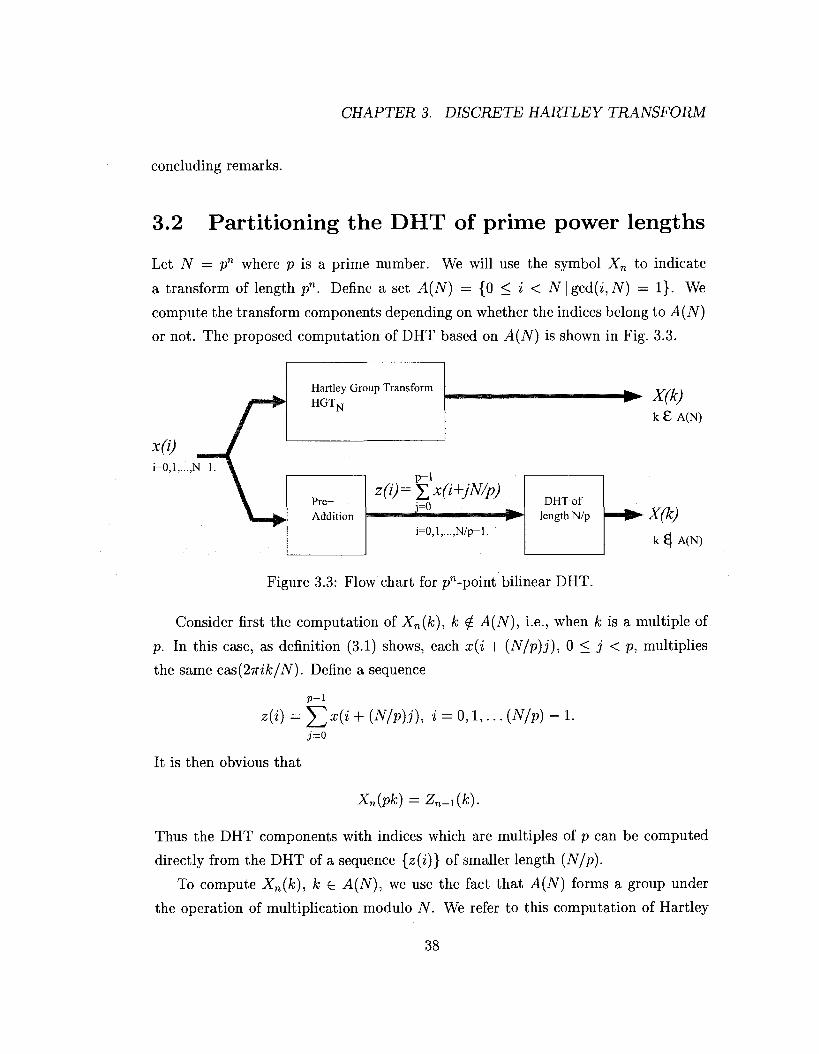
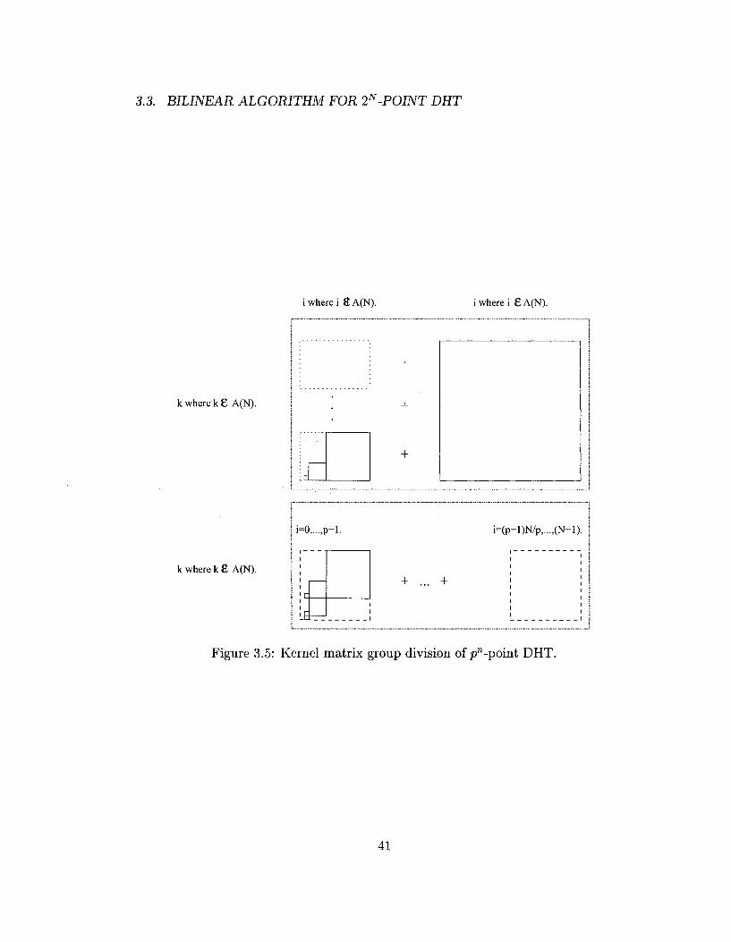
3.2 Partitioning the DHT of prime power lengths 38
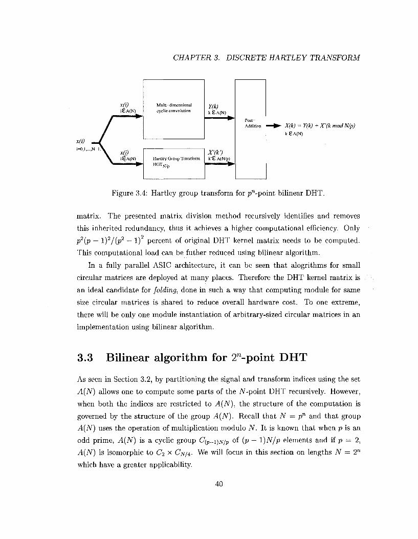
3.3 Bilinear algorithm for 2n-point DHT 40
v
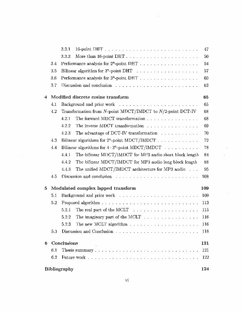
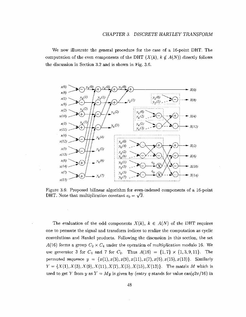
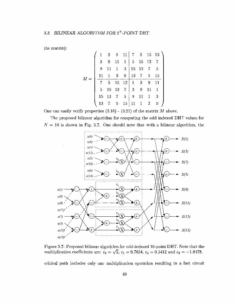
3.3.1 16-point DHT 47
3.3.2 More than 16-point DHT 50
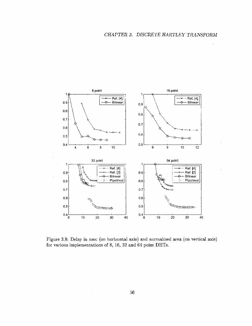
3.4 Performance analysis for 2n-point DHT 54
3.5 Bilinear algorithm for 3n-point DHT 57
3.6 Performance analysis for 3n-point DHT 60
3.7 Discussion and conclusion 63
4 Modified discrete cosine transform 65
4.1 Background and prior work 65
4.2 Transformation from iV-point MDCT/IMDCT to iV/2-point DCT-IV 68
4.2.1 The forward MDCT transformation 68
4.2.2 The inverse MDCT transformation 69
4.2.3 The advantage of DCT-IV transformation 70
4.3 Bilinear algorithms for 2"-point MDCT/IMDCT 72
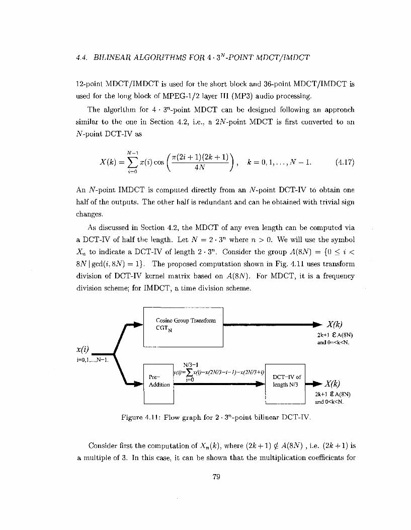
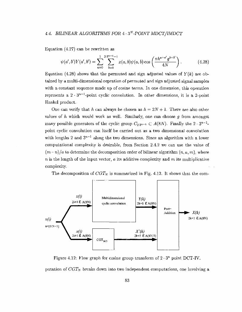
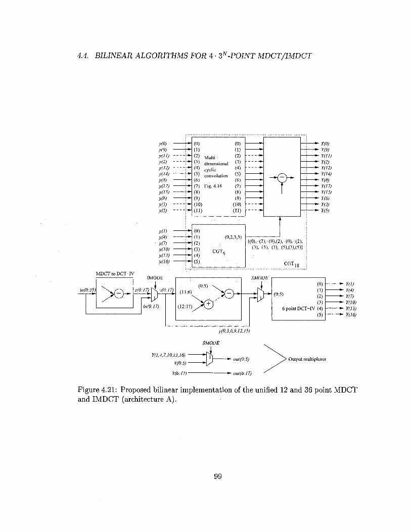
4.4 Bilinear algorithms for 4 • 3"-point MDCT/IMDCT 78
4.4.1 The bilinear MDCT/IMDCT for MP3 audio short block length 84
4.4.2 The bilinear MDCT/IMDCT for MP3 audio long block length 88
4.4.3 The unified MDCT/IMDCT architecture for MP3 audio . . . 95
4.5 Discussion and conclusion 108
5 Modulated complex lapped transform 109
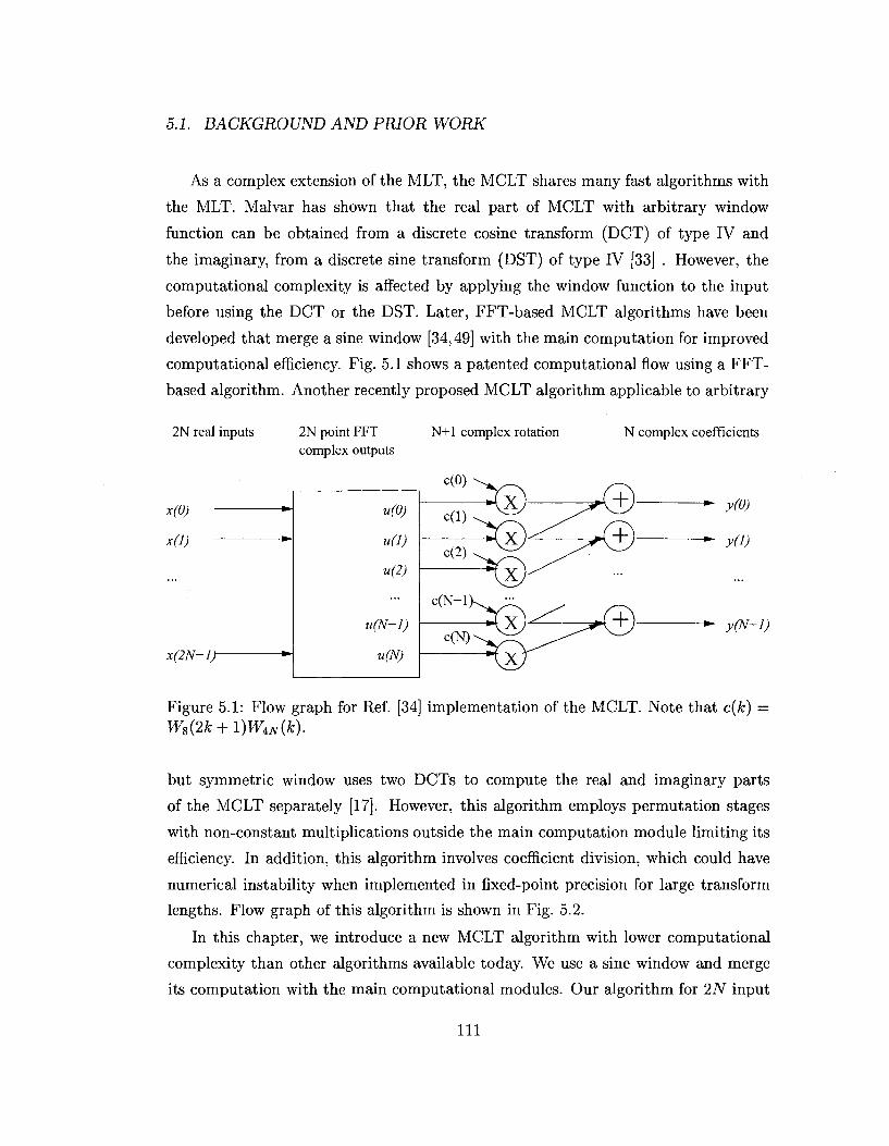
5.1 Background and prior work 109
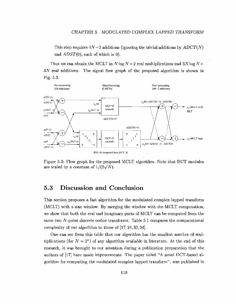
5.2 Proposed algorithm 113
5.2.1 The real part of the MCLT 115
5.2.2 The imaginary part of the MCLT 116
5.2.3 The new MCLT algorithm 116
5.3 Discussion and Conclusion 118
6 Conclusions 121 6.1 Thesis summary 121
6.2 Future work 122
Bibliography 124
VI
Vita 131
vn
viii
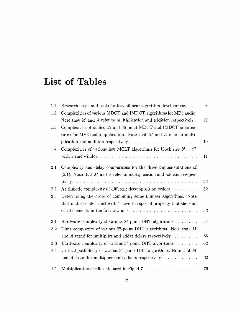
List of Tables
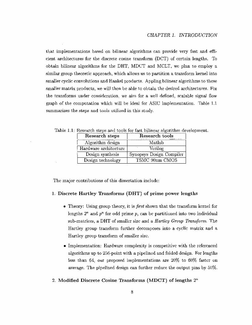
1.1 Research steps and tools for fast bilinear algorithm development. . . . 8
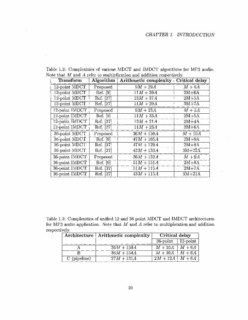
1.2 Complexities of various MDCT and IMDCT algorithms for MP3 audio.
Note that M and A refer to multiplication and addition respectively. 10
1.3 Complexities of unified 12 and 36 point MDCT and IMDCT architec
tures for MP3 audio application. Note that M and A refer to multi
plication and addition respectively. 10
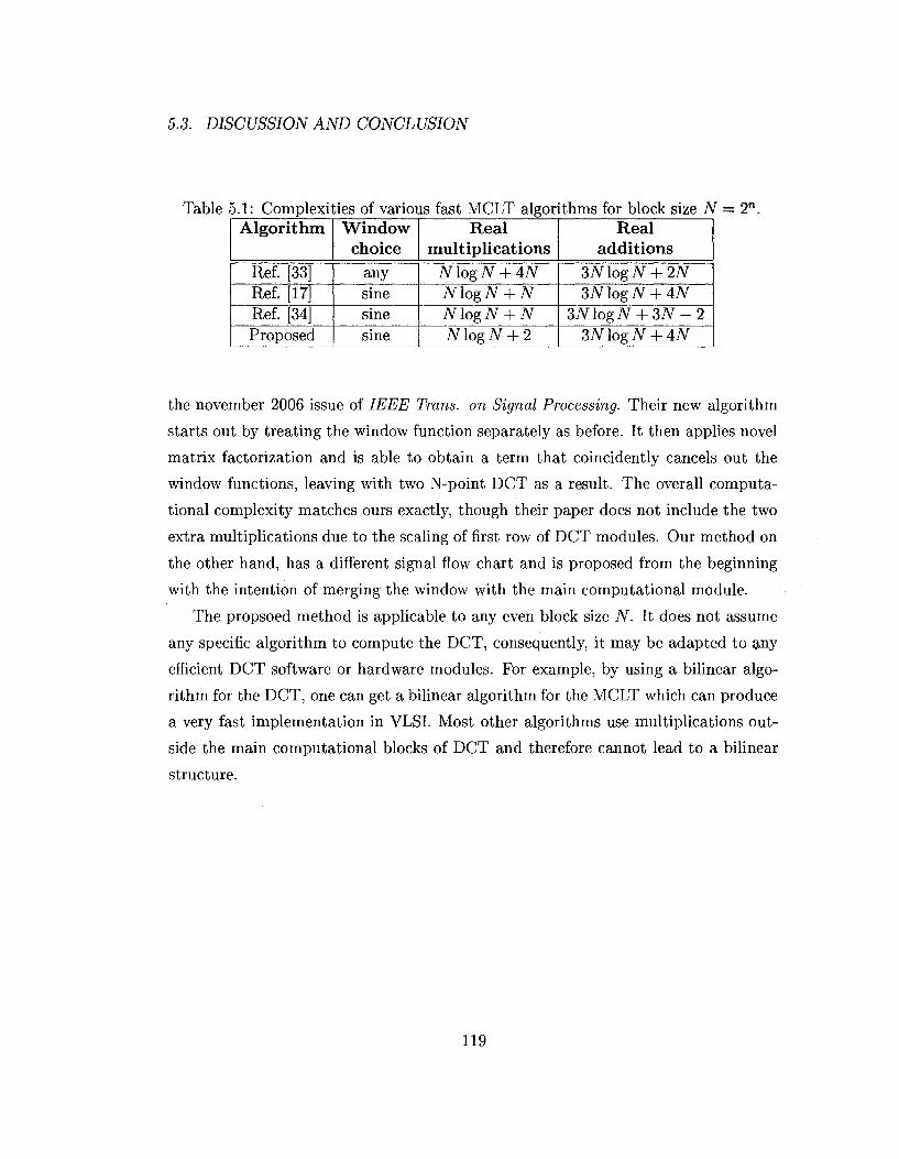
1.4 Complexities of various fast MCLT algorithms for block size N — 2n
with a sine window 11
2.1 Complexity and delay comparisons for the three implementations of
(2.1). Note that M and A refer to multiplication and addition respec
tively 23
2.2 Arithmetic complexity of different decomposition orders 32
2.3 Determining the order of combining some bilinear algorithms. Note
that matrices identified with * have the special property that the sum
of all elements in the first row is 0 33
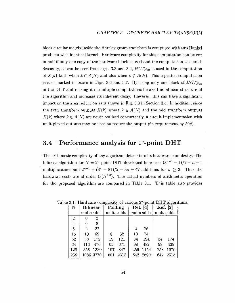
3.1 Hardware complexity of various 2"-point DHT algorithms 54
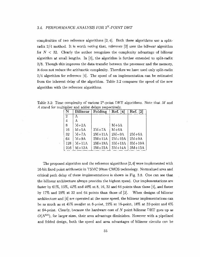
3.2 Time complexity of various 2ra-point DHT algorithms. Note that M
and A stand for multiplier and adder delays respectively. 55
3.3 Hardware complexity of various 3n-point DHT algorithms 62
3.4 Critical path delay of various 3n-point DHT algorithms. Note that M
and A stand for multipliers and adders respectively. 62
4.1 Multiplication coefficients used in Fig. 4.7 76
ix
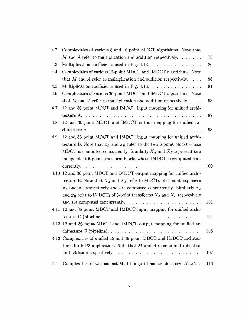
4.2 Complexities of various 8 and 16 point MDCT algorithms. Note that
M and A refer to multiplication and addition respectively 78
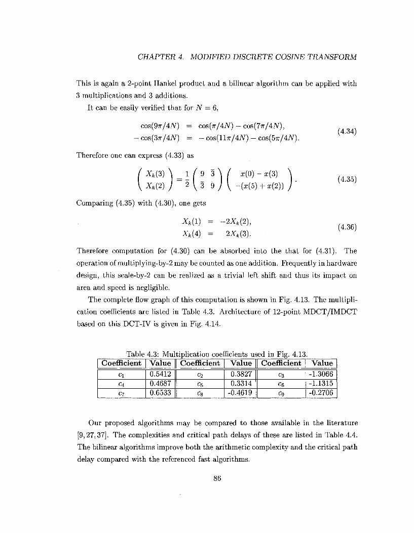
4.3 Multiplication coefficients used in Fig. 4.13 86
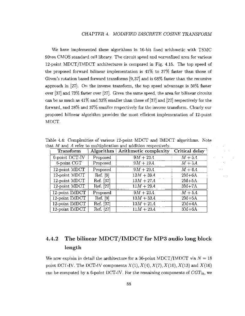
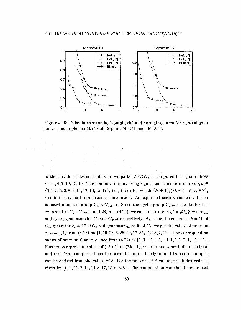
4.4 Complexities of various 12-point MDCT and IMDCT algorithms. Note
that M and A refer to multiplication and addition respectively. . . . 88
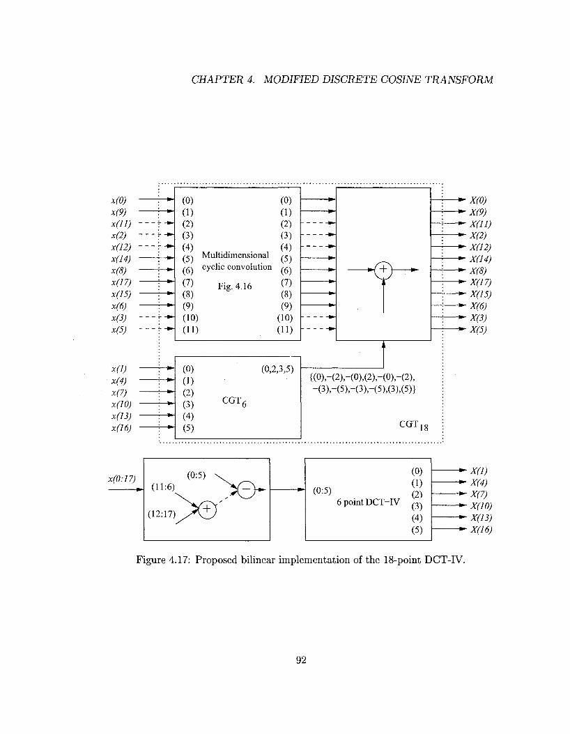
4.5 Multiplication coefficients used in Fig. 4.16 91
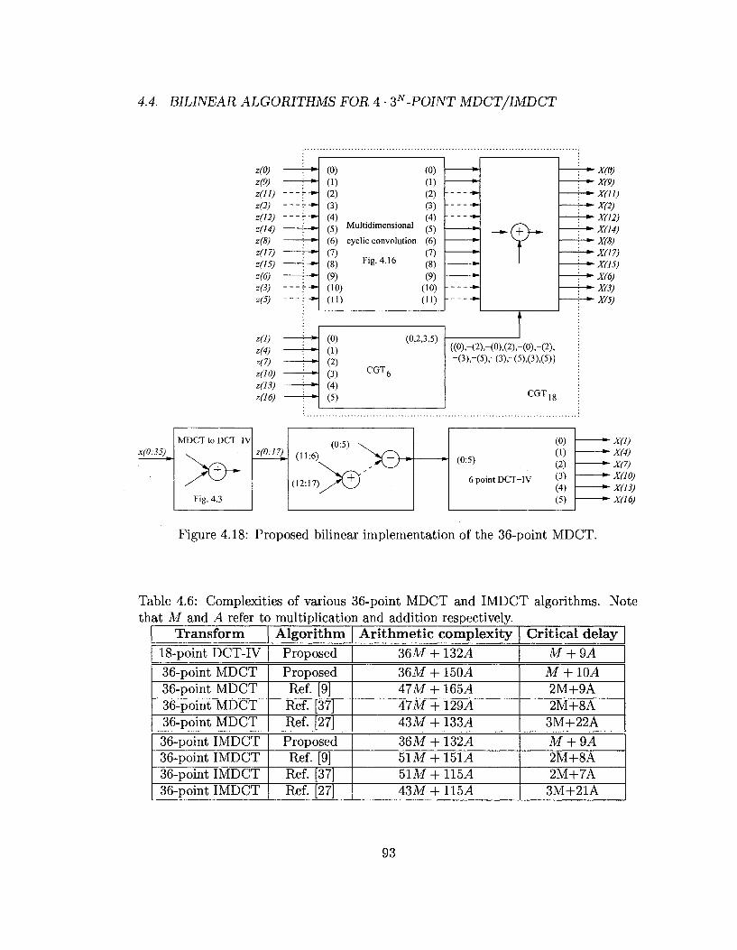
4.6 Complexities of various 36-point MDCT and IMDCT algorithms. Note
that M and A refer to multiplication and addition respectively. . . . 93
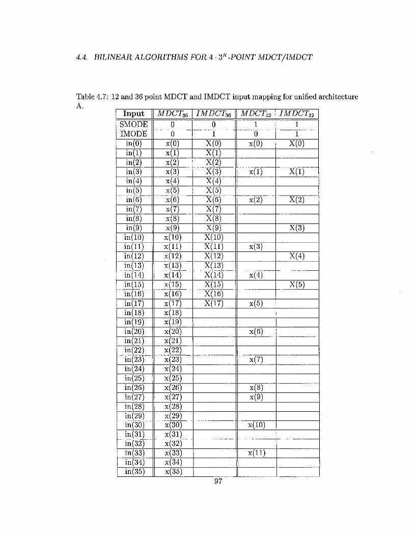
4.7 12 and 36 point MDCT and IMDCT input mapping for unified archi
tecture A 97
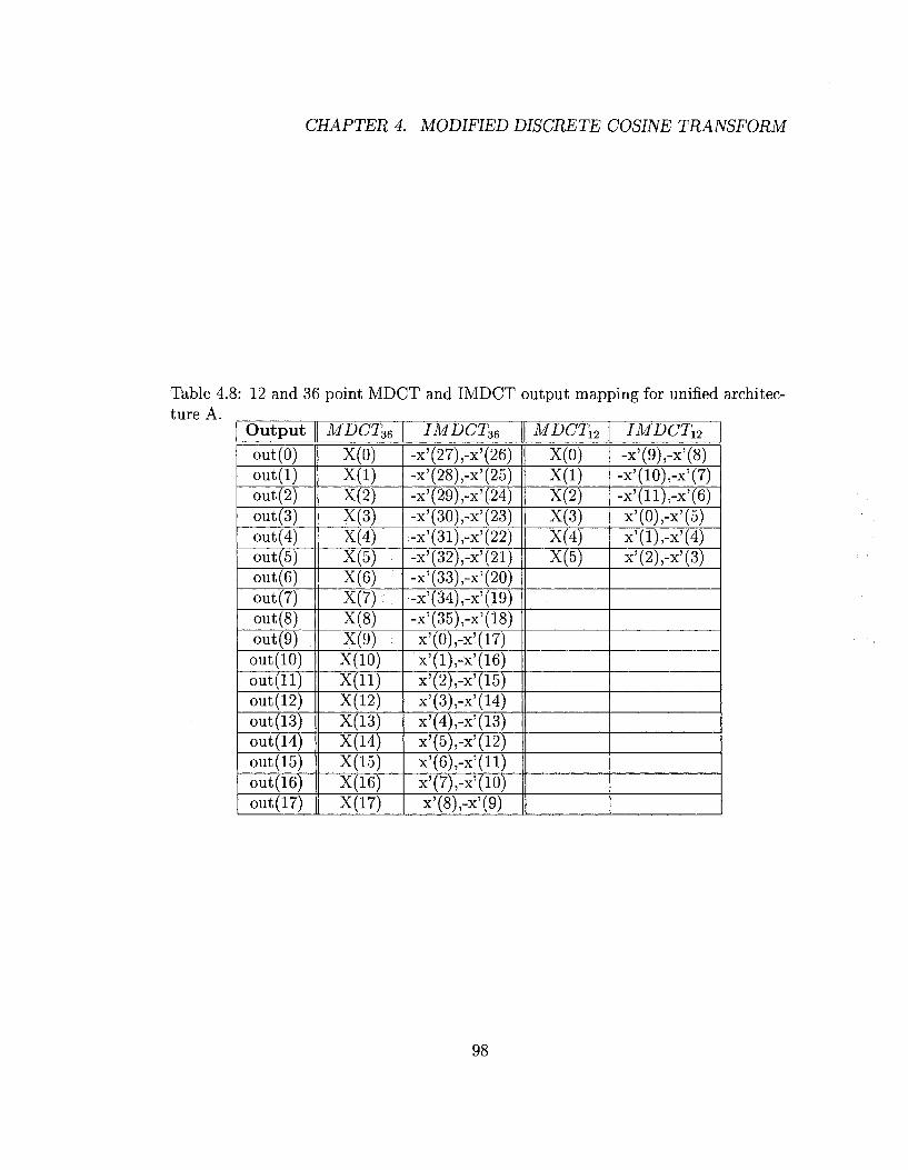
4.8 12 and 36 point MDCT and IMDCT output mapping for unified ar
chitecture A 98
4.9 12 and 36 point MDCT and IMDCT input mapping for unified archi
tecture B. Note that XA and XB refer to the two 6-point blocks whose
MDCT is computed concurrently. Similarly XA and XB represent two
independent 6-point transform blocks whose IMDCT is computed con
currently 100
4.10 12 and 36 point MDCT and IMDCT output mapping for unified archi
tecture B. Note that XA and XB refer to MDCTs of 6-point sequences
XA and xB respectively and are computed concurrently. Similarly x'A
and x'B refer to IMDCTs of 6-point transforms XA and XB respectively
and are computed concurrently 101
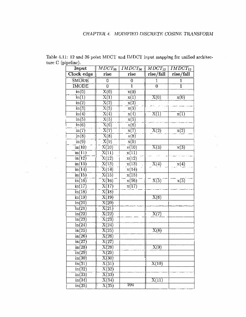
4.11 12 and 36 point MDCT and IMDCT input mapping for unified archi
tecture C (pipeline) 104
4.12 12 and 36 point MDCT and IMDCT output mapping for unified ar
chitecture C (pipeline) 106
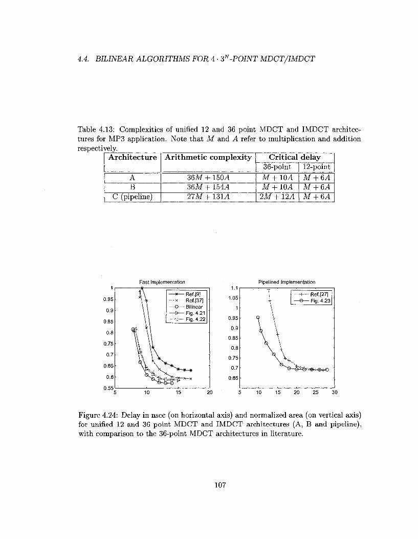
4.13 Complexities of unified 12 and 36 point MDCT and IMDCT architec
tures for MP3 application. Note that M and A refer to multiplication
and addition respectively. 107
5.1 Complexities of various fast MCLT algorithms for block size N — 2". 119
x
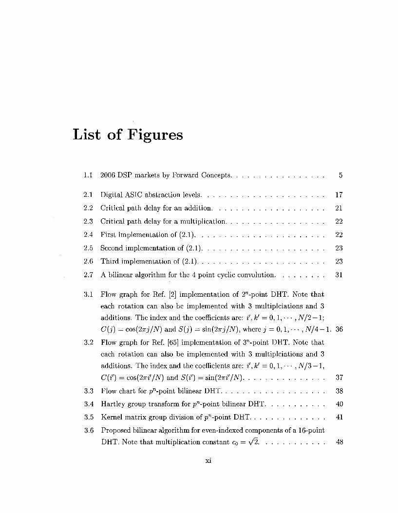
List of Figures
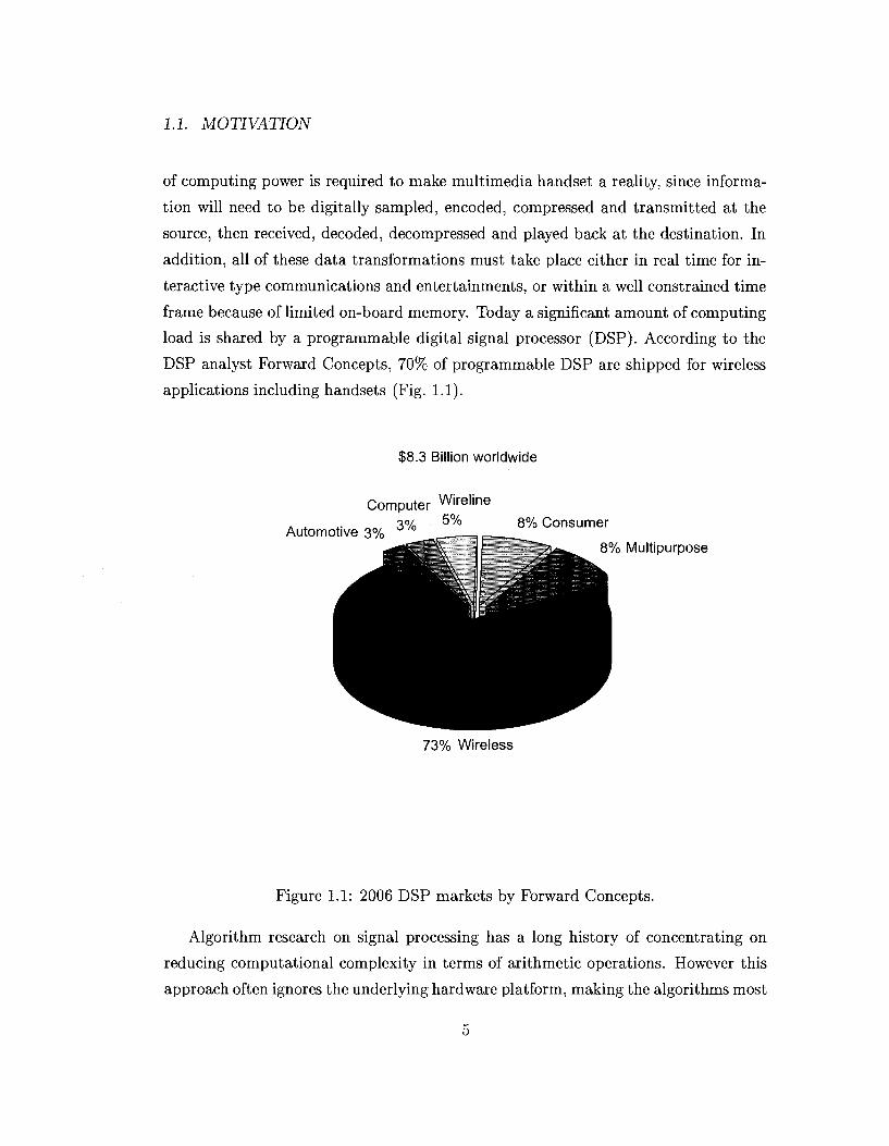
1.1 2006 DSP markets by Forward Concepts 5
2.1 Digital ASIC abstraction levels 17
2.2 Critical path delay for an addition 21
2.3 Critical path delay for a multiplication 22
2.4 First implementation of (2.1) 22
2.5 Second implementation of (2.1) 23
2.6 Third implementation of (2.1) 23
2.7 A bilinear algorithm for the 4 point cyclic convolution 31
3.1 Flow graph for Ref. [2] implementation of 2"-point DHT. Note that
each rotation can also be implemented with 3 multiplciations and 3
additions. The index and the coefficients are: i', k' — 0,1, • • • , N/2 — 1;
Critical delay M + 6A 2M+6A 2M+5A 3M+7A M + 5A 2M+5A 2M+4A 3M+6A
M + 10A 2M+9A 2M+8A
3M+22A M + 9A 2M+8A 2M+7A 3M+21A
Table 1.3: Complexities of unified 12 and 36 point MDCT and IMDCT architectures for MP3 audio application. Note that M and A refer to multiplication and addition respectively.
Architecture
A B
C (pipeline)
Arithmetic complexity
36M + 15CL4 36M + 154,4 27M + 1314
Critical delay 36-point M + 1CL4 M + 10A 2M + 12A
12-point M + 6A M + QA M + 6A
10
1.3. ORGANIZATION
Theory: Using trigonometric identities, it was shown that the window func
tion can be completely merged with the transform kernel so as to preserve
the bilinearity of the algorithm. The kernel can then be decomposed into a
discrete cosine transform and a discrete sine transform done concurrently.
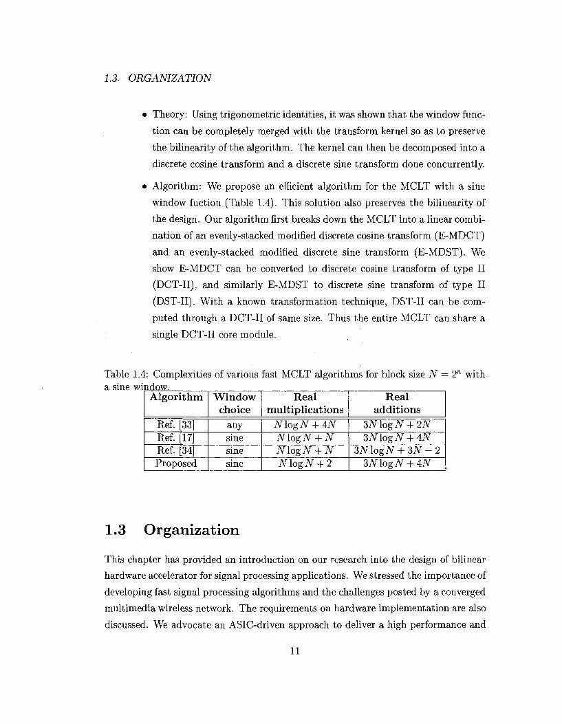
Algorithm: We propose an efficient algorithm for the MCLT with a sine
window fuction (Table 1.4). This solution also preserves the bilinearity of
the design. Our algorithm first breaks down the MCLT into a linear combi
nation of an evenly-stacked modified discrete cosine transform (E-MDCT)
and an evenly-stacked modified discrete sine transform (E-MDST). We
show E-MDCT can be converted to discrete cosine transform of type II
(DCT-II), and similarly E-MDST to discrete sine transform of type II
(DST-II). With a known transformation technique, DST-II can be com
puted through a DCT-II of same size. Thus the entire MCLT can share a
single DCT-II core module.
Table 1.4: Complexities of various fast MCLT algorithms for block size N = 2n with a sine window.
Algorithm
Ref. [33] Ref. [17] Ref. [34] Proposed
Window choice
any sine sine sine
Real multiplications
N\ogN + W iVlogJV + JV NlogN + N NlogN + 2
Real additions
3N\ogN + 2N 3JVlogJV + 4/V
3NlogN + 3N -2 3N\ogN + 4N
1.3 Organization
This chapter has provided an introduction on our research into the design of bilinear
hardware accelerator for signal processing applications. We stressed the importance of
developing fast signal processing algorithms and the challenges posted by a converged
multimedia wireless network. The requirements on hardware implementation are also
discussed. We advocate an ASIC-driven approach to deliver a high performance and
11
CHAPTER 1. INTRODUCTION
yet cost effective solution. Also presented in this chapter are our research objectives
and a summary of contributions.
In Chapter 2, we first discuss the ASIC design flow. Then concepts of group theory
and basic properties of the group are reviewed. This is followed by a detailed treat
ment of the bilinear algorithm. We show examples of bilinear algorithms for small
size cyclic convolutions and Hankel products. A bilinear algorithm for larger size
cyclic and Hankel matrix products can be derived by using small length algorithms
as building blocks. Since structured bilinear architecture has only one multiplication
on the critical path, the resulting ASIC circuit can be very fast in fixed point im
plementations. For a complex group structure, the order of computation can have
significant impact on the additive complexity. We discuss a procedure for determining
this computation order.
Bilinear algorithms for the DHT of prime power lengths are developed in Chapter
3. We investigate the structure of DHT kernel matrix using group A(pn) where p is
a prime number. This study leads to bilinear algorithms with a single multiplication
stage. Algorithm derivation and verification using MATLAB was carried out. The
new algorithms and two prior algorithms were implemented for a number of 2™ and
3" points and areas and critical path delays are compared.
In Chapter 4, we extend structured bilinear algorithms to 2n and 4 • 3" point
MDCT. Composite length MDCT algorithms of 4-3" points are the workhorse behind
the popularity of MPEG-1/2 layer III (MP3) audio format. The kernel matrix of
MDCT is rectangular (2" x 2"+1) and not square as in case of the DHT. With front-
end data massaging, we first transform the MDCT into a type-IV DCT. Both forward
and inverse transforms can be unified with a DCT-IV based algorithm. This has a
significant hardware implication since both encoder and decoder can now time-share
a single hardware. By taking advantages of the recursive structure inside a bilinear
algorithm, we propose three variations of unified hardware architecture for not only
the forward and inverse transforms, but also the short and long blocks. We show that
these proposed architectures offer superior performance over existing design solutions
and can be obtained with little area penalty.
Fast algorithm for Modulated complex lapped transform is developed in Chapter
12
1.3. ORGANIZATION
5. We obtain a bilinear algorithm for MCLT of lengths divisible-by-4 and with a sine
window. The real part of the MCLT is a modulated lapped transform (MLT). MLT
is related to the MDCT by first applying a window function to the input data. A
commonly used window is a sine window which preserves the perfect reconstruction.
The imaginary part of MCLT can be obtained by a modified discrete sine transform
(MDST) with windowed data. In most publications, this windowing function was
performed separately from the MDCT flow. A handful publications attempted to
merge the discrete computation steps. All met with limited success. Using trigono
metric identities, we show that the window function can be completely merged with
the transform kernel so as to preserve the bilinearity of the algorithm. The hardware
complexity of the new algorithm is computed and compared with four prior algo
rithms. It is shown that our proposed algorithm has the lowest overall complexity
and lowest multiplication requirements.
In the final chapter, the method and results of this research are summarized. To
obtain bilinear algorithms for the transforms under consideration, a group theoretic
approach can be proven successful in providing a fast VLSI architecture. The use of
group theory will allow us to partition a transform kernel of interest into smaller cyclic
and Hankel matrices. By applying bilinear algorithms on these matrix products, the
desired architectures can be obtained as a result. Future work is discussed on topics
of structured bilinear algorithm and algorithmic hardware acceleration.
13
CHAPTER 1. INTRODUCTION
14
Chapter 2
ASIC methodology and
mathematical background
This chapter provides the information about implementation techniques used as well
as the mathematical background required for this research. We start out with a re
view of ASIC design flow and metrics used to evaluate an implementation. Then the
concepts of group theory and basic properties of group used here are reviewed. This
is followed by a detailed treatment of the bilinear algorithm. We illustrate examples
of bilinear algorithms for small length cyclic convolutions and Hankel products. A
bilinear alogrithm for larger length cyclic and Hankel matrix products can be derived
using small length algorithms as building blocks. Since structured bilinear architec
ture has only one multiplication operation on the critical path, one can devise very
fast ASIC bilinear architectures in fixed-point implementations. For a complex group
structure, the ordering of computation can have a significant impact on the additive
complexity of the bilinear algorithm. We discuss a procedure for determining this
computation order.
15
CHAPTER 2. ASIC METHODOLOGY AND MATHEMATICAL BACKGROUND
2.1 Design methodology
2.1.1 General ASIC flow
Application specific integrated circuit (ASIC) has been the technology of choice for
many large volume applications. Many digital signal processing systems fit in this
category. For example, mobile phones are produced in very large numbers and re
quire high-performance circuits with respect to throughput and power consumption.
ASIC often has the performance advantages over digital signal processors (DSP) in
size, power and speed. These advantages are gained when area is optimized by elim
inating unnecessary and all unwanted functions that are part of a standard DSP. For
example, the instruction fetch-and-decode logic and interrupt handling circuits. As
such, ASIC circuits drive less capacitive load, resulting in less power dissipation and
better performance. In addition, the word precision and other design parameters can
be tailored to a specific application to provide optimum high-level performance.
ASIC however, is not without challenges. The most notables are the lack of the
programmability and ease of portability, and with that a longer design cycle. Since
ASIC implementations are literally set in stone, they can not be easily field-upgraded
and thus must be designed reliably on the first try. To achieve this objective, a
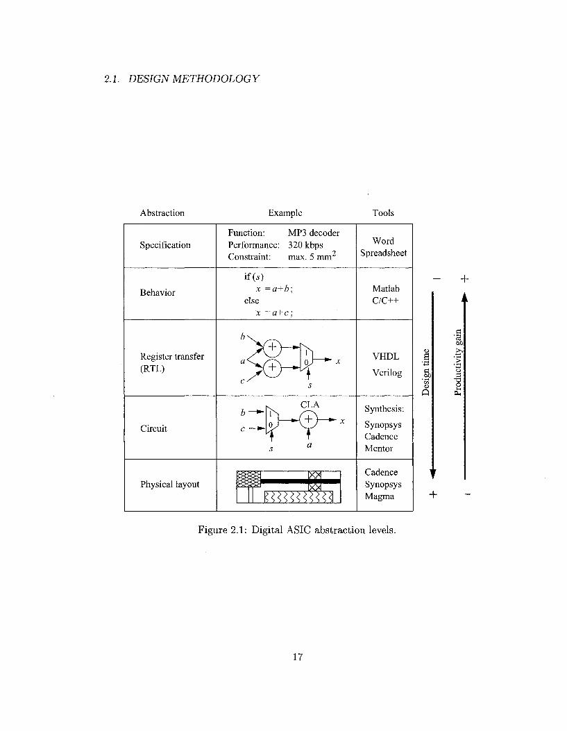
design ripples through a sequence of refinement stages called abstraction levels before
making its way into the silicon. The different design abstraction levels of a top-down
design methodology are illustrated in Fig. 2.1.
In a digital ASIC flow, the highest abstraction level is the specification level. It
defines the functionality, the performance and the constraints of target application.
Next is the behavioral level, where a design is often embodied by a system software
program that executes the function to be implemented in hardware. At the register
transfer level (RTL), the behavioral description is mapped to a well defined hardware
micro-architecture. The behavior and structure of a design is specified by describing
the operations that are performed on data as it flows between circuit inputs, outputs,
and clocked registers. At circuit level, different blocks of the hardware architecture
are committed to Boolean logic gates, latches, and flip-flops. For example, an adder
is committed to a specific implementation such as a carry propagation adder (CPA),
16
1. DESIGN METHODOLOGY
Abstraction Example Tools
Specification
Behavior
Register transfer (RTL)
Circuit
Physical layout
Function: MP3 decoder Performance: 320 kbps Constraint: max. 5 mm
if(s) x =a+b;
else x =a+c;
b—*~
c — * •
s
K. CLA
s a
if IX/1 m««««
Word Spreadsheet
Matlab C/C++
VHDL
Verilog
Synthesis:
Synopsys Cadence Mentor
Cadence Synopsys Magma
Figure 2.1: Digital ASIC abstraction levels.
17
CHAPTER 2. ASIC METHODOLOGY AND MATHEMATICAL BACKGROUND
a carry-lookahead adder (CLA), or a carry select adder (CSA) depending on the
availability of library cells. The circuit level is the stage where design synthesis is
performed to a specific technology node, such as TSMC 90nm CMOS process used in
this research. The final abstraction level before design sign-off is the physical layout
level. Here the design is linked to a specific technology and mask geometries are
derived. Simulation parameters such as wire resistance and parasitic capacitance are
extracted and fed back to a circuit simulator to ensure design can function at spec
ified performance level. Cross-talk analysis on electromigration is also performed to
determine if the device life time is sufficient for an application. Most often design will
iterate a few times between last two levels before a satisfactory solution is obtained.
We have seen that these abstraction levels offer opportunities to divide a compli
cated design process into smaller and more manageable tasks. A well-practiced ASIC
flow can significantly reduce the risk of introducing errors into the design. However it
is also this elaborated and fine-tuned procedure that demands significant effort and
time, which in turn often prolongs the design process. In order to shorten the schedule
without negatively impacting the quality of design, a frequently used improvement
technique is designing for reuse. This requires that during the design process, atten
tion must be paid to any iterative process within the scope. These iterative processes
can be extracted out as a macro or a core. They can be verified once and confi
dently applied many times. A systematic reuse of macros and cores provides the
quickest and most efficient approach to design ASIC [44]. In this dissertation, we will
show that our choice of design provides a natural way for design-for-reuse, As such,
a larger design can be quickly generated based on existing pre-verified blocks thereby
significantly shortening the design schedule.
2.1.2 ASIC for signal processing
Signal processing is fundamental to information processing. Generally the goal is
to reduce the information content in a signal to facilitate a decision about what
information the signal carries. In other instances, the aim is to retain the information
and to transform the signal into a form that is more suitable for transmission or
storage.
18
2.1. DESIGN METHODOLOGY
The major attributes of our ASIC design for signal processing are
• Standard cell based ASIC: Standard cell based ASIC, or cell-based IC (CBIC)
uses a collection of pre-designed logic cells to build a large complex circuit.
These logic cells are known as standard cells and include Boolean gates, flip-
flops and other complex modules such as multiplexers etc. The entire collection
is called a library. If building an ASIC is like building a house, the library is like
a Home Depot catalog, and the cells are equivalent to the lumber, bricks, nails
and tiles listed in the catalog. The advantage of this design approach is that
designers save time and reduce risk by using a pre-designed, pre-tested, and
pre-characterized standard cell library. ASIC designers can save their efforts to
focus on system functionality and high-level design tradeoffs.
• Fixed-point arithmetic: Early signal processors used fixed-point arithmetic and
often had far too short internal data length and far too small on-chip memory
to be efficient. Recent processors use floating-point arithmetic which is much
more expensive than fixed-point arithmetic in terms of power consumption,
execution time and chip area. In fact, these processors are not exclusively
aimed at DSP applications. Applications that typically require floating-point
arithmetic are three-dimension (3D) graphics and mechanical computer aided
design (CAD) applications. Fixed-point arithmetic is better suited for DSP
applications than floating-point arithmetic since good DSP algorithms require
high accuracy (long mantissa), but not the large dynamic signal range provided
by floating-point arithmetic. Further, the performance degradation due to non-
linearity (rounding of products) are less severe in fixed-point arithmetic.
• Direct mapping: DSP algothms rarely have many data dependent branching
operations. This makes them ideal candidates for the direct mapping technique
which involves creating a hardware structure that exactly matches with the sig
nal flow graph of the algorithm. This implementation technique is particularly
suitable for system with a fixed function, for example, digital filters and signal
transforms. Since direct mapping approach provides perfect match between the
19
CHAPTER 2. ASIC METHODOLOGY AND MATHEMATICAL BACKGROUND
DSP algorithm and the circuit architecture, it allows algorithm level design pa
rameter tradeoffs and tuning. It thus reduces the overall design time and leads
to a more reliable design.
2.2 Performance metric
The design space can be represented as a triplet:
(Function, Performance, Constraints).
That is to say a design has to deliver a function at a performance level under certain
constraints. For example, in signal processing, the function can be a digital filter
or a signal transform. The performance objectives are often time related, such as
signal sampling rate, or processor requirements such as clock frequency or MIPS.
The constraint targets, on the other hand, are frequently associated with cost, such
as chip area, power consumption, design schedule, or a combination. In general, a
successful design is about the trade off between the performance and the constraints
in order to realize some particular functions. In this dissertation, we are interested in
developing architectures for real-time DSP applications, where computations must be
completed within a given time frame (for example, the signal sample period). In such
applications, unacceptable errors occur if the time limit is exceeded. Consequently,
general purpose or DSP processors that rely on concepts such as memory management
units, cache etc., which may have a high throughput but not necessarily a guaranteed
time for each computation, are unacceptable. On the other hand, without these
features, general purpose and DSP processors cannot provide the necessary speed.
We therefore focus on ASIC solutions in this work.
Architecture speed is intrinsically tied to its critical path delay. Reducing overall
arithmetic complexity helps on the circuit area. However it does not address the
critical path delay directly. For algorithmic circuit, the critical path delay is attributed
to arithmetic operation speed and the number of operations on the signal path. This
implies that on the critical path, one needs to favor simple and fast operations such as
additions rather than more complex and slow operations such as multiplications. This
is especially important for fixed-point arithmetic, since intrinsic delay of a multiplier
20
2.2. PERFORMANCE METRIC
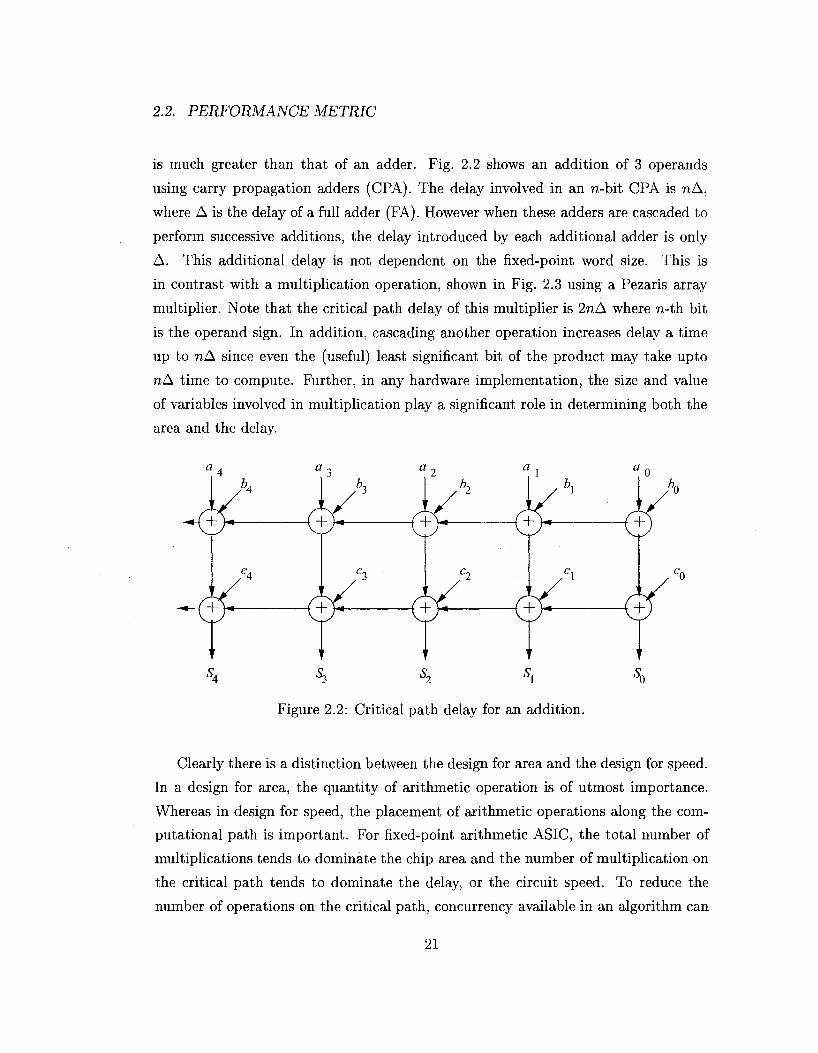
is much greater than that of an adder. Fig. 2.2 shows an addition of 3 operands
using carry propagation adders (CPA). The delay involved in an n-bit CPA is nA,
where A is the delay of a full adder (FA). However when these adders are cascaded to
perform successive additions, the delay introduced by each additional adder is only
A. This additional delay is not dependent on the fixed-point word size. This is
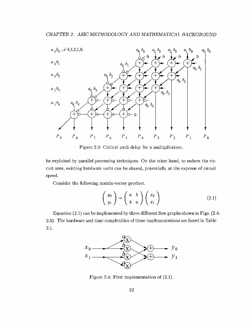
in contrast with a multiplication operation, shown in Fig. 2.3 using a Pezaris array
multiplier. Note that the critical path delay of this multiplier is 2nA where n-th bit
is the operand sign. In addition, cascading another operation increases delay a time
up to nA since even the (useful) least significant bit of the product may take upto
nA time to compute. Further, in any hardware implementation, the size and value
of variables involved in multiplication play a significant role in determining both the
area and the delay.
03 Oj Oj
Figure 2.2: Critical path delay for an addition.
Clearly there is a distinction between the design for area and the design for speed.
In a design for area, the quantity of arithmetic operation is of utmost importance.
Whereas in design for speed, the placement of arithmetic operations along the com
putational path is important. For fixed-point arithmetic ASIC, the total number of
multiplications tends to dominate the chip area and the number of multiplication on
the critical path tends to dominate the delay, or the circuit speed. To reduce the
number of operations on the critical path, concurrency available in an algorithm can
21
CHAPTER 2. ASIC METHODOLOGY AND MATHEMATICAL BACKGROUND
a {b0 ,i=4,3,2,l,0. a4 bQ a^bQ ^ bQ a, b Q aQ
0 1 .0 1.0 j ^ O
a4 bi (+>*- r+n- (+
7 J 6 J 5 " 4 J 3 J 2 " 1
Figure 2.3: Critical path delay for a multiplication.
t P.
be exploited by parallel processing techniques. On the other hand, to reduce the cir
cuit area, existing hardware units can be shared, potentially at the expense of circuit
speed.
Consider the following matrix-vector product.
a b
b a x0
Xl
(2.1)
Equation (2.1) can be implemented by three different flow graphs shown in Figs. (2.4-
2.6). The hardware and time complexities of these implementations are listed in Table
2.1.
Figure 2.4: First implementation of (2.1).
22
2.2. PERFORMANCE METRIC
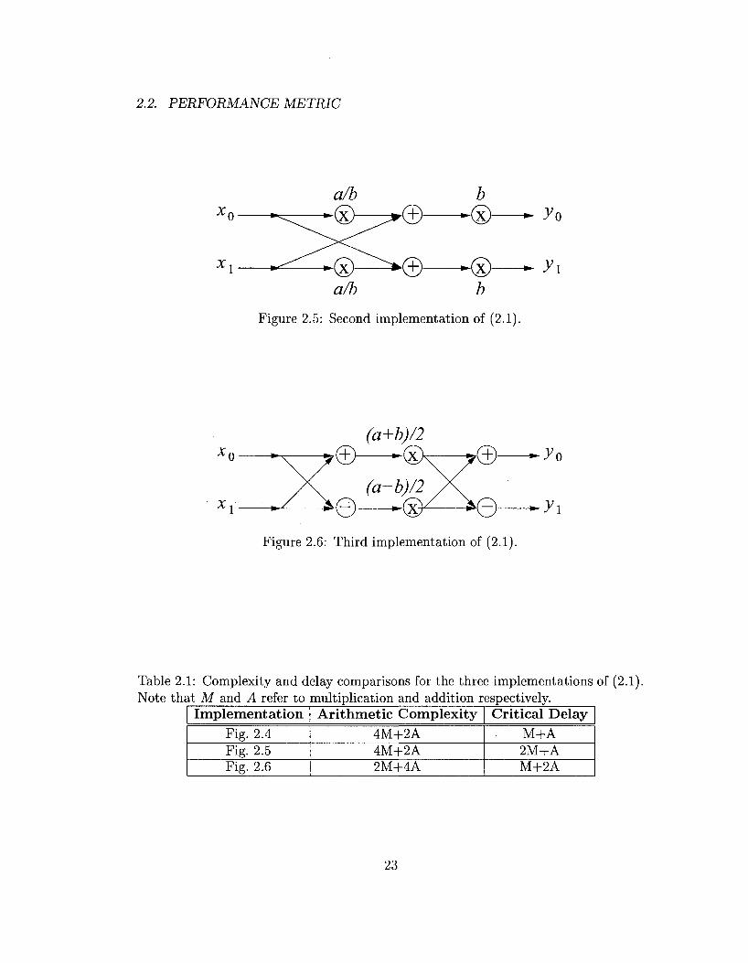
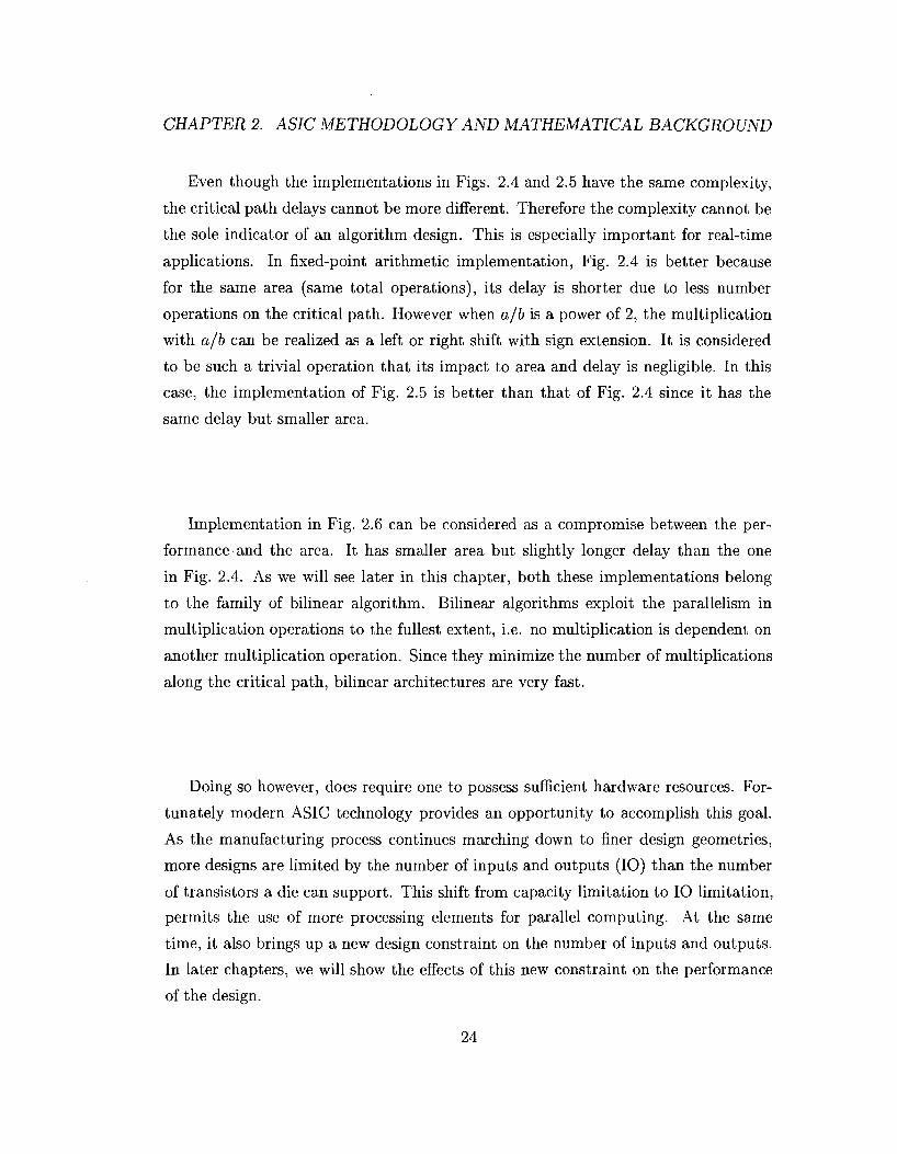
Figure 2.5: Second implementation of (2.1).
(a+b)/2
(a-b)/2 e—-s
Figure 2.6: Third implementation of (2.1).
Table 2.1: Complexity and delay comparisons for the three implementations of (2.1). Note that M and A refer to multiplication and addition respectively.
Implementation Fig. 2.4 Fig. 2.5 Fig. 2.6
Arithmetic Complexity 4M+2A 4M+2A 2M+4A
Critical Delay M+A 2M+A M+2A
23
CHAPTER 2. ASIC METHODOLOGY AND MATHEMATICAL BACKGROUND
Even though the implementations in Figs. 2.4 and 2.5 have the same complexity,
the critical path delays cannot be more different. Therefore the complexity cannot be
the sole indicator of an algorithm design. This is especially important for real-time
applications. In fixed-point arithmetic implementation, Fig. 2.4 is better because
for the same area (same total operations), its delay is shorter due to less number
operations on the critical path. However when a/b is a power of 2, the multiplication
with a/b can be realized as a left or right shift with sign extension. It is considered
to be such a trivial operation that its impact to area and delay is negligible. In this
case, the implementation of Fig. 2.5 is better than that of Fig. 2.4 since it has the
same delay but smaller area.
Implementation in Fig. 2.6 can be considered as a compromise between the per
formance and the area. It has smaller area but slightly longer delay than the one
in Fig. 2.4. As we will see later in this chapter, both these implementations belong
to the family of bilinear algorithm. Bilinear algorithms exploit the parallelism in
multiplication operations to the fullest extent, i.e. no multiplication is dependent on
another multiplication operation. Since they minimize the number of multiplications
along the critical path, bilinear architectures are very fast.
Doing so however, does require one to possess sufficient hardware resources. For
tunately modern ASIC technology provides an opportunity to accomplish this goal.
As the manufacturing process continues marching down to finer design geometries,
more designs are limited by the number of inputs and outputs (10) than the number
of transistors a die can support. This shift from capacity limitation to 10 limitation,
permits the use of more processing elements for parallel computing. At the same
time, it also brings up a new design constraint on the number of inputs and outputs.
In later chapters, we will show the effects of this new constraint on the performance
of the design.
24
2.3. GROUP THEROY
2.3 Group theroy
2.3.1 Group definition
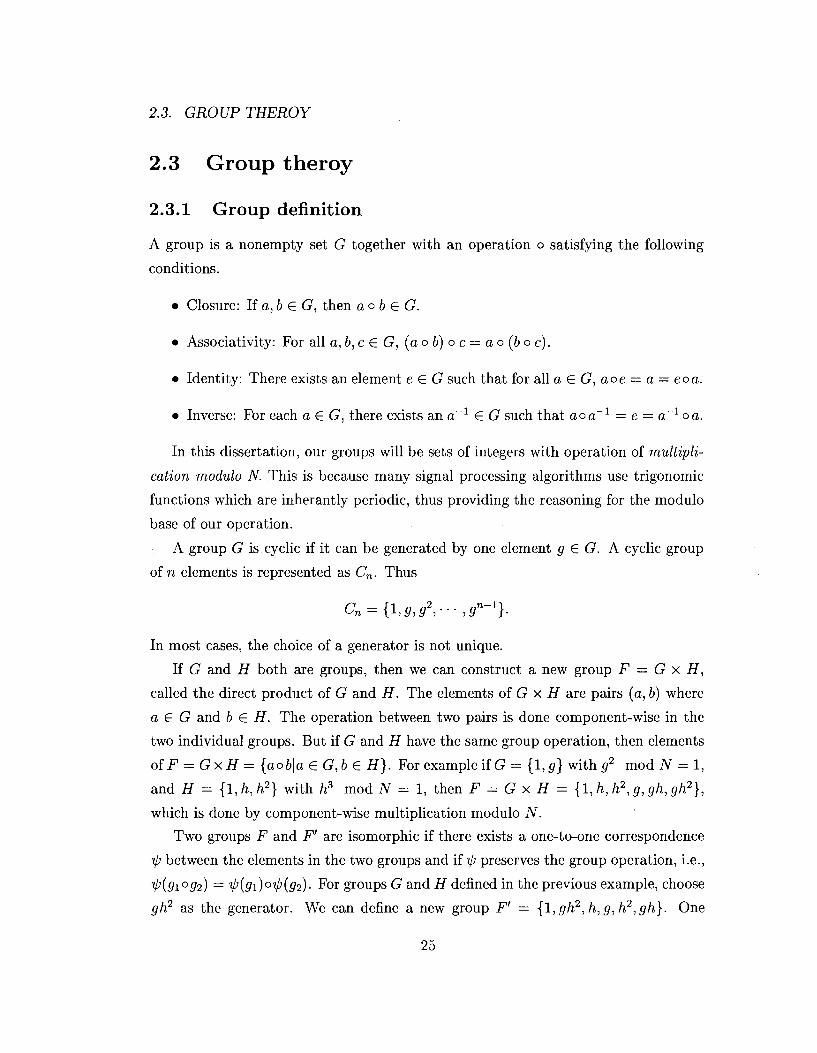
A group is a nonempty set G together with an operation o satisfying the following
conditions.
• Closure: If a, b E G, then a o b e G.
• Associativity: For all a, b, c € G, (a o b) o c = a o (6 o c).
• Identity: There exists an element e G G such that for all a € G, aoe = a = eoa.
• Inverse: For each a £ G: there exists an a~1 € G such that a o o - 1 = e = a~l oo.
In this dissertation, our groups will be sets of integers with operation of multipli
cation modulo N. This is because many signal processing algorithms use trigonomic
functions which are inherantly periodic, thus providing the reasoning for the modulo
base of our operation.
A group G is cyclic if it can be generated by one element g £ G. A cyclic group
of n elements is represented as Cn. Thus
Cn = {l,g,g2,~-,9n-1}-
In most cases, the choice of a generator is not unique.
If G and H both are groups, then we can construct a new group F — G x H,
called the direct product of G and H. The elements of G x H are pairs (a, 6) where
a G G and b € H. The operation between two pairs is done component-wise in the
two individual groups. But if G and H have the same group operation, then elements
o f F = G x t f = {aob\aeG,be H}. For example if G = {1, g} with g2 mod iV = 1,
and H = {l,h,h2} with h3 mod N = 1, then F = G x H = {l,h,h2,g,gh,gh2},
which is done by component-wise multiplication modulo N.
Two groups F and F' are isomorphic if there exists a one-to-one correspondence
ijj between the elements in the two groups and iff/' preserves the group operation, i.e.,
i>{gi°g2) = V,(5i)°V'(flr2)- For groups G and H defined in the previous example, choose
gh2 as the generator. We can define a new group F' = {l,gh2,h,g,h2,gh}. One
25
CHAPTER 2. ASIC METHODOLOGY AND MATHEMATICAL BACKGROUND
can verify that groups F and F' are isomorphic. Note that computations expressed
over one group can always be translated over to an equivalent group without extra
computational effort.
In an Abelian group, operation o is commutative, that is for all a,b G G, aob — boa.
Positive integers which are less than N and relatively prime to N, form an Abelian
group under the operation of multiplication modulo N. We will denote this group by
A(N). From the fundamental theorem of group theory, every finite Abelian group is
a product of cyclic groups. In particular, A(N) can be decomposed according to the
following rules.
• ^(rir2) = A{rr) x A(r2) when gcd(ri,r2)= 1.
• A(pn) = C(p_i)pn-i when p is an odd prime.
• A{2n) = C2 x C2n-2 when n > 3, A{A) = C2 and A(2) = {1}.
In addition, for a cyclic group,
• CTlT2 = CTl x CT2 when gcd (r1;r2)= 1.
2.3.2 Cyclic and Hankel matr ix products
Many signal processing algorithms rely heavily on matrix multiplication. This is
especially true in the time-frequency analysis of the signal. A two-dimensional kernel
matrix generally involves the time and frequency indices. We can reorder the indices
and transform the kernel (maybe in parts) to certain desirable forms. Using efficient
algorithms for these parts, one can then obtain efficient implementations for the DSP
applications. This section explains the desriable matrix forms we will use heavily in
this dissertation.
The most common matrix we use is a Hankel matrix. A general form of iV-point
26
2.3. GROUP THEROY
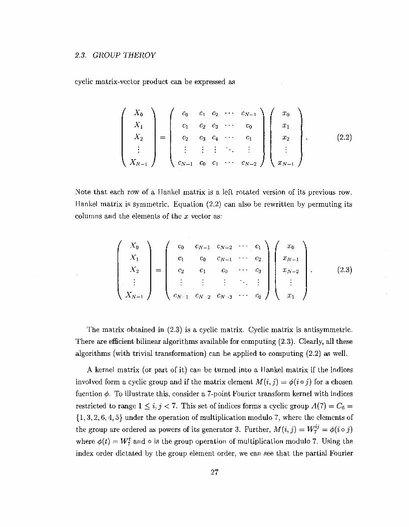
cyclic matrix-vector product can be expressed as
/ X0 \ x1
x2
I c0 cx c2
C\ C2 C3
c2 c3 c4
V XN_i J \ cN-i c0 ci
CAT. -A Co
Cl
/ XQ
XI
X2
CN-2 J \ XN-1 /
(2.2)
Note that each row of a Hankel matrix is a left rotated version of its previous row.
Hankel matrix is symmetric. Equation (2.2) can also be rewritten by permuting its
columns and the elements of the x vector as:
/ Xa \ Lo
x2
\ xN_, J
I Co CN-i CN-2
Ci C0 CN-i
C2 Ci C0
\ C T V - 1 CN-2 CN-3
C 1 \
c2
c3
/ XQ
XN-1
XN-2
Co / \ Xi )
(2.3)
The matrix obtained in (2.3) is a cyclic matrix. Cyclic matrix is antisymmetric.
There are efficient bilinear algorithms available for computing (2.3). Clearly, all these
algorithms (with trivial transformation) can be applied to computing (2.2) as well.
A kernel matrix (or part of it) can be turned into a Hankel matrix if the indices
involved form a cyclic group and if the matrix element M(i,j) = <f>(ioj) for a chosen
fucntion <j>. To illustrate this, consider a 7-point Fourier transform kernel with indices
restricted to range 1 < i,j < 7. This set of indices forms a cyclic group A(7) — Ce —
{1, 3, 2,6,4, 5} under the operation of multiplication modulo 7, where the elements of
the group are ordered as powers of its generator 3. Further, M(i,j) = W]3 — <fi(i°j)
where <f>(t) — W? and o is the group operation of multiplication modulo 7. Using the
index order dictated by the group element order, we can see that the partial Fourier
27
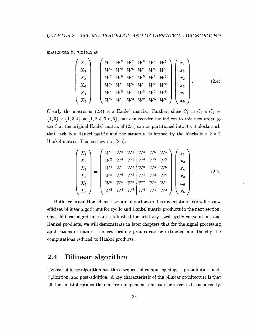
CHAPTER 2. ASIC METHODOLOGY AND MATHEMATICAL BACKGROUND
matrix can be written as
X3
x2 X,
x± x5 \A5J
( w1 w3 w2 w® w4 w5 \ w3 w2 w6 w4 w5 w1
w2 w6 w4 w5 w1 w3
w6 w4 w5 w1 w3 w2
W4 Wb Wl W3 W2 WG
w5 w1 w3 w2 w6 w4
fxx\ x3
X2
x6
\x, J
(2.4)
Clearly the matrix in (2.4) is a Hankel matrix. Further, since CQ = C2 x C3 =
{1,3} x {1,2,4} = {1,2,4,3,6,5}, one can reorder the indices to this new order to
see that the original Hankel matrix of (2.4) can be partitioned into 3 x 3 blocks such
that each is a Hankel matrix and the structure is formed by the blocks is a 2 x 2
Hankel matrix. This is shown in (2.5).
\
x2
x3
x6 \x5/
( wl w2
w2 w4
w4 w1
w3 ws
w6 w5
w5 w3
w4
wl
w2
w5
w3
w6
w3 w6 w5 \ w6 w5 w3
w5 w3 w6
w1 w2 w4
w2 w4 w1
W4 W1 W2 j
f Xl\ x2
Xi
x3
x6
\X5J
(2.5)
Both cyclic and Hankel matrices are important in this dissertation. We will review
efficient bilinear algorithms for cyclic and Hankel matrix products in the next section.
Once bilinear algorithms are established for arbitrary sized cyclic convolutions and
Hankel products, we will demonstrate in later chapters that for the signal processing
applications of interest, indices forming groups can be extracted and thereby the
computations reduced to Hankel products.
2.4 Bilinear algorithm
Typical bilinear algorithm has three sequential computing stages: pre-addition, mul
tiplication, and post-addition. A key characteristic of the bilinear architecture is that
all the multiplications therein are independent and can be executed concurrently.
28
2.4. BILINEAR ALGORITHM
Since there is only one multiplication along the critical data path, the structured
bilinear hardware has potential to achieve ultra-fast VLSI implementation.
Bilinear algorithms have been studied earlier by Rader [42] for prime length DFT
and by Winograd [61] for certain short composite length DFT. Recently bilinear al
gorithms have been proposed for more general length 2n DFT [55]. The process of
converting a transform to a bilinear algorithm consists of two steps. First, group
theory is used to identify convolution structures within the transform kernel matrix.
Typically one looks for cyclic and Hankel sub-matrices within the kernel. Using bi
linear algorithms for these cyclic and Hankel matrix-vector multiplications, a bilinear
algorithm is obtained for the complete transform.
2.4.1 Recursive decomposition
The basic building blocks for our targeted applications are the bilinear algorithms
for cyclic convolutions and Hankel products of prime power lengths. For small prime
lengths, these algorithms are well documented [3]. Bilinear algorithms for large prime
lengths can be derived as well [54]. A general cyclic matrix of any size can always be
decomposed into smaller cyclic matrices of relatively prime lengths. Similarly a large
size Hankel matrix can be decomposed into smaller Hankel matrices. In addition, a
cylic or Hankel matrix of prime power length can be decomposed into smaller cyclic
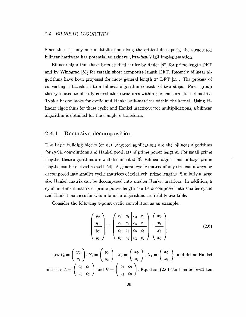
and Hankel matrices for whom bilinear algorithms are readily available.
Consider the following 4-point cyclic convolution as an example.
2/2
( C0 Ci
C\ C 2
c2 c3
\ c3 c0
C2 C3 \
C3 C0
Co C\
C\ C2 /
/ x0 \
X2 (2.6)
Let Y0 ' , ^ 1 = X0 x0
Xi ,X,
X2
X3
, and define Hankel
matrices A = [ \ and B — [ | . Equation (2.6) can then be rewritten c\ c2 c2 c0
29
CHAPTER 2. ASIC METHODOLOGY AND MATHEMATICAL BACKGROUND
as a 2-point block cyclic convolution as
A B \ ( X, \ (2.7)
Applying 2-point bilinear algorithm (Fig. 2.6) for cyclic convolution to (2.7), one
gets
Y0 = {(A + B)(X0 + X1) + (A-B){X0-X1))/2
*i = ( ( ^ + B)(X0 + X 1 ) - ( ^ - B ) ( X 0 - ^ i ) ) / 2 . (2.8)
The block coefficient matrices are:
A + B = I
A-B = (
c0 + c2 cx+cz \
c\ + c3 c0 + c2 J '
c0 - c2 ci - c3 Cl - C3 - ( C 0 - C 2 )
(2.9)
Therefore the block multiplication with (A + B) is again a 2-point cyclic matrix
multiplication requiring 2 multiplications and 4 additions in a bilinear algorithm.
The multiplication with (A — B) however, is a 2-point Hankel product and its bilinear
algorithm needs 3 multiplications and 3 additions. Putting together the blocks, the
complete bilinear algorithm shown in Fig. (2.7) is obtained. The net arithmetic
complexity of a bilinear algorithm for (2.6) is therefore 5 multiplications and 15
additions and the critical path delay is one multiplication and 4 additions.
In this dissertation, we employ this kind of recursive decomposition approach
repeatedly. A key aspect of the approach is that only a small number of bilinear algo
rithms are needed in order to obtain the solution to a much larger problem size. The
small number of required algorithm means more efficient design reuse for both soft
ware and hardware. When sizes are parameterized, it can reduce the overall code size
and shorten the design schedule since the verification effort is reduced substantially.
2 . 4 . 2 O r d e r o f c o m p u t a t i o n
When a larger bilinear algorithm is decomposed into two or more smaller algorithms,
it is important to determine the order of decomposition which provides the minimum
complexity. A bilinear algorithm can be characterized as a triplet (n, a, m), where n
30
2.4. BILINEAR ALGORITHM
(" C 0" C 1 + C 2 + C 3) / 2
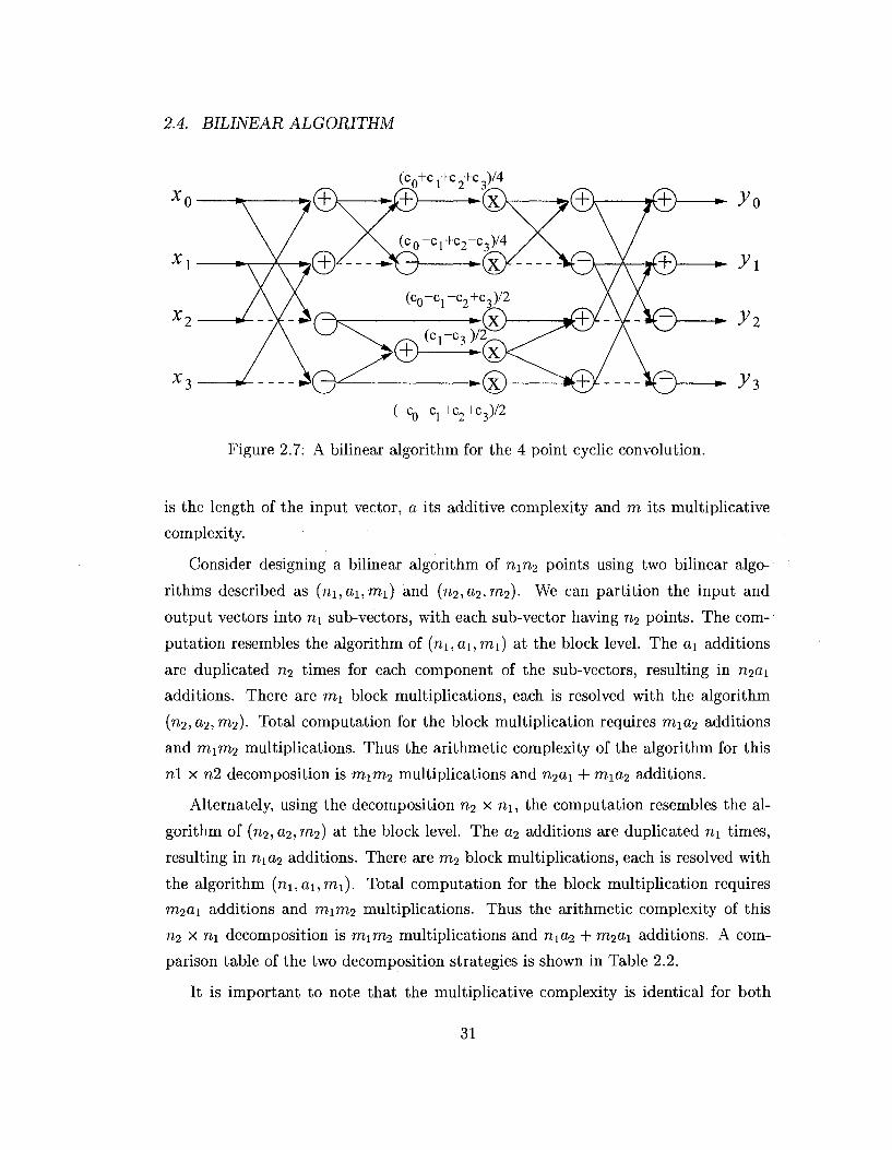
Figure 2.7: A bilinear algorithm for the 4 point cyclic convolution.
is the length of the input vector, a its additive complexity and m its multiplicative
complexity.
Consider designing a bilinear algorithm of nin2 points using two bilinear algo
rithms described as (ni,ai,mi) and (rz2, a2,m2). We can partition the input and
output vectors into n\ sub-vectors, with each sub-vector having n2 points. The com
putation resembles the algorithm of (ni,ai,mi) at the block level. The a\ additions
are duplicated n2 times for each component of the sub-vectors, resulting in n2«i
additions. There are mx block multiplications, each is resolved with the algorithm
(n2,a2,m2). Total computation for the block multiplication requires mia2 additions
and mim2 multiplications. Thus the arithmetic complexity of the algorithm for this
n\ x n2 decomposition is mim2 multiplications and n2ax + mia2 additions.
Alternately, using the decomposition n2 x rti, the computation resembles the al
gorithm of (ri2, 0,2,1712) at the block level. The a2 additions are duplicated n\ times,
resulting in nia2 additions. There are m2 block multiplications, each is resolved with
the algorithm (ni,ai,mi). Total computation for the block multiplication requires
m2ai additions and mim.2 multiplications. Thus the arithmetic complexity of this
n2 x n\ decomposition is mim2 multiplications and nia2 + m2ai additions. A com
parison table of the two decomposition strategies is shown in Table 2.2.
It is important to note that the multiplicative complexity is identical for both
31
CHAPTER 2. ASIC METHODOLOGY AND MATHEMATICAL BACKGROUND
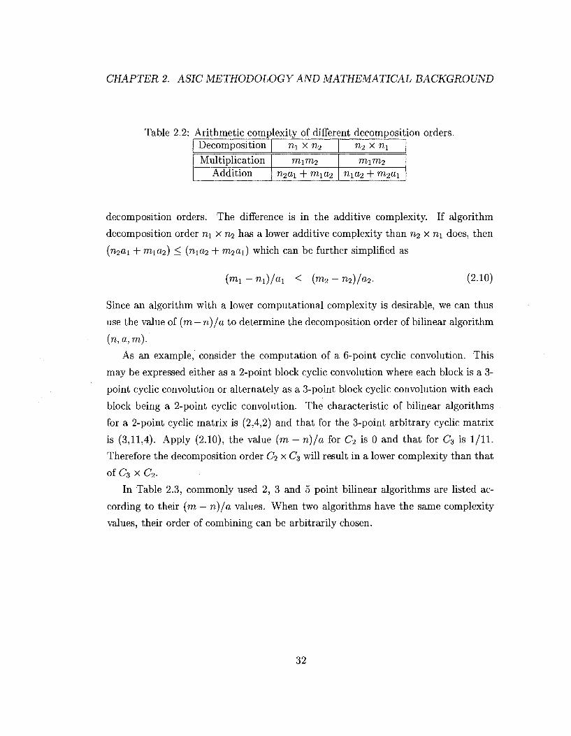
Table 2.2: Arithmetic complexity of different decomposition orders. Decomposition
Multiplication Addition
ni x n2
vn,\vn,2 n2a\ + m\a2
n2 x ni
m\m2
nxa2 + m2ai
decomposition orders. The difference is in the additive complexity. If algorithm
decomposition order n\ x n2 has a lower additive complexity than n2 x n\ does, then
{n2a\ + m,ia2) < (nia2 + m2a\) which can be further simplified as
(mi - n i ) /a i < (m2 - n2)/a2. (2-10)
Since an algorithm with a lower computational complexity is desirable, we can thus
use the value of (m — n)/a to determine the decomposition order of bilinear algorithm
(n, a,m).
As an example, consider the computation of a 6-point cyclic convolution. This
may be expressed either as a 2-point block cyclic convolution where each block is a 3-
point cyclic convolution or alternately as a 3-point block cyclic convolution with each
block being a 2-point cyclic convolution. The characteristic of bilinear algorithms
for a 2-point cyclic matrix is (2,4,2) and that for the 3-point arbitrary cyclic matrix
is (3,11,4). Apply (2.10), the value (m - n)/a for C2 is 0 and that for C$ is 1/11.
Therefore the decomposition order C2 x C3 will result in a lower complexity than that
of C3 x C2.
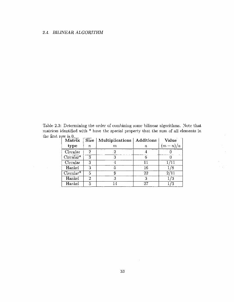
In Table 2.3, commonly used 2, 3 and 5 point bilinear algorithms are listed ac
cording to their (m — n)/a values. When two algorithms have the same complexity
values, their order of combining can be arbitrarily chosen.
32
2.4. BILINEAR ALGORITHM
Table 2.3: Determining the order of combining some bilinear algorithms. Note that matrices identified with * have the special property that the sum of all elements in the first row is 0.
Matrix type
Circular Circular* Circular Hankel
Circular* Hankel Hankel
Size n
2 3 3 3 5 2 5
Multiplications m
2 3 4 •5
9 3 14
Additions a
4 6 11 16 22 3
27
Value (m — n)/a
0 0
1/11 1/8
2/11 1/3 1/3
33
CHAPTER 2. ASIC METHODOLOGY AND MATHEMATICAL BACKGROUND
34
Chapter 3
Discrete Hartley transform
This chapter develops bilinear algorithms for the discrete Hartley transform (DHT)
of pn points for a prime p. Using a group theoretic approach, we show that the DHT
kernel matrix can be recursively transformed into cyclic and Hankel sub-matrices.
By using bilinear algorithms for cyclic convolution and Hankel product, one can
then obtain bilinear algorithms for the DHT. Bilinear algorithms ensure highest com
putational speeds in dedicated hardware. We have implemented in VLSI our new
algorithms of 2™ and 3" point DHTs as well as the ones available in literature. We
find that our algorithms have a speed advantage of 20% - 30% over others.
3.1 Background and prior work
The iV-point discrete Hartley transform (DHT) of sequence {x(i)}, is defined as [6]
N-l
X(k) = ^2x{i)cas{2irik/N), k = 0 , 1 , . . . , N - 1, (3.1) i=0
where cas(a) = cos (a) +sin(a) . The DHT is a real-valued transform with its forward
and inverse transforms sharing the same kernel (except for a scaling factor) and is
useful for obtaining convolutions of real sequences. It has also been used in many
applications in the fields of spectral analysis [57], error control coding [62], data
compression [64], and optics and microwave [6,7]. Further, it has been shown that fast
35
CHAPTER 3. DISCRETE HARTLEY TRANSFORM
Hartley transform (FHT) has the fastest realization of the DFT when implemented
across a variety of general purpose processor platforms [20].
Most of the algorithms for the DHT target von Neumann architecture. Since all
the operations in such general purpose computers are sequential, the performance of
these algorithms is evaluated by means of their arithmetic complexity and the number
of memory accesses [2,4,21,28,58]. However, the recent progress of VLSI technology
has now made it possible to develop cost effective dedicated Application Specific In
tegrated Circuits (ASIC) for signal processing applications. The ready availability of
low cost field programmable gate arrays (FPGA) has made such hardware solutions
practical even for low volume applications. Unfortunately, efficient algorithms devel
oped for general purpose computers such as the split-radix algorithm [2,4], separate a
2"-point DHT into n serial computation stages each involving multiplications. Thus,
if converted to hardware, the critical path of these algorithms involves several multi
plications one after the other. Fig. 3.1 shows a typical computational flow graph of a
2"-point DHT using a split-radix algorithm.
rotation re-order
Figure 3.1: Flow graph for Ref. [2] implementation of 2"-point DHT. Note that each rotation can also be implemented with 3 multiplciations and 3 additions. The index and the coefficients are: i',k' — 0,l,--- ,N/2 — 1; C(j) = cos(2ivj/N) and S(j) = sin(27rj/iV), where j = 0,1, • • • , N/4 - 1.
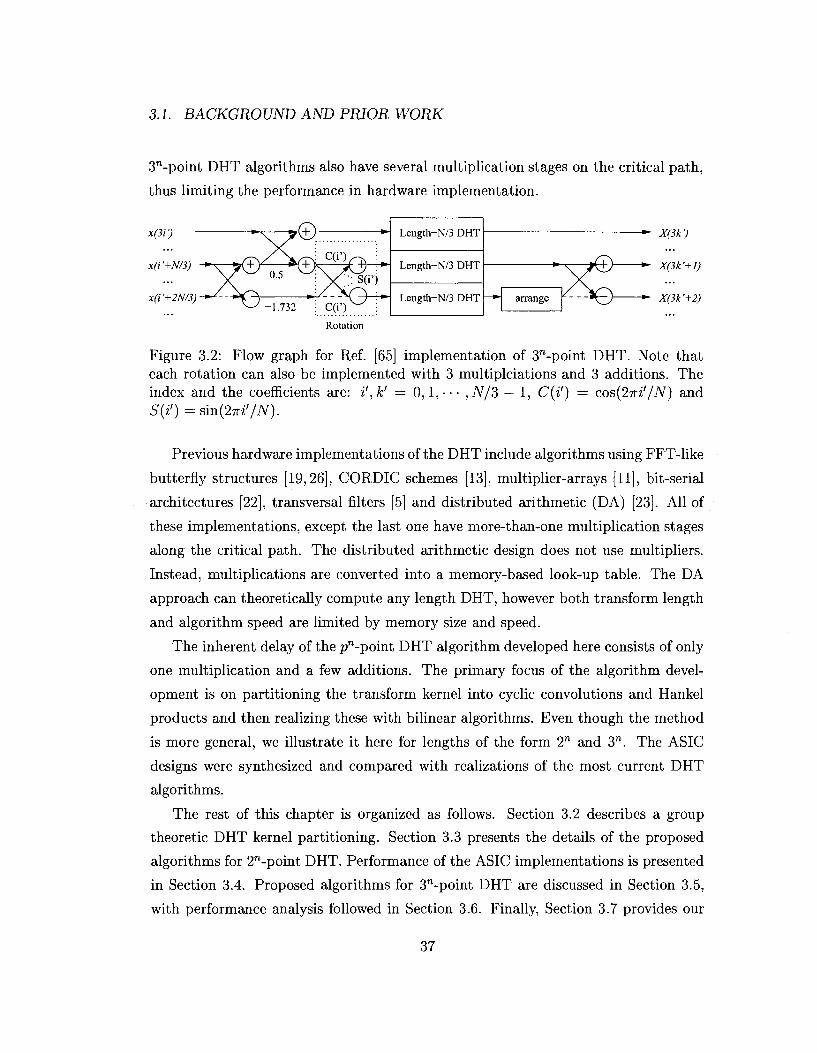
Split-radix algorithms have also been proposed for 3n-point DHT [1,29,65]. The
signal flow graph of a 3"-point DHT [65] is shown in Fig. 3.2. As can be seen from
the figure, these algorithms require additional computations to separate indices into
evenly divided three or nine bands. Hence these algorithms are quite different from
those of 2™-point DHT. However, similar to the algorithms for 2"-point DHT, these
36
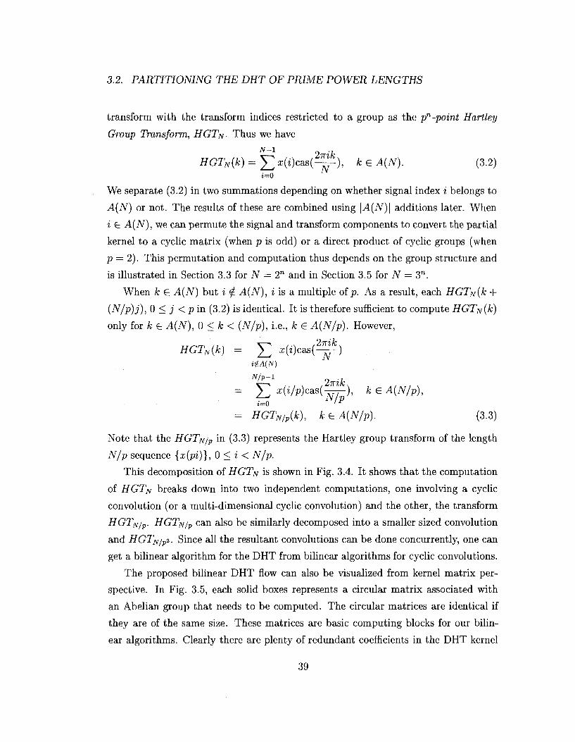
3.1. BACKGROUND AND PRIOR WORK
3n-point DHT algorithms also have several multiplication stages on the critical path,
thus limiting the performance in hardware implementation.
x(i'+2N/3)
Length-N/3 DHT
Length-N/3 DHT
Length-N/3 DHT arrange
X(3k')
X(3k'+1)
X(3k'+2)
Figure 3.2: Flow graph for Ref. [65] implementation of 3n-point DHT. Note that each rotation can also be implemented with 3 multiplciations and 3 additions. The index and the coefficients are: i',k' = 0,l,--- , iV/3 — 1, C(i') = cos(2-jri'/N) and S(i') = sm(2m'/N).
Previous hardware implementations of the DHT include algorithms using FFT-like
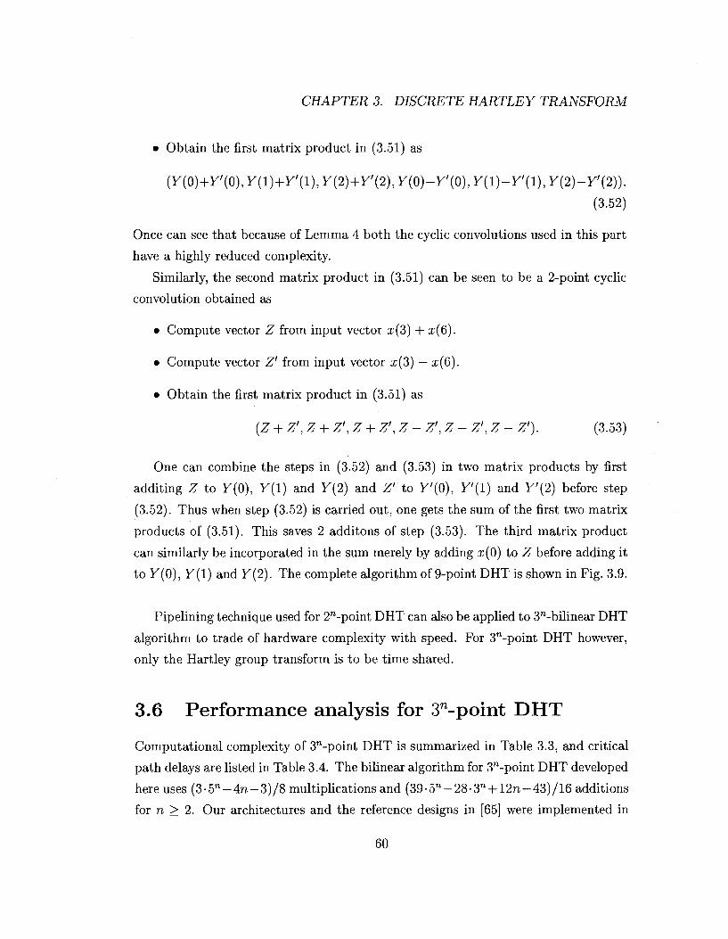
Once can see that because of Lemma 4 both the cyclic convolutions used in this part
have a highly reduced complexity.
Similarly, the second matrix product in (3.51) can be seen to be a 2-point cyclic
convolution obtained as
• Compute vector Z from input vector x(3) + x(6).
• Compute vector Z' from input vector x(3) — x(6).
• Obtain the first matrix product in (3.51) as
(Z + Z',Z + Z', Z + Z',Z-Z',Z- Z', Z - Z'). (3.53)
One can combine the steps in (3.52) and (3.53) in two matrix products by first
additing Z to Y(0), Y(l) and F(2) and Z' to F'(0), F ' ( l ) and Y'{2) before step
(3.52). Thus when step (3.52) is carried out, one gets the sum of the first two matrix
products of (3.51). This saves 2 additons of step (3.53). The third matrix product
can similarly be incorporated in the sum merely by adding x(0) to Z before adding it
to F(0), y ( l ) and F(2). The complete algorithm of 9-point DHT is shown in Fig. 3.9.
Pipelining technique used for 2n-point DHT can also be applied to 3n-bilinear DHT
algorithm to trade of hardware complexity with speed. For 3n-point DHT however,
only the Hartley group transform is to be time shared.
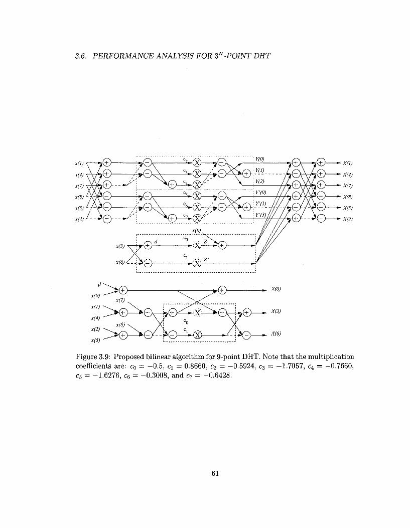
3.6 Performance analysis for 3n-point DHT
Computational complexity of 3"-point DHT is summarized in Table 3.3, and critical
path delays are listed in Table 3.4. The bilinear algorithm for 3n-point DHT developed
here uses ( 3 - 5 " - 4 n - 3 ) / 8 multiplications and (39-5 n -28-3 n + 12n-43) /16 additions
for n > 2. Our architectures and the reference designs in [65] were implemented in
60
3.6. PERFORMANCE ANALYSIS FOR 3N-POINT DHT
x(6)/_4£Q
X(0)
X(3)
X(6)
Figure 3.9: Proposed bilinear algorithm for 9-point DHT. Note that the multiplication coefficients are: c0 = -0.5, d = 0.8660, c2 = -0.5924, c3 = -1.7057, c4 = -0.7660, c5 = -1.6276, c6 = -0.3008, and c7 = -0.6428.
61
CHAPTER 3. DISCRETE HARTLEY TRANSFORM
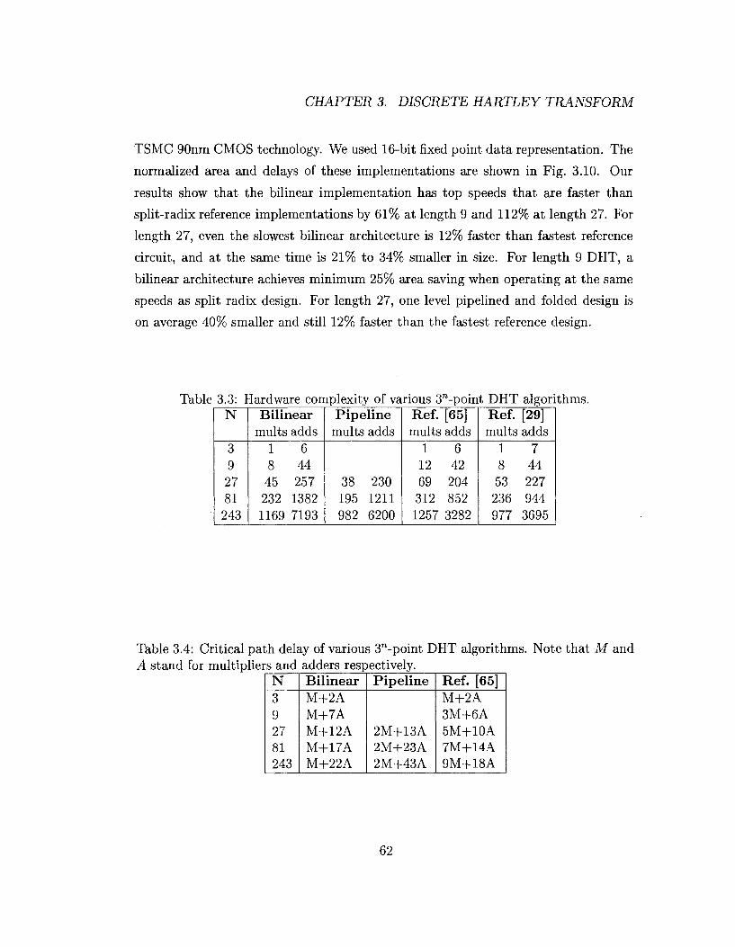
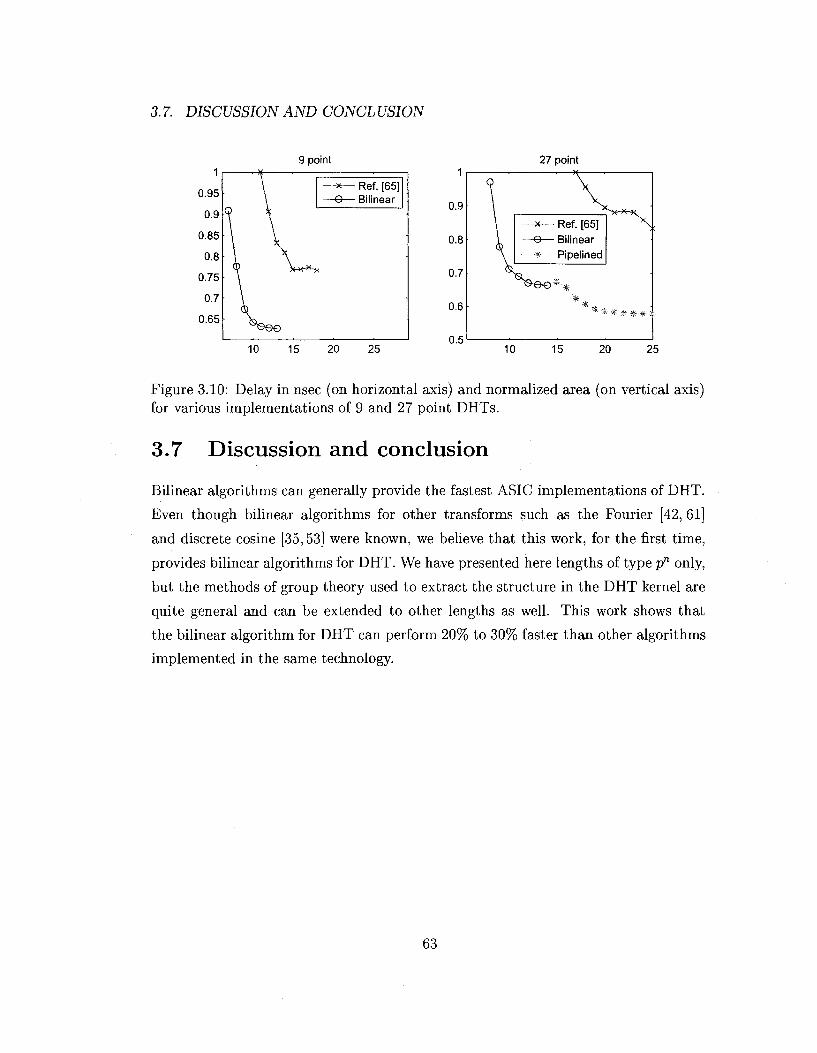
TSMC 90nm CMOS technology. We used 16-bit fixed point data representation. The
normalized area and delays of these implementations are shown in Fig. 3.10. Our
results show that the bilinear implementation has top speeds that are faster than
split-radix reference implementations by 61% at length 9 and 112% at length 27. For
length 27, even the slowest bilinear architecture is 12% faster than fastest reference
circuit, and at the same time is 21% to 34% smaller in size. For length 9 DHT, a
bilinear architecture achieves minimum 25% area saving when operating at the same
speeds as split radix design. For length 27, one level pipelined and folded design is
on average 40% smaller and still 12% faster than the fastest reference design.
Table 3.3: Hardware complexity of various 3"-point DHT algorithms. N
3 9 27 81 243
Bilinear mults adds
1 6 8 44
45 257 232 1382 1169 7193
Pipeline mults adds
38 230 195 1211 982 6200
Ref. [65] mults adds
1 6 12 42 69 204 312 852 1257 3282
Ref. [29] mults adds
1 7 8 44 53 227 236 944 977 3695
Table 3.4: Critical path delay of various 3"-point DHT algorithms. Note that M and A stand for multipliers and adders respectively.
N 3 9 27 81 243
Bilinear M+2A M+7A M+12A M+17A M+22A
Pipeline
2M+13A 2M+23A 2M+43A
Ref. [65] M+2A 3M+6A 5M+10A 7M+14A 9M+18A
62
3.7. DISCUSSION AND CONCL USION
9 point 27 point 1 , • • — x
0.9
0.8
0.7
0.6
0.5
- * — Ref. [65] - e — Bilinear » Pipelined
* * # * *
10 15 20 25
Figure 3.10: Delay in nsec (on horizontal axis) and normalized area (on vertical axis) for various implementations of 9 and 27 point DHTs.
3.7 Discussion and conclusion
Bilinear algorithms can generally provide the fastest ASIC implementations of DHT.
Even though bilinear algorithms for other transforms such as the Fourier [42, 61]
and discrete cosine [35,53] were known, we believe that this work, for the first time,
provides bilinear algorithms for DHT. We have presented here lengths of type pn only,
but the methods of group theory used to extract the structure in the DHT kernel are
quite general and can be extended to other lengths as well. This work shows that
the bilinear algorithm for DHT can perform 20% to 30% faster than other algorithms
implemented in the same technology.
63
CHAPTER 3. DISCRETE HARTLEY TRANSFORM
64
Chapter 4
Modified discrete cosine transform
Forward and inverse modified discrete cosine transforms (MDCT/IMDCT) are widely
used for subband coding in the analysis and synthesis filterbanks of time domain alias
ing cancellation (TDAC). Many international audio coding standards rely heavily on
fast algorithms for the MDCT/IMDCT. In this chapter we present hardware efficient
bilinear algorithms to compute MDCT/IMDCT of 2n and 4 • 3 n points. The algo
rithms for composite lengths have practical applications in MPEG-1/2 audio layer III
(MP3) encoding and decoding. It is known that the MDCT/IMDCT can be converted
to type-IV discrete cosine transforms (DCT-IV). Using group theory, our approach
decomposes DCT-IV transform kernel matrix into groups of cyclic and Hankel matri
ces. Bilinear algorithms are then applied to efficiently evaluate these groups. When
implemented in VLSI, our algorithms greatly improve the critical path delay as com
pared with the existing solutions. This is due to the fact that bilinear algorithms
employ only one multiplication along the critical path. For MP3 audio, we propose
three different versions of the unified hardware architectures for both the short and
long blocks, and the forward and inverse transforms.
4.1 Background and prior work
The forward and inverse modified discrete cosine transforms (MDCT/IMDCT) are
used as analysis and synthesis filter bank in transform/subband coding schemes, such
65
CHAPTER 4. MODIFIED DISCRETE COSINE TRANSFORM
as the time domain aliasing cancellation (TDAC) [41] and the modulated lapped
transform (MLT) [31]. The MDCT/IMDCT are basic computing elements in many
transform coding standards [38, 39]. Since the MDCT and IMDCT require inten
sive computations, fast and efficient algorithms for theses transforms is a key to the
realization of high quality audio and video compression schemes [50,51,63].
The iV-point modified discrete cosine transform (MDCT) of a sequence {x(i)} is
defined as
/ x ^ * fir(2i + l + %)(2k + l)\ N , x
X(*) = $ > ( 0 c o s M ^ M , * = 0 , 1 , . . . , — - 1 . (4.1)
Note the similarity between the kernel of the MDCT and that of the discrete cosine
transform (DCT). However unlike a DCT, MDCT converts N signal samples into
only N/2 transform samples.
There have been many fast algorithms proposed for the MDCT and its inverse,
IMDCT. Based on the symmetry of the transform matrix, Malvar [30] converts an N-
point MDCT into an iV/2-point type-IV discrete sine transform (DST-IV). Duhamel
et al. [18] compute the MDCT/IMDCT through the fast Fourier transform (FFT). An
A-point DCT is reduced to an A/4-point complex-valued FFT. Though the overall
arithmetic complexities between the two algorithms are similar, FFT algorithm has
the advantage of existing hardware realization [24]. In [12,14,36], the MDCT and
IMDCT are computed using recursive kernels. Recursive implementations require less
hardware at the expense of extending the critical path.
Unfortunately most MDCT algorithms are formulated for N = 2" and do not di
rectly apply to composite data lengths. Many existing applications of MDCT/IMDCT
however, use composite data lengths. For example, MPEG-1/2 layer III (MP3) audio
format specifies two frames consisting of 1152 and 384 data samples. These frames
are further partitioned into 32 subbands. A long block processes 36 data samples and
a short block 12 data samples. If implemented directly as in the ISO, the arithmetic
complexity of this composite A-point MDCT is A 2 / 2 multiplications and (A2 — N)/2
additions. Britanak and Rao [8,9] have designed efficient MDCT algorithms for MP3
audio. Their algorithms are based on Given's rotations. Depending on block sizes, 3
or 9 point DCT and DST modules are then used to obtain the results. For MDCT, the
66
4.1. BACKGROUND AND PRIOR WORK
DCT and DST used are of type-II. For IMDCT, they are of type-Ill. Their approach is
further refined by Nikolajevic and Fettweis [37], where the number of additions are re
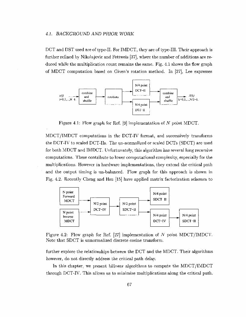
duced while the multiplication count remains the same. Fig. 4.1 shows the flow graph
of MDCT computation based on Given's rotation method. In [27], Lee expresses
.,N-1.
combine and
shuffle rotations
N/4 point
DCT-II
N/4 point
DST-II
combine and
shuffle k=0,l,
Figure 4.1: Flow graph for Ref. [9] implementation of N point MDCT.
MDCT/IMDCT computations in the DCT-IV format, and successively transforms
the DCT-IV to scaled DCT-IIs. The un-normalized or scaled DCTs (SDCT) are used
for both MDCT and IMDCT. Unfortunately, this algorithm has several long recursive
computations. These contribute to lower computational complexity, especially for the
multiplications. However in hardware implementations, they extend the critical path
and the output timing is un-balanced. Flow graph for this approach is shown in
Fig. 4.2. Recently Cheng and Hsu [15] have applied matrix factorization schemes to
N point Forward MDCT
N point Inverse MDCT
*
N/2 point
DCT-IV
N/2 point
SDCT-II
N/4 point
SDCT-II
N/4 point
DCT-IV
N/4 point
SDCT-II
Figure 4.2: Flow graph for Ref. [27] implementation of iV point MDCT/IMDCT. Note that SDCT is unnormalized discrete cosine transform.
further explore the relationships between the DCT and the MDCT. Their algorithms
however, do not directly address the critical path delay.
In this chapter, we present bilinear algorithms to compute the MDCT/IMDCT
through DCT-IV. This allows us to minimize multiplications along the critical path.
67
CHAPTER 4. MODIFIED DISCRETE COSINE TRANSFORM
Using group theory, we decompose the transform kernel into cyclic and Hankel ma
trix products. Bilinear algorithms are then used to efficiently evaluate these matrix
products. We show that when implemented in VLSI with fixed-point arithmetic, our
approach significantly reduces the critical path delay.
The rest of this chapter is organized as follows. Section 4.2 reviews the steps
of transforming MDCT/IMDCT to DCT-IV. In Section 4.3, bilinear algorithms for
2"-point MDCT/IMDCT are presented. Section 4.4 develops bilinear algorithms
for MDCT/IMDCT with composite lengths of 4 • 3". In particular, a 12-point
MDCT/IMDCT is used for MP3 short block processing as a 6-point DCT-IV. The
MP3 long block of 36-point MDCT/IMDCT is computed by an 18-point DCT-IV.
For all DCT-IV algorithms, we discuss group structures, arithmetic complexities, and
critical path delays that are associated with the bilinear algorithm implementation.
In particular for the MP3 application, we explore three different versions of the uni
fied hardware architecture for both the short and long blocks, and the forward and
inverse transforms. Section 4.5 provides the conclusion of this chapter.
4.2 Transformation from TV-point M D C T / I M D C T
to 7V/2-point DCT-IV
As pointed out earlier, an TV-point MDCT uses N signal samples to create N/2
transform samples. The first step in the computation of MDCT therefore involves
converting this N x N/2 kernel into a kernel of a known square transform. It is
known that an TV-point MDCT/IMDCT can be transformed into an iV/2-point type-
IV DCTs [12,27,30,31]. Our derivation here closely follows that of [27].
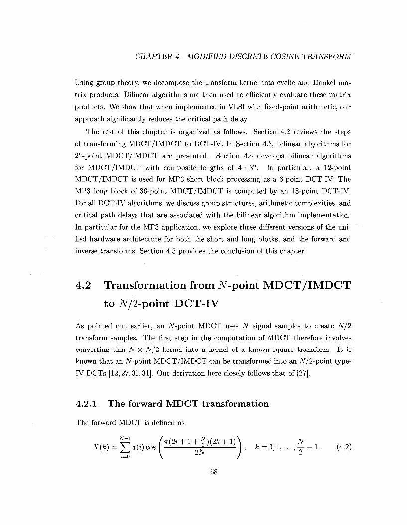
4.2.1 The forward M D C T transformation
The forward MDCT is defined as
68
4.2. TRANSFORMATION FROM N-POINT MDCT/IMDCT TO N/2-P0INT DCT-IV
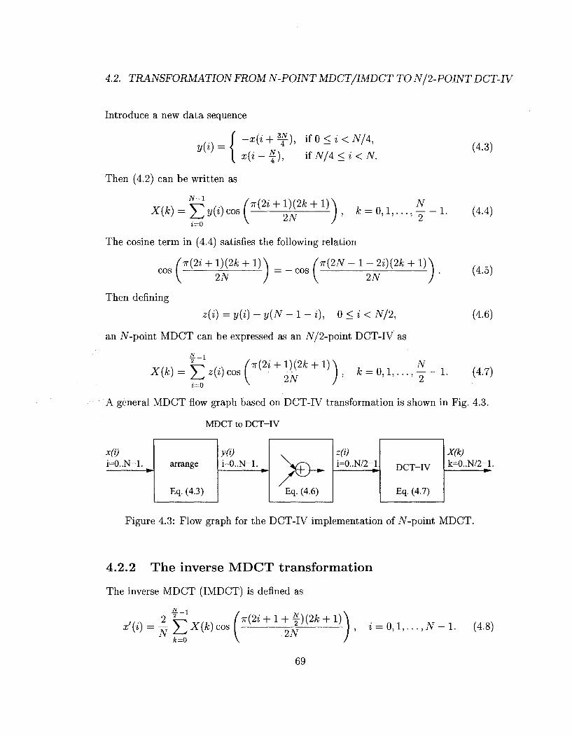
Introduce a new data sequence
l s (* - f )> HN/4<i<N.
Then (4.2) can be written as
N-l x(k)= Yl y(^cos
i=0
7r(2i + l)(2k + l)\ N — I, * - U , l , . . . , - - l .
The cosine term in (4.4) satisfies the following relation
ir(2i + l)(2k + l)\ _ _ (K{2N - 1 - 2i)(2k + 1)
2N J "~ \ 2N
Then defining
z(i) = y(i) - y(N -1-i), 0<i< N/2,
an iV-point MDCT can be expressed as an Af/2-point DCT-IV as
-l K 2
X(k) = Y J z(i) cos i=0
7r{2i + l)(2k + 1)\ . _ . N
2N , fc = Q , 1 , . . . , - - 1 .
(4.3)
(4.4)
(4.5)
(4.6)
(4.7)
A general MDCT flow graph based on DCT-IV transformation is shown in Fig. 4.3.
MDCT to DCT-IV
x(i) i=0..N-l. arrange
Eq. (4.3)
y(i) i=0..N-l.
*+ Eq. (4.6)
z(i) i=0..N/2-l DCT-IV
Eq. (4.7)
X(k) k=0..N/2-1.
Figure 4.3: Flow graph for the DCT-IV implementation of iV-point MDCT.
4.2.2 The inverse M D C T transformation
The inverse MDCT (IMDCT) is defined as
*'« = N E X W cos k=0
7r(2z + l + f)(2A; + l)
2N
69
i = 0 , l , . . . , J V - l . (4.8)
CHAPTER 4. MODIFIED DISCRETE COSINE TRANSFORM
To obtain the IMDCT, first compute the iV/2-point type-IV DCT of X as
*'« = ̂ E*w cos 8 = 0
7r(2i + l)(2ft + l) N i = 0 , l , . . . , - - l . (4.9)
Applying the symmetry property (4.5), and defining a new data sequence
f z'(i), if 0<i< N/2-1, y (i) — s
{ -z'(N -1-i), if N/2<i< N,
the IMDCT output x'(i) can then be recovered as
(4.10)
x'{i) M + n i f 0 < i < ^ - l , -y'(i-^), i f f < t < J V - l .
(4.11)
An IMDCT flow graph based on DCT-IV transformation is shown in Fig. 4.4.
DCT-IV to IMDCT
X(k) k=0..N/2-l. DCT-IV
Eq. (4.9)
z'(i) i=0..N/2-l Expand
Eq. (4.10)
y'0) i=0..N-l. Re-order
Eq. (4.11)
x'(i) i=0..N-l.
Figure 4.4: Flow graph for the DCT-IV implementation of N point IMDCT.
4.2.3 The advantage of DCT-IV transformation
The DCT-IV transformation has significant implication on implementations, espe
cially for hardware. It is clear from Figs. 4.3 and 4.4 that a common DCT-IV module
can be shared for both the forward and inverse transforms. Unified hardware archi
tecture for the MDCT and IMDCT is shown in Fig. 4.5. Note that we purposedly
scale the data sample to 2N points so that the core computation module becomes an
Appoint DCT-IV.
A key challenge to ASIC implementation is the requirement on the number of
input and output (10) pins. From a package point of view, the reduction of pad 10
size has not kept pace with the development of transistor technology. From a macro
70
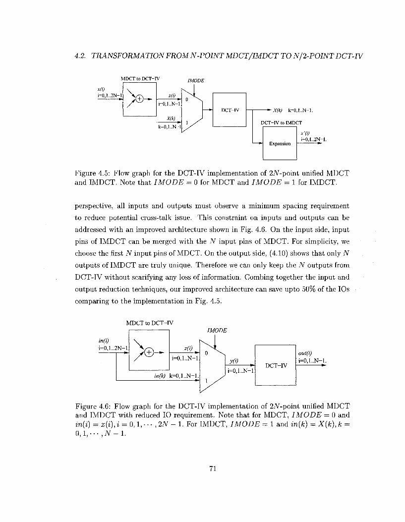
4.2. TRANSFORMATION FROM N-POINT MDCT/IMDCT TO N/2-P0INT DCT-IV
1..N-1.
i=0,1..2N-l. ^-
Figure 4.5: Flow graph for the DCT-IV implementation of 2iV-point unified MDCT and IMDCT. Note that IMODE = 0 for MDCT and IMODE = 1 for IMDCT.
perspective, all inputs and outputs must observe a minimum spacing requirement
to reduce potential cross-talk issue. This constraint on inputs and outputs can be
addressed with an improved architecture shown in Fig. 4.6. On the input side, input
pins of IMDCT can be merged with the N input pins of MDCT. For simplicity, we
choose the first N input pins of MDCT. On the output side, (4.10) shows that only N
outputs of IMDCT are truly unique. Therefore we can only keep the N outputs from
DCT-IV without scarifying any loss of information. Combing together the input and
output reduction techniques, our improved architecture can save upto 50% of the IOs
comparing to the implementation in Fig. 4.5.
in(i)
i=0,1..2N-l
Figure 4.6: Flow graph for the DCT-IV implementation of 2JV-point unified MDCT and IMDCT with reduced 10 requirement. Note that for MDCT, IMODE = 0 and in(i) = x{i), i = 0,1, • • • , 2N - 1. For IMDCT, IMODE = 1 and in{k) = X(k), k = 0 , 1 , . - - , J V - 1 .
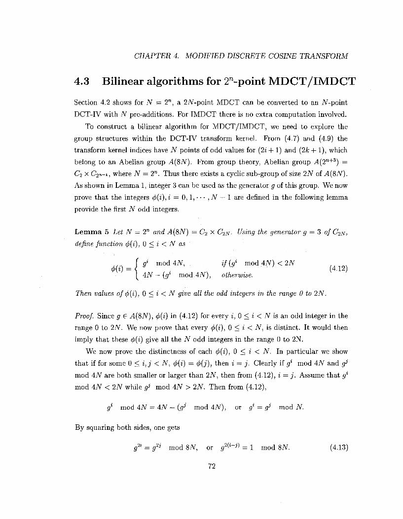
4.3 Bilinear algorithms for 2n-point M D C T / I M D C T
Section 4.2 shows for N — 2n, a 2iV-point MDCT can be converted to an iV-point
DCT-IV with JV pre-additions. For IMDCT there is no extra computation involved.
To construct a bilinear algorithm for MDCT/IMDCT, we need to explore the
group structures within the DCT-IV transform kernel. From (4.7) and (4.9) the
transform kernel indices have iV points of odd values for (2i + 1) and (2k + 1), which
belong to an Abelian group A(8N). From group theory, Abelian group A(2n+3) =
C2 x C*2n+i, where N — 2n. Thus there exists a cyclic sub-group of size 2N of A(8N).
As shown in Lemma 1, integer 3 can be used as the generator g of this group. We now
prove that the integers <p(i), i — 0,1,- • • ,N — 1 are defined in the following lemma
provide the first N odd integers.
L e m m a 5 Let N = 2n and A(8N) = Ci x C2N- Using the generator g = 3 of C2N,
define function 4>(i), 0 < i < N as
i gi mod AN, if (gi mod AN) <2N , <j>[%) = { y . ' J Ky ' (4.12)
[ AN — (gl mod 4AQ, otherwise.
Then values of <p(i), 0 < i < N give all the odd integers in the range 0 to 2N.
Proof. Since g €E A(8N), <fi(i) in (4.12) for every i, 0 < i < N is an odd integer in the
range 0 to 2N. We now prove that every c/>(i), 0 < i < N, is distinct. It would then
imply that these <p(i) give all the N odd integers in the range 0 to 2N.
We now prove the distinctness of each (p(i), 0 < i < N. In particular we show
that if for some 0 < i, j < N, (f)(i) = (/)(j), then i — j . Clearly if gl mod 4Af and gi
mod 4A^ are both smaller or larger than 2AT, then from (4.12), i = j . Assume that g%
mod AN < 2N while gj mod 4JV > 2N. Then from (4.12),
g{ mod AN = 4N - (gj mod AN), or gi = gj mod N.
By squaring both sides, one gets
g2i = g2j mod 8N, or g2{i'j) = 1 mod 8N. (4.13)
72
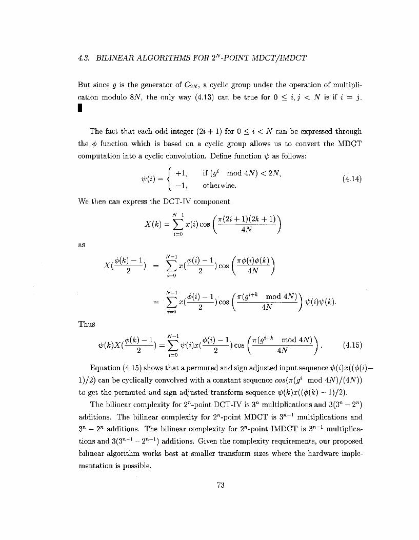
4.3. BILINEAR ALGORITHMS FOR 2N-POINT MDCT/IMDCT
But since g is the generator of CW, a cyclic group under the operation of multipli
cation modulo 8iV, the only way (4.13) can be true for 0 < i,j < N is if % = j .
I
The fact that each odd integer (2i + 1) for 0 < i < N can be expressed through
the (j) function which is based on a cyclic group allows us to convert the MDCT
computation into a cyclic convolution. Define function ip as follows:
0 W f + l . if to* mod4A0<2AT, ( ^ y —1, otherwise.
We then can express the DCT-IV component
N-l
as
i=0 ^ '
x{m-1) _ N£xim^±)caj«-mm\ 4N J
Thus
i=0
W)Xir^\ ) = E ^W^(^H—)cos I — 4jy ) • (4-15)
Equation (4.15) shows that a permuted and sign adjusted input sequence il>(i)x(((f)(i)-
l)/2) can be cyclically convolved with a constant sequence cos(ir(gt mod 4N)/(4N))
to get the permuted and sign adjusted transform sequence ip(k)x({(f){k) — l)/2).
The bilinear complexity for 2"-point DCT-IV is 3n multiplications and 3(3" - 2")
additions. The bilinear complexity for 2n-point MDCT is 3"_ 1 multiplications and
3" - 2" additions. The bilinear complexity for 2n-point IMDCT is 3 n _ 1 multiplica
tions and 3(3"_1 — 2n_1) additions. Given the complexity requirements, our proposed
bilinear algorithm works best at smaller transform sizes where the hardware imple
mentation is possible.
73
CHAPTER 4. MODIFIED DISCRETE COSINE TRANSFORM
We illustrate the above through an 8-point DCT-IV which is employed in a 16-
point MDCT. Let x(i) and X(i), 0 < i < 8, denote the input and output samples of
the DCT. In this case, g being 3, the values of <j>(i) for i = 0 through 7 are given by
{1,3, 9,5,15,13, 7,11}. The consecutive values of ip(i) are {1,1,1, —1, —1,1, —1,1}.
Using a shorthand notation^ for a value of cos(-KpjAN) and J? be a value of — cos(irp/4N)
with N = 8, we can describe the transform matrix for 8 point DCT-IV as
X(0)\
X(l)
X(4)
-X(2)
-X(7)
X(6)
-X(3)
X{h) )
( 1
3
9
5
15
13
7
V 1 1
3 9 5
9 5 15
5 15 13
15 13 7
13 7 11
7 11 T
11 T 3
T 3 9
T5
13
7
11
T 3
9
5
13
7
11
T
3
9
5
15
7 11 \̂
11 T
T 3
3 9
9 5
5 15
15 13
13 7 )
( x(0)
x(l)
x(4)
-x{2)
-x(7)
x(6)
-x(3)
{ x(5)
A Hankel matrix product is derived and efficient bilinear algorithm can then be
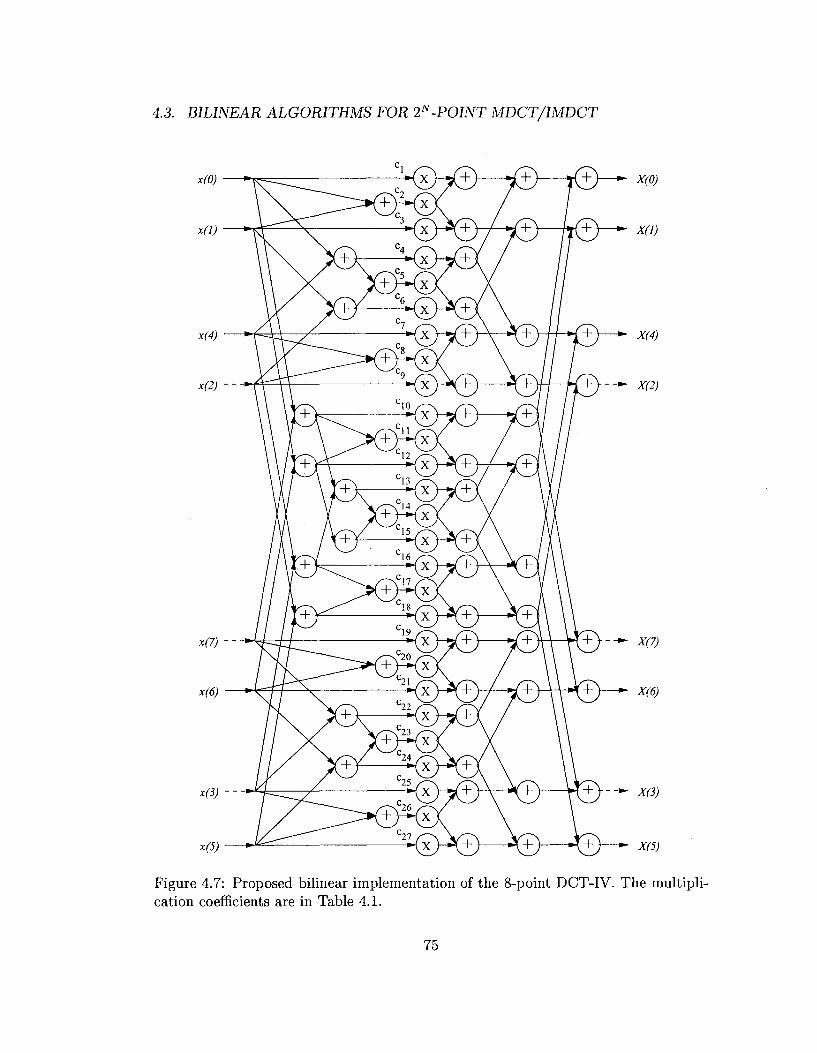
applied to compute the transform. This algorithm is shown in Fig. 4.7. Inidividual
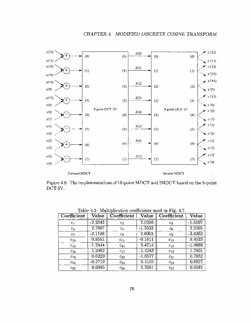
architecture for 16-point MDCT and IMDCT based on this 8-point DCT is shown
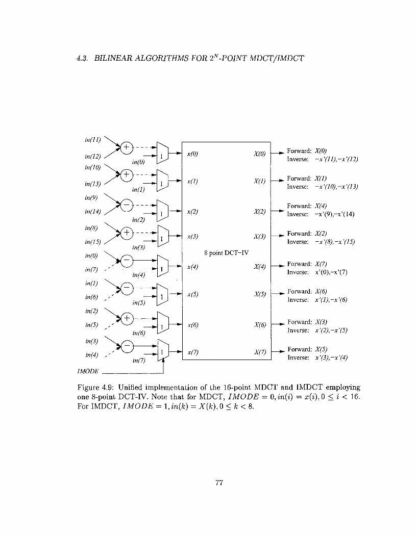
in Fig. 4.8, whereas a unified architecture is shown in Fig. 4.9. A solid line means a
transfer function of 1, a dashed line means a transfer function of —1. The multipli
cation coefficients are listed in Table 4.1.
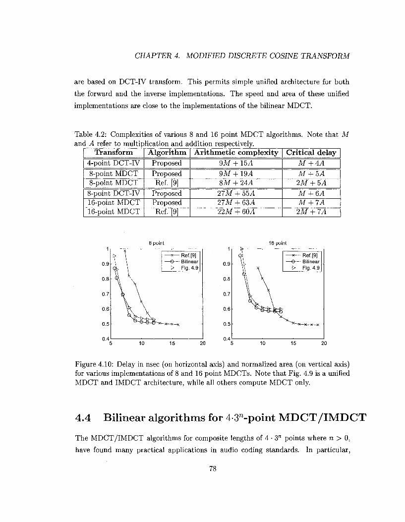
For lengths 8 and 16, our proposed algorithms for MDCT are compared to [9]
which offers a regular structure based on Given's Rotation. The complexities and
critical path delays are shown in Table 4.2. The algorithms are implemented in 16-
bit fixed arithmetic with TSMC 90nm CMOS standard cell library. The normalized
area and speed comparison of the resultant circuits is shown in Fig. 4.10. For 8-point
MDCT, the top speed of the proposed bilinear implementation is 30% higher than
that of [9]. For 16-point MDCT, our speed advantage is over 44%. In fact, the top
speed of 16-point bilinear implementation is even 15% faster than that of the 8-point
implementation of [9]. Given the same speed, the area for 8-point bilinear circuits
can be as much as 32% smaller than that of [9]. For 16-point, the proposed circuit
can be as much as 26% smaller. In addition, the MDCT bilinear implementations
74
4.3. BILINEAR ALGORITHMS FOR 2N-P0INT MDCT/IMDCT
(+)—*- x(i)
+y— x(4)
X(2)
X(0)
X(7)
X(6)
X(3)
X(5)
Figure 4.7: Proposed bilinear implementation of the 8-point DCT-IV. The multiplication coefficients are in Table 4.1.
75
CHAPTER 4. MODIFIED DISCRETE COSINE TRANSFORM
x(12) '
x(ll)
x(13)
x(10)
x(14)
x(9)
x(15)
x(8)
x(0)
x(7)
x(l)
x(6) ,
x(2)
x(5)
x(3)
x(4)
r+\---+\
+ \ — ~\
+ > — - J
+\ — *\
(0)
(1)
(2)
(3)
(5)
(6)
(7)
(0)
(1)
(2)
(3)
8 point DCT-IV
(4) (4)
(5)
(6)
(7)
X(0)
X(l)
X(2)
X(3)
X(4)
X(5)
X(6)
X(7)
(0)
(1)
(2)
(3)
(5)
(6)
(7)
(0) V
(1)
(2)
(3)
8 point DCT-IV
(4) (4)
(5)
(6)
(7)
,* x'(12)
^x'(U)
.* x'(13)
^ x ' ( 1 0 )
,* "'(14)
X x'(9)
." x'(15)
^-KxX8)
S x'(0)
X x-(l)
X x'(2)
-^x'(5)
X x'(3)
X x'(4)
Forward MDCT Inverse MDCT
Figure 4.8: The implementations of 16-point MDCT and IMDCT based on the 8-point DCT-IV.
Table 4.1: Mu Coefficient
C\
c4
c?
ClO
Cl3
Cl6
Cl9
C22
C25
Value -2.3342 2.7607
-3.1108 0.8561
-1.2444 1.2062 0.6220
-0.2719 0.6985
tiplication coei Coefficient
c2
c5
c8
Cll
c14
Cl7
C20
C23
C26
Scients used in Fig. 4.7. Value 2.0200
-1.3533 2.6005
-0.1811 0.4714
-1.4283 -1.6577 0.4105 0.2561
Coefficient c3
C6
C9
Cl2
Cl5
Cl8
C21
C24
C27
Value -1.5097 2.2505
-3.6363 0.4033
-1.4666 1.7891 0.7032 0.6827 0.0581
76
4.3. BILINEAR ALGORITHMS FOR 2N-POINT MDCT/IMDCT
in(ll)
in(12)
in(10)
in(13)
in(9)
in(14)
in(8)
in(15)
in(0)
in(7) -
in(l)
in (6)
in(2)
in(5)
in (3)
in(4)
IMODE
'+} —-H in(0)
in(l)
in(2)
+ > — •
in(3)
in(4)
in(5)
+ in(6)
in(7)
x(0)
x(l)
x(2)
x(3)
X(0)
X(l)
X(2)
X(3)
8 point DCT-IV
x(4) X(4)
x(5)
x(6)
x(7)
X(5)
X(6)
X(7)
Forward: X(0) Inverse: — x '(11), —x '(12)
_^ Forward: X(l) Inverse: —x '(10), —x '(13)
Forward: X(4) ~*~ Inverse: -x'(9),-x'(14)
», Forward: X(2) Inverse: —x '(8), —x '(15)
Forward: X(7) Inverse: x'(0),-x'(7)
Forward: X(6) Inverse: x'(l),-x'(6)
_^ Forward: X(3) Inverse: x'(2),-x'(5)
_^ Forward: X(5) Inverse: x'(3),-x'(4)
Figure 4.9: Unified implementation of the 16-point MDCT and IMDCT employing one 8-point DCT-IV. Note that for MDCT, IMODE = Q,in(i) = x(i),0 < i < 16. For IMDCT, IMODE = l,in(k) =X(k),0<k<8.
77
CHAPTER 4. MODIFIED DISCRETE COSINE TRANSFORM
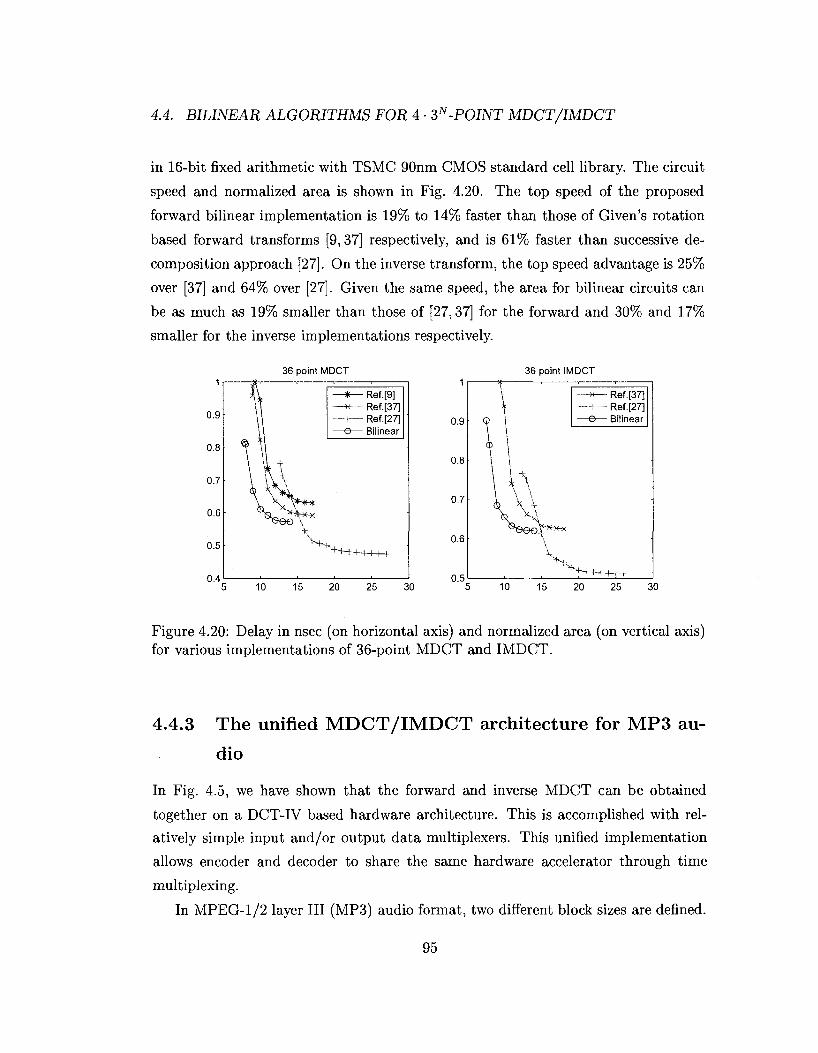
are based on DCT-IV transform. This permits simple unified architecture for both
the forward and the inverse implementations. The speed and area of these unified
implementations are close to the implementations of the bilinear MDCT.
Table 4.2: Complexities of various 8 and 16 point MDCT algorithms. Note that M and A refer to multiplication and addition respectively.
Critical delay M + 4A M + 5A 2M + 5A M + 6A M + 7A 2M + 7A
1
0.9
0.8
0.7
0.6
0.5
0.4
Figure 4.10: Delay in nsec (on horizontal axis) and normalized area (on vertical axis) for various implementations of 8 and 16 point MDCTs. Note that Fig. 4.9 is a unified MDCT and IMDCT architecture, while all others compute MDCT only.
4.4 Bilinear algorithms for 4-3n-point M D C T / I M D C T
The MDCT/IMDCT algorithms for composite lengths of 4 • 3" points where n > 0,
have found many practical applications in audio coding standards. In particular,
78
8 point 16 point
• *— Ref. [9] B— Bilinear -E>— Fig. 4.9
10 15 20
4.4. BILINEAR ALGORITHMS FOR 4 • 3N-POINT MDCT/IMDCT
12-point MDCT/IMDCT is used for the short block and 36-point MDCT/IMDCT is
used for the long block of MPEG-1/2 layer III (MP3) audio processing.
The algorithm for 4 • 3"-point MDCT can be designed following an approach
similar to the one in Section 4.2, i.e., a 2iV-point MDCT is first converted to an
iV-point DCT-IV as
X W = | > W c o s ( * ( a + ^ f + 1 ) ) , * = 0,1 J V - 1 . (4.17)
An iV-point IMDCT is computed directly from an iV-point DCT-IV to obtain one
half of the outputs. The other half is redundant and can be obtained with trivial sign
changes.
As discussed in Section 4.2, the MDCT of any even length can be computed via
a DCT-IV of half the length. Let N = 2 • 3" where n > 0. We will use the symbol
Xn to indicate a DCT-IV of length 2 • 3 n . Consider the group A(8N) = {0 < i <
8N | gcd(i, 8N) = 1}. The proposed computation shown in Fig. 4.11 uses transform
division of DCT-IV kernel matrix based on A(8N). For MDCT, it is a frequency
division scheme; for IMDCT, a time division scheme.
+» X(k) 2k+l £A(8N) and 0=<k<N.
+»X(k) 2k+l ftA(8N) and 0<k<N.
Figure 4.11: Flow graph for 2 • 3"-point bilinear DCT-IV.
Consider first the computation of Xn(k), where (2k + 1) ^ A(8N) , i.e. (2k +1) is
a multiple of 3. In this case, it can be shown that the multiplication coefficients for
79
Cosine Group Transform CGT„,
Pre-Addition
N/3-1 y(i)=^jX(i)-x(2N/3-i-l)-x(2N/3+i)
i=0 DCT-IV of length N/3
CHAPTER 4. MODIFIED DISCRETE COSINE TRANSFORM
x(i), x(2N/3 — i — 1) and x(2N/3 + i) are related. In particular,
-7r(2z + l)(2A: + l ) ^ _ _ fir(2(2N/3 - * - 1) + l)(2fc + 1) C O B I I — C<Oo
Figure 4.21: Proposed bilinear implementation of the unified 12 and 36 point MDCT and IMDCT (architecture A).
99
CHAPTER 4. MODIFIED DISCRETE COSINE TRANSFORM
Table 4.9: 12 and 36 point MDCT and IMDCT input mapping for unified architecture B. Note that xA and xB refer to the two 6-point blocks whose MDCT is computed concurrently. Similarly XA and XB represent two independent 6-point transform blocks whose IMDCT is computed concurrently.
4.4. BILINEAR ALGORITHMS FOR 4 • 3N-POINT MDCT/IMDCT
Table 4.10: 12 and 36 point MDCT and IMDCT output mapping for unified architecture B. Note that XA and XB refer to MDCTs of 6-point sequences xA and xB
respectively and are computed concurrently. Similarly x'A and x'B refer to IMDCTs of 6-point transforms XA and XB respectively and are computed concurrently.
O u t p u t
out(0) out(l) out (2) out(3) out(4) out(5) out(6) out (7) out(8) out(9)
out(10) out ( l l ) out(12) out(13) out(14) out(15) out(16) out (17)
MDCTm
X(0) X(l) X(2) X(3) X(4) X(5) X(6) X(7) X(8) X(9)
X(10) X( l l ) X(12) X(13) X(14) X(15) X(16) X(17)
(A,B) with bilinear 36-point MDCT and [9,37], and separately compared pipelined
architecture with a low complexity MDCT [27]. The fast unified architectures A and
B are 9% faster than that of [37] and 13% faster than that of [9] at top speed. At
higher speeds, the proposed designs can be more than 27% smaller. The pipelined
architecture is 26% faster than [27] at the top speed and 19% smaller if the speed is the
same. The three proposed unified architectures can process not only the forward and
inverse transforms, but also the short and long blocks in MP3 application, whereas
the compared reference designs can only compute forward MDCT for the long block.
For architecture B and pipelined architecture, two short blocks are processed in one
clock cycle.
106
4.4. BILINEAR ALGORITHMS FOR 4 • 3N-POINT MDCT/IMDCT
Table 4.13: Complexities of unified 12 and 36 point MDCT and IMDCT architectures for MP3 application. Note that M and A refer to multiplication and addition respectively.
Figure 4.24: Delay in nsec (on horizontal axis) and normalized area (on vertical axis) for unified 12 and 36 point MDCT and IMDCT architectures (A, B and pipeline), with comparison to the 36-point MDCT architectures in literature.
107
CHAPTER 4. MODIFIED DISCRETE COSINE TRANSFORM
4.5 Discussion and conclusion
Forward and inverse modified discrete cosine transforms (MDCT/IMDCT) are widely-
used for subband coding in the analysis and synthesis filterbanks of time domain alias
ing cancellation (TDAC). Many international audio coding standards rely heavily on
fast algorithms for the MDCT/IMDCT. In this chapter we have presented hardware
efficient bilinear algorithms to compute MDCT/IMDCT of 2" and 4 • 3n points. The
algorithms for composite lengths have practical applications in MP3 audio encoding
and decoding. It is known that the MDCT/IMDCT can be converted to type-IV
discrete cosine transforms (DCT-IV). Using group theory, our approach decomposes
DCT-IV transform kernel matrix into groups of cyclic and Hanke product matrices.
Bilinear algorithms are then applied to efficiently evaluate these groups. When im
plemented in VLSI, bilinear algorithms have improved the critical path delays over
existing solutions. For MPEG-1/2 layer III (MP3) audio, we propose three different
versions of unified hardware architectures for both the short and long blocks and the
forward and inverse transforms.
108
Chapter 5
Modulated complex lapped
transform
This chapter presents a new algorithm for the modulated complex lapped transform
(MCLT) with a sine window. It is shown that by merging the window with the main
computation, both the real and the imaginary parts of the MCLT with 2N inputs
can be obtained from two iV-point discrete cosine transforms (DCT) of appropriate
inputs. The resultant algorithm is computationally very efficient. The value of N can
be in general, an even number. When iV is a power of 2, the proposed algorithm uses
only N log N + 2 multiplications, with none of those being outside the DCT blocks.
5.1 Background and prior work
The modulated complex lapped transform (MCLT) is structured as a cosine- and
sine-modulated filter bank that maps overlapping blocks of a real-valued signal into
blocks of complex-valued transform coefficients [33]. It is a special form of a two
times oversampled discrete Fourier transform (DFT) filter bank to perform frequency
decomposition. Since the reconstruction formula of the MCLT is not unique, the
MCLT allows more flexible implementations of audio enhancement and encoding sys
tems than the DFT. Recent MCLT applications include acoustic echo cancellation [33]
109
CHAPTER 5. MODULATED COMPLEX LAPPED TRANSFORM
and audio watermarking [34] by using the phase information from the imaginary co
efficients.
The JV-point MCLT of a 2iV-point input sequence {x(n)} is defined as [33]
2 A T - 1
y(k) = Yl ^ n ' k ) - ^ ( n ' *)1 ^W- A; = 0 ,1 , . . . , iV - 1, (5.1)
where the real and imaginary parts of the MCLT kernel are defined as
Mn,*) = ^h{n)sm(^±i±§^±2)iy (5.2)
Function h(n) in (5.2) is the window function. The most common choice for h(n) is
the sine window specified as
M „ ) = - s i n ( < ^ ) , (5.3)
which is used in many applications such as MPEG-1 and MPEG-2 since it permits a
perfect reconstruction [31,41].
The real part of MCLT is the forward/direct modulated lapped transform (MLT)
[31], which is used to implement transform coding in video and audio compression
applications [46]. The MLT has also been referred to as time domain echo cancellation
(TDAC) [41] and cosine modulated filter banks [52]. The calculation of the MLT
involves scaling the input with a window function and then using a modified discrete
cosine transform (MDCT). Existing fast MDCT algorithms are either FFT-based or
DCT-based with pre- and post- permutations [10,15,18]. Computational efficiency
of the MLT can be improved by combining the window function with the MDCT
[18,24,32,45].
The original sequence {x(n)} can be recovered from MCLT by using either its real
or the imaginary part, or both [34]. If only the real part is used, the inverse transform
is the same as the inverse MLT (IMLT) which has been studied in detail [32]. Here we
focus on fast algorithm for the forward/direct MCLT where both real and imaginary
parts are required.
110
5.1. BACKGROUND AND PRIOR WORK
As a complex extension of the MLT, the MCLT shares many fast algorithms with
the MLT. Malvar has shown that the real part of MCLT with arbitrary window
function can be obtained from a discrete cosine transform (DCT) of type IV and
the imaginary, from a discrete sine transform (DST) of type IV [33] . However, the
computational complexity is affected by applying the window function to the input
before using the DCT or the DST. Later, FFT-based MCLT algorithms have been
developed that merge a sine window [34,49] with the main computation for improved
computational efficiency. Fig. 5.1 shows a patented computational flow using a FFT-
based algorithm. Another recently proposed MCLT algorithm applicable to arbitrary
2N real inputs 2N point FFT N+l complex rotation N complex coefficients complex outputs
c(0) - ^ ^ ^
x(0) *- u(0)
x(l) - u(l)
u(2)
u(N-l)
x(2N-l) *• u(N)
Figure 5.1: Flow graph for Ref. [34] implementation of the MCLT. Note that c(k) = W8(2k + l)W4N(k).
but symmetric window uses two DCTs to compute the real and imaginary parts
of the MCLT separately [17]. However, this algorithm employs permutation stages
with non-constant multiplications outside the main computation module limiting its
efficiency. In addition, this algorithm involves coefficient division, which could have
numerical instability when implemented in fixed-point precision for large transform
lengths. Flow graph of this algorithm is shown in Fig. 5.2.
In this chapter, we introduce a new MCLT algorithm with lower computational
complexity than other algorithms available today. We use a sine window and merge
its computation with the main computational modules. Our algorithm for 2N input
y(N-l)
111
CHAPTER 5. MODULATED COMPLEX LAPPED TRANSFORM
x(N-3)
x(N-2)
x(N-l)
Figure 5.2: Flow graph for Ref. [17] implementation of the MCLT. Note that c(i) — h(N — 1 — i)/h{i) and d(i) is a constant for a sine window. Each circle respresents an addition.
MCLT is based on the evenly stacked modified discrete cosine transform (Cjf) and
evenly stacked modified discrete sine transform (S^). The iV-point evenly stacked
MDCT and MDST are, respectively, denned as [41]:
Cf
°JV/2
i V - 1
o,
cos ^(2n + l + ^)k 0<k<N-l,
(5.4)
si cE ^0
2JV-1
= 2~] x(n)sm
n=0
0.
^(2n + l + y)A; 1 < k < N,
(5.5)
We show that 2iV-point C^ and S^ may be computed from two iV-point DCTs of
appropriately folded input sequences. On the other hand, the real and complex parts
of the MCLT can be obtained by adding the outputs of scaled C^ and Sjf with at
most two extra multiplications..
112
5.2. PROPOSED ALGORITHM
5.2 Proposed algorithm
We now show that both the real and the imaginary parts of MCLT may be obtained
from two iV-point DCT. However, unlike the iV-point DCT, the input sequence of
an MCLT has 2iV points. For mathematical convenience, we use two intermediate
transforms ADCT and ADST with 2N input and N + 1 output points defined as:
ADCT(k) = ^ = = 2 ] T cos (*k{2nw+N)) *(n), 0 < k < N, (5.6) 71=0
2N-1
ADST(k) = -L= J2 s in (^^N + N)) "(")• 0<*<7V. (5.7)
It is clear from (5.4) and (5.6) that ADCT is equivalent to a 2iV-point Cf scaled
by a constant of \/(2y/~N). Similarly, from (5.5) and (5.7), ADST is equivalent to a
2iV-point Sj? scaled by the same constant.
One can show that transforms ADCT and ADST (and equivalently Cf? and Sf?)
are related to DCT. To convert ADCT into an iV-point DCT, note that in the ADCT
computation of (5.6), the sequence components x(n + 3N/2) and x(3N/2 — n — 1) for
0 < n < N/2 — 1 multiply with the same cosine term cos(7rA;(2n + l)/(2JV)). Similarly,
the components x(n — N/2) and x(3N/2 — n — 1) for N/2 < n < N also multiply
with this same cosine term, cos(7rA;(2n + 1)/{2N)). Further, as n goes over the stated
ranges, the x component indices span the entire range of the input sequence from 0
to 2N — 1. To take advantage of this, define a sequence {xc(ri}} as:
f x{n + 3iV/2) + x(3N/2 - n - 1), if 0 < n < JV/2, , , xAn) = < (5.8)
{ x(n-N/2)+x(3N/2-n-l), if N/2 < n< N.
It is then obvious that
ADCT{k) = Jj= J2 cos ( 7 r M 22 ^ + 1 ) ) xe(n), 0 < k < N. (5.9)
Thus for 0 < k < N — 1, the ADCT of the sequence {x(n)} is the same as the
iV-point DCT (type II) of the sequence {xc(n)} except for a constant multiplication
factor 1/(2VN). These ADCT outputs can therefore be computed using any available
113
CHAPTER 5. MODULATED COMPLEX LAPPED TRANSFORM
DCT algorithms [25,43] without incurring additional computational penalty except
may be of one multiplication. Further, (5.9) also shows that
ADCT{N) = 0. (5.10)
Transform ADST can also be related to DCT in a similar way. In the definition
(5.7) of ADST, sequence components x(n + 3N/2) and -x(3N/2 - n - 1) when
0 < n < N/2 as well as x{n - N/2) and -x{3N/2 - n - 1) when N/2 < n < N all
multiply with the same sine term sin(7rfc(2? + 1)/(2JV)). Again, the indices of these
four x terms span the entire input index range, 0 to 2iV — 1, when n goes over the
specified ranges. To take advantage of this, define the sequence {xs(n)} as
, , f x(n + 3N/2) - x(3N/2 - n - 1), if 0 < n < N/2, xs{n) = < (5.11)
\x(n- N/2) - x{3N/2 - n - 1), if N/2 < n < N.
One can then see that
ADST(k) = -±= Y, s i n (1Tk{22N+l)) ^ ( " ) . 0 < ^ < iV. (5.12)
Equation (5.12) shows that except for the scaling factor l/(2\/N), transform
ADST(k), 1 < k < N, is the A^-point DST of type II and can be obtained using
any available algorithm for DST. But since we are already using the DCT for ADCT
computation, we prefer to use the same for the ADST computation as well. For this,
we employ an approach similar to that of [56]. Define a new sequence {xs(n)} as