42
SUBMITTED TO IEEE TRANSACTIONS ON INFORMATION THEORY 100
Binary Intersymbol Interference Channels:
Gallager Codes, Density Evolution and Code
Performance Bounds
Aleksandar Kav�ci�c, Xiao Ma and Michael Mitzenmacher
The material in this manuscript will be presented in part at the International Symposium on Information Theory,
Washington, DC, June 24-29, 2001.
The authors are with the Division of Engineering and Applied Sciences, Harvard University, Cambridge, MA.
This work was supported by the National Science Foundation under Grant No. CCR-9904458 and by the National
Storage Industry Consortium.
February 22, 2001 DRAFT
SUBMITTED TO IEEE TRANSACTIONS ON INFORMATION THEORY 101
Abstract
We study the limits of performance of Gallager codes (low-density parity-check codes) over binary
linear intersymbol interference (ISI) channels with additive Gaussian noise. Using the graph representa-
tions of the channel, the code and the sum-product message-passing detector/decoder, we prove two error
concentration theorems. Our proofs expand on previous work by handling complications introduced by
the channel memory. We circumvent these problems by considering not just linear Gallager codes but
also their cosets and by distinguishing between di�erent types of message ow neighborhoods depending
on the actual transmitted symbols. We compute the noise tolerance threshold using a suitably developed
density evolution algorithm and verify by simulation that the thresholds represent accurate predictions of
the performance of the sum-product algorithm for �nite (but large) block lengths. We also demonstrate
that for high rates the thresholds are very close to the theoretical limit of performance for Gallager codes
over ISI channels. If C denotes the capacity of a binary ISI channel and if Ci:i:d: denotes the maximal
achievable mutual information rate when the channel inputs are independent identically distributed (i.i.d.)
binary random variables (Ci:i:d: � C), we prove that the maximum information rate achievable by the
sum-product decoder of a Gallager (coset) code is upper-bounded by Ci:i:d:. The last topic investigated is
the performance limit of the decoder if the trellis portion of the sum-product algorithm is executed only
once; this demonstrates the potential for trading o� the computational requirements and the performance
of the decoder.
Keywords
intersymbol interference channel, channel capacity, i.i.d. capacity, BCJR-once bound, low-density
parity-check codes, Gallager codes, density evolution, sum-product algorithm, turbo equalization.
I. Introduction
If continuous channel inputs are allowed, the capacity of discrete-time intersymbol in-
terference (ISI) channels with additive Gaussian noise (AWGN) can be computed using
the water-�lling theorem [1], [2]. In many applications, the physics of the channel do not
allow continuous input alphabets. A prime example of a two-level (binary) intersymbol
interference channel is the saturation magnetic recording channel, because the magneti-
zation domains can have only two stable positions [3]. Other examples include digital
communication channels where the input alphabet is con�ned to a �nite set [4].
The computation of the capacity of discrete-time ISI channels with a �nite number
of allowed signaling levels is an open problem. In the past, the strategy has been to
February 22, 2001 DRAFT
SUBMITTED TO IEEE TRANSACTIONS ON INFORMATION THEORY 102
obtain numeric [5] and analytic [6], [7] bounds on the capacity. Very often authors have
concentrated on obtaining bounds on the maximum achievable information rate when the
inputs are independent and identically distributed (i.i.d.) { the so-called i.i.d. capacity [6],
[7]. Recently, a method for evaluating the i.i.d. capacity using the forward recursion
of the sum-product (BCJR/Baum-Welch) algorithm has been proposed by Arnold and
Loeliger [8]. This marks the �rst exact result involving a channel capacity of a discrete-
time ISI channel with binary inputs. The remaining issue is to devise codes that will
achieve the capacity (or at least the i.i.d. capacity).
The ability to achieve (near) channel capacity has recently been numerically demon-
strated for various memoryless [9], [10] channels using Gallager codes, also known as
low-density parity-check (LDPC) codes [11]. The theory of Gallager codes has vastly ben-
e�tted from the notion of codes on graphs �rst introduced by Tanner [12] and further
expanded into a unifying theory of codes on graphs by Wiberg et.al. [13] and Forney [14].
MacKay [15], [16] showed that there exist Gallager codes that outperform turbo codes [17].
A major breakthrough was the construction of irregular Gallager codes [18], and the de-
velopment of a method to analyze them for erasure channels [9], [19]. These methods were
adapted to memoryless channels with continuous output alphabets (additive white Gaus-
sian noise channels, Laplace channels, etc.) by Richardson and Urbanke [20], who also
coined the term \density evolution" for a tool to analyze the asymptotic performance of
Gallager and turbo codes over these channels [21]. The usefulness of the tool was demon-
strated by using it to optimize codes whose performance is proven to get very close to the
capacity, culminating in a remarkable 0.0045 dB distance from the capacity of the additive
white Gaussian noise (AWGN) channel reported by Chung et. al. [22].
In this paper, we focus on developing the density evolution method for channels with
binary inputs and ISI memory. The computed thresholds are used for lower-bounding the
capacity, as well as for upper-bounding the average code performance. The main topics of
this paper are: 1) concentration theorems for Gallager codes and the sum-product message-
passing decoder over binary ISI channels, 2) a density evolution method for computing the
thresholds of \zero-error" performance over these channels, 3) theorems establishing that
the asymptotic performance of Gallager codes using the sum-product algorithm is upper
February 22, 2001 DRAFT
SUBMITTED TO IEEE TRANSACTIONS ON INFORMATION THEORY 103
bounded by the i.i.d. capacity, and 4) the computation of the BJCR-once bound, which is
the limit of \zero-error" performance of the sum-product algorithms if the trellis portion
of the algorithm is executed only once.
The paper is organized as follows. In Section II, we describe the channel model, intro-
duce the various capacity de�nitions, and brie y describe the sum-product decoder [23].
In Section III, we introduce the necessary notation for handling the analysis of Gallager
codes for channels with memory and prove two key concentration theorems. Section IV
is devoted to describing the density evolution algorithm for channels with ISI memory.
In Section V, computed thresholds are shown for regular Gallager codes. Section V also
presents a theorem regarding the limit of achievable code rates using binary linear codes.
In this section we also develop the notion of the BCJR-once bound, which has a practical
implication, namely, it is the limit of performance of the sum-product algorithm if the
trellis portion of the algorithm is executed only once. This provides a concrete example
of how we can trade o� the computational load (by doing the expensive BCJR step only
once) with the decoding performance. Section VI concludes the paper.
Basic notation: Matrices are denoted with boldface uppercase letters (e.g., H). Col-
umn vectors are denoted by underlined characters. Random variables (vectors) are typ-
ically denoted by uppercase characters, while their realizations are denoted by lowercase
characters (e.g., a random vector W has a realization w). The superscript T denotes
matrix and vector transposition. If a column vector is s = [s1; s2; : : : ; sn]T, then a sub-
vector collecting entries si; si+1; : : : ; sj is denoted by sji = [si; si+1; : : : ; sj]T. The notation
Pr (event1) denotes the probability of event1, while Pr (event1jevent2) denotes the prob-
ability of event1 given that event2 occurred. The probability mass functions of discrete
random variables will be denoted with the symbol \Pr", e.g., the probability mass function
of a discrete random vector X evaluated at x will be denoted by Pr (X = x), i.e., it is the
probability that X takes the value x. The probability density function of a continuous
random variable will be denoted by the symbol \f". For example, the probability density
function of a continuous random vector Z evaluated at the point z will be denoted by
fZ (z).
February 22, 2001 DRAFT
SUBMITTED TO IEEE TRANSACTIONS ON INFORMATION THEORY 104
II. The Channel, Gallager Codes and Decoding
A. Channel model, graph representation and capacity
Assume that we have a real1 discrete-time intersymbol interference (ISI) channel of �nite
length I, characterized by the channel response polynomial h(D) = h0 + h1D + : : : hIDI ,
where hi 2 R. The input xt to the discrete-time channel at time t 2 Z is a realization of
a random variable Xt drawn from a �nite alphabet X � R. The output of the channel yt
is a realization of a random variable Yt drawn from the alphabet Y = R. The channel's
probabilistic law is captured by the equation
Yt =IXi=0
hiXt�i +Nt; (1)
where Nt is a zero-mean additive white Gaussian noise (AWGN) sequence with variance
E [N2t ] = �2 whose realizations are nt 2 R. In the sequel, we shall assume that the input
alphabet is binary X = f�1; 1g.
The channel in (1) is conveniently represented by a trellis [24], or equivalently, by a
graph where for each variable Xt there is a single trellis node [13], [14]. De�ne the state at
time t as the vector that collects the input variables Xt�I+1 through Xt, i.e,, Qt= X t
t�I+1.
The realization qtof the random vector Q
tcan take one of 2I values. With this notation,
we can factor the function
Pr�Xn
1 = xn1 jYn1 = yn
1; Q
0= q
0
�fY n
1 jQ0
�yn1jQ
0= q
0
�=
nYt=1
F�xt; yt; qt�1; qt
�; (2)
where each factor is
F�xt; yt; qt�1; qt
�= fYtjXt;Q
t�1
�ytjxt; qt�1
�Pr�Qt= q
tjQ
t�1 = qt�1
�: (3)
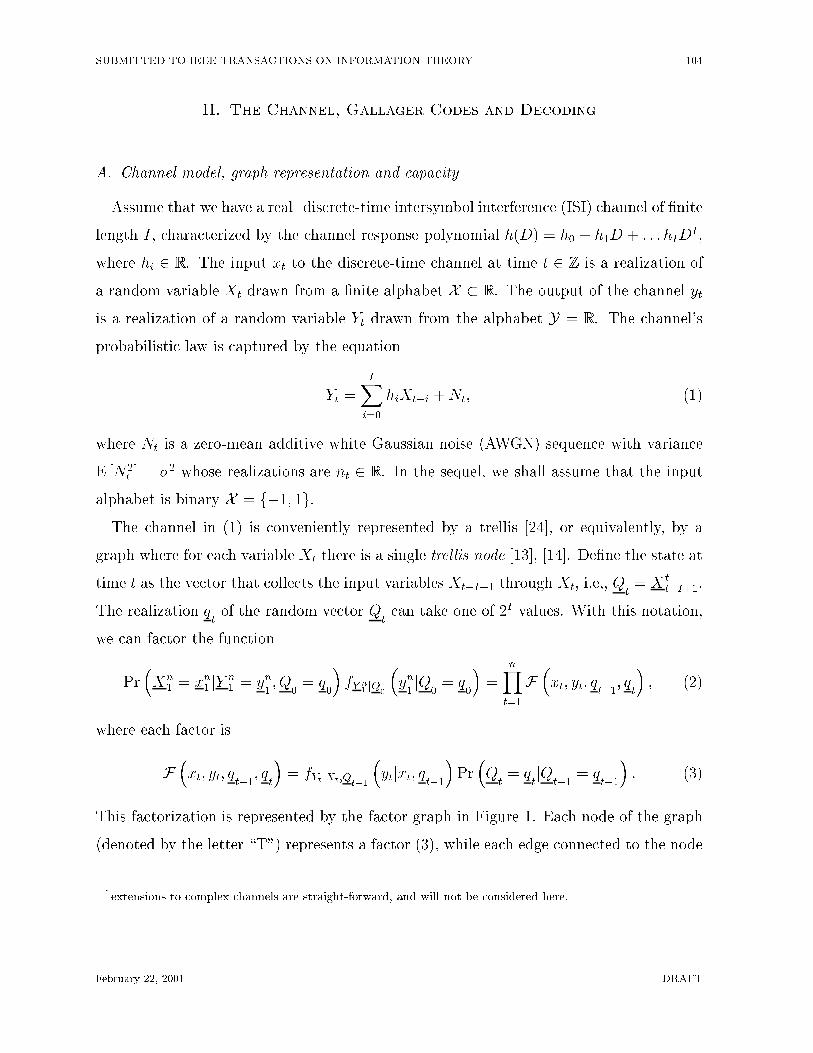
This factorization is represented by the factor graph in Figure 1. Each node of the graph
(denoted by the letter \T") represents a factor (3), while each edge connected to the node
1extensions to complex channels are straight-forward, and will not be considered here.
February 22, 2001 DRAFT
SUBMITTED TO IEEE TRANSACTIONS ON INFORMATION THEORY 105
…T …T TTq 0 q 1 q 2 q t-1 q t q n-1q n
x 1 x 2 x t x n
y 1 y 2 y t y n
Fig. 1. Factor graph representation of the ISI channel.
represents a variable on which the factor depends. Edges terminated by a small �lled circle
(�) are half edges. Half edges may be considered terminals to which other graphs may be
connected. For details on factor-graph representations, see [14], [23].
For the channel in (1), the capacity is de�ned as
C = limn!1
1
nsup
Pr(Xn1=x
n1 )I (Xn
1 ;Yn1 ) ; (4)
where I (Xn1 ;Y
n1 ) is the mutual information2 between the channel input and the output
evaluated for a speci�c probability mass function Pr (Xn1 = xn1 ) of the channel input, where
xn1 2 Xn. Another quantity related to the mutual information is the maximum i.i.d. mutual
information (often called the i.i.d. capacity), de�ned as
Ci:i:d: = limn!1
1
nsup
Pr(Xn1=x
n1 )=
nQ
t=1Pr(X=xt)
I (Xn1 ;Y
n1 ) ; (5)
where the supremum is taken over all probability mass functions of independent identically
distributed (i.i.d.) random variables Xt, 1 � t � n. Clearly C � Ci:i:d:. For the channel
in (1), due to symmetry, we have that the i.i.d. capacity is achieved when Pr (X = 1) = 12.
In general, if the input alphabet X is �nite, neither C nor Ci:i:d: are known in closed form.
Only if the channel coeÆcients are hi = 0, for i � 1 (i.e., if the channel does not have
memory), we have C = Ci:i:d:, in which case the capacity is known and can be evaluated via
numerical integration [1], [6]. For channels with ISI memory, Ci:i:d: can be very accurately
numerically evaluated using the Arnold-Loeliger method [8].
2Some authors refer to I (Xn1 ;Y
n1 ) as the average mutual information (AMI), see e.g., [1], [6], [7].
February 22, 2001 DRAFT
SUBMITTED TO IEEE TRANSACTIONS ON INFORMATION THEORY 106
B. Gallager coset codes
A Gallager code (also known as a low-density parity-check code) is a linear block code
whose parity check matrix is sparse [11]. Here, we will extend this de�nition to include
any coset of a linear block code with a sparse parity check matrix. An information block
is denoted by a k�1 vector m 2 f0; 1gk. If a sparse (n�k)�n binary parity-check matrix
is denoted by H, then G(H) denotes the n�k generator matrix corresponding to H (with
the property H �G(H) = 0). A Gallager code is speci�ed by a parity check matrix H and
an n� 1 coset-de�ning vector r. The codeword is a n� 1 vector
s = [s1; s2; : : : ; sn]T = [G(H) �m]� r; (6)
where st 2 f0; 1g and � denotes binary vector addition. The codeword s satis�es
H � s = c = [c1; c2; : : : ; cn�k]T = H � r: (7)
The code is linear if and only if c = 0, otherwise, the code is a coset code of a linear
Gallager code.
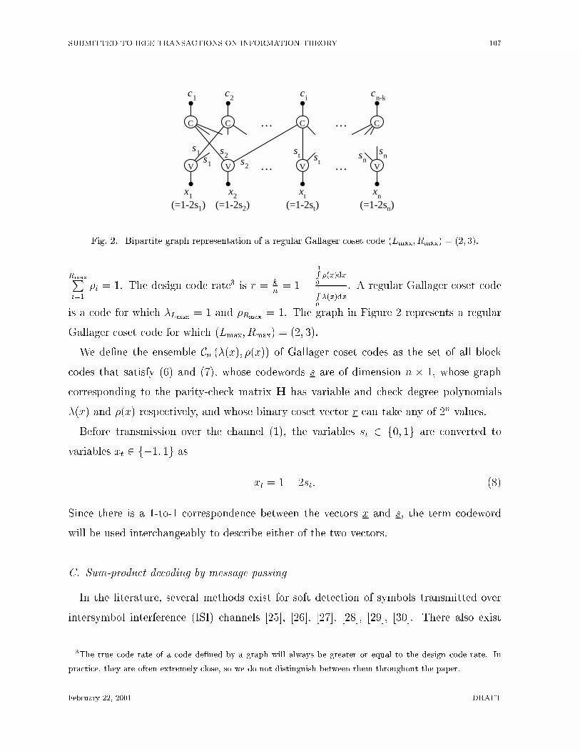
It is convenient to represent a Gallager coset code by a bipartite graph [12], [14], [23].
The graph has two types of nodes: n variable nodes (one variable node for each entry in
the vector s) and n�k check nodes (one check node for each entry in the vector c). There
is an edge connecting the i-th check node and the j-th variable node if the entry H(i; j)
in the i-th row and j-th column of H is non-zero. Thus, each check node represents a
parity check equation ci =L
j:H(i;j)6=0sj, where the symbol
Ldenotes binary addition. An
example of a graph of a Gallager coset code is depicted in Figure 2.
The degree of a node is the number of edges connected to it. Two degree polynomials
�(x) =LmaxPi=1
�ixi�1 and �(x) =
RmaxPi=1
�ixi�1 are de�ned [18], [20], where Lmax and Rmax
are the maximal variable and check node degrees respectively. If ne represents the total
number of edges in the graph, then the value �i represents the fraction of the ne edges
that are connected to variable nodes of degree i (�i is de�ned similarly). ClearlyLmaxPi=1
�i =
February 22, 2001 DRAFT
SUBMITTED TO IEEE TRANSACTIONS ON INFORMATION THEORY 107
c 1 c 2 c i c n-k
… …C CCC
… …V VVV
s 1 s 2 s t s ns 1 s 2s t
s n
xn(=1-2sn)
x1(=1-2s1)
x2(=1-2s2)
xt(=1-2st)
Fig. 2. Bipartite graph representation of a regular Gallager coset code (Lmax; Rmax) = (2; 3).
RmaxPi=1
�i = 1. The design code rate3 is r = kn= 1 �
1R
0
�(x)dx
1R
0
�(x)dx
. A regular Gallager coset code
is a code for which �Lmax = 1 and �Rmax = 1. The graph in Figure 2 represents a regular
Gallager coset code for which (Lmax; Rmax) = (2; 3).
We de�ne the ensemble Cn (�(x); �(x)) of Gallager coset codes as the set of all block
codes that satisfy (6) and (7), whose codewords s are of dimension n � 1, whose graph
corresponding to the parity-check matrix H has variable and check degree polynomials
�(x) and �(x) respectively, and whose binary coset vector r can take any of 2n values.
Before transmission over the channel (1), the variables st 2 f0; 1g are converted to
variables xt 2 f�1; 1g as
xt = 1� 2st: (8)
Since there is a 1-to-1 correspondence between the vectors x and s, the term codeword
will be used interchangeably to describe either of the two vectors.
C. Sum-product decoding by message passing
In the literature, several methods exist for soft detection of symbols transmitted over
intersymbol interference (ISI) channels [25], [26], [27], [28], [29], [30]. There also exist
3The true code rate of a code de�ned by a graph will always be greater or equal to the design code rate. In
practice, they are often extremely close, so we do not distinguish between them throughout the paper.
February 22, 2001 DRAFT
SUBMITTED TO IEEE TRANSACTIONS ON INFORMATION THEORY 108
c 1 c 2 c i c n-k
… …C CCC
… …V VVV
s 1 s 2 s t s ns 1 s 2s t
s n
…T …T TTq 0 q 1 q 2 q t-1 q t q n-1q n
x 1 x 2 x t x n
y 1 y 2 y t y n
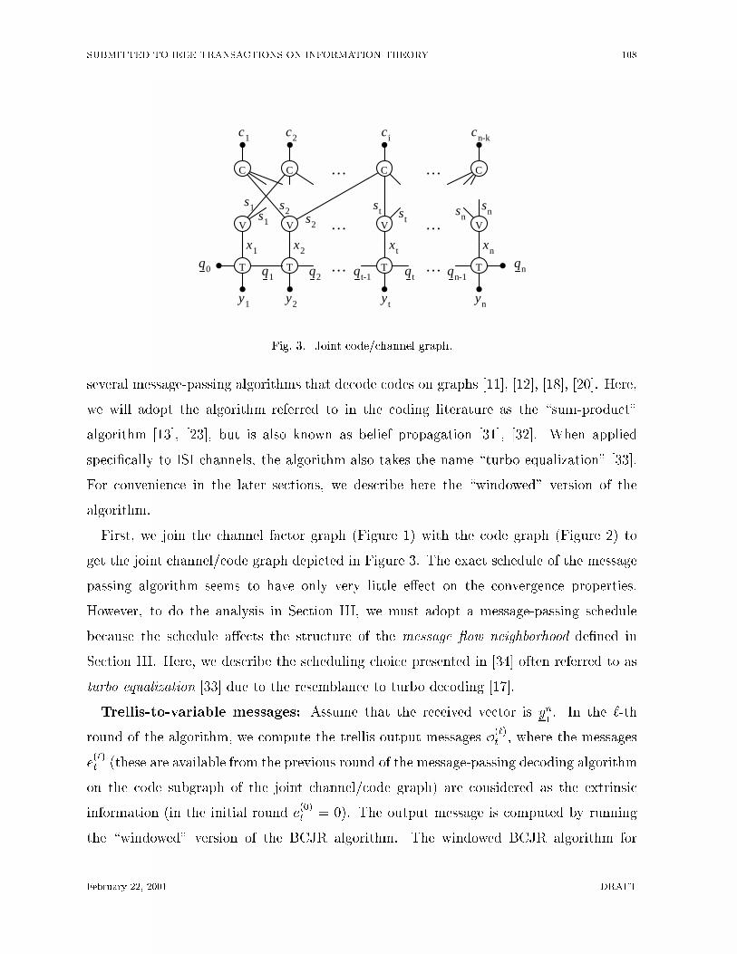
Fig. 3. Joint code/channel graph.
several message-passing algorithms that decode codes on graphs [11], [12], [18], [20]. Here,
we will adopt the algorithm referred to in the coding literature as the \sum-product"
algorithm [13], [23], but is also known as belief propagation [31], [32]. When applied
speci�cally to ISI channels, the algorithm also takes the name \turbo equalization" [33].
For convenience in the later sections, we describe here the \windowed" version of the
algorithm.
First, we join the channel factor graph (Figure 1) with the code graph (Figure 2) to
get the joint channel/code graph depicted in Figure 3. The exact schedule of the message
passing algorithm seems to have only very little e�ect on the convergence properties.
However, to do the analysis in Section III, we must adopt a message-passing schedule
because the schedule a�ects the structure of the message ow neighborhood de�ned in
Section III. Here, we describe the scheduling choice presented in [34] often referred to as
turbo equalization [33] due to the resemblance to turbo decoding [17].
Trellis-to-variable messages: Assume that the received vector is yn1. In the `-th
round of the algorithm, we compute the trellis output messages O(`)t , where the messages
e(`)t (these are available from the previous round of the message-passing decoding algorithm
on the code subgraph of the joint channel/code graph) are considered as the extrinsic
information (in the initial round e(0)t = 0). The output message is computed by running
the \windowed" version of the BCJR algorithm. The windowed BCJR algorithm for
February 22, 2001 DRAFT
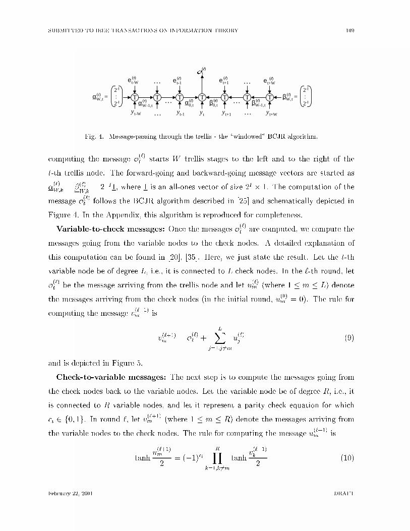
SUBMITTED TO IEEE TRANSACTIONS ON INFORMATION THEORY 109
T TT TT TTαW, t =(O) βW, t =
(O)
βW-1, t(O)β0, t
(O)
2-I
:2-I
2-I
:2-Iα0, t
(O)αW-1, t(O) ……
… …y tyt-1 y t+1y t-W y t+W
2 t(O)
e t-W(O) e t-1
(O) e t+1(O) e t+W
(O)……
Fig. 4. Message-passing through the trellis - the \windowed" BCJR algorithm.
computing the message O(`)t starts W trellis stages to the left and to the right of the
t-th trellis node. The forward-going and backward-going message vectors are started as
�(`)W;k = �(`)
W;k= 2�I1, where 1 is an all-ones vector of size 2I � 1. The computation of the
message O(`)t follows the BCJR algorithm described in [25] and schematically depicted in
Figure 4. In the Appendix, this algorithm is reproduced for completeness.
Variable-to-check messages: Once the messages O(`)t are computed, we compute the
messages going from the variable nodes to the check nodes. A detailed explanation of
this computation can be found in [20], [35]. Here, we just state the result. Let the t-th
variable node be of degree L, i.e., it is connected to L check nodes. In the `-th round, let
O(`)t be the message arriving from the trellis node and let u(`)m (where 1 � m � L) denote
the messages arriving from the check nodes (in the initial round, u(0)m = 0). The rule for
computing the message v(`+1)m is
v(`+1)m = O(`)t +LX
j=1;j 6=mu(`)j (9)
and is depicted in Figure 5.
Check-to-variable messages: The next step is to compute the messages going from
the check nodes back to the variable nodes. Let the variable node be of degree R, i.e., it
is connected to R variable nodes, and let it represent a parity check equation for which
ci 2 f0; 1g. In round `, let v(`+1)m (where 1 � m � R) denote the messages arriving from
the variable nodes to the check nodes. The rule for computing the message u(`+1)m is
tanhu(`+1)m
2= (�1)ci
RYk=1;k 6=m
tanhv(`+1)k
2(10)
February 22, 2001 DRAFT
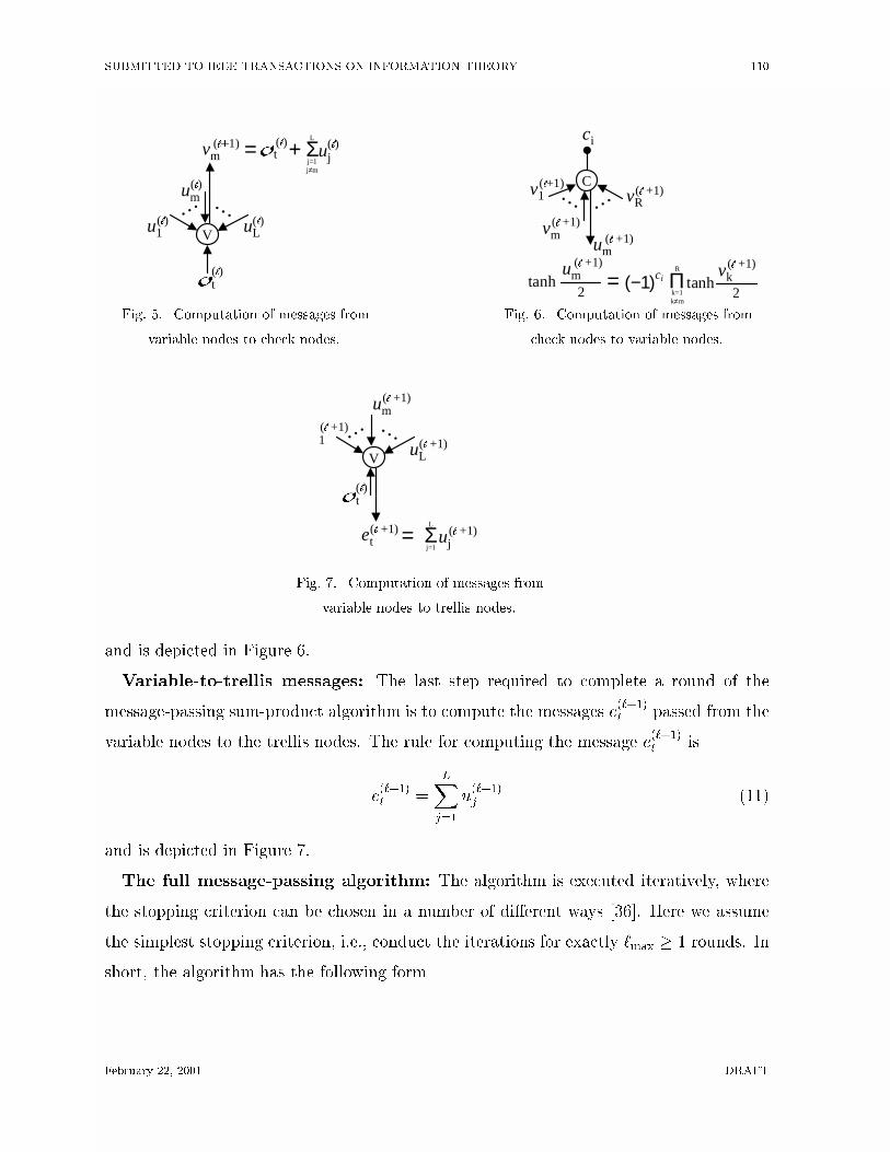
SUBMITTED TO IEEE TRANSACTIONS ON INFORMATION THEORY 110
(O)
V
2 t
u1(O)
um(O)
uL(O)
vm(O�1)
… …
= + Σuj (O)
L
j=1j≠m
(O)2 t
Fig. 5. Computation of messages from
variable nodes to check nodes.
Cv1(O+1)
vm(O +1)
vR(O +1)
um(O +1)
……
= (−1)ci Π tanhR
k=1k≠m
2tanh
vk(O +1)
2
um(O +1)
ci
Fig. 6. Computation of messages from
check nodes to variable nodes.
(O)
V
2 t
1(O +1)
um(O +1)
uL(O +1)
et(O +1)
… …
= Σ uj
(O +1)
L
j=1
Fig. 7. Computation of messages from
variable nodes to trellis nodes.
and is depicted in Figure 6.
Variable-to-trellis messages: The last step required to complete a round of the
message-passing sum-product algorithm is to compute the messages e(`+1)t passed from the
variable nodes to the trellis nodes. The rule for computing the message e(`+1)t is
e(`+1)t =
LXj=1
u(`+1)j (11)
and is depicted in Figure 7.
The full message-passing algorithm: The algorithm is executed iteratively, where
the stopping criterion can be chosen in a number of di�erent ways [36]. Here we assume
the simplest stopping criterion, i.e., conduct the iterations for exactly `max � 1 rounds. In
short, the algorithm has the following form
February 22, 2001 DRAFT
SUBMITTED TO IEEE TRANSACTIONS ON INFORMATION THEORY 111
� Initialization
1. receive channel outputs y1; y2; : : : ; yt; : : : ; yn.
2. for 1 � t � n, set e(0)t = 0.
3. set all check-to-variable messages u(0)m = 0.
4. set ` = 0.
� Repeat while ` < `max
1. for 1 � t � n compute all trellis-to-variable messages O(`)t [Figure 4 and the Appendix].
2. compute all variable-to-check messages v(`+1)m [Figure 5 and equation (9)].
3. compute all check-to-variable messages u(`+1)m [Figure 6 and equation (10)].
4. for 1 � t � n compute all variable-to-trellis messages e(`+1)t [Figure 7 and equa-
tion (11)].
5. increment ` by 1.
� Decode
1. for 1 � t � n decide xt = sign�O(`max�1)t + e(`max)
t
�.
III. Concentration and the \Zero-Error" Threshold
In this section, we will prove that for information sequences generated uniformly at
random, for almost all graphs and almost all cosets, the decoder behaves very closely to
the expected behavior. The expected behavior is de�ned as the behavior of the decoder
when the channel input is a sequence of equally likely i.i.d. random variables. We will
then conclude that there exists at least one graph and one coset for which the decoding
probability of error can be made arbitrarily small on an information sequence generated
uniformly at random if the noise variance does not exceed a threshold. The proofs follow
closely the ideas presented in [19], [20] for memoryless channels and rely heavily on results
presented there. The main di�erence is that the channel under consideration here has an
input-dependent memory. Therefore, we �rst must prove a concentration statement for
every possible input sequence, and then show that the average decoder performance is
closely concentrated around the decoder performance when the input sequence is i.i.d.
The section is organized as follows. In subsection III-A, the basic notation is introduced.
Subsection III-B gives the concentration result, while subsection III-C de�nes the \zero-
February 22, 2001 DRAFT
SUBMITTED TO IEEE TRANSACTIONS ON INFORMATION THEORY 112
e
1 0 10
Ce
Ve
T T T
VV
C C CC
V
C
V VVV V…
ve(O�1)
Equivalentrepresentations
=
Ce
Ve
VV …
0 1 0 1
2W+I+1symbols
L-1
R-1
LL
R-1R-1
a) b)
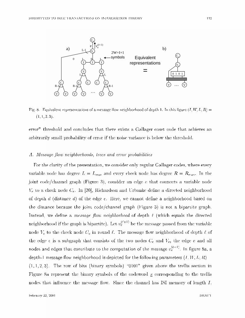
Fig. 8. Equivalent representations of a message ow neighborhood of depth 1. In this �gure (I;W;L;R) =
(1; 1; 2; 3).
error" threshold and concludes that there exists a Gallager coset code that achieves an
arbitrarily small probability of error if the noise variance is below the threshold.
A. Message ow neighborhoods, trees and error probabilities
For the clarity of the presentation, we consider only regular Gallager codes, where every
variable node has degree L = Lmax and every check node has degree R = Rmax. In the
joint code/channel graph (Figure 3), consider an edge e that connects a variable node
Ve to a check node Ce. In [20], Richardson and Urbanke de�ne a directed neighborhood
of depth d (distance d) of the edge e. Here, we cannot de�ne a neighborhood based on
the distance because the joint code/channel graph (Figure 3) is not a bipartite graph.
Instead, we de�ne a message ow neighborhood of depth ` (which equals the directed
neighborhood if the graph is bipartite). Let v(`+1)e be the message passed from the variable
node Ve to the check node Ce in round `. The message ow neighborhood of depth ` of
the edge e is a subgraph that consists of the two nodes Ce and Ve, the edge e and all
nodes and edges that contribute to the computation of the message v(`+1)e . In �gure 8a, a
depth-1 message ow neighborhood is depicted for the following parameters (I;W; L;R) =
(1; 1; 2; 3). The row of bits (binary symbols) \0101" given above the trellis section in
Figure 8a represent the binary symbols of the codeword s corresponding to the trellis
nodes that in uence the message ow. Since the channel has ISI memory of length I,
February 22, 2001 DRAFT
SUBMITTED TO IEEE TRANSACTIONS ON INFORMATION THEORY 113
Ve
VV …
0 1 0 1
Ce
V
VV …
0 0 0 0
V
VV …
1 1 1 0
V
VV …
1 0 0 1
…
V
…
1 1 1 1
VV…
Stage 1
Stage O-1
Stage O
…
…
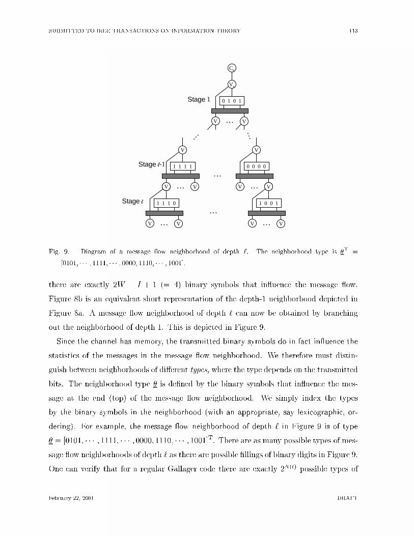
Fig. 9. Diagram of a message ow neighborhood of depth `. The neighborhood type is �T =
[0101; � � � ; 1111; � � � ; 0000; 1110; � � � ; 1001].
there are exactly 2W + I + 1 (= 4) binary symbols that in uence the message ow.
Figure 8b is an equivalent short representation of the depth-1 neighborhood depicted in
Figure 8a. A message ow neighborhood of depth ` can now be obtained by branching
out the neighborhood of depth 1. This is depicted in Figure 9.
Since the channel has memory, the transmitted binary symbols do in fact in uence the
statistics of the messages in the message ow neighborhood. We therefore must distin-
guish between neighborhoods of di�erent types, where the type depends on the transmitted
bits. The neighborhood type � is de�ned by the binary symbols that in uence the mes-
sage at the end (top) of the message ow neighborhood. We simply index the types
by the binary symbols in the neighborhood (with an appropriate, say lexicographic, or-
dering). For example, the message ow neighborhood of depth ` in Figure 9 is of type
� = [0101; � � � ; 1111; � � � ; 0000; 1110; � � � ; 1001]T. There are as many possible types of mes-
sage ow neighborhoods of depth ` as there are possible �llings of binary digits in Figure 9.
One can verify that for a regular Gallager code there are exactly 2N(`) possible types of
February 22, 2001 DRAFT
SUBMITTED TO IEEE TRANSACTIONS ON INFORMATION THEORY 114
message ow neighborhoods of depth `, where
N(`) = (2W + I + 1) �(R� 1)`(2WL+ L� 1)` � 1
(R� 1)(2WL+ L� 1)� 1: (12)
We index these neighborhoods as �i 2 f0; 1gN(`), where 1 � i � 2N(`).
A tree-like neighborhood, or simply a tree of depth ` is a message ow neighborhood of
depth ` in which all nodes appear only once. In other words, a tree of depth ` is a message
ow neighborhood that contains no loops. Just like message ow neighborhoods, the trees
of depth ` can be of any of the 2N(`) types �i 2 f0; 1gN(`), where 1 � i � 2N(`).
De�ne s� as the binary symbol corresponding to the message node Ve at the top of the
message ow neighborhood of type �. In Figure 8a, the symbol s� can be read as the
symbol directly below the node Ve, i.e., s� = 0. The corresponding value of the symbol
is x� = 1 � 2s� = 1. De�ne �(`)� as the probability that the tree of type � and depth `
delivers an incorrect message, i.e.,
�� = Pr�v(`+1)e � x� < 0 j tree type �
�(13)
The probability in (13) is taken over all possible outcomes of the channel outputs when �
is the tree type, i.e., when the binary symbols that de�ne � are transmitted.
We de�ne the probability Pr (�js) as the probability that a message ow neighborhood
(of a random edge) is of type � when the transmitted n-long sequence is s and the code
graph is chosen uniformly at random from all possible graphs with degree polynomials
�(x) and �(x), i.e.,
Pr (�js) = Pr (neighborhood type = � j transmitted sequence = s) : (14)
Note that the probability de�ned in (14) does not depend on the coset r; also note that
there always exists a vector r such that for any chosen parity check matrix H the vector
s is a codeword of the coset code speci�ed by H and r.
Next, de�ne the error concentration probability when s is the transmitted sequence as
p(`)(s) =2N(`)Xi=1
�(`)�iPr (�ijs) : (15)
February 22, 2001 DRAFT
SUBMITTED TO IEEE TRANSACTIONS ON INFORMATION THEORY 115
De�ne the i.i.d. error concentration probability p(`)i:i:d: as the error concentration probability
when all possible 2N(`) neighborhood types �i, 1 � i � 2N(`), are equally probable
p(`)i:i:d: =
2N(`)Xi=1
�(`)�i2�N(`): (16)
In the next subsection, we prove that for most graphs, if s is the transmitted codeword,
then the probability of a variable-to-check message being erroneous after ` rounds of the
message-passing decoding algorithm is highly concentrated around the value p(`)(s). Also,
we prove that if the transmitted sequence is i.i.d., then the probability of a variable-to-
check message being erroneous after ` rounds of the message-passing decoding algorithm
is highly concentrated around the value p(`)i:i:d:. To do that we need the following result
from [20]. De�ne Pt as the probability that a neighborhood of depth ` is not a tree when a
code graph is chosen uniformly at random from all possible graphs with degree polynomials
�(x) and �(x). In [20] it is shown that
Pt = Pr (neighborhood not a tree) �
n; (17)
where is a constant independent of n.4
B. Concentration theorems
Theorem 1: Let s be the transmitted codeword. Let Z(`) (s) be the random variable that
denotes the number of erroneous messages after ` rounds of the message-passing decoding
algorithm when the code graph is chosen uniformly at random from the ensemble of graphs
with degree polynomials �(x) and �(x). Let ne be the number of variable-to-check edges
in the graph. For an arbitrarily small constant " > 0, there exists a positive number �,
such that if n > 2 ", then
Pr
�����Z(s)ne� p(`)s
���� � "
�� e��"
2n: (18)
4Actually, in [20] this fact is shown for a bipartite graph, but the extension to joint code/channel graphs of
Figure 3 is straight-forward.
February 22, 2001 DRAFT
SUBMITTED TO IEEE TRANSACTIONS ON INFORMATION THEORY 116
Proof: The proof follows closely the proof of the concentration theorem for
memoryless channels presented in [20]. First note that
Pr
�����Z(`)(s)
ne� p(`)(s)
���� � "
��
Pr
�����Z(`)(s)
ne�
E�Z(`)(s)
�ne
����� � "
2
!+ Pr
�����E�Z(`)(s)
�ne
� p(`)(s)
����� � "
2
!: (19)
The random variable Z(`)(s) depends on the deterministic sequence s and its probability
space is the union of the ensemble of graphs with degree polynomials �(x), �(x) and the
ensemble of channel noise realizations (which uniquely de�ne the channel outputs since s
is known). Following [20], we form a Doob edge-and-noise-revealing martingale and apply
Azuma's inequality [37] to get
Pr
�����Z(`)(s)
ne�
E�Z(`)(s)
�ne
����� � "
2
!� 2e��"
2n; (20)
where � depends only on �(x), �(x) and `.
Next, we show that the second term on the right-hand side of (19) equals to 0, by using
the result in (17). Again, this is adopted from [20], but adapted to a channel with ISI
memory. We have
E�Z(`)(s)
�� ne(1� Pt)
2N(`)Xi=1
�(`)�iPr (�ijs) + ne
n
� ne
2N(`)Xi=1
�(`)�iPr (�ijs) + ne
n
� nep(`)(s) + ne
n(21)
and
E�Z(`)(s)
�� ne(1� Pt)
2N(`)Xi=1
�(`)�iPr (�ijs)
� ne
2N(`)Xi=1
�(`)�iPr��ijs�� nePt
2N(`)Xi=1
Pr (�ijs)
� nep(`)(s)� ne
n: (22)
February 22, 2001 DRAFT
SUBMITTED TO IEEE TRANSACTIONS ON INFORMATION THEORY 117
Combining (21) and (22), if n > 2 ", we get
Pr
�����E�Z(`)(s)
�ne
� p(`)(s)
����� � "
2
!= 0: (23)
Theorem 2: Let S be a random sequence of i.i.d. equally likely binary random variables
(symbols) S1; S2; : : : ; Sn. Let Z(`) (S) be the random variable that denotes the number
of erroneous messages after ` rounds of the message-passing decoding algorithm when
the code graph is chosen uniformly at random from the ensemble of graphs with degree
polynomials �(x) and �(x), and when the transmitted sequence is S. Let ne be the number
of variable-to-check edges in the graph. For an arbitrarily small constant " > 0, there exists
a positive number � 0, such that if n > 2 ", then
Pr
�����Z(S)ne� p
(`)i:i:d:
���� � "
�� 4e��
0"2n: (24)
Proof: Using Theorem 1, we have the following
Pr
�����Z(`)(S)
ne� p
(`)i:i:d:
���� � "
�=
2nXj=1
2�nPr
�����Z(`)(sj)
ne� p
(`)i:i:d:
����� � "
!
�2nXj=1
2�nPr
�����Z(`)(sj)
ne� p(`)(sj)
����� � "
2
!
+2nXj=1
2�nPr����p(`)(sj)� p
(`)i:i:d:
��� � "
2
�
�2nXj=1
2�n � 2e��"2n=4 + Pr
����p(`)(S)� p(`)i:i:d:
��� � "
2
�
= 2e��"2n=4 + Pr
����p(`)(S)� p(`)i:i:d:
��� � "
2
�: (25)
Next, recognize that if S is an i.i.d. random sequence, all neighborhood types are equally
probable, i.e., Pr (�ijS) = 2�N(`). Using this, we prove that E�p(`)(S)
�= p
(`)i:i:d:,
E�p(`)(S)
�=
2nXj=1
2�np(`)(sj) =2nXj=1
2�n2N(`)Xi=1
�(`)�iPr��ijsj
�
=2N(`)Xi=1
�(`)�i
2nXj=1
2�nPr��ijsj
�=
2N(`)Xi=1
�(`)�iPr (�ijS) =
2N(`)Xi=1
�(`)�i2�N(`) = p
(`)i:i:d::
February 22, 2001 DRAFT
SUBMITTED TO IEEE TRANSACTIONS ON INFORMATION THEORY 118
Now form a Doob symbol-revealing martingale sequence M0;M1; : : : ;Mn
Mt = E�p(`)(S) j S1; S2; : : : ; St
�M0 = E
�p(`)(S)
�= p(`)i:i:d:
Mn = E�p(`)(S) j S
�= p(`)(S):
If we can show that
jMt+1 �Mtj �Æ
n; (26)
where Æ is a constant dependent on �(x), �(x) and ` (but not dependent on n) then if we
apply Azuma's inequality [37], we will have
Pr����p(`)(S)� p
(`)i:i:d:
��� � "
2
�� 2e�(8Æ
2)�1
"2n: (27)
Then, by combining (27) and (25), for � 0 = min��4; 18Æ2
�, we will get (24). So, all that
needs to be shown is (26).
Consider two random variables p(`)(S) and p(`)( ~S). The random vectors S and ~S have
the following properties: 1) the �rst t symbols of S and ~S are deterministic and equal
St
1 = ~St
1 = st1; 2) The (t+1)-th symbol of S is the random variable St, while the (t+1)-th
symbol of ~S is �xed (non-random) ~St+1 = st+1; 3) the remaining symbols Sn
t+2 and ~Sn
t+2
are i.i.d. binary random vectors. Fixing the (t + 1)-th symbol ~St+1 = st+1 can a�ect at
most a constant number (call this number �) of message- ow neighborhoods of depth `.
The constant � depends on �(x), �(x) and `, but it does not depend on n. Therefore, for
any given neighborhood type �i, we have���Pr��ijS�� Pr��ij ~S
���� � �
ne: (28)
Using the notation �0(1) = @�(x)@x
���x=1
, we can verify that ne = [�0(1) + 1]n. De�ning
Æ = 2N(`)���0(1)+1
, and using (28), we get
���p(`)(S)� p(`)( ~S)��� �
2N(`)Xi=1
���Pr��ijS�� Pr��ij ~S
����� 2N(`) �
ne=
Æ
n: (29)
February 22, 2001 DRAFT
SUBMITTED TO IEEE TRANSACTIONS ON INFORMATION THEORY 119
Inequality (26) follows from (29).
Corollary 2.1: Letm be an information block chosen uniformly at random from 2k = 2rn
binary sequences of length k. Let C (H; r) be a code chosen uniformly at random from the
ensemble Cn (�(x); �(x)) of Gallager coset codes. Let Z(`) be a random variable representing
the number of erroneous variable-to-check messages in round ` of the message-passing
decoding algorithm on the joint channel/code of the code C (H; r). Then
Pr
�����Z(`)
ne� p
(`)i:i:d:
���� � "
�� 4e��
0"2n: (30)
Proof: If m, H and r are all chosen uniformly at random, then the resulting
codeword in (6) is an i.i.d. random sequence of equally likely binary random symbols, and
Theorem 2 applies directly.
C. \Zero-error" threshold
The term \zero-error" threshold is a slight abuse because the decoding error can never
be made equal to zero, but the concentration probability can be equal to zero in the limit
as `!1, and hence the probability of decoding error can be made arbitrarily small. As
in [20], the \zero-error" noise standard deviation threshold �� is de�ned as
�� = sup �; (31)
where the supremum in (31) is taken over all noise standard deviations � for which
lim`!1
p(`)i:i:d: = 0: (32)
Corollary 2.2: Letm be an information block chosen uniformly at random from 2k = 2rn
binary sequences of length k. There exists a code C (H; r) in the ensemble Cn (�(x); �(x))
of Gallager coset codes, such that for any � < �� the probability of error can be made
arbitrarily low, i.e., if Z(`) is the number of erroneous variable-to-check messages in round `
of the message-passing decoding algorithm on the joint channel/code of the code C (H; r),
then
Pr
�Z(`)
ne� 2" j C (H; r)
�� 4e��
0"2n: (33)
February 22, 2001 DRAFT
SUBMITTED TO IEEE TRANSACTIONS ON INFORMATION THEORY 120
Proof: De�ne an indicator random variable
I�Z(`)
�=
8<: 1 if
���Z(`)
ne� p(`)i:i:d:
��� � "
0 otherwise(34)
From Corollary 2.1, for H, r and m chosen uniformly at random we have E�I�Z(`)
���
4e��0"2n. Since the expected value is lower than 4e��
0"2n, we conclude that there must exist
at least one graph H and one coset-de�ning vector r such that for m chosen uniformly
at random we have E�I�Z(`)
�j C(H; r)
�� 4e��
0"2n, i.e., there exists a graph H and a
coset-de�ning vector r such that for m chosen uniformly at random
Pr
�����Z(`)
ne� p
(`)i:i:d:
���� � " j C (H; r)
�� 4e��
0"2n: (35)
The assumption � < �� guarantees lim`!1
p(`)i:i:d: = 0. Since lim
`!1p(`)i:i:d: = 0, it follows that for
every " > 0, there exists an integer `(") such that for every ` � `(") we have p(`)i:i:d: � ".
Then for ` � `("), we have
Pr
�Z(`)
ne� 2"
�� Pr
�����Z(`)
ne� p
(`)i:i:d:
���� � "
�: (36)
The desired result (33) follows by combining (35) and (36).
IV. Density Evolution and Threshold Computation
A. Density evolution
De�ne f(`+1)V j� (�j�) as the probability density function (pdf) of the message v
(`+1)e obtained
at the top of a depth-` tree of type �, see Figure 8. With this notation, we may express
February 22, 2001 DRAFT
SUBMITTED TO IEEE TRANSACTIONS ON INFORMATION THEORY 121
the i.i.d. error concentration probability as
p(`)i:i:d: =
2N(`)Xi=1
2�N(`)�(`)�i
=2N(`)Xi=1
2�N(`)
0Z�1
f (`+1)V j�i (�j�i) � x�i � d�
=
0Z�1
242N(`)X
i=1
2�N(`)f(`+1)V j�i (�j�i) � x�i
35 d�
=
0Z�1
f(`+1)V (�)d�: (37)
Here, f(`+1)V (�) is the average probability density function (averaged over all tree types) of
the correct message from a variable node to a check node in round ` of the message-passing
algorithm on a tree. We can obtain the pdf f(`+1)V (�) in several di�erent ways. Here we
perform the averaging in every round and enter a new round with an average pdf from the
previous round, i.e., we evolve f(`)V (�) into f
(`+1)V (�). This method is used in [9] for discrete
messages and in [20] for continuous messages, where it was termed density evolution.
Denote by f(`)O (�) the average density (pdf) of a message O(`)t in the `-th round of the
message-passing algorithm (averaged over all tree types), see Figure 5. Let f(`)U (�) denote
the average pdf of a message u(`)m in the `-th round of the message-passing algorithm on a
tree. Then the average density (pdf) f(`+1)V (�) is given by
f(`+1)V (�) = f
(`)O (�)
"LmaxXi=1
�i
i�1Ok=1
f(`)U (�)
!#; (38)
where stands for the convolution operation, andi�1Nk=1
denotes the convolution of i � 1
pdf's. For short notation, we use the following
��f(`)U (�)
�=
LmaxXi=1
�i
i�1Ok=1
f(`)U (�)
!: (39)
We also drop the function argument � since it is common for all convolved pdf's. Then (38)
may be conveniently expressed as
f(`+1)V = f
(`)O �
�f(`)U
�: (40)
February 22, 2001 DRAFT
SUBMITTED TO IEEE TRANSACTIONS ON INFORMATION THEORY 122
Equation (40) denotes the evolution of the average density (pdf) through a variable node,
Figure 5.
To express the density evolution through a check node (Figure 6), we require a variable
change, resulting in a cumbersome change of measure. A convolution can then be de�ned
in the new domain and an expression can be found for the density evolution through check
nodes [20]. Here we do not pursue this rather complicated procedure because a numerical
method for density evolution through check nodes can easily be obtained through a table-
lookup, for details see [22]. Here we simply denote this density evolution as
f(`+1)U =
RmaxXi=1
�iEi�1c
�f(`+1)V
�; (41)
where E i�1c
�f(`+1)V
�is symbolic notation for the average message density obtained by
evolving the density f(`+1)V (�) through a check node of degree i. We further express equa-
tion (41) by the following notation
f(`+1)U = �
hEc�f(`+1)V
�i: (42)
Similar to equation (40), the average density (pdf) of messages e(`+1)t (Figure 7) is obtained
using the convolution operator
f (`+1)E = f (`+1)U ��f (`+1)U
�: (43)
The step that is needed to close the loop of a single density evolution round is the evolution
of the average density f(`+1)E into the average density f
(`+1)O , i.e., the evolution of message
densities through the trellis portion of the joint code/channel graph. We denote this step
as
f(`+1)O = Et
�f(`+1)E ; fN
�; (44)
where Et is symbolic notation for trellis evolution and fN denotes the pdf of the channel
noise (in this case a zero-mean Gaussian with variance �2). Even though no closed form
solution for (44) is known, it can be calculated numerically.
February 22, 2001 DRAFT
SUBMITTED TO IEEE TRANSACTIONS ON INFORMATION THEORY 123
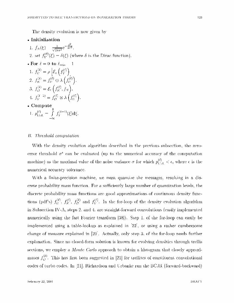
The density evolution is now given by
� Initialization
1. fN(�) =1p2��2
e��2
2�2 .
2. set f(0)V (�) = Æ(�) (where Æ is the Dirac function).
� For ` = 0 to `max � 1
1. f(`)U = �
hEc
�f(`)V
�i2. f
(`)E = f
(`)U �
�f(`)U
�.
3. f(`)O = Et
�f(`)E ; fN
�.
4. f(`+1)V = f
(`)O �
�f(`)U
�.
� Compute
1. p(`)i:i:d: =
0R�1
f(`+1)V (�)d�.
B. Threshold computation
With the density evolution algorithm described in the previous subsection, the zero-
error threshold �� can be evaluated (up to the numerical accuracy of the computation
machine) as the maximal value of the noise variance � for which p(`)i:i:d: < �, where � is the
numerical accuracy tolerance.
With a �nite-precision machine, we must quantize the messages, resulting in a dis-
crete probability mass function. For a suÆciently large number of quantization levels, the
discrete probability mass functions are good approximations of continuous density func-
tions (pdf's) f(`)U , f
(`)E , f
(`)O and f
(`)V . In the for-loop of the density evolution algorithm
in Subsection IV-A, steps 2. and 4. are straight-forward convolutions (easily implemented
numerically using the fast Fourier transform [38]). Step 1. of the for-loop can easily be
implemented using a table-lookup as explained in [22], or using a rather cumbersome
change of measure explained in [20]. Actually, only step 3. of the for-loop needs further
explanation. Since no closed-form solution is known for evolving densities through trellis
sections, we employ a Monte Carlo approach to obtain a histogram that closely approxi-
mates f(`)O . This has �rst been suggested in [21] for trellises of constituent convolutional
codes of turbo codes. In [21], Richardson and Urbanke run the BCJR (forward-backward)
February 22, 2001 DRAFT
SUBMITTED TO IEEE TRANSACTIONS ON INFORMATION THEORY 124
algorithm on a long trellis section when the input is the all-zero sequence. Here, since the
channel has memory, the transmitted sequence must be a randomly chosen i.i.d. binary
sequence of equally likely symbols. The length n of the sequence must be very long so
that we can ignore the trellis boundary e�ects. For each binary symbol xt we compute the
trellis-output information O(`)t according to the BCJR algorithm. We then equate f(`)O to
the histogram of the values O(`)t � xt, where K � t � n�K, and K is chosen large enough
to avoid the trellis boundary e�ects. In [21] this technique is accelerated by forcing the
consistency condition on the histogram. In ISI channels, however, consistency generally
does not hold, so we must use a larger trellis section in the Monte Carlo simulation.
V. Achievable rates of Gallager codes
A. Achievable rates of binary linear codes over ISI channels
In section II, we pointed out that Ci:i:d: is the limitation of the average mutual informa-
tion betweenXn1 and Y
n1 whenX
n1 is an i.i.d. sequence with Pr (Xt = �1) = Pr (Xt = +1) =
12. Since the input process, the channel and hence the output process and the joint input-
output process are all stationary and ergodic, one can adopt the standard random coding
technique [1] to prove a coding theorem to assure that all rates r < Ci:i:d: are achievable
(for the de�nition of achievable, see [2], p. 194). We use the expression \standard random
coding technique" to describe a method to generate the code book, where codewords are
chosen independently at random and the coded symbols are governed by the optimal input
distribution. For a generic �nite-state channel, see [1] Section 5.9 or [39] for a detailed
description of the problem and the the proof of the coding theorem. For the channel in (1)
with binary inputs, we present a somewhat stronger result involving linear codes.5
5Here we use a di�erent (what also appear to be a simpler) proof methodology. However, the proof only applies
to �nite-state channels for which we can guarantee that we can achieve any state with a �nite number of channel
inputs (e.g., ISI channels with �nite ISI memory), not for a general �nite-state channel.
February 22, 2001 DRAFT
SUBMITTED TO IEEE TRANSACTIONS ON INFORMATION THEORY 125
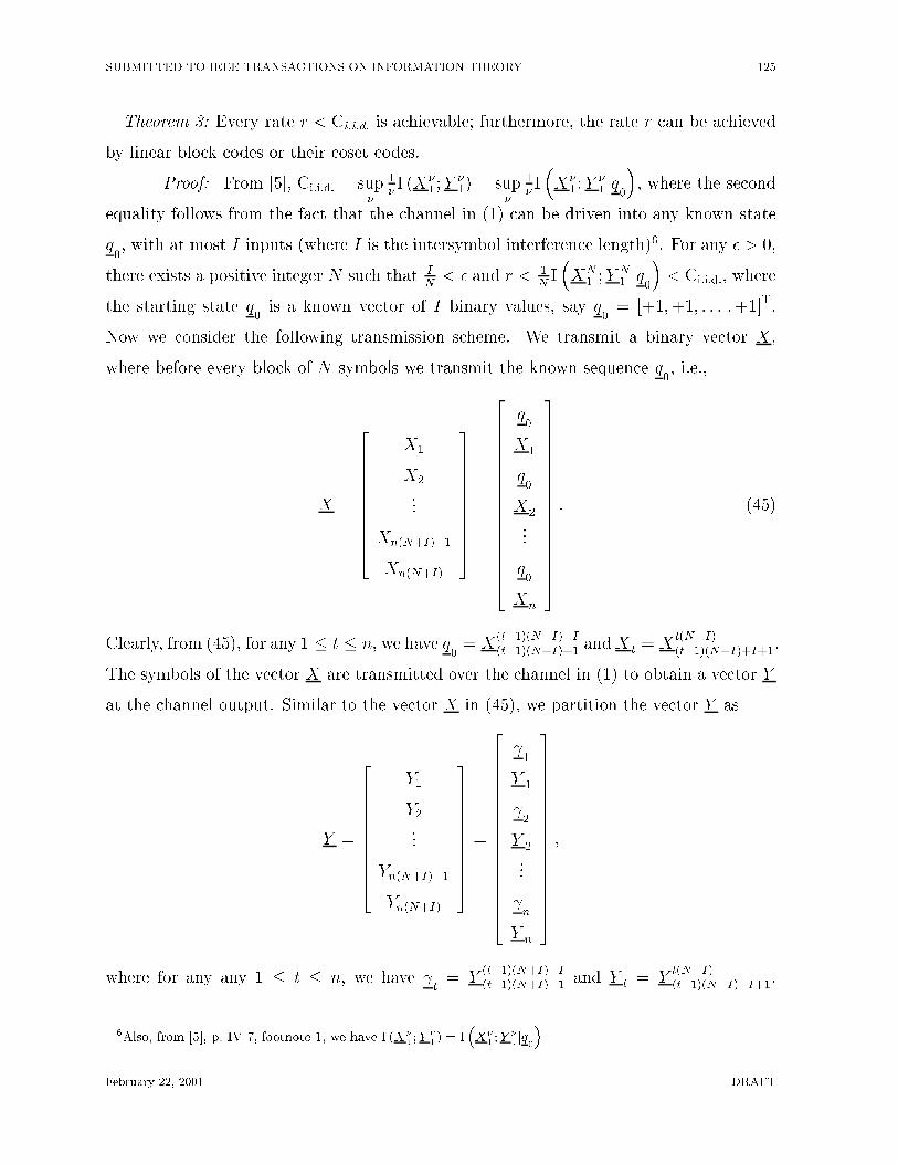
Theorem 3: Every rate r < Ci:i:d: is achievable; furthermore, the rate r can be achieved
by linear block codes or their coset codes.
Proof: From [5], Ci:i:d: = sup�
1�I (X�
1;Y�1) = sup
�
1�I�X�
1;Y�1jq0
�, where the second
equality follows from the fact that the channel in (1) can be driven into any known state
q0, with at most I inputs (where I is the intersymbol interference length)6. For any � > 0,
there exists a positive integer N such that IN< � and r < 1
NI�XN
1 ;YN1 jq0
�< Ci:i:d:, where
the starting state q0is a known vector of I binary values, say q
0= [+1;+1; : : : ;+1]T.
Now we consider the following transmission scheme. We transmit a binary vector X,
where before every block of N symbols we transmit the known sequence q0, i.e.,
X =
2666666664
X1
X2
...
Xn(N+I)�1
Xn(N+I)
3777777775=
2666666666666664
q0
X1
q0
X2
...
q0
Xn
3777777777777775
: (45)
Clearly, from (45), for any 1 � t � n, we have q0= X
(t�1)(N+I)+I(t�1)(N+I)+1 andX t = X
t(N+I)(t�1)(N+I)+I+1.
The symbols of the vector X are transmitted over the channel in (1) to obtain a vector Y
at the channel output. Similar to the vector X in (45), we partition the vector Y as
Y =
2666666664
Y1
Y2...
Yn(N+I)�1
Yn(N+I)
3777777775=
2666666666666664
1
Y 1
2
Y 2
...
n
Y n
3777777777777775
;
where for any any 1 � t � n, we have t= Y
(t�1)(N+I)+I(t�1)(N+I)+1 and Y t = Y
t(N+I)(t�1)(N+I)+I+1.
6Also, from [5], p. IV-7, footnote 1, we have I (X�1 ; Y
�1) = I
�X�
1 ;Y�1 jq
0
�
February 22, 2001 DRAFT
SUBMITTED TO IEEE TRANSACTIONS ON INFORMATION THEORY 126
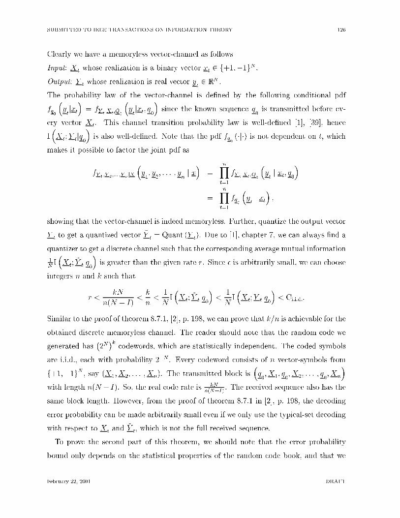
Clearly we have a memoryless vector-channel as follows
Input: X t whose realization is a binary vector xt 2 f+1;�1gN .
Output: Y t whose realization is real vector yt2 RN .
The probability law of the vector-channel is de�ned by the following conditional pdf
fq0
�ytjxt
�= fY tjXt;Q0
�ytjxt; q0
�since the known sequence q
0is transmitted before ev-
ery vector Xt. This channel transition probability law is well-de�ned [1], [39], hence
I�X t;Y tjq0
�is also well-de�ned. Note that the pdf fq
0(�j�) is not dependent on t, which
makes it possible to factor the joint pdf as
fY 1;Y 2;::: ;Y njX�y1; y
2; : : : ; y
nj x�
=nYt=1
fY tjXt;Q0
�ytj xt; q0
�
=nYt=1
fq0
�ytj xt
�;
showing that the vector-channel is indeed memoryless. Further, quantize the output vector
Y t to get a quantized vector ~Y t = Quant (Y t). Due to [1], chapter 7, we can always �nd a
quantizer to get a discrete channel such that the corresponding average mutual information
1NI�X t; ~Y tjq0
�is greater than the given rate r. Since � is arbitrarily small, we can choose
integers n and k such that
r <kN
n(N + I)<
k
n<
1
NI�X t; ~Y tjq0
�<
1
NI�X t;Y tjq0
�< Ci:i:d::
Similar to the proof of theorem 8.7.1, [2], p. 198, we can prove that k=n is achievable for the
obtained discrete memoryless channel. The reader should note that the random code we
generated has�2N�k
codewords, which are statistically independent. The coded symbols
are i.i.d., each with probability 2�N . Every codeword consists of n vector-symbols from
f+1;�1gN , say (X1; X2; : : : ; Xn). The transmitted block is�q0; X1; q0; X2; : : : ; q0; Xn
�with length n(N + I). So, the real code rate is kN
n(N+I). The received sequence also has the
same block length. However, from the proof of theorem 8.7.1 in [2], p. 198, the decoding
error probability can be made arbitrarily small even if we only use the typical-set decoding
with respect to X t and ~Y t, which is not the full received sequence.
To prove the second part of this theorem, we should note that the error probability
bound only depends on the statistical properties of the random code book, and that we
February 22, 2001 DRAFT
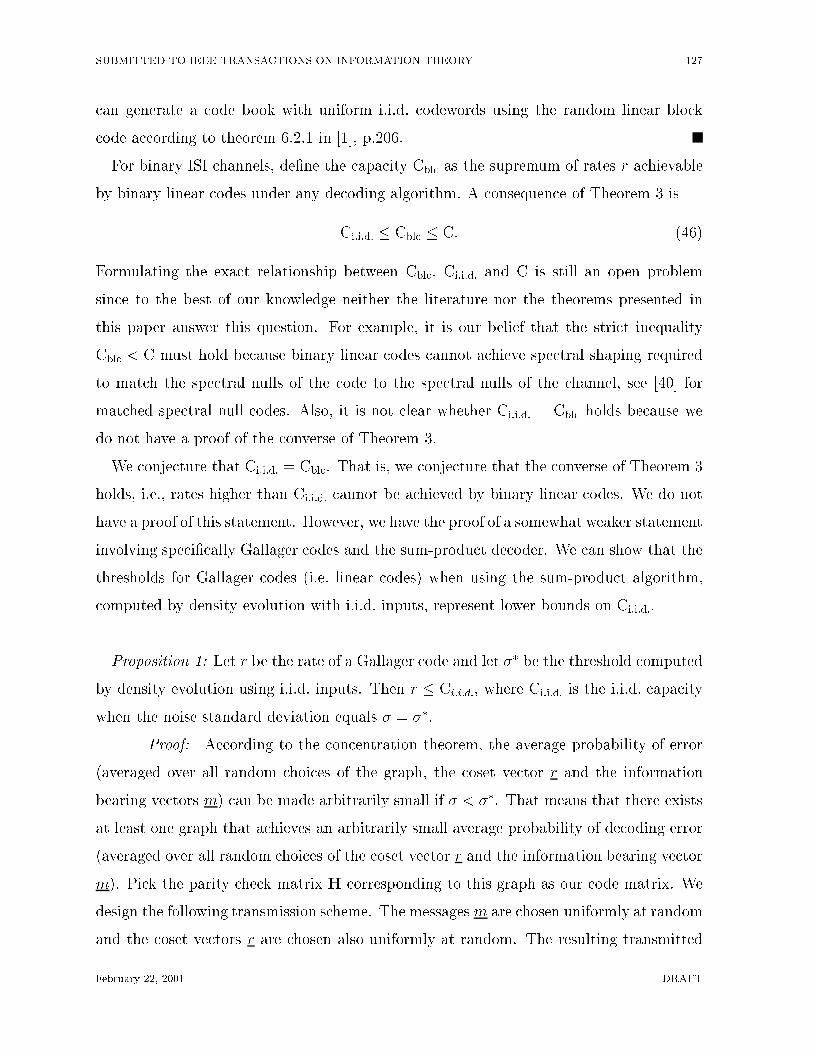
SUBMITTED TO IEEE TRANSACTIONS ON INFORMATION THEORY 127
can generate a code book with uniform i.i.d. codewords using the random linear block
code according to theorem 6.2.1 in [1], p.206.
For binary ISI channels, de�ne the capacity Cblc as the supremum of rates r achievable
by binary linear codes under any decoding algorithm. A consequence of Theorem 3 is
Ci:i:d: � Cblc � C: (46)
Formulating the exact relationship between Cblc, Ci:i:d: and C is still an open problem
since to the best of our knowledge neither the literature nor the theorems presented in
this paper answer this question. For example, it is our belief that the strict inequality
Cblc < C must hold because binary linear codes cannot achieve spectral shaping required
to match the spectral nulls of the code to the spectral nulls of the channel, see [40] for
matched spectral null codes. Also, it is not clear whether Ci:i:d: = Cblc holds because we
do not have a proof of the converse of Theorem 3.
We conjecture that Ci:i:d: = Cblc. That is, we conjecture that the converse of Theorem 3
holds, i.e., rates higher than Ci:i:d: cannot be achieved by binary linear codes. We do not
have a proof of this statement. However, we have the proof of a somewhat weaker statement
involving speci�cally Gallager codes and the sum-product decoder. We can show that the
thresholds for Gallager codes (i.e. linear codes) when using the sum-product algorithm,
computed by density evolution with i.i.d. inputs, represent lower bounds on Ci:i:d:.
Proposition 1: Let r be the rate of a Gallager code and let �� be the threshold computed
by density evolution using i.i.d. inputs. Then r � Ci:i:d:, where Ci:i:d: is the i.i.d. capacity
when the noise standard deviation equals � = ��.
Proof: According to the concentration theorem, the average probability of error
(averaged over all random choices of the graph, the coset vector r and the information
bearing vectors m) can be made arbitrarily small if � < ��. That means that there exists
at least one graph that achieves an arbitrarily small average probability of decoding error
(averaged over all random choices of the coset vector r and the information bearing vector
m). Pick the parity check matrix H corresponding to this graph as our code matrix. We
design the following transmission scheme. The messagesm are chosen uniformly at random
and the coset vectors r are chosen also uniformly at random. The resulting transmitted
February 22, 2001 DRAFT
SUBMITTED TO IEEE TRANSACTIONS ON INFORMATION THEORY 128
sequence is i.i.d. with probability of each symbol 0.5. If the transmitted sequence is i.i.d.,
we cannot �nd a code with rate higher than Ci:i:d: such that the decoding error is arbitrarily
small. But since the decoding error (averaged over all messages m and all cosets r) for
the sum-product decoder of Gallager codes can be made arbitrarily small for � < ��, we
conclude that the code rate r must be smaller than the value for Ci:i:d: evaluated at � < ��.
Therefore r � sup�<��
Ci:i:d:(�) = Ci:i:d:(��).
B. Thresholds for Regular Gallager codes as lower bounds on Ci:i:d:
Due to the two proofs presented in the previous subsection, it follows that the curve
rate (r) vs. threshold (��) for a Gallager code over a binary ISI channel is upper bounded by
the curve Ci:i:d: vs. �. Thus, we have a practical method for numerically lower-bounding
Ci:i:d:. Furthermore, by virtue of specifying the degree polynomials �(x) and �(x), we
also characterize a code that can achieve this lower bound. This is a bounding method
that is di�erent from the closed-form bounds [6], [7] or Monte-Carlo bounds [5] proposed
in the past where no bound-achieving characterization of the code is possible (except
through random coding techniques which are impractical for implementations). Further,
we compare the thresholds obtained by density evolution to the value Ci:i:d: computed by
the Arnold-Loeliger method [8], showing that the thresholds are very close to Ci:i:d: in the
high-code-rate regions (0:7 � r � 1:0). This is exactly the region of practical importance
in storage devices where high-rate codes for binary ISI channels are a necessity [3]. The
codes studied in this paper do not provide tight bounds in the low-rate region, but we
believe that the threshold bounds can be tightened by optimizing the degree polynomials
�(x) and �(x).
In this paper we present thresholds only for regular Gallager codes7 in the family (L;R),
where L = 3 and R is allowed to vary in order to get a variable code rate r = R�3R
. This
family of codes provides a curve r vs. threshold that is very close to Ci:i:d: for high code
rates, but not for low code rates. To get tighter bounds in the low information rate
7Thresholds for irregular Gallager codes can also be obtained via density evolution.
February 22, 2001 DRAFT
SUBMITTED TO IEEE TRANSACTIONS ON INFORMATION THEORY 129
code check-node code rate threshold threshold SNR� [dB]
(L;R) degree R r = R�3R
�� SNR� = 20 log101��
(3,3) 3 0.000 2.042 -6.201
(3,4) 4 0.250 1.196 -1.554
(3,5) 5 0.400 0.945 0.492
(3,6) 6 0.500 0.822 1.703
(3,8) 8 0.625 0.697 3.136
(3,10) 10 0.700 0.631 4.000
(3,15) 15 0.800 0.547 5.241
(3,30) 30 0.900 0.459 6.764
(3,60) 60 0.950 0.404 7.873
(3,150) 150 0.980 0.355 8.996
TABLE I
Thresholds for regular Gallager codes (L = 3); channel h(D) = 1p2� 1p
2D.
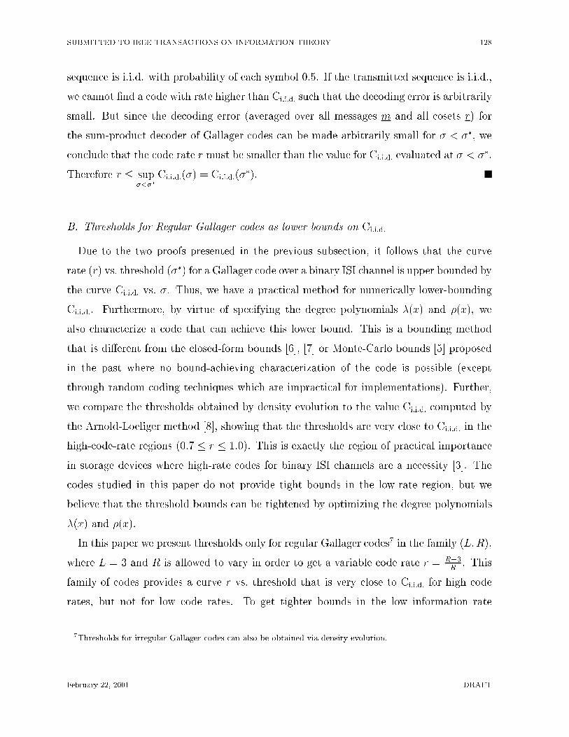
regime, we would have to revert to irregular Gallager codes [9], [10]. Table I tabulates the
codes and their respective thresholds for the ISI channel h(D) = 1p2� 1p
2D with additive
Gaussian noise (this channel was chosen for easy comparison to some previously published
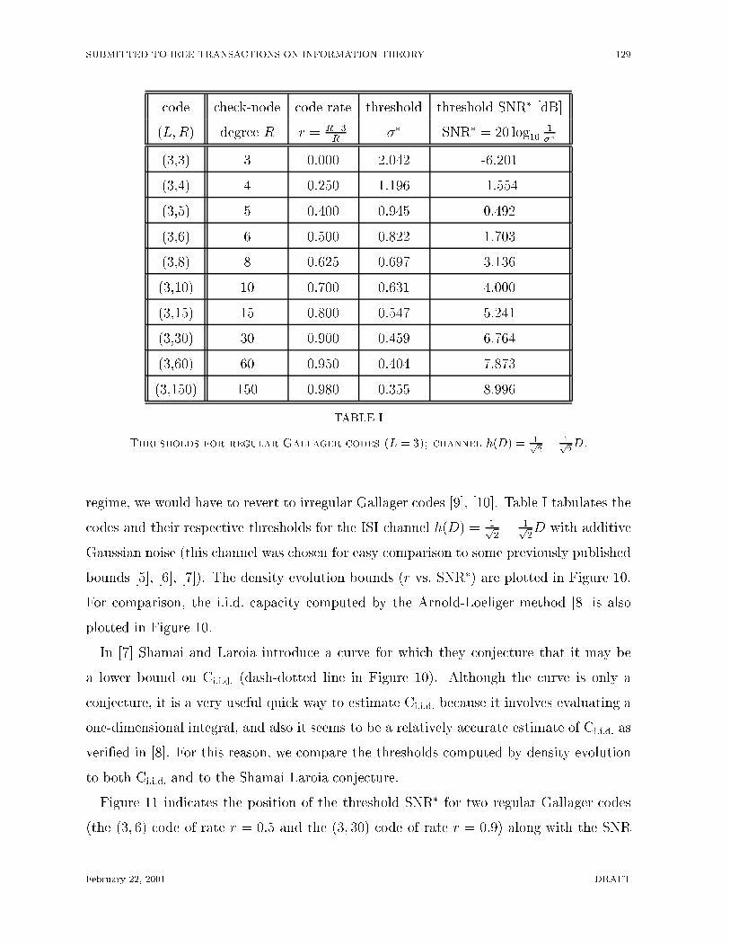
bounds [5], [6], [7]). The density evolution bounds (r vs. SNR�) are plotted in Figure 10.
For comparison, the i.i.d. capacity computed by the Arnold-Loeliger method [8] is also
plotted in Figure 10.
In [7] Shamai and Laroia introduce a curve for which they conjecture that it may be
a lower bound on Ci:i:d: (dash-dotted line in Figure 10). Although the curve is only a
conjecture, it is a very useful quick way to estimate Ci:i:d: because it involves evaluating a
one-dimensional integral, and also it seems to be a relatively accurate estimate of Ci:i:d: as
veri�ed in [8]. For this reason, we compare the thresholds computed by density evolution
to both Ci:i:d: and to the Shamai-Laroia conjecture.
Figure 11 indicates the position of the threshold SNR� for two regular Gallager codes
(the (3; 6) code of rate r = 0:5 and the (3; 30) code of rate r = 0:9) along with the SNR
February 22, 2001 DRAFT
SUBMITTED TO IEEE TRANSACTIONS ON INFORMATION THEORY 130
−8 −6 −4 −2 0 2 4 6 80
0.1
0.2
0.3
0.4
0.5
0.6
0.7
0.8
0.9
1C
i.i.d. and the density evolution threshold
SNR [dB]
Cap
acity
[bits
/cha
nnel
−us
e]
(3,4) regular Gallager code
(3,5) regular Gallager code
(3,6) regular Gallager code
(3,8) regular code
(3,10) regular code
(3,15) code
(3,30)(3,60)
(3,150)
Ci.i.d.
density evolution threshold
(3,3) regular Gallager code
Fig. 10. The i.i.d. capacity Ci:i:d: and thresholds for regular Gallager codes with message node degree
L = 3.
0.6 0.8 1 1.2 1.4 1.6 1.8 2 2.210
−5
10−4
10−3
Bit error rates and SNRs for (3,6) codes (rate r=0.5)
SNR [dB]
BIT
ER
RO
R R
AT
E
SNR*SNR for the Shamai−Laroia conjecture
SNR for C
i.i.d.
n=106
n=105
n=104
6.4 6.5 6.6 6.7 6.8 6.9 7 7.1 7.210
−5
10−4
10−3
Bit error rates and computed SNRs for (3,30) codes (rate r=0.9)
SNR [dB]
BIT
ER
RO
R R
AT
E
SNR*SNR for the Shamai−Laroia conjecture
SNR for Ci.i.d.
n=106 n=105n=104
Fig. 11. Comparison of bit error simulation results for �nite-block-length Gallager codes of rates r = 0:5
and r = 0:9 to Ci:i:d: and to the density evolution thresholds and to the Shamai-Laroia conjectured
bound.
values for the Shamai-Laroia conjecture at these rates and the best known value for Ci:i:d:
computed by the Arnold-Loeliger method [8]. Also shown in Figure 11 are the SNR values
for which simulated Gallager codes of lengths n 2 f104; 105; 106g achieved bit error rates of
10�5. First, observe that the thresholds accurately predict the limit of code performance
as the block length n becomes very large. Next, observe that for the code (3; 30) of rate
r = 0:9, the threshold is tight (tighter than the Shamai-Laroia conjecture), establishing
that regular Gallager codes are relatively good codes for high rates. For the code (3; 6)
February 22, 2001 DRAFT
SUBMITTED TO IEEE TRANSACTIONS ON INFORMATION THEORY 131
of rate r = 0:5, the threshold is far away from the SNR values corresponding to Ci:i:d:
and the Shamai-Laroia conjecture, respectively, suggesting that good Gallager codes in
the low-rate regime should be sought among irregular codes [9].
C. The BCJR-once bound
Due to the high computational complexity of the BCJR (forward-backward) algorithm,
several authors suggest applying the BCJR step only once [29], [41] and subsequently
iterating the message-passing decoding algorithm only within the code subgraph of the
joint channel/code graph (see Figure 3). Clearly, this strategy is suboptimal to fully
iterating between the channel and the code subgraphs of the joint channel/code graph,
but does provide substantial computational savings, which is of particular importance for
on-chip implementations. The question that remains is how much does one lose in terms
of achievable information rate when this strategy is applied. We develop next what we
call the BCJR-once bound CBCJR�once which answers this question.
Let xn1 be a realization of a random channel input sequence Xn1 . Let y
n1be a realization
of the channel output sequence Y n1 . Let Ot = O(0)t be the message passed from the t-th
trellis node to the variable node in the �rst round of the sum-product algorithm (i.e., it is
the output of the BJCR algorithm applied once in the �rst iteration of decoding). Denote
the vector of realizations O1; :::; On by On1 , which is a realization of a random vector On1 .
We assume that the input sequence is i.i.d., and de�ne the BCJR-once bound as
CBCJR�once = limn!1
1
nsup
Pr(Xn1=x
n1 )=
nQ
t=1Pr(X=xt)
nXt=1
I (Xt;Ot) : (47)
For the channel in (1) with binary inputs, due to the channel symmetry, the supremum
in (47) is achieved when Pr (X = 1) = 12.
Two straight-forward properties can be established for the BCJR-once bound.
Property 1: CBCJR�once = limn!1
1n
sup
Pr(Xn1=x
n1 )=
nQ
t=1Pr(X=xt)
nPt=1
I (Xt;Yn1 ).
Proof: The BCJR algorithm computes Ot = lnPr(Xt=1jY n
1=yn1 )
1�Pr(Xt=1jY n1=y
n1 ). So, Ot is a suÆcient
statistic for determiningXt from Y n1 . Therefore (see e.g. [2], p. 37), I (Xt;Y
n1 ) = I (Xt;Ot).
February 22, 2001 DRAFT
SUBMITTED TO IEEE TRANSACTIONS ON INFORMATION THEORY 132
Property 2: CBCJR�once � Ci:i:d:.
Proof: Let H (Xn1 jY
n1 ) denote the conditional entropy of Xn
1 given Y n1 , and let
H (Xt) denote the entropy of Xt. From the independence bound ([2], p. 28) it follows that
H (Xn1 jY
n1 ) �
nPt=1
H (XtjYn1 ). If X
n1 is a vector of i.i.d. random variables, we have
I (Xn1 ;Y
n1) =
nXt=1
H (Xt)�H (Xn1 jY
n1 )
�nXt=1
[H (Xt)�H (XtjYn1)]
=nXt=1
I (Xt;Yn1 ) (48)
Using Property 1, the supremum of the right-hand side of (48) is CBCJR�once, in the limit
n!1, and the supremum of the left-hand side is Ci:i:d:.
The BCJR-once bound also has another very important property, which we state very
loosely. Let us consider the inputs Xt and the BCJR-once outputs Ot as a communications
channel. If we disregard the channel memory of the channel Xt ! Ot, then there does not
exist a code of rate r > CBCJR�once for which the decoding error can be made arbitrarily
small. Of course, this statement is not very rigorous unless we use a very precise de�nition
of the phrase \disregard the channel memory", which we will not do here. Instead, in
subsection V-D we give a precise statement involving Gallager codes: we show that the
rate of a Gallager code plotted against the BCJR-once threshold (computed for the same
Gallager code using density-evolution for the BCJR-once sum-product algorithm), must
be lower than CBCJR�once evaluated at the same SNR.
The BCJR-once bound CBCJR�once for the channel in (1) can be computed by i) running
the BJCR algorithm on a very long trellis section, ii) collecting the outputs, iii) quantizing
them, iv) forming a histogram for the symbol-to-symbol transition probabilities, and v)
computing the mutual information of a memoryless channel whose transition probabilities
equal to those computed by the histogram. Another way is to devise a method similar
to the Arnold-Loeliger method for computing Ci:i:d: (see [8]). First, we note that the
bound achieving i.i.d. input distribution is the one with equally likely symbols, yielding
1nH (Xn
1 ) = 1. Thus, the problem of computing CBCJR�once reduces to the problem of
February 22, 2001 DRAFT
SUBMITTED TO IEEE TRANSACTIONS ON INFORMATION THEORY 133
computing
limn!1
1
n
nXt=1
H (XtjYn1 ) = lim
n!11
n
nXt=1
E
24� X
Xt2f�1;1gPr (Xt = xtjY
n1 ) log2 Pr (Xt = xtjY
n1 )
35
= limn!1
1
n
nXt=1
E [H (Pr (Xt = 1jY n1 ))] ; (49)
where H(p) is the binary entropy function de�ned as H(p) = �p log2 p�(1�p) log2(1�p).
For a given channel output realization yn1, the sum-product (BCJR/Baum-Welch/forward-
backward) algorithm computes Pr�Xt = 1jyn
1
�. So, we can estimate (49) by generating an
n-long i.i.d. input sequence, transmitting it over the channels and running the BCJR algo-
rithm (sum-product algorithm) on the observed channel output yn1to get Pr
�Xt = 1jyn
1
�for every 1 � t � n. The estimate
1
n
nXt=1
H�Pr�Xt = 1jyn
1
��
converges in probability to (49) as n!1.
The BCJR-once bound CBCJR�once (computed in the manner described above for n =
106) is depicted as the dashed curve in Figure 12 (the same �gure also shows three other
curves: 1) the curve for Ci:i:d: as computed by the Arnold-Loeliger method, 2) the thresh-
olds presented in subsection V-B and 3) the BCJR-once thresholds for regular Gallager
codes which are presented next in subsection V-D).
D. BCJR-once thresholds for regular Gallager codes
Just as we performed density evolution for the full sum-product algorithm over the joint
channel/code graph, we do the same for the BCJR-once version of the decoding algorithm.
The only di�erence here is in the shape of the depth-` message ow neighborhood, while
the general method remains the same. Denote by ��BCJR�once the noise tolerance threshold
for the BCJR-once sum-product algorithm for a Gallager-code/ISI-channel combination.
The threshold ��BCJR�once can be computed by density evolution on a tree-like message ow
neighborhood assuming that the trellis portion of the sum-product algorithm is executed
only in the �rst decoding round.
February 22, 2001 DRAFT
SUBMITTED TO IEEE TRANSACTIONS ON INFORMATION THEORY 134
Proposition 2: Let r be the rate of a Gallager code and let ��BCJR�once be the BCJR-
once noise tolerance threshold (computed by density evolution using i.i.d. inputs). Then
r � CBCJR�once, where CBCJR�once is the BCJR-once bound evaluated at the noise standard
deviation � = ��BCJR�once.
Proof: The threshold ��BCJR�once is computed using the density evolution method
described in Section IV-A where the trellis evolution step is executed only in the �rst
round. Thus, the threshold ��BCJR�once is computed as the threshold of a Gallager code
of rate r on a memoryless channel, whose channel law (conditional pdf of channel output
given the channel input) is given by
fOtjXt (OtjXt = 1) = limW!1
fO[W ]t jXt
(OtjXt = 1) ;
where O[W ]t is the output of the windowed BCJR algorithm when the window size is W ,
and clearly, due to the channel symmetry fOtjXt (OtjXt = �1) = fOtjXt (�OtjXt = 1). As
evident from the density averaging in the trellis portion of the density evolution, the func-
tion fO[W ]t jXt
(OtjXt = 1) is the average conditional pdf of O[W ]t , taken over all conditional
pdf's of O[W ]t conditioned on Xt+W
t�W�I under the constraint Xt = 1, i.e.
fO[W ]t jXt
�O[W ]t jXt = 1
�= 2�(2W+I) �
Xall xt�Wt�W�I ; xt=1
fO[W ]t jXt+W
t�W�I
�OtjXt+W
t�W�I = xt�Wt�W�I�:
For this memoryless channel, the channel capacity is C+ = limW!1
I�Xt;O
[W ]t
�. Since
the decoder achieves an arbitrarily small probability of error for all � � ��, due to the
concentration theorem for memoryless channels [20], it follows that r � sup����BCJR�once
C+(�) =
C+(�BCJR�once). The proof is completed by noticing that C+ = CBCJR�once as de�ned
in (47).
Again, we choose the family of regular Gallager codes with a constant check node degree
L = 3 and a varying variable node degree R. The channel is h(D) = 1p2� 1p
2D with
additive white Gaussian noise. The BCJR-once thresholds are given in Table II, and the
corresponding plot is given in Figure 12. Figure 12 shows the BCJR-once bound derived
in subsection V-C. It can be seen that the regular Gallager codes have the capability to
February 22, 2001 DRAFT
SUBMITTED TO IEEE TRANSACTIONS ON INFORMATION THEORY 135
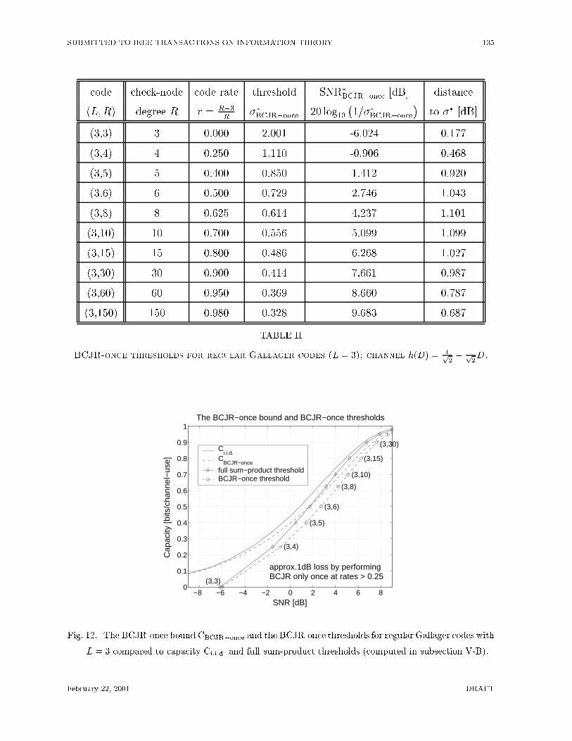
code check-node code rate threshold SNR�BCJR�once [dB] distance
(L;R) degree R r = R�3R
��BCJR�once 20 log10�1=��BCJR�once
�to �� [dB]
(3,3) 3 0.000 2.001 -6.024 0.177
(3,4) 4 0.250 1.110 -0.906 0.468
(3,5) 5 0.400 0.850 1.412 0.920
(3,6) 6 0.500 0.729 2.746 1.043
(3,8) 8 0.625 0.614 4.237 1.101
(3,10) 10 0.700 0.556 5.099 1.099
(3,15) 15 0.800 0.486 6.268 1.027
(3,30) 30 0.900 0.414 7.661 0.987
(3,60) 60 0.950 0.369 8.660 0.787
(3,150) 150 0.980 0.328 9.683 0.687
TABLE II
BCJR-once thresholds for regular Gallager codes (L = 3); channel h(D) = 1p2� 1p
2D.
−8 −6 −4 −2 0 2 4 6 80
0.1
0.2
0.3
0.4
0.5
0.6
0.7
0.8
0.9
1The BCJR−once bound and BCJR−once thresholds
SNR [dB]
Cap
acity
[bits
/cha
nnel
−us
e]
approx.1dB loss by performing BCJR only once at rates > 0.25
(3,3)
(3,4)
(3,5)
(3,6)
(3,8)
(3,10)
(3,15)
(3,30)C
i.i.d.
CBCJR−once
full sum−product thresholdBCJR−once threshold
Fig. 12. The BCJR-once bound CBCJR�once and the BCJR-once thresholds for regular Gallager codes with
L = 3 compared to capacity Ci:i:d: and full sum-product thresholds (computed in subsection V-B).
February 22, 2001 DRAFT
SUBMITTED TO IEEE TRANSACTIONS ON INFORMATION THEORY 136
achieve the BCJR-once bound at high information rates if the BCJR-once version of the
message-passing decoding algorithm is applied. For comparison, Figure 12 also shows the
curve for Ci:i:d: as computed by the Arnold-Loeliger method [8]. It can be seen that the
BCJR-once bound is very close to Ci:i:d: at low SNRs, but is about 1 dB away from Ci:i:d: at
higher information rates. The di�erence between the full sum-product threshold curve and
the BCJR-once threshold curve also seems to be closely approximated by the di�erence
between Ci:i:d: and CBCJR�once. We thus conclude that, say at rate r = 0:9, we can expect
to see a loss of 1 dB if we execute the BCJR algorithm only once at the very beginning
of the sum-product decoding algorithm (as opposed to executing the trellis sum-product
algorithm in every iteration of the decoder).
VI. Conclusion
In this paper we have developed a density evolution method for determining the asymp-
totic performance of Gallager codes over binary ISI channels in the limit n!1, where n
is the block length. We proved two concentration theorems 1) for concentration for a par-
ticular transmitted sequence and 2) for a random transmitted sequence of i.i.d. symbols.
The noise tolerance threshold was de�ned as the supremum of noise standard deviations
for which the probability of decoding error tends to zero as the number of rounds of the
decoding algorithm tends to in�nity. We also established that the code rate r vs. the noise
tolerance threshold establishes a curve that is upper bounded by the i.i.d. capacity of bi-
nary ISI channels. We have computed the thresholds for regular Gallager codes with three
ones per column of the parity check matrix over the dicode channel (h(D) = 1p2� 1p
2D)
and showed that they get very close to the limit of i.i.d. capacity in the high code rate
region. For low code rates, regular Gallager codes do not perform close to the capacity.
A good low-rate code should therefore be sought in the space of irregular Gallager codes.
We also showed via Monte Carlo simulations that codes with increasing code lengths n
approach closely the threshold computed by density evolution.
We also explored the limits of performance of Gallager codes if a slightly more practical
sum-product algorithm is utilized. Since the computational bottleneck in the sum-product
algorithm for ISI channels is the trellis portion of the algorithm, it is computationally
February 22, 2001 DRAFT
SUBMITTED TO IEEE TRANSACTIONS ON INFORMATION THEORY 137
advantageous to run the trellis portion of the algorithm only once at the beginning of the
�rst decoding iteration, i.e. the \BCJR-once" version of the algorithm. This algorithm
su�ers from a performance loss compared to the full sum-product algorithm. We computed
the maximal achievable rate of the BCJR-once sum-product algorithm and showed that for
the dicode channel (h(D) = 1p2� 1p
2D), the asymptotic performance loss at high rates is
about 1 dB, while for low rates the loss is minimal. Approximately, the same di�erence (at
most 1.1 dB) was observed for the thresholds computed for the full sum-product algorithm
and the BCJR-once version.
We conclude the paper by pointing out some remaining challenges in coding for binary
ISI channels. While the computation of Ci:i:d: is now solved [8], the computation of the
capacity remains a challenge. A method for lower-bounding C by extending the memory
of the source is presented in [8], suggesting that at high rates C and Ci:i:d: are close to each
other (at low rates C and Ci:i:d: di�er substantially). In channels of practical interest, i.e.,
channels with signal-dependent noise [42], due to the signal-dependent nature of the noise
C and Ci:i:d: may not be close to each other even in the high rate region. There is a need
for a practical tool for computing the lower bound on C by optimizing the trellis transition
probabilities of an extended-memory source [8]. Another challenging problem is to move
the performance thresholds of practical codes beyond Ci:i:d:. A viable strategy may be to
somehow combine the bene�cial spectral-shaping characteristics of matched spectral null
codes [40] with Gallager's low density parity check constraints, but it is not clear how
to achieve this and still have a relatively simple encoder/decoder. Even for linear binary
codes (i.e., non-spectral-shaping codes) the optimization of irregular Gallager codes to
achieve Ci:i:d: is also a challenging problem.
Appendix
We brie y describe the windowed BCJR algorithm mainly for completeness of the text.
Our description uses a compact matrix notation. For a conventional description, we refer
the reader to [25]. The notation in this appendix refers to Figure 4. We start with the
messages e(`)t available from the code portion of the graph and yt available from the channel
February 22, 2001 DRAFT
SUBMITTED TO IEEE TRANSACTIONS ON INFORMATION THEORY 138
output, where 1 � t � n, and n is the codeword length. First set
P(`)1;t =
exphe(`)t
i1 + exp
he(`)t
iP(`)�1;t = 1� P
(`)1;t :
(50)
Then for every t form a diagonal matrix D(`)t of size 2I � 2I , where I is the ISI length of
the channel. Enumerate the states of the �nite state machine with numbers 1 through 2I .
Set the i-th diagonal element of D(`)t as
D(`)t (i; i) =
8<: P
(`)�1;t if i�th state is reached when the channel input at time t is�1:
P (`)1;t if i�th state is reached when the channel input at time t is 1:
:
Next, for every t form a matrix Tt of size 2I � 2I , with the entry in the intersection of the
i-th row and j-th column given by
Tt(i; j) =
8>><>>:
0 if no trellis branch leads from state i to state j:
exp
"�(yt � �[i; j])2
2�2
#otherwise
;
where �[i; j] is the noiseless channel output when the �nite-state machine corresponding
to the ISI channel transitions from state i to state j. Now, for each t form the two vectors
of size 2I � 1
�(`)W;t =
�2�I; 2�I ; � � � ; 2�I
�T�(`)W;t
=�2�I; 2�I ; � � � ; 2�I
�T:
For every t, compute
�(`)0;t =
�D
(`)t�1Tt�1
��D
(`)t�2Tt�2
�� � ��D
(`)t�WTt�W
��(`)W;t (51)
�(`)0;t
=�D
(`)t+1Tt+1
�T �D
(`)t+2Tt+2
�T� � ��D
(`)t+WTt+W
�T�(`)W;t
: (52)
For each t compute the vector b(`)t as
b(`)t = �(`)
0;t��Tt � �
(`)0;t
�; (53)
February 22, 2001 DRAFT
SUBMITTED TO IEEE TRANSACTIONS ON INFORMATION THEORY 139
where � denotes the Hadamard (i.e., element-wise) product of two vectors. Denote byP�1
b(`)t the sum of the elements of b
(`)t that correspond to the states that are reached if the
channel input is �1, i.e., the element b(`)t (i) is included in the sum if state i is reached
when the channel input is �1. Similarly, denote byP1
b(`)t the sum of the elements of b
(`)t
that correspond to the states that are reached if the channel input is 1. Then the message
to the code portion of the graph is computed as
O(`)t = ln
P1
b(`)tP�1
b(`)t
:
The windowed BCJR algorithm described in this Appendix is not the most economical
method (in terms of memory). Our aim was to give a compact description for completeness
of the text. In practice, to achieve a numerically stable method, the multiplications in (51)
and (52) need to be normalized such that the vector obtained by successive multiplication
from the left all have the property that the sum of their elements equal to 1 [25]. For
other implementations of the windowed BCJR algorithm, see [43], [44], [45].
Acknowledgments
The authors would like to thank Sae-Young Chung for extremely helpful discussions on
implementations of the density evolution algorithm, Dieter Arnold for providing the latest
results on capacity computations even before they appeared in print and Xiaowei Jin and
Nedeljko Varnica for helping with the simulations of Gallager codes of �nite block lengths.
References
[1] R. G. Gallager, Information Theory and Reliable Communication. New York: John Wiley and Sons, Inc.,
1968.
[2] T. M. Cover and J. A. Thomas, Elements of Information Theory. New York: John Wiley and Sons, 1991.
[3] K. A. S. Immink, P. H. Siegel, and J. K. Wolf, \Codes for digital recorders," IEEE Trans. Inform. Theory,
vol. 44, pp. 2260{2299, October 1998.
[4] J. G. Proakis, Digital Communications. New York: McGraw-Hill, 4th ed., 2000.
[5] W. Hirt, Capacity and Information Rates of Discrete-Time Channels with Memory. PhD thesis, Swiss Federal
Institute of Technology (ETH), Zurich, Switzerland, 1988.
[6] S. Shamai (Shitz), L. H. Ozarow, and A. D. Wyner, \Information rates for a discrete-time Gaussian channel
with intersymbol interference and stationary inputs," IEEE Transactions on Information Theory, vol. 37,
pp. 1527{1539, 1991.
February 22, 2001 DRAFT
SUBMITTED TO IEEE TRANSACTIONS ON INFORMATION THEORY 140
[7] S. Shamai (Shitz) and R. Laroia, \The intersymbol interference channel: Lower bounds on capacity and
channel precoding loss," IEEE Transactions on Information Theory, vol. 42, pp. 1388{1404, 1996.
[8] D. Arnold and H.-A. Loeliger, \On the information rate of binary-input channels with memory," in Proc. IEEE
ICC 2001, (Helsinki), pp. ?{?, June 2001.
[9] M. Luby, M. Mitzenmacher, M. A. Shokrollahi, and D. Spielman, \Analysis of low density codes and improved
designs using irregular graphs," to appear in IEEE Trans. Inform. Theory, vol. ?, pp. ?{?, 2001. also in
Proceedings of the 30th Annual ACM Symposium on Theory of Computing, pages 249{258, 1998.
[10] T. Richardson, A. Shokrollahi, and R. Urbanke, \Design of capacity-approaching low-density parity-
check codes," to appear in IEEE Trans. Inform. Theory, vol. ?, pp. ?{?, 2001. available at
http://lcavwww.ep .ch/ ruediger/publications.html.
[11] R. G. Gallager, Low-Density Parity-Check Codes. Cambridge, MA: MIT Press, 1962.
[12] B. M. Tanner, \A recursive approach to low complexity codes," IEEE Trans. Inform. Theory, vol. 27, pp. 533{
547, September 1981.
[13] N. Wiberg, H.-A. Loeliger, and R. K�otter, \Codes and iterative decoding on general graphs," Eoropean
Trans. on Commun., vol. 6, pp. 513{526, September 1995.
[14] G. D. Forney Jr., \Codes on graphs: Normal realizations," to appear in IEEE Trans. Inform. Theory, vol. 47,
pp. ?{?, February 2001.
[15] D. J. C. MacKay and R. M. Neal, \Near Shannon limit performance of low-density parity-check codes,"
Electronic Letters, vol. 32, pp. 1645{1646, 1996.
[16] D. J. C. MacKay, \Good error-correcting codes based on very sparce matrices," IEEE Trans. Inform. Theory,
vol. 45, pp. 399{431, March 1999.
[17] C. Berrou, A. Glavieux, and P. Thitimajshima, \Near Shannon limit error-correcting coding and decoding:
Turbo-codes," in Proc. IEEE Int. Conf. on Communications, (Geneva, Switzerland), pp. 1064{1070, May
1993.
[18] M. G. Luby, M. Mitzenmacher, M. A. Shokrollahi, and D. A. Spielman, \Improved low density parity check
codes using irregular graphs and belief propagation," in Proc. IEEE Int. Symp. Inform. Theory, (Cambrdge,
MA), p. 117, Aug. 1998.
[19] M. Luby, M. Mitzenmacher, and M. A. Shokrollahi, \Analysis of random processes via and-or tree evaluation,"
in Proceedings of the 9th Annual ACM-SIAM Symposium on Discrete Algorithms, pp. 364{373, 1998.
[20] T. Richardson and R. Urbanke, \The capacity of low-density parity check codes under message-
passing decoding," to appear in IEEE Trans. Inform. Theory, vol. ?, pp. ?{?, 2001. available at
http://lcavwww.ep .ch/ ruediger/publications.html.
[21] T. Richardson and R. Urbanke, \Thresholds for turbo codes," in Proc. IEEE Int. Symp. Inform. Theory,
(Sorrento, Italy), p. 317, June 2000.
[22] S.-Y. Chung, G. D. Forney, T. Richardson, and R. Urbanke, \On the design of low-density parity-check codes
within 0.0045 dB of the Shannon limit." accepted for publication in IEEE Communications Letters; available
at http://lcavwww.ep .ch/ ruediger/publications.html., 2000.
[23] F. R. Kschischang, B. J. Frey, and H.-A. Loeliger, \Factor graphs and the sum-product algorithm." submitted
for publication in IEEE Trans. Inform. Theory; available at http://citeseer.nj.nec.com/cachedpage/13132,
1998.
[24] G. D. Forney Jr., \Maximum-likelihood sequence estimation of digital sequences in the presence of intersymbol
interference," IEEE Transactions on Information Theory, vol. 18, pp. 363{378, March 1972.
February 22, 2001 DRAFT
SUBMITTED TO IEEE TRANSACTIONS ON INFORMATION THEORY 141
[25] L. R. Bahl, J. Cocke, F. Jelinek, and J. Raviv, \Optimal decoding of linear codes for minimizing symbol error
rate," IEEE Trans. Inform. Theory, vol. 20, pp. 284{287, Sept. 1974.
[26] J. Hagenauer and P. Hoeher, \A Viterbi algorithm with soft-decision outputs and its applications," in
Proc. IEEE Global Telecommunications Conference, (Dallas, TX), pp. 1680{1686, November 1989.
[27] Y. Li, B. Vucetic, and Y. Sato, \Optimum soft-output detection for channels with intersymbol interference,"
IEEE Trans. Inform. Theory, vol. 41, pp. 704{713, May 1995.
[28] M. P. C. Fossorier, F. Burkert, S. Lin, and J. Hagenauer, \On the equivalence between SOVA and max-log-
MAP decodings," IEEE Communications Letters, vol. 2, pp. 137{139, May 1998.
[29] Z.-N. Wu and J. M. CioÆ, \Low complexity iterative decoding with decision aided equalization for magnetic
recording channels." to appear in IEEE Journal on Selected Areas in Communications, March issue, 2001.
[30] M. T�uchler, R. K�otter, and A. Singer, \Iterative correction of ISI via equalization and decoding with priors,"
in Proc. IEEE Int. Symp. Inform. Theory, (Sorrento, Italy), p. 100, June 2000.
[31] J. Pearl, Probabilistic Reasoning and Intelligent Systems. San Mateo, CA: Morgan Kaufmann, 1988.
[32] R. J. McEliece, D. J. C. MacKay, and J.-F. Cheng, \Turbo decoding as an instance of Pearl's belief propagation
algorithm," IEEE Journal on Selected Areas in Communications, vol. 16, pp. 140{152, February 1998.
[33] J. Douillard, M. Jezequel, C. Berrou, A. Picart, P. Didier, and A. Glavieux, \Iterative correction of intersymbol
interference: Turbo-equalization," Eoropean Trans. on Commun., vol. 6, pp. 507{511, September 1995.
[34] J. Fan, A. Friedmann, E. Kurtas, and S. McLaughlin, \Low density parity check codes for magnetic recording,"
in Proc. Allerton Conference on Communications and Control, 1999.
[35] S.-Y. Chung, T. Richardson, and R. Urbanke, \Analysis of sum-product decoding of low-density parity-check
codes using gaussian approximation." submitted for publication in IEEE Trans. Inform. Theory; available at
http://lcavwww.ep .ch/ ruediger/publications.html., 2000.
[36] D. J. C. MacKay, \Gallager codes - recent results." available at http://wol.ra.phy.cam.ac.uk/.
[37] R. Motwani and P. Raghavan, Randomized Algorithms. Cambridge: Cambridge University Press, 1995.
[38] A. V. Oppenheim and R. W. Schafer, Discrete-Tiem Signal Processing. Englewoods Cli�s, NJ: Prentice Hall,
1989.
[39] A. Lapidoth and E. I. Teatar, \The compound channel capacity of a class of �nite-state channels," IEEE
Trans. Inform. Theory, vol. 44, pp. 973{983, May 1998.
[40] R. Karabed and P. H. Siegel, \Matched spectral-null codes for partial response channels," IEEE Trans. In-
form. Theory, vol. 37, pp. 818{855, May 1991.
[41] T. Souvignier, A. Friedmann, M. �Oberg, P. Siegel, R. E. Swanson, and J. K. Wolf, \Turbo codes for PR4:
Parallel versus seral concatenation," in Proc. IEEE Int. Conf. on Communications, (Vancouver, Canada),
pp. 1638{1642, June 1999.
[42] A. Kav�ci�c and M. Srinivasan, \The minimum description length principle for modeling recording channels."
submitted for publication in IEEE Journal on Selected Areas in Communications, March issue, 2001.
[43] S. Benedetto, D. D., M. G., and P. F., \Algorithm for continuous decoding of turbo codes," Electronics
Letters, vol. 32, pp. 314{315, February 1996.
[44] A. Viterbi, \An intuitive justi�cation and a simpli�ed implementation of the MAP decoder for convolutional
codes," IEEE Journal on Selected Areas in Communications, vol. 16, pp. 260{264, February 1998.
[45] B. Bai, M. X., and X. Wang, \Novel algorithm for continuous decoding of turbo codes," IEE Proc. Commun.,
vol. 46, pp. 314{315, October 1999.
February 22, 2001 DRAFT


