59
Search Trees Chapter 11 6 9 2 4 1 8 < > =
Search Trees
Chapter 11
6
92
41 8
<
>
=
Outline
Binary Search Trees
AVL Trees
Splay Trees
Outline
Binary Search Trees
AVL Trees
Splay Trees
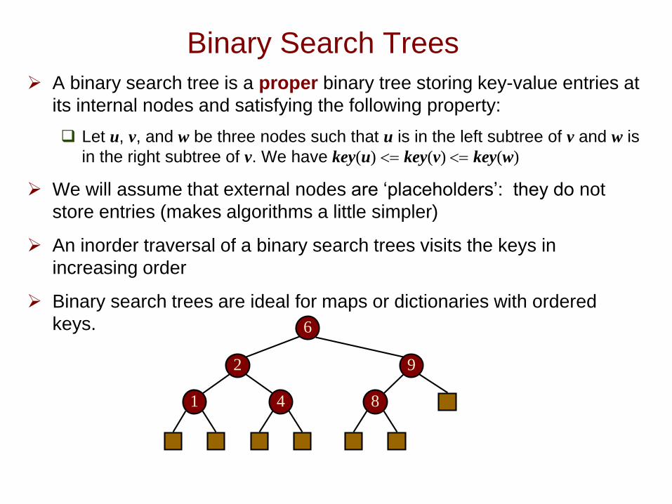
Binary Search Trees
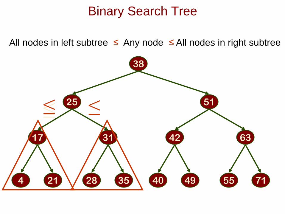
A binary search tree is a proper binary tree storing key-value entries at
its internal nodes and satisfying the following property:
Let u, v, and w be three nodes such that u is in the left subtree of v and w is
in the right subtree of v. We have key(u) <= key(v) <= key(w)
We will assume that external nodes are ‘placeholders’: they do not
store entries (makes algorithms a little simpler)
An inorder traversal of a binary search trees visits the keys in
increasing order
Binary search trees are ideal for maps or dictionaries with ordered
keys. 6
92
41 8
38
25
17
4 21
31
28 35
51
42
40 49
63
55 71
Binary Search Tree
All nodes in left subtree ≤ Any node ≤ All nodes in right subtree
≤≤ ≤
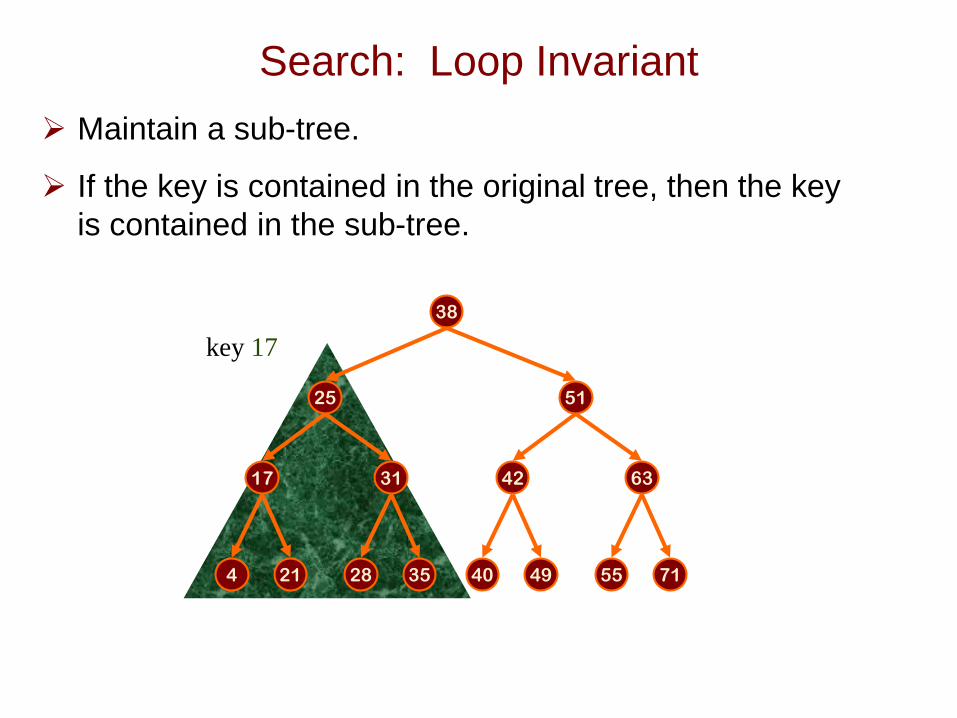
Search: Loop Invariant
Maintain a sub-tree.
If the key is contained in the original tree, then the key
is contained in the sub-tree.
key 17
38
25
17
4 21
31
28 35
51
42
40 49
63
55 71
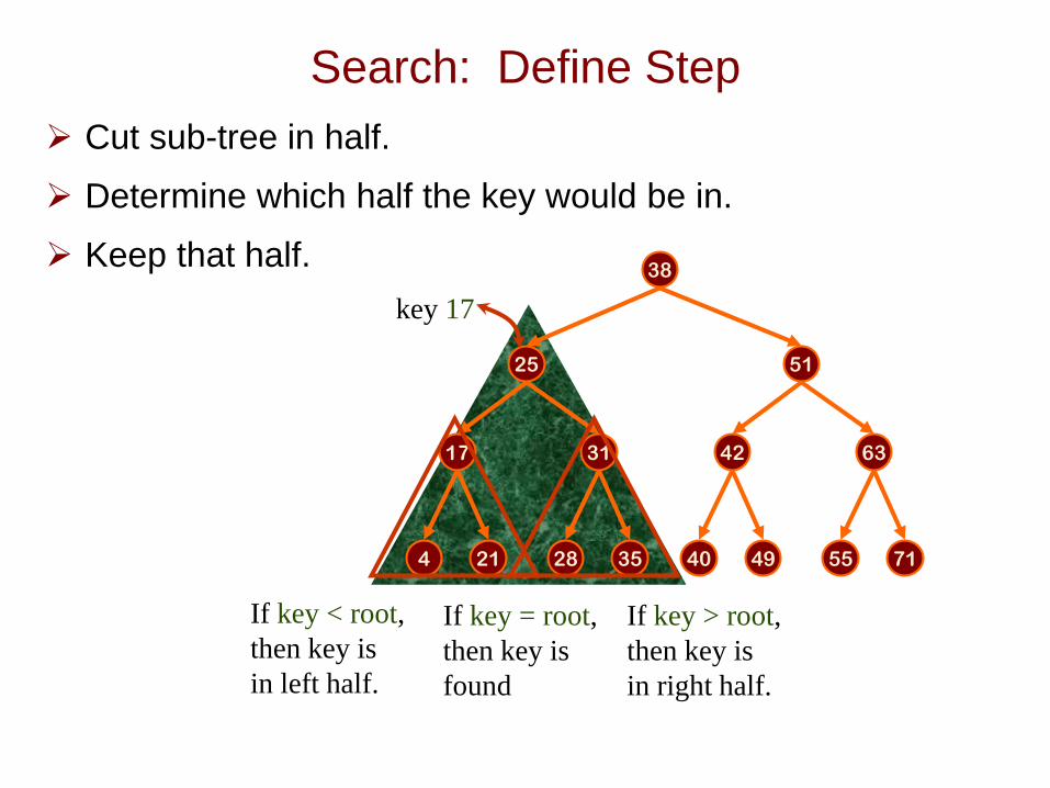
Search: Define Step
Cut sub-tree in half.
Determine which half the key would be in.
Keep that half.
key 17
38
25
17
4 21
31
28 35
51
42
40 49
63
55 71
If key < root,
then key is
in left half.
If key > root,
then key is
in right half.
If key = root,
then key is
found
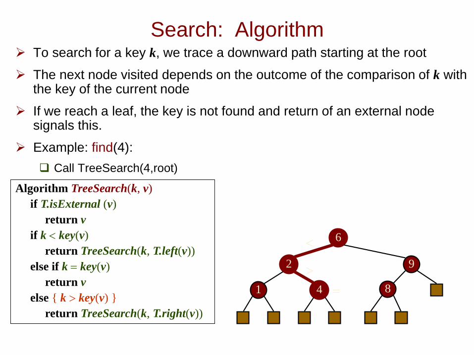
Search: Algorithm To search for a key k, we trace a downward path starting at the root
The next node visited depends on the outcome of the comparison of k with the key of the current node
If we reach a leaf, the key is not found and return of an external node signals this.
Example: find(4):
Call TreeSearch(4,root)
Algorithm TreeSearch(k, v)
if T.isExternal (v)
return v
if k < key(v)
return TreeSearch(k, T.left(v))
else if k = key(v)
return v
else { k > key(v) }
return TreeSearch(k, T.right(v))
6
92
41 8
<
>
=
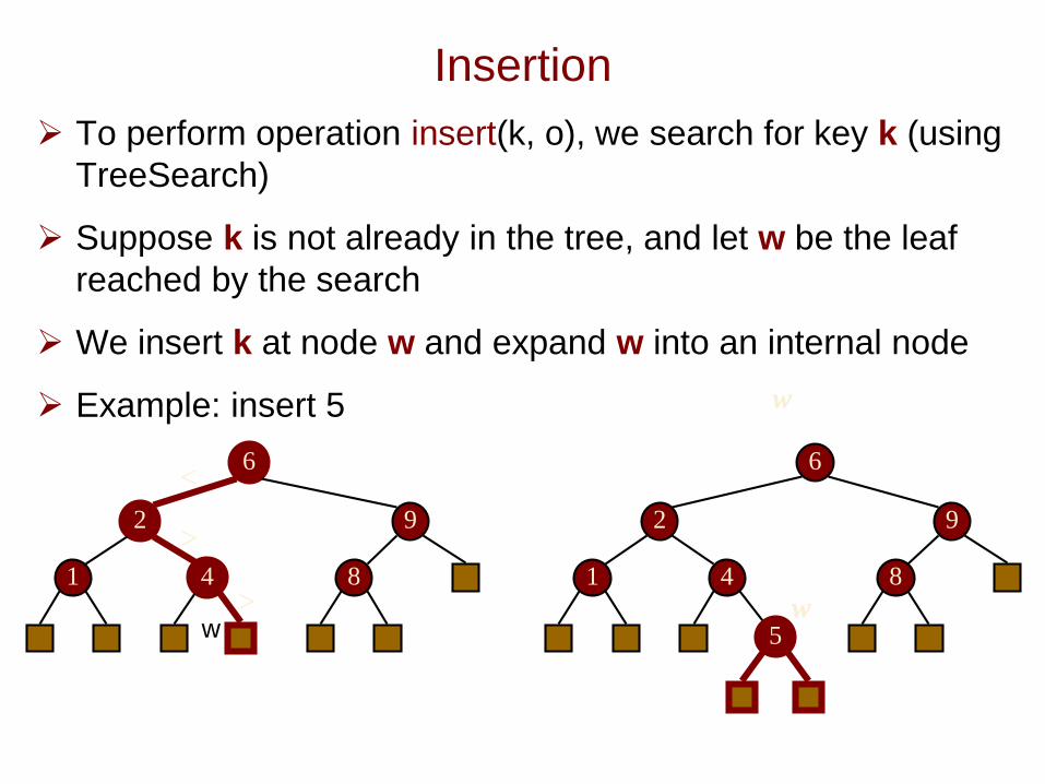
Insertion
To perform operation insert(k, o), we search for key k (using
TreeSearch)
Suppose k is not already in the tree, and let w be the leaf
reached by the search
We insert k at node w and expand w into an internal node
Example: insert 5
6
92
41 8
6
92
41 8
5
<
>
>
w
ww
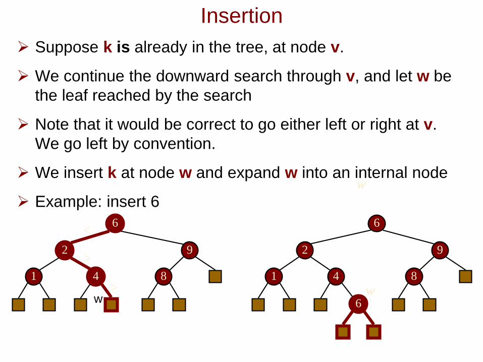
Insertion
Suppose k is already in the tree, at node v.
We continue the downward search through v, and let w be
the leaf reached by the search
Note that it would be correct to go either left or right at v.
We go left by convention.
We insert k at node w and expand w into an internal node
Example: insert 6
6
92
41 8
6
92
41 8
6
<
>
>
w
ww
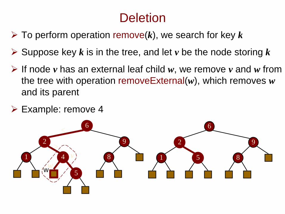
Deletion
To perform operation remove(k), we search for key k
Suppose key k is in the tree, and let v be the node storing k
If node v has an external leaf child w, we remove v and w from
the tree with operation removeExternal(w), which removes w
and its parent
Example: remove 4
6
92
41 8
5
v
w
6
92
51 8
<
>
w
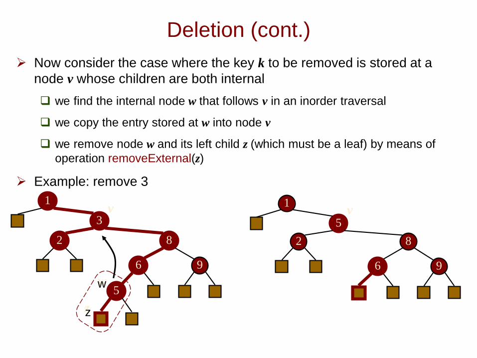
Deletion (cont.)
Now consider the case where the key k to be removed is stored at a
node v whose children are both internal
we find the internal node w that follows v in an inorder traversal
we copy the entry stored at w into node v
we remove node w and its left child z (which must be a leaf) by means of
operation removeExternal(z)
Example: remove 3
3
1
8
6 9
5
v
w
z
2
5
1
8
6 9
v
2
w
z
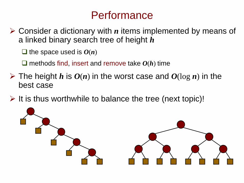
Performance
Consider a dictionary with n items implemented by means of a linked binary search tree of height h
the space used is O(n)
methods find, insert and remove take O(h) time
The height h is O(n) in the worst case and O(log n) in the best case
It is thus worthwhile to balance the tree (next topic)!
Outline
Binary Search Trees
AVL Trees
Splay Trees
AVL Trees
The AVL tree is the first balanced binary search tree
ever invented.
It is named after its two inventors, G.M. Adelson-Velskii
and E.M. Landis, who published it in their 1962 paper
"An algorithm for the organization of information.”
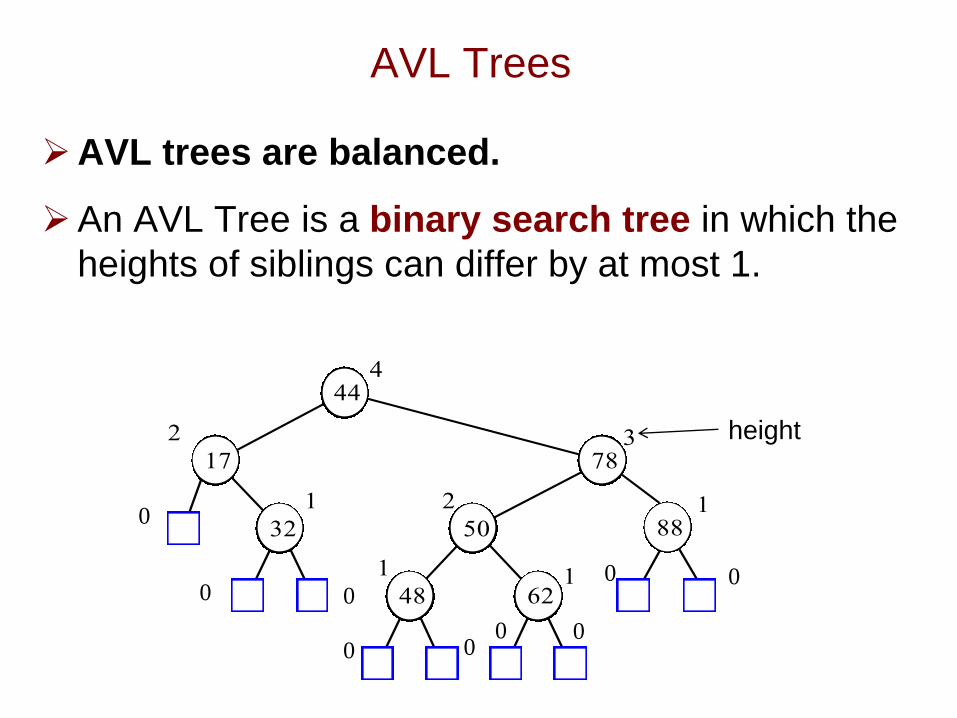
AVL Trees
AVL trees are balanced.
An AVL Tree is a binary search tree in which the
heights of siblings can differ by at most 1.
88
44
17 78
32 50
48 62
2
4
1
1
2
3
1
1
height
0
0 0
0 00 0
0 0
Height of an AVL Tree
Claim: The height of an AVL tree storing n keys is O(log n).
Height of an AVL Tree
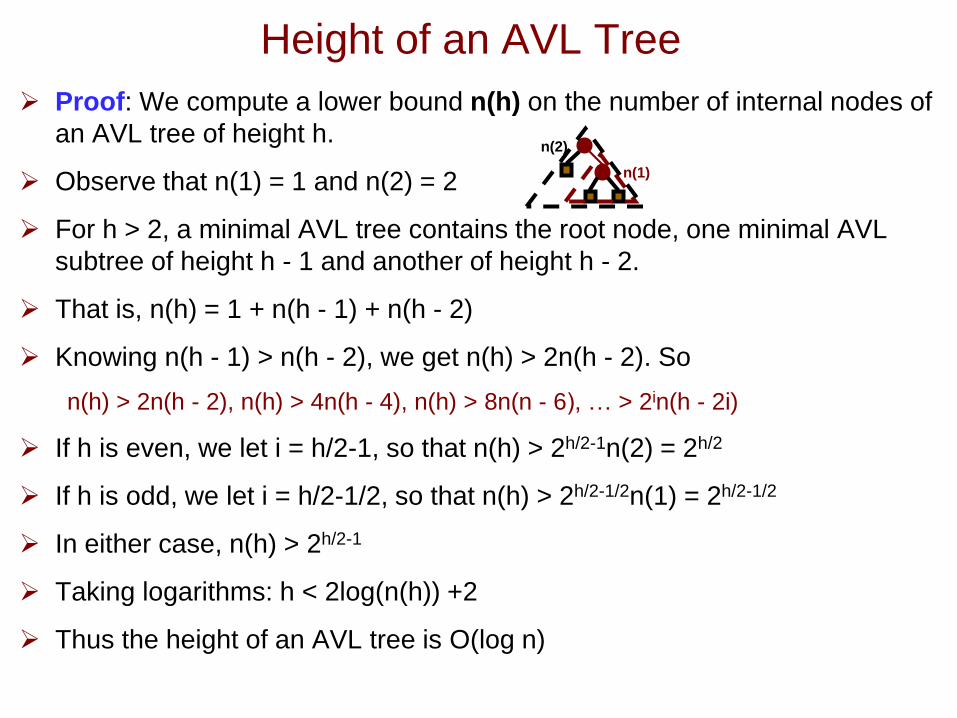
Proof: We compute a lower bound n(h) on the number of internal nodes of
an AVL tree of height h.
Observe that n(1) = 1 and n(2) = 2
For h > 2, a minimal AVL tree contains the root node, one minimal AVL
subtree of height h - 1 and another of height h - 2.
That is, n(h) = 1 + n(h - 1) + n(h - 2)
Knowing n(h - 1) > n(h - 2), we get n(h) > 2n(h - 2). So
n(h) > 2n(h - 2), n(h) > 4n(h - 4), n(h) > 8n(n - 6), … > 2in(h - 2i)
If h is even, we let i = h/2-1, so that n(h) > 2h/2-1n(2) = 2h/2
If h is odd, we let i = h/2-1/2, so that n(h) > 2h/2-1/2n(1) = 2h/2-1/2
In either case, n(h) > 2h/2-1
Taking logarithms: h < 2log(n(h)) +2
Thus the height of an AVL tree is O(log n)
3
4 n(1)
n(2)
Problem!
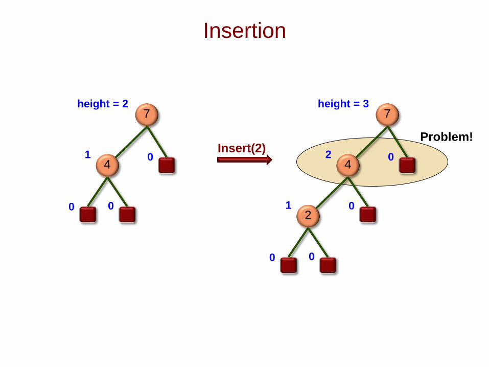
Insertion
7
4
0 0
01
height = 27
4
0
0
2
0 0
1
2
height = 3
Insert(2)
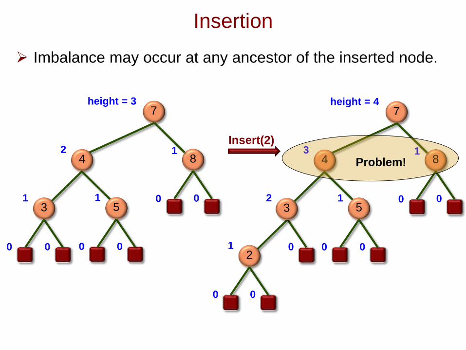
Insertion
Imbalance may occur at any ancestor of the inserted node.
Insert(2)
7
4
3
0
1
2
height = 3
8
0 0
1
0
2
2
0
10
0
5
0
1
0
7
4
3
3
height = 4
8
0 0
1
5
0
1
0
Problem!
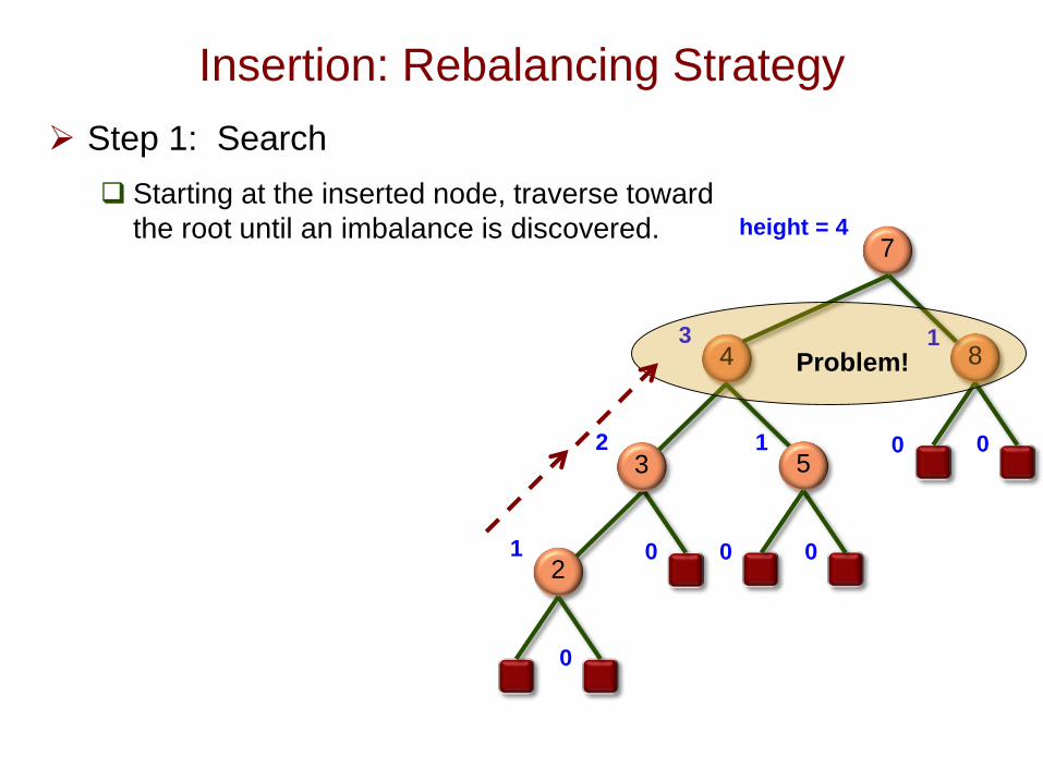
Insertion: Rebalancing Strategy
Step 1: Search
Starting at the inserted node, traverse toward
the root until an imbalance is discovered.
0
2
2
0
1
7
4
3
3
height = 4
8
0 0
1
5
0
1
0
Problem!
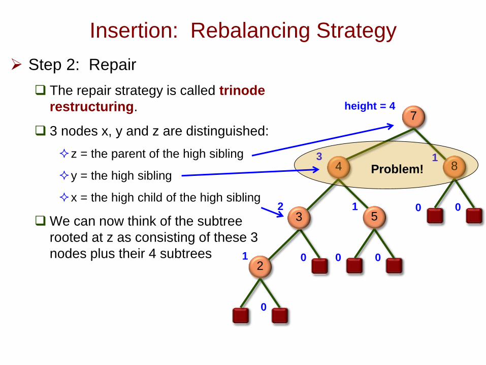
Insertion: Rebalancing Strategy
Step 2: Repair
The repair strategy is called trinode
restructuring.
3 nodes x, y and z are distinguished:
z = the parent of the high sibling
y = the high sibling
x = the high child of the high sibling
We can now think of the subtree
rooted at z as consisting of these 3
nodes plus their 4 subtrees 0
2
2
0
1
7
4
3
3
height = 4
8
0 0
1
5
0
1
0
Problem!
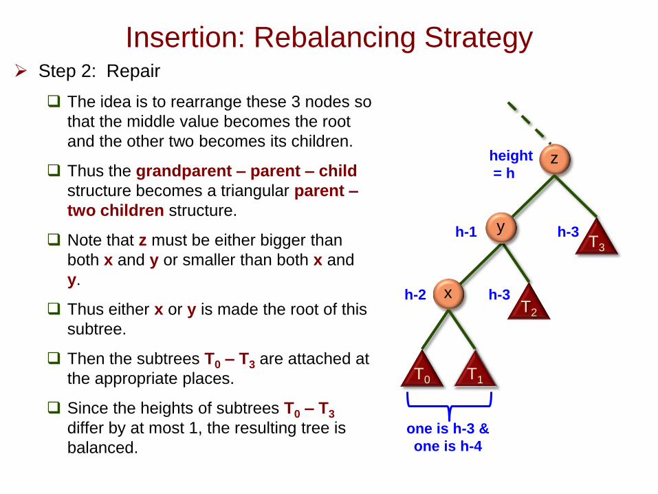
Insertion: Rebalancing Strategy Step 2: Repair
The idea is to rearrange these 3 nodes so
that the middle value becomes the root
and the other two becomes its children.
Thus the grandparent – parent – child
structure becomes a triangular parent –
two children structure.
Note that z must be either bigger than
both x and y or smaller than both x and
y.
Thus either x or y is made the root of this
subtree.
Then the subtrees T0 – T3 are attached at
the appropriate places.
Since the heights of subtrees T0 – T3
differ by at most 1, the resulting tree is
balanced.
x
z
y
height
= h
T0 T1
T2
T3
h-1 h-3
h-2
one is h-3 &
one is h-4
h-3
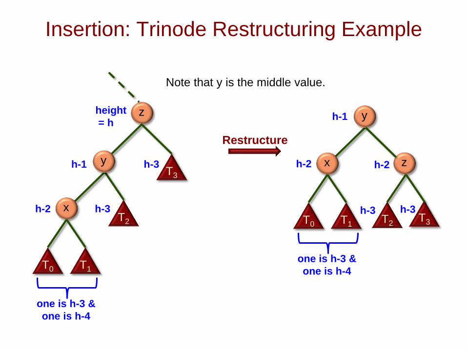
Insertion: Trinode Restructuring Example
x
z
y
height
= h
T0 T1
T2
T3
h-1 h-3
h-2
one is h-3 &
one is h-4
h-3
x z
y
T0 T1T2
T3
h-1
h-3
h-2
one is h-3 &
one is h-4
h-3
h-2
Restructure
Note that y is the middle value.
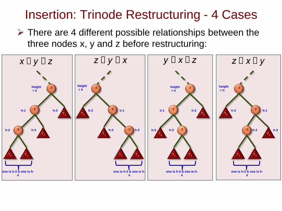
Insertion: Trinode Restructuring - 4 Cases
There are 4 different possible relationships between the
three nodes x, y and z before restructuring:
x
z
y
height
= h
T0 T1
T2
T3
h-1 h-3
h-2
one is h-3 & one is h-
4
h-3 x
z
y
height
= h
T3T2
T1
T0
h-1h-3
h-2
one is h-3 & one is h-
4
h-3 x
z
y
height
= h
T1 T2
T0
T3
h-1 h-3
h-2
one is h-3 & one is h-
4
h-3 x
z
y
height
= h
T2T1
T3
T0
h-1h-3
h-2
one is h-3 & one is h-
4
h-3
x £ y £ z z £ y £ x y £ x £ z z £ x £ y
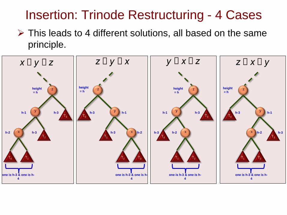
Insertion: Trinode Restructuring - 4 Cases
This leads to 4 different solutions, all based on the same
principle.
x
z
y
height
= h
T0 T1
T2
T3
h-1 h-3
h-2
one is h-3 & one is h-
4
h-3 x
z
y
height
= h
T3T2
T1
T0
h-1h-3
h-2
one is h-3 & one is h-
4
h-3 x
z
y
height
= h
T1 T2
T0
T3
h-1 h-3
h-2
one is h-3 & one is h-
4
h-3 x
z
y
height
= h
T2T1
T3
T0
h-1h-3
h-2
one is h-3 & one is h-
4
h-3
x £ y £ z z £ y £ x y £ x £ z z £ x £ y
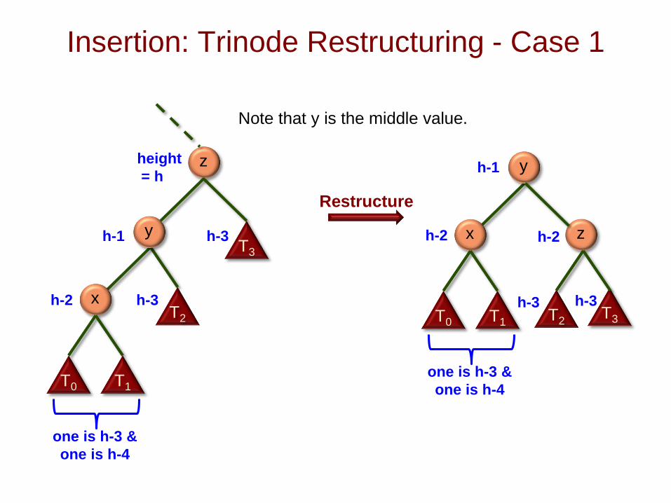
Insertion: Trinode Restructuring - Case 1
x
z
y
height
= h
T0 T1
T2
T3
h-1 h-3
h-2
one is h-3 &
one is h-4
h-3
x z
y
T0 T1T2
T3
h-1
h-3
h-2
one is h-3 &
one is h-4
h-3
h-2
Restructure
Note that y is the middle value.
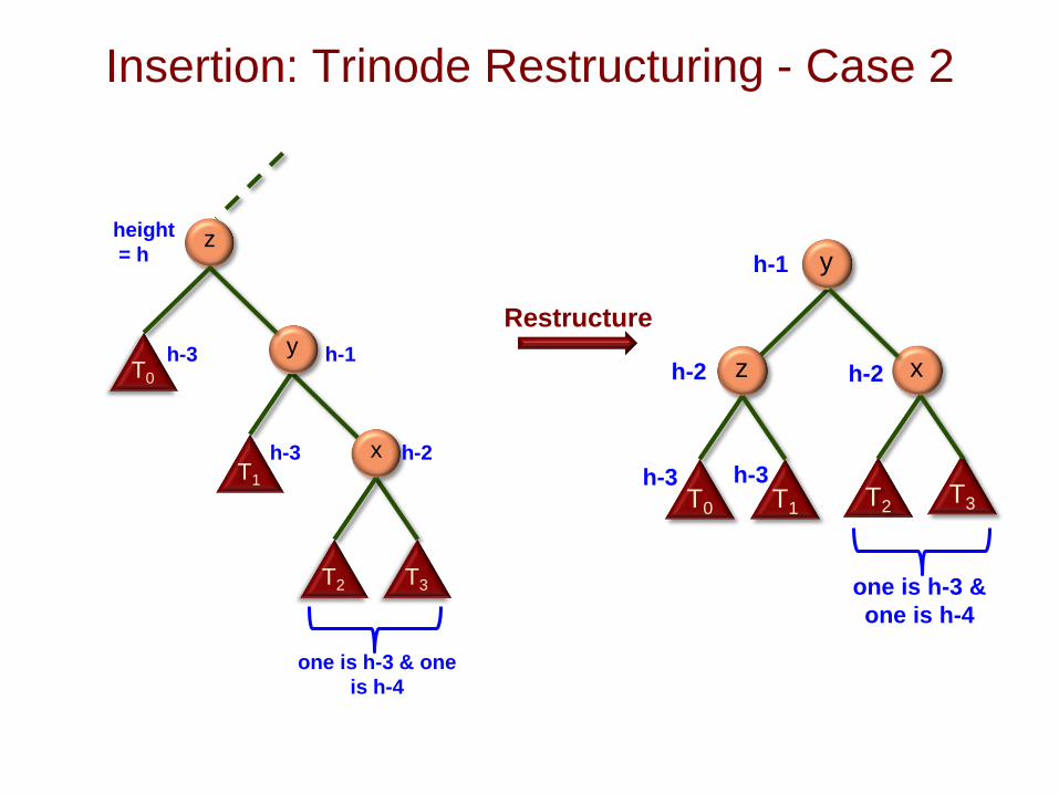
Insertion: Trinode Restructuring - Case 2
z x
y
T0 T1T2
T3
h-1
h-3
h-2
one is h-3 &
one is h-4
h-3
h-2
Restructure
x
z
y
height
= h
T3T2
T1
T0
h-1h-3
h-2
one is h-3 & one
is h-4
h-3
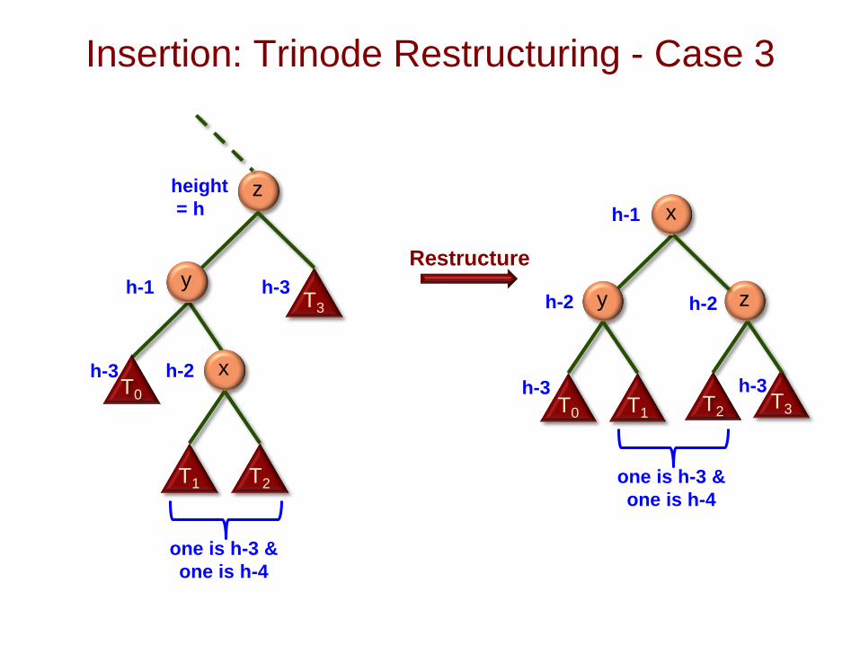
Insertion: Trinode Restructuring - Case 3
y z
x
T0 T1T2
T3
h-1
h-3
h-2
one is h-3 &
one is h-4
h-3
h-2
Restructure
x
z
y
height
= h
T1 T2
T0
T3
h-1 h-3
h-2
one is h-3 &
one is h-4
h-3
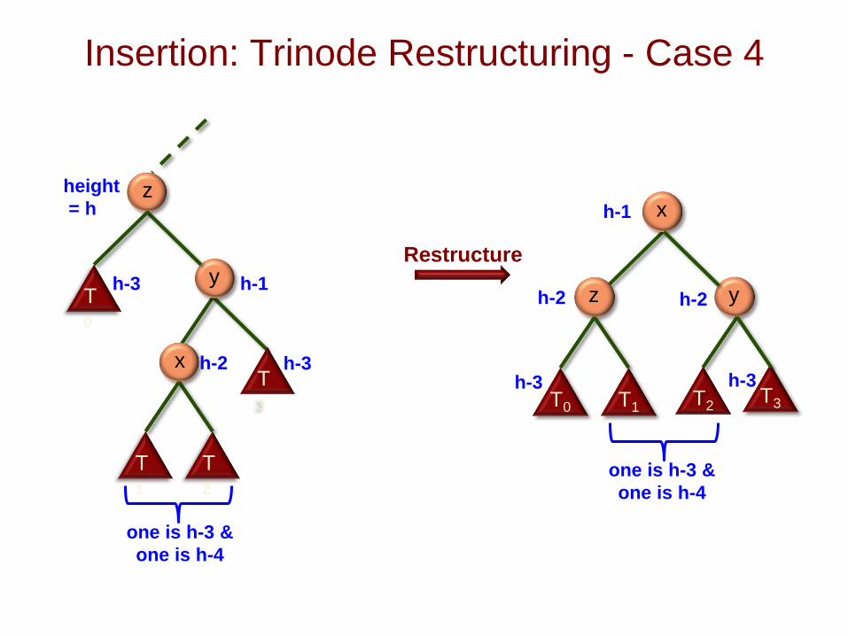
Insertion: Trinode Restructuring - Case 4
z y
x
T0 T1T2
T3
h-1
h-3
h-2
one is h-3 &
one is h-4
h-3
h-2
Restructure
x
z
y
height
= h
T2
T1
T3
T0
h-1h-3
h-2
one is h-3 &
one is h-4
h-3
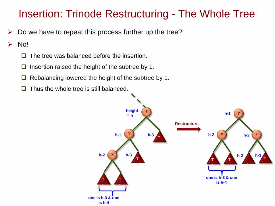
Insertion: Trinode Restructuring - The Whole Tree
Do we have to repeat this process further up the tree?
No!
The tree was balanced before the insertion.
Insertion raised the height of the subtree by 1.
Rebalancing lowered the height of the subtree by 1.
Thus the whole tree is still balanced.
x
z
y
height
= h
T0
T1
T2
T3
h-1 h-3
h-2
one is h-3 & one
is h-4
h-3
x z
y
T0
T1
T2
T3
h-1
h-3
h-2
one is h-3 & one
is h-4
h-3
h-2
Restructure
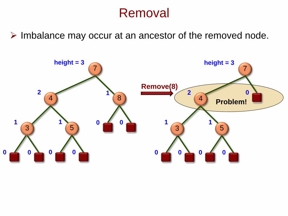
Removal
Imbalance may occur at an ancestor of the removed node.
Remove(8)
7
4
3
0
1
2
height = 3
8
0 0
1
0
1
0
5
0
1
0
7
4
3
2
height = 3
0
5
0
1
0
Problem!
0
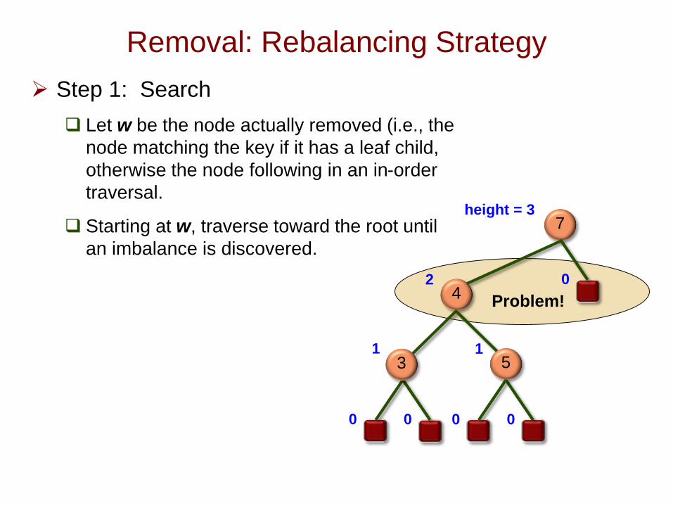
Removal: Rebalancing Strategy
Step 1: Search
Let w be the node actually removed (i.e., the
node matching the key if it has a leaf child,
otherwise the node following in an in-order
traversal.
Starting at w, traverse toward the root until
an imbalance is discovered.
0
1
0
7
4
3
2
height = 3
0
5
0
1
0
Problem!
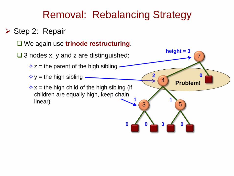
Removal: Rebalancing Strategy
Step 2: Repair
We again use trinode restructuring.
3 nodes x, y and z are distinguished:
z = the parent of the high sibling
y = the high sibling
x = the high child of the high sibling (if
children are equally high, keep chain
linear)
0
1
0
7
4
3
2
height = 3
0
5
0
1
0
Problem!

Removal: Rebalancing Strategy
Step 2: Repair
The idea is to rearrange these 3 nodes so
that the middle value becomes the root
and the other two becomes its children.
Thus the grandparent – parent – child
structure becomes a triangular parent –
two children structure.
Note that z must be either bigger than
both x and y or smaller than both x and
y.
Thus either x or y is made the root of this
subtree, and z is lowered by 1.
Then the subtrees T0 – T3 are attached at
the appropriate places.
Although the subtrees T0 – T3 can differ in
height by up to 2, after restructuring,
sibling subtrees will differ by at most 1.
x
z
y
height
= h
T0 T1
T2
T3
h-1 h-3
h-2
h-3 or h-3 & h-
4
h-2
or
h-3
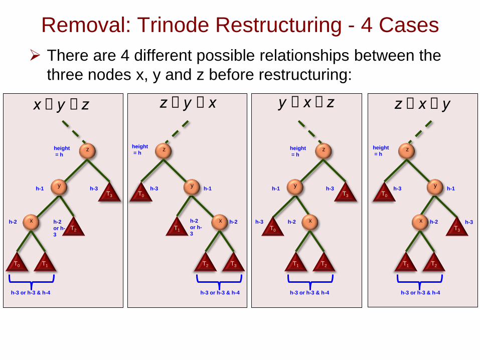
Removal: Trinode Restructuring - 4 Cases
There are 4 different possible relationships between the
three nodes x, y and z before restructuring:
x
z
y
height
= h
T0 T1
T2
T3
h-1 h-3
h-2
h-3 or h-3 & h-4
h-2
or h-
3
x
z
y
height
= h
T3T2
T1
T0
h-1h-3
h-2
h-3 or h-3 & h-4
h-2
or h-
3
x
z
y
height
= h
T1 T2
T0
T3
h-1 h-3
h-2
h-3 or h-3 & h-4
h-3 x
z
y
height
= h
T2T1
T3
T0
h-1h-3
h-2
h-3 or h-3 & h-4
h-3
x £ y £ z z £ y £ x y £ x £ z z £ x £ y
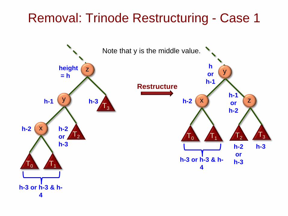
Removal: Trinode Restructuring - Case 1
x
z
y
height
= h
T0 T1
T2
T3
h-1 h-3
h-2
h-3 or h-3 & h-
4
h-2
or
h-3
x z
y
T0 T1T2
T3
h
or
h-1
h-3
h-2
h-3 or h-3 & h-
4
h-2
or
h-3
h-1
or
h-2
Restructure
Note that y is the middle value.
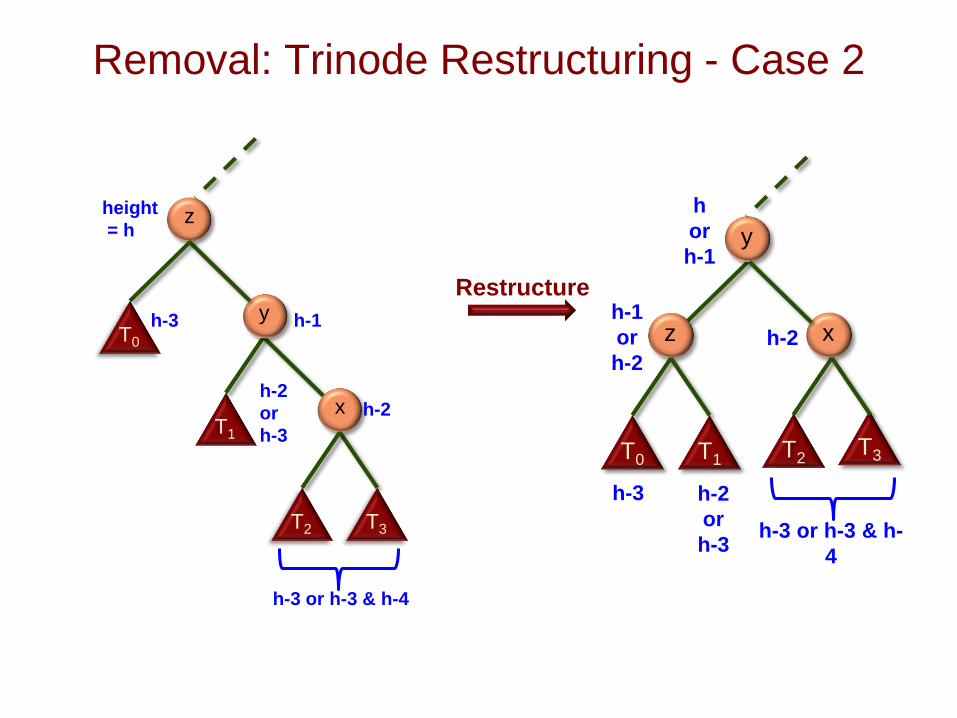
Removal: Trinode Restructuring - Case 2
z x
y
T0 T1T2
T3
h
or
h-1
h-2
or
h-3
h-1
or
h-2
h-3 or h-3 & h-
4
h-3
h-2
Restructure
x
z
y
height
= h
T3T2
T1
T0
h-1h-3
h-2
h-3 or h-3 & h-4
h-2
or
h-3
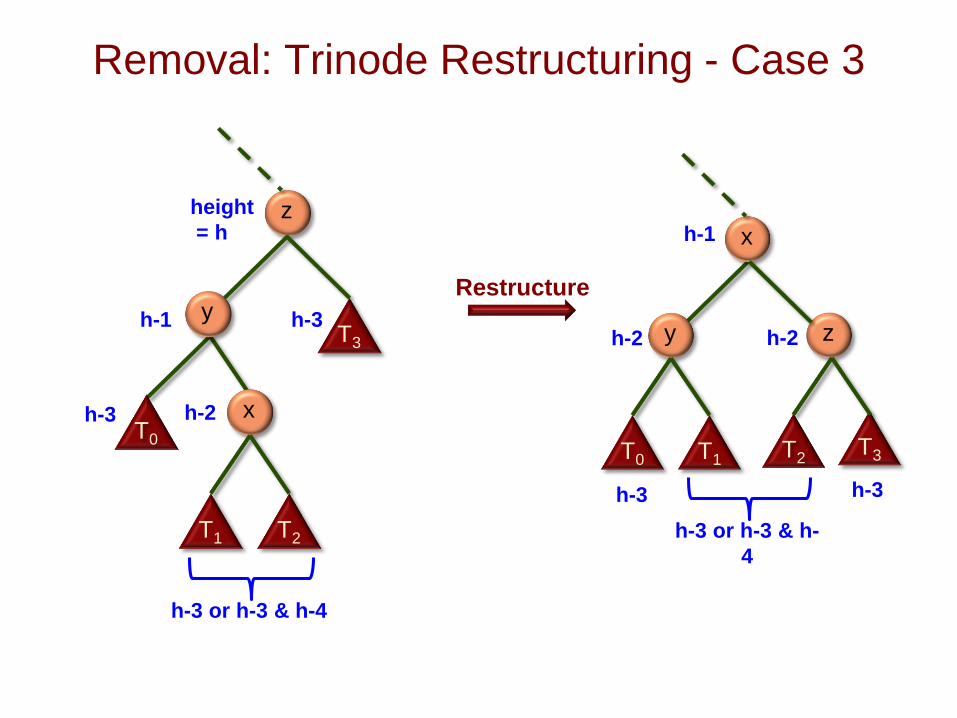
Removal: Trinode Restructuring - Case 3
y z
x
T0 T1T2
T3
h-1
h-3
h-2
h-3 or h-3 & h-
4
h-3
h-2
Restructure
x
z
y
height
= h
T1 T2
T0
T3
h-1 h-3
h-2
h-3 or h-3 & h-4
h-3
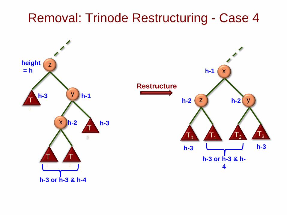
Removal: Trinode Restructuring - Case 4
z y
x
T0 T1T2
T3
h-1
h-3
h-2
h-3 or h-3 & h-
4
h-3
h-2
Restructure
x
z
y
height
= h
T2
T1
T3
T0
h-1h-3
h-2
h-3 or h-3 & h-4
h-3
Removal: Rebalancing Strategy
Step 2: Repair
Unfortunately, trinode restructuring may
reduce the height of the subtree, causing
another imbalance further up the tree.
Thus this search and repair process must
in the worst case be repeated until we
reach the root.

Java Implementation of AVL Trees
Please see text
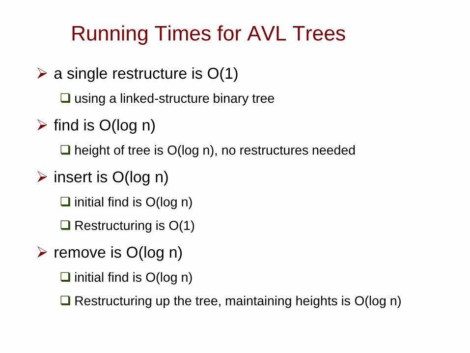
Running Times for AVL Trees
a single restructure is O(1)
using a linked-structure binary tree
find is O(log n)
height of tree is O(log n), no restructures needed
insert is O(log n)
initial find is O(log n)
Restructuring is O(1)
remove is O(log n)
initial find is O(log n)
Restructuring up the tree, maintaining heights is O(log n)
AVLTree Example
Outline
Binary Search Trees
AVL Trees
Splay Trees
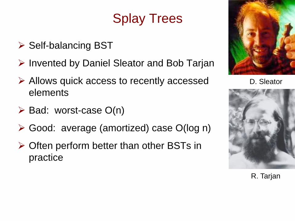
Splay Trees
Self-balancing BST
Invented by Daniel Sleator and Bob Tarjan
Allows quick access to recently accessed
elements
Bad: worst-case O(n)
Good: average (amortized) case O(log n)
Often perform better than other BSTs in
practice
D. Sleator
R. Tarjan
Splaying
Splaying is an operation performed on a node that
iteratively moves the node to the root of the tree.
In splay trees, each BST operation (find, insert, remove)
is augmented with a splay operation.
In this way, recently searched and inserted elements are
near the top of the tree, for quick access.
3 Types of Splay Steps
Each splay operation on a node consists of a sequence
of splay steps.
Each splay step moves the node up toward the root by 1
or 2 levels.
There are 2 types of step:
Zig-Zig
Zig-Zag
Zig
These steps are iterated until the node is moved to the
root.
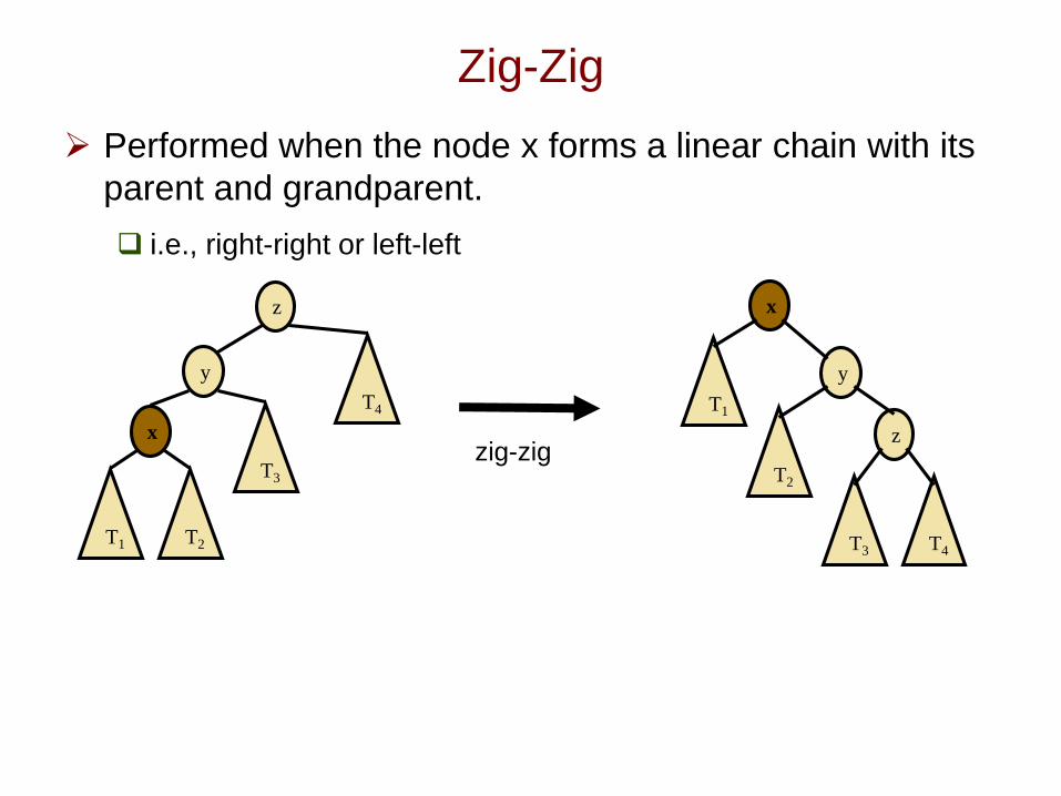
Zig-Zig
Performed when the node x forms a linear chain with its
parent and grandparent.
i.e., right-right or left-left
y
x
T1 T2
T3
z
T4
zig-zig
y
z
T4T3
T2
x
T1
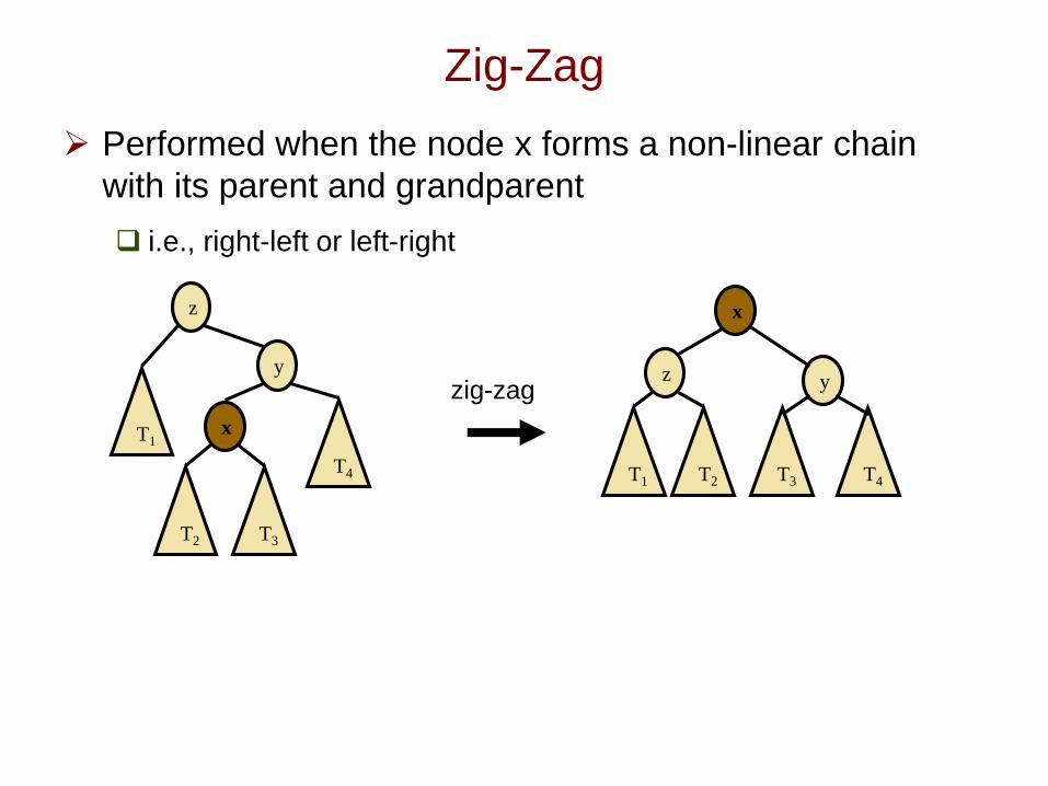
Zig-Zag
Performed when the node x forms a non-linear chain
with its parent and grandparent
i.e., right-left or left-right
zig-zagy
x
T2 T3
T4
z
T1
y
x
T2 T3 T4
z
T1
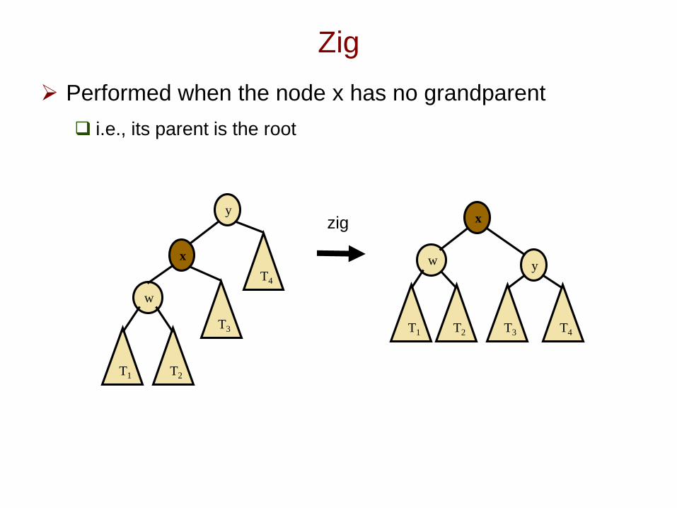
Zig
Performed when the node x has no grandparent
i.e., its parent is the root
zig
x
w
T1 T2
T3
y
T4
y
x
T2 T3 T4
w
T1
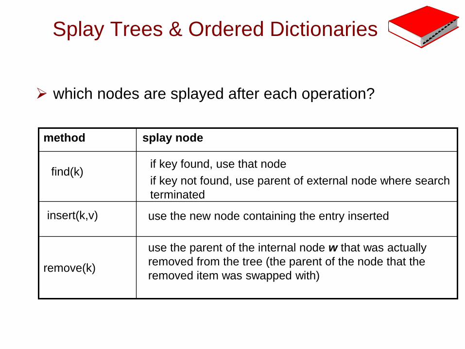
Splay Trees & Ordered Dictionaries
which nodes are splayed after each operation?
use the parent of the internal node w that was actually
removed from the tree (the parent of the node that the
removed item was swapped with)remove(k)
use the new node containing the entry insertedinsert(k,v)
if key found, use that node
if key not found, use parent of external node where search
terminated
find(k)
splay nodemethod
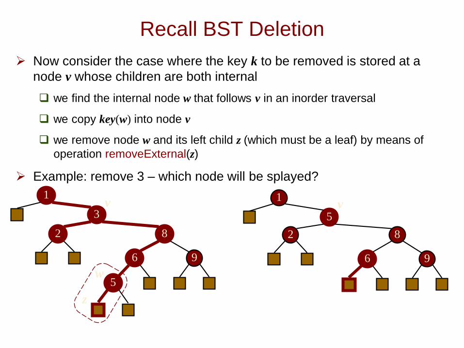
Recall BST Deletion
Now consider the case where the key k to be removed is stored at a
node v whose children are both internal
we find the internal node w that follows v in an inorder traversal
we copy key(w) into node v
we remove node w and its left child z (which must be a leaf) by means of
operation removeExternal(z)
Example: remove 3 – which node will be splayed?
3
1
8
6 9
5
v
w
z
2
5
1
8
6 9
v
2
Note on Deletion
The text (Goodrich, p. 463) uses a different convention
for BST deletion in their splaying example
Instead of deleting the leftmost internal node of the right subtree,
they delete the rightmost internal node of the left subtree.
We will stick with the convention of deleting the leftmost internal
node of the right subtree (the node immediately following the
element to be removed in an inorder traversal).
Splay Tree Example
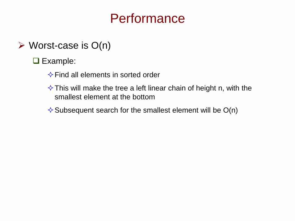
Performance
Worst-case is O(n)
Example:
Find all elements in sorted order
This will make the tree a left linear chain of height n, with the
smallest element at the bottom
Subsequent search for the smallest element will be O(n)
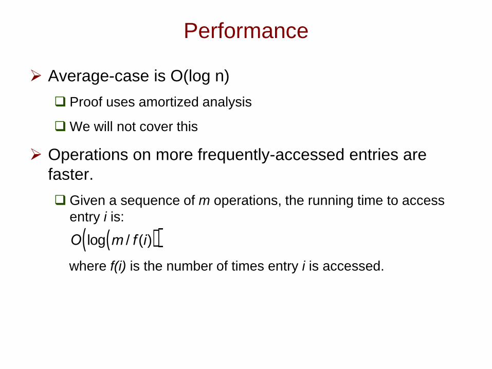
Performance
Average-case is O(log n)
Proof uses amortized analysis
We will not cover this
Operations on more frequently-accessed entries are
faster.
Given a sequence of m operations, the running time to access
entry i is:
where f(i) is the number of times entry i is accessed. O log m / f (i)( )( )
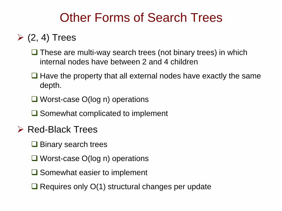
Other Forms of Search Trees
(2, 4) Trees
These are multi-way search trees (not binary trees) in which
internal nodes have between 2 and 4 children
Have the property that all external nodes have exactly the same
depth.
Worst-case O(log n) operations
Somewhat complicated to implement
Red-Black Trees
Binary search trees
Worst-case O(log n) operations
Somewhat easier to implement
Requires only O(1) structural changes per update
Summary
Binary Search Trees
AVL Trees
Splay Trees


