BiNoM 2.0, a Cytoscape plugin for accessing and

analyzing pathways using standard systems biology

formats.

Eric Bonnet, Laurence Calzone, Daniel Rovera, Gautier Stoll, Emmanuel

Barillot, Andrei Zinovyev

To cite this version:

Eric Bonnet, Laurence Calzone, Daniel Rovera, Gautier Stoll, Emmanuel Barillot, et al.. Bi-NoM 2.0, a Cytoscape plugin for accessing and analyzing pathways using standard systemsbiology formats.. BMC Systems Biology, BioMed Central, 2013, 7 (1), pp.18. <10.1186/1752-0509-7-18>. <inserm-00820930>

HAL Id: inserm-00820930

http://www.hal.inserm.fr/inserm-00820930

Submitted on 7 May 2013

HAL is a multi-disciplinary open accessarchive for the deposit and dissemination of sci-entific research documents, whether they are pub-lished or not. The documents may come fromteaching and research institutions in France orabroad, or from public or private research centers.

L’archive ouverte pluridisciplinaire HAL, estdestinee au depot et a la diffusion de documentsscientifiques de niveau recherche, publies ou non,emanant des etablissements d’enseignement et derecherche francais ou etrangers, des laboratoirespublics ou prives.

Bonnet et al. BMC Systems Biology 2013, 7:18

http://www.biomedcentral.com/1752-0509/7/18

SOFTWARE Open Access

BiNoM 2.0, a Cytoscape plugin for accessingand analyzing pathways using standardsystems biology formatsEric Bonnet1,2,3, Laurence Calzone1,2,3, Daniel Rovera1,2,3, Gautier Stoll1,2,3, Emmanuel Barillot1,2,3,

and Andrei Zinovyev1,2,3*

Abstract

Background: Public repositories of biological pathways and networks have greatly expanded in recent years. Such

databases contain many pathways that facilitate the analysis of high-throughput experimental work and the

formulation of new biological hypotheses to be tested, a fundamental principle of the systems biology approach.

However, large-scale molecular maps are not always easy to mine and interpret.

Results: We have developed BiNoM (Biological Network Manager), a Cytoscape plugin, which provides functions for

the import-export of some standard systems biology file formats (import from CellDesigner, BioPAX Level 3 and CSML;

export to SBML, CellDesigner and BioPAX Level 3), and a set of algorithms to analyze and reduce the complexity of

biological networks. BiNoM can be used to import and analyze files created with the CellDesigner software. BiNoM

provides a set of functions allowing to import BioPAX files, but also to search and edit their content. As such, BiNoM is

able to efficiently manage large BioPAX files such as whole pathway databases (e.g. Reactome). BiNoM also implements

a collection of powerful graph-based functions and algorithms such as path analysis, decomposition by involvement

of an entity or cyclic decomposition, subnetworks clustering and decomposition of a large network in modules.

Conclusions: Here, we provide an in-depth overview of the BiNoM functions, and we also detail novel aspects such

as the support of the BioPAX Level 3 format and the implementation of a new algorithm for the quantification of

pathways for influence networks. At last, we illustrate some of the BiNoM functions on a detailed biological case study

of a network representing the G1/S transition of the cell cycle, a crucial cellular process disturbed in most human

tumors.

Keywords: Systems biology, Cytoscape, Software, SBML, BioPAX, CellDesigner, Conversion, SBGN, Reactome,

Network analysis, Path analysis, Molecular maps, Pathways

BackgroundBiological pathways and networks comprise sets of inter-

actions, or functional relationships, occurring at the

molecular level in living cells [1,2]. A large body of

knowledge on cellular biochemistry is organized in pub-

licly available repositories such as the KEGG database

[3], Reactome [4], MINT [5], or the Cancer Cell Map

(http://cancer.cellmap.org/) . All these pathway and bio-

logical network databases facilitate a large spectrum of

*Correspondence: andrei.zinovyev@curie.fr1Institut Curie, 26 rue d’Ulm, Paris, F-75248 France2INSERM, U900, Paris, F-75248 France

Full list of author information is available at the end of the article

analyses, improving our understanding of cellular sys-

tems. For example, it is now a very common practice to

cross the output of high-throughput experiments, such as

mRNA or protein expression levels, with curated biolog-

ical pathways in order to visualize changes, analyze their

impact on a network and formulate new hypotheses about

biological processes [6,7]. The development of those path-

way repositories has also fueled the creation of standard

representations and formats, to facilitate the exchange

and representation of data, such as the Biological Path-

way Exchange standard (BioPAX) [8], the Systems Biology

Markup Language (SBML) [9] or the Systems Biology

Graphical Notation (SBGN) [10]. The Pathguide website

© 2013 Bonnet et al.; licensee BioMed Central Ltd. This is an Open Access article distributed under the terms of the CreativeCommons Attribution License (http://creativecommons.org/licenses/by/2.0), which permits unrestricted use, distribution, andreproduction in any medium, provided the original work is properly cited.

Bonnet et al. BMC Systems Biology 2013, 7:18 Page 2 of 16

http://www.biomedcentral.com/1752-0509/7/18

counts more than 300 web-accessible biological pathway

and network databases [11], many of which are using the

SBML and BioPAX standard formats. Ultimately, those

integrated resources will facilitate computational model

building, their exchange, re-usability and their experimen-

tal validation, a cycle that is the cornerstone of the systems

biology approach [12-14].

As a consequence, there is a need for the precise and

accurate construction of pathways and large-scale molec-

ular maps covering fundamental biological processes.

Such maps are often constructed by manual curation

of the literature or automated curation from pathway

databases [15]. More and more, they are focused on the

regulation of biological processes involved in diseases

such as cancer, Alzheimer’s disease or Crohn’s disease, to

name a few [16-19]. However, the scale of suchmaps, even

when they are focusing on a particular process, is quite

large, with hundreds of chemical species and interactions.

The analysis and interpretation of such maps is therefore

not a straightforward task. Several computational tools

have been developed to facilitate the visualization, cura-

tion and analysis of pathways [1]. For example, CellDe-

signer is a software package for the graphical editing of

biological pathway diagrams [20]. CellDesigner files are

using the SBML format specification, with specific exten-

sions describing biological types of chemical species and

the layout of the reaction graph. There is obviously a

need for user-friendly software tools that would allow the

user to easily import data from various standard format

sources, to perform structural analyses on these pathways

and to manipulate networks, and to be able to export

a network to a suitable format for further analysis. We

have created BiNoM [21], a software plugin for the popu-

lar Cytoscape network vizualization and analysis tool [22]

precisely to fulfill this purpose. There are several tools

available for the import, visualisation and export of stan-

dard systems biology file formats, as well as their their

conversion [20,23-26]. There is also a significant number

of tools for network analysis [27-31]. However, we think

that the strength of BiNoM is to provide at the same time

a strong support for a choice of systems biology file for-

mats, a set of robust and powerful network analysis tools,

and also some very speficic functions that are not avail-

able in any other tool at the moment (see Table 1 for

a detailed comparison of BiNoM’s function with other

tools). BiNoM is designed to be useful in a finite set of

pragmatic, user-oriented and proved to be needed scenar-

ios for biological networks analysis. For instance, a user

may want to import a molecular map from a CellDe-

signer file, analyze it using graph-based algorithms, and

finally export a subnetwork of interest to the SBML format

for mathematical modeling using a dedicated software.

Obviously, it is rather complicated to provide robust sup-

port for all the standard systems biology formats that are

now available. We have therefore implemented functions

in BiNoM for importing and exporting from and to a

selection of file formats (CellDesigner, BioPAX Level 3,

CSML, SBML, see Table 2 for a detailed information on

the exact import/export possibilities of BiNoM). BiNoM

uses its own ontology for the graphical representation of

the different entities and their relationships. The graphi-

cal conventions in BiNoM are inspired by the ones defined

for the SBGN standard (see the BiNoM manual chapter 8

for amore complete description). BiNoM also implements

several functions based on graph operations for the struc-

tural analysis of biological networks. Those functions can

be used to reduce the complexity and extract meaning-

ful subnetworks from large-scale molecular maps. Here,

we provide a detailed view on the functions imple-

mented in BiNoM that permit specific extraction of

information frommolecularmaps and improve their read-

ability and usability. We also highlight novel functions

that were implemented recently, such as the support of

the latest BioPAX specification (BioPAX Level 3) and

an algorithmic approach for the quantification of path-

ways on influence networks (PIQuant, Pathway Influence

Quantification algorithm). We illustrate the use of the

principal BiNoM functions with a detailed analysis of

a molecular network of the G1/S transition of the cell

cycle, a central mechanism for tumor development and

progression.

ImplementationBiNoM is implemented in the JavaTM programming lan-

guage, as a plugin for the network visualization and

analysis software package Cytoscape [22]. Although the

primary use of BiNoM is through the Cytoscape software,

the underlying logic of most of the BiNoM functions is

completely decoupled from the Cytoscape objects, allow-

ing developers to also use BiNoM as an independent

Java library [21]. The installation of BiNoM can be done

through the Cytoscape plugin manager (menu “Plugins >

Manage Plugins”, Section “Other”, then select the latest

version of BiNoM). Alternatively, the user can also down-

load the plugin together with a manual and the source

code from the BiNoM website (http://binom.curie.fr/).

BiNoM manipulates the information contained in stan-

dard systems biology files by mapping it onto a labeled

graph, called index. The index does not try to map the

totality of all details but rather serves as a connection map

for the objects contained in other ontologies. The index

contains the minimum information needed to graphically

represent objects and connections between them. BiNoM

index is a light-weight construction which can be easily

regenerated, does not duplicate the information in exist-

ing files and serves only to facilitate the visualization and

to access existing systems biology files. Currently, BiNoM

index is mostly developed to map BioPAX ontology files

Bonnetetal.BMCSystem

sBiology2013,7:18

Page3of16

http

://www.biomedcentra

l.com/1752-0509/7/18

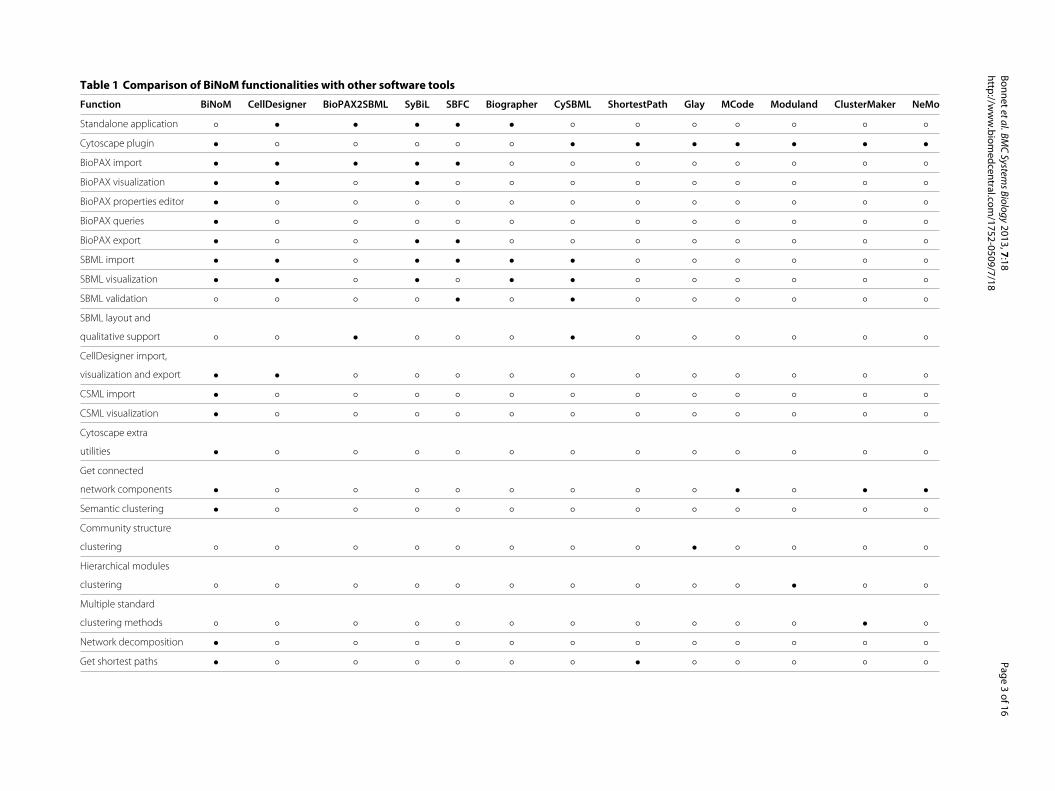
Table 1 Comparison of BiNoM functionalities with other software tools

Function BiNoM CellDesigner BioPAX2SBML SyBiL SBFC Biographer CySBML ShortestPath Glay MCode Moduland ClusterMaker NeMo

Standalone application ◦ • • • • • ◦ ◦ ◦ ◦ ◦ ◦ ◦

Cytoscape plugin • ◦ ◦ ◦ ◦ ◦ • • • • • • •

BioPAX import • • • • • ◦ ◦ ◦ ◦ ◦ ◦ ◦ ◦

BioPAX visualization • • ◦ • ◦ ◦ ◦ ◦ ◦ ◦ ◦ ◦ ◦

BioPAX properties editor • ◦ ◦ ◦ ◦ ◦ ◦ ◦ ◦ ◦ ◦ ◦ ◦

BioPAX queries • ◦ ◦ ◦ ◦ ◦ ◦ ◦ ◦ ◦ ◦ ◦ ◦

BioPAX export • ◦ ◦ • • ◦ ◦ ◦ ◦ ◦ ◦ ◦ ◦

SBML import • • ◦ • • • • ◦ ◦ ◦ ◦ ◦ ◦

SBML visualization • • ◦ • ◦ • • ◦ ◦ ◦ ◦ ◦ ◦

SBML validation ◦ ◦ ◦ ◦ • ◦ • ◦ ◦ ◦ ◦ ◦ ◦

SBML layout and

qualitative support ◦ ◦ • ◦ ◦ ◦ • ◦ ◦ ◦ ◦ ◦ ◦

CellDesigner import,

visualization and export • • ◦ ◦ ◦ ◦ ◦ ◦ ◦ ◦ ◦ ◦ ◦

CSML import • ◦ ◦ ◦ ◦ ◦ ◦ ◦ ◦ ◦ ◦ ◦ ◦

CSML visualization • ◦ ◦ ◦ ◦ ◦ ◦ ◦ ◦ ◦ ◦ ◦ ◦

Cytoscape extra

utilities • ◦ ◦ ◦ ◦ ◦ ◦ ◦ ◦ ◦ ◦ ◦ ◦

Get connected

network components • ◦ ◦ ◦ ◦ ◦ ◦ ◦ ◦ • ◦ • •

Semantic clustering • ◦ ◦ ◦ ◦ ◦ ◦ ◦ ◦ ◦ ◦ ◦ ◦

Community structure

clustering ◦ ◦ ◦ ◦ ◦ ◦ ◦ ◦ • ◦ ◦ ◦ ◦

Hierarchical modules

clustering ◦ ◦ ◦ ◦ ◦ ◦ ◦ ◦ ◦ ◦ • ◦ ◦

Multiple standard

clustering methods ◦ ◦ ◦ ◦ ◦ ◦ ◦ ◦ ◦ ◦ ◦ • ◦

Network decomposition • ◦ ◦ ◦ ◦ ◦ ◦ ◦ ◦ ◦ ◦ ◦ ◦

Get shortest paths • ◦ ◦ ◦ ◦ ◦ ◦ • ◦ ◦ ◦ ◦ ◦

Bonnetetal.BMCSystem

sBiology2013,7:18

Page4of16

http

://www.biomedcentra

l.com/1752-0509/7/18

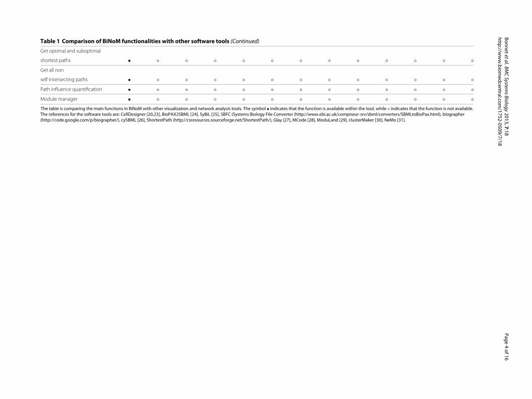
Table 1 Comparison of BiNoM functionalities with other software tools (Continued)

Get optimal and suboptimal

shortest paths • ◦ ◦ ◦ ◦ ◦ ◦ ◦ ◦ ◦ ◦ ◦ ◦

Get all non

self-intersecting paths • ◦ ◦ ◦ ◦ ◦ ◦ ◦ ◦ ◦ ◦ ◦ ◦

Path influence quantification • ◦ ◦ ◦ ◦ ◦ ◦ ◦ ◦ ◦ ◦ ◦ ◦

Module manager • ◦ ◦ ◦ ◦ ◦ ◦ ◦ ◦ ◦ ◦ ◦ ◦

The table is comparing the main functions in BiNoM with other visualization and network analysis tools. The symbol • indicates that the function is available within the tool, while ◦ indicates that the function is not available.

The references for the software tools are: CellDesigner [20,23], BioPAX2SBML [24], SyBiL [25], SBFC (Systems Biology File Converter (http://www.ebi.ac.uk/compneur-srv/sbml/converters/SBMLtoBioPax.html), biographer

(http://code.google.com/p/biographer/), cySBML [26], ShortestPath (http://csresources.sourceforge.net/ShortestPath/), Glay [27], MCode [28], ModuLand [29], clusterMaker [30], NeMo [31].

Bonnet et al. BMC Systems Biology 2013, 7:18 Page 5 of 16

http://www.biomedcentral.com/1752-0509/7/18

Table 2 Detailed import/export BiNoM capabilities for

standard systems biology file formats

Import from Export (from / to)

CellDesigner v3.x, 4.1, 4.2 BioPAX Level 3 / BioPAX Level 3

BioPAX Level 3 BioPAX Level 3 / SBML Level 2

SBML Level 2 CellDesigner v3.x, 4.1, 4.2 / CellDesigner v4.1

CSML v3.0 CellDesigner v3.x, 4.1, 4.2 / BioPAX Level 3

CellDesigner v3.x, 4.1, 4.2 / SBML Level 2

CSML v3.0 / SBML Level 2

The table is indicating the different standard systems biology file formats and

versions that can be currently imported/exported in BiNoM, as well as what type

of conversions are possible.

and CellDesigner object schema. More specifically, we use

XmlBeans (http://xmlbeans.apache.org/) to create Java

classes from the xml definition file in order to access all the

elements contained in the CellDesigner, SBML and CSML

files. BioPAX uses the web ontology language specifi-

cation (OWL, (http://www.w3.org/2004/OWL/) to store

data in XML-formatted files. In BiNoM, we use the Jas-

tor and the Jena Java libraries (http://jastor.sourceforge.

net/), (http://jena.sourceforge.net/) to automatically cre-

ate Java classes from the BioPAX specifications, allowing

a convenient access to the different data types encoded in

the BioPAX files. More detailed informations about the

index and the mapping are available in the BiNoMmanual

(http://binom.curie.fr).

The core functions of BiNoM can be grouped in five dif-

ferent topics: Input/Output, Structural Analysis, BioPAX

utils & query, Module manager and Utilities.

BiNoM input / output

BiNoM functions facilitate the import and export of some

of the standard systems biology file formats, but BiNoM

plugin is not designed to be a universal converter (for a

complete list of the different import/export possibilities in

BiNoM, see Table 2). For instance, BiNoMwill be useful in

the examples of conversion and analysis scenarios detailed

below (non-exhaustive list):

• Interconversion of CellDesigner files to BioPAX, and

from a BioPAX reaction network to SBML Level 2.• Import of a BioPAX file as a reaction network and/or

a pathway structure and/or an interaction map,

followed by the creation of a subnetwork saved as a

new BioPAX file.• Import of a BioPAX file, selection of a subnetwork of

interest saved as a SBML file for the creation of a

computational model using an appropriate software

package, such as CellDesigner [20] or GINsim [32].• Import a large CellDesigner map and export only a

subnetwork as a new CellDesigner file.

The BioPAX community has recently made a major

update of the BioPAX standard, producing a new spec-

ification known as BioPAX Level 3 (http://www.biopax.

org/). This format supports metabolic pathways, sig-

naling pathways (including states of molecules and

generic molecules), gene regulatory networks, molec-

ular interactions and genetic interactions. Due to

major changes in the specification, the BioPAX Level

3 is not backward compatible with the Level 2 file

format.

BioPAX Level 3 files are imported as three separate

graphs, respectively the Reaction Network (RN), repre-

senting the biochemical reaction network, the Pathway

Structure (PS), showing the hierarchical organisation of

pathways, and the Interaction Map graph (IM). At the

moment, the MIRIAM annotations are not imported in

BiNoM, but we plan to provide access to this type infor-

mation soon. Several examples of simple BioPAX Level

3 files imported through BiNoM, representing different

types of interactions, are shown on Figure 1. Figure 2

shows the hierarchical structure of the human apoptosis

pathway, extracted from Reactome database, and con-

structed by BiNoM.

When importing a file, BiNoM is calling a naming ser-

vice function in order to create meaningful names for the

various entities. More precisely, entity names are com-

bined with other features such as modifications, compart-

ment and complex components. The different features

are indicated by special characters, such as “@” for the

compartments, “|” for modifications and “:” to delimi-

tate the different members of a complex. For example,

the name Cdc25|Pho@cytoplasm represents the protein

Cdc25 in a phosphorylated state, located in the cytoplasm,

while the name Cdc13:Cdc2|Thr167 pho@cytoplasm

indicates a protein complex located in the cytosplasm,

composed of the protein Cdc13 and the protein

Cdc2 phosphorylated at position 167 on a threonine

residue.

BiNoM structural analysis

The central goal of the BiNoM plugin is to provide effi-

cient methods and algorithms to reduce the inherent

complexity of biological networks into manageable and

meaningful subnetworks. This goal is achieved by a set

of functions included as a built-in structural graph anal-

ysis library. Some of the functions take into account

the semantics contained in the graph element names.

The structural analysis functions implemented in BiNoM

include the identification of connected and strongly con-

nected components, pruning of the network, decomposi-

tion by involvement of a protein (material components)

or by cyclic decomposition, path analysis and network

clustering. We also introduce in this version of BiNoM

a novel function to quantify the influence of a source

Bonnet et al. BMC Systems Biology 2013, 7:18 Page 6 of 16

http://www.biomedcentral.com/1752-0509/7/18

Figure 1 Visualization of the six BioPAX example files, provided in BioPAX 3.0 documentation. The BioPAX 3.0 documentation available at

http://biopax.org contains six simple examples of BioPAX 3.0 files that describe different aspects of biological network interactions (genetic

interaction, short metabolic pathway, gene regulatory network, biochemical reaction, phosphorylation, protein interaction). Here we show how

BiNoM visualizes these examples after their import. The BiNoM type of representation is indicated below the reaction type, in brackets (Reaction

Network, Pathway Structure and Interaction Map). The graphical node and edge semantic is described in more details in the BiNoMmanual.

node on a target node taking into account experimen-

tal data, called PIQuant. In the following paragraphs,

we will detail network decomposition and the PIQuant

score.

Decomposition by involvement of a protein or by cyclic

decomposition

BiNoM proposes three methods to dissect a complex bio-

logical network into parts. A trivial approach to separate

a network into subparts is to dissociate the unconnected

subparts of the network. A more sophisticated one con-

sists in decomposing the network into strongly connected

components, using the algorithm of Tarjan [33]. It is also

possible to prune the network into three different parts:

the one with all the elements associated with the input

part of the network (from which all paths lead to the cen-

tral core), the second with all the elements associated with

the output part (from which there are no paths leading

back to the central core) and the last part with all the ele-

ments linked to the central core, the cyclic part, composed

from strongly connected components, possibly connected

together. This type of approach corresponds to finding the

bow-tie graph structure [34].The decomposition in material components is using the

node name semantics to isolate subnetworks in which

each protein is involved, either as a simple chemical

species or as part of a complex. As a result, major over-

laps between the different subnetworks are to be expected,

as many proteins are expected to be involved in different

complexes. Figure 3 shows two examples of subnetworks

obtained by material component decomposition applied

to a cell cycle network model of the yeast species S. pombe

[35]. This approach identifies different parts of the life

cycle of a given protein.The cycle decomposition is splitting the network into

relevant directed cycles [36], using a modifed ver-

sion of the algorithm of Vismara and colleagues [37].

This procedure commonly shows the different mech-

anisms in which the protein is playing a role. Care

must be taken when applying this approach, as the

Bonnet et al. BMC Systems Biology 2013, 7:18 Page 7 of 16

http://www.biomedcentral.com/1752-0509/7/18

Figure 2 Apoptosis pathway structure. Zoom on a portion of the representation of BioPAX data extracted from the Reactome database [4],

corresponding to the Apoptosis pathway and imported through BiNoM, using Pathway Structure BioPAX representation. The green nodes

represent pathways, the pink triangular nodes denote steps, while grey nodes indicate reactions.

number of cycles can be huge for large network struc-

tures. For example, it might be preferable to eliminate

first the network hubs, which are by definition highly

connected, and also group short cycles in larger sub-

networks before applying the decomposition function.

Figure 4 shows two cycles involving CDC25 after a cycle

decomposition.

Obviously, the result of some decomposition functions

will result in subnetworks that share some components,

as it is for example often the case with the decomposition

in material components. Therefore, BiNoM also includes

a function to cluster networks, based on common compo-

nents such as protein or protein complexes. To determine

the size of the clusters, the user can specify a percentage

Figure 3 Decomposition in material components. The two overlapping subnetworks found after the decomposition in material components of

the cell cycle model of Novak et al. [35], corresponding to the components Cdc13 and Cdc2.

Bonnet et al. BMC Systems Biology 2013, 7:18 Page 8 of 16

http://www.biomedcentral.com/1752-0509/7/18

Figure 4 Decomposition in cycles. The figure shows two cycles for

the CDC25 protein found after the decomposition of the cell cycle

network model of Novak et al. [35].

of intersection (ranging from 0 to 100%) that will be used

as a threshold to create the clusters.

Path analysis algorithms

BiNoM analysis functions also include classical path anal-

ysis algorithms, such as finding the shortest paths, the sub-

optimal shortest paths or all non self-intersecting paths

(Table 3). The shortest path is calculated as the path hav-

ing the minimal sum of weights of the edges composing

the path (Dijkstra’s algorithm) while the suboptimal path

is constructed by removing all edges of all shortest paths

one by one, and finding the new shortest path. All non

self-intersecting paths are those paths that do not contain

loops (self-intersections). They are found using a vari-

ant of breadth-first search algorithm. The user should

be careful when using this procedure, as the number of

paths between nodes can be very large for big networks.

In order to limit the number of paths found, BiNoM

allows to specify the maximal length of the path to be

found.

Pathway influence quantification algorithm

In this version of BiNoM, we have introduced a novel

approach called PIQuant. It consists of associating a score

to a target node of interest for a given network, that

Table 3 BiNoM path analysis algorithms

Algorithms Directed Finite

paths search radius

Shortest paths o o

(Dijkstra’s algorithm)

Optimal and suboptimal o o

shortest paths

All non self-intersecting o o

paths

Listing of the different algorithms implemented in BiNoM for path analysis. The

“Directed paths search“ toggles the search for directed or undirected paths. The

”Finite radius” option lets the user restrict the search to a given path length, in

order to limit the size of the results and computation time.

will quantify the effect of experimental data. A target

node can be a gene, or a phenotype of interest, that

represents a more complex biological function, such as

cell proliferation or apoptosis. A positive or negative

PIQuant score value is a quantitive theoretical predic-

tion of the over or underexpression of the target node.

For instance, let us consider that we have experimen-

tal data for a given network corresponding to differen-

tial gene expression values (e.g. disease/normal ratios).

In that case, a positive or a negative PIQuant score for

a given phenotype (target node) predicts quantitatively

that the phenotype would be respectively enhanced or

inhibited. Thus, the PIQuant score can be used to com-

pare the effects of two different experimental datasets

on the same phenotype (i.e. using the same network), or

to compare the effects of two different network archi-

tectures on the same phenotype for one experimental

dataset.

More formally, we define a node as annotated when a

signed real number is assigned to the node, represent-

ing an experimental data value (e.g. the expression ratio

of a gene between a disease and a normal state, obtained

from transcriptomic profiling). A path k ∈ {1, . . . , q} is

defined as the sequence of consecutive connected nodes

between an annotated node and a target node (without

repetition of any node or edge). We can extract a set

of paths from annotated nodes to target nodes (indexed

from 1 to q), by using various algorithms. In BiNoM,

we propose three solutions to search for paths between

the annotated and target nodes (shortest paths, subopti-

mal shortest paths and all non self-intersecting paths, see

previous paragraph). The annotation αk of the path k is

defined as the annotation of the first node of the path.

We define the sign σk of the path k as the product of the

signs of every edge of the path and the length λk of the

path k as the number of edges in the path. A summary of

the input data types is shown in Table 4. We hypothesize

that the longer the path is, the lesser the global influ-

ence will be on the target node. This assumption has the

advantage of being simple and does not require the esti-

mation or calculation of extra parameters. Considering

a set of q paths that have been extracted from the net-

work of interest, between a selection of annotated and

target nodes defined by the user, the PIQuant score is then

defined as:

PIQuantScore =

q∑

k=1

αkσk1

λk

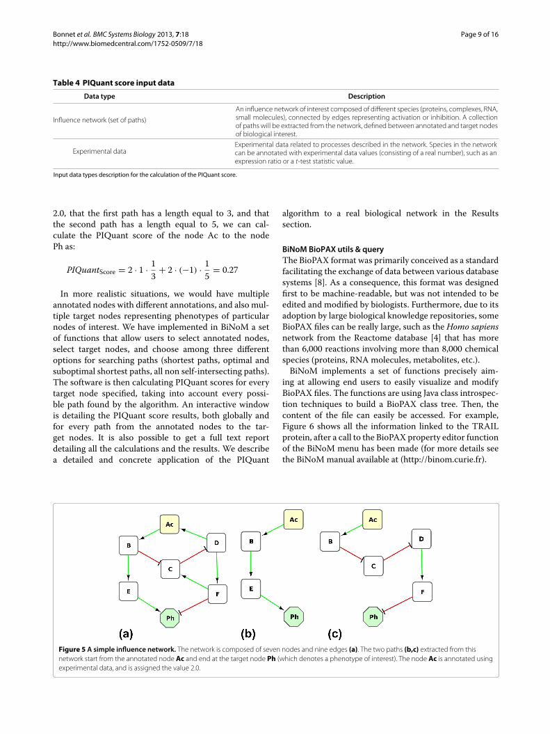
In the case of the network presented in Figure 5a, let us

consider Ac the annotated node and Ph the target node

and consider only the two paths defined in the Figures 5b

and 5c. Given that the node Ac is annotated by the value

Bonnet et al. BMC Systems Biology 2013, 7:18 Page 9 of 16

http://www.biomedcentral.com/1752-0509/7/18

Table 4 PIQuant score input data

Data type Description

Influence network (set of paths)

An influence network of interest composed of different species (proteins, complexes, RNA,small molecules), connected by edges representing activation or inhibition. A collectionof paths will be extracted from the network, defined between annotated and target nodesof biological interest.

Experimental dataExperimental data related to processes described in the network. Species in the networkcan be annotated with experimental data values (consisting of a real number), such as anexpression ratio or a t-test statistic value.

Input data types description for the calculation of the PIQuant score.

2.0, that the first path has a length equal to 3, and that

the second path has a length equal to 5, we can cal-

culate the PIQuant score of the node Ac to the node

Ph as:

PIQuantScore = 2 · 1 ·1

3+ 2 · (−1) ·

1

5= 0.27

In more realistic situations, we would have multiple

annotated nodes with different annotations, and also mul-

tiple target nodes representing phenotypes of particular

nodes of interest. We have implemented in BiNoM a set

of functions that allow users to select annotated nodes,

select target nodes, and choose among three different

options for searching paths (shortest paths, optimal and

suboptimal shortest paths, all non self-intersecting paths).

The software is then calculating PIQuant scores for every

target node specified, taking into account every possi-

ble path found by the algorithm. An interactive window

is detailing the PIQuant score results, both globally and

for every path from the annotated nodes to the tar-

get nodes. It is also possible to get a full text report

detailing all the calculations and the results. We describe

a detailed and concrete application of the PIQuant

algorithm to a real biological network in the Results

section.

BiNoM BioPAX utils & query

The BioPAX format was primarily conceived as a standard

facilitating the exchange of data between various database

systems [8]. As a consequence, this format was designed

first to be machine-readable, but was not intended to be

edited and modified by biologists. Furthermore, due to its

adoption by large biological knowledge repositories, some

BioPAX files can be really large, such as the Homo sapiens

network from the Reactome database [4] that has more

than 6,000 reactions involving more than 8,000 chemical

species (proteins, RNA molecules, metabolites, etc.).

BiNoM implements a set of functions precisely aim-

ing at allowing end users to easily visualize and modify

BioPAX files. The functions are using Java class introspec-

tion techniques to build a BioPAX class tree. Then, the

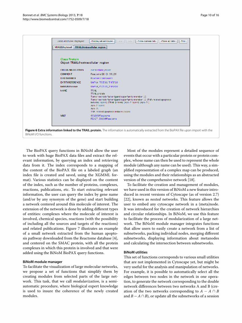
content of the file can easily be accessed. For example,

Figure 6 shows all the information linked to the TRAIL

protein, after a call to the BioPAX property editor function

of the BiNoM menu has been made (for more details see

the BiNoMmanual available at (http://binom.curie.fr).

Figure 5 A simple influence network. The network is composed of seven nodes and nine edges (a). The two paths (b,c) extracted from this

network start from the annotated node Ac and end at the target node Ph (which denotes a phenotype of interest). The node Ac is annotated using

experimental data, and is assigned the value 2.0.

Bonnet et al. BMC Systems Biology 2013, 7:18 Page 10 of 16

http://www.biomedcentral.com/1752-0509/7/18

Figure 6 Extra information linked to the TRAIL protein. The information is automatically extracted from the BioPAX file upon import with the

BiNoM I/O functions.

The BioPAX query functions in BiNoM allow the user

to work with huge BioPAX data files and extract the rel-

evant information, by querying an index and retrieving

data from it. The index corresponds to a mapping of

the content of the BioPAX file on a labeled graph (an

index file is created and saved, using the XGMML for-

mat). Various statistics can be displayed on the content

of the index, such as the number of proteins, complexes,

reactions, publications, etc. To start extracting relevant

information, the user can query the index by gene name

(and/or by any synonym of the gene) and start building

a network centered around this molecule of interest. The

extension of the network is done by adding different types

of entities: complexes where the molecule of interest is

involved, chemical species, reactions (with the possibility

of including all the sources and targets of the reactions)

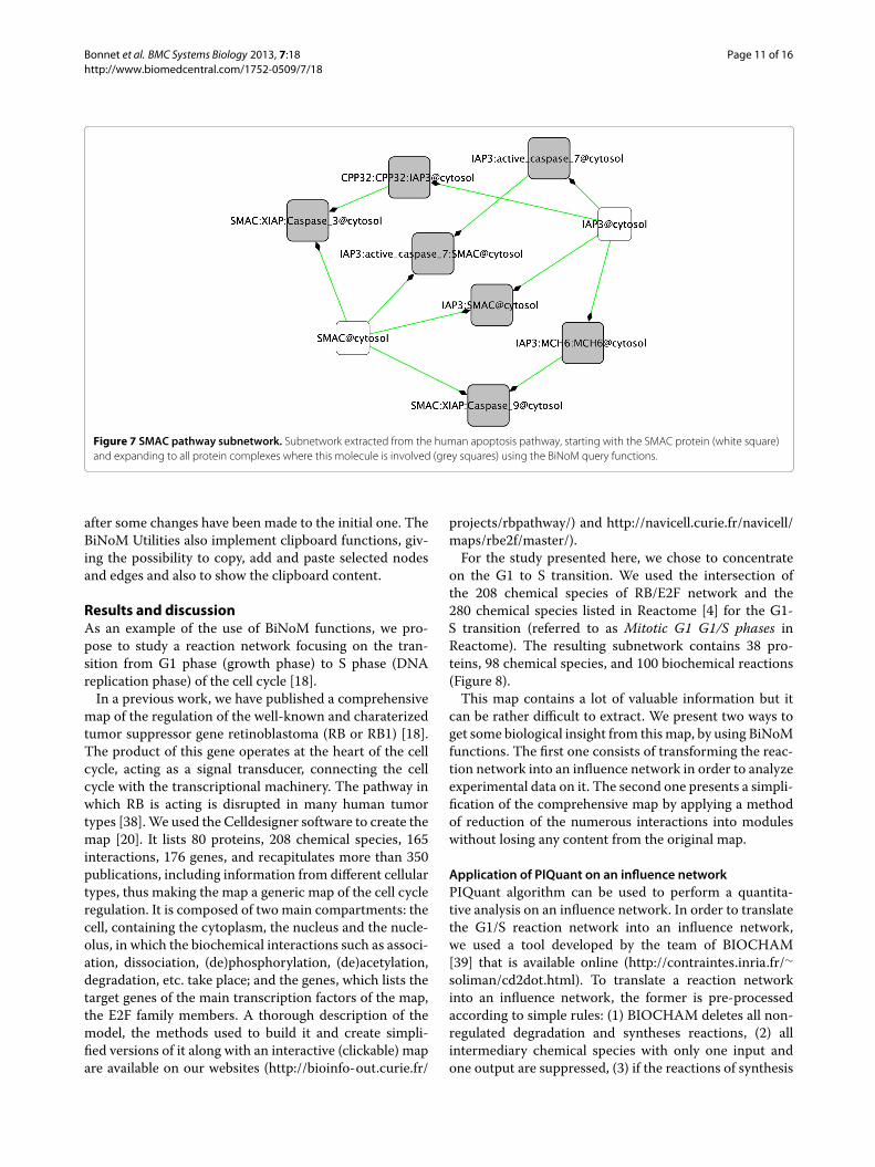
and related publications. Figure 7 illustrates an example

of a small network extracted from the human apopto-

sis pathway downloaded from the Reactome database [4],

and centered on the SMAC protein, with all the protein

complexes in which this protein is involved and that were

added using the BiNoM BioPAX query functions.

BiNoMmodule manager

To facilitate the visualization of large molecular networks,

we propose a set of functions that simplify them by

creating modules from selected parts of the large net-

work. This task, that we call modularization, is a semi-

automatic procedure, where biological expert knowledge

is used to insure the coherence of the newly created

modules.

Most of the modules represent a detailed sequence of

events that occur with a particular protein or protein com-

plex, whose name can then be used to represent the whole

module (although any name can be used). This way, a sim-

plified representation of a complex map can be produced,

using the modules and their relationships as an abstracted

version of the comprehensive network [18].

To facilitate the creation and management of modules,

we have used in this version of BiNoM a new feature intro-

duced in recent versions of Cytoscape (as of version 2.7)

[22], known as nested networks. This feature allows the

user to embed any cytoscape network in a (meta)node.

It was introduced for the creation of network hierarchies

and circular relationships. In BiNoM, we use this feature

to facilitate the process of modularization of a large net-

work. The BiNoM module manager integrates functions

that allow users to easily create a network from a list of

subnetworks, packing individual nodes, merging different

subnetworks, displaying information about metanodes

and calculating the intersection between subnetworks.

BiNoM utilities

This set of functions corresponds to various small utilities

that are not implemented in Cytoscape yet, but might be

very useful for the analysis and manipulation of networks.

For example, it is possible to automatically select all the

edges between two nodes in the network in one opera-

tion, to generate the network corresponding to the double

network differences between two networks A and B (cre-

ation of the two networks corresponding to A − A ∩ B

and B−A∩ B), or update all the subnetworks of a session

Bonnet et al. BMC Systems Biology 2013, 7:18 Page 11 of 16

http://www.biomedcentral.com/1752-0509/7/18

Figure 7 SMAC pathway subnetwork. Subnetwork extracted from the human apoptosis pathway, starting with the SMAC protein (white square)

and expanding to all protein complexes where this molecule is involved (grey squares) using the BiNoM query functions.

after some changes have been made to the initial one. The

BiNoM Utilities also implement clipboard functions, giv-

ing the possibility to copy, add and paste selected nodes

and edges and also to show the clipboard content.

Results and discussionAs an example of the use of BiNoM functions, we pro-

pose to study a reaction network focusing on the tran-

sition from G1 phase (growth phase) to S phase (DNA

replication phase) of the cell cycle [18].

In a previous work, we have published a comprehensive

map of the regulation of the well-known and charaterized

tumor suppressor gene retinoblastoma (RB or RB1) [18].

The product of this gene operates at the heart of the cell

cycle, acting as a signal transducer, connecting the cell

cycle with the transcriptional machinery. The pathway in

which RB is acting is disrupted in many human tumor

types [38].We used the Celldesigner software to create the

map [20]. It lists 80 proteins, 208 chemical species, 165

interactions, 176 genes, and recapitulates more than 350

publications, including information from different cellular

types, thus making the map a generic map of the cell cycle

regulation. It is composed of two main compartments: the

cell, containing the cytoplasm, the nucleus and the nucle-

olus, in which the biochemical interactions such as associ-

ation, dissociation, (de)phosphorylation, (de)acetylation,

degradation, etc. take place; and the genes, which lists the

target genes of the main transcription factors of the map,

the E2F family members. A thorough description of the

model, the methods used to build it and create simpli-

fied versions of it along with an interactive (clickable) map

are available on our websites (http://bioinfo-out.curie.fr/

projects/rbpathway/) and http://navicell.curie.fr/navicell/

maps/rbe2f/master/).

For the study presented here, we chose to concentrate

on the G1 to S transition. We used the intersection of

the 208 chemical species of RB/E2F network and the

280 chemical species listed in Reactome [4] for the G1-

S transition (referred to as Mitotic G1 G1/S phases in

Reactome). The resulting subnetwork contains 38 pro-

teins, 98 chemical species, and 100 biochemical reactions

(Figure 8).

This map contains a lot of valuable information but it

can be rather difficult to extract. We present two ways to

get some biological insight from thismap, by using BiNoM

functions. The first one consists of transforming the reac-

tion network into an influence network in order to analyze

experimental data on it. The second one presents a simpli-

fication of the comprehensive map by applying a method

of reduction of the numerous interactions into modules

without losing any content from the original map.

Application of PIQuant on an influence network

PIQuant algorithm can be used to perform a quantita-

tive analysis on an influence network. In order to translate

the G1/S reaction network into an influence network,

we used a tool developed by the team of BIOCHAM

[39] that is available online (http://contraintes.inria.fr/∼

soliman/cd2dot.html). To translate a reaction network

into an influence network, the former is pre-processed

according to simple rules: (1) BIOCHAM deletes all non-

regulated degradation and syntheses reactions, (2) all

intermediary chemical species with only one input and

one output are suppressed, (3) if the reactions of synthesis

Bonnet et al. BMC Systems Biology 2013, 7:18 Page 12 of 16

http://www.biomedcentral.com/1752-0509/7/18

Figure 8 G1/S network. Overview of the G1 to S transition network, corresponding to the intersection of RB/E2F network and G1/S network

extracted from Reactome.

and degradation of the chemical species deleted in (2)

have distinct inputs and outputs, then these reactions can

be merged, and (4) if they have the same chemical species

as input/output, then the reaction is a reversible reaction

and is replaced by a degradation [40]. A thorough descrip-

tion of the procedure together with an example of such a

conversion is available in [41].

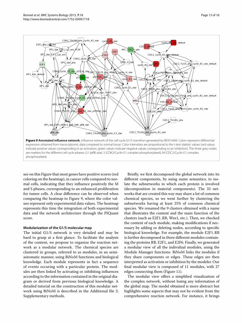
We applied PIQuant to the resulting influence network

of the G1/S transition of the cell cycle (Figure 9). We

selected three target nodes as markers of the G1, S and

M phases of the cell cycle. For the experimental data, we

used expression data from a study of 57 bladder cancer

tissue samples compared to 4 normal samples [42]. For

each gene, the differential expression between tumor and

normal tissue is assessed by a t-test. The t-test statistic

value is used as the annotation for each node. We selected

the 19 nodes for which we had experimental data values

as annotated nodes. Then, we constructed a text file list-

ing nodes of the influence network and their annotation

and we imported this file using the Cytoscape function

“Import > Nodes attributes” in the Cytoscape session of

the influence network. Figure 9 represents this influence

network after its import.

PIQuant is applied to this network and its annotation, by

using the function “Plugins > BiNoM 2.1 > BiNoM Anal-

ysis> Path Influence Quantification analysis”.We selected

the option “optimal and suboptimal shortest path” as the

algorithm to extract the paths. The PIQuant score is then

automatically calculated for each association between an

annotated node and a target node. The user can browse

the results on an interactive window detailing the different

paths and their scores, and can also get a complete report,

detailing the global and individual PIQuant scores from

each annotated node to each cell-cycle phase marker (for

more details on the interactive window and the report,

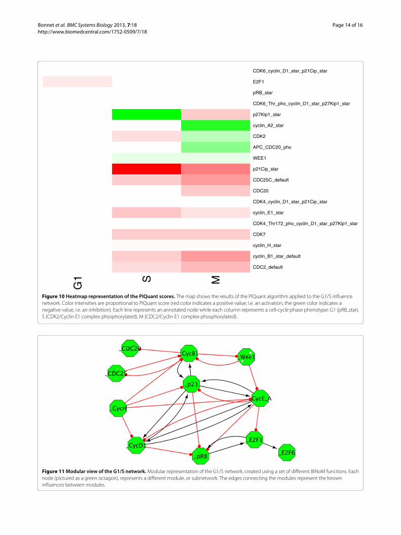
see the BiNoM manual). The global PIQuant score from

each annotated source node to each target is represented

as a heatmap on Figure 10 (the list of nodes and all

the PIQuant score values corresponding to the heatmap

Figure are available as Additional file 1: Table S1). We can

Bonnet et al. BMC Systems Biology 2013, 7:18 Page 13 of 16

http://www.biomedcentral.com/1752-0509/7/18

Figure 9 Annotated influence network. Influence network of the cell cycle G1/S transition generated by BIOCHAM. Colors represent differential

expression obtained from transcriptomic data compared to normal tissue. Color intensities are proportional to the t-test statistic values (red values

indicate positive values corresponding to an activation, green values indicate negative values corresponding to an inhibition). The three grey nodes

are markers for the different cell cycle phases: G1 (pRB star), S (CDK2/Cyclin E1 complex phosphorylated), M (CDC2/Cyclin E1 complex

phosphorylated.

see on this Figure thatmost genes have positive scores (red

coloring on the heatmap), in cancer cells compared to nor-

mal cells, indicating that they influence positively the M

and S phases, corresponding to an enhanced proliferation

for tumor cells. A clear difference can be observed when

comparing the heatmap to Figure 9, where the color val-

ues represent only experimental data values. The heatmap

represents this time the integration of both experimental

data and the network architecture through the PIQuant

score.

Modularization of the G1/S molecular map

The initial G1/S network is very detailed and may be

hard to grasp at a first glance. To facilitate the analysis

of the content, we propose to organize the reaction net-

work as a modular network. The chemical species are

clustered in groups, referred to as modules, in an semi-

automatic manner, using BiNoM functions and biological

knowledge. Each module represents in fact a sequence

of events occuring with a particular protein. The mod-

ules are then linked by activating or inhibiting influences

according to the information contained in the original dia-

gram or derived from previous biological knowledge. A

detailed tutorial on the construction of this modular net-

work using BiNoM is described in the Additional file 2:

Supplementary methods.

Briefly, we first decomposed the global network into its

different components, by using name semantics, to iso-

late the subnetworks in which each protein is involved

(decomposition in material components). The 33 net-

works that are created this waymay share a lot of common

chemical species, so we went further by clustering the

subnetworks having at least 25% of common chemical

species. We renamed the 9 clusters obtained with a name

that illustrates the content and the main function of the

clusters (such as E2F1 RB, Wee1, etc.). Then, we checked

the content of each module, making modifications if nec-

essary by adding or deleting nodes, according to specific

biological knowledge. For example, the module E2F1 RB

is further decomposed in three different modules contain-

ing the proteins RB, E2F1, and E2F6. Finally, we generated

a modular view of all the individual modules, using the

Module Manager functions. BiNoM links the modules if

they share components or edges. These edges are then

interpreted as activation or inhibition by the modeler. Our

final modular view is composed of 11 modules, with 27

edges connecting them (Figure 11).

The modular view offers a simplified visualization of

the complex network, without losing any information of

the global map. The model obtained is more abstract but

highlights some aspects that may not be evident from the

comprehensive reaction network. For instance, it brings

Bonnet et al. BMC Systems Biology 2013, 7:18 Page 14 of 16

http://www.biomedcentral.com/1752-0509/7/18

G1 S M

CDC2_default

cyclin_B1_star_default

cyclin_H_star

CDK7

CDK4_Thr172_pho_cyclin_D1_star_p27Kip1_star

cyclin_E1_star

CDK4_cyclin_D1_star_p21Cip_star

CDC20

CDC25C_default

p21Cip_star

WEE1

APC_CDC20_pho

CDK2

cyclin_A2_star

p27Kip1_star

CDK6_Thr_pho_cyclin_D1_star_p27Kip1_star

pRB_star

E2F1

CDK6_cyclin_D1_star_p21Cip_star

Figure 10 Heatmap representation of the PIQuant scores. The map shows the results of the PIQuant algorithm applied to the G1/S influence

network. Color intensities are proportional to PIQuant score (red color indicates a positive value; i.e. an activation, the green color indicates a

negative value, i.e. an inhibition). Each line represents an annotated node while each column represents a cell-cycle phase phenotype: G1 (pRB star),

S (CDK2/Cyclin E1 complex phosphorylated), M (CDC2/Cyclin E1 complex phosphorylated).

Figure 11Modular view of the G1/S network.Modular representation of the G1/S network, created using a set of different BiNoM functions. Each

node (pictured as a green octagon), represents a different module, or subnetwork. The edges connecting the modules represent the known

influences between modules.

Bonnet et al. BMC Systems Biology 2013, 7:18 Page 15 of 16

http://www.biomedcentral.com/1752-0509/7/18

into relief feedbacks (positive, negative, or feedforward)

involving the major players of the cell cycle, and prepares

the network for mathematical modeling. The transla-

tion of this modular network into a Boolean model, for

instance, is indeed straightforward. Another application

for the modular model would be to analyze experimen-

tal data such as transcriptome or copy number variations

(CGH). The “activity” of each module is based on the

expression levels of the genes within the module, which

can be visualized using a color code on the modular map.

It’s then fairly easy to analyze the difference between a

disease and a normal state, or even to try to discrimi-

nate between different disease stages. We have produced

such maps for the RB/E2F modular network to analyze

bladder tumor samples, and we could observe a striking

difference between the non-invasive and invasive states of

the disease [18] (the map and the details about the proce-

dure can be seen at (http://bioinfo-out.curie.fr/projects/

rbpathway/case study.html).

ConclusionsBuilding a useful model for systems and mathematical

biology is a multi-step process, beginning with the col-

lection of biological knowledge and progressing towards

the formalization of a network and its translation in math-

ematical terms. BiNoM is designed to help during the

intermediate steps of this process, by providing a conve-

nient access to a selection of standard systems biology

formats, by giving the possibility to analyze the network

using various graph theory algorithms and map biologi-

cal data onto it. BiNoM is clearly not a tool for numerical

simulations, but it provides functions to export final net-

works to the SBML and GINsim file formats (through

the GINsim Cytoscape plugin for Boolean modeling),

facilitating the import into various numerical simulators.

Together with functions described in this manuscript,

BiNoM implements several other methods which are

described elsewhere such as finding optimal minimal cut

sets (http://bioinfo-out.curie.fr/projects/ocsana/), color-

ing CellDesigner maps, creating Google Maps-based

interface for browsing large networkmaps (http://navicell.

curie.fr) and finding enriched subnetworks [43].

Availability and requirements• Project name: BiNoM• Project home page: (http://binom.curie.fr/)• Operating system(s): Platform independent• Programming language: Java• Other requirements: Java 1.5 or higher, Cytoscape

2.7, 2.8• License: GNU LGPL• Any restriction to use by non-academics: none

Additional file

Additional file 1: Table S1. PIQuant score values for all the annotated

nodes (rows) and all the target nodes (columns) of the G1/S influence

network.

Additional file 2: Supplementary methods. Installation procedure for

BiNoM, changelog for BiNoM version 2.0 compared to version 1.0 and

detailed tutorial for the creation of a modular view of the G1/S network

using BiNoM functions.

Competing interests

The authors declare that they have no conflict of interest.

Authors’ contributions

EB, AZ and LC designed the study. EB, AZ and DR wrote the code. EB, AZ, LC,

DR and GS generated the data, performed the analyses and interpreted the

results. EB, AZ and LC wrote the manuscript. AZ and EmB supervised the study.

All authors edited and approved the final version of the manuscript.

Acknowledgements

The research leading to these results has received funding from the European

Union Seventh Framework Programme (FP7/2007-2013) ASSET project under

grant agreement number FP7-HEALTH-2010-259348 and from the grant

“Projet Incitatif et Collaboratif Computational Systems Biology Approach for

Cancer” from Institut Curie. EB, LC, DR, GS, EmB and AZ are members of the

team “Computational Systems Biology of Cancer”, Equipe labellise par la Ligue

Nationale Contre le Cancer. The authors would like to thank the anonymous

reviewers for their valuable comments and suggestions.

Author details1 Institut Curie, 26 rue d’Ulm, Paris, F-75248 France. 2 INSERM, U900, Paris,

F-75248 France. 3Mines ParisTech, Fontainebleau, F-77300 France.

Received: 7 September 2012 Accepted: 11 February 2013

Published: 1 March 2013

References

1. Adriaens M, Jaillard M, Waagmeester A, Coort S, Pico A, Evelo C: The

public road to high-quality curated biological pathways. Drug Discov

Today 2008, 13(19-20):856–862.

2. Cary M, Bader G, Sander C: Pathway information for systems biology.

FEBS Lett 2005, 579(8):1815–1820.

3. Ogata H, Goto S, Sato K, Fujibuchi W, Bono H, Kanehisa M: KEGG: Kyoto

encyclopedia of genes and genomes. 27 1999:29–34.

4. Joshi-Tope G, Gillespie M, Vastrik I, D’Eustachio P, Schmidt E, de Bono B,

Jassal B, Gopinath G, Wu G, Matthews L, et al: Reactome: a

knowledgebase of biological pathways. Nucleic Acids Res 2005,

33(suppl 1):D428.

5. Zanzoni A, Montecchi-Palazzi L, Quondam M, Ausiello G, Helmer-Citterich

M, Cesareni G:MINT: a Molecular INTeraction database. FEBS Lett 2002,

513:135–140.

6. Saraiya P, North C, Duca K: Visualizing biological

pathwaysrequirements analysis, systems evaluation and research

agenda. Inf Vis 2005, 4(3):191–205.

7. Gehlenborg N, O’Donoghue S, Baliga N, Goesmann A Hibbs, M, Kitano H,

Kohlbacher O, Neuweger H, Schneider R, Tenenbaum D, et al:

Visualization of omics data for systems biology. Nat Methods 2010,

7:S56–S68.

8. Demir E, Cary M, Paley S, Fukuda K, Lemer C, Vastrik I, Wu G, D’Eustachio P,

Schaefer C, Luciano J, et al: The BioPAX community standard for

pathway data sharing. Nat Biotechnol 2010, 28(9):935–942.

9. Hucka M, Finney A, Sauro H, Bolouri H, Doyle J, Kitano H, Arkin A, Bornstein

B, Bray D, Cornish-Bowden A, et al: The systems biology markup

language (SBML): a medium for representation and exchange of

biochemical network models. Bioinformatics 2003, 19(4):524.

10. Le Novere N, Hucka M, Mi H, Moodie S, Schreiber F, Sorokin A, Demir E,

Wegner K, Aladjem M, Wimalaratne S, et al: The systems biology

graphical notation. Nat Biotechnol 2009, 27(8):735–741.

Bonnet et al. BMC Systems Biology 2013, 7:18 Page 16 of 16

http://www.biomedcentral.com/1752-0509/7/18

11. Bader G, Cary M, Sander C: Pathguide: a pathway resource list.

Nucleic Acids Res 2006, 34(suppl 1):D504–D506.

12. Karlebach G, Shamir R:Modelling and analysis of gene regulatory

networks. Nat Rev Mol Cell Biol 2008, 9(10):770–780.

13. Kitano H: Systems biology: a brief overview. Science 2002,

295(5560):1662–1664.

14. Ideker T, Galitski T, Hood L: A new approach to decoding life: systems

biology. Annu Rev Genomics HumGenet 2001, 2:343–372.

15. Bauer-Mehren A, Furlong L, Sanz F: Pathway databases and tools for

their exploitation: benefits, current limitations and challenges.

Mol Syst Biol 2009, 5(290).

16. Oda K, Matsuoka Y, Funahashi A, Kitano H: A comprehensive pathway

map of epidermal growth factor receptor signaling.Mol Syst Biol

2005, 1:2005.0010.

17. Oda K, Kitano H: A comprehensive map of the toll-like receptor

signaling network.Mol Syst Biol 2006, 2:2006.0015.

18. Calzone L, Gelay A, Zinovyev A, Radvanyl F, Barillot E: A comprehensive

modular map of molecular interactions in RB/E2F pathway.Mol Syst

Biol 2008, 4(174).

19. Caron E, Ghosh S, Matsuoka Y, Ashton-Beaucage D, Therrien M, Lemieux

S, Perreault C, Roux P, Kitano H: A comprehensive map of the mTOR

signaling network.Mol Syst Biol 2010, 6:453.

20. Funahashi A, Tanimura N, Morohashi M, Kitano H: CellDesigner: a

process diagram editor for gene-regulatory and biochemical

networks. BIOSILICO 2003, 1:159–162.

21. Zinovyev A, Viara E, Calzone L, Barillot E: BiNoM: a Cytoscape plugin for

manipulating and analyzing biological networks. Bioinformatics 2008,

24(6):876.

22. Cline M, Smoot M, Cerami E, Kuchinsky A, Landys N, Workman C,

Christmas R, Avila-Campilo I, Creech M, Gross B, et al: Integration of

biological networks and gene expression data using Cytoscape.

Nat Protoc 2007, 2(10):2366.

23. Mi H, Muruganujan A, Demir E, Matsuoka Y, Funahashi A, Kitano H,

Thomas P: BioPAX support in CellDesigner. Bioinformatics 2011,

27(24):3437–3438.

24. Buchel F, Wrzodek C, Mittag F, Drager A, Eichner J, Rodriguez N, Le Novere

N, Zell A: Qualitative translation of relations from BioPAX to SBML

qual. Bioinformatics 2012.

25. Ruebenacker O, Moraru I, Schaff J, Blinov M: Integrating BioPAX

pathway knowledge with SBMLmodels. Syst Biol, IET 2009,

3(5):317–328.

26. Konig M, Drager A, Holzhutter H: CySBML: a Cytoscape plugin for

SBML. Bioinformatics 2012, 28(18):2402–2403.

27. Su G, Kuchinsky A, Morris J, Meng F, et al: GLay: community structure

analysis of biological networks. Bioinformatics 2010, 26(24):

3135–3137.

28. Bader G, Hogue C: An automated method for finding molecular

complexes in large protein interaction networks. BMC Bioinformatics

2003, 4:2.

29. Szalay-Beko M, Palotai R, Szappanos B, Kovacs I, Papp B, Csermely P:

ModuLand plug-in for Cytoscape: determination of hierarchical

layers of overlapping network modules and community centrality.

Bioinformatics 2012, 28(16):2202–2204.

30. Morris J, Apeltsin L, Newman A, Baumbach J, Wittkop T, Su G, Bader G,

Ferrin T: clusterMaker: a multi-algorithm clustering plugin for

Cytoscape. BMC Bioinformatics 2011, 12(436).

31. Rivera C, Vakil R, Bader J: NeMo: network module identification in

Cytoscape. BMC Bioinformatics 2010, 11(Suppl 1):S61.

32. Gonzalez A, Naldi A, Sanchez L, Thieffry D, Chaouiya C: GINsim: A

software suite for the qualitative modelling, simulation and analysis

of regulatory networks. Biosystems 2006, 84(2):91–100.

33. Tarjan R: Depth-first search and linear graph algorithms. SIAM J

Comput 1972, 1(2):146–160.

34. Broder A, Kumar R, Maghoul F, Raghavan P, Rajagopalan S, Stata R,

Tomkins A, Wiener J: Graph structure in the web. Comput Netw 2000,

33(1-6):309–320.

35. Novak B, Csikasz-Nagy A, Gyorffy B, Nasmyth K, Tyson J:Model scenarios

for evolution of the eukaryotic cell cycle. Philos Trans R Soc Lond B Biol

Sci 1998, 353(1378):2063.

36. Gleiss P, Stadler P, Wagner A, Fell D: Relevant cycles in chemical

reaction networks. Adv Complex Syst 2001, 4(2/3):207–226.

37. Vismara P: Union of all the minimum cycle bases of a graph. Electr J

Comb 1997, 4:73–87.

38. Weinberg R, et al: The retinoblastoma protein and cell cycle control.

Cell 1995, 81(3):323–330.

39. Calzone L, Fages F, Soliman S: BIOCHAM: an environment for

modeling biological systems and formalizing experimental

knowledge. Bioinformatics 2006, 22(14):1805–1807.

40. Fage F, Soliman S: From reaction models to influence graphs and

back: a theorem. Formal Methods Syst Biol FMSB’08, Lect Notes Comput Sci

2008, 5054:90–102.

41. Calzone L, Chaouiya C, Remy E, Soliman S: Qualitative modelling of the

RB/E2F network, deliverable D3.1. ANR CALAMAR (ANR-08-SYSC-003)

2011. [Https://tagc.univ-mrs.fr/welcome/IMG/pdf/livrable-3-1.pdf].

42. Stransky N, Vallot C, Reyal F, Bernard-Pierrot I, de Medina S, Segraves R,

de Rycke Y, Elvin P, Cassidy A, Spraggon C, et al: Regional copy

number–independent deregulation of transcription in cancer.

Nature Genet 2006, 38(12):1386–1396.

43. Kairov U, Karpenyuk T, Ramanculov E, Zinovyev A: Network analysis of

gene lists for finding reproducible prognostic breast cancer gene

signatures. Bioinformation 2012, 18(6):773–776.

doi:10.1186/1752-0509-7-18Cite this article as: Bonnet et al.: BiNoM 2.0, a Cytoscape plugin for access-ing and analyzing pathways using standard systems biology formats. BMCSystems Biology 2013 7:18.

Submit your next manuscript to BioMed Centraland take full advantage of:

• Convenient online submission

• Thorough peer review

• No space constraints or color figure charges

• Immediate publication on acceptance

• Inclusion in PubMed, CAS, Scopus and Google Scholar

• Research which is freely available for redistribution

Submit your manuscript at www.biomedcentral.com/submit