Biochemical Engineering Prof. Dr. Rintu Banerjee ...textofvideo.nptel.ac.in/103105054/lec26.pdf ·...

Biochemical Engineering Prof. Dr. Rintu Banerjee

Department of Agricultural and Food Engineering Prof. Dr. Saikat Chakraborty

Department of Chemical Engineering Indian Institute of Technology, Kharagpur

Module No. # 01 Lecture No. # 26

Design of Bioreactors

Today, we start a new chapter on design and analysis of bioreactors, and this chapter, in a

way brings together, you know, much of what we had done in the last part of the course.

And, the reason I am saying that, it brings together much of what we have done in the

last part of the course because, we had looked at fundamental processes. So, we looked

at the kinetics of enzyme; we had looked at the effect of mass transfer and that kinetics;

we had looked at growth, cell culture and cell growth; we had looked at the effect of

mass transfer and cell growth; we had looked at the effect of inhibition and so on, you

know, on, on cell growth inhibition and a multiple substrates and so on and so. But, these

are all fundamental processes, we look, we looked at. But, what happens to these

fundamental processes when we bring them together into a real system, and that is a

thing that we are going to study.

So, what is the real system? Because you are, if you are trying to culture a cell, you

would need, on a, on a large scale, you would need a bioreactor. Now, the bioreactor

could be, either a batch type of reactor, where you put in the stuffs and let it be there for

a day. So, put in the stuff, we put it, put in the cell that you, excuse me, cells that you

need to, that you are trying to incubate, put in the nutrients, allow it to stay there for a

day or so, and then, you generate the products; so that, it could be a batch system; or, it

could be a continuous system, that is, the feed, that is a nutrients and the cell is coming

in, and it is going out at a continuous rate. Now, that continuous rate could be a very

slow rate, you know. So, the resting time in the system of the reactor could be of hours

and could be of, of the order of a day even; it could be a very slow rate; but still, you can

have a continuous system. So, these are the two different kinds of bioreactors that we are

going to talk about. But, what I am trying to say is that, these bioreactors bring in all the

fundamentals, bring in the kinetics, the cell growth kinetics, the effect of inhibition,

effect of substrates and so on. So, excuse me. So, as a result, what happens is that, any

real system, when it brings in all the complicated kinetics and everything, turns out to be

a little more complicated than the fundamental systems that we had studied. So, as a

result, this is slightly more complicated, than what we had done before. Today’s lecture

is going to be straightforward and simple. It is on just the design of bioreactors, but,

when we go into the analysis of bioreactors, you will see, because of this different factors

coming in, for example, the substrate and the, and the cell concentration, and that we, we

have not, we may or may not even look at the effect of inhibition; but, when we do it, it

is a lot more complicated; the effect of inhibition, the multiple substrates, because of all

of these, coming in at the same time, in a real process.

Till now, we are looking, as I said, we are looking at only kinetics, or mass transfer, as

the, as, as a theme, or a subject, to study; just as something of theoretical interest; but

now, we are, we are trying to understand something, which is of engineering interest and

this is a very engineering aspect of the course, where we are trying to understand and

quantify, how much cells are going to be produced and what is the amount of substrates;

very basic things; what is the amount of substrates that we, I need to put? What is the,

how much cells are going to be produced? What it should be the size of the reactor? You

know, what should be the resistance time in the reactor? In other words, what should be

the size of the reactor? If it is a batch reactor, what should be the time we should give?

These are questions that we will try to address and those will be coming in the analysis

part, starting from the following lecture.

(Refer Slide Time 03:53)

Today’s lecture, as I said is straightforward, and let us start it. It is called design and

analysis of bioreactors. As I said that, the two kinds of reactors we are going to look at;

our batch reactor and C S T R, Continuous Stirred Tank Reactors. And, the stirring, you

know, has to be slow, because, you do not want very high stirring rate in these reactors

with cells. So, if you write a batch reactor, you have studied batch reactors before. So, if

you write a batch reactor, what would be the balance of batch reactor? What kind of

balances you, you need to write? You just…

(( )).

What is that?

(( )).

It is just a volume balance and the product, one for the concentration of the products. So,

this is, this is the balance for the concentration of the product, as you can see over here.

So, d d t of c i times V. is V times r, r being the reaction rate, and r is the function of c i

and c j, that is all components, fine. Now, my V is the constant out of that. So, if they,

when it is going, it is going to be a constant? It is going to be a constant, if it is a liquid

phase reaction, because, liquid phase reactions, typically do not change volume much;

even if they change because of molar increase, it is not appreciable. So, if V, volume is a

constant, then, you can take it out of the differential and cancel it, and you will get, d c d

t equals r of c. So, this is the total volume balance. So, this is the balance for the

particular components c i, and this is the total volume balance, rho being the density. For

a constant volume-constant density system, this, you know, whole term would be 0 and

you will, can take V out of the system.

So, this is for liquid reactions, or constant volume-constant density systems. Typically,

more or less constant volume and actually, constant density systems. So, you can take it

out of the differential, and you can write, d c d t equals r of c, right. And then, you can

add in a thermal energy balance if you want, which is, if the temperature of the system is

changing appreciably. Typically, it does not change appreciably, the reason being, you

know, there is a, there is a range of temperature within which the system has to be

maintained, and you try to maintain it typically within a small range. Within that small

range, the changes are not large, and another, the, the reason the changes are not large

because, these growth reactions that take place, do not have a very high activation

energy. And, they do not really have, the heat of energy is not really very high.

So, typically, we neglect the thermal balance, but, if, to be on the safe side, and to be,

you know, theoretically very correct, if you want to write a thermal balance, then, this is

how it looks like; rho times v times C p and d T d t; so, rho being the density over here;

V being the volume of the reactor; C p being its specific heat of the mass of, you know,

whatever is there in the reactor, the liquid, average specific heat, T being the temperature

and little t being time; minus delta H r is the heat of reaction of the growth reaction that

is occurring. So, these are essentially, you know, any kinds of reactions, r could be any

kind of reaction, but, what we are looking at essentially is, are, growth reaction. So, we

are trying to culture cells over here, r being the reaction rate for the, for the rate of

culture; V is again the volume; Q is, is any kind of heat source, or sink, that could be

there in the reactor, apart from, apart from what is, you know, happening in the reactions.

So, apart from the heat of reaction, if there is the, any other kind of heat source or sink

inside the reactor, Q is that, and W is the work done by the reactor. This basic

thermodynamics model, I am sure, all of you are aware of.


Now, the reaction rate. So, we had the reaction rate over here, r, and what should be the

reaction rate? Now, as I said that, these equations are very basic equations and you can

use them for all kinds of reactions that happen in bioreactors, but, we want to specifically

look at, we have to specifically interested in growth reactions and we will use today, the

very simplest kinetics of growth, Monod kinetics; and through much of this chapter, we

are going to use Monod kinetics. But, you should be, you know, ready to deal with other

kinds of kinetics, because, in the test, that is what I might give you; you know, with

inhibition, like we did, with inhibition, with multiple substrates. So, what happens when

you put these kind of kinetics? It is gets lot more complicated, the whole analysis, and

you should be ready to do, do those kind of things; I, I tell you in advance. So, the

Monod growth models. So, you know, you are aware of the Monod growth models. So, d

x d t is mu X times mu, mu, mu x, where mu X is, mu is given as mu max time S over k

S plus S.

Now, let me ask you this, is this, is this equation that I wrote for the Monod growth

model, is this valid for all kinds of reactors? del x del t, whatever is on the screen, del x

del t equals mu X, is that valid for all kinds of reactors, or is it valid for a specific kind of

reactor?

(( ))

Resistance time is very large, no. In the limit of resistance time going to infinity, this is

valid; not very large, but, that is a too theoretical answer. Why you do not give a more

practical answer? That is correct, but, that is a very theoretical answer. Why do not you

give a very, more practical answer to that? When is that valid? When is…Is it valid for…


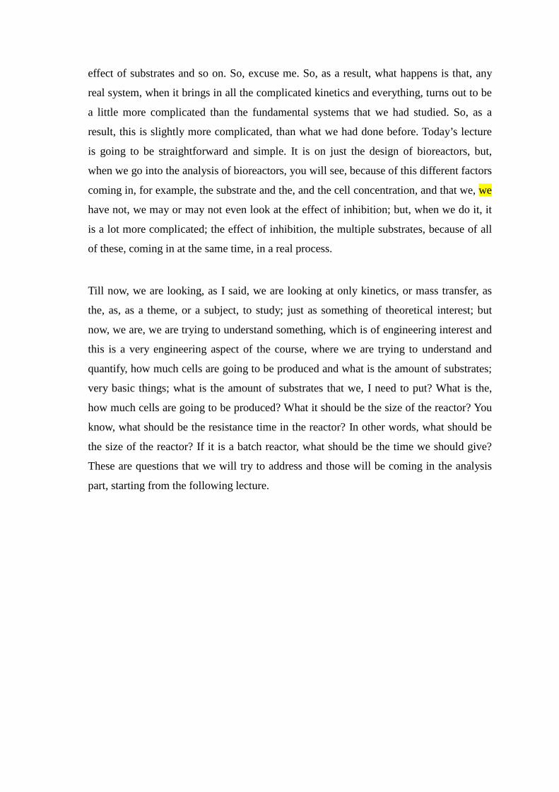
See, for the kind of reactors we are used to, are, let me, let me go through this a little bit,

and I wish, you know, I had. So, batch reactors, I think, this is the interesting thing I

would do; I did not bring all the details of the notes. So, reactor types, then is…Then…

So, these are the four reactors types you are aware of. Now, what I want you to tell me is

that, I am not sure if you know, but, you can make a try that, which, out of these four,

which was the first reactor that was discovered?

(( ))

Batch reactor; when was it discovered?

(( ))

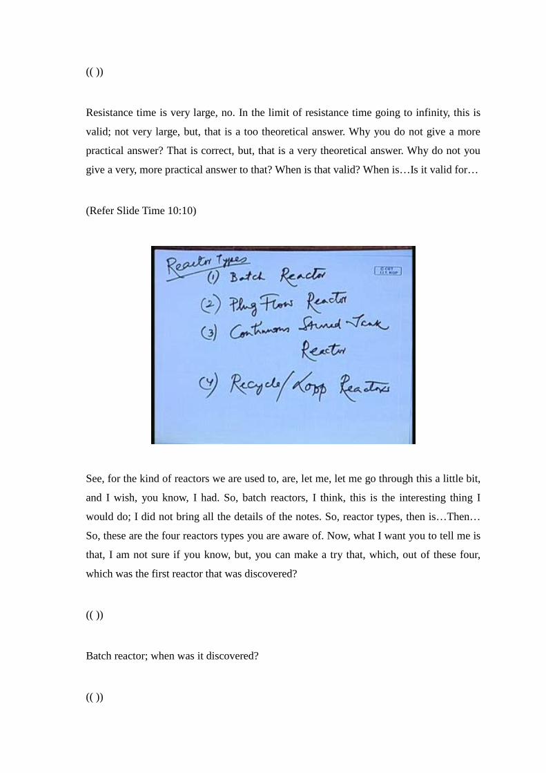
Well, the batch reactor was the first reactor to be discovered, that is true; but, it was

discovered at, not at 1800; it was discovered at the beginning of the human civilization;

you know, cooking, for example, is a batch reaction. So, if you think that way, and, so,

there is no account, exact account of when the batch reactor was discovered, because

everything that had been there, had been a batch process, till now. So, the batch reactor is

the most common, most natural of human reactors that had been used all through,

through the whole of human civilization. As I said that, you know, fermentation came in

much later; cooking is the, the very basic human activity, that started at the dawn of

human civilization, is, is essentially, a batch reaction that occurs, right. So, that is true

that, you know, batch reactor was in this around.


So, let us say, history of reactors. Batch reactor was, you know, sort of dawn of

civilization. The second one is a plug flow reactor, PFR; this is how we will refer to the

plug flow reactor. This was developed in the early years of the twentieth century. So, 19

around 1900, just after 1900; just after 1900; I think, 1905 or something like that; do you

have any clue, who could have discovered the plug flow reactor? It was discovered by,

any guess?

(( ))

Yes, discovered by Langmuir. Forget the year, around 1905 or something like that, 5 to 8,

I think, around 1908 or something. Langmuir is the first and only chemical engineer to

get Nobel; he is the first and only chemical engineer to get the Nobel prize. What did he

get the Nobel prize for, do you know?

(( ))

Langmuir-Hinshelwood isotherm, yes, Langmuir isotherm. So, for, but, he was the one

who, who discovered this. Now, the plug flow reactor was useful, you know, again, why

was that useful, because, till then, processes are batch; which means that, you put the

main and you know, wait for 4 hours, 6 hours and 12 hours, 24 hours to get the output.

So, which mean, meant that, during the entire process, you got no output; but, the plug

flow reactor was a first of continuous reactors, where you put things in at one end and

you got things out at the other end; which means that, we had continuous supply of

products, and that was necessary at the…And, this is, you know, even before the

beginning of the industrial age. So, this was just, just before the beginning of the

industrial age. And so, then, what happened was, the C S T R was discovered. C S T R

was discovered little after that, and that became a big breakthrough in whole of chemical

reaction engineering.


The discovery of C S T R. So, C S T R discovery was done by two German scientists

Bodenstein and Wohlgast and I forget the year; I think it was around 19; again, I think

1908 or 1909, something like that; just, just around, I will, I will give you the years in the

next class. I do not remember the, the year exactly. So, two German scientists, they were

the one who discovered the C S T, the C S T R. Now, this was published, Langmuir's

paper, I remember, was published in a Journal of American Chemical Society in 1908, I

think, I remember the journal; I will give you the, all this references; I have these

references with me, and I will give you those, those in next class and you can have a look

at that. So, Bodenstein and Wohlgast discovered the C S T R model and that was quiet a

breakthrough. The reason that was a breakthrough is that, you know, plug flow reactors

are not always very useful, because, they are long and pipe kind of things. So,

essentially, you know, a pipe kind of thing. And the problem with plug flow reactors is,

you can, you do not have much control over the reactor; at least, not in those times. What

it meant was, you only had control of what was going in and you did not really have

control over what was happening inside; whereas, a C S T R is like a chamber, but, you

just allow things to enter and take out. So, you have a continuous supply of products; you

have continuous input of reactants and you have a lot of control on the system, because,

you can stir it and you know, raise temperatures, decrease pH; do whatever you want to

do to the system. So, C S T R model was a huge breakthrough and I am not sure, if this is

1909, but, around that time, Bodenstein and Wohlgast model. So, that, that was a huge

breakthrough.

Now, what happened was that, this and this discovery of Bodenstein and Wohlgast was

kind of, you know, did not come out to the Western world, alright. It, it did not come out

to the English speaking world, alright; the reason being, this paper was published in

German and it was not translated at that point of time and people did not get to know

about this. So, this, there was a lot of obscurity that, this really happened and lot of other

people tried to take credit for this; but, that the, that was, that was not correct and then,

DamKohler also, you know, a kind of took, he is not directly, but, he was sort of, sort of

trying to take credit for the C S T R model. But, the model was first discovered by

Bodenstein and Wohlgast and that is kind of well known.

Now, the fourth thing, the important thing is not the loop and the recycle reactor models,

but, something related to it. It is the three dimensional Convection Diffusion Reaction

model. So, this is very important, also. The reason this is important is, this, the, the, this,

you know, the way we write the convection diffusion reaction model now, including the

diffusion terms, the reaction terms and the convection of the velocity terms out there, it

was a matter of discovery. If you come to think of it, it did not drop from heaven.

Somebody had to discover it, and that was the path breaking discovery in chemical

engineering as well; in, in the whole of science as well, because, that was the first time,

somebody showed that, it is not enough do some, you know, these, these are good

practical models, the C S T R model and the P F R model; but, that was not enough. It

was important to figure out, what are the basics of, of the model; what really goes into it

and where the, how does the convection term combined with the diffusion term and the

reaction term and so on. And, the person who did it is very famous scientist. He is a

German again, and can you, can you, do you have any idea? Let us, let we try, what you

think.

(( ))

Yes. So, I think, this was in, I have forgotten the year, but, with, this was in 1937 and this

was a breakthrough paper, paper, you know, this DamKohler’s paper. And, this was again

written in German and I am, I had a copy of this; I had a paper copy of this translated

into English by one of my friends; he is a German scientist. And, so, this is the

breakthrough paper, one of the greatest papers ever written in chemical engineering. The

reason is that, what he does, he reviews the whole history of Chemical Engineering,

DamKohler in 1937. And, he was the one, you know, who gave credit to Bodenstein and

Wohlgast. He brought the, brought C S T R model into light. So, that… So, the C S T R

model actually was discovered much before that, but, it was DamKohler who brought

this into light, one more time, and, it was kind of lost. And then, he talked about the 3 D

convection diffusion reaction model. He talks about simplifications of it. He showed,

how the P F R model actually comes out of the 3 D convection diffusion reaction model

under certain circumstances; a certain assumptions of axial diffusion, you know,

negligible and so on. So, this was a breakthrough paper. The DamKohler's paper in 1937

was one of the greatest papers ever written in chemical reaction engineering and is a

great review of everything that was going on. And, you know, so, he talked about the

axial dispersion model; not just C S T R model, the axial dispersion model also.


And then, I think, Danckwerts. Then, Danckwerts, you know, he is one of the greatest

known chemical engineering scientist. So, Danckwerts, we probably use Danckwerts

boundary conditions a lot. So, Danckwerts boundary conditions is cited to 1951 or 52,

something like that; 1951 say, to Danckwerts, but, it is essentially, was not developed by

Danckwerts. It is now, now, it is clear, because of the, we have reviewed the history of it.

And, it was first developed by Langmuir in 1908, in the A C S paper and then, by

German, some German scientists like Bodenstein and Wohlgast, and then, again by

DamKohler. So, this was shown again and again. So, Danckwerts boundary condition is,

Danckwerts used to take lot of credit for this, Danckwerts boundary condition, but, it has

now been shown that, the Danckwerts boundary condition was not found by Danckwerts

and I can give you the exact years. I will bring the data in the next class. So, we would

no longer call it the Danckwerts boundary condition; we just call it the flux type

boundary condition.

So, it was, there is a lot of credit given to Danckwerts, because that, again, boundary

condition was a path breaking thing; though we do not have, one thing you must know

that, we do not have Danckwerts boundary condition or 2 D, two dimensional or three

dimensional problems in the 3 D convection diffusion reaction model here. So, we have

the 3 D convection diffusion reaction model and we are not aware of what the entrance

boundary condition, flux type entrance boundary condition for the three dimensional

system is. Till now, we are not aware of; but, what we are aware of is, if you write a 1 Ds

model of this or a 2 D model of this, how to write the in boundary conditions. Because,

what happens in a 3 D is, because, as soon as you take the reactor like this type, this is

the reactor cross section and it goes like this. So, as soon as this 1 D or 2 D, it is all fine;

but, as soon as this theta dimension comes in like this, this whole boundary condition can

change; because, there could be a lot of effects of the theta direction. So, we are still not

aware; but still, this, this was a breakthrough condition, the flux type boundary

condition.

The reason that it was the breakthrough condition was, minus minus d del c, this is

boundary condition, right, equals, v times c minus c naught, like this, or, c minus c. That

what, what this said was that, whatever is coming in at the entrance, whatever is coming

in, because of…What is the, what is the flux type boundary condition mean? It says that,

whatever is coming in at the entrance, because of convection, equals what goes in,

because of diffusion plus convection, right. So, that is the boundary condition. See, if I,

if you look over here, then, you get minus c del c del x plus… So, if you put a plus over

here, then, plus V times C in equals V times C in; yes, this is, yes, just take this form. So,

this is what, this is what is coming in, V times C in, the velocity times concentration; I

am going to pull this a little to the middle, yes; this is what is coming in to the system

and what is going out is, diffusion plus convection, fine. So, this is the…So, there should

not be any confusion about this, because, this is the very straightforward system. So, this

is the, this is the boundary condition we have, the Danckwerts boundary condition. So,

essentially… So, I will do a review, a little bit of more review of what is going on in the,

in the, in this system, for the reactors; but, but, what I wanted to tell you is that, you

know, there are these four different kinds of reactors.


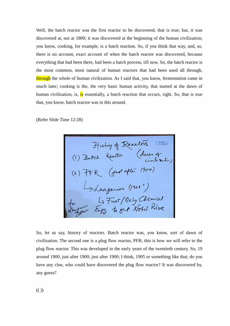
Let me bring that page one more time, yes. So, there is a four different kind of reactors,

the batch reactor, the plug flow reactor, the continuous stirred tank reactor, and the loop

reactor. And, there is a certain history to it and as I said, this is the earliest reactor, the, at

the dawn of human civilization. The plug flow reactor was around 1900; little before that

also, may be 1800 and so on, before the start of the industrial age. The Continuous

Stirred Tank Reactor was a huge breakthrough because, most of the industries shifted to

the Continuous Stirred Tank Reactor, because of what, of, of the advantages of it. It was

smaller; it was easy to handle; it was easy to control, easy to manipulate, and still you

have a continuous product and a supply of products. And then came the recycle or the

loop reactors. Can you tell me that, where are these recycle or loop reactors most used?

Which kind of industry?

(( ))

Yes, that is one and what else?

(( ))

Yes. So, this is actually, recycle, loop is not used so much in a effluent treatment, and the

recycle is used in effluent treatment, and loop is used in polymerization.


So, do you know the difference between the loop reactor and a recycle reactor? So, the

recycle reactor is something like this. So, you have the, this is the reactor, say, your main

reactor; this is going out and this is the recycle; recycle ratio is r, say; this is the recycle

reactor, clear. Something going out, things, things coming in, things going out, and there

is a, the, there is, there is a recycle out here. And, loop reactor is little different. This is

how it is. So, this is my reactor and this is the entrance, this is the exit. Do you see the

difference? You see the difference between the loop reactor and the recycle reactor, the

difference and the similarity. Similarity is that, things are being recycled in both cases,

but, in a recycle reactor, the reactor is not, reactor is one straight thing and there is a little

recycle going out; in the loop reactor, the reactor itself is a recycle. So, the major part of

it, what is the major difference? In the recycle reactor, only a small fraction is being

recycled; here, in the loop reactor, a large fraction is being recycled. Now, that would not

work with this kind of setup. If you want to recycle a large fraction of it, that would not

work with this kind of setup. So, you want to recycle a large fraction of it, you, you, you

put this kind of setup, where the, everything goes around in loops and loops. You put in

a, put in a little bit in, take a little bit out, but, rest of the things goes in again and again.

Why are these recycle and loop reactors used especially for reactions which are very…

(( ))

No, that is, that is not the point.

(( ))

Yes, reactions which are very slow, or low conversion reactions, so that, you tend to send

them again and again and again to make, make it work.

So, these are the different kinds of reactor that we use. And again, you know, for

biological systems, we can use all of these reactors, batch and plug flow and continuous

and even recycle reactors; there is no, nothing stopping us from doing the same thing;

but, when you use something like a recycle reactor, it is little hard, because, you have the

cells within it and you, it is hard to recycle with the cells, without killing the cells; you

know, slightly hard, but, you can. So, these are, in biological system, these continuous C

S T Rs are called chemostats, and batch reactor is called the batch reactor and the plug

flow is, is my…So, what I will do is, with this, history is interesting, but, I, I do not have,

I did not remember that, I should give the history to depth. So, I do not have all the

years. So, I will do quick review of the history in the next class and give you all the exact

dates and the papers; you know, I, I have the citations to all the papers that were being

written, and, and it is very interesting to be aware of the history of a process that we are,

you know, part of. Because, unless, I think, this is something you probably, you are not

aware of, what the history of these reactors are. So, there is a Danckwerts boundary

condition; then, there is the axial dispersion model and you, you know, and you are also

aware of the, of the surface renewal theory, right. So, surface renewal theory. So, that,

there is a history to that also. Anyway, so, these are some of the things, I will quickly

discuss in the next class.


So, let us go back to what we were doing, without the, you know, that was the creation, I

think. So, what we are doing is the Monod model and what I asked you is that, that, this

is where it started, is, are these, these are Monod growth model. Let us forget this; just

look at this. So, d x d t equals mu X, that is my Monod growth models for X. What I

asked you is, is this equation valid for all kinds of reactors and that is why, I digressed

and started talking about different kinds of reactors. What, which kind of reactor is this

model valid for? The way I have written it here, you should be able to tell this now.

(( ))

What about other reactors?

(( ))

Yes, because the batch reactor is the only kind of reactor which does not have a, which is

not a continuous reactor. So, if you, if you have a continuous reactor, and obviously, they

are going to be, there have to be input and output terms; so, the, it cannot, d x d t cannot

be written in just a reaction rate. So, this is something I want you to be very clear, that…

So, when it is a batch reactor, because, I see, see students keep doing it, despite telling

them again and again. So, d x d t equals to reaction rate, only and only for a batch

reactor; for all other kinds of reactors, d x d t is not just reaction rate, but, there are

inputs and output terms that has to be added in. So, do not ever write d x d t equals

reaction rate, unless it is a batch reactor, fine. So, this, this is, I mean, I tell students, but,

I still keep seeing these mistakes on the answer sheets; so, very straightforward thing,

but, you still need to remember it. So, in similar way, we can write the growth model, the

d x d t; this is again for batch reactor, for the substrates. So, X is my cell and S is my

substrate and the reaction rate is the same over here, except, there is a negative term

outside, because substrate is being consumed in the reaction; whereas, cells are being

generated and why is this Y x s, because, we discussed this in the last class, Y is the, Y is

the yield of X per unit mole of S. So, here, we have used this as the, this is my yield, you

know, reaction rate for X. So, you have to covert that into S; if you are doing molar

balance for S, then, the yield of X per unit volume of S, if that is Y, then, 1 over Y is the

yield of S per unit X, right. So, you just multiply it, that by that number, fine.

So, the, this is my basic equation for a batch reactor, and what we are, what we are doing

now is that, we try to express X in terms of S. So, when we, when we try to do that…So,

what do you see over here? You know, how do I, if I ask you to manipulate this system,

how would you do that? Tell me quickly. If this two equations are there, forget it, you

know, forget this; if I ask you to manipulate, so that, you get X in terms of S, how, how,

what would be the first step? I, I discussed this in this earlier, in earlier, in this lecture, I

think, when we were doing enzymes; there is something called method of invariants;

what is that? (( )).



So, my d x d t…

(( ))

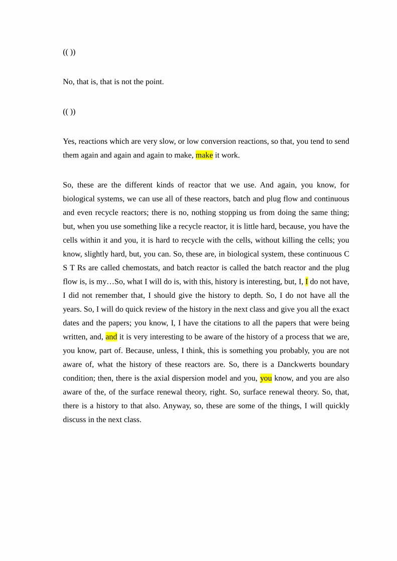
Yes, no; do not divide it; you just use, what is known as method of invariants. So, d x d t

equals mu X; d s d t equals minus 1 over Y times mu X. So, what you do is, multiply that

first equation by Y, multiply by Y and then, add, fine. So, multiply, now, sorry, multiply

this equation by Y and then, add. So, then you get, d x d t plus Y times d s d t equals 0, Y

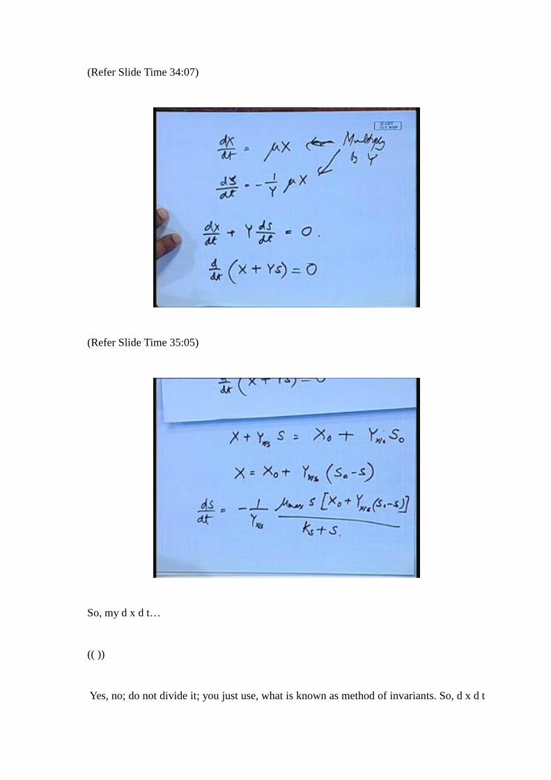
being a constant, fine. So, d d t of X plus Y S equals 0, fine. Then what? So, X plus Y x

over s times S equals X 0 plus Y x over S 0. Now, if there is no, I think, what we are

using here, yes, we still have X 0 here; so, then, X could be expressed as X 0 plus Y x

over s S 0 S, fine. So, my d s d t can be now written as minus 1 over Y x over s mu max

X 0 Y x over s S 0 minus S. So, that is fine and though this is non-linear, we can still

integrate it, because, it looks like, we can use partial fractions to integrate this, right;

appears to me, because, and just quadratic on the numerator and linear on the

denominator. So, I think, you can use partial fractions (( )) fine. So, this is called the,

what is this called? This is called the method of invariants, and you should not forget

this, because, you know, this is the common trick.

So, whenever you see a nonlinearity out there, and here, for example, you know, let us

see. So, here, for, yes, here, for example, whenever you see a nonlinearity out there, this

is the nonlinearity and you see the same nonlinearity in both the equations; just constant,

difference in constants; just manipulate the constant, add them up and get off, get rid of

all nonlinearities, and then, you will get d d t of two, of a certain combination of two of

the variables, any combination, but, certain combinations of two of the variables to be a

0. And, where have I taught this? Where you have, or where else can we talk about this?

It is very straightforward; where else can we talk about something like this?

(( ))


Which equation? It is on the screen. Which equation?

(( )).

First one, no. First one means, which one?

(( )).

(( )).


r is non-linear, yes. See, this equation, the temperature equation out here, and this

equation, that is the last equation here and the temperature equation. So, let, let me show

you, Q, typically Q and W are 0. Let us assume Q and W. So, W is the work done; Q is

the amount of heat generated, apart from reaction in the system. So, these are typically 0;

even if they are not zero, we can still take care of them; I mean, this is not a problem

like, we, if you want, I can still assume it to be not zero, and still yes, we can do it,

because it is a constant. So, let me show you. So, d c i d t equals r c i c j and rho C P d T

d t equals minus delta H R times r c i c j plus, let us say, Q over V; Q over V is a

constant. So, what do you do now? You multiply the first equation by…I think, there is a,

yes, there is a sign mistake; I think, it should be minus of, minus delta H R; if that is

positive here, then, that is fine. Yes, think, yes, it should be minus of minus delta H R; I

think minus of minus delta H R out here; yes, this yes. So, what do you do? You multiply

the first equation by minus delta H R. So, multiply by minus delta H R and add, and

what you get is minus delta H R plus times c i plus rho C P T, the whole thing, d d t of

that, equals Q over V, right; right, Q over V. So, this is the constant, Q over V; even if it

is there, it is a constant. So, you can integrate this straight away and what you will get is,

you will get a relationship between…So, c i minus delta H R, c i plus rho C P T equals Q

over V, Q over V times t plus constant, constant. You know what your concentration was,

at c equal t, time equals 0; you know what your temperature. So, you can evaluate the

constant, but, you know, how does it help? The way it helps is, because, see, r, how is r, r

typically?


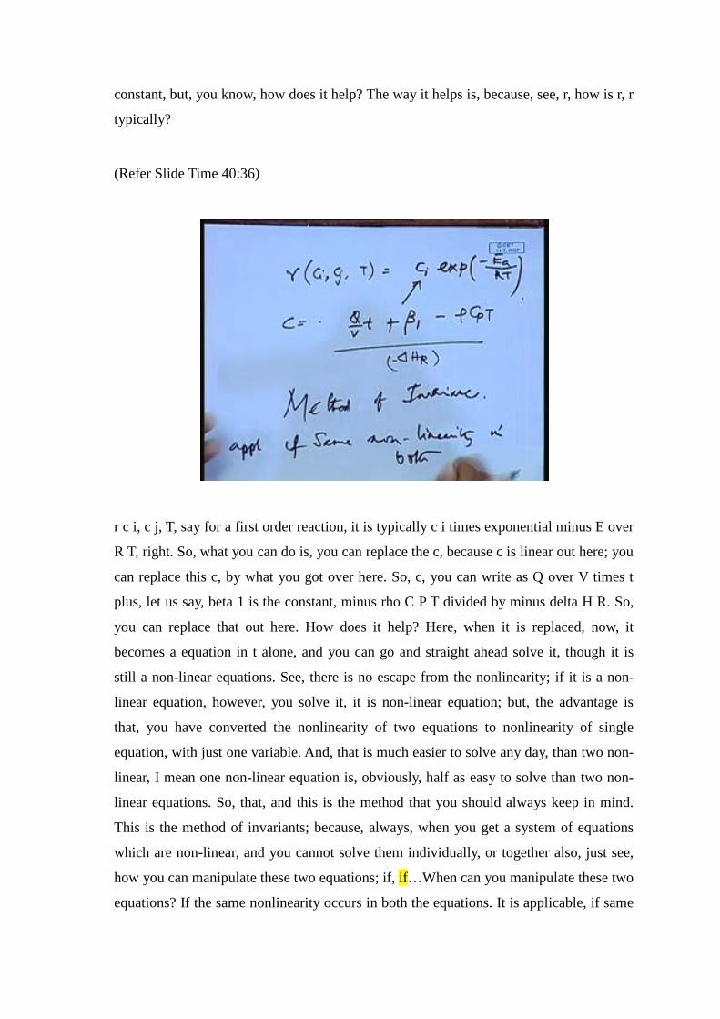
r c i, c j, T, say for a first order reaction, it is typically c i times exponential minus E over

R T, right. So, what you can do is, you can replace the c, because c is linear out here; you

can replace this c, by what you got over here. So, c, you can write as Q over V times t

plus, let us say, beta 1 is the constant, minus rho C P T divided by minus delta H R. So,

you can replace that out here. How does it help? Here, when it is replaced, now, it

becomes a equation in t alone, and you can go and straight ahead solve it, though it is

still a non-linear equations. See, there is no escape from the nonlinearity; if it is a non-

linear equation, however, you solve it, it is non-linear equation; but, the advantage is

that, you have converted the nonlinearity of two equations to nonlinearity of single

equation, with just one variable. And, that is much easier to solve any day, than two non-

linear, I mean one non-linear equation is, obviously, half as easy to solve than two non-

linear equations. So, that, and this is the method that you should always keep in mind.

This is the method of invariants; because, always, when you get a system of equations

which are non-linear, and you cannot solve them individually, or together also, just see,

how you can manipulate these two equations; if, if…When can you manipulate these two

equations? If the same nonlinearity occurs in both the equations. It is applicable, if same

nonlinearity in both, fine. So, why I am saying all this is because, we are going to do, use

some of these in the latter part of the course.


So, so, anyhow. So, using the method of invariants, this is what we got. We just did the,

did the calculation, I think, we have it out here; let us see here. So, here, on the page, if

you see. So, we, we did this and the initial conditions are, X equals X 0 at t equal 0, S

equals S 0. Now, this we have converted into a equation in S alone and we can integrate

this, as we, as we said. So, this is the invariants and we walked through all of this.


So, I think, I can just skip that, right. So, on integration, this is what you get. This is, this

is the whole thing that you got, and how do you get this? Using, as I said, just using

partial fractions, from this side, you know, just take it to the denominator, use the partial

fractions; then, you will get exponential for both cases, and this is the solution you got.

So, here X 0 is the cell concentration at time t equals 0 and S 0 is the substrate

concentration at time t equals 0. There is a (( )) here, you know, and what is that? The ((

)) is that, look at the, look at the equation; if X 0 is 0, then, this solution does not hold.

So, you have to go back and resolve it, because X 0 is most typically, might be 0; you

know, not, not most typically, but, might be 0; there might be cases, when you take a

feed, which has no cell, I mean, not all times; but, there could be times, when you take a

feed which has no cells at all, or very negligible concentration of cell, then, this will

blow up. So, you just need to go back and put that, so, into the equation, and then solve

it, rather than solve it and put it into the solutions.

So, if the product that is formed, is formed from a culture, that is, from the, you know,

growth model that we gave, and there are some other sources of cell formation apart

from the culture, then, what will you do? It is straightforward, you know. What is the

growth model? The growth model is d x d t equals mu X. So, what you will do in that

case is, just use that d x d t equals mu X plus beta X, where beta is from non-cultured

sources. So, unlike mu, which is the function of S, substrate, beta is not going to be a

function of S. It is simply going to be a constant, but, you will have a non-cultured

sources, then you could use something like this. So, del P del t, the product formation

would be, some alpha times mu times S X over X plus K plus S, that is the Monod plus

model, plus beta X, and beta being a constant. And, how do you think, this will affect the

product formation? It will, obviously, increase, but, in which way? In, in qualitatively

which way it will increase? Obviously, it will increase, not to say that.

(( ))

Yes, slope will definitely change, but, what would, more than that change, is the

saturation. Because, see, this, it reaches a level of saturation. Because, in the Monod

growth model, there is a level of saturation; but, in this, the level of saturation would

change. So, this is how it looks like, see. So, the product that you get…So, this is the

product by the way, you know. So, slightly different from the cell; so, the cells are, you

know, cell culture you are doing, and because of the cells, a product is being formed; I

mean, I probably did not explain it, probably. So, this is the, we, this is different from

what we did before. So, the cell, cell is being produced X, but, because of the cell, a

product is being formed, which is, which is slope beta.


So, and the substrate is here, just like before, because the substrate is being consumed

only in the cell formation. So, exactly the same, same way as before; the negative of

Monod growth kinetics, as you can see, you know, just, just the thing flipped around,

because, whatever is taken, the substrate is being taken up, consumed and not formed.

So, it is exactly the Monod growth kinetics flipped around. The cells, again, you see,

there is a Monod growth kinetics, the formation of the cell; but, the product formation is

not going to saturate out as I said, because, there is a term, which is the, which is the

constant and it goes, linearly increases, fine.

(( ))

It does not have to be linear, because, it depends on the product formation; but, it could

be, it could even be beta x square, you know atmost; but, I, it is not going to be

exponential of something. It does not have to be linear. See, big what is essentially

happening, what we are trying to say over here, the cells are formed and the cells leads to

some other products. Now, what that, could that reaction be? That could be a first order

reaction; that could be a second order reaction; it can be third order reaction, or any

higher order. It cannot be an exponential dependent. What, one possibility is that, the

exponential depence on temperature; that, that is the possibility.


So, beta, for example, beta X could be such that, some beta 0 exponential minus E a over

R T times X. So, that is the possibility. So, that is one possibility, or you can have, you

know; or, beta itself could be, it could go as beta 1 or beta 0 times X, so, which, in which

case, it could be a second order. So, anyhow. So, all we are trying to say is that, the

products that are formed, you know, it, it is not going to saturate out; whereas the cell

formation could saturate out and the substrate formation, substrate consumption could go

on, and it can go reach 0, the substrate concentration; but the product formation will go,

ok.

So, I think, the next thing that we will start is with, we do not have a lot of time today,

but, just to give you a brief overview, is a concept of death of cells. We have been

looking at the growth of cells, but, what happens when there is a death of cells, and the

answer is…Would any of you want to tell me? It is very similar to what we did just now.

(( ))

Yes. So, this just could be minus beta kind of thing. So, if you remember, do you

remember that, we did the microbial growth models and we talked about, I think, I have

the slide with me, and I can even go in there; let us see; yes, here. So, here, you know we

talked about the, yes, you remember this, right.


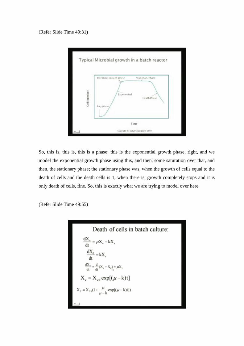
So, this is, this is, this is a phase; this is the exponential growth phase, right, and we

model the exponential growth phase using this, and then, some saturation over that, and

then, the stationary phase; the stationary phase was, when the growth of cells equal to the

death of cells and the death cells is 1, when there is, growth completely stops and it is

only death of cells, fine. So, this is exactly what we are trying to model over here.


So, this is the growth. So, the stationary phase and the death phase. So, that is what we

are trying to model over here now. So, d x d t equals mu X minus k X. Why do I put the

v? v is for some live cells, just for live cells. So, k is going to be, remember, k is going to

be a constant; k is not dependent on the substrate, whereas mu is dependent on the

substrates. d x d x d t d t equals k v, d d v, dead cells, right. And, I went on and talked

about the whole experiment, if you remember, of doing another microscope and

checking, how to check the number of dead cells, do you remember all that? So, this is,

this is the very natural corollary of the entire incubation process and there is no running

away from the fact that, there are always going to be a lot of dead cells, when you deal

with them. So, again, you see that, we, we do some kind of invariants out here. We say

the total number of cells that you have in the system, like we did in the last class, is not a

constant, but, it is increasing with time, or decreasing with time, whatever is this, is that,

and that is mu times X v, fine

So, X v is X v 0 times exponential mu minus k times t, right, from the first equation;

very straightforward; and, X T is this. How do you get this? So, you just solve for X v,

put it up into this equation, and then, you can directly solve for X T. So, this is what we

get here. So, this, this number, you know, it depends, now. Now, what does it depend on?

Like, you see, whether this is going to be a stationary phase, or whether it is going to be

a decay, so, how, how do you define that? When mu is very close to k, for example, it is

more or less in the stationary phase; because, this term is kind of 0, and you know, this,

this term is close to 1, so, it will be a constant. When mu is less than k, then, it starts to

decay in the death phase. So, typically, in the first part of it, the mu is much larger than k.

So, it keeps increasing, and then, mu is, when it is close to k, then, it is in the stationary

phase; and then, when it goes to decay...So, here is plot for that, yes. So, here, here is,

here is the plot. So, in this, this, in this phase, mu is greater than k, much, much greater

than k; in this phase, mu is more or less close to k. So, as a result, there is more or less

constant and this phase, mu is much less than k.

So, I think, we will stop. There is some something else in the next slide is yes, next slide

we go into the ideal C S T R models. I think, we will stop here with the death of cells

and that concludes everything to do with the batch reactor model. And next class, we will

start the chemostat, but, I will try to, I will remember to bring the years, and the

references for the history, because, that is a pretty interesting thing, I think. So, is there

any questions before we conclude, in today's lecture? Then, we will stop here today and

we will continue with the C S T R in the next lecture.

Date post:	19-Jul-2018
Category:	Documents
Upload:	duongdat
View:	212 times
Download:	0 times

Biochemical Engineering Prof. Dr. Rintu Banerjee ...textofvideo.nptel.ac.in/103105054/lec26.pdf ·...

Documents