Biochemical Pathway Robustness Prediction with Graph Neural Networks Marco Podda 1 , Davide Bacciu 1 , Alessio Micheli 1 , Paolo Milazzo 1 * 1 University of Pisa - Department of Computer Science Largo Bruno Pontecorvo 3, 56127, Pisa - Italy Abstract. The robustness property of a biochemical pathway refers to maintaining stable levels of molecular concentration against the per- turbation of parameters governing the underlying chemical reactions. Its computation requires an expensive integration in parameter space. We present a novel application of Graph Neural Networks (GNN) to predict robustness indicators on pathways represented as Petri nets, without the need of performing costly simulations. Our assumption is that pathway structure alone is sufficient to be effective in this task. We show experi- mentally for the first time that this is indeed possible to a good extent, and investigate how different architectural choices influence performances. 1 Introduction Biological pathways describe the complex interactions between molecules at the biochemical level. Pathways are usually represented as graphs, while Ordinary Differential Equations (ODEs) are often used to investigate their dynamical properties. Among them, robustness [1] is one of particular relevance. It can be defined on a pair of input and output molecules, and it quantifies the stability of the steady-state concentration of the output against perturbations in the initial concentration of the input (α-robustness, [2]). To assess robustness, the graph representation of the pathway must be translated into a set of ODEs. Then, the property is calculated via integration in parameter space, which requires a massive amount of computational resources. We present a novel and challenging application of Graph Neural Networks (GNNs) [3, 4] in the field of computational biology. Specifically, we introduce the use of GNNs for pathway robustness pre- diction. The assumption underlying this study is that the structure of a pathway contains sufficient information to predict robustness indicators without having to perform expensive numerical simulations. To test this assumption, we apply GNNs to a dataset of pathways graphically represented as Petri nets [5]. We perform an extensive evaluation of six GNN variants on the task, studying how the number of layers affects performances. Our experiments show that GNNs are indeed capable of predicting robustness to a good extent. These preliminary results can ultimately lead to faster advances in the field: in particular, this approach could relieve researchers from the need of performing expensive simu- lations in order to evaluate not only robustness, but also dynamical properties such as bistability, monotonicity and oscillations. * This work has been partially supported by the Italian Ministry of Education, University, and Research (MIUR) under project SIR 2014 LIST-IT (grant n. RBSI14STDE). ESANN 2020 proceedings, European Symposium on Artificial Neural Networks, Computational Intelligence and Machine Learning. Online event, 2-4 October 2020, i6doc.com publ., ISBN 978-2-87587-074-2. Available from http://www.i6doc.com/en/. 121
Marco Podda1, Davide Bacciu1, Alessio Micheli1, Paolo Milazzo1 ∗
1 University of Pisa - Department of Computer ScienceLargo Bruno Pontecorvo 3, 56127, Pisa - Italy
Abstract. The robustness property of a biochemical pathway refersto maintaining stable levels of molecular concentration against the per-turbation of parameters governing the underlying chemical reactions. Itscomputation requires an expensive integration in parameter space. Wepresent a novel application of Graph Neural Networks (GNN) to predictrobustness indicators on pathways represented as Petri nets, without theneed of performing costly simulations. Our assumption is that pathwaystructure alone is sufficient to be effective in this task. We show experi-mentally for the first time that this is indeed possible to a good extent,and investigate how different architectural choices influence performances.
1 Introduction
Biological pathways describe the complex interactions between molecules at thebiochemical level. Pathways are usually represented as graphs, while OrdinaryDifferential Equations (ODEs) are often used to investigate their dynamicalproperties. Among them, robustness [1] is one of particular relevance. It can bedefined on a pair of input and output molecules, and it quantifies the stability ofthe steady-state concentration of the output against perturbations in the initialconcentration of the input (α-robustness, [2]). To assess robustness, the graphrepresentation of the pathway must be translated into a set of ODEs. Then,the property is calculated via integration in parameter space, which requires amassive amount of computational resources. We present a novel and challengingapplication of Graph Neural Networks (GNNs) [3, 4] in the field of computationalbiology. Specifically, we introduce the use of GNNs for pathway robustness pre-diction. The assumption underlying this study is that the structure of a pathwaycontains sufficient information to predict robustness indicators without havingto perform expensive numerical simulations. To test this assumption, we applyGNNs to a dataset of pathways graphically represented as Petri nets [5]. Weperform an extensive evaluation of six GNN variants on the task, studying howthe number of layers affects performances. Our experiments show that GNNsare indeed capable of predicting robustness to a good extent. These preliminaryresults can ultimately lead to faster advances in the field: in particular, thisapproach could relieve researchers from the need of performing expensive simu-lations in order to evaluate not only robustness, but also dynamical propertiessuch as bistability, monotonicity and oscillations.
∗This work has been partially supported by the Italian Ministry of Education, University,and Research (MIUR) under project SIR 2014 LIST-IT (grant n. RBSI14STDE).
ESANN 2020 proceedings, European Symposium on Artificial Neural Networks, Computational Intelligence and Machine Learning. Online event, 2-4 October 2020, i6doc.com publ., ISBN 978-2-87587-074-2. Available from http://www.i6doc.com/en/.
Fig. 1: a) A set of chemical reactions in arrow notation, with promot-ers/inhibitors above the arrows. b) The associated ODE system (example). c)The Pathway Petri net corresponding to the chemical reactions. d) An exampleof training graph: circle nodes are molecules, box nodes are reactions. Differentedge styles identify the three possible relations (standard, promoter, inhibitor).
2 Background and Notation
A chemical reaction is a process that transforms a group of molecules (reactants)into another (products). Reactions are governed by kinetic constants, that spec-ify the rate at which the reaction can occur, given the concentrations of thereactants in a chemical solution. In reactions, molecules can also play the rolespromoters (reaction facilitators) or inhibitors (reaction blockers). A biochemicalpathway is a system of related chemical reactions, where the product of one maybecome the reactant of another. Petri nets are a common modeling notationfor pathways. We consider here a variant of Petri nets that suitably considerspromoters and inhibitors, that we call Pathway Petri nets (PPNs). The seman-tics of a PPN is described by an ODE system that models the associated set ofreactions. The state of a PPN (called marking) corresponds to an assignment ofpositive real values to the variables associated to the system. Given M , the setof possible markings, a PPN is defined as a tuple P = (P, T, f, p, h, δ,m0) where:
• P and T are finite, non empty, disjoint sets of places and transitions;
• f : ((P ×T )∪ (T ×P ))→ N≥0 defines the set of directed arcs, weighted bynon-negative integers (whose value corresponds to the multiplicity of thereactants/products in the reaction);
• p, h ⊆ (P × T ) are the sets of promotion and inhibition arcs;
• δ : T → Ψ, with Ψ = M → R≥0, is a function that assigns to eachtransition a function corresponding to the computation of a kinetic formulato every possible marking m ∈M ;
• m0 ∈M is the initial marking.
Given a PPN P, we can cast it into a graph GP = 〈V,E〉 as follows. Firstwe define the node sets Vmol for molecules, and Vreact for reactions, and set
ESANN 2020 proceedings, European Symposium on Artificial Neural Networks, Computational Intelligence and Machine Learning. Online event, 2-4 October 2020, i6doc.com publ., ISBN 978-2-87587-074-2. Available from http://www.i6doc.com/en/.
122
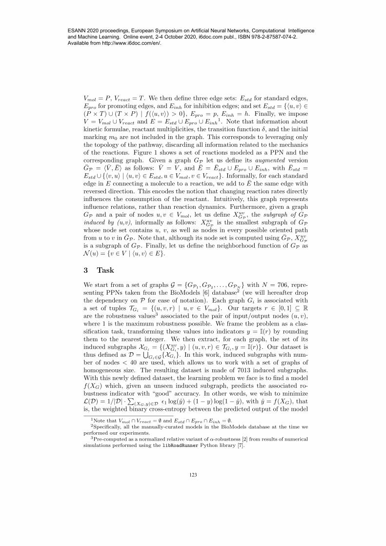
Vmol = P , Vreact = T . We then define three edge sets: Estd for standard edges,Epro for promoting edges, and Einh for inhibition edges; and set Estd = {〈u, v〉 ∈(P × T ) ∪ (T × P ) | f(〈u, v〉) > 0}, Epro = p, Einh = h. Finally, we imposeV = Vmol ∪ Vreact and E = Estd ∪ Epro ∪ Einh
1. Note that information aboutkinetic formulae, reactant multiplicities, the transition function δ, and the initialmarking m0 are not included in the graph. This corresponds to leveraging onlythe topology of the pathway, discarding all information related to the mechanicsof the reactions. Figure 1 shows a set of reactions modeled as a PPN and thecorresponding graph. Given a graph GP let us define its augmented versionGP = 〈V , E〉 as follows: V = V , and E = Estd ∪ Epro ∪ Einh, with Estd =Estd ∪{〈v, u〉 | 〈u, v〉 ∈ Estd, u ∈ Vmol, v ∈ Vreact}. Informally, for each standardedge in E connecting a molecule to a reaction, we add to E the same edge withreversed direction. This encodes the notion that changing reaction rates directlyinfluences the consumption of the reactant. Intuitively, this graph representsinfluence relations, rather than reaction dynamics. Furthermore, given a graphGP and a pair of nodes u, v ∈ Vmol, let us define Xuv
GP, the subgraph of GP
induced by (u,v), informally as follows: XuvGP
is the smallest subgraph of GPwhose node set contains u, v, as well as nodes in every possible oriented pathfrom u to v in GP . Note that, although its node set is computed using GP , Xuv
GPis a subgraph of GP . Finally, let us define the neighborhood function of GP asN (u) = {v ∈ V | 〈u, v〉 ∈ E}.
3 Task
We start from a set of graphs G = {GP1, GP2
, . . . , GPN} with N = 706, repre-
senting PPNs taken from the BioModels [6] database2 (we will hereafter dropthe dependency on P for ease of notation). Each graph Gi is associated witha set of tuples TGi = {(u, v, r) | u, v ∈ Vmol}. Our targets r ∈ [0, 1] ⊆ Rare the robustness values3 associated to the pair of input/output nodes (u, v),where 1 is the maximum robustness possible. We frame the problem as a clas-sification task, transforming these values into indicators y = I(r) by roundingthem to the nearest integer. We then extract, for each graph, the set of itsinduced subgraphs XGi
= {(XuvGi, y) | (u, v, r) ∈ TGi
, y = I(r)}. Our dataset isthus defined as D =
⋃Gi∈G{XGi}. In this work, induced subgraphs with num-
ber of nodes < 40 are used, which allows us to work with a set of graphs ofhomogeneous size. The resulting dataset is made of 7013 induced subgraphs.With this newly defined dataset, the learning problem we face is to find a modelf(XG) which, given an unseen induced subgraph, predicts the associated ro-bustness indicator with “good” accuracy. In other words, we wish to minimizeL(D) = 1/|D| ·
∑(XG,y)∈D ε1 log(y) + (1 − y) log(1 − y), with y = f(XG), that
is, the weighted binary cross-entropy between the predicted output of the model
1Note that Vmol ∩ Vreact = ∅ and Estd ∩ Epro ∩ Einh = ∅.2Specifically, all the manually-curated models in the BioModels database at the time we
performed our experiments.3Pre-computed as a normalized relative variant of α-robustness [2] from results of numerical
simulations performed using the libRoadRunner Python library [7].
ESANN 2020 proceedings, European Symposium on Artificial Neural Networks, Computational Intelligence and Machine Learning. Online event, 2-4 October 2020, i6doc.com publ., ISBN 978-2-87587-074-2. Available from http://www.i6doc.com/en/.
123
y and the actual indicator y. Weighting with ε1 = #negative examples#positive examples is needed to
mitigate the imbalance in favor of the positive class (72%-28%).
4 Model
Our model uses GNNs to embed the structure of subgraphs XG. GNNs are basedon the notion of state, a vector associated to each node in the graph which isupdated iteratively according to a message-passing schema [8]. The initial stateis set to be a vector of features: in our case, each subgraph node contains abinary feature vector of size 3, where the first position encodes node type (0 formolecule, 1 for reaction); the second position encodes whether a node is an inputnode (1) or not (0); the third position encodes whether a node is a output node(1) or not (0). In general, the `-th layer of a GNN updates the state of a nodev as h`+1
v = σ(w` U(h`v, C({h`+1
u | u ∈ N (v)})), where C is a function thataggregates nodes in the neighborhood of the current node; U is an update func-tion that combines hv, the current state of the node with the aggregated stateof its neighbors; w` are adaptive weights; and σ is a nonlinearity (ReLU in ourcase). To build a graph-level representation at layer `, node representations areaggregated by a permutation-invariant readout function h` = R({h`
v | v ∈ V }).Note that different GNNs can be derived choosing different C, U , and R. Thefinal representation of the graph is obtained concatenating the representations ofeach layer; more formally, hG = [h1;h2; . . . ;hL], where ; denotes concatenation,and L is the number of GNN layers. We denote the process of obtaining thefinal graph representation as hG = GNN(XG). The graph representation is thenfed to a Multi-Layer Perceptron (MLP) classifier with two hidden layers withReLU activations, and sigmoid outputs that compute the robustness probabilityassociated to the input subgraph. Summing up, our model f is implemented asthe following neural network: f(XG) = MLP(GNN(XG)), where we omit theparameterization for ease of notation.
5 Experiments
We thoroughly assess the performance of the model described in Section 4 usingnested Cross-Validation (CV) [9] for generalization accuracy estimation, with anouter 5-fold CV for performance assessment and an internal holdout split (90%training, 10% validation) for model selection. The model is selected with gridsearch on the following hyper-parameters: size of the GNN embedding (choosingbetween 64 and 128 per layer), number of GNN layers (choosing from {1, . . . , 8}),and type of readout function (choosing among element-wise mean, max or sum).We evaluate 6 different models, determined by the type of convolution adoptedand whether or not edge features are learned. Specifically, we evaluate threedifferent convolutions: Graph Convolutional Network (GCN) [10], Graph Iso-morphism Network (GIN) [11] and Weisfeiler-Lehman GCN (WLGCN) [12]. Foreach of them, we evaluate a vanilla variant which uses the state update functiondescribed in Section 4, as well as an edge-aware variant (following [13]) where
ESANN 2020 proceedings, European Symposium on Artificial Neural Networks, Computational Intelligence and Machine Learning. Online event, 2-4 October 2020, i6doc.com publ., ISBN 978-2-87587-074-2. Available from http://www.i6doc.com/en/.
124
each edge type has its own set of adaptive weights. Formally, the edge-aware vari-ants update the state as h`+1
v = σ(∑
k∈K w`k U(h`
v, C({h`+1u | u ∈ N (v, k)})),
where k ranges over all K possible edge types, and N (v, k) is a neighborhoodfunction that only selects neighbors of v connected by an edge of type k. Allmodels are trained with the Adam optimizer, using a learning rate of 0.001 andscheduled annealing with a shrinking factor of 0.6 every 50 epochs. The sizeof the two hidden layers of the MLP is 128 and 64, with dropout rate of 0.1.All models are trained for a total of 500 epochs; we use early stopping on thevalidation accuracy with 100 epochs of patience. In the assessment phase, themodel is trained three different times to account for random initialization effects;the resulting accuracies are averaged to obtain the final test fold accuracy. Theexperiments are implemented using the PyTorch Geometrics library [14].
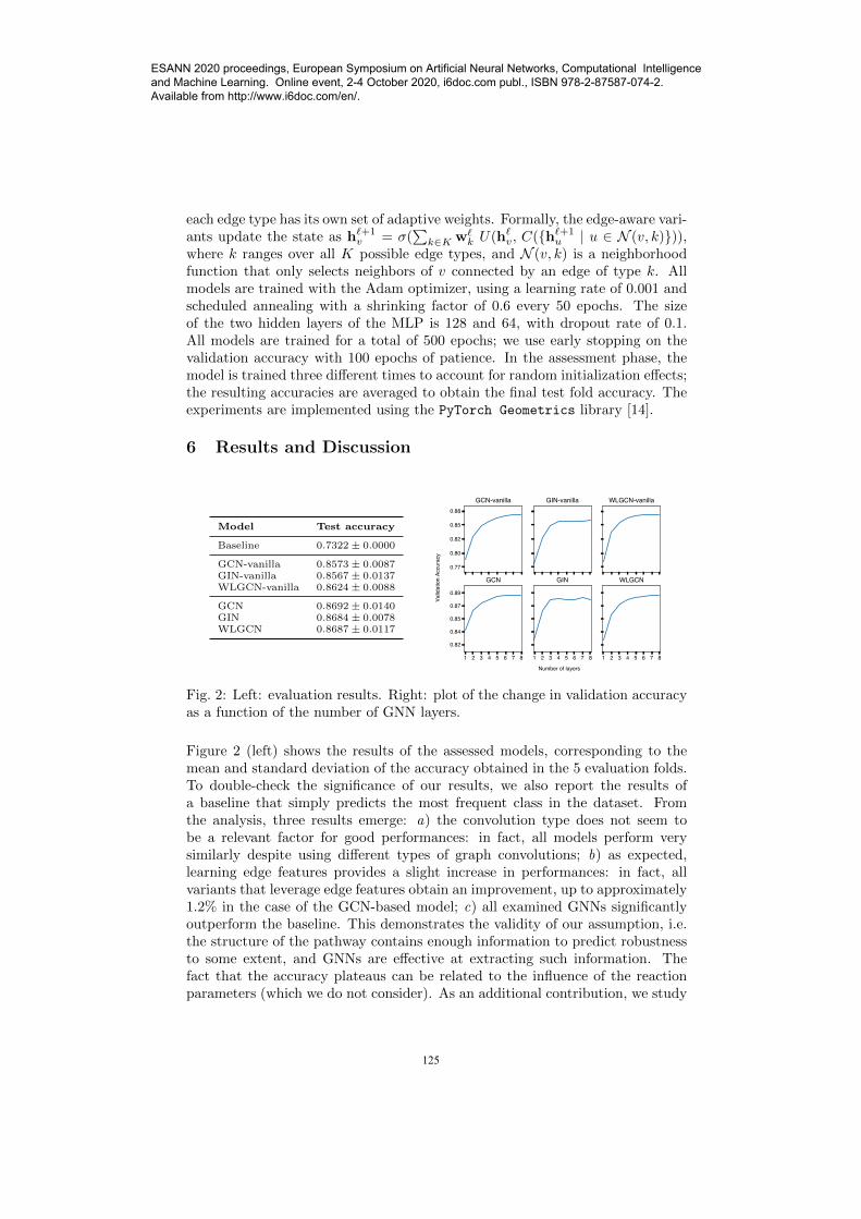
Fig. 2: Left: evaluation results. Right: plot of the change in validation accuracyas a function of the number of GNN layers.
Figure 2 (left) shows the results of the assessed models, corresponding to themean and standard deviation of the accuracy obtained in the 5 evaluation folds.To double-check the significance of our results, we also report the results ofa baseline that simply predicts the most frequent class in the dataset. Fromthe analysis, three results emerge: a) the convolution type does not seem tobe a relevant factor for good performances: in fact, all models perform verysimilarly despite using different types of graph convolutions; b) as expected,learning edge features provides a slight increase in performances: in fact, allvariants that leverage edge features obtain an improvement, up to approximately1.2% in the case of the GCN-based model; c) all examined GNNs significantlyoutperform the baseline. This demonstrates the validity of our assumption, i.e.the structure of the pathway contains enough information to predict robustnessto some extent, and GNNs are effective at extracting such information. Thefact that the accuracy plateaus can be related to the influence of the reactionparameters (which we do not consider). As an additional contribution, we study
ESANN 2020 proceedings, European Symposium on Artificial Neural Networks, Computational Intelligence and Machine Learning. Online event, 2-4 October 2020, i6doc.com publ., ISBN 978-2-87587-074-2. Available from http://www.i6doc.com/en/.
125
how GNN layering affects performances. To do so, we perform an ablation studywhere we stratify the results of the model selection by number of GNN layers,and report the mean and standard deviations of the related validation accuracies.Note that, although validation accuracy is in general an over-estimate of the trueaccuracy, the relative difference in performance as the number of layers changestays proportional independently of the data used. Figure 2 (right) shows that,for all considered GNNs, increasing the number of layers improves accuracy, upto a certain depth where it becomes stable. This provides evidence that “deep”GNNs are necessary to obtain good performances in this task.
7 Conclusions
In this work we have shown, for the first time, that GNNs can be effective atpredicting the dynamical property of robustness of pathway networks, leveragingonly their structure. Future works will be aimed to extend this result to largergraphs as well as to other interesting dynamical properties.
References
[1] H. Kitano. Biological robustness. Nature Reviews Genetics, 5(11):826, 2004.
[2] L. Nasti, R. Gori, and P. Milazzo. Formalizing a notion of concentration robustnessfor biochemical networks. In STAF Workshops, volume 11176 of LNCS, pages 81–97.Springer, 2018.
[3] F. Scarselli, M. Gori, et al. The Graph Neural Network Model. Trans. Neur. Netw.,20(1):61–80, 2009.
[4] A. Micheli. Neural Network for Graphs: A Contextual Constructive Approach. Trans.Neur. Netw., 20(3):498–511, 2009.
[5] V. N. Reddy, M. L. Mavrovouniotis, et al. Petri net representations in metabolic pathways.In ISMB, volume 93, pages 328–336, 1993.
[6] C. Li, M. Donizelli, et al. BioModels Database: An enhanced, curated and annotatedresource for published quantitative kinetic models. BMC Systems Biology, 4:92, 2010.
[7] E. T. Somogyi, J. M. Bouteiller, et al. libRoadRunner: a high performance SBML simu-lation and analysis library. Bioinformatics, 31(20):3315–3321, 2015.
[8] J. Gilmer, S. S. Schoenholz, et al. Neural message passing for quantum chemistry. InInternational Conference on Machine Learning, 2017.
[9] S. Varma and R. Simon. Bias in Error Estimation When Using Cross-Validation for ModelSelection. BMC bioinformatics, 7:91, 2006.
[10] T. N. Kipf and M. Welling. Semi-Supervised Classification with Graph ConvolutionalNetworks. In International Conference on Learning Representations, 2017.
[11] K. Xu, W. Hu, et al. How Powerful are Graph Neural Networks? In InternationalConference on Learning Representations, 2019.
[12] C. Morris, M. Ritzert, et al. Weisfeiler and Leman Go Neural: Higher-Order GraphNeural Networks. In Proceedings of the 33rd Conference on Artificial Intelligence, AAAI’19, pages 4602–4609, 2019.
[13] M. S. Schlichtkrull, T. N. Kipf, et al. Modeling Relational Data with Graph ConvolutionalNetworks. In Proceedings of the 15th International Conference on The Semantic Web,ESWC ’18, pages 593–607, 2018.
[14] M. Fey and J. E. Lenssen. Fast Graph Representation Learning with PyTorch Geometric.In ICLR Workshop on Representation Learning on Graphs and Manifolds, 2019.
ESANN 2020 proceedings, European Symposium on Artificial Neural Networks, Computational Intelligence and Machine Learning. Online event, 2-4 October 2020, i6doc.com publ., ISBN 978-2-87587-074-2. Available from http://www.i6doc.com/en/.


![Equilibrium distributions of simple biochemical reaction ...hespanha/published/20140054-full.pdfthe bacteriophage l lysis–lysogeny pathway [1]), or other methods (e.g. balanced truncation,](https://static.documents.pub/doc/80x56/5f49035e1111604a19761499/equilibrium-distributions-of-simple-biochemical-reaction-hespanhapublished20140054-fullpdf.jpg)


