This is a reformatted version of an article that appeared in Rev. Modern Physics 66, 1481-1507 (1994)

Biological Pattern Formation : from Basic Mechanisms to ComplexStructures

A. J. Koch1 and H. MeinhardtMax Planck Institute for Developmental Biology

Spemannstr. 35, D- 72076 Tubingenhttp://www.eb.tuebingen.mpg.de/meinhardt; hans.meinhardt@tuebingen.mpg.de

The reliable development of highly complex organ-isms is an intriguing and fascinating problem. Thegenetic material is, as a rule, the same in each cellof an organism. How do then cells, under the influ-ence of their common genes, produce spatial pat-terns ? Simple models are discussed that describethe generation of patterns out of an initially nearlyhomogeneous state. They are based on nonlinearinteractions of at least two chemicals and on theirdiffusion. The concepts of local autocatalysis and oflong range inhibition play a fundamental role. Nu-merical simulations show that the models accountfor many basic biological observations such as theregeneration of a pattern after excision of tissue orthe production of regular (or nearly regular) arrays oforgans during production of regular (or nearly regu-lar) arrays of organs during (or after) completion ofgrowth.Very complex patterns can be generated in a repro-ducible way by hierarchical coupling of several suchelementary reactions. Applications to animal coatingand to the generation of polygonally shaped patternsare provided. It is further shown how to generate astrictly periodic pattern of units that themselves ex-hibit a complex and polar fine structure. This is il-lustrated by two examples : the assembly of photore-ceptor cells in the eye of Drosophila and the position-ing of leaves and axillary buds in a growing shoot. Inboth cases, the substructures have to achieve an in-ternal polarity under the influence of some primarypattern forming system existing in the fly’s eye or inthe plant. The fact that similar models can describeessential steps in so distantly related organisms asanimals and plants suggests that they reveal someuniversal mechanisms.

1. INTRODUCTIONA most fascinating aspect of biological systems is thegeneration of complex organisms in each round of thelife cycle. Higher organisms develop, as the rule, from asingle fertilized egg. The result is a highly reproduciblearrangement of differentiated cells. Many processes areinvolved, for example cell differentiation, cell movement,shape changes of cells and tissues, region-specific con-trol of cell division and cell death. Development of anorganism is, of course, under genetic control but the ge-netic information is usually the same in all cells. A crucialproblem is therefore the generation of spatial patternsthat allow a different fate of some cells in relation to oth-ers.

The complexity of the evolving pattern seems to pre-clude any mathematical theory. However, by experi-mental interference with a developing organism it hasturned out that the individual steps are fairly indepen-dent of each other. For instance, the organization of theanteroposterior axis (i.e., the head to tail pattern) in aDrosophila embryo is controlled by a completely differentset of genes than the dorsoventral axis. Shortly after itsinitiation, the development of a wing is largely indepen-dent of the surrounding tissue and can progress even atan ectopic position after transplantation. Therefore, mod-els can be written for elementary steps in development.The linkage of these steps requires then a second ap-proximation.

The necessity of mathematical models for morpho-genesis is evident. Pattern formation is certainly basedon the interaction of many components. Since the inter-actions are expected to be nonlinear, our intuition is in-sufficient to check whether a particular assumption reallyaccounts for the experimental observation. By modelling,the weak points of an hypothesis become evident and theinitial hypothesis can be modified or improved. Modelscontain often simplifying assumptions and different mod-els may account equally well for a particular observation.This diversity should however be considered as an ad-vantage : multiplicity of models stimulates the design of

1

experimental tests in order to discriminate between therival theories. In this way, theoretical considerations pro-vide substantial help to the understanding of the mecha-nisms on which development is based (Berking, 1981).

In his pioneering work, Turing (1952) has shown thatunder certain conditions two interacting chemicals cangenerate a stable inhomogeneous pattern if one of thesubstances diffuses much faster than the other. Thisresult goes against “common sense” since diffusion isexpected to smooth out concentration differences ratherthan to generate them.

However, Turing apologizes for the strange and un-likely chemical reaction he used in his study. Meanwhile,biochemically more feasible models have been devel-oped and applied to different developmental situations(Lefever, 1968 ; Gierer and Meinhardt, 1972 ; Gierer,1977 ; Murray, 1990). Chemical systems have alsobeen intensively investigated for their ability to produce“Turing patterns” : some experiments present beautifulreaction-diffusion structures in open reactors (Ouyang etal., 1989 ; Castets et al, 1990 ; de Kepper et al., 1991).

In the first part of this article, after having shortly dis-cussed the relevance of chemical gradients in biologicalsystems, we shall present simple models of pattern for-mation and their common basis, local self-enhancementand long range inhibition. The patterns that can begenerated are graded concentration profiles, local con-centration maxima and stripe-like distributions of sub-stances. In the second part we shall show how morecomplex patterns can be generated by hierarchical su-perimposition of several pattern forming systems. Theformation of a regular periodic arrangement of differentcell types or the generation of polygonal patterns will bediscussed. The models of that section are original andso far unpublished.

Appendix 7 contains a complete discussion of the lin-ear stability analysis in the case of the simplest models.The parameters used for the simulations presented here-after are listed in Appendix 8. A reader interested in nu-merical simulations should feel no difficulty to reproduceor improve the results.

Throughout the paper, comparisons of models withexperimental observations are provided. If necessary thebiological background is outlined in such a way that thearticle should be understandable without previous knowl-edge of biology.

2. GRADIENTS IN BIOLOGICAL SYSTEMSIn many developmental systems small regions play animportant role because they are able to organize the fateof the surrounding tissue. The mouth opening of a hy-dra or the dorsal lip of an amphibian blastula are wellknown examples. Transplantation of a small piece ofsuch an organizing centre into an ectopic position canchange the fate of the surrounding tissue : these cells arethen instructed to form those structures that are induced

in the normal neighborhood of such an organizing re-gion. Based on these observations, Wolpert (1969) hasworked out the concept of positional information. The lo-cal concentration of a substance that is distributed in agraded fashion dictates the direction in which a group ofcells has to develop. The organizing region is thoughtto be the source of such a morphogenetic substance. Afamous example is the determination of the digits in thechick wing bud (Cooke and Summerbell, 1980 ; Tickle,1981). It occurs under control of a small nest of cells lo-cated at the posterior border of the wing bud, the zoneof polarizing activity (ZPA). The results nicely fit withthe assumption of some hypothetical substance diffus-ing out of the ZPA and producing a concentration gradi-ent ; groups of cells form the correct digit by measuringthe local concentration within this gradient (Summerbell,1974 ; Wolpert and Hornbruch, 1981). Many experimentsin which a second ZPA is implanted at various positionsof the wing bud confirm this conjecture : supernumer-ary digits are then formed at abnormal positions but inaccordance with the pattern predicted by the assumedgradient produced by the two ZPA. A possible candidatefor the morphogenetic substance is retinoic acid (Thallerand Eichele, 1987, 1988). Indeed, small beets soakedwith this substance at low concentrations mimic all theeffects of a ZPA.

Nowadays there is a growing body of evidence thatchemical gradients play a key role in pattern formationand cell differentiation. For instance, it has been ob-served that the protein bicoid has a graded concentra-tion distribution in the Drosophila melanogaster embryo ;it organizes the anterior half of the fly and has been fullycharacterized (Driever and Nusslein-Volhard, 1988 ; Bor-ing et al., 1993).

In this context, theoretical models have to give satis-factory answers to the following two questions.

• How can a system give rise and maintain largescale inhomogeneities like gradients even whenstarting from initially more or less homogeneousconditions ?

• How do cells measure the local concentration inorder to interpret their position in a gradient andchoose the corresponding developmental path-way ?

The next two sections are devoted to the first question.We shall discuss theoretical models having the abilityto produce graded distributions of chemical substancesand present their regulation characteristics. In the sub-sequent section, we shall show how to use the positionalinformation contained in gradients in order to induce acorrect differentiation.

2

3. SIMPLE MODELS FOR PATTERNFORMATION

As mentioned, Turing (1952), was the first who realizedthat the interaction of two substances with different dif-fusion rates can cause pattern formation. Gierer andMeinhardt (1972) and independently Segel and Jackson(1972) have shown that two features play a central role :local self-enhancement and long range inhibition. It isessential to have an intuitive understanding of these tworequirements since they lay at the heart of pattern forma-tion.

Self-enhancement is essential for small local inhomo-geneities to be amplified. A substance a is said to be self-enhancing or autocatalytic if a small increase of a over itshomogeneous steady-state concentration induces a fur-ther increase of a.2 The self-enhancement doesn’t needto be direct : a substance a may promote the productionrate of a substance b and vice versa ; or, as will be dis-cussed further below, two chemicals that mutually inhibiteach other’s production act together like an autocatalyticsubstance.

Self-enhancement alone is not sufficient to generatestable patterns. Once a begins to increase at a given po-sition, its positive feedback would lead to an overall acti-vation. Thus, the self-enhancement of a has to be com-plemented by the action of a fast diffusing antagonist.The latter one prevents the spread of the self-enhancingreaction into the surrounding without choking the incip-ient local increase. Two types of the antagonistic reac-tions are conceivable. Either an inhibitory substance his produced by the activator that, in turn, slows down theactivator production. Or, a substrate s is consumed dur-ing the autocatalysis. Its depletion slows down the self-enhancing reaction.

3.1. Activator-inhibitor systems

The following set of differential equations describes apossible interaction between an activator a and its rapidlydiffusing antagonist h (Gierer and Meinhardt, 1972).

∂a

∂t= Da4a+ ρa

a2

(1 + κaa2)h− µaa+ σa (1a)

∂h

∂t= Dh4h+ ρha

2 − µhh+ σh (1b)

where 4 is the Laplace operator ; in a two dimensionalorthonormal coordinate system, it writes 4 = ∂2/∂x2 +∂2/∂y2. Da, Dh are the diffusion constants, µa, µh the re-moval rates and ρa, ρh the cross-reactions coefficients ;σa, σh are basic production terms ; κa is a saturation con-stant.

As discussed above, lateral inhibition of a by h re-quires that the antagonist h diffuses faster than the self-

2To simplify the notations, we shall use the same symbol to design a chem-ical species and its concentration. This should not lead to any confusion.

Figure 1: Patterns produced by the activator-inhibitor model(1). (a) Initial, intermediate and final activator (top) and in-hibitor (bottom) distribution. (b) Result of a similar simulationin a larger field. The concentration of the activator is suggestedby the dot density. (c) Saturation of autocatalysis (κa > 0) canlead to a stripe-like arrangement of activated cells.

enhanced substance a : Dh � Da.3 This is not yet suffi-cient to generate stable patterns. We show in Appendix 7that in addition the inhibitor has to adapt rapidly to anychange of the activator. This is the case if the removalrate of h is large compared to the one of a : µh > µa.Otherwise the system oscillates or produces travellingwaves.

Though not necessary for the capability of pattern for-mation, the saturation constant κa has a deep impact onthe final aspect of the pattern. Without saturation, some-what irregularly arranged peaks are formed whereby amaximum and minimum distance between the maxima ismaintained (figure 1a,b). In contrast, if the autocatalysissaturates (κa > 0), the inhibitor production is also limited.A stripe-like pattern emerges : in this arrangement acti-vated cells have activated neighbors ; nevertheless non-activated areas are close by into which the inhibitor candiffuse (figure 1c).

Embryonic development makes often use of stripeformation. For example, genes essential for the segmen-

3Here are some orders of magnitude for the diffusion constants in cells.Roughly speaking, the diffusion constants in cytoplasm range from 10−6

cm2s−1 for small molecules to 10−8 cm2s−1 for proteins. Diffusion fromcell to cell via gap junctions lowers these values by a factor 10 (Crick, 1970 ;Slack, 1987).

3

tation of insects are activated in narrow stripes that sur-round the embryo in a belt like manner (Ingham, 1991).In monkeys, the nerves of the right and the left eyeproject onto adjacent stripes in the cortex (Hubel et al.,1977). The stripes of a zebra are proverbial.

By convenient choice of the concentration units for aand h, it is always possible to set µa = ρa and µh =ρh (Appendix 7). Moreover, some constants involved in(1) are not essential for the morphogenetic ability of thissystem (they are useful if one needs “fine tuning” of theregulation properties). In its simplest form, the activator-inhibitor model writes:

∂a

∂t= Da4a+ ρa

(a2

h− a

)(2a)

∂h

∂t= Dh4h+ ρh

(a2 − h

). (2b)

Convenient length and time units can be found in whichρa = Dh = 1. This reduces the number of essentialparameters to two, namely Da and ρh.

3.2. Activator-substrate systems

Lateral inhibition can also be achieved by the depletionof a substance s required for the autocatalysis :

∂a

∂t= Da4a+ ρa

a2s

1 + κaa2− µaa+ σa (3a)

∂s

∂t= Ds4s− ρs

a2s

1 + κaa2+ σs . (3b)

The parameters Da, Ds, µa, ρa, ρs, κa, σa and σs havethe same meaning as in Eq. (1) ; a is the self-enhancedreactant, while s plays the role of the antagonist : it canbe interpreted as a substrate depleted by a. For thisreason, we shall refer to this system as the activator-substrate model. Lateral inhibition of a by s is effective ifDs � Da. The model has similarities with the well-knownBrusselator (Lefever, 1968 ; Auchmuty and Nicolis, 1975 ;Vardasca et al., 1992).

Suitable concentration units for a and s allow to setµa = ρa and σs = ρs. In its simplest form, the systemlooks like

∂a

∂t= Da4a+ ρa

(a2s − a

)(4a)

∂s

∂t= Ds4s+ ρs

(1− a2s

). (4b)

One can always adapt the time and length units so thatρa = Ds = 1 ; only two parameters, ρs and Da, are thenremaining.

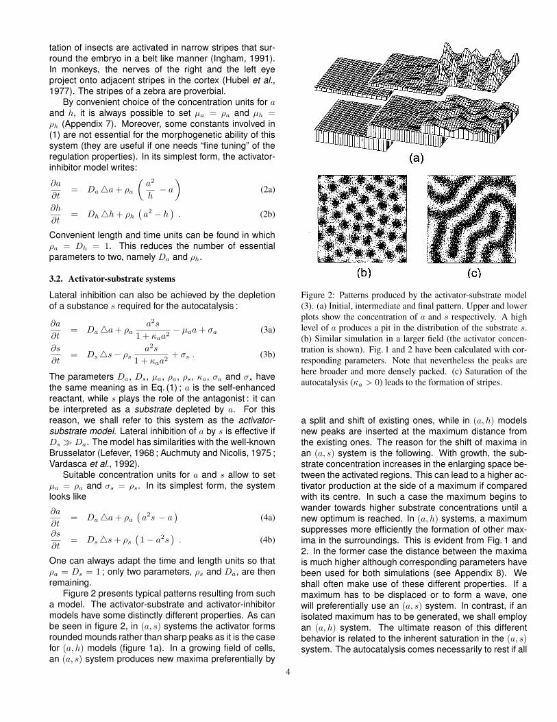
Figure 2 presents typical patterns resulting from sucha model. The activator-substrate and activator-inhibitormodels have some distinctly different properties. As canbe seen in figure 2, in (a, s) systems the activator formsrounded mounds rather than sharp peaks as it is the casefor (a, h) models (figure 1a). In a growing field of cells,an (a, s) system produces new maxima preferentially by

Figure 2: Patterns produced by the activator-substrate model(3). (a) Initial, intermediate and final pattern. Upper and lowerplots show the concentration of a and s respectively. A highlevel of a produces a pit in the distribution of the substrate s.(b) Similar simulation in a larger field (the activator concen-tration is shown). Fig. 1 and 2 have been calculated with cor-responding parameters. Note that nevertheless the peaks arehere broader and more densely packed. (c) Saturation of theautocatalysis (κa > 0) leads to the formation of stripes.

a split and shift of existing ones, while in (a, h) modelsnew peaks are inserted at the maximum distance fromthe existing ones. The reason for the shift of maxima inan (a, s) system is the following. With growth, the sub-strate concentration increases in the enlarging space be-tween the activated regions. This can lead to a higher ac-tivator production at the side of a maximum if comparedwith its centre. In such a case the maximum begins towander towards higher substrate concentrations until anew optimum is reached. In (a, h) systems, a maximumsuppresses more efficiently the formation of other max-ima in the surroundings. This is evident from Fig. 1 and2. In the former case the distance between the maximais much higher although corresponding parameters havebeen used for both simulations (see Appendix 8). Weshall often make use of these different properties. If amaximum has to be displaced or to form a wave, onewill preferentially use an (a, s) system. In contrast, if anisolated maximum has to be generated, we shall employan (a, h) system. The ultimate reason of this differentbehavior is related to the inherent saturation in the (a, s)system. The autocatalysis comes necessarily to rest if all

4

Figure 3: Position-dependent activation of a gene by an exter-nal signal simulated in a one-dimensional array of cells accord-ing to equation (5). The concentration of the autoregulatorygene product y (thin lines) is given as a function of positionand time. A primary gradient (boldface line) is used as exter-nal signal σext. Despite of the shallow signal, a sharp thresholdexists ; if exceeded, the system switches irreversibly to the highstate.

the substrate is used up. An (a, h) system obtains similarproperties if the autocatalysis saturates moderately.

3.3. Biochemical switches

A monotonic gradient based on mechanisms as de-scribed above can be maintained only if the size of thetissue is small since otherwise the time required to ex-change molecules by diffusion from one side of the fieldto the other would become too long. Indeed, as Wolpert(1969) has pointed out, all biological systems in whichpattern formation takes place are small, less than 1 mmand less than 100 cells in diameter. In an organism grow-ing beyond this size, cells have to make use of the signalsthey have obtained by activating particular genes. Oncetriggered, the gene activation should be independent ofthe evoking signal. Similarly to pattern formation, thisrequires either a direct or an indirect autocatalytic activa-tion of genes (Meinhardt, 1978).

Here is a simple example of a switch system.

∂y

∂t= ρy

y2

1 + κyy2− µyy + σext . (5)

In this equation ρy, µy and κy are constants ; σext de-scribes the external signal. In the absence of such asignal the system has two stable steady states, the lowone at y = 0 and the high one at y = (ρy +

√α)/2κyµy,

separated by an unstable steady state at y = (ρy −√α)/2κyµy, where α = ρ2y − 4κyµ

2y. If the external sig-

nal σext exceeds a certain threshold the system switchesfrom the low to the high state (Figure 3). Once the un-stable steady state is surpassed, the high state will bereached and maintained independently of the externalsignal (which could even vanish).

Somewhat more complex interactions allow thespace-dependent activation of several genes under theinfluence of a single gradient (Meinhardt, 1978). Mean-while many genes have been found with a direct regu-latory influence on their own activity (see, for instance,Kuziora and McGinnis, 1990 ; a review is given by Ser-fling, 1989), supporting the view that autoregulation is anessential element to generate stable cell states in devel-opment.

3.4. Other realizations of local autocatalysis and longranging inhibition

In the above mentioned models, self-enhancement oc-curs by direct autocatalysis (the activator production termin ∂a/∂t is proportional to a2). This direct feedback isnot necessary. As already mentioned, self-enhancementmay also result from indirect mechanisms. As an exam-ple, consider the following system :

∂a

∂t= Da4a+ ρa

(c

1 + κab2− a

)+ σa (6a)

∂b

∂t= Db4b+ ρb

(1

1 + κba2c− b

)+ σb (6b)

∂c

∂t= Dc4c+ ρc ( b− ac ) . (6c)

In this example the two substances a and b mutuallyrepress each other’s production. A small local advan-tage of a leads to a decrease of the b production. Ifb shrinks, a increases further, and so on. In this case,self-enhancement results from the local repression of arepression. The necessary long ranging inhibition is me-diated by the rapidly diffusing substance c. The latter isproduced by b but is poisonous for it. Further, c is re-moved with help of a. So, although a and b are locallycompeting, a needs b in its vicinity and vice versa. There-fore, the preferred pattern generated by such a systemconsists of stripes of a and b, closely aligned with eachother.

The interaction given above is a simple example foran important class of pattern forming reactions based onlong range activation of cell states that locally excludeeach other (Meinhardt and Gierer, 1980). According tothe theory, they play an essential role in the segmen-tation of insects (Meinhardt, 1986). Molecular analysishas confirmed this scheme ; the engrailed and the wing-less genes of Drosophila have the predicted properties[see, for instance, Ingham and Nakano (1990) or Ingham(1991) ].

The examples discussed here have been picked outof a large set of feasible morphogenetic models (Gierer,1981). They have the advantage of conceptual simplic-ity. Many other nonlinear systems have been proposed(Lacalli, 1990 ; Lyons and Harrison, 1992 ; for a broadoverview, see Murray, 1990). But, to state it once again,more important than the details of the equations are the

5

� � �

� � �

� � �

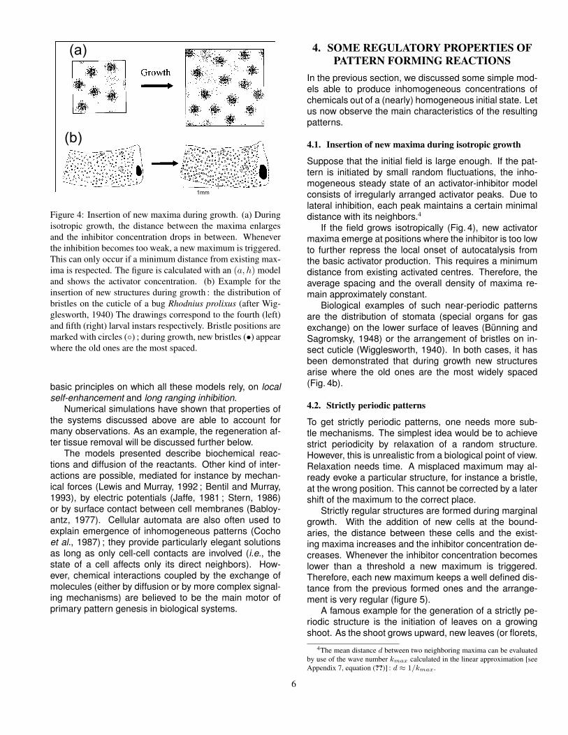
Figure 4: Insertion of new maxima during growth. (a) Duringisotropic growth, the distance between the maxima enlargesand the inhibitor concentration drops in between. Wheneverthe inhibition becomes too weak, a new maximum is triggered.This can only occur if a minimum distance from existing max-ima is respected. The figure is calculated with an (a, h) modeland shows the activator concentration. (b) Example for theinsertion of new structures during growth : the distribution ofbristles on the cuticle of a bug Rhodnius prolixus (after Wig-glesworth, 1940) The drawings correspond to the fourth (left)and fifth (right) larval instars respectively. Bristle positions aremarked with circles (◦) ; during growth, new bristles (•) appearwhere the old ones are the most spaced.

basic principles on which all these models rely, on localself-enhancement and long ranging inhibition.

Numerical simulations have shown that properties ofthe systems discussed above are able to account formany observations. As an example, the regeneration af-ter tissue removal will be discussed further below.

The models presented describe biochemical reac-tions and diffusion of the reactants. Other kind of inter-actions are possible, mediated for instance by mechan-ical forces (Lewis and Murray, 1992 ; Bentil and Murray,1993), by electric potentials (Jaffe, 1981 ; Stern, 1986)or by surface contact between cell membranes (Babloy-antz, 1977). Cellular automata are also often used toexplain emergence of inhomogeneous patterns (Cochoet al., 1987) ; they provide particularly elegant solutionsas long as only cell-cell contacts are involved (i.e., thestate of a cell affects only its direct neighbors). How-ever, chemical interactions coupled by the exchange ofmolecules (either by diffusion or by more complex signal-ing mechanisms) are believed to be the main motor ofprimary pattern genesis in biological systems.

4. SOME REGULATORY PROPERTIES OFPATTERN FORMING REACTIONS

In the previous section, we discussed some simple mod-els able to produce inhomogeneous concentrations ofchemicals out of a (nearly) homogeneous initial state. Letus now observe the main characteristics of the resultingpatterns.

4.1. Insertion of new maxima during isotropic growth

Suppose that the initial field is large enough. If the pat-tern is initiated by small random fluctuations, the inho-mogeneous steady state of an activator-inhibitor modelconsists of irregularly arranged activator peaks. Due tolateral inhibition, each peak maintains a certain minimaldistance with its neighbors.4

If the field grows isotropically (Fig. 4), new activatormaxima emerge at positions where the inhibitor is too lowto further repress the local onset of autocatalysis fromthe basic activator production. This requires a minimumdistance from existing activated centres. Therefore, theaverage spacing and the overall density of maxima re-main approximately constant.

Biological examples of such near-periodic patternsare the distribution of stomata (special organs for gasexchange) on the lower surface of leaves (Bunning andSagromsky, 1948) or the arrangement of bristles on in-sect cuticle (Wigglesworth, 1940). In both cases, it hasbeen demonstrated that during growth new structuresarise where the old ones are the most widely spaced(Fig. 4b).

4.2. Strictly periodic patterns

To get strictly periodic patterns, one needs more sub-tle mechanisms. The simplest idea would be to achievestrict periodicity by relaxation of a random structure.However, this is unrealistic from a biological point of view.Relaxation needs time. A misplaced maximum may al-ready evoke a particular structure, for instance a bristle,at the wrong position. This cannot be corrected by a latershift of the maximum to the correct place.

Strictly regular structures are formed during marginalgrowth. With the addition of new cells at the bound-aries, the distance between these cells and the exist-ing maxima increases and the inhibitor concentration de-creases. Whenever the inhibitor concentration becomeslower than a threshold a new maximum is triggered.Therefore, each new maximum keeps a well defined dis-tance from the previous formed ones and the arrange-ment is very regular (figure 5).

A famous example for the generation of a strictly pe-riodic structure is the initiation of leaves on a growingshoot. As the shoot grows upward, new leaves (or florets,

4The mean distance d between two neighboring maxima can be evaluatedby use of the wave number kmax calculated in the linear approximation [seeAppendix 7, equation (??)] : d ≈ 1/kmax.

6

� � � � � �

� � �

Figure 5: Generation of periodic structures during marginalgrowth. (a) In this simulation, the domain enlarges by additionof new cells at the upper and left border ; a periodic structureemerges. Plotted is the activator of an (a, h) model. (b) Theregular spacing of thorns on this cactus is achieved by apicalgrowth (see also section 5). The thorns are arranged alonghelices that wrap around the stem. (c) Feather primordia areregularly spaced on the back of the chicken. To position themaccurately, the chicken “simulates” growth by use of a deter-mination wave that starts from the dorsal mid line and spreadson both sides : only cells reached by the wave can initiate thedevelopment of primordia. The wave motion simulates growthby enlarging the region competent for feather production (pho-tograph by courtesy of Dr. H. Ichijo).

scales, etc.) are added sequentially near the tip, so as tomaximize the spacing with the elder ones (Adler, 1975 ;Marzec and Kappraff, 1983). Leaves emerge along spi-rals (Fig. 5b) that wrap around the stem (Coxeter, 1961 ;Rothen and Koch, 1989a, 1989b). We shall come backto this particular pattern in section 5.

It may also happen that systems which have alreadyreached a large size need to position organs in a regu-lar fashion. This can occur by a “simulated” growth. Theproperty of a tissue may change in a wavelike mannerfrom a state noncompetent to a state competent for pat-tern formation. Although many cells are already present,pattern formation can take place only in a small portionof the field. With the enlargement of the competent re-gion more and more maxima are formed that keep pre-cise distances to the existing ones. An example is theformation of the regularly spaced feather pattern in chick(Fig. 5c). Feather primordia begin their differentiationbehind a competence wave that starts from the dorsal

Figure 6: Regeneration with polarity reversal. (a) Experimen-tal observation : the early blastula of a sea urchin is cut in twohalves. Cells close to the wound are vitally stained (dottedregion) to determine later the original orientation. Both partsregenerate a complete embryo. They are mirror-symmetric,so that in one fragment the polarity must have been reverted(Horstadius and Wolsky, 1936). (b) Simulation by an activator-inhibitor model. The abscissa scale gives the position along thedorso-ventral axis of the blastula, in % of the animal length.After separation, the high residual inhibitor concentration (- - -) in the non-activated part (arrow) leads to regeneration of theactivator (—) at the opposite end of the field. The distributionbefore and after cutting is shown, as well as the newly formedsteady state.

mid line and spreads to both sides of the back. Exper-iments (Davidson, 1983a, 1983b) have clearly demon-strated that lateral inhibition is involved in the formationof the regularly spaced feather primordia. We shall meeta similar phenomenon in section 5 when discussing theformation of the Drosophila eye.

4.3. Regeneration properties and polarity

Many biological systems can regenerate missing parts.The models discussed above are able to account for thisproperty. We shall use the activator-inhibitor model andmodifications of it to demonstrate this feature and com-pare them with biological observations.

After partition of an early sea urchin embryo bothfragment regenerate complete embryos. By vital stain-ing during separation it has been shown that both em-bryos obtain a mirror-image orientation with respect toeach other (Fig. 6). According to the model, in the non-activated fragment the remnant inhibitor decays until anew activation is triggered. The polarity of the resultingpattern depends on the distribution of the residual acti-vator and inhibitor in the fragment. A polarity reversal,as in the case of the sea urchin mentioned above, willtake place if the residual inhibitor gradient is decisive forits orientation. It is the region with the lowest inhibitor

7

Figure 7: Regeneration with maintained polarity. (a) After cut-ting, fragments of Hydra regenerate. The original apical-basalpolarity is maintained. (b) Model based on Eq. (7). The ab-scissa gives, in % of the full length, the position along the bodyaxis. The inhibitor is assumed to have a feedback on the sourcedensity b (- - -) which describes the general ability of the cellsto perform the autocatalysis. This source density, having a longtime constant, does not change considerably during regenera-tion of the activator-inhibitor pattern. Regions closer to theoriginal head have an advantage in the competition for headformation and the new maximum of the activator a (—) is reli-ably triggered in the region which was originally closest to theapical side.

concentration, i.e., the region most distant to the origi-nally activated site that wins the competition to becomeactivated.

In many other systems the polarity is maintained.The fresh water polyp Hydra (Wilby and Webster, 1970 ;Wolpert et al., 1971 ; Macauley-Bode and Bode, 1984)and planarians (Flickinger and Coward, 1962 ; Goss,1974 ; Chandebois, 1976) are examples. The mainte-nance of polarity implies that the same tissue can regen-erate either a head or a foot depending whether this par-ticular tissue is located at the apical or the basal end ofthe fragment which has to regenerate. Morgan (1904)interpreted this phenomena in that a graded stable tis-sue property exists. It provides a graded advantage inthe race to regenerate a removed structure. During headregeneration, for instance, those cells will win that wereoriginally closest to the removed head.

In terms of the activator-inhibitor mechanism, a sys-tematic difference in the ability to perform the autocatal-ysis must exist. We call this property the source density.Detailed simulations for hydra (Meinhardt, 1993) haveshown that the source density must have approximatelythe same slope as the inhibitor. However, while time con-stants of the activator and inhibitor are in the range of a

few hours, a major change of the source density requiresapproximately two days (Wilby and Webster, 1970).

In the following model, a feedback exist from the in-hibitor h onto the source density b. Therefore, in thecourse of time, a long ranging gradient not only of hbut also of b will be established. Whenever the systemis forced to regenerate, the residual distribution of b en-sures the maintenance of polarity.

∂a

∂t= Da4a+ ρa

[b

(a2

h2+ σa

)− a

](7a)

∂h

∂t= Dh4h+ ρh

(a2 − h

)(7b)

∂b

∂t= ρb (h− b ) . (7c)

As can be verified in (7c), at equilibrium, b = h. Thus, theself-enhancement term ba2/h2 in the activator equation(7a) reduces to a2/h as in the usual activator-inhibitormodel (1). Since the removal rate ρb is small comparedto ρa and ρh, b preserves the polarity when the animalis dissected : due to enhancement of autocatalysis by b,the activator a builds up again in each half at the siteof highest b concentration. The position of the relativehighest source density plays the crucial role as to wherethe new activator maximum will be formed. This insuresmaintenance of the initial polarity (Fig. 7).

The feedback of h onto the source density b has an-other very important effect, it helps to suppress the initi-ation of secondary maxima. This is required if a singlestructure, for instance a single head, should be main-tained in a system despite of substantial growth. Since,with increasing distance from the existing maxima, cellshave a lower and lower source density, it becomes lesslikely that these cells overcome the inhibition spreadingfrom an existing maximum.

In Hydra, treatment with diacylglycerol (a substanceinvolved in the second messenger pathway) causes su-pernumerary heads (Muller, 1990). From detailed obser-vations and simulations one can conclude that this sub-stance is able to increase the source density in a dra-matic way. Since the source density becomes high ev-erywhere, the so-called apical dominance of an existinghead is lost and supernumerary heads can be formed.These heads keep distance from each other since thespacing mechanism enforced by the inhibitor alone is stillworking. The model agrees with many other experimen-tal results, including the existence of a critical size (seeAppendix 7) below which the animal is unable to regen-erate (Shimizu et al., 1993).

5. FROM SIMPLE GRADIENTS TOCOMPLEX STRUCTURES

So far we have considered models able to generate inho-mogeneous distributions of substances out of an initiallyuniform state. By combining several systems of this kindvery complex structures can be formed in a reproducible

8

way. Central is the idea of hierarchy. A first system A es-tablishes a primary pattern that is used to modify and trig-ger a second system B. The feedback in the reverse di-rection, of B onto A, is assumed to be weak (this greatlysimplifies the treatment of these nonlinear systems andmakes the comprehension of their properties easier).

To fix the ideas, suppose that both A and B areactivator-inhibitor systems (aA, hA) and (aB , hB). Itis then natural to assume that parameters ρaB , ρhB

,σaB . . . of B are functions of the chemical concentrationsof A. The couplings which proved to be the simplest andthe most efficient in simulations consist to modify eitherthe cross-reaction parameter ρaB or the basic (activator-independent) production σaB of the second activator aB .The two following thumb rules are helpful.

• If the second system has to respond dynamicallyto any change of the first one, one will preferen-tially alter the value of ρaB . This ensures that anychange in A is repercuted on B [in terms of thefigure ?? in Appendix 7, one would choose the cou-pling function ρaB in such a way that the systemB shifts under the pressure of A from the regionH of the stability diagram (where B has no patternformation ability) into the domain I (where inhomo-geneities can be amplified) ].

• If A has just to trigger B, the coupling between thetwo systems is achieved by the basic productionσaB . The structure developed by B is then stableeven if, later, A vanishes.

Other kinds of interactions are conceivable as well. Forinstance, cells could change the communication withtheir neighbors by opening or closing gap junctions ; thiscan be modeled by altering the diffusion constants un-der the influence of a second patterning system. In thefour examples developed below we restrict, however, theinteraction between systems to the two rules mentionedabove. The two first systems are relatively simple modelsof animal coat patterns and of reticulated structures. Thelast two examples are more complex and describe inter-action that leads to the precise arrangement of differentlydetermined cells in a strictly periodic way. The eye forma-tion in Drosophila and organ genesis in a growing plantwill be used as biological counterparts.

5.1. Animal coat patterns

The variability and complexity of animal coat patterns hasattracted many biologists. Models can be found for thecoloration of butterfly wings (Nijhout, 1978, 1980 ; Mur-ray, 1981), zebra stripes (Bard, 1981 ; Murray, 1981), pat-terns on snake skin (Cocho et al., 1987 ; Murray and My-erscough, 1991) or on sea shells (Meinhardt and Klinger,1987 ; Ermentrout et al., 1989). We present hereaftera simple reaction-diffusion mechanism which allows alarge variability of patterns, ranging from the spots of thecheetah to the reticulated coat of giraffes.

� � � � � �

Figure 8: Analogy of the giraffe pattern with Dirichlet do-mains. (a) Side of a giraffe (Giraffa camelopardalis reticu-lata). The pattern is formed by convex polygons separatedby thin lines (photograph kindly provided by O. Berger). Theformal resemblance with Dirichlet domains is suggestive. (b)Construction and definition of Dirichlet domains. Given a set{P1, . . . , Pn} of points belonging to a surface S, one drawsthe perpendicular bisectors between neighboring points. Theconvex envelop surrounding a center Pi delimits its associ-ated Dirichlet domain Di. By construction, Di contains allthe points of the surface S nearer to Pi than to any other Pj(j 6= i).

In mammals, hair pigmentation is due to melanocyteswhich are supposed to be uniformly distributed in thederma. Whether they produce melanin (which colorshairs) or not is believed to depend on the presence ofsome unknown chemicals whose pattern is laid downduring the early embryogenesis (Bard, 1977).

Let us start with a short description of the giraffecoat. Figure 8 show the similarity between the polygo-nal shaped spots that cover the animal and Dirichlet do-mains. This suggests that a reaction-diffusion system isat work in the giraffe’s coat that is able to produce Dirich-let polygons. Consider a surface S and points P1, . . ., Pnrandomly scattered on it. Suppose that each Pi initiatesat a given time a chemical wave which spreads uniformlyto all directions. The system should be so that, if twowaves encounter, they annihilate each other. The linesalong which annihilation occurs defines the envelops ofthe Dirichlet domains around the initial centers Pi. Thefollowing reaction-diffusion system fulfils these require-ments :

∂a

∂t= Da4a+ ρa

[a2s

1 + κaa2− a

](8a)

∂s

∂t= Ds4s+

σs1 + κsy

− ρsa2s

1 + κaa2− µss (8b)

∂y

∂t= ρy

y2

1 + κyy2− µyy + σya (8c)

One recognizes a modified activator-substrate model(a, s) combined with a switching system y. Melanocytesactivity is given by y : y = 1 corresponds to cells produc-ing melanin, while melanocytes with y = 0 don’t. The

9

state y of each pigment cell is determined by its exposi-tion to the morphogen a. To insure that a doesn’t producea stationary pattern but spreads like a wave, the diffusionconstant of s should not be too large when compared tothe one of a.

The system works in the following way : initially y = 0,a = 0 and s = so everywhere, except on some randomlyscattered points5 Pi where a = ao ; this high value ofa switches y from 0 to 1 at Pi due to the source termσya in (8c). On the other hand, due to the depletion of sand to its low diffusion constant Ds, high a regions shifttoward zones where the substrate is abundant : a-wavespropagate over the surface. When two such waves getclose, they annihilate each other due to the depletion ofsubstrate s. Owing to its switching nature, y needs theactivator a just for being triggered. Once a has vanished,the state of y remains stable. Note that y has a negativefeedback on the production of s in (8b) : in regions wherey has switched on, it is no longer necessary to wasteenergy to produce the substrate s any more.

Figure 9a presents the result of a simulation. Thesimilarity with the coat of a giraffe is obvious. Straightlines with nearly constant thickness delineate irregularpolygons ; earlier models proposed for giraffe patterns(Murray, 1981, 1988) produce rather spots comparableto Fig. 9c.

According to the parameter values, the model (8) pro-duces a variety of patterns related to Dirichlet domains.For instance, if the removal rate of s is low enough,regions where a doesn’t vanish subsist ; the systemreaches then a stable configuration where the activatora remains activated along circular rings or “half-moons”centered on the initiating points Pi (Fig. 9b). Conversely,if the consumption of s is too high, the a-waves cannotspread very far and die before they meet : randomly scat-tered spots are formed (Fig. 9c). In that situation, theresulting pattern has much similarities with the one de-scribed by Murray (1981, 1988).

The coats of mammals have been taken as illustra-tions. Fishes, snakes and insects show similar patterns.It is appealing to imagine that they may all be based on acommon mechanism involving Dirichlet domains, as dis-cussed above.

5.2. Reticulated structures

Polygonal patterns are also common in other biologicalsystems. The fine veins of the wing of a dragonfly or theprojection areas of mice sensory whiskers on the brainare examples (Fig. 10).

A crucial property of the system discussed in the pre-ceding paragraph is that the pattern, once formed, isfixed. For instance, no new lines can be inserted dur-

5In principle the centers Pi could be laid down by a primary pattern for-mation mechanism (aP , hP ) like the one used to produce figure 1a . Thesepoints would then activate the production of a by means of an additional termσaaP in Eq. (8a). We skip this step.

Figure 9: Simulation with the system (8). The dot density isproportional to the concentration of y. According to the pa-rameter set, the resulting pattern will have similarities with theone observed on the coat of giraffes (Giraffa camelopardalisreticulata) (a), of leopards (Panthera pardus) (b) or of chee-tahs (Acinonyx jubatus) (c).

ing growth to subdivide a large polygon into two smallerones. This is appropriate for the giraffe coating as in-dicated by the large size of the polygons. For other sys-tems such as the wing of the dragonfly mentioned above,it is to be expected that the final pattern is not produced ina single step at a particular moment of the development ;it is rather likely that, at an early stage and in a smallfield, a simple pattern is laid down. In analogy to theDrosophila wing venation (Diaz-Benjumea et al., 1989 ;Garcia-Bellido et al., 1992), we assume that the posi-tions of the main veins of the dragonfly wing are genet-ically determined ; the finer ones are presumably addedlater in order to strengthen the growing structure and soas to keep approximately constant the size of a domainenclosed by veins.

The following model has this property. It relies uponhierarchical interactions of two systems. A first (a, s)activator-substrate system produces a pattern of activa-

10

tor mounds (see Fig. 2a) :

∂a

∂t= Da4a+ ρa

(sa2

1 + κab2− a

)+ σa (9a)

∂s

∂t= Ds4s− ρs

(sa2

1 + κab2

)+ σs . (9b)

This primary pattern triggers an activator-inhibitor system(b, h) producing boundaries around the mounds of a.

∂b

∂t= Db4b +

ρb

[s2

1 + κbab2

(b2

h+ σb

)− b

](10a)

∂h

∂t= Dh4h+ ρh

(b2 − h

). (10b)

The a-concentration modifies the saturation value of theactivator b in Eq. (10a). A high value of a makes this satu-ration so strong that the (b, h) system is set off. In regionsof low a, it’s the other way round : the saturation becomesweak enough so that the (b, h) system triggers the forma-tion of a stripe-like boundary. This effect is enhanced bythe substrate s, through the term ρbs

2 in (10a). In otherwords, the stripes will appear along sites with high con-centration of s, in regions that are most distant from themaxima of a. Due to the action of h, the stripes becomesharp. The weak feedback of b onto a in equation (9a) isnot absolutely necessary but speeds up the developmentof the structure. The model has size regulation proper-ties. New boundaries are inserted whenever a domainbecomes too large. This has the following reason. Withgrowth, the distance between the a maxima increases. Ifa certain distance is surpassed, a maximum splits intotwo and displacement towards higher substrate concen-tration follows. Between these two maxima, a new regionwith high substrate concentration appears that, in turn,initiates a new b line. Such a process can be observed infigure 10c.

As a possible application of the mechanism (9)–(10)let us shortly mention the barrel formation in mouse brain(Steindler et al., 1989 ; Jacobson, 1991). The facial vib-rissae of the mouse project on the primary somatosen-sory cortex (Fig. 10b). The mapping on the brain mirrorsthe arrangement of whiskers on the mouse face : two ad-jacent vibrissae project on neighboring sites in the cor-tex ; the domain connected to a given whiskers is calledbarrel. The shape of the barrels can be visualized bya labelling with tenascin specific antibodies. During thefirst postnatal days, the barrel pattern has dynamic prop-erties : removal of vibrissae disrupts the formation of theassociated barrels. The model gives a good descriptionof such dynamic effects if one admits that the autocat-alytic production rate of activator a is linked to neural ex-citation by the whiskers. Destruction of the latter leads toa reduction of neural excitation, to a decrease of a andso, to the resorption of the associated barrel whose areais then invaded by its neighbors.

Figure 10: Polygonal structures. (a) The left posterior wing ofa dragonfly (Libellula depressa) is strengthened by a fine andelegant network of veins (picture after Seguy, 1973). The posi-tions of the larger veins are presumably genetically coded. Ac-cording to the model, finer veins are produced during the wingdevelopment ; during growth, their insertion tends to keep con-stant the size of the enclosed domains. (b) Experimentally ob-served barrel pattern in the mouse somatosensory cortex. Thedotted regions correspond to domains labelled by an antibodyagainst J1/tenascin (after Steindler et al., 1989).(c) Simulationbased on the system (9)–(10) in a two dimensional domain.The density of dots is proportional to the concentration of b.One can see the completion of a new boundary between twodomains (arrow).

5.3. The facetted eye of Drosophila flies

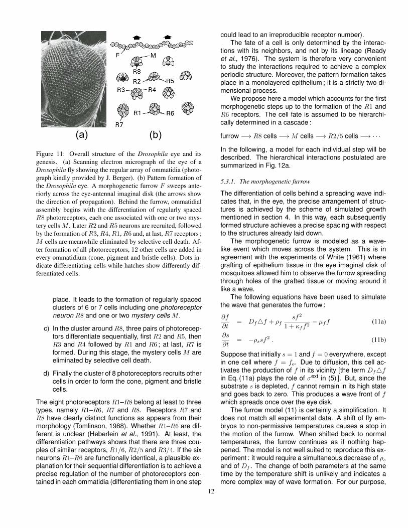
As an example of a complex but very regular periodicstructure, we shall now discuss the formation of thefacetted eye of the fruit fly Drosophila melanogaster. Theeye is derived from the eye-antennal imaginal disk.6 Itconsists of a very regular array of about 700 ommatidia(Fig. 11a). Each ommatidium is formed by the precise ar-rangement of 20 cells among which 8 are photoreceptorneurons named R1, . . ., R8. These clusters of 20 cellshave well defined polarity and orientation in respect tothe main body axis.

The molecular basis of eye formation has been ex-tensively studied over the last years. For comprehen-sive reviews, see for instance Tomlinson (1988) or Baslerand Hafen (1991). The model presented hereafter repro-duces essential aspects of this pattern formation.

The following steps play a crucial role (figure 11b).

a) A wave moves from posterior to anterior across theeye imaginal disk. It causes a slight deformation inthe tissue, the morphogenetic furrow.

b) Within the furrow, a first morphogenetic event takes6In Drosophila larvae, imaginal disks are nests of epithelial tissue which

differentiate at metamorphosis. Legs, wings, antennae, eyes derive from imag-inal disks (Alberts et al., 1989).

11

� � � � � �

Figure 11: Overall structure of the Drosophila eye and itsgenesis. (a) Scanning electron micrograph of the eye of aDrosophila fly showing the regular array of ommatidia (photo-graph kindly provided by J. Berger). (b) Pattern formation ofthe Drosophila eye. A morphogenetic furrow F sweeps ante-riorly across the eye-antennal imaginal disk (the arrows showthe direction of propagation). Behind the furrow, ommatidialassembly begins with the differentiation of regularly spacedR8 photoreceptors, each one associated with one or two mys-tery cells M . Later R2 and R5 neurons are recruited, followedby the formation ofR3,R4,R1,R6 and, at last,R7 receptors ;M cells are meanwhile eliminated by selective cell death. Af-ter formation of all photoreceptors, 12 other cells are added inevery ommatidium (cone, pigment and bristle cells). Dots in-dicate differentiating cells while hatches show differently dif-ferentiated cells.

place. It leads to the formation of regularly spacedclusters of 6 or 7 cells including one photoreceptorneuron R8 and one or two mystery cells M .

c) In the cluster around R8, three pairs of photorecep-tors differentiate sequentially, first R2 and R5, thenR3 and R4 followed by R1 and R6 ; at last, R7 isformed. During this stage, the mystery cells M areeliminated by selective cell death.

d) Finally the cluster of 8 photoreceptors recruits othercells in order to form the cone, pigment and bristlecells.

The eight photoreceptors R1–R8 belong at least to threetypes, namely R1–R6, R7 and R8. Receptors R7 andR8 have clearly distinct functions as appears from theirmorphology (Tomlinson, 1988). Whether R1–R6 are dif-ferent is unclear (Heberlein et al., 1991). At least, thedifferentiation pathways shows that there are three cou-ples of similar receptors, R1/6, R2/5 and R3/4. If the sixneurons R1–R6 are functionally identical, a plausible ex-planation for their sequential differentiation is to achieve aprecise regulation of the number of photoreceptors con-tained in each ommatidia (differentiating them in one step

could lead to an irreproducible receptor number).The fate of a cell is only determined by the interac-

tions with its neighbors, and not by its lineage (Readyet al., 1976). The system is therefore very convenientto study the interactions required to achieve a complexperiodic structure. Moreover, the pattern formation takesplace in a monolayered epithelium ; it is a strictly two di-mensional process.

We propose here a model which accounts for the firstmorphogenetic steps up to the formation of the R1 andR6 receptors. The cell fate is assumed to be hierarchi-cally determined in a cascade :

furrow −→ R8 cells −→M cells −→ R2/5 cells −→ · · ·

In the following, a model for each individual step will bedescribed. The hierarchical interactions postulated aresummarized in Fig. 12a.

5.3.1. The morphogenetic furrow

The differentiation of cells behind a spreading wave indi-cates that, in the eye, the precise arrangement of struc-tures is achieved by the scheme of simulated growthmentioned in section 4. In this way, each subsequentlyformed structure achieves a precise spacing with respectto the structures already laid down.

The morphogenetic furrow is modeled as a wave-like event which moves across the system. This is inagreement with the experiments of White (1961) wheregrafting of epithelium tissue in the eye imaginal disk ofmosquitoes allowed him to observe the furrow spreadingthrough holes of the grafted tissue or moving around itlike a wave.

The following equations have been used to simulatethe wave that generates the furrow :

∂f

∂t= Df4f + ρf

sf2

1 + κff2− µff (11a)

∂s

∂t= −ρssf2 . (11b)

Suppose that initially s = 1 and f = 0 everywhere, exceptin one cell where f = fo. Due to diffusion, this cell ac-tivates the production of f in its vicinity [the term Df4fin Eq. (11a) plays the role of σext in (5) ]. But, since thesubstrate s is depleted, f cannot remain in its high stateand goes back to zero. This produces a wave front of fwhich spreads once over the eye disk.

The furrow model (11) is certainly a simplification. Itdoes not match all experimental data. A shift of fly em-bryos to non-permissive temperatures causes a stop inthe motion of the furrow. When shifted back to normaltemperatures, the furrow continues as if nothing hap-pened. The model is not well suited to reproduce this ex-periment : it would require a simultaneous decrease of ρsand of Df . The change of both parameters at the sametime by the temperature shift is unlikely and indicates amore complex way of wave formation. For our purpose,

12

Figure 12: Simulation of the eye development. (a) Scheme ofthe hierarchical interactions used in the model. The furrow Finduces regularly spaced R8 neurons. These are needed to de-velop M cells. Later, R8 and M cells cooperate to trigger thedifferentiation of R2 and R5 neurons. At last, R8 and R2/5neurons induce the formation of R3/4 and R1/6 receptors.Except of the R8 spacing mechanism that involves long rang-ing inhibition, all interactions are assumed to be mediated bycell-cell contacts. (b) The structure resulting from the model.The morphogenetic furrow F moves across the eye disk (thearrows show the direction of spreading). It initiates the differ-entiation of neural cells : a regular array of R8 photoreceptorsdevelops behind it. Mystery cells M differentiates immedi-ately anteriorly to R8 receptors. Later R2 and R5 are formed.The differentiation ofR3/4 andR1/6 follows (these cells havenot been plotted for reasons of clarity).

however, the form (11) is sufficient since we only need itas a signal for beginning the neuronal differentiation.

5.3.2. The R8 photoreceptors

The morphogenetic wave triggers the differentiation ofneuronal cells R8. Experimental data point out that lat-eral inhibition is essential for proper R8 spacing (Bakeret al., 1990 ; Harris, 1991). So R8 cells are best modeledby an activator-inhibitor couple (aR8, hR8) :

∂aR8

∂t= DaR8

4aR8 + ρaR8

(a2R8

hR8− aR8

)+σaR8

f (12a)∂hR8

∂t= DhR8

4hR8 + ρhR8

(a2R8 − hR8

). (12b)

Cells begin to differentiate after they have been exposedto the morphogenetic wave. In the model, activation de-pends on the basic production term σaR8

f in Eq. (12a).Due to the lateral inhibition via hR8 only some cells be-come fully activated and differentiate into R8 photorecep-tors (Fig. 12b). These cells have a precise spacing withrespect to the previously activated R8 cells.

The diffusion range of the inhibitor hR8 is supposed tobe of the order of several cell diameters. In the model this

is the only substance with such a long diffusion range.All subsequently determined cells (M , R2, R5, etc.) dif-ferentiate under the influence of local interactions re-layed by direct contact with the R8 cells (Banerjee andZipursky, 1990).

5.3.3. Mystery cells M

The mystery cells M got their names because biologistsare, until now, unable to assign to them a role duringthe eye formation ; some hours after their differentiation,mystery cells die. The model suggests that M cells areused in conjunction with R8 neurons to induce a localpolarity : like an arrow, the couple R8–M points to thefurrow. This local remembrance is thought to be crucialfor the correct positioning of subsequent photoreceptors,especially of R2/5. According to the model, the M cellacts, in conjunction with R8, as an initial organizer forommatidial development by determining the primary ori-entation of the cell cluster and by restricting the numberof cells which can choose the R2/5 fate. Perturbationsof the furrow motion, as in White’s (1961) experiment,should lead to observable alterations of the initial clusterorientation. This could be a test for the model.

The following interaction allows the activation of theM cell adjacent to the R8 cell.

∂aM∂t

= DaM 4aM + ρaM cM (aR8)a2MhM

−µaMaM + σaM f (13a)∂hM∂t

= DhM4hM

+ρhM

(a2M − hM

)+ σhM

. (13b)

The function cM (aR8) simulates the transmission of a sig-nal by cell-cell contact between the putative M cell andthe R8 neuron : this signal could, for instance, be relayedby proteins laying on the cellular membrane of R8 neu-rons. In the simulation, we chose

cM (aR8) =aR8

1 + κMa2R8

.

Due to this function, aR8 is required for the initiation ofthe mystery cell ; but in reason of a disfavoring effect atvery high aR8 concentrations, it is not the R8 cell itselfbut a neighboring cell in which aM activation takes place.The term σaM f which couples the production of aM withthe furrow selects which of the R8 neighbors is chosento become a mystery cell. The trail of the f -wave makessure that M cells differentiate anteriorly to R8 neurons,so that the couple R8–M is like an arrow pointing to thefurrow.

In the simulations, the precise positioning of M ante-riorly to R8 is delicate ; fluctuations disrupt easily this or-der. It could be that a similar sensitivity exists in nature.Experimentally it has been observed that cell movementsplay an important role in local rearrangement during theeye genesis (Tomlinson, 1988). In this way, small errors

13

in the precise positioning of the M cells could be cor-rected.

5.3.4. Recruitment of R2/5, R3/4 and R1/6 neurons

It is generally accepted that the subsequent differentia-tion of the R2/5 and later of the R3/4 and R1/6 pho-toreceptors is a consequence of cell-cell contacts. In themodel, interactions with the R8 and M cells directs anundifferentiated cell to choose the R2/5 fate. Conversely,newly formed R2/5 neurons inhibit their neighbors to fol-low the same pathway. Later, other cells differentiate intoR3/4 and R1/6 receptors, due to contact with R8 andR2/5 neurons. Again, R3/4 and R1/6 receptors preventother cells in their vicinity from choosing the same fate.

These considerations suggest that equations govern-ing the R2/5, R3/4 and R1/6 neuronal pathway are ofthe very same nature as those for R8 and M cells. Forinstance, the R2/5 receptors are described by

∂aR2

∂t= DaR2

4aR2 + ρaR2cR2(aR8, aM )

a2R2

hR2

−µaR2aR2 + σaR2

(14a)∂hR2

∂t= DhR2

4hR2

+ρhR2

(a2R2 − hR2

)+ σhR2

. (14b)

Cells with a high aR2 concentration become R2/5 neu-rons (Fig. 12c). The function cR2 relays a signal from R8and M cells to the presumptive R2/5 photoreceptors :

cR2(aR8, aM ) =aR8

1 + κR2a2R8

· aM1 + νR2a2M

.

Note that cR2 depends on the product of two signals.Both interactions with R8 and with M are simultaneouslyrequired to induce the differentiation of R2/5 receptors.

Further differentiation of R1/6 and R3/4 photorecep-tors uses the same scheme except that cR2(aR8, aM ) isreplaced by a function cR3(aR8, aR2) which mimics sur-face contact with R8 and R2/5 neurons.

5.3.5. Abnormal eye patterns

Many mutations are known which alter the structure ofthe compound eye. Four of them, rap (Karpilov et al.,1989), Ellipse (Baker and Rubin, 1989), Notch (Har-ris, 1991 ; Markopoulou and Artavanis-Tsakonas, 1991)and scabrous (Baker et al., 1989) affect the positioningand differentiation of R8 cells. Based on the pheno-types of Ellipse and scabrous flies, we suggest that El-lipse is linked to the R8-activator aR8, while the diffusiblemolecule encoded by scabrous may be the correspond-ing inhibitor hR8.

In scabrous mutants, the R8-inhibition is reduced.This is modeled by increasing the value of ρhR8

inEq. (12b). For a given concentration of aR8, more hR8

is produced and this, in turn, decreases the amount ofboth aR8 and hR8 ; as a consequence, R8 cells are less

spaced, irregularly distributed and sometimes two R8neurons are fused, as observed in scabrous mutants.

Notch mutants exhibit the same kind of reduced R8spacing. Notch encodes for a transmembrane proteinthat is believed to be a receptor for several extracellu-lar signals. Among them is the signal relayed by thescabrous protein. In this sense, the parameter ρaR8

hasto be a function of Notch. The model does not explicitlytake this Notch-dependance into account. But a mutationmaking the Notch protein less effective for the receptionof the scabrous inhibition signal could decrease the valueof ρaR8

in Eq. (12a). Less activator is then produced ; thisdecreases also the hR8 concentration and R8 are formedtoo close to each other, as observed in Notch mutant.

The opposite result is achieved by increasing ρaR8:

this enhances the production of aR8, leading this timeto an abnormally wide R8 spacing. It is interesting tonote that the Ellipse mutation is believed to overactivatethe gene responsible forR8 differentiation, in accordancewith the considerations above.

It should be noted that the regulatory behaviors men-tioned above are nontrivial consequence of the model :if more inhibitor molecules are produced per activatormolecules, one achieves a decrease of the inhibitor con-centration. This results from the nonlinear cross-reactionbetween these two chemicals. This kind of regulatory be-havior is not unique to eye development. Mutants havebeen found in hydra, where a decrease of the head in-hibitor production rate induces surprisingly an increaseof the head-bud spacing (Takano and Sugiyama, 1983).

Another mutation that disrupts the eye assembly isrough (Heberlein et al., 1991). In rough mutants, devel-opment of ommatidia occurs normally up to R2/5. ButR3/4 neurons fail their differentiation. It has been sug-gested (Tomlinson et al., 1988 ; Basler et al., 1990) thatrough controls in R2/5 photoreceptors the signal that in-duces the R3/4 cell fate. In the model we would identifythe activity of rough with the signal cR3(aR8, aR2). Exper-imentally it has been observed that rough expression ishigh, first, in the morphogenetic furrow and, later, in R2/5and R3/4 cells (Kimmel et al., 1990). This correspondsto the expectation of the model.

The model is already quite complex but is certainlyan oversimplification. For instance, the exchange of in-formation between the cells is much more sophisticatedthan that just a substance leaking through some holesinto neighboring cells. A plausible mechanism wouldrather involve signalling molecules that are inserted intothe membrane of one cell type and receptor moleculesexposed on other cells. “Relay molecules” will then trans-mit the signal from the cell surface to the nucleus. There,transcriptional regulation takes place that is ultimately re-sponsible for the choice of the pathway. Nevertheless,this signal transduction is presumably a more or less lin-ear chain of events, so that the approximation by a singlesubstance exchanged by diffusion is reasonable.

Although the model seems complex, its building fol-14

lows a straightforward way, consisting of the successiveaddition of elements whose properties are well under-stood. These “building blocks” include wave formation,production of regular structures by simulated growth andfate induction in a neighboring cell. Though each singleelement has well defined characteristics, one learns fromthese models where the critical steps are. For instance,it turned out that the generation of polarity in the periodicarray of receptors is a delicate step which is facilitated bythe addition of a mystery cell.

5.4. Positioning mechanisms during plant growth

As a last example of a complex structure, we describe amodel that allows the precise positioning of organs dur-ing the development of plants.

Plant growth mainly occurs by cell division in special-ized tissues called meristems. The shoot apex meristemis a cone of undifferentiated cells located at the tip ofstems ; its cells undergo frequent mitosis. Somewhat be-hind the tip, the primordia are formed (Fig. 13). Thesewill develop into leaves or flower organs. The determina-tion of the positions at which primordia appear is believedto involve some inhibition mechanism (Schoute, 1913 ;Thornley, 1975 ; Marzec and Kappraff, 1983 ; Koch et al.,1994). Several models have been proposed to explainthe precise positioning of primordia. They are based ei-ther on the exchange of diffusible molecules (Meinhardt,1982 ; Yotsumoto, 1993 ; Bernasconi, 1994) or on stressand pressure in the tissue (Adler, 1974, 1977a, 1977b ;Green and Poethig, 1982). A pattern very similar to phyl-lotaxis can be generated by physical ingredients only.Under suitable conditions, swimming and each other re-pelling droplets of a magnetic fluid also produce helicalarrangement (Douady and Couder, 1992).

Although a single activator-inhibitor system is able toaccount for the basic modes of leaf arrangement (distic-hous, decussate, helical) (Mitchison, 1977 ; Richter andSchranner, 1978 ; Meinhardt, 1982), it is easy to see thatmore complicated systems are involved. We shall dis-cuss the necessary extensions in several steps.

Leaf initiation can take place only in a small zone atsome distance from the tip of a growing shoot. Further,a signal must be available which specifies where apicalmeristem is located. This suggests that at least two pat-tern forming systems are involved. The first one deter-mines the position of the meristem. The second systemgenerates leaves. The latter is controlled by the first one :on one hand, the meristem system represses leave ini-tiation at the tip but, on the other hand, it generates theprecondition for this process in its vicinity (Fig. 13). Thisis analogous to the Drosophila eye development where amystery cell M can only emerge in the neighborhood ofa photoreceptor R8. Therefore, leaf initiation is restrictedto a narrow zone at the border of the apical meristem. Asimilar process takes place in the freshwater polyp Hy-dra : initiation of tentacles takes place only in a whorl

around the mouth opening (Meinhardt, 1993).However, even this more complex model is insuffi-

cient. After leaf initiation, axillary meristems are formedadjacent to the leaf primordia. They are always locatedon the side pointing towards the tip of the shoot. Thesemeristematic regions don’t lead immediately to cell pro-liferation but they can give rise to a new shoot after theoriginal shoot is removed. Moreover, leaves obtain verysoon a polarity on their own in that their upper and lowersurface become different from each other [this process isprobably induced by the neighborhood of the leaf (Sus-sex, 1955) ]. The situation is therefore similar to the onedescribed above for eye development since several dif-ferent structures are generated in a precise periodic ar-rangement and with a predictable orientation.

A key for the understanding of this complex patternis its modular character (Lyndon, 1990). The elemen-tary unit (the module) produced by a growing shoot con-sists of a node and internode segment associated witha leaf primordium and an axillary bud (Fig. 13). Leavesare always located at the top of a module, in the nodalregion ; axillary buds differentiate close to leaves and im-mediately above them. Stem elongation takes place inthe internodal region (Zobel, 1989a, 1989b).

In the following, we shall propose a model based onthis modular structure that accounts for the precise ax-ial and azimutal positioning of leaf primordia and axillarybuds on the stem. The model also includes a control ofmeristematic activity after tip removal. Since most of theprimary morphogenetic events affect only one or two sur-face cell layer(s), we shall idealize the plant as a hollowcylinder.

5.4.1. The apical shoot meristem

The apical meristem located at the tip of stems repressesthe activity of the buds in its vicinity. The apical domi-nance decreases as the distance between the apex anda given bud increases with growth. This regulation isknown to be mediated by phytohormones like auxins(Snow, 1940 ; Kuhn, 1965).

We take into account two properties of the meris-tem. The first one, modeled by a switch system aM ,tells whether a cell belongs to the apical meristem type(aM = 1) or not (aM = 0). A second switching systemaA controls whether the meristem is active, i.e., whethercells are undergoing frequent mitosis (aA = 1) or stay ina latent state (aA = 0). A further substance hA mediatesthe repression of axillary bud activity. It is produced in ac-tive shoot meristems and could correspond to the phyto-hormone mentioned above. It must be of very long rangein order to suppress the meristematic activity in distantaxillary buds. This rapid spread must not result fromdiffusion. Indeed, auxin is actively transported from theshoot towards the root (Snow, 1940 ; Kuhn, 1965). The(auxin) concentration hA has to sink below a given levelbefore an axillary meristem can become active causing

15

�

��

� �

� �

� �

� � � � � � � � � �

� � � � � �

Figure 13: The modular construction of a plant and its simulation. (a) Cross-section through the growing tip of a shoot. The apicalshoot meristem A is a tissue in which rapid cell division occurs. At its periphery the primordia P which will grow into leaves Lappear. Axillary buds B differentiate somewhat later, in proximity of a leaf. The shoot can be regarded as a periodic repetitionof an “elementary module” M formed by a node N and internode I region ; every nodal-internodal segment bears a leaf L and anaxillary bud B. Each module M acquires an intrinsic polarity thanks to the iteration of at least three subunits, m1, m2 and m3.(b) Simulation of plant growth. The stem of the plant is idealized as a cylinder which is represented here unwrapped. The apicalmeristem A contributes to the stem elongation by addition on new cells. These differentiate so as to produce the repetitive sequence. . . m1m2m3 m1m2m3 . . . rendered here by three grey levels in the background. The m1 −m2 border acts as a positional signalfor the differentiation of primordia P , identified with regions of high ap concentration. The overlap of the primordium on the threecompartments (m1, m2 and m3) can be used to trigger the development of an axillary bud B (aM = 1) on the m1 segment and of aleaf having its upper and lower face on the m2 and m3 segments respectively. Note that the primordia are placed along spirals witha 2/3 phyllotaxis (the azimutal distance between two successive primordia is approximately equal to 2/3th of the stem perimeter).Once an axillary bud is sufficiently distant from the apical meristem, it becomes active (aA = 1, rendered by black squares).

16

cell proliferation and a lateral shoot. This can occur ei-ther after substantial growth or after removal of an exist-ing dominant tip.

The apical shoot meristem is assumed to establish apositional information system in its vicinity (Holder, 1979)to account for the observation that leaf primordia alwaysappear at a fixed distance of the shoot apex. Such apositional information is established if the active cells ofthe meristem produce a diffusible substance bA. Its localconcentration provides a measure for the distance fromthe meristem.

The previous considerations suggest the followingsystem to describe the shoot apex meristem.

a) Meristematic identity aM :

∂aM∂t

= ρM

[a2M

1 + κMa2M− aM

]+ σMm1ap. (15)

In the young plant, apical meristem is only found inthe shoot apex, so that initially aM = 0 everywhereexcept at the top of the stem, where aM = 1. Dur-ing apical growth, meristem is laid down in axillarybuds. The term proportional to σM will be explainedlater ; it corresponds to an external signal inducingthe formation of an axillary bud.

b) Activity aA of the meristem:

∂aA∂t

= ρA

[a2A

1 + κAa2A− aA

]+σA

aM1 + νAhA

. (16)

The meristem activity is initiated by the signal pro-portional to σA. Due to the repression by hA (seehere after), a bud has to reach a given distance tothe apex before it can become active.

c) Long ranging inhibitor hA of meristematic activity:

∂hA∂t

= DhA4hA + ρhA

( aA − hA ) (17)

It is used to repress the bud activity until a givendistance is achieved between the bud and theshoot apex [see the term proportional to σA inEq. (16) ].

d) Positional information system bA :

∂bA∂t

= DbA4bA + ρbAaA − µbAbA. (18)

Due to bA, new cells begin their differentiation onlyat a given distance of the shoot apex, on the meris-tem periphery [see Eq. 19) and Eq. (20) ].

5.4.2. Building of the nodal-internodal module

Cells newly produced by mitosis in the apex “recede”from the tip of the stem. As soon as they are far enoughfrom the meristem, they undergo differentiation. In themodel, they get the information on their distance to theapical meristem from the local concentration of the sub-stance bA. To account for the nodal character of leaf ini-tiation we propose that there is a serial repetition of atleast three cell states, say m1, m2 and m3 ; the stem of aplant corresponds then to a succession of cell states like. . . m1m2m3 /m1m2m3 /m1 . . . The borders between m1

and m2, m2 and m3, m3 and m1, will be used in the fur-ther elaboration of the model to initiate either polar leavesor axillary bud meristems. The ordered succession of thethree states m1, m2 and m3 defines a module ; the jux-taposition of m1 and m3 corresponds to the boundary ofsuch a module.

The following set of equations produces, under suit-able growth conditions, such a repetitive sequence(Fig. 13b).

∂mi

∂t= ρmi

[m2i

hi(m2i−1 + κmim

2i +m2

i+1

) −mi

]+σmi

(19a)∂hi∂t

= Dhi4hi + ρhi

(m2i −mi+1hi

)+ σhibA (19b)

where i = 1, 2, 3 and with the cyclic identifications m0 ≡m3, m4 ≡ m1. Equations for (mi, hi) are of the activator-inhibitor type. By construction, mi and mi±1 are locallyexclusive states due to the terms m2

i±1 in the denomi-nator of (19a) ; mi+1 favors the appearance of mi in itsvicinity since it increases the removal rate of inhibitor hi.

The set of equations given above is, of course, onlyan example of a system producing a repetitive sequence.Important is that cell states locally exclude each other butactivate each other on long range (Meinhardt and Gierer,1980). Such mechanisms have the tendency to form nar-row stripes since in this arrangement cells of a particulartype are close to cells of the other types that are requiredfor their stabilization.

It is quite amazing to observe the similarity betweenthe above proposed model for modular growth of plantsand a model for the segmentation of insects (Meinhardt,1986, 1991). In both cases, the iteration of at least threecell states generates the periodic polar structure and theborders between the elements are later used for accu-rate positioning of organs (leaves and axillary buds inplants, imaginal disks and segment borders in insects).The model for insect segmentation has found meanwhilemuch support from observation on the molecular level.The system (19) also shares resemblance with the hy-percycle concept proposed for prebiotic evolution (Eigen,1971 ; Eigen and Schuster, 1979) : the “species” mi

are autocatalytic and compete with each other. But no

17

species can outcompete the others since it depends onthem because of the help of mi+1 that enhances the pro-duction rate of mi.

5.4.3. Leaf primordia and axillary buds

Once a repetitive pattern . . . m1m2m3m1 . . . has beenlaid down it provides a convenient framework to initiateleaves and axillary buds along the axis. Two possibilitiesexist :

a) either a given structure can only appear in cells witha particular determination, for instance in m1, or

b) the boundary between two elements, say m1 andm2, is required to initiate the development of thatstructure.

These two ways lead to quite different predictions : sup-pose that m2 is lost due to a mutation ; in the first case,this will not affect the formation of a leaf while, in the sec-ond situation, no leaves appears, due to the loss of them1−m2 border. The second solution insures in principle,a finer positioning since a border is always sharp. Butmost important, the border has a polarity. If, for instance,the signal for primordia formation can be generated onlyon a m1 − m2 border, one can use the overlap of theprimordium on m1 to produce the axillary bud, while theoverlap on m2 triggers the formation of a leaf. The rela-tive position of a bud and a leaf, the one in front of theother, is necessarily correct. Furthermore, if the signalinducing the primordium is sufficiently broad, it can alsoextend in the m3 region. Let us suppose that m2 cellscan only produce the upper side and them3 cells only thelower side of a leaf : the polarity of the leaf is then fixed.If further proliferation is restricted to those cells that areclose to the m2 − m3 border, it is clear that the leaf willbecome flat although the signal inducing the primordiumformation has a conical shape.

To account for the features of lateral inhibition in leafinitiation we use an activator-inhibitor system (ap, hp)coupled to the modular pattern in such a way that theactivator peaks are initiated on m1 −m2 borders :

∂ap∂t

= Dap4ap + ρaph1m2

a2php

− µapap + σap (20a)∂hp∂t

= Dhp4hp + ρhpa2p −(

ρhp+ µhp

m3

)hp + σhp

bA . (20b)

Due to the term ρaph1m2 in (20a), leaves appear near tothe m1 − m2 borders (Fig. 13b). Moreover, the removalrate of hp is increased in m3. This accounts for the ob-servation that the inhibition of primordia is much moreeffective along the shoot apex margin than axially alongthe stem axis (the inhibitory effect is of the order of mag-nitude of the apex diameter d but the axial separation ofprimordia is much lower than d).

At last, each leaf induces the formation of an axillarybud in its immediate upper neighborhood, in the m3 re-gion (Fig. 13b). Apical meristem is laid down in buds un-der the influence of the source term σMm1hp appearingin Eq. (15) : this term is only high in m1 subsegments, inthe close vicinity of a leaf primordium.

The newly created apical meristem remains quies-cent (i.e., aA ≈ 0) as long as the concentration of themeristematic activity inhibitor hA remains high. Its activ-ity starts only when the inhibition sinks below a threshold[see the term proportional to σA in (16) ]. This can occurafter cutting the shoot apex (Bonner and Galston, 1952)or after substantial growth that enlarges the distance be-tween the active apical meristem and the quiescent bud.

The model is so far hypothetical. No gene systemis yet known that could be responsible for the nodal-internodal structure. One reason could be that a corre-sponding mutation would have a too severe impact onthe plant embryo since, for instance, no leaves wouldbe formed. Since the (at least) three elements dependon each other, the loss of one element can eliminatethe others. Based on genetic observations Coen andMeyerowitz (1991) have proposed a somewhat relatedmechanisms for the determination of the character of flo-ral structures (serpals, petals, carpals and stamen), butnot for their positioning.

The model provides a feasible mechanism for essen-tial elements of plant morphogenesis. It gives clues howpolarity is established in the substructures. It predictsthat the modular nodal-internodal structure is laid downbefore the initiation of leaf primordia and axillary buds.The rapidly growing data on the molecular-genetic levelin plant morphogenesis will certainly provide a crucialtest in the near future.

6. CONCLUSIONWe intended to show that simple reaction-diffusion equa-tions describing the interactions of few chemicals providean efficient way to understand numerous aspects of pat-tern formation in biology. Graded concentration profiles,periodic and stripe-like patterns can be generated out ofan initially more or less homogeneous state. The regu-latory properties of these mechanisms agree with manybiological observations, for instance, the regeneration ofa pattern with or without maintenance of polarity, inser-tion of new structures during growth in the largest inter-stices or the generation of strictly periodic structures dur-ing marginal growth. By a hierarchical coupling of sev-eral such systems, highly complex pattern can be gener-ated. One pattern directs a subsequent pattern and soon. Complex structures are well known from physics, forinstance in turbulence. But in contrast, the complex pat-terns discussed here are highly reproducible (as well intheir time development as in their spatial organization), afeature of obvious importance in biology.

Very distinct biological systems can be simulated by

18

the assumption of basically similar mechanisms. For in-stance, the regular initiation of new leaves with their in-trinsic polarity during plant growth and the genesis of thecomplex arrays of receptor cells in the developing eye ofDrosophila are achieved by marginal growth (either realor “simulated” growth). A polarizing influence from thestructure that organizes the growth, i.e., the tip of theshoot or the morphogenetic furrow, ensures the correctarrangement of the many periodically arranged substruc-tures.

The models suggest another example of such conver-gence. Both the periodic pattern of insect segments andthe nodal arrangement of leaves in plants are presum-ably achieved by the serial repetition of at least three cellstates. The corresponding model for insects has beenmeanwhile experimentally verified. All this indicates thatvery distantly related organisms have developed verysimilar mechanisms for pattern formation.

Experiments indicate that biological systems are, asthe rule, much more complex than expected from the the-oretical models. This has many reasons. On one hand,to bring a molecule from one cell to the next and transmitthe signal to the cell’s nucleus is often realized in biologyby a complex chain of biochemical events, but describedin the model by the mere diffusion of a substance. On theother hand, the autocatalysis of a substance may involveseveral steps ; for instance, a small diffusible moleculemay be able to activate a particular gene, that, in turn,controls the synthesis of the small molecule. The genegoosecoid and the small molecule Activin (Izpisuabel-monte et al., 1993), both involved in the generation of theprimary organizing region of Amphibians, may function inthis way.

Particular developmental steps have been treated asif they were isolated from the rest of the organism. In re-ality, they have to be integrated with many other events.The whole process has to take place at a given positionwithin the complex organism and in a particular time win-dow. Further, a particular developmental stage must bereached before specific subsequent steps can start. Forinstance, the pattern on the growing shoot must be com-patible with its later transformation into a very differentstructure : a flower. During evolution, only modificationsof existing mechanisms and the addition of new ones areallowed ; a new rational construction from the beginningis impossible.

Of course, there is a strong selective pressure tomake biological organisms reliable, not to make themsimple. Complexity is not a problem for biological sys-tems. For instance, a particular step can be made safeby a second parallel and independent process as is of-ten the case in technical processes too (Goodwin et al.,1993). That sometimes severe mutations, for instance inDrosophila development, produce only a mild phenotypesupports such a view. If the corresponding models arethen more complex too, one should not blame the theo-reticians !

So far, no biological system able to generate primarypattern formation has been completely characterized atthe molecular level. However, molecular biology is mak-ing tremendous progresses and we hope that the nextfew years will bring more evidence for the models and ex-plain how the postulated mechanisms are actually imple-mented in the real systems. Nevertheless, we hope thatthe reader is convinced that the theoretical treatment ofbiological pattern formation is feasible and provides es-sential insights into the beautiful processes of life.

AcknowledgmentsWe express our gratitude to Professor A. Gierer.

Much of the basic ideas described here emerged froma fruitful collaboration with him. One of us (A.J.K.) has tothank the Max-Planck-Institut fur Entwicklungsbiologie inTubingen for its hospitality during the course of this work,and the Swiss National Fund for Scientific Research forfinancial support during the same period.

7. Stability analysisThe stability analysis is not included in the reformatting.Please refer to the original paper:http://rmp.aps.org/abstract/RMP/v66/i4/p1481_1

8. Parameter setsNumerical results described in this paper have been ob-tained by implementing the models on a desktop com-puter. Numerical integration of the partial differentialequations has been performed by use of standard dis-cretization methods. The concentration of the variouschemical species a, h . . . is evaluated on a two dimen-sional square grid with mesh δx ; any grid point is thendefined by a two indexes i and j : xi j = (i δx , j δx). Intwo dimensions, the Laplace operator 4 applied to anyfunction a(x, t) is taken as :4a(xi j , t) = (a(xi+1 j , t) + a(xi j+1, t) + a(xi−1 j , t)+a(xi j−1, t)− 4a(xi j , t) )/δx

2

Time is also discretized, tk = k δt, and the time derivativeis approximated by

∂

∂ta(x, tk) =

a(x, tk+1)− a(x, tk)δt

.

In all simulations, we have chosen δx = δt = 1. As aconsequence, the border lengths of the integration do-main are directly equal to the number of cells along them,and the time t is equal to the number of iteration steps.In the simulations, spatial concentration fluctuations areassumed ; their order of magnitude is between 3 and 10per cent of the concentration value.

Hereafter are listed the parameter sets used to pro-duce the various pictures presented in the text.

19

Figure 1We used equations (1). Periodic boundary conditions

are assumed. Initial conditions are given by the homo-geneous steady state of the system. Fig. 1a and 1b arecalculated with the same constants but respectively infields of dimension 30 × 30 and 50 × 50. The parametervalues used for these two pictures are listed below.

α Dα ρα µα σα καa 0.005 0.01 0.01 0.0 0.0h 0.2 0.02 0.02 – –

Fig. 1c is calculated in a 50 × 50 field with the same pa-rameters except for κa = 0.25.

Figure 2Equations used are (3). The boundary conditions are

periodic and the field size is 30 × 30 for picture (a) and50 × 50 for (b) and (c). All computations start from thehomogeneous steady state. The parameters values forthe cases (a) and (b) are given here after.

α Dα ρα µα σα καa 0.005 0.01 0.01 0.0 0.0s 0.2 0.02 – 0.02 –

Picture (c) is calculated with the same parameters exceptfor κa = 0.25. Note the correspondence with the param-eters of figure 1.

Figure 3The picture is computed with (5) in a one dimensional

field formed by 30 cells. Initially, y = 0 everywhere ; theexternal source σext decreases linearly from 0.35 on theleft side, to 0.175 on the right side.

α ρα µα καy 0.05 0.05 0.2

Figure 4The picture is computed with Eq. (1). The boundary

conditions are tight and the field grows from 21×21 to 31×31 cells. One cell line and one cell column are added atrandom positions after every 2000th iteration. The systemis initially in its homogeneous steady state.

α Dα ρα µα σα καa 0.0025 0.01 0.01 0.005 0.0h 0.2 0.02 0.02 0.02 –

Figure 5The picture is based on Eq. (1). The boundary condi-

tions are tight ; the field grows from 8× 8 to 52× 52 cells.One line and one column of cells are added at the topborder and at the right side after every 2000th iteration.The system starts initially out of its homogeneous steadystate.

α Dα ρα µα σα καa 0.006 0.01 0.01 0.001 0.0h 0.2 0.02 0.02 0.0 –

Figure 6The sea-urchin simulation uses Eq. (1). Boundaries

are tight ; the one dimensional field grows from 5 to 50cells, one cell being added at a random position after ev-ery 2000th iteration. The system is initially homogeneous.When the system reaches a size of 50 cells, it is cut intwo parts having tight boundaries. After the cut, no fur-ther growth is assumed.

α Dα ρα µα σα καa 0.005 0.0005 0.0005 0.00005 0.0h 0.2 0.00075 0.00075 0.00025 –

Figure 7Equation used are (7). The domain is one dimen-

sional, initially composed of 20 cells. Zero flux boundaryconditions are assumed and the system starts from itshomogeneous steady state. The field grows by additionof one cell at a random position after every 5000th itera-tion. When a size of 100 cells is reached, the domain iscut in two equal parts with zero-flux boundaries and thesystem is iterated without further growth until equilibriumis reached.

α Dα ρα σαa 0.002 2 ·10−4 1 · 10−5

h 0.2 2 ·10−4 –b – 4 ·10−5 –

Figure 9The three pictures are based on Eq. (8). The field

has a size of 120× 65 cells in (a), and 80× 80 cells in (b)and (c). For the three plots, the boundary conditions areperiodic. The initial state is given by a = 0, s = 3 andy = 0 everywhere except on some randomly scatteredpoint Pi where a = 5.

Here are the parameters used for the giraffe coat (a).

20

α Dα ρα µα σα καa 0.015 0.025 – – 0.1s 0.03 0.0025 0.00075 0.00225 20.0y – 0.03 0.003 0.00015 22.0

To produce the leopard coat (b) we have replaced theinitial conditions on s by s = 2.5, and on a by a = 2 at thepositions Pi. The parameters involved are listed here.

α Dα ρα µα σα καa 0.01 0.05 – – 0.5s 0.1 0.0035 0.003 0.0075 0.3y – 0.03 0.003 0.00007 22.0

At last, the next data set produces the spots on the chee-tah (d).

α Dα ρα µα σα καa 0.015 0.025 – – 0.5s 0.1 0.0025 0.00075 0.00225 1.0y – 0.03 0.003 0.00015 22.0

Figure 10Equation (9)–(10) are integrated in a field of initial di-

mension 50 × 80 ; one line and one column of cells areadded at random positions after every 500th iteration, upto a dimension of 70×100 cells. The boundary conditionsare periodic. One begins with the system in its homoge-neous steady state.

α Dα ρα σα καa 0.01 0.0025 0.00025 0.1s 0.2 0.003 0.003 –b 0.0075 0.01875 0.00187 0.2h 0.15 0.0375 – –

Figure 12The simulation is based on the set of equation (11)–

(14). In this picture, the field size is of 19 × 24 cells.Boundaries are tight. Initially, the furrow substrate s isuniformly distributed (s = 1) and the furrow activator f iseverywhere zero, except on four regularly spaced cells atthe bottom of the field, where f = 2 (this initial regular-ity is not necessary ; if f = 2 on the whole bottom lineof the field, a regular structure emerges too, but the R8cells need three or four rows to find their optimal spac-ing). The other activators and inhibitors have all a verylow initial concentration, say 0.01.

α Dα ρα µα σα κα ναf 0.0025 0.1 0.011 – 0.2 –s – 0.04 – – – –aR8 0.0025 0.04 – 0.02 – –hR8 0.2 0.04 – – – –aM 0.001 0.0125 0.01 0.0004 0.4 –hM 0.02 0.02 – 0.0002 – –aR2 0.002 0.75 0.01 0.0001 4.0 500hR2 0.01 0.02 – 0.0001 – –

Figure 13Figure 13 The simulation is based on the set of equa-

tion (15)–(20). Zero flux boundary conditions are im-posed at the top and bottom border and periodic onesat the left and right sides of the field. The initial fieldsize is 36 × 3. In the simulations, aM and aA have beenrescaled so that the upper stable steady state is foundat aM = aA = 3 instead of aM = aA = 1 as describedin the text. Initially, meristem (aM = 3) is only found onthe top line of the domain ; elsewhere, aM = 0. Theother activator and inhibitor have respectively 0.01 and1.0 as initial concentrations. The domains grows by ad-dition of one cell line after every 1500th iteration (the lineis inserted two lines below the apical meristem) up to asize of 36× 87 cells.

The parameters used for the simulation are listed inthe following table.

α Dα ρα µα σα κα ναaM – 0.01 – 0.00015 0.2222 –aA – 0.01 – 0.002 0.2222 75hA 0.2 0.005 – – – –bA 0.2 0.7 0.1 – – –mi – 0.002 – 0.0004 0.1 –hi 0.05 0.01 – 0.011 – –ap 0.004 0.005 0.01 0.001 – –hp 0.2 0.01 0.02 0.1 – –

For m3, the value of σm3should be replaced by 0.0002.

ReferencesAdler I. (1974). A model of contact pressure in phyllotaxis. J. theor.

Biol., 45, 1–79.Adler I. (1975). A model of space filling in phyllotaxis. J. theor. Biol.,

53, 435–444.Adler I. (1977a). The consequences of contact pressure in phyllotaxis.

J. theor. Biol., 65, 29–77.Adler I. (1977b). An application of the contact pressure model of phyl-

lotaxis to the close packing of spheres around a cylinder in biologicalfine structure. J. theor. Biol., 67, 447–458.

Alberts B., D. Bray, J. Lewis, M. Raff, K. Roberts, and J.D. Watson.(1989). Molecular Biology of the Cell. Garland Publishing, Inc., New-York.

Auchmuty J.F.G. and G. Nicolis. (1975). Bifurcation analysis of non-linear reaction-diffusion equations — I. Evolution equations and thesteady state solutions. Bull. Math. Biol., 37, 323–365.

21

Babloyantz A. (1977). Self-organization phenomena resulting from cell-cell contact. J. theor. Biol., 68, 551–561.

Baker N.E., M. Mlodzik, and G.M. Rubin. (1990). Spacing differenti-ation in the developing Drosophila eye : A fibrinogen-related lateralinhibitor encoded by scabrous. Science, 250, 1370–1377.

Baker N.E. and G.M. Rubin. (1989). Effect on eye development ofdominant mutations in Drosophila homologue of the EGF receptor.Nature, 340, 150–153.

Banerjee U. and S.L. Zipursky. (1990). The role of cell-cell interactionin the development of the Drosophila visual system. Neuron, 4, 177–187.

Bard J.B.L. (1977). A unity underlying the different zebra striping pat-terns. J. Zool. Lond., 183, 527–539.

Bard J.B.L. (1981). A model for generating aspects of zebra and othermammalian coat patterns. J. theor. Biol., 93, 363–385.

Basler K. and E. Hafen. (1991). Specification of cell fate in the devel-oping eye of Drosophila. BioEssays, 13, 621–631.

Basler K., D. Yen, A. Tomlinson, and E. Hafen. (1990). Reprogram-ming cell fate in the Drosophila retina : transformation of R7 cells byectopic expression of rough. Genes & Development, 4, 728–739.

Bentil D.E. and J.D. Murray. (1993). On the mechanical theory for bio-logical pattern formation. Physica D, 63, 161–190.

Berding C. and H. Haken. (1982). Pattern formation in morphogenesis.J. Math. Biol., 14, 133–151.

Berking S. Zur Rolle von Modellen in der Entwicklungsbiologie). InSitzugsberichte der Heidelberger Akademie der Wissenschaften.Springer-Verlag, Berlin, 1981.

Bernasconi G.P. (1994). Reaction-diffusion model for phyllotaxis. Phys-ica D, 68, 90–99.

Bonner J.S. and A.W. Galston. (1952). Principles of Plant Physiology.Freeman, San Francisco.

Boring L., M. Weir, and G. Schubiger. (1993). Egg ligation alters thebcd protein gradient and segmentation gene expression in embryosof Drosophila. Mechanism of Development, 42, 97–111.

Bunning E. and H. Sagromsky. (1948). Die Bildung desSpaltoffnungsmusters in der Blattepidermis. (Mit Anmerkungen uberweitere Musterbildungen.). Z. Naturforsch., 3b, 203–216.

Castets V., E. Dulos, J. Boissonade, and P. de Kepper. (1990). Experi-mental evidence of a sustained standing Turing-type nonequilibriumchemical pattern. Phys. Rev. Lett., 64, 2953–2956.

Chandebois R. Histogenesis and morphogenesis in planarian regener-ation). In Monogr. in Dev. Biol., volume XI. Karger, Basel, 1976.

Cocho G., R. Perez-Pascual, J.L. Rius, and F. Soto. (1987). Discretesystems, cell-cell interactions and color pattern of animals II. Clonaltheory and cellular automata. J. theor. Biol., 125, 437–447.

Coen E.S. and E.M. Meyerowitz. (1991). The war of the whorls : ge-netic interactions controlling flower development. Nature, 353, 31–37.

Cooke J. and D. Summerbell. (1980). Cell cycle and experimentalpattern duplication in the chick wing during embryonic development.Nature, 287, 697–701.

Coxeter H.S.M. (1961). Introduction to Geometry. John Wiley andSons, New York.

Crick F. (1970). Diffusion in embryogenesis. Nature, 225, 420–422.Davidson D. (1983a). The mechanism of feather pattern development

in the chick. I. The time of determination of feather position. J. Em-bryol. exp. Morph., 74, 245–259.

Davidson D. (1983b). The mechanism of feather pattern developmentin the chick. II. Control of the sequence of pattern formation. J.Embryol. exp. Morph., 74, 261–273.

Diaz-Benjumea J., M.A.F. Gonzales-Gaitan, and A. Garcia-Bellido.(1989). Developmental genetics of the wing vein pattern ofDrosophila. Genome, 31, 612–619.

Douady S. and Y. Couder (1992). Phyllotaxis as a self-organized pro-cess. Phys. Rev. Lett., 68, 2068–2101.

Driever W. and Ch. Nusslein-Volhard. (1988). A gradient of bicoidprotein in Drosophila embryos. Cell, 54, 83–93.

Eigen M. (1971). Selforganization of matter and the evolution of biolog-ical macromolecules. Naturwissenschaften, 10, 465–523.

Eigen M. and P. Schuster. (1979). The Hypercycle. Springer-Verlag,Berlin.

Ermentrout B., J. Campbell, and G. Oster. (1989). A model for shellpatterns based on neural activity. The Veliger, 28, 369–388.

Flickinger R.A. and S.J. Coward. (1962). The induction of cephalic dif-ferentiation in regenerating Dugesia dorotocephala in the presenceof normal head and in unwounded tails. Develop. Biol., 5, 179–204.

Garcia-Bellido A. and J.F. Decelis. (1992). Developmental genetics ofthe venation pattern of Drosophila. Ann. Rev. Genetics, 26, 277–304.

Gierer A. (1977). Biological features and physical concepts of patternformation exemplified by Hydra. Curr. Top. Dev. Biol., 11, 17–59.

Gierer A. (1981). Generation of biological patterns and form : somephysical, mathematical, and logical aspects. Prog. Biophys. molec.Biol., 37, 1–47.

Gierer A. and H. Meinhardt. (1972). A theory of biological patternformation. Kybernetik, 12, 30–39.

Goodwin B.C., S. Kauffman, and J.D. Murray. (1993). Is morphogene-sis an intrinsically robust process ? J. theor. Biol., 163, 135–144.

Goss R.J. (1974). Regeneration. Probleme–Experimente–Ergebnisse.Georg Thieme Verlag, Stuttgart.

Granero M.I., A. Porati, and D. Zanacca. (1977). A bifurcation analysisof pattern formation in a diffusion governed morphogenetic field. J.Math. Biol., 4, 21–27.

Green P.B. and R.S. Poethig. (198). Biophysics of the extension andinitiation of plant organs. In Developmental Order : Its Origins andRegulation. S. Subtelny and P.B. Green, editors, Allan R. Liss, Inc.,New York

Haken H. (1977). Synergetics. Springer-Verlag, Berlin.Haken H. and H. Olbricht. (1978). Analytical treatment of pattern for-

mation in the Gierer-Meinhardt model of morphogenesis. J. Math.Biol., 6, 317–331.

Harris W.A. (1991). Many cell types specified by Notch function. Cur-rent Biol., 1, 120–122.

Heberlein U., M. Mlodzik, and G.M. Rubin. (1991). Cell-fate deter-mination in the developing Drosophila eye : role of the rough gene.Development, 112, 703–712.

Holder N. (1979). Positional information and pattern formation in plantmorphogenesis and a mechanism for the involvement of plant hor-mones. J. theor. Biol., 77, 195–212.

Horstadius S. and A. Wolsky. (1936). Studien uber die Determinationder Bilateralsymmetrie des jungen Seeigelkeimes. Roux’ Arch., 135,69–113.

Hubel D.H., T.N. Wiesel, and S. LeVay. (1977). Plasticity of oculardominance columns in monkey striate cortex. Phil. Trans. R. Soc.Lond. B, 278, 377–409.

Ingham P.W. (1991). Segment polarity genes and cell patterning withinthe Drosophila body segment. Curr. Opinions Genetics Develop-ment, 1, 261–267.

Ingham P.W. and Y. Nakano. (1990). Cell patterning and segment po-larity genes in Drosophila. Development Growth & Differentiation,32, 563–574.

Izpisuabelmonte J.C., E.M. DeRobertis, K.G. Storey, and C.D. Stern.(1993). The homeobox gene goosecoid and the origin of organizercells in the early chick blastoderm. Cell, 74, 645–659.

Jacobson M. (1991). Developmental neurobiology. Plenum Press, NewYork.

Jaffe L.F. (1981). The role of ionic currents in establishing developmen-tal pattern. Phil. Trans. Roy. Soc. Lond. B, 295, 553–566.

Karpilow J., A. Kolodkin, T. Bork, and T. Venkatesh. (1989). Neuronaldevelopment in the Drosophila compoud eye : rap gene function isrequired in photoreceptor cell R8 for ommatidial pattern formation.Genes & Development, 3, 1834–1844.

de Kepper P., V. Castets, E. Dulos, and J. Boissonade. (1991). Turing-type chemical patterns in the chloride-iodite-malonic acid reaction.Physica D, 49, 161–169.

Kimmel B.E., U. Heberlein, and M. Rubin. (1990). The homeo do-main protein rough is expressed in a subset of cells in the develop-ing Drosophila eye where it can specify photoreceptor cell subtype.Genes & Development, 4, 712–727.

Koch A.J., J. Guerreiro, G.P. Bernasconi, and J. Sadik. (1994). Ananalytic model of phyllotaxis. J. Phys. France, 4, 187–207.

22

Kuhn A. (1965). Vorlesungen uber Entwicklungsphysiologie. Springer-Verlag, Berlin.

Kuziora M.A. and W. McGinnis. (1990). Altering the regulatory targetsof the deformed protein in Drosophila embryos by substituting theabdominal-b homeodomain. Mechanism Development, 33, 83–94.

Lacalli T.C. (1990). Modeling the Drosophila pair-rule pattern byreaction-diffusion : Gap input and pattern control in a 4-morphogensystem. J. theor. Biol., 144, 171–194.

Lefever R. (1968). Dissipative structures in chemical systems. J. Chem.Phys., 49, 4977–4978.

Lewis M.A. and J.D. Murray. (1992). Analysis of dynamic and stationarypattern formation in the cell cortex. J. Math. Biol., 31, 25–71.

Lyndon R.F. (1990). Plant Development. The Cellular Basis. UnwinHyman, London.

Lyons M.J. and L.G. Harrison. (1992). Stripe selection – an intrinsicproperty of some pattern-forming models with nonlinear dynamics.Dev. Dynamics, 195, 201–215.

Macauley-Bode P. and H.R. Bode. (1984). Patterning in hydra. In Pat-tern Formation, G.M. Malacinski, editor, Macmillan Publishing Com-pany, London.

Markopoulou K. and S. Artavanis-Tsakonas. (1991). Developmentalanalysis of the facets, a group of intronic mutations at the Notchlocus of Drosophila melanogaster that affect postembryonic devel-opment. J. Exp. Zool., 257, 314–329.

Marzec C. and J. Kappraff. (1983). Properties of maximal spacing ona circle related to phyllotaxis and to the golden mean. J. theor. Biol.,103, 201–226.

Meinhardt H. (1978). Space-dependent cell determination under thecontrol of a morphogen gradient. J. theor. Biol., 74, 307–321.

Meinhardt H. (1982). Models of biological pattern formation. AcademicPress, London; (freely available at:www.eb.tuebingen.mpg.de/meinhardt/82-book).

Meinhardt H. (1986). Hierarchical inductions of cell states : a model forsegmentation in Drosophila. J. Cell Sci. Suppl., 4, 357–381.

Meinhardt H. (1991). Determination borders as organizing regions inthe generation of secondary embryonic fields : the initiation of legsand wings. Seminars in Devel. Biol., 2, 129–138.

Meinhardt H. (1993). A model for pattern formation of hypostome, ten-tacles, and foot in Hydra : How to form structures close to each other,how to form them at a distance. Devel. Biol., 157, 321–333.

Meinhardt H. and A. Gierer. (1980). Generation and regeneration ofsequences of structures during morphogenesis. J. theor. Biol., 85,429–450.

Meinhardt H. and M. Klinger. (1987). A model for pattern formation onthe shells of molluscs. J. theor. Biol., 126, 63–69.

Mitchison G.J. (1977). Phyllotaxis and the Fibonacci series. Science,19, 270–275.

Morgan T.H. (1904). An attempt to analyse the phenomena of polarityin tubularia. J. exp. Zool., 1, 587–591.

Muller W.A. (1990). Ectopic head and foot formation in Hydra :Diacylglycerol-induced increase of positional values and assistanceof the head in foot formation. Differentiation, 42, 131–143.

Murray J.D. (1981). On pattern formation mechanisms for lepidopteranwing patterns and mammalian coat markings. Phil. Trans R. Soc.Lond. B, 295, 473–496.

Murray J.D. (1981). A pre-pattern formation mechanism for animal coatmarkings. J. theor. Biol., 88, 161–199.

Murray J.D. (1988). How the leopard gets its spots. Sci. Am., 258,80–87.

Murray J.D. (1990). Mathematical Biology. Springer-Verlag, Berlin.Murray J.D. and M.R. Myerscough. (1991). Pigmentation pattern for-

mation on snakes. J. theor. Biol., 149, 339–360.Nicolis G. and I. Prigogine. (1977). Self-organization in Nonequilibrium

Systems. Wiley, New York.Nijhout H.F. (1978). Wing pattern formation in Lepidoptera : a model.

J. exp. Zool., 206, 119–136.Nijhout H.F. (1980). Pattern formation in lepidopteran wings : determi-

nation of an eyespot. Devel. Biol., 80, 267–274.Ouyang Q., J. Boissonade, J.C. Roux, and P. de Kepper. (1989). Sus-

tained reaction-diffusion structures in a open reactor. Phys. Lett. A,134, 282–286.

Ready D.F. (1989). A multifacetted approach to neural development.TINS, 12, 102–110.

Ready D.F., T.E. Hanson, and S. Benzer. (1976). Development of theDrosophila retina, a neurocrystalline lattice. Devel. Biol., 53, 217–240.

Richter P.H. and R. Schranner. (1978). Leaf arrangement. geometry,morphogenesis, and classification. Naturwissenschaften, 65, 319–327.

Rothen F. and A.J. Koch. (1989a). Phyllotaxis, or the properties of spirallattices. I. Shape invariance under compression. J. Phys. France,50, 633–657.

Rothen F. and A.J. Koch. (1989b). Phyllotaxis or the properties ofspiral lattices. II. Packing of circles along logarithmic spirals. J. Phys.France, 50, 1603–1621.

Schoute J.C. (1913). Beitrage zur Blattstellung. Rev. trav. bot. Neerl.,10, 153–325.

Segel L.A. and J.L. Jackson. (1972). Dissipative structure : an expla-nation and an ecological example. J. theor. Biol., 37, 545–549.

Seguy E. (197). L’aile des insectes. In Traite de Zoologie, Grasse P.,editor, vol.VIII, Masson et Cie, Paris.

Serfling E. (1989). Autoregulation, a common property of eucariotictranscription factors ? Trend Genetics, 5, 131–133.

Shimizu H., Y. Sawada, and T. Sugiyama. (1993). Minimum tissue sizerequired for hydra regeneration. Devel. Biol., 155, 287–296.

Slack J.M.W. (1987). Morphogenetic gradients — past and present.TIBS, 12, 200–204.

Snow R. (1940). A hormone for correlative inhibition. New Phytologist,39, 190–199.

Steindler D.A. and A. Faissner amd M. Schachner. (1989). Brain “cor-dones”: Transient boundaries of glia and adhesion molecules thatdefine developing functional units. Comments Devel. NeuroBiol., 1,29–60.

Stern C.D. 1(986). Do ionic currents play a role in the control of devel-opment ? BioEssays, 4, 180–184.

Summerbell D. (1974). Interaction between the proximo-distal and an-teroposterior co-ordinates of positional value during the specificationof positional information in the early development of the chick limb-bud. J. Embryol. exp. Morph., 32, 227–237.

Sussex I.M. (1955). Morphogenesis in Solanum tuberosum L. : Ex-perimental investigation of leaf dorsiventrality and orientation in thejuvenile shoot. Phytomorphology, 5, 286–300.

Takano J. and T. Sugiyama. (1983). Genetic analysis of developmentalmechanisms in hydra. VIII. head-activation and head-inhibition po-tentials of a slow-budding strain (L4). J. Embryol. exp. Morph., 78,141–168.

Thaller C. and G. Eichele. (1987). Identification and spatial distributionof retinoids in the developing chick limb bud. Nature, 327, 525–629.

Thaller C. and G. Eichele. (1988). Characterization of retinoidmetabolism in the developing chick limb bud. Development, 103,473–484.

Thornley J.H.M. (1975). Phyllotaxis. I. A mechanistic model. Ann. bot.Fenn., 39, 491–507.

Tickle C. (1981). The number of polarizing region cells required tospecify additional digits in the developing chick wing. Nature, 289,295–298.

Tomlinson A. (1988). Cellular interactions in the developing Drosophilaeye. Development, 104, 183–193.

Tomlinson A., B.E. Kimmel, and G.M. Rubin. (1988). rough, aDrosophila homeobox gene required in photoreceptors R2 and R5for inductive interactions in the developing eye. Cell, 55, 771–784.

Turing A.M. (1952). The chemical basis of morphogenesis. Phil. Trans.Roy. Soc. B, 237, 37–72.

Vardasca J., A. de Wit, G. Dewel, and P. Borckmans. (1992). Reentranthexagonal Turing structures. Phys. Lett. A, 168, 194–198.

White R.H. (1961). Analysis of the development of the compound eyein the mosquito, Aedes aegypti. J. exp. Zool., 148, 223–237.

Wigglesworth V.B. (1940). Local and general factors in the develop-ment of pattern in Rhodnius prolixus (hemiptera). J. exp. Biol., 17,180–200.

Wilby O.K. and G. Webster. (1970). Experimental studies on axialpolarity in hydra. J. Embryol. exp. Morphol., 24, 595–613.

23

Wolpert L. (1969). Positionnal information and the spatial pattern ofcellular differentiation. J. theor. Biol., 25, 1–47.

Wolpert L., J. Hicklin, and A. Hornbruch. (1971). Positional informationand pattern regulation in regeneration of hydra. Symp. Soc. exp.Biol., 25, 391–415.

Wolpert L. and A. Hornbruch. (1981). Positionnal signalling along theanteroposterior axis of the chick wing. The effect of multiple polariz-ing region grafts. J. Embryol. exp. Morph., 63, 145–159.

Yotsumoto A. (1993). A diffusion model for phyllotaxis. J. theor. Biol.,162, 131–151.

Zobel A.M. (1989a). Origins of nodes and internodes in plant shoots.I. Transverse zonation of apical parts of the shoot. Ann. Bot., 63,201–208.

24