J. theor. Biol. (1975) 51, 511-524

Biological Populations Obeying Difference Equations : Stable Points, Stable Cycles, and Chaos

ROBWT M. MAY

Biology Department, Princeton University, Princeton, N.J. 08540, U.S.A.

(Received 28 June 1974)

For biological populations with nonoverlapping generations, population growth takes place in discrete time steps and is described by difference equations. Some of the simplest such nonlinear difference equations can exhibit a remarkrible spectrum of dynamical behavior, from stable equilibrium points, to stable cyclic oscillations between two population points, to stable cycles with four points, then eight, 16, etc., points, through to a chaotic regime in which (depending on the initial population value) cycles of any period, or even totally aperiodic but bounded population fluctuations, can occur. This rich dynamical structure is overlooked in conventional linearized stability analyses; its existence in the simplest and fully deterministic nonlinear (“density dependent”) difference equations is a fact of considerable mathematical and ecological interest.

1. Introduction

In some biological situations (such as man), population growth is a continuous process and generations overlap; the appropriate mathematical description involves nonlinear differential equations. In other biological situations (such as 13 year periodical cicadas), population growth takes place at discrete intervals of time and generations are completely nonoverlapping; the appro- priate mathematical description is in terms of nonlinear difference equations. For a single species, the simplest such differential equations, with no time- delays, lead to very simple dynamics: a familiar example is the logistic, dN/dt = rN(1 -N/K), with a globally stable equilibrium point at N = K for all r > 0. But the corresponding simplest difference equations, with their built-in time lag in the operation of regulatory mechanisms, can have a complicated dynamical structure, the great richness of which is not commonly appreciated either in the ecological literature, or in elementary mathematical discussions of difference equations.

For a single species, the difference equations arising in population biology are usually discussed as having either a stable equilibrium point or unstable, growing oscillations. In fact, some of the most elementary of these nonlinear

T.B. 511 33

512 R. M. MAY

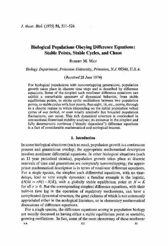
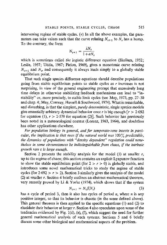
difference equations exhibit a spectrum of dynamical behavior, which, as the intrinsic growth rate r increases, goes from a stable equilibrium point, to stable cyclic oscillations between two population points, to stable cycles with four points, then eight points, and so on, through to a regime which can only be described as “chaotic” (an apt term coined by Li & Yorke, 1974). For any given value of r, in this chaotic regime there are cycles of period, 2, 3, 4, 5, . . . , n, . , , , where n is any positive integer, along with an uncountable number of initial points for which the system does not eventually settle into any finite cycle; whether the system converges on a cycle, and, if so, which cycle, depends on the initial population point (and some of the cycles may be attained only from infinitely unlikely initial points). Figure 1 aims to illustrate this range of behavior.

,:trwl-----1 IO 20 30

Tme (ti

FIG. 1. Spectrum of dynamical behavior of the population density, Nt/K, as a function of time, t, as described by the difference equation (1) for various values of r. Specifically: (a) Y = 14, stable equilibrium point; (b) r = 2.3, stable two-point cycle; (c) r = 2.6, stable four-point cycle; (d), (e), (f) are in the chaotic regime, where the detailed character of the solution depends on the initial population value, with (d) r = 3.3 (N,,/K = 0,075) (e) r = 3.3 (No/K = l-S), (f) r = 5.0 (No/K = O-02).

STABLE POINTS, STABLE CYCLES, CHAOS 513

Specifically, consider the simple nonlinear equation N t + I = Nt exp IN - Nt/QI. (1)

This is considered by some people (Macfadyen, 1963; Cooke, 1965) to be the difference equation analogue of the logistic differential equation, with r and K the usual growth rate and carrying capacity, respectively. The stability character of this equation, as a function of increasing r, is set out in Table 1, and illustrated by Fig. 1.

TABLE] Dynamics of a population described by the dtrerence equation (1)

Dynamical behavior Value of growth rate, r Illustration

Globally stable equilibrium point Globally stable two-point cycle Globally stable four-point cycle Stable cycle, period 8, giving way in turn

to cycles of period 16, 32, etc. as r increases

2>r>O

2.526 > r > 2

2.656 > r > 2-526

2.692 > r > 2.656

Fig. l(a) Fig. l(b) Fig. l(c)

Chaos (cycles of arbitrary period, or aperiodic behavior, depending on initial condition)

r > 2.692 Fig. WI, @I, (0

Another example is

N f + 1 = N,[l + 4 -N,/Io] or, equivalently, defining x = (r/l +r)(N/K),

x~+~ = (l+r)x,(l-x,).

(24

GW In the form (2b), this is probably the simplest nonlinear difference equation one could write down. Although discussed by various people (Maynard Smith, 1968; May, 1972; Krebs, 1972; Scudo & Levine, 1974) as the analogue of the logistic differential equation, equation (2) is less satisfactory than (1) by virtue of its unbiological feature that the population can become negative if at any point Nt exceeds K(1 +r)/r. Thus stability properties here refer to stability within some specific neighborhood, unlike equation (1) where, for example, the stable equilibrium point at N = K is globally stable (for all iV > 0) for 2 > r > 0. With this proviso, the stability behavior of equation (2) is strikingly similar to that of equation (1): see Table 2.

The one-parameter difference equations (1) and (2) are treated in detail to give specificity to the discussion. It is to be emphasized, however, that the

514 R. M. MAY

TABLE 2 Dynamics of a population described by the dyerence equation (2)

Dynamical behavior Value of growth rate, r

Stable equilibrium point 2>r>O Stable two-point cycle 2449 > r > 2 Stable four-point cycle 2-544 > r > 2.449 Stable cycles, period 8, then 16, 32, etc. 2.570 > r > 2.544 Chaos r > 2.570

phenomenon of a threefold regime of a stable point, giving way to stable cycles of period 2”, giving way to chaotic behavior, is a generic one which is liable to occur in any model for discrete generations with the possibility of strongly density-dependent population growth. Some other simple difference equations, which are mainly culled from the entomological literature and which exhibit the phenomenon, are as follows. (i) The equation

N t+1 = A[1 +aNJVbNt

has been used by Hassell (1974) to provide a two-parameter fit to a wide range of field and laboratory data, on single-species population growth: for relatively small values of b or of A there is a globally stable point; the con- junction of moderate values of b and R produces stable cycles; relatively large values of both b.and A leads to chaos. (ii) The density dependent form

N 12 t+1 = a’ ’ l+exp{A(N,-B)} 1 Nt

discussed by Pennycuik, Compton & Beckingham (1968), by Usher (1972), and (in a limiting step-function form) by Williamson (1974), can also exhibit all three regimes as the two parameters A and B are varied. (iii) Similarly the class of models

N ANt t+1 = 1 +(aNJ”

the possible stable points of which have been discussed by Maynard Smith (1974), can show all three types of behavior as A and b vary. (iv) The density dependent equation

N t+1 = lNt [if Nt < B]

N t+i = Y4/WbW [if Nt > B],

discussed by Varley, Gradwell & Hassell (1973), is an interesting example. Here, as a consequence of the pathological discontinuity, the stable point regime (0 < b c 2) gives way directly to the chaotic regime (b > 2), with no

STABLE POINTS, STABLE CYCLES, CHAOS 515

intervening regime of stable cycles. (v) In all the above examples, the para- meters can take values such that the curve relating N,+, to Nt has a hump. To the contrary, the form

N ANt t+1

=---- l+aN,

which is sometimes called the logistic difference equation (Skellam, 1952; Leslie, 1957; Utida, 1967; Pielou, 1969), gives a monotonic curve relating N t+1 and N,, and consequently it always leads simply to a globally stable equilibrium point.

That such single species difference equations should describe populations going from stable equilibrium points to stable cycles as r increases is not surprising, in view of the general engineering precept that excessively long time delays in otherwise stabilizing feedback mechanisms can lead to “in- stability” or, more precisely, to stable limit cycles (see May, 1973, pp. 27-30 and chap. 4; May, Conway, Hassell & Southwood, 1974). What is remarkable, and disturbing, is that the simplest, purely deterministic, single species models give essentially arbitrary dynamical behavior once r is big enough [r > 2.692 for equation (l), r > 2.570 for equation (2)]. Such behavior has previously been noted in a meteorological context (Lorenz, 1963, 1964), and doubtless has other applications elsewhere.

For population biology in general, and for temperate-zone insects in parti- cular, the implication is that even if the natural world was 100 % predictable, the dynamics of populations with “density dependent” regulation could none- theless in some circumstances be indistinguishable from chaos, tf the intrinsic growth rate r is large enough.

Section 2 presents the stability analysis for the model (1) at smaller r, up to the regime of chaos; this section contains an explicit Lyapunov function to show the stable equilibrium point (for 2 > r > 0) is globally stable, and introduces some novel mathematical tricks to study the regime of stable cycles (for 2.692 > P > 2). Section 3 similarly gives the analysis of the model (2) at smaller r. Section 4 briefly outlines an abstract mathematical theorem, very recently proved by Li & Yorke (1974), which shows that if the system

N t+ I = Ntf(N3 has a cycle of period 3, then it also has cycles of period n, where IZ is any positive integer, so that its behavior is chaotic (in the sense defined above). This general theorem is then applied to the specific equations (1) and (2) to elucidate their behavior at larger r. Section 4 also speculates upon some of the tendencies evidenced by Fig. l(d), (e), (f), which suggest the need for further general mathematical analysis of such systems. Sections 5 and 6 briefly discuss some other biological and mathematical aspects of the problem.

516 R. M. MAY

2. Equation (1): Stable Points and Stable Cycles

We begin by quickly recapitulating the standard linearized analysis for stable equilibrium points of difference equations such as (1), (2) or (3), because these general methods underlie the tricks subsequently introduced in the derivation of stable cycles.

We first find the possible equilibrium points, and then study their stability. Using the general form of equation (3), equilibrium points where N,,, = Nt = N* are the solutions of

j-(N*) = 1. (4)

To examine the stability of such an equilibrium point with respect to small perturbations, write Nt = N* +x,, and linearize about the equilibrium point (neglecting initially small quantities of order x”) to get an equation for the population perturbation x, :

Xt+1 = (1 -Ph. (5)

Here, for notational convenience, we have introduced the definition

Neighborhood stability clearly requires 11 -ccl < 1, which leads to the criterion

2>p>o. (7)

More specifically, if 1 > ,u > 0 the perturbations are monotonically damped, and if 2 > p > 1 they are damped in an oscillatory manner.

Applied to equation (l), where f(N) = exp [r(l -N/K)], equation (4) leads to a unique equilibrium point at

N” = K. (8)

Next, equation (6) reduces to p = r, whence the requirement for this equili- brium point to be a stable one is

2>r>O. (9)

More particularly, perturbations are exponentially damped if 1 > r > 0, oscillatorilly damped if 2 > r > 1.

The above constitutes a linearized stability analysis. However, in this instance we can construct a nonlinear Lyapunov function; that is, a function V, with the properties V, 2 0 and AF’, E V,, 1 - V, I 0. Such a function is

v, = (N,--K)‘. (10) This clearly has the property V, 2 0, and for the quantity AV, we have

STABLE POINTS, STABLE CYCLES, CHAOS 517

AK = Wt+, -N,)(N,+ 1 +N,-2K) for which it may be shown that

AV, I 0 [for all Nt > 01, (11) if, and only if, 2 > r > 0. Therefore the linearized stability analysis is a valid characterization of the global, nonlinear stability properties, and the equili- brium point of equation (8) is globally stable for 2 > r > 0. This is a useful, if special, result.

To study what happens when Y > 2 it is helpful to have recourse to the apparently novel trick of expressing N,,, as a function of N,:

N t+2 = NtdNt), (12) where clearly the function g(N) is defined in terms of thef(N) of the general equation (3) by

g(N) = fWftN.fN))~ (13) The analysis outlined three paragraphs above may now be repeated, step by step, using g(N) instead off(N), to seek stable solutions (N,,, = Nt = Nt-2, etc.) of the equation (12). Such solutions will lead to stable two-point cycles of the kind depicted in Fig. l(b).

Applying this trick specifically to equation (l), we have

g(N) = exp [r-(2-s{exp [r(l -:)I + I})]. (14)

Possible equilibrium solutions, N*, follow from

g(N”) = 1, (15) that is,

2 = (N/K)(exp [r(l -N/K)] + 1). (16) By writing

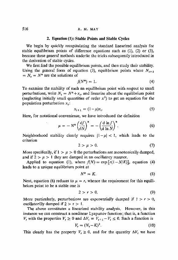
N” E K(l + y), (17) equation (16) may be manipulated into the form

y = tanh (+ry). (18) A graphical way of solving this transcendental equation is indicated in Fig. 2. The essential point is that if r -C 2, there is only one real solution, namely y = O(N* = K), corresponding to the globally stable equilibrium point already discovered for r < 2. However, for r > 2 there are three real solu- tions: the trivial solution y = 0, and a pair of solutions y = +y,-, (with y0 < 1) as indicated in Fig. 2. It may further be shown by the techniques discussed above that the solution y = 0 is always unstable for r > 2, but that each of the pair of solutions N* = K(1 j-yO) is stable provided

2 > r[2-r(l-yg)] > 0. (19) The quantities r and y, are themselves related by equation (1X), whence equation (19) eventually comes down to the constraint r -=c 2.526.

518 R. M. MAY

RG. 2. Graphical solution of equation (18). The straight line depicts the function f(y) = y [the left-hand side of equation (1811; the dashed curve illustrates the function tanh (&+y) if I < 2 (specilkally, r = l), so that the slope near the origin is less than y, and here the only solution of equation (18) is at y = 0; the solid curved line illustrates tanh (+ry) if r > 2 (specifically, r = 4), so that the slope nea.r the origin is greater than y, and here there are necessarily three real solutions of equation (18), at y = 0 and y = i yo.

Thus for r < 2 equation (1) has a stable equilibrium point at N* = K, but as Y increases beyond 2 this solution becomes unstable, and bifurcates into a pair of points N * = K(1 +yO), between which the population alternates _ in a two-point cycle which is stable provided 2 < r c 2.526. Extensive numerical studies suggest this two-point cycle is globally stable for these values of r.

Beyond Y = 2.526, the two-point cycle in turn becomes unstable, and each of the points bifurcates into two further points, giving a stable four-point cycle, as illustrated in Fig. l(c). The details of this process can be elucidated by studying the relationship

N t+4 = Nt WJ cw which follows from the general equations (3) and (12) with

WI = m7SWdN)). (21) For equation (l), h(N) then follows from equation (14), and we can compute the equilibrium solutions and their stability, along the lines laid down above. We find that for r < 2526 the only real solutions of h(N*) = 1 are the three points just discussed. However, for larger r not only are all these points unstable, but there emerge four further real solutions, which lead to a stable four-point cycle for Y < 2.656.

STABLE POINTS, STABLE CYCLES, CHAOS 519

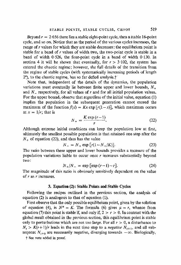
Beyond r = 2.656 there lies a stable eight-point cycle, then a stable 16-point cycle, and so on. Notice that as the period of the various cycles increases, the range of r values for which they are stable decreases : the equilibrium point is stable for a band of r values of width two, the two-point cycle is stable in a band of width 0.526, the four-point cycle in a band of width 0.130. In section 4 it will be shown that eventually, for r > 3.102, the system has entered the chaotic regime; however, the full details of the transition from the regime of stable cycles (with systematically increasing periods of length 2”), to the chaotic regime, has so far defied analysis.7

Note that, independent of the details of the dynamics, the population variations must eventually lie between finite upper and lower bounds, N+ and N- respectively, for all values of r and for all initial population values. For the upper bound5 observe that regardless of the initial value, equation (1) implies the population in the subsequent generation cannot exceed the maximum of the functionf(x) = KX exp [r(l -x)1, which maximum occurs at x = l/r; that is

N +

= K exp (r - 1) r ’ (22)

Although extreme initial conditions can keep the population low at first, ultimately the smallest possible population is that attained one step after the N, of equation (22), and thus has the value

N- = N, exp [r(l-N+/R)]. (23) The ratio between these upper and lower bounds provides a measure of the population variations liable to occur once r increases substantially beyond two :

N+/N- = exp [exp(r-1)-r]. (24) The magnitude of this ratio is obviously sensitively dependent on the value of r as r increases.

3. Equation (2) : Stable Points and Stable Cycles Following the recipes outlined in the previous section, the analysis of

equation (2) is analogous to that of equation (1). First observe that the only possible equilibrium point, given by the solution

of equation (4), is N* = K. The formula (6) gives p = r, whence from equation (7) this point is stable if, and only if, 2 > r > 0. In contrast with the global result obtained in the previous section, this equilibrium point is stable only to perturbations which are not too large. For all r > 0, a disturbance to Nt > K(r+ 1)/r leads in the next time step to a negative Nt+l, and all sub- sequent Nt + k are necessarily negative, diverging towards - co. Biologically,

t See note added in proof.

520 R. M. MAY

of course, such negative values of N imply extinction; but these features of the model (2) make it in some respects less satisfying than (1).

For r > 2, we again turn to study the possibility of stable two-point cycles, using equations (12) and (13) : here g(N) may usefully be written in the form

g(N) = 1 -r31c3(N-K)(N-NA)(N-NB), (25) with the definition

N A,B = (K/2r)[r+2+(r2-4)*]. (26) We see that if r < 2, there is only one real solution of the equation g(N*) = 1, namely the familiar point N* = K. But once r > 2, this solution becomes unstable, and two new solutions of equation (12) split off on either side of it, at N* = NA, NB. These two new points will be stable if equation (7) is satis- fied, where here

r2-4. (27)

Thus equation (2) will have a stable two-point cycle if, and only if,J6 > r > 2, as set out in Table 2.

Again, as r increases beyond & each of these two points bifurcates, to give stable four-point cycles if 2.544 > r > 2449; and so on. As for the previous example, the next section shows that eventually a regime of chaos is established for r > 2.828. Again, the details of the transition zone where stable cycles of period 2” merge into the chaotic regime are not yet elucidated.?

4. Three-point Cycles and Chaotic Behavior

Motivated by earlier work of Lorenz (1963, 1964), published in the meteorological literature, Li & Yorke (1974) have very recently proved an abstract mathematical theorem which is relevant to our present discussion of ecological equations such as (1) and (2). Suppose the general difference equation (3) has a three-point cycle, that is a solution such that Iv,,, = Nt = N*, with N,,, # Nt+2 # N*. It then necessarily follows that there are also cycles with period ~1, where n is any positive integer, and furthermore that there are an uncountable number of initial points NO from which the system does not eventually settle into any of these cycles (that is, is not “asympto- tically periodic”). In these circumstances, whether the system will converge upon one of the cycles, and, if so, which cycle, depends on the starting point, No.

We now apply this general mathematical theorem to the ecologically interesting equations (1) and (2). First we seek a cyclic solution, with period 3,

t See note added in proof.

STABLE POINTS, STABLE CYCLES, CHAOS 521

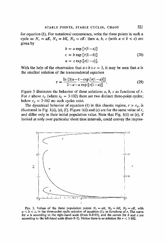
for equation (1). For notational convenience, write the three points in such a cycle as N1 = aK, N2 = bK, N3 = cK: then a, b, c (with a < b < c) are given by

b = a exp [r(l-a)]

c = b exp [r(l- b)] (28)

a = c exp [r(l -c)].

With the help of the observation that a+ b+c = 3, it may be seen that a is the smallest solution of the transcendental equation

In {3/a-l-exp[r(l-a)]} r = 2-a-a exp [r(l-a)] ’ (29)

Figure 3 illustrates the behavior of these solutions a, b, c as functions of r. For r above r, (where rc = 3.102) there are two distinct three-point cycles; below rc = 3.102 no such cycles exist.

The dynamical behavior of equation (1) in this chaotic regime, r > r,-, is illustrated in Fig. l(d), (e), (f). F’g I ure l(d) and (e) are for the same value of r, and differ only in their initial population value. Note that Fig. l(d) or (e), if looked at only over particular short time intervals, could convey the impres-

FlG. 3. Values of the three population points Nl = c%, Nz = bK, Na = cK, with a < b < c, in the three-point cyclic solution of equation (l), as functions of r. The curve for a is according to the right-hand scale (from O-0.03), and the curves for b and c are according to the left-hand scale (from O-3). Notice there is no solution for r < 3-102.

522 R. M. MAY

sion of being locked into a three-point cycle; there is a tendency to be “captured” into almost-periodic three-point cycles, in between episodes of apparently chaotic behavior. A detailed understanding of these properties remains an interesting mathematical problem, related to that of determining what fraction of the totality of initial points converge to a three-point cycle, what fraction to a five-point cycle, and so on, ending with a determination of the fraction of initial points which lead to aperiodic behavior.

For relatively large values of Y beyond rc [e.g., Fig. l(f)], the population fluctuations become more severe, as indicated earlier by the asymptotic upper and lower limits (22) and (23). Notice, however, that the mean popula- tion remains around the value K, as follows from the remark that for equa- tion (1) . ,

>I , that is,

j-l izo j~,+~ = jK[l -(l/rj) ln (N,+j/NJ]*

Thus, for a long time sequence, j % 1, we have

(N) N K. (32) As r becomes large, this mean value is increasingly constituted of a few fairly large population values, together with long sequences of very low population values [e.g., Fig. l(f)]. Very approximately, we may observe from equa- tion (22) that the large fluctuations will have an amplitude around K[exp (r- 1)1/r, and will consequently on the average be spaced (l/r) exp (r- 1) time intervals apart. This gives qualitative insight into the numerical results.

It remains to find the value of r which marks the onset of three-point cycles, and consequent chaos, in equation (2). To this end, we use the form (2b), and seek solutions a < b < c such that

b = (l+r)a(l-a)

c = (l+r)b(l-b). (33) a = (l+r)c(l-c)

Numerical computations reveal that such real solutions can be found if, and only if, r > 2.828. [Li & Yorke (1974) have already remarked, by way of an example, that this difference equation has three-point cycles once r 2 3.1

5. Multispecies Difference Equations

The above discussion is restricted to single species systems obeying differ- ence equations. Similar considerations are likely to apply, a fortiori, to

STABLE POINTS, STABLE CYCLES, CHAOS 523

multispecies situations. Here analytic results are hard to come by; some numerical studies are reported elsewhere (May, 1974a).

6. Discussion

Equations (1) and (2) are two of the simplest nonlinear difference equations to be found. Their rich dynamical structure is a fact of considerable mathe- matical interest, which deserves to be more widely appreciated.

Previous work in this general area of population biology includes, inter ah, remarks on the relation between differential equation models and difference equation models (Van der Vaart, 1973; May, 1972), and on the equivalence between difference equations and differential equations with explicit time-delays (May et al., 1974; Maynard Smith, 1968; McMurtrie, 1974). Earlier discussions of the stability properties of equations (1) and (2) consist of linearized analyses showing the equilibrium point is in both cases only stable for 2 > r > 0 [Cook, 1965 for (1); Maynard Smith, 1968 for (211, with larger r usually dismissed as “unstable, with diverging oscillations”. Very recently, May (1974b) has noted the stable two- and four-point cycles for these equations when r > 2, and Scudo & Levine (1974) have indepen- dently noted the two-point cycle behavior in equation (2).

The transition, as r increases beyond r,-, into a regime of apparent chaos, with cycles of essentially arbitrary period possible, is a result /with many ecological implications. It could be particularly relevant to temperate insect populations, where the natural description is in terms of nonlinear or “density dependent” difference equations, often with relatively large r. In conclusion, it may be emphasized that without an understanding of the range of behavior latent in deterministic difference equations, one could be hard put to make sense of computer simulations or time-series analyses of such models.

I am indebted to R. E. McMurtrie, G. F. Oster, and a reviewer (J. R. Beddington) for helpful comments. I particularly thank 5. A. Yorke for drawing his very elegant work to my attention.

REFERENCES COOK, L. M. (1965). Nature, Lond. 207, 316. H.&SELL, M. P. (1974). J. him. Ecol. (in press). KREBS, J. R. (1972). Ecology: The Experimental Analysis of Distribution and Abundance.

New York: Harper and Row. LESLIE, P. H. (1957). Biometrika 44, 314. LI, T.-Y. & YORKE, J. A. (1974). SIAM J. Math. Anal. (in press). LORENZ, E. N. (1963). J. Amos. Sci. 20,448. LORENZ, E. N. (1964). Tellus 16, 1. MACFADYEN, A. (1963). Animal Ecology. London: Pitman. MCMURTRIE, R. (1974). (In press.)

524 R. M. MAY

MAY, R. M. (1972). Am. Nat. 107, 46. MAY, R. M. (1973). Stability and Complexity in Model Ecosystems. Princeton: Princeton

University Press. MAY, R. M. (19744. Science, N. Y. (in press). MAY, R. M. (19746). In Progress in Theoretical Biology, vol. 3 (R. Rosen & F. Snell, eds).

New York: Academic Press. MAY, R. M., CONWAY, G. R., HA~SELL, M. P. & SOUTHWOOD, T. R. E. (1974). J. Anim.

Ecol. (in press). MAYNARD Sm, J. (1968). Mathematical Ideas in Biology. Cambridge: Cambridge

University Press. MAYNARD SMITH, J. (1974). Models in Ecology, p. 53. Cambridge: Cambridge University

Press. PENNYCUIK, C. J., COMPTON, R. M. & BECKINGHAM, L. (1968). J. theor. Biol. 18, 316. PIELOU. E. C. (1969). An Introduction to Mathematical Ecolonv. New York: Wiley. Scmo; F. M. ‘& L&NE, F. (1974). (In press.)

-_

SKELLAM, J. F. (1952). Biometrika 39, 346. USHER, M. B. (1972). In Mathematical Models in Ecology (J. N. R. Jeffers, ed.), pp. 29-60.

Oxford : Blackwells. USA, S. (1967). Res. Pop. Ecol. 9, 1. VAN DER VAART, H. R. (1973). Bcdl. math. Biophys. 35, 19.5. VARLEY, G. C., GRADWELL, G. R. & HASSELL, M. P. (1973). Insect Population Ecology,

pp. 20-25. Oxford: BIackwells. WILLIAMSON, M. (1974). In Ecological Stability (M. B. Usher & M. Williamson, eds),

pp. 17-34. London: Chapman and Hall.

Note added in proof:

These analytic difficulties have recently been resolved (May & Oster, to be published). Tables 1 and 2 incorporate these latest results, and give an accurate description of the dynamical behavior of equations (1) and (2).