ARTICLE IN PRESS Deep-Sea Research II 51 (2004) 1215–1236 Biomass of Antarctic krill in the Scotia Sea in January/February 2000 and its use in revising an estimate of precautionary yield Roger P. Hewitt a, , Jon Watkins b , Mikio Naganobu c , Viacheslav Sushin d , Andrew S. Brierley b,1 , David Demer a , Svetlana Kasatkina d , Yoshimi Takao e , Cathy Goss b , Alexander Malyshko d , Mark Brandon f , So Kawaguchi c , Volker Siegel g , Philip Trathan b , Jennifer Emery a , Inigo Everson b , Denzil Miller h a Southwest Fisheries Science Center, 8604 La Jolla Shores Drive, La Jolla, CA 92037, USA b British Antarctic Survey, NERC, High Cross, Madingley Road, Cambridge CB3 0ET, UK c National Research Institute of Far Seas Fisheries, Orido 5-7-1, Shimizu, Shizuoka 424, Japan d AtlantNIRO, 5 Dimitry Donskoy Street, Kaliningrad 236000, Russia e National Research Institute of Fisheries Engineering, Ebidai Hasaki, Kashima-gun, Ibaraki 314-0421, Japan f Earth Sciences, The Open University, Milton Keynes MK7-6AA, UK g Institut fu¨r Seefischerei, Palmaille 9, D-22767 Hamburg, Germany h Marine and Coastal Management, Private Bag X2, Roggebaai 8012, South Africa Accepted 18 June 2004 Available online 23 September 2004 Abstract In January and February 2000, a collaborative survey designed to assess the biomass of Antarctic krill across the Scotia Sea was conducted aboard research vessels from Japan, Russia, the UK and the USA using active acoustic and net sampling. Survey design, sampling protocols, and data analysis procedures are described. Mean krill density across the survey area was estimated to be 21.4 g m 2 , and total biomass was estimated to be 44.3 million tonnes (CV 11.4%). This biomass estimate leads to a revised estimate of precautionary yield for krill in the Scotia Sea of 4 million tonnes. However, before the fishery can be permitted to expand to this level, it will be necessary to establish mechanisms to avoid concentration of fishing effort, particularly near colonies of land-breeding krill predators, and to consider the effects of krill immigrating into the region from multiple sources. Published by Elsevier Ltd. www.elsevier.com/locate/dsr2 0967-0645/$ - see front matter Published by Elsevier Ltd. doi:10.1016/j.dsr2.2004.06.011 Corresponding author. E-mail address: [email protected] (R.P. Hewitt). 1 Present address: Getty Marine Laboratory, University of St. Andrews, St. Andrews, Fife, Scotland.
Transcript
ARTICLE IN PRESS
0967-0645/$ - se
doi:10.1016/j.ds
�Correspondi
E-mail addre1Present addr
Deep-Sea Research II 51 (2004) 1215–1236
www.elsevier.com/locate/dsr2
Biomass of Antarctic krill in the Scotia Sea inJanuary/February 2000 and its use in revising
an estimate of precautionary yield
Roger P. Hewitta,�, Jon Watkinsb, Mikio Naganobuc, Viacheslav Sushind,Andrew S. Brierleyb,1, David Demera, Svetlana Kasatkinad, Yoshimi Takaoe,
Cathy Gossb, Alexander Malyshkod, Mark Brandonf, So Kawaguchic,Volker Siegelg, Philip Trathanb, Jennifer Emerya, Inigo Eversonb, Denzil Millerh
aSouthwest Fisheries Science Center, 8604 La Jolla Shores Drive, La Jolla, CA 92037, USAbBritish Antarctic Survey, NERC, High Cross, Madingley Road, Cambridge CB3 0ET, UK
cNational Research Institute of Far Seas Fisheries, Orido 5-7-1, Shimizu, Shizuoka 424, JapandAtlantNIRO, 5 Dimitry Donskoy Street, Kaliningrad 236000, Russia
eNational Research Institute of Fisheries Engineering, Ebidai Hasaki, Kashima-gun, Ibaraki 314-0421, JapanfEarth Sciences, The Open University, Milton Keynes MK7-6AA, UK
gInstitut fur Seefischerei, Palmaille 9, D-22767 Hamburg, GermanyhMarine and Coastal Management, Private Bag X2, Roggebaai 8012, South Africa
Accepted 18 June 2004
Available online 23 September 2004
Abstract
In January and February 2000, a collaborative survey designed to assess the biomass of Antarctic krill across the
Scotia Sea was conducted aboard research vessels from Japan, Russia, the UK and the USA using active acoustic and
net sampling. Survey design, sampling protocols, and data analysis procedures are described. Mean krill density across
the survey area was estimated to be 21.4 g m�2, and total biomass was estimated to be 44.3 million tonnes (CV 11.4%).
This biomass estimate leads to a revised estimate of precautionary yield for krill in the Scotia Sea of 4 million tonnes.
However, before the fishery can be permitted to expand to this level, it will be necessary to establish mechanisms to
avoid concentration of fishing effort, particularly near colonies of land-breeding krill predators, and to consider the
effects of krill immigrating into the region from multiple sources.
R.P. Hewitt et al. / Deep-Sea Research II 51 (2004) 1215–12361216
1. Introduction
The highest concentrations of Antarctic krill(Euphausia superba), krill predators, and krill-fishing effort in the Southern Ocean are located inthe Scotia Sea (Agnew and Nicol, 1996; Laws,1985; Marr, 1962). The international fishery isregulated in accordance with the Convention forthe Conservation of Antarctic Marine LivingResources, which is part of the Antarctic Treatysystem. In principle, the Commission for theConservation of Antarctic Marine Living Re-sources (CCAMLR) has adopted a feedbackapproach to management of the krill fishery, bywhich management measures are adjusted inresponse to ecosystem monitoring (Constable etal., 2000; Hewitt and Linen Low, 2000). However,such a scheme remains to be fully developed. Inthe interim, a complementary approach, whichdefines and implements provisions of Article II2 ofthe Convention in reference to the Scotia Sea krillstock, was adopted in order to set a precautionarycatch limit (Butterworth et al., 1991, 1994).
The approach is to set the proportion (g) ofunexploited population biomass (B0) that can beharvested under defined management criteria. Theallowable catch, referred to as the precautionaryyield (Y ), is thus defined as
Y ¼ gB0: (1)
The risks of exceeding the criteria are evaluatedby comparing statistical distributions of popula-tion biomasses generated from simulated popula-tion trajectories, with and without fishingmortality. Uncertainty is accommodated by usingvalues of abundance, recruitment, growth, andmortality drawn from appropriate statistical dis-tributions. The first criterion is to protect theviability of the harvested population and forAntarctic krill is defined such that the probabilitythat the spawning biomass declines to less than20% of its unexploited median level during any
2Article II of the Convention mandates that fisheries be
managed such that: (a) the size of harvested populations is
sufficient to ensure stable recruitment; (b) ecological relation-
ships between harvested and dependent populations are
maintained; and (c) changes to the marine system that cannot
be reversed over two to three decades are prevented.
one year should be less than 10%. The secondcriterion is to protect the viability of krill predatorpopulations; this is defined such that the medianpopulation level should be at least 75% of theunexploited median population level. The thirdcriterion is to evaluate these risks using populationtrajectories that extend at least 20 years. The valueof the harvest rate, expressed as a proportion ofthe unexploited biomass (g), that meets thesecriteria is accepted as the most precautionary.This value, together with an estimate of B0; is usedto set the precautionary yield for krill.
Two important parameters in this analysis areB0 and its associated variance. These values areused to generate a distribution of populationbiomasses from which an initial biomass is drawnfor each population trajectory. Initially, an esti-mate of krill biomass was generated from acousticdata collected during the first international BIO-MASS experiment (FIBEX)3 in 1981 (Trathan etal., 1992), the only large-scale acoustic survey inthis region prior to 2000. Because exploitation hadhistorically been low relative to the size of thefished resource an estimate of the standing stockwas assumed to approximate B0: Recent reports ofthe Scientific Committee of CCAMLR havequestioned the current relevance of this estimate(e.g. CCAMLR, 1995, Annex 4, para 4.61) andhave recommended a new survey.
The reasons for conducting a new survey wererecognition that: (1) several technical improve-ments had been made in the assessment of krillbiomass using active acoustic methods since theFIBEX survey (Everson et al., 1990; Greene et al.,1991; Hewitt and Demer, 1991); (2) the FIBEXsurvey area was substantially less than the knownhabitat of krill in the Scotia Sea (CCAMLR,1995); and (3) the krill population in the Scotia Seamay not be stable. Recently, published evidencesuggests that krill reproductive success may bedependent on multi-year changes in the physicalenvironment (Brierley et al., 1999; Loeb et al.,
3In the early 1980s, the Scientific Committee for Antarctic
Research (SCAR) established the BIOMASS Program (Biolo-
gical Investigations of Antarctic Systems and Stocks). FIBEX
was a multi-national, multi-ship effort to conduct large-scale
acoustic surveys over large areas of the Southern Ocean. See
also El-Sayed (1994).
ARTICLE IN PRESS
4Harvest statistics for Antarctic krill are maintained by the
CCAMLR Secretariat, P.O. Box 213, North Hobart 7002,
R.P. Hewitt et al. / Deep-Sea Research II 51 (2004) 1215–1236 1217
1997; Naganobu et al., 1999; Nicol et al., 2000;White and Peterson, 1996). During periods ofnorthward excursions of the Southern Boundaryof the Antarctic Circumpolar Current (SBACC),the development of winter sea ice is moreextensive, populations of Salpa thompsoni (apelagic tunicate postulated to be a competitorwith krill for access to the spring phytoplanktonbloom) are displaced offshore, and both krillreproductive output and survival of their larvaeare enhanced. During periods of southwardexcursion of the SBACC, the development ofwinter sea ice is less extensive, salps are moreabundant closer to shore, and krill reproductivesuccess is depressed. These interactions may beconfounded by a warming trend observed in theregion of the Antarctic Peninsula over the last 50years (Vaughan and Doake, 1996). The intentionwas to anchor the estimate of precautionary yieldwith the most recent and accurate assessment ofAntarctic krill in the Scotia Sea possible. Becauseharvest rates continue to be low relative to the sizeof the fished resource, it was again assumed thatan estimate of the current standing stock wasequivalent to B0:
Plans for the survey developed over a period of5 years through a series of working papers,discussions at the meetings of the ScientificCommittee of CCAMLR and its working groups,and more formal workshops (CCAMLR, 1995,Annex 4, paras 4.62–4.67; CCAMLR, 1996,Annex 4, paras 3.72–3.75; CCAMLR, 1997,Annex 4, paras 8.121–8.129; CCAMLR, 1998,Annex 4, paras 9.49–9.90; CCAMLR, 1999,Annex 4, paras 8.1–8.74 and Appendix D).The final survey design and protocols for datacollection were adopted by consensus and aredescribed by Trathan et al. (2001) and Watkinset al. (2004).
The survey was conducted during January andFebruary 2000 using the R./V. Kaiyo Maru
(Japan), the R./V. Atlantida (Russia), the RRSJames Clark Ross (UK), and the R./V. Yuzhmor-
geologiya (a Russian research vessel under charterto the US) (Table 1). A 2-week workshop was heldin May/June 2000 to process the acoustic data andto estimate B0 and its associated variance(CCAMLR, 2000a, Annex 4, Appendix G).
CCAMLR subsequently adopted a revised pre-cautionary catch limit for krill (CCAMLR, 2000b;Hewitt et al., 2002). Much of the informationpresented here is drawn from these reports.
2. Survey design and data collection protocols
The defining physical feature of the Scotia Sea isits southern boundary along the Scotia Ridge,extending from the South Shetland Islands eastand north through the South Orkney Islands, theSouth Sandwich Islands, and South Georgia (Fig.1). This ridge influences the direction and intensityof the ACC. Antarctic krill appear to moveeastward through the Scotia Sea via the ACC,although the relative importance of passive trans-port versus active migration is uncertain. Likelysources of immigrants to the Scotia Sea are theBellingshausen Sea to the west and the WeddellSea to the south. Differences in mitochondrialDNA sequences suggest that krill from theseregions may be genetically distinct (Zane et al.,1998). Within the Scotia Sea, zones of waterconvergence, eddies, and gyres are loci for krillconcentrations (Makarov et al., 1988; Witek et al.,1988). Krill spawn in the vicinity of the SouthShetland and South Orkney Islands. Althoughthey are abundant further to the north and eastnear South Georgia, they do not spawn there ingreat numbers and few larvae are found (Fraser,1936; Siegel, 2000). Consumption of krill through-out the Scotia Sea by baleen whales, crabeater andfur seals, pygoscelid penguins and other seabirds,squid and fish is estimated to be between 16 and 32million tonnes per year (Everson and de la Mare,1996). Although higher in previous years, annualharvests of krill since 1992 have averaged approxi-mately 100,000 tonnes.4 Fishing effort has beenconcentrated near the shelf breaks along the northside of the South Shetland, South Orkney, andSouth Georgia archipelagos (Agnew and Nicol,1996).
R.P. Hewitt et al. / Deep-Sea Research II 51 (2004) 1215–12361218
The survey area extended across the Scotia Seaand included the continental shelves, oceanicregions; the major frontal zones associated withthe ACC, and the principal areas of fishing activity(Fig. 1A). The survey design consisted of sevenstrata (four large-scale strata and three mesoscalestrata, Fig. 1B) with randomly spaced paralleltransects within each stratum (Trathan et al.,2001). The mean density on a transect within astratum, as determined from acoustic sampling ofkrill, was considered to be a representative sampleof the mean density of the stratum (Jolly andHampton, 1990). Each vessel also obtained netsamples and profiles of oceanographic parameterson stations conducted near local apparent noonand mid-night each day of the survey.
All ships collected active acoustic data usingSimrad EK500 echosounders (with firmware ver-sion 5.3, modified to generate 1 ms pulse durationfor 200 kHz) connected to hull-mounted 38, 120,and 200 kHz transceivers. The majority of trans-ceiver settings were specified by the agreed datacollection protocols (Watkins et al., 2004), Table 2
lists important transceiver and transducer specificsfor each ship. Samples of volume backscatteringstrength (SV) were collected every 0.71 m fromeach of the transducer faces to 500 m below thesurface. Pings were fired simultaneously on allfrequencies and the interval between pings was 2 s.Pulse duration for all three frequencies was 1 ms.Data output telegrams from the EK500 echosoun-der were logged using SonarData’s EchoLogsoftware. Although acoustic data were logged onall ships continuously throughout the survey,transect data were only collected between thehours of local apparent sunrise and sunset.Nominal vessel speed was set at 10 kn. SeeWatkins et al. (2004) for additional detailsregarding the acoustic sampling protocols.
Acoustic system calibrations were undertakenbefore and after the survey. Initial calibrationswere conducted in Stromness Bay, South Georgia,final calibrations in Stromness Bay (Atlantida) orAdmiralty Bay, King George Island (James Clark
Ross, Kaiyo Maru, and Yuzhmorgeologiya). Allcalibrations were undertaken using the standard
ARTICLE IN PRESS
Fig. 1. Island groups and bathymetry of the Scotia Sea
(shading indicates 500, 1000 and 3000 m isobaths), reproduced
from Hewitt et al. (2002): (A) Survey strata outlined in black
relative to historical fishing activity (red squares) and major
ocean frontal zones (blue lines; from north to south, the
Subantarctic Front, the Polar Front, the Southern Antarctic
Circumpolar Current Front, and the Southern Boundary of the
Antarctic Circumpolar Current). (B) Survey transects color
coded; green indicates those occupied by the Kaiyo Maru,
yellow Atlantida, blue James Clark Ross, and red Yuzhmorgeo-
logiya. Arrows indicate direction of major currents.
R.P. Hewitt et al. / Deep-Sea Research II 51 (2004) 1215–1236 1219
sphere method (Foote, 1990; Foote et al., 1987).The primary calibration spheres were 38.1 mmdiameter tungsten carbide spheres from the samemanufacturing lot, bored and fitted with mono-filament loops; copper spheres of 60.0, 23.0, and13.7 mm diameter also were used. Temperatureand salinity at the calibration sites were similarand within the range of the major portion of theCCAMLR, 2000 Survey area. In two instances
inclement weather slightly prejudiced the qualityof the results. For the Atlantida the secondcalibration, and for the Kaiyo Maru the firstcalibration, were considered to be the better of thetwo. For the Yuzhmorgeologiya and the James
Clark Ross the mean values of the two calibrationswere used. Calibration specifics for each ship arelisted in Table 3 (see also CCAMLR, 2000a,Annex 4, Appendix G Tables 8–11).
Krill were directly sampled using a RectangularMidwater Trawl with an 8 m2 mouth opening(RMT-8; Baker et al., 1973) near local apparentnoon and mid-night each day. The RMT-8 wasfished obliquely down to 200 m and up to thesurface. Standard lengths and maturity stages weredetermined for every krill if the catch was less than100 animals or a subsample of at least 100 animalsif the catch was larger. See Watkins et al. (2004)and Siegel et al. (2004) for additional detailsregarding net sampling protocols.
3. Data processing methods
Echograms were assembled from the ping-by-ping acoustic data and annotated; during thisprocess some parameters set in the echosoundersduring data collection were adjusted. Prior to thesurvey, historical profiles of seawater temperatureand salinity across the Scotia Sea were examined.Averages, weighted in favour of those depthswhere krill were most often observed, werecalculated and the corresponding sound velocitydetermined as 1449 m s�1. Examination of profilesobtained during the survey indicated that a valueof 1456 m s�1 would be more appropriate.Although this change had a very minor effect,the data were processed using the new value.Absorption coefficients were set to 0.010 dB m�1
for the 38 kHz data, 0.028 dB m�1 for the 120 kHzdata, and 0.041 dB m�1 for the 200 kHz data(Francois and Garrison, 1982). The nominalresonant frequency of the transducers was usedto set the wavelengths at 0.03844 m for the 38 kHzdata, 0.01223 m for the 120 kHz data, and0.00728 m for the 200 kHz data. The equivalenttwo-way beam angle for each transducer, asprovided by the manufacturer for a nominal sound
ARTICLE IN PRESS
Table 2
Ship-specific transducer specifications and transceiver settings during data collection
Transceiver specification/setting Atlantida James Clark Ross Kaiyo Maru Yuzhmorgeologiya
Sphere type 38.1 mm WC 38.1 mm WC 38.1 mm WC 38.1 mm WC 38.1 mm WC 38.1 mm WC
Range to sphere (m) 30.0 38.0 29.2 37.6 29.0 37.6
Calibrated Sv gain (dB) 22.43 22.29 25.37 25.16 26.12 25.80
Selected Sv gain (dB) 22.36 25.26 25.96
Calibrated TS gain (dB) 22.64 22.37 25.56 25.17 26.12 25.80
Selected TS gain (dB) 22.51 25.37 25.96
R.P. Hewitt et al. / Deep-Sea Research II 51 (2004) 1215–12361222
Yuzhmorgeologiya and Atlantida, and 20 m fordata from the James Clark Ross and Kaiyo Maru.Because krill may occur near the surface, evenduring daylight hours, reconstructed echogramswere reviewed and adjustments were made toinclude near-surface biological scatter or toexclude surface noise spikes. This was carried outby a combination of changing the overall depth ofthe surface exclusion layer or editing smallfragments of the surface exclusion layer aroundindividual targets. Table 4 lists surface exclusionlayer depths for each transect by ship. Bottom, asdetected by the echosounder, was visually verifiedfrom the re-constructed echograms and adjusted,if necessary, to ensure that bottom echoes wereexcluded from the integrated layer. The lowervertical limit of integration was set to 500 or 2 mabove the detected bottom where shallower.
No adjustment for noise was made during datacollection (i.e. Noise Margin was set to zero underthe EK500 Operation Menu). During data proces-sing, time-varied volume backscattering strengthdue to noise was estimated and subtracted fromthe echograms (Watkins and Brierley, 1995).Initial estimates of noise were made for eachtransect and frequency during the survey and used
to generate time-varied echograms of noise only.These were visually compared with echogramsmade with the original data using similar valuesfor the absorption coefficients and the displaythresholds for SV: Noise levels were adjusted untilthe effects of noise at long ranges appeared equalon each display; another 2 dB was then added inorder to arrive at a conservative adjustment fornoise. The final values used are listed in Table 4.
Regions of the reconstructed echograms wereattributed to krill when the difference in meanvolume backscattering strength at 120 and 38 kHzwas greater than 2 dB and less than 16 dB(Watkins and Brierley, 2002). Comparisons ofsingle samples of SV were too variable to allowcontiguous regions of the echograms to bedelineated as krill. It was therefore necessary toaverage SV over bins of finite vertical andhorizontal dimension. It was expected that thesize of the bins would necessitate a trade-off. Ifthey were too small, the variability between SV
samples would cause the continuous nature of krillswarms and layers apparent on the echograms tobe lost. If the bins were too large, the power todelineate krill was diminished because backscatterfrom both krill and non-krill scatterers would be
ARTICLE IN PRESS
Table 4
Surface exclusion layer depths and noise levels (dB) for each transect by ship
Ship Transect Surface layer (m) Noise (Sv re 1 m)
38 kHz 120 kHz 200 kHz
Yuz SG01 20 �123.00 �123.00 �123.00
Yuz SG02 20 �124.00 �120.00 �121.00
Yuz SG03 20 �125.00 �124.00 �124.00
Yuz SG04 15 �137.00 �129.00 �124.00
Yuz SS02 20 �137.00 �123.00 �124.00
Yuz SS05 15 �135.00 �125.00 �123.00
Yuz SS08 15 �131.00 �125.00 �123.00
Yuz SOI01 15 �126.00 �120.00 �119.00
Yuz SOI02 15 �126.00 �122.00 �123.00
Yuz SOI03 15 �129.00 �122.00 �122.00
Yuz SOI04 20 �135.00 �127.00 �122.00
Yuz AP11 20 �129.00 �120.00 �123.00
Yuz AP14 15 �129.00 �120.00 �125.00
Yuz AP17 20 �121.00 �120.00 �117.00
Atl Sand01 15 �127.00 �136.50 �135.00
Atl Sand02 15 �127.00 �136.50 �135.00
Atl Sand03 15 �127.00 �136.50 �135.00
Atl Sand04 15 �127.00 �136.50 �135.00
Atl Sand05 15 �127.00 �136.50 �135.00
Atl Sand06 15 �127.00 �136.50 �135.00
Atl Sand07 15 �127.00 �136.50 �135.00
Atl Sand08 15 �127.00 �136.50 �135.00
Atl Sand09 15 �127.00 �136.50 �135.00
Atl Sand10 15 �127.00 �136.50 �135.00
Atl SSa 15 �127.00 �136.50 �135.00
Atl SSb 15 �127.00 �136.50 �135.00
Atl SSc 15 �127.00 �136.50 �135.00
JCR SS01 20 �150.00 �124.00 �110.00
JCR SS04 15 �150.00 �124.00 �112.00
JCR SS07 20 �150.00 �124.00 �112.00
JCR SS10 20 �150.00 �124.00 �110.00
JCR AP13 20 �150.00 �124.00 �110.00
JCR AP16 20 �150.00 �124.00 �110.00
JCR AP19 20 �152.00 �124.00 �110.00
KyM SS03 20 �136.40 �136.40 �134.40
KyM SS06 20 �147.40 �136.40 �138.10
KyM SS09 20 �141.90 �136.80 �138.40
KyM AP12 20 �147.00 �135.70 �135.10
KyM AP15 20 �148.10 �136.20 �136.10
KyM AP18 20 �147.40 �136.60 �136.80
KyM SSI01 20 �140.90 �136.60 �134.40
KyM SSI02 20 �138.90 �136.60 �133.40
KyM SSI03 20 �144.90 �136.60 �133.40
KyM SSI04 20 �141.90 �136.60 �135.40
KyM SSI05 20 �144.90 �136.60 �134.40
KyM SSI06 20 �146.90 �136.60 �135.40
KyM SSI07 20 �149.90 �136.60 �135.40
KyM SSI08 20 �152.90 �136.60 �135.40
Atl—Atlantida; JCR—James Clark Ross; KyM—Kaiyo Maru; Yuz—Yuzhmorgeologiya.
R.P. Hewitt et al. / Deep-Sea Research II 51 (2004) 1215–1236 1223
ARTICLE IN PRESS
R.P. Hewitt et al. / Deep-Sea Research II 51 (2004) 1215–12361224
averaged together. Experimentation with bin sizeon selected echograms indicated little change inintegrated energy attributed to krill when bin sizeis set larger than some minimal dimensions andsmaller than very large regions of the echograms.Bin size was set at 5 m vertical dimension and 50pings horizontal dimension (approximately 500 mat 2 s ping interval and 10 kn survey speed), butcomparable results could have been obtained if thebin size was half or double these dimensions.
Following these procedures, SV samples wereadjusted for changes in assumed values for soundspeed, absorption coefficients, and acoustic wave-lengths; surface exclusion layers were set andadjusted where appropriate; bottom detectionwas verified and modified where appropriate; andreconstructed echograms were annotated to in-clude in subsequent analyses only those datacollected along the designated transects (excludedwere data collected between transects, duringstation times, and within the period between localapparent sunset and local apparent sunrise). Theechograms were then resampled; time-varied noiseechograms were created and subtracted from theresampled echograms; for each transect the 38 kHznoise-free resampled echogram was then sub-tracted from the 120 kHz noise-free resampledechogram; and portions of the 120 kHz noise-freeresampled echogram were masked to excluderegions where the difference between the meanvolume backscattering strength at 120 and 38 kHzwas less than 2 dB or greater than 16 dB. Themasked noise-free resampled 120 kHz echogramwas then integrated from the bottom of the surfaceexclusion layer to 500 m (2 m above the bottom ifshallower than 500 m) and averaged over 1852 m(1 nm) horizontal distance intervals. The outputfrom these analyses was a series of integratedbackscattering areas attributed to krill (sA), onevalue for each nm of acoustic transect, where sA isexpressed in units of m2 of backscattering crosssectional area per square nm of sea surface area orNautical Area Scattering Coefficient (NASC;MacLennan et al., 2002).
Conversion of integrated backscattering areaattributed to krill to areal krill biomass density (r)was accomplished by applying a series of factors(C) equal to the quotient of the weight of an
individual krill (W ðLÞ) and its backscatteringcross-sectional area (sðLÞ) summed over thesampled body length (L) frequency distribution(Hewitt and Demer, 1993):
r ¼ sACg
m2
� �where C ¼
W ðLÞ
sðLÞand L is expressed in mm: ð2Þ
A weight-length relationship was derived fromdata collected aboard the Kaiyo Maru during theCCAMLR, 2000 Survey:
W ðLÞ ¼ 2:236 � 10�6L3:314: (3)
Backscattering cross-sectional area was derivedfrom a definition of krill target strength (TS) as afunction of L at 120 kHz adopted by CCAMLR in1991 (CCAMLR, 1991, Annex 5, Paras 4.24–4.30),such that
Substituting Eqs. (2) and (3) into (1), adjusting forunits and summarizing over length frequencydistribution:
C ¼ 0:2917X
f iðLÞ�0:171 where
Xf i ¼ 1: (5)
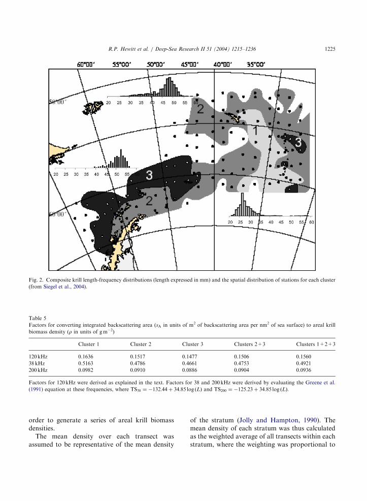
Cluster analysis performed on the net samples ofkrill collected over the CCAMLR, 2000 Surveyarea indicated three geographically distinct regions(Siegel et al., 2004). Small krill (1–2 yr, 26 mmmodal length) were mapped in the eastern ScotiaSea in a broad tongue extending from the southernpart of the survey area between the South Orkneyand South Sandwich Islands north to the easternend of South Georgia; very large krill (4–6 yr,52 mm modal length) were mapped in the westernScotia Sea and Drake Passage; a third cluster oflarge krill (3–5 yr, 48 mm modal length, but alsoincluding several samples of intermediate size krill)was mapped in the inshore waters adjacent to theAntarctic Peninsula and extended across thenortheastern part of the survey area (Fig. 2).Conversion factors for each of these clusters werecalculated and are listed in Table 5. Transects weresubdivided where they crossed cluster boundariesand sA values from sections of the transects in eachcluster were multiplied by the appropriate C in
ARTICLE IN PRESS
Fig. 2. Composite krill length-frequency distributions (length expressed in mm) and the spatial distribution of stations for each cluster
(from Siegel et al., 2004).
Table 5
Factors for converting integrated backscattering area (sA in units of m2 of backscattering area per nm2 of sea surface) to areal krill
Factors for 120 kHz were derived as explained in the text. Factors for 38 and 200 kHz were derived by evaluating the Greene et al.
(1991) equation at these frequencies, where TS38 ¼ �132:44 þ 34:85 log ðLÞ and TS200 ¼ �125:23 þ 34:85 log ðLÞ:
R.P. Hewitt et al. / Deep-Sea Research II 51 (2004) 1215–1236 1225
order to generate a series of areal krill biomassdensities.
The mean density over each transect wasassumed to be representative of the mean density
of the stratum (Jolly and Hampton, 1990). Themean density of each stratum was thus calculatedas the weighted average of all transects within eachstratum, where the weighting was proportional to
ARTICLE IN PRESS
R.P. Hewitt et al. / Deep-Sea Research II 51 (2004) 1215–12361226
the length of each transect:
�rk ¼1
Nk
XNk
j¼1
wj �rj ; (6)
where �rk is the mean areal krill biomass density inthe kth stratum, Nk is the number of transects inthe kth stratum, and wj is the normalized weight-ing factor for the jth transect as defined below, and�rj is the mean areal krill biomass density on the jthtransect as defined below.
For several reasons ships deviated from theplanned transects. Such deviations included ran-dom effects caused by strong winds and oceancurrents, and larger systematic deviations causedby avoidance of icebergs. To correct for theselarger deviations, an expected change in latitudeper nautical mile of transect, DL; was calculatedfor each transect in the survey design. The actuallatitude made good, DL; was derived by differen-cing the latitudes of the beginning and end of eachinterval. An interval weighting W I was calculatedas
W I ¼jDLj � jðDL � DLÞj
DLj j(7)
If the deviation from the standard track line for aparticular interval was greater than 10% (i.e., ifW Io0:9), then the 1 nm integral was scaled byW I ; otherwise W I ¼ 1:
The sum of the interval weightings along eachtransect was used to weight the transect means toprovide a stratum biomass, such that
Lj ¼XNj
i¼1
ðW I Þi; (8)
where Lj is the length of the jth transect, ðW I Þi isthe interval weighting of the ith interval, and Nj isthe number of intervals in the jth transect. Thenormalized weighting factor for the jth transectðwjÞ was defined as
wj ¼Lj
ð1=NkÞSNk
j¼1Lj
such thatXNk
j¼1
wj ¼ Nk: (9)
The mean areal krill biomass density overall intervals on the jth transect ( �rj) was
defined as
�rj ¼1
Lj
XNj
i¼1
ðsAÞiðCÞiðW I Þi; (10)
where ðsAÞi is the integrated backscattering areafor the ith interval and ðCÞi is the conversionfactor for the ith interval. Total biomass over thesurvey area was calculated as
B0 ¼XN
k¼1
Ak �rk; (11)
where Ak is the area of the kth stratum and N isthe number of strata in the survey. Mean densityover the survey area is thus calculated as
�r ¼SN
k¼1Ak �rk
SNk¼1Ak
: (12)
The variance of the mean areal krill biomassdensity in the kth stratum was calculated as a ratioestimator of variance as proposed by Jolly andHampton (1990):
Var �rk
� �¼
Nk
Nk � 1
SNk
j¼1w2j ð �rj � �rkÞ
2
ðSNk
j¼1wjÞ2
¼SNk
j¼1w2j ð �rj � �rkÞ
2
NkðNk � 1Þ: ð13Þ
The contribution of the kth stratum to the overallsurvey variance of B0 was defined as
ðVarðB0Þk ¼ A2K Varð �rkÞ (14)
so that the overall survey variance of the meanareal krill biomass density was calculated as
Varð �rÞ ¼SN
k¼1ðVarðB0ÞÞk
ðSNk¼1AkÞ
2(15)
and the overall survey variance of B0 wascalculated as
VarðB0Þ ¼XN
k¼1
ðVarðB0ÞÞk: (16)
To generate a map of krill dispersion across thesurvey area, estimates of mean areal krill biomassdensity were interpolated onto a grid, of dimen-sions 21 of longitude by 11 of latitude, and thevalues contoured.
ARTICLE IN PRESS
R.P. Hewitt et al. / Deep-Sea Research II 51 (2004) 1215–1236 1227
4. Results
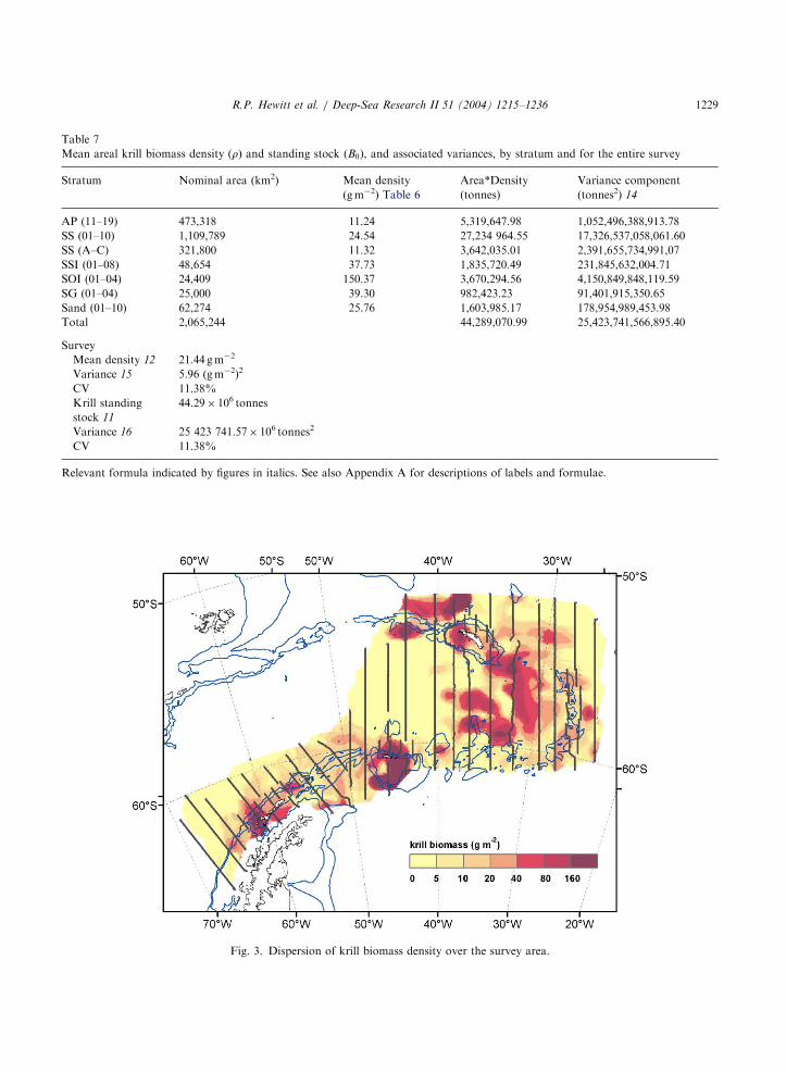
Estimates of areal krill biomass density bytransect, stratum, and survey are listed inTables 6 and 7. Highest densities of krill wereencountered in the mesoscale strata, ranging from25.8 g m�2 (CV 26.4%) near the South SandwichIslands to 150.4 g m�2 (CV 55.5%) near the SouthOrkney Islands; densities in the large-scale strataranged from 11.2 g m�2 (CV 19.3%) off theAntarctic Peninsula to 24.54 g m�2 (CV 15.3%)in the western Scotia Sea; total krill biomass overthe survey area was estimated at 44.3 milliontonnes (CV 11.4%).
Although the densities of krill in the large-scalestrata were generally low, the highest biomass ofkrill was estimated for the large-scale Scotia Seastrata (SS) due to the large area of this stratum(Table 7) coupled with the highest large-scaledensity. However, the highest biomass densitieswere mapped along the Scotia Ridge (Fig. 3), inareas where the fishery has operated in previousyears (Fig. 1A). An area of moderately high krillbiomass density was mapped to the south and eastof South Georgia in water greater than 2000 mdepth. This region coincides with that outlined forthe cluster of small krill (Fig. 2). Approximately,two-thirds of the estimated krill biomass is locatedin areas where fishing has not occurred. Anecdotalevidence suggests that extensive fishing in thelarge-scale strata has not occurred because bio-mass densities are low and/or the location offishable concentrations is not predictable.
There does not appear to be a coherent relation-ship between areas of elevated krill biomassdensity and the position of oceanic fronts (Bran-don et al., 2004). This is consistent with theconclusions of Siegel et al. (2004) with regard tospatial patterns in the demography of krillsampled during the CCAMLR, 2000 Survey. Moreapparent was the association of moderate biomassdensities with high numerical densities of smallkrill (Siegel et al., 2004) in a region with watermass affinities to the Weddell Sea (Brandon et al.,2004). Using flow models Murphy et al. (2004)predicted that these krill were under the pack ice inthe northern Weddell Sea as recently as 2 weeksprior to the survey. Given the cold water intrusion
into the area, the late retreat of sea ice in thevicinity, the identification of Weddell Sea water,and the distinct demographic patterns, Siegel et al.(2004) concluded that the high concentrations ofjuvenile krill in the eastern Scotia Sea were theresult of an intrusion of krill from the south andrepresented a source of krill in the Weddell Seadistinct from the Bellingshausen Sea.
The estimate of B0 and its associated variancederived from the CCAMLR, 2000 Survey wereused to set g at 0.091 (CCAMLR, 2000a, Annex 4,paras 2.96–2.113). The other life history para-meters used in the population simulations arereprinted in Table 8. The precautionary yield (Y )for krill in the Scotia Sea, where gY ¼ B0; was setat 4 million tonnes.
5. Discussion
The estimates of krill biomass and its variancereported here are based on the assumption that thestratified random design proposed by Jolly andHampton (1990) is appropriate. Alternatively, ageostatistical approach (Cressie, 1991) has beenproposed for the design and analysis of acousticsurveys for aquatic organisms (Petitgas, 1993).While the application of geostatistics to acousticsurveys of fish has become widespread, few surveysof zooplankton have incorporated the approach.Murray (1996) compared geostatistical and ran-dom survey analyses as applied to three sets ofacoustic survey data of Antarctic krill collectedduring the 1981 FIBEX survey and averaged overintervals ranging from 0.5 to 11.1 km. The datasetswere highly skewed and little spatial structure wasevident even after separately modeling the upperends of the histograms. The geostatisticallyderived CVs for the data below the truncationpoint were less than that derived from randomsampling theory for the full datasets; however,when combined with the variance estimates for theexcluded portion of the data histogram noimprovement in the CVs was observed. Murray(1996) concluded that the extreme skewness in thekrill data, together with a lack of spatial patternamong the high values, presented problems forthe application of geostatisics. However, Murray
ARTICLE IN PRESS
Table 6
Mean areal krill biomass densities (r) and associated variances by transect and stratum
Total 2,065,244 44,289,070.99 25,423,741,566,895.40
Survey
Mean density 12 21.44 g m�2
Variance 15 5.96 (g m�2)2
CV 11.38%
Krill standing
stock 11
44.29� 106 tonnes
Variance 16 25 423 741.57� 106 tonnes2
CV 11.38%
Relevant formula indicated by figures in italics. See also Appendix A for descriptions of labels and formulae.
Fig. 3. Dispersion of krill biomass density over the survey area.
R.P. Hewitt et al. / Deep-Sea Research II 51 (2004) 1215–1236 1229
ARTICLE IN PRESS
Table 8
Input parameters to the GYM for evaluating g
Category Parameter Estimate
Age structure Recruitment age 0
Plus class accumulation 7
Oldest age in initial structure 7
Recruitment (R) and natural
mortality (M)
M and R dependent on proportion of recruits in stock where:
Proportion of recruits 0.557
Standard deviation of proportion 0.126
Age of recruitment class in proportion 2
Data points to estimate proportion 17
von Bertalanffy growth Time 0 0
L1 60.8 mm
K 0.45
Proportion of year from beginning
in which growth occurs 0.25
Weight at age Weight–length parameter A 1.0
Weight–length parameter B 3.0
Maturity Lm50 32.0–37.0 mm
Range: 0 to full maturity 6 mm
Spawning season 1 December–28 February
Estimate of B0 Survey time 1 February
CV 0.114
Simulation characteristics Number of runs in simulation 1 001
Depletion level 0.2
Seed for random number generator �24189
Characteristics of a trial Years to remove initial age structure 1
Observations to use in median S B0 1 001
Year prior to projection 1
Reference start date in year 1 November
Increments in year 365
Years to project stock in simulation 20
Reasonable upper bound for annual F 5.0
Tolerance for finding F in each year 0.0001
Fishing mortality Length, 50% recruited 30–39 mm
Range over which recruitment occurs 9 mm
Fishing selectivity with age
Fishing season 1 December–1 March
R.P. Hewitt et al. / Deep-Sea Research II 51 (2004) 1215–12361230
(1996) also noted that considering entire transectsas sampling units tended to smooth out smallerscale variations and underestimate the uncertaintyassociated with extremely high values. Geostatis-tical analysis of the data reported here was beyondthe scope of this work but should be considered.
An analysis of the total uncertainty associatedwith the survey was undertaken by Demer (2004)who considered errors associated with systemcalibration, characterization of krill targetstrength, probability of detection, and the effi-ciency of algorithms used to delineate backscatterattributed to krill. Total error was evaluated by
estimating krill biomass for each of the threefrequencies used in the survey, assuming that theidentified errors affect each of these estimatesindependently. Results from a Monte Carlosimulation of this process indicate that the meanof the total error distribution was not significantlydifferent from the estimated sampling variability(i.e., the measurement variance would be negligiblerelative to the sampling variance if averaged overmany surveys). Demer (2004) also consideredpotential biases and concluded that most werenegligible or negative. An exception is speciesdelineation where the algorithm used could not
ARTICLE IN PRESS
R.P. Hewitt et al. / Deep-Sea Research II 51 (2004) 1215–1236 1231
distinguish between small E. superba and othereuphausiids (e.g. Thysanoessa macrura). Morenotable is the disparity observed in krill targetstrength predicted by an empirical model (Greeneet al., 1991) versus a theoretical model (McGeheeet al., 1998). The empirical model, where targetstrength is estimated as a function of body length,is used in the current analyses to convertintegrated volume backscattering strength to krillbiomass density. The theoretical model, wheretarget strength is estimated as a function of bodylength, shape, curvature, orientation angle, andmaterial properties, is impractical to apply undersurvey conditions because so many parametersmust be characterized. One approach is torandomize the sound scattering process by assign-ing appropriate probability density functions tovarious parameter values and estimating a range oftarget strength values for various body lengths(Demer and Conti, 2003). The results of this andsimilar work will be improved estimates of krilltarget strength under natural conditions, whichmay provide a reason for re-evaluating theestimates of krill biomass density reported here.
The latest estimate of B0 and its varianceresulted in revised estimates of g (0.091) and theprecautionary yield of krill (4 million tonnes).Before the fishery can expand to this level,however, it will be necessary to establish mechan-isms to avoid concentration of fishing effort nearcolonies of land-breeding krill predators. In theabsence of detailed information regarding disper-sion and movement of krill throughout theirhabitat, demand by krill predators, and variabilityin recruitment and the factors that control it, anearlier form of the yield model was adopted inorder to establish the original precautionary yield(Butterworth et al., 1991, 1994). The current formof the model (now referred to as the GeneralizedYield Model (GYM; Constable and de la Mare,1996) still assumes a freely distributed krillpopulation, homogeneously distributed predationpressure, and randomly determined recruitment.The effects of uncertainty with regard to inputparameters are included, but spatial and temporaltrends in krill demographics, predator demand,and fishing pressure are not. Several CCAMLRmembers are conducting research studies and long-
term monitoring in order to provide some of thisinformation (Agnew, 1997), but until a morecomplete management scheme is in place theGYM will remain the primary tool for regulatingthe fishery.
One approach to refining the managementscheme is to modify the GYM so as to allowsome of the input parameters to be spatiallyexplicit. In this manner, spatial variations inpredator demand, resulting in spatial variationsin krill mortality, could be incorporated. Similarconsiderations could be made for recruitmentand transport. The GYM would still treat thekrill population in the Scotia Sea as a singlestock, but allowances would be made for varia-bility in population parameters across the region.Results from the CCAMLR, 2000 Survey suggest,however, that krill may be transported into theScotia Sea from two sources (Brandon et al., 2004;Siegel et al., 2004; see also Watkins et al., 1999)and that the assumption of a single stock maybe invalid.
A complementary approach, currently beinginvestigated by CCAMLR, is the establishmentof smaller management units (CCAMLR, 2001,paras 6.15–6.19). Constable and Nicol (2002)suggest that a first step in this approach could beto divide the larger subareas into non-overlappingland-breeding krill predator foraging areas. Thiswas thought to be tractable because the principalarchipelagoes, where breeding colonies of krillpredators are located, are separated by distanceslarger than the predator foraging ranges. Informa-tion regarding predator foraging areas and preydemand would be complemented by informationregarding the immigration and emigration of krillthrough the areas and information on the tacticalbehaviour of the fishery within these areas. Thesedata then could be used to divide the precau-tionary yield among these smaller managementunits more rationally.
The establishment of smaller management unitsas a method for dispersing the harvest alsoassumes the existence of a single stock. However,monitoring within the units would allow forinformation feedback, and consequent adjust-ments to allocation of yield among the units aswell as better characterization of input parameters
ARTICLE IN PRESS
R.P. Hewitt et al. / Deep-Sea Research II 51 (2004) 1215–12361232
to the population model. Identification andmonitoring of key processes regulating the krill-centric ecosystem (Hewitt and Linen Low, 2000)would thus contribute to both the interim and thelong-term goals of CCAMLR. Smaller manage-ment units may also be used in an experimentalfashion. For example, certain units could be closedto fishing while the fishing level in other units maybe allowed to approach g (Constable and Nicol,2002). Suitable monitoring schemes could beestablished to provide the data necessary to testkey assumptions and predictions.
In the meantime, the GYM provides a methodby which uncertainty in population parameterestimates can be explicitly incorporated intoestimates of harvest rate. The framework is flexibleand can accommodate restatement of managementobjectives and reformulation of the criteria used toensure that the objectives are met. While thecurrent criteria may be perceived as somewhatarbitrary they can be refined as new information isacquired regarding the relationships between krillpopulation biomass, recruitment, and predatorresponse. In addition, application of the GYMallows separation of the political process of settingmanagement objectives and criteria from thetechnical process of operating the model and
determining the harvest rate. However, use of theGYM to manage the krill fishery was adopted byCCAMLR as an interim measure to its preferredapproach; that is, a feedback scheme wherebymanagement measures are adjusted in response toecosystem monitoring. The full development ofthis approach will require: (1) enhancement of theexisting CCAMLR ecosystem monitoring pro-gram; (2) high-resolution, real-time informationregarding the activities of fishing vessels; and (3)further development of models linking krill, theirpredators, environmental influences, and thefishery.
6. Deposition of data
Copies of all data files, including raw ping-by-ping echosounder output telegrams (EK5 files),echogram annotation files (EV files), variousintegration output files (CSV files), and summarytables (MS Excel files), are maintained at theCCAMLR Secretariat in Hobart, Australia. SeeRules for Access and Use of CCAMLR Data
available at: www.ccamlr.org.
Appendix A
Descriptors for labels in Tables 6 and 7, where i is used to index intervals along a transect, j is used toindex transects within a stratum, and k is used to index strata.
Transect label
Formula/descriptor
Length
Transect length defined as the sum of all interval weightings
Lj ¼XNj
i¼1
ðW I Þi
where Lj is the length of the jth transect, ðW I Þi is the interval weighting of theith interval, and Nj is the number of intervals in the jth transect.
R.P. Hewitt et al. / Deep-Sea Research II 51 (2004) 1215–1236 1233
such thatPNk
j¼1
wj ¼ Nk where wj is the weighting factor for the jth transect,
and Nk is the number of transects in a stratum.
Krill density measured Mean areal krill biomass density over all intervals on each transect
�rj ¼1
Lj
XNj
i¼1
ðsAÞiðCÞiðW I Þi
where �rj is the mean areal krill biomass density on the jth transect, ðsAÞi is theintegrated backscattering area for the ith interval and ðCÞi is the conversionfactor for the ith interval.
Krill density weighted
Mean areal krill biomass density times the weighting factor �rW j¼ wj �rj
where �rW jis the mean weighted areal krill biomass density on the jth
transect.
Variance component
VarCompj ¼ w2j ð �rj � �rkÞ
2
here VarCompj is the weighted contribution of the jth transect to the stratumvariance.
Stratum label
Formula/descriptor
Mean
Stratum mean areal krill biomass density
�rk ¼1
Nk
XNk
j¼1
wj �rj
where �rk is the mean areal krill biomass density in the kth stratum (afterEq. (1), Jolly and Hampton, 1990).
Variance
Stratum variance
Varð �rkÞ ¼Nk
Nk � 1
PNk
j¼1
w2j ð �rj � �rkÞ
2
PNk
j¼1
wj
!2¼
PNk
j¼1
w2j ð �rj � �rkÞ
2
NkðNk � 1Þ
where Varð �rK Þ is the variance of the mean areal krill biomass density in thekth stratum.
CV (%)
Coefficient of variation
CVk ¼ 100ðVarð �rkÞÞ
0:5
�rk
where CVk is the coefficient of variation for the kth stratum.
Nominal area Area of kth stratum (Ak) estimated at the time of survey design. Mean density Mean areal krill biomass density of the kth stratum, �rk:
ARTICLE IN PRESS
Appendix A (continued)
Stratum label Formula/descriptor
R.P. Hewitt et al. / Deep-Sea Research II 51 (2004) 1215–12361234
Area*density
Ak �rk
Variance component
ðVarðB0ÞÞk ¼ A2
kVarð �rkÞ
where ðVarðB0ÞÞk is the contribution of the kth stratum to the overall surveyvariance of B0:
Survey label
Formula/descriptor
Mean density
Overall survey mean areal krill biomass density
�r ¼
PNk¼1
Ak �rk
PNk¼1
Ak
where N is the number of survey strata (after Eq. (2), Jolly and Hampton,1990).
Variance
Overall survey variance of the mean areal krill biomass density
Varð �rÞ ¼
PNk¼1
A2kVarð �rkÞ
PNk¼1
Ak
2¼
PNk¼1
ðVarðB0ÞÞk
PNk¼1
Ak
2
(after Eq. (3), Jolly and Hampton, 1990).
CV Overall coefficient of variation of the mean areal krill biomass density
CV �r ¼ 100ðVarð �rÞÞ0:5
�r
PN
Krill Standing Stock B0 ¼
k¼1
Ak �rk
Variance
Overall survey variance of B0
VarðB0Þ ¼PNk¼1
ðVarðB0ÞÞk
CV
Overall coefficient of variation of B0
ðVarðB0ÞÞ0:5
CVB0¼ 100
B0
References
Agnew, D.J., 1997. Review: The CCAMLR ecosystem mon-