149
UNIVERSITÀ DEGLI STUDI DI PADOVA
DIPARTIMENTO DI INGEGNERIA INDUSTRIALE
(ex DM 270/2004)
BIOMECHANICAL ANALYSIS OF THESIDESTEP CUTTING MANEUVER INFOOTBALL PLAYERS WITH OPENSIM
Relatori: Prof. Nicola Petrone
Prof. Josep Maria Font Llagunes
Dott. Ventura Ferrer Roca
Laureando: Dennis Da Corte
Matricola: 1036513
ANNO ACCADEMICO 2013/2014


Biomechanical analysis of the sidestep cutting maneuver in football players with OpenSim 1
Abstract
The use of mechanical vibrations has become a very common technique in the training of ath-
letes. Some studies highlight that this kind of training is able to increase the force of the muscles,
but is seems to decrease the capacity of controlling the movements by the subject. This aspect
could increase the risk of ACL injuries.
The aim of this project is to develop a computational model to analyze how a warming up
with mechanical vibrations can affect the biomechanical behavior of the lower limbs, with a
particular attention to the aspects related to the noncontact ACL injuries. For this purpose, a
lower limb model is implemented using the OpenSim software (Stanford University) to obtain
the evolution of joint angles, joint torques and muscle forces during a sidestep cutting maneuver
(before and after warming up). Those results are obtained by means of multibody dynamics
and optimization techniques.
The work also includes an economic study and an analysis of the social and environmental
impact.

2 Final Degree Project - Dennis Da Corte

Biomechanical analysis of the sidestep cutting maneuver in football players with OpenSim 3
Contents
1 Introduction 7
2 Anatomy of the lower limb 9
2.1 Knee joint behavior . . . . . . . . . . . . . . . . . . . . . . . . . . . . . . . . . . . 9
2.1.1 Introduction . . . . . . . . . . . . . . . . . . . . . . . . . . . . . . . . . . 9
2.1.2 Bones . . . . . . . . . . . . . . . . . . . . . . . . . . . . . . . . . . . . . . 10
2.2 Anatomy and phisiology of the skeletal muscle . . . . . . . . . . . . . . . . . . . 14
2.2.1 Introduction . . . . . . . . . . . . . . . . . . . . . . . . . . . . . . . . . . 14
2.2.2 Actions of the skeletal muscles . . . . . . . . . . . . . . . . . . . . . . . . 15
2.2.3 Macroscopic structure of the skeletal muscle . . . . . . . . . . . . . . . . . 15
2.2.4 Architecture of the skeletal muscle . . . . . . . . . . . . . . . . . . . . . . 16
2.2.5 Microstructure of the skeletal muscle . . . . . . . . . . . . . . . . . . . . . 19
2.2.6 Activation of the skeletal muscle . . . . . . . . . . . . . . . . . . . . . . . 20
2.3 Ligaments . . . . . . . . . . . . . . . . . . . . . . . . . . . . . . . . . . . . . . . . 21
3 State of the art 25
3.1 Mechanism of ACL non contact injuries . . . . . . . . . . . . . . . . . . . . . . . 25
4 Experimental methodology 29
4.1 Instrumentation . . . . . . . . . . . . . . . . . . . . . . . . . . . . . . . . . . . . . 29
4.1.1 Motion capture system . . . . . . . . . . . . . . . . . . . . . . . . . . . . . 29
4.1.2 Force platform . . . . . . . . . . . . . . . . . . . . . . . . . . . . . . . . . 35
4.1.3 Electromyography . . . . . . . . . . . . . . . . . . . . . . . . . . . . . . . 36
4.1.4 Mechanical vibrations machine . . . . . . . . . . . . . . . . . . . . . . . . 39
4.2 Execution of the test . . . . . . . . . . . . . . . . . . . . . . . . . . . . . . . . . . 40
4.2.1 Preparation of the tester . . . . . . . . . . . . . . . . . . . . . . . . . . . . 40

4 Final Degree Project - Dennis Da Corte
4.2.2 Protocol of execution of the tests . . . . . . . . . . . . . . . . . . . . . . . 45
5 Numerical methodology 49
5.1 Presentation of OpenSim . . . . . . . . . . . . . . . . . . . . . . . . . . . . . . . 49
5.1.1 Capabilities of OpenSim . . . . . . . . . . . . . . . . . . . . . . . . . . . . 49
5.1.2 How OpenSim works . . . . . . . . . . . . . . . . . . . . . . . . . . . . . . 50
5.2 Procedure of the numerical simulation . . . . . . . . . . . . . . . . . . . . . . . . 50
5.2.1 Preparation of the data . . . . . . . . . . . . . . . . . . . . . . . . . . . . 50
5.2.2 Model . . . . . . . . . . . . . . . . . . . . . . . . . . . . . . . . . . . . . . 53
5.2.3 Scaling tool . . . . . . . . . . . . . . . . . . . . . . . . . . . . . . . . . . . 56
5.2.4 Inverse Kinematics . . . . . . . . . . . . . . . . . . . . . . . . . . . . . . . 58
5.2.5 Inverse Dynamics . . . . . . . . . . . . . . . . . . . . . . . . . . . . . . . . 60
5.2.6 Static Optimization . . . . . . . . . . . . . . . . . . . . . . . . . . . . . . 62
6 Experimental results and discussion 71
6.1 Ground reaction forces . . . . . . . . . . . . . . . . . . . . . . . . . . . . . . . . . 72
6.2 Kinematics . . . . . . . . . . . . . . . . . . . . . . . . . . . . . . . . . . . . . . . 75
6.2.1 Time of duration of the cycle . . . . . . . . . . . . . . . . . . . . . . . . . 76
6.2.2 Load rising rate . . . . . . . . . . . . . . . . . . . . . . . . . . . . . . . . . 77
6.3 EMG . . . . . . . . . . . . . . . . . . . . . . . . . . . . . . . . . . . . . . . . . . . 79
6.4 Conclusions . . . . . . . . . . . . . . . . . . . . . . . . . . . . . . . . . . . . . . . 80
7 Numerical results and discussion 81
7.1 Kinematics . . . . . . . . . . . . . . . . . . . . . . . . . . . . . . . . . . . . . . . 81
7.1.1 Maximum knee flexion angle . . . . . . . . . . . . . . . . . . . . . . . . . 82
7.1.2 Range of motion of the knee flexion . . . . . . . . . . . . . . . . . . . . . 84
7.1.3 Maximum knee abduction angle . . . . . . . . . . . . . . . . . . . . . . . 85
7.1.4 Conclusions . . . . . . . . . . . . . . . . . . . . . . . . . . . . . . . . . . . 88
7.2 Dynamics . . . . . . . . . . . . . . . . . . . . . . . . . . . . . . . . . . . . . . . . 89
7.2.1 Minimum negative knee flexion moment . . . . . . . . . . . . . . . . . . . 90
7.2.2 Minimum negative knee adduction moment . . . . . . . . . . . . . . . . . 93
7.2.3 Range of the moment of flexion of the ankle . . . . . . . . . . . . . . . . . 95
7.2.4 Conclusions . . . . . . . . . . . . . . . . . . . . . . . . . . . . . . . . . . . 97
7.3 Muscular activations . . . . . . . . . . . . . . . . . . . . . . . . . . . . . . . . . . 98

Biomechanical analysis of the sidestep cutting maneuver in football players with OpenSim 5
8 Economic and environmental aspects 113
8.1 Economic cost of the project . . . . . . . . . . . . . . . . . . . . . . . . . . . . . 113
8.2 Environmental impact of the project . . . . . . . . . . . . . . . . . . . . . . . . . 116
8.3 Aspects related to the social cost of ACL injuries . . . . . . . . . . . . . . . . . . 116
9 Conclusions and recommendations 119
10 Appendix 123
10.1 Model parameters . . . . . . . . . . . . . . . . . . . . . . . . . . . . . . . . . . . 123
10.2 Scaling parameters . . . . . . . . . . . . . . . . . . . . . . . . . . . . . . . . . . . 134
10.3 Inverse Kinematics parameters . . . . . . . . . . . . . . . . . . . . . . . . . . . . 137
10.4 Inverse Dynamics parameters . . . . . . . . . . . . . . . . . . . . . . . . . . . . . 138
10.5 Static Optimization parameters . . . . . . . . . . . . . . . . . . . . . . . . . . . . 140
Bibliography 143
11 Ringraziamenti 147

6 Final Degree Project - Dennis Da Corte

Biomechanical analysis of the sidestep cutting maneuver in football players with OpenSim 7
Chapter 1
Introduction
The ACL injury is a very common problem in sports like football, alpine skiing, basketball,
handball, rugby, etc., that just in the United States affects more than 100000 people each year.
This kind of injury requires a very long convalescence, in some cases longer than 6 months.
In this prospective the sports trainers are trying to work in order to find strategies of training
designed to reduce the risk of occurrence of ACL injuries. However, on the other hand, they
design the trainings in order to increase the performances of the athletes. Could these two aims
be at odds with each other?
Some studies on the full body mechanical vibrations warming up highlight that this kind
of training seems to increase the muscular performance of the athletes but, on the other hand,
to decrease the capacity of control and of perception of the knee, bringing to an increase of
possibilities to develop an ACL injury.
The aim of the project is to develop a three-dimensional lower limb multibody model to
investigate the biomechanical effects related to the loss of control of the knee after a mechanical
vibrations warming up. The model, that has a total of 36 degrees of freedom, consists of 6
segments and is actuated by 43 muscles. This project is done in the framework of a collaborative
work among the Biomechanics Division of CREB-UPC at ETSEIB, the CAR of Sant Cugat and
the University of Lleida.

8 Final Degree Project - Dennis Da Corte

Biomechanical analysis of the sidestep cutting maneuver in football players with OpenSim 9
Chapter 2
Anatomy of the lower limb
2.1 Knee joint behavior
2.1.1 Introduction
The knee can be considered as a double condylar articulation together with a trochlea. The lower
limb can be divided mainly in two parts: the thigh and the shank. The first one is situated
between the hip joint and the knee joint and it’s coincident with the femur, the second one is
situated between the knee joint and the ankle joint and it’s coincident with the tibia and the
fibula.
The biomechanical analysis of this joint highlights a principal degree of freedom (DOF) of
flexion. The internal rotation and the adduction have a very low range of motion and they are
often neglected in the mechanical models; anyway the amplitude of these two degrees of freedom
is considered as a good factor to see if there is any problem on the ligaments that constrain the
joint motion.
All the degrees of freedom of the knee joint are shown in Figure 2.1. The range of motion of
the knee reported in literature is the following:
• Flexion: from 0◦ to 120◦;
• Adduction: more or less from -10◦ to +10◦;
• Internal rotation: more or less from -15◦ to 13◦ [11].

10 Final Degree Project - Dennis Da Corte
Figure 2.1: Degrees of freedom of the knee. On the left flexion, on the center adduction, on the right
internal rotation.
2.1.2 Bones
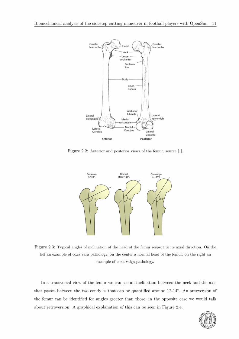
Femur:
The femur, represented in Figure 2.2, is the longest, heaviest and by most measures the
strongest bone in the human body. Its length is 26% of the person’s height, a ratio that is useful
in anthropology because it offers a basis for a reasonable estimate of a subject’s height from an
incomplete skeleton.
The femur comprises a diaphysis (or shaft) and two epiphysis or extremities that articulate
with adjacent bones in the hip and knee. In the proximal extremity of this bone there is a big
protrusion called neck of the femur with a semi-spherical part called head of the femur that
articulates with the acetabulum of the pelvis. There are also two smaller protrusions called
greater and lesser trochanter, which are lever arms for some important muscles.
In a frontal plane, a normal neck of the femur has an inclination of more or less 125-130◦
with respect to the axis of the shaft; an inclination lower than 120◦ is considered as coxa vara,
an inclination higher than 135◦ is considered as coxa valga, two pathologies that influence the
posture of the whole body. A graphical explanation of this can be seen in Figure 2.3.
Biomechanical analysis of the sidestep cutting maneuver in football players with OpenSim 11
Figure 2.2: Anterior and posterior views of the femur, source [1].
Figure 2.3: Typical angles of inclination of the head of the femur respect to its axial direction. On the
left an example of coxa vara pathology, on the center a normal head of the femur, on the right an
example of coxa valga pathology.
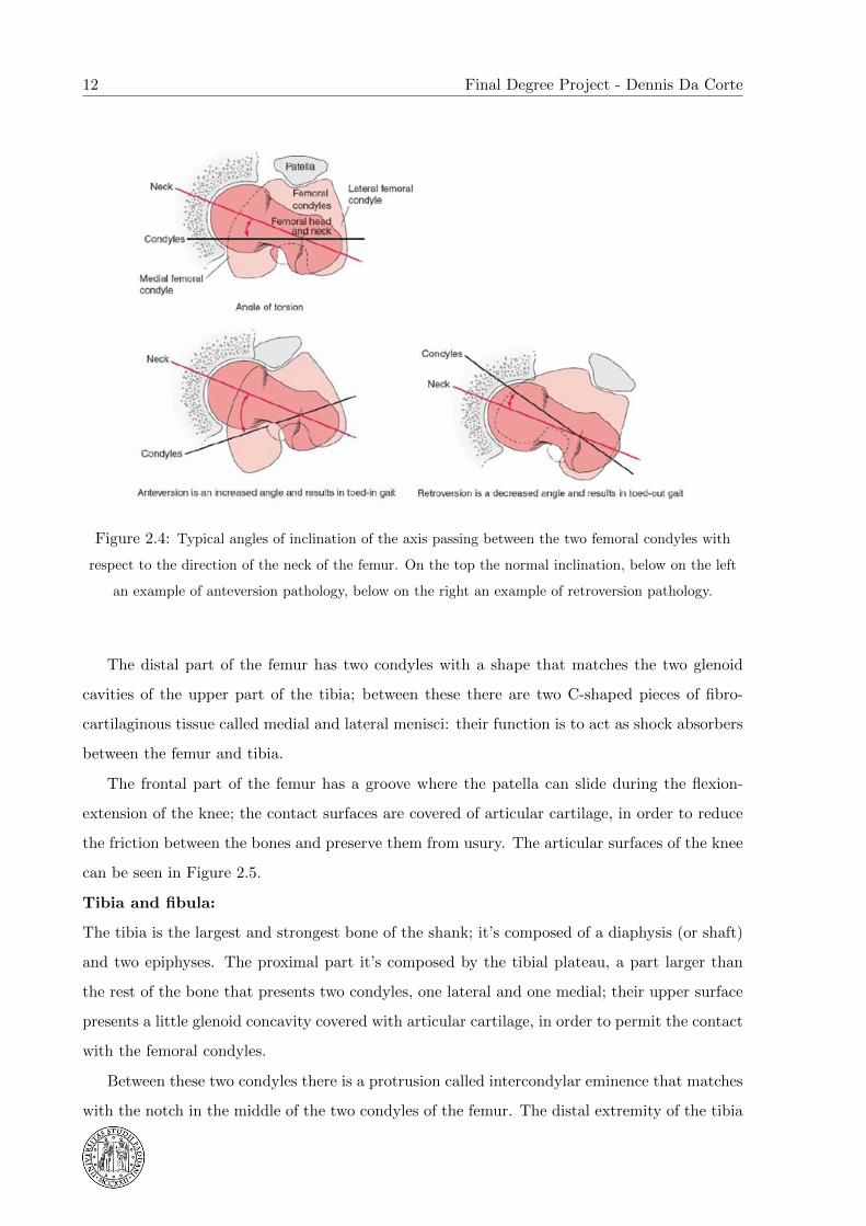
In a transversal view of the femur we can see an inclination between the neck and the axis
that passes between the two condyles that can be quantified around 12-14◦. An anteversion of
the femur can be identified for angles greater than those, in the opposite case we would talk
about retroversion. A graphical explanation of this can be seen in Figure 2.4.
12 Final Degree Project - Dennis Da Corte
Figure 2.4: Typical angles of inclination of the axis passing between the two femoral condyles with
respect to the direction of the neck of the femur. On the top the normal inclination, below on the left
an example of anteversion pathology, below on the right an example of retroversion pathology.
The distal part of the femur has two condyles with a shape that matches the two glenoid
cavities of the upper part of the tibia; between these there are two C-shaped pieces of fibro-
cartilaginous tissue called medial and lateral menisci: their function is to act as shock absorbers
between the femur and tibia.
The frontal part of the femur has a groove where the patella can slide during the flexion-
extension of the knee; the contact surfaces are covered of articular cartilage, in order to reduce
the friction between the bones and preserve them from usury. The articular surfaces of the knee
can be seen in Figure 2.5.
Tibia and fibula:
The tibia is the largest and strongest bone of the shank; it’s composed of a diaphysis (or shaft)
and two epiphyses. The proximal part it’s composed by the tibial plateau, a part larger than
the rest of the bone that presents two condyles, one lateral and one medial; their upper surface
presents a little glenoid concavity covered with articular cartilage, in order to permit the contact
with the femoral condyles.
Between these two condyles there is a protrusion called intercondylar eminence that matches
with the notch in the middle of the two condyles of the femur. The distal extremity of the tibia

Biomechanical analysis of the sidestep cutting maneuver in football players with OpenSim 13
Figure 2.5: Surfaces of the knee and the two menisci, adapted from [15] .
presents a concave articular surface that develops in the medial part in the medial malleolus.
The fibula is the other bone part of the shank. It’s very thin and it’s situated in the lateral
part of the tibia. It’s composed of a diaphysis and two epiphyses. The proximal one has a planar
articular facet, the contact part with the tibia; the distal part becomes the lateral malleolus.
An anterior and posterior view of the tibia and the fibula bones can be seen in Figure 2.6.
Figure 2.6: Anterior and posterior views of the tibia and the fibula.

14 Final Degree Project - Dennis Da Corte
Patella:
The patella, as we can see in Figure 2.7, is a flat, circular-triangular bone which articulates
with the femur and covers and protects the anterior articular surface of the knee joint. It is the
largest sesamoid bone in the human body. Its thickness can be considered as included in the
thickness of the tendon of insertion of the quadriceps muscle. The patella has a very important
role in the extension of the knee and its main importance is in the increasing of the lever arm
of the quadriceps muscle.
Figure 2.7: Anterior and posterior views of the patella, source [16].
2.2 Anatomy and phisiology of the skeletal muscle
2.2.1 Introduction
The muscle tissue is a fundamental part of the human structure. According with the different
structures, functionalities and mechanism of control, we can divide it in three main categories:
the skeletal muscle tissue, the cardiac muscle tissue and the smooth muscle tissue.
• Skeletal muscle tissue: as its name suggests, most skeletal muscles are attached to bones
by bundles of collagen fibers known as tendons. This tissue is striated and is controlled
by the somatic nervous system, so it can be activated voluntarily;
• Cardiac muscle tissue: this tissue is striated and composes the heart; its control is invol-
untary;
• Smooth muscle tissue: this tissue is not striated and composes most of the structure of
the digestive system; its control is involuntary.
Biomechanical analysis of the sidestep cutting maneuver in football players with OpenSim 15
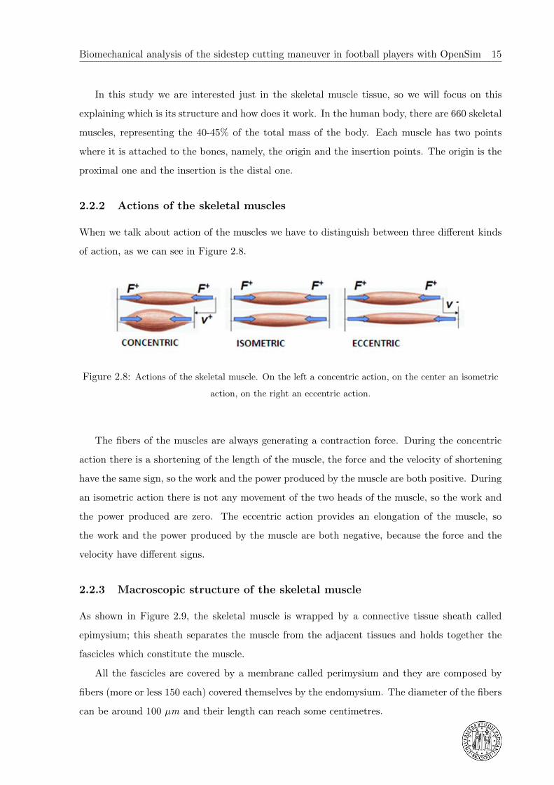
In this study we are interested just in the skeletal muscle tissue, so we will focus on this
explaining which is its structure and how does it work. In the human body, there are 660 skeletal
muscles, representing the 40-45% of the total mass of the body. Each muscle has two points
where it is attached to the bones, namely, the origin and the insertion points. The origin is the
proximal one and the insertion is the distal one.
2.2.2 Actions of the skeletal muscles
When we talk about action of the muscles we have to distinguish between three different kinds
of action, as we can see in Figure 2.8.
Figure 2.8: Actions of the skeletal muscle. On the left a concentric action, on the center an isometric
action, on the right an eccentric action.
The fibers of the muscles are always generating a contraction force. During the concentric
action there is a shortening of the length of the muscle, the force and the velocity of shortening
have the same sign, so the work and the power produced by the muscle are both positive. During
an isometric action there is not any movement of the two heads of the muscle, so the work and
the power produced are zero. The eccentric action provides an elongation of the muscle, so
the work and the power produced by the muscle are both negative, because the force and the
velocity have different signs.
2.2.3 Macroscopic structure of the skeletal muscle
As shown in Figure 2.9, the skeletal muscle is wrapped by a connective tissue sheath called
epimysium; this sheath separates the muscle from the adjacent tissues and holds together the
fascicles which constitute the muscle.
All the fascicles are covered by a membrane called perimysium and they are composed by
fibers (more or less 150 each) covered themselves by the endomysium. The diameter of the fibers
can be around 100 µm and their length can reach some centimetres.

16 Final Degree Project - Dennis Da Corte
Figure 2.9: Macroscopic structure of the skeletal muscle.
2.2.4 Architecture of the skeletal muscle
We can distinguish between different kinds of architecture depending on the disposal of the
fibers respect to the direction of the line connecting the origin and the insertion of the muscle;
we describe the inclination of the fibers respect to the line of action of the muscle with the angle
of pennation (α) as we can see in Figure 2.10.
Figure 2.10: Definition of angle of pennation (α), source [3].
In this way we can distinguish between fusiform muscles and pennate muscles; the latter can
be divided in different categories, according with the number of different directions in which the

Biomechanical analysis of the sidestep cutting maneuver in football players with OpenSim 17
fibers are oriented. The classification of the skeletal muscles respect to this criterion can be seen
in Figure 2.11.
Figure 2.11: Classification of the skeletal muscles according with the macroscopic disposition of the
fibers respect to the line of action of the tendon.
According with the definitions shown in Figure 2.12, it is possible to introduce an index
called “index of architecture” (ia) in order to give an idea of the kind of architecture of the
muscle, considering the ratio between the length of the fibers (lf ) and the length of the muscle
(lm) in a particular optimal condition (Eq. 2.1).
Figure 2.12: Schematization of a pennate muscle.
ia =lflm
(2.1)
Obviously for a fusiform muscle the index of architecture is 1, because the angle of pennation
is zero, so the length of the fibers coincides with the length of the muscle.
18 Final Degree Project - Dennis Da Corte
Every muscle has a parameter that describes which is the nominal strength of the muscle σ0,
the maximum isometric tension that can be generated by the fibers along their direction. The
relationship between strength and force for the muscle has to pass through the definition of two
geometrical parameters:
• Physiological Cross Section Area:
PCSA =V ol
lf(2.2)
• Cross Section Area:
CSA =V ol
lm(2.3)
where “V ol” si the volume of the muscle.
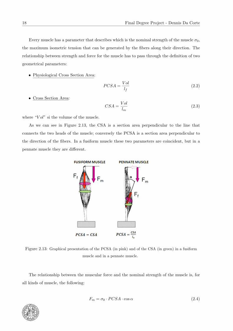
As we can see in Figure 2.13, the CSA is a section area perpendicular to the line that
connects the two heads of the muscle; conversely the PCSA is a section area perpendicular to
the direction of the fibers. In a fusiform muscle these two parameters are coincident, but in a
pennate muscle they are different.
Figure 2.13: Graphical presentation of the PCSA (in pink) and of the CSA (in green) in a fusiform
muscle and in a pennate muscle.
The relationship between the muscular force and the nominal strength of the muscle is, for
all kinds of muscle, the following:
Fm = σ0 · PCSA · cosα (2.4)

Biomechanical analysis of the sidestep cutting maneuver in football players with OpenSim 19
2.2.5 Microstructure of the skeletal muscle
We can have an idea of the miscro structure of the skeletal muscle in Figure 2.14.
Figure 2.14: Micro structure of the skeletal muscle, source [8].
The smallest component of the macroscopic structure of the muscle is the muscle fiber with
a diameter around 100 µm. The fiber is composed by a lot of filaments called myofibrils.
Each myofibril is divided in different portions by transversal lines; in the portion between two
contiguous Z lines we can identify the sarcomere, the elementary structure of the muscle. This
is composed by filaments of different proteins: the actin and the myosin.
The myosin has a lot of protrusions that, thanks to Ca++ ions, can attach to the filament
of actin and, thanks to the ATP that gives the energy for the process, can drag it.

20 Final Degree Project - Dennis Da Corte
2.2.6 Activation of the skeletal muscle
The skeletal muscles are activated through an electric impulse coming from the nervous system.
The motor unit is the minimum quantity of muscle tissue that the nervous system can control
independently. From a place of the spinal cord starts a particular motor neuron, the element
that can control the contraction of the whole motor unit. The motor neuron then divides in
nervous fibers, responsible to bring the signal to each muscle fiber part of the motor unit; each
of these nervous fibers is attached to the muscle fiber through a motor endplate, that transforms
the potential of action of the motor neuron into a potential of action in the muscle fiber that
runs along the membrane of the muscle fiber in both the directions.
A scheme of the mechanism of activation of the motor units can is presented in Figure 2.15.
Figure 2.15: Scheme of the activation system of two different motor units of a muscle, source [17] .
The muscular fibers of each motor unit are scattered in the muscle, mixed with the fibers of
other motor units. The fibers of each motor unit are scattered in a volume that is more or less
the 20-30% of the whole volume of the muscle; in this way, even with a small number of motor
units activated, it’s possible to have a force well distributed in the volume of the muscle.

Biomechanical analysis of the sidestep cutting maneuver in football players with OpenSim 21
There are different types of motor units, according with the magnitude of the force that they
can product and the time they can maintain it:
• S type (Slow): it produces a relatively low level of force, but it can maintain it for a long
time without many changes on it;
• FF type (Fast Fatigable): it produces forces higher than the S type, but it can maintain
it for a short time;
• FR type (Fast Resistant): it has avarage charachteristics between type S and type FF.
The motor units are never activated all together but they have an asynchronus activity, in order
to have a force as constant as possible during the time, without the occurrence of fatigue.
The potential of action can be considered as a dipole that lasts more or less 1-5 ms, that runs
along the membrane of the muscle fiber at a speed of 3-5 m/s. The electromyography (EMG)
electrodes can detect it and give an idea of the excitation of the muscle.
This is the concept of working of the EMG, but we have to consider that the motor units
in the muscle are many, of different type and at different depth, so the signal that is read
by the EMG electrodes is an overlap of different signals. We have moreover to consider that
the electrodes are located on the skin surface and not on the membrane surface; between the
membrane surface and the electrodes there are other tissues that alter the signal that can be
read by the EMG electrodes.
All these things are influencing the reliability of the EMG results and we have to take care
of this when we are analyzing the results of an EMG system. That’s why in the biomechanical
analysis most researchers trust just on the shape of the EMG signals, and not on the amplitude
of them.
2.3 Ligaments
The ligaments are filaments mainly made of collagen and water that connect bones to other
bones to form a joint. They don’t have to be confused with the tendons that are made more or
less in the same way but they connect muscles and bones.
The structure of the ligaments is composed, as we can see in Figure 2.16, at the lower level,
of micro-fibrils of tropo-collagen that, aggregate together, form sub-fibrils. At a higher lever
there are the fibrils that, aggregate together, form fascicles.

22 Final Degree Project - Dennis Da Corte
Figure 2.16: Structure of a ligament.
Ligaments are viscoelastic; they gradually elongate when under tension, and return to their
original shape when the tension is removed. However, they cannot retain their original shape
when the elongation passes a certain point or if it’s maintained for a prolonged period of time.
This is one reason why dislocated joints must be set as quickly as possible: if the ligaments
lengthen too much, then the joint will be weakened, becoming prone to future dislocations.
Athletes use to perform stretching exercises to lengthen their ligaments, making their joints
more flexible.
In the case of the knee the articular surfaces are covered with cartilage and are connected
by ligaments that maintain the contiguity between the different bones. The most important
ligaments of the knee can be seen in Figure 2.17 and are:
• The Medial Collateral Ligament (MCL) that connects the medial femoral epicondyle to
the upper part of the medial face of the tibia;
• The lateral Collateral Ligament (LCL) that connects the lateral femoral epicondyle to the
head of the fibula;
• The two Cruciate Ligaments, called in this way because of their crossing with an “X”
shape in the middle of the articulation of the knee, connect the intercondylar part of the
femur to the tubercles of the tibial. Cruciate ligaments prevent the front-back movements
of the tibia respect to the femur (anterior-posterior dislocation). They are urged in every
position but in particular in the complete flexion and the complete extension of the knee.
They can be distinguished into:
– Anterior Cruciate Ligament (ACL), that originates from the internal face of the lat-

Biomechanical analysis of the sidestep cutting maneuver in football players with OpenSim 23
eral condyle of the femur and inserts in the anterior intercondylar area of the tibia;
the main function of this ligament is to prevent the anterior dislocation of the tibia
respect to the femur and it’s the most commonly injured during sports like football,
ski, rugby, volleyball, basketball, etc.
– Posterior Cruciate Ligament (PCL), that originates from the internal face of the me-
dial condyle of the femur and inserts in the posterior intercondylar area of the tibia;
the main function of this ligament is to prevent the posterior dislocation of the tibia
respect to the femur and it’s the most commonly injured during car accidents.
Figure 2.17: View of the knee with in evidence the main ligaments, source [2].
Since in this chapter we explained the anatomy of the lower limb, we are ready to understand
the main hypotheses of occurrence of ACL non contact injuries that will be presented in the
following chapter.

24 Final Degree Project - Dennis Da Corte

Biomechanical analysis of the sidestep cutting maneuver in football players with OpenSim 25
Chapter 3
State of the art
3.1 Mechanism of ACL non contact injuries
The knee is a very complex system and its mechanical behavior is affected by many different
factors. The mechanisms of ACL non contact injury are very controversial and they are still
under complete evaluation and study; there are a lot of hypothesis that try to explain how the
injuries occur.
De Morat et al. [5], based on a study on cadavers, demonstrated that aggressive quadriceps
loading (∼4500 N) could take the ACL to failure and proposed that aggressive quadriceps
loading was the responsible factor of ACL non contact injuries. A graphical representation of
this hypothesis can be seen in Figure 3.1.
Figure 3.1: Hypothesis of ACL injury mechanism by De Morat et al.: an aggressive quadriceps loading
generates a shear on the knee that urges the ligament causing its rupture.

26 Final Degree Project - Dennis Da Corte
In contrast, McLean et al. [19] using a mathematical simulation model, argued that pure
sagittal plane loading could not produce such injuries.
Another study among female athletes showing that high valgus load increased injury risk,
led Hewett et al. [22] to suggest valgus loading as an important component for ACL injuries. A
schematic representation of the valgus loading can be seen in Figure 3.2.
Figure 3.2: Schematic representation of a knee valgus loading, suggested by Hewett et al. as an
important component for ACL injuries.
Some video analyses also showed that valgus collapse seemed to be the main mechanism
among female athletes. However, studies on cadavers and mathematical simulation have shown
that pure valgus loading would not produce ACL injuries without tearing the medial collateral
ligament first.
However, other simulation studies suggested that valgus loading would substantially increase
ACL force in situations where anterior tibial shear force is applied, for instance through quadri-
ceps contraction. Furthermore, it has been shown that valgus loading induces a coupled motion
of valgus and internal tibial rotation [10].
Speer et al. [13], analyzing the Magnetic Resonance Imaging (MRI) of some patients with
acute non contact ACL injuries, reported bone bruises of the lateral femoral condyle or of the
posterolateral portion of the tibial plateau in more than 80% of them (see Figure 3.3). They
concluded that valgus in combination with internal rotation and/or anterior tibial translation
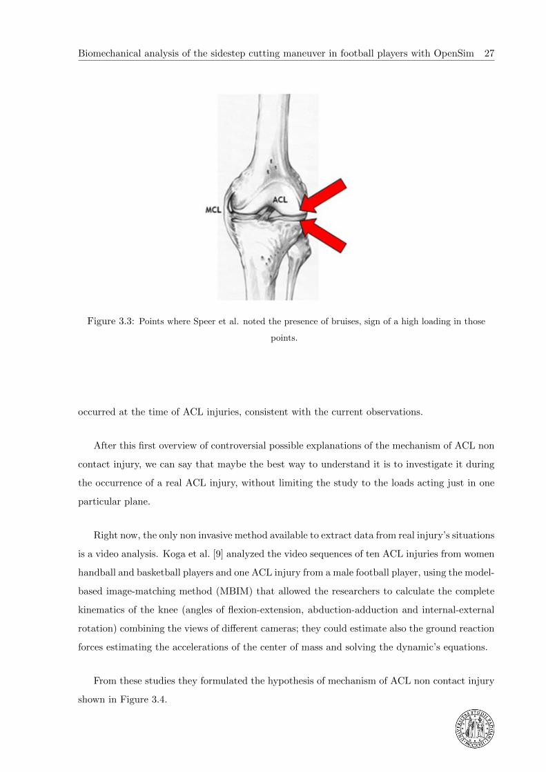
Biomechanical analysis of the sidestep cutting maneuver in football players with OpenSim 27
Figure 3.3: Points where Speer et al. noted the presence of bruises, sign of a high loading in those
points.
occurred at the time of ACL injuries, consistent with the current observations.
After this first overview of controversial possible explanations of the mechanism of ACL non
contact injury, we can say that maybe the best way to understand it is to investigate it during
the occurrence of a real ACL injury, without limiting the study to the loads acting just in one
particular plane.
Right now, the only non invasive method available to extract data from real injury’s situations
is a video analysis. Koga et al. [9] analyzed the video sequences of ten ACL injuries from women
handball and basketball players and one ACL injury from a male football player, using the model-
based image-matching method (MBIM) that allowed the researchers to calculate the complete
kinematics of the knee (angles of flexion-extension, abduction-adduction and internal-external
rotation) combining the views of different cameras; they could estimate also the ground reaction
forces estimating the accelerations of the center of mass and solving the dynamic’s equations.
From these studies they formulated the hypothesis of mechanism of ACL non contact injury
shown in Figure 3.4.
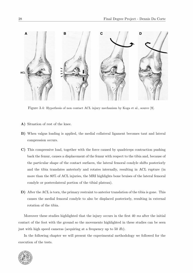
28 Final Degree Project - Dennis Da Corte
Figure 3.4: Hypothesis of non contact ACL injury mechanism by Koga et al., source [9].
A) Situation of rest of the knee.
B) When valgus loading is applied, the medial collateral ligament becomes taut and lateral
compression occurs.
C) This compressive load, together with the force caused by quadriceps contraction pushing
back the femur, causes a displacement of the femur with respect to the tibia and, because of
the particular shape of the contact surfaces, the lateral femoral condyle shifts posteriorly
and the tibia translates anteriorly and rotates internally, resulting in ACL rupture (in
more than the 80% of ACL injuries, the MRI highlights bone bruises of the lateral femoral
condyle or posterolateral portion of the tibial plateau).
D) After the ACL is torn, the primary restraint to anterior translation of the tibia is gone. This
causes the medial femoral condyle to also be displaced posteriorly, resulting in external
rotation of the tibia.
Moreover these studies highlighted that the injury occurs in the first 40 ms after the initial
contact of the foot with the ground so the movements highlighted in these studies can be seen
just with high speed cameras (acquiring at a frequency up to 50 Hz).
In the following chapter we will present the experimental methodology we followed for the
execution of the tests.
Biomechanical analysis of the sidestep cutting maneuver in football players with OpenSim 29
Chapter 4
Experimental methodology
4.1 Instrumentation
4.1.1 Motion capture system
In order to acquire the movement of the athletes performing the maneuver object of the study,
we needed to use a motion capture system; in our case the system used was a Peak Motus,
Version 9.2.0 (Peak Performance Technologies, Inc. USA) with 4 digital cameras Basler A602fc
(Basler AG Ahrensburg Germany) acquiring at 150 Hz with the characteristics shown in Table
4.1. An image of the cameras used can be seen in Figure 4.1.
There is the possibility to acquire at a higher frequency, reducing the resolution of the
sensor; the sampling frequencies permitted by Vicon Motus are 50, 60, 75, 80, 120, 125, 150,
200, 240, 250 and 300 Hz. In our case we used a sampling rate of 150 Hz with a resolution
horizontal/vertical of 536 x 400 pixels.
The athlete is wearing some passive reflecting markers in particular landmarks of the body
described in the marker protocol chosen for the test, the digital cameras acquire the execution
of the movement and the trajectories of the markers can be reconstructed during the processing
with the software Vicon Motus 9 (Vicon UK), an example of the process of recognition of the
markers is shown in Figure 4.2.

30 Final Degree Project - Dennis Da Corte
Figure 4.1: Basler A602fc camera.
Basler A602fc specifications:
Resolution horizontal/vertical (pixels) 656 x 490
Pixel Size horizontal/vertical 9.9 µm x 9.9 µm
Frame Rate 100 fps
Synchronization External trigger
Via the 1394 bus
Free-run
Exposure Control programmable via the 1394 bus
Housing Temperature 0 ◦C - 50 ◦C
Power Consumption (typical) 1.7 W
Weight (typical) 100 g
Sensor Technology Progressive Scan CMOS, global shutter
Sensor Size (optical) 1/2 inch
Sensor Type CMOS
Sensor Size [mm] 6.49 x 4.86
Table 4.1: Characteristics of Basler A602fc cameras.
Working with the contrast and the brightness, it is possible to distinguish the reflections
of the passive markers, because they are covered with a reflective material made of aluminum
powder. Starting from a manual detection of all the markers done by the user, the software
is able to follow the markers during the movement (if they can be seen in every frame) and
recognize their positions in the view of each camera.
Then, using a Direct Linear Transformation (DLT) the software is able to combine the views
of the different cameras in order to reconstruct the three-dimensional position of each marker

Biomechanical analysis of the sidestep cutting maneuver in football players with OpenSim 31
Figure 4.2: Example of the process of recognition of the markers in the Vicon Motus 9 environment.
frame by frame. We have to take care because the DLT method will not work if two cameras have
their optical axes at exactly 180◦. We know that, in order to be able to do all the reconstruction
of the trajectories of the markers, each marker has to be seen at least by two cameras in every
instant, according to the triangulation principle, and the higher is the number of cameras that
can see simultaneously a marker, the higher is the accuracy in the determination of its position.
Recording all the positions of the markers during the movement, the software can reconstruct
the trajectories of each marker and then, deriving once and twice with respect to time, also the
velocities and the accelerations. The results coming from the Motion Capture system are not
correct in absolute, but they are very dependent on the position of the cameras, the quality of
the calibration of the system, the errors and artifacts.
Position of the cameras:
As we said before if we want the Direct Linear Transformation (DLT) working, we have to
be sure that the angles between all the optical axes of the cameras has to be always different
from 180◦.
Then, as we said, in order to reconstruct correctly the trajectories of the markers, every
marker has to be seen in every frame by at least two cameras; this depends a lot on the position
and on the number of the cameras and, of course, on the nature of the movement. In general,
the higher is the number of cameras, the higher is the accuracy in the determination of the
markers position.
The position of the cameras depends a lot on the kind of movement and on the set of markers
that has been used and in general we have to take into account that during the execution of the

32 Final Degree Project - Dennis Da Corte
movement we should have a complete view of all the markers. In our case we used four cameras
fixed on easels at a height of more or less 1,70 m and disposed in a plane view as shown in Figure
4.3.
Figure 4.3: Plan view of the disposition of the four cameras and the force platform. It’s possible to see
also the longitudinal direction and the direction of the movement inclined at 60◦ with respect to the
longitudinal direction.
Calibration:
The calibration is the process that allows the system to fix a reference system and to generate
the relations that allow calculating the distances in a defined volume called volume of calibration.
First of all we put three reflecting markers on the floor defining the directions of the two
horizontal axes (perpendicular to each other) of the laboratory reference system (X and Y in
our case) as we can see in Figure 4.4.
Then we can assemble and place the control object called “32-point Frame” that is repre-
sented in Figure 4.5. This is composed by an easel with a central body where there are eight
rods attached: these sticks have four markers each placed at a known distance from each other.
It’s possible to extend the sticks adding more parts in order to increase the volume of control.
After making an acquisition of the control object and the three markers placed on the floor,
the user has to detect each marker and mark it with its name, in order to make the system
recognize it.
The horizontal axes of the laboratory reference system are detected using the three markers
placed on the floor and the vertical axis can be defined as the cross product of the two horizontal

Biomechanical analysis of the sidestep cutting maneuver in football players with OpenSim 33
Figure 4.4: Identification of the two horizontal axes X and Y of the laboratory reference system during
the process of calibration.
unitary vectors. The system knows how the control object is defined, because the coordinates of
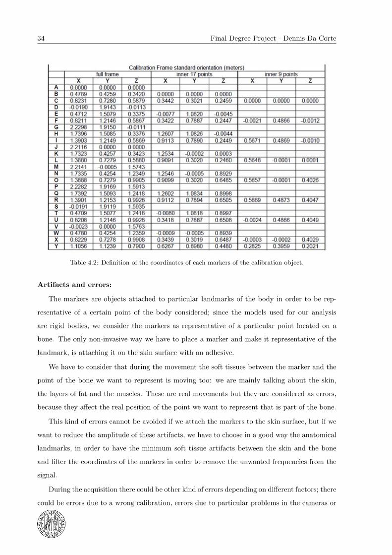
each marker are known as we can see in Table 4.2, so it is possible to calculate the coordinates
of all the points inside the volume of control.
Figure 4.5: The “32-point Frame” object used for the calibration.
34 Final Degree Project - Dennis Da Corte
Table 4.2: Definition of the coordinates of each markers of the calibration object.
Artifacts and errors:
The markers are objects attached to particular landmarks of the body in order to be rep-
resentative of a certain point of the body considered; since the models used for our analysis
are rigid bodies, we consider the markers as representative of a particular point located on a
bone. The only non-invasive way we have to place a marker and make it representative of the
landmark, is attaching it on the skin surface with an adhesive.
We have to consider that during the movement the soft tissues between the marker and the
point of the bone we want to represent is moving too: we are mainly talking about the skin,
the layers of fat and the muscles. These are real movements but they are considered as errors,
because they affect the real position of the point we want to represent that is part of the bone.
This kind of errors cannot be avoided if we attach the markers to the skin surface, but if we
want to reduce the amplitude of these artifacts, we have to choose in a good way the anatomical
landmarks, in order to have the minimum soft tissue artifacts between the skin and the bone
and filter the coordinates of the markers in order to remove the unwanted frequencies from the
signal.
During the acquisition there could be other kind of errors depending on different factors; there
could be errors due to a wrong calibration, errors due to particular problems in the cameras or
Biomechanical analysis of the sidestep cutting maneuver in football players with OpenSim 35
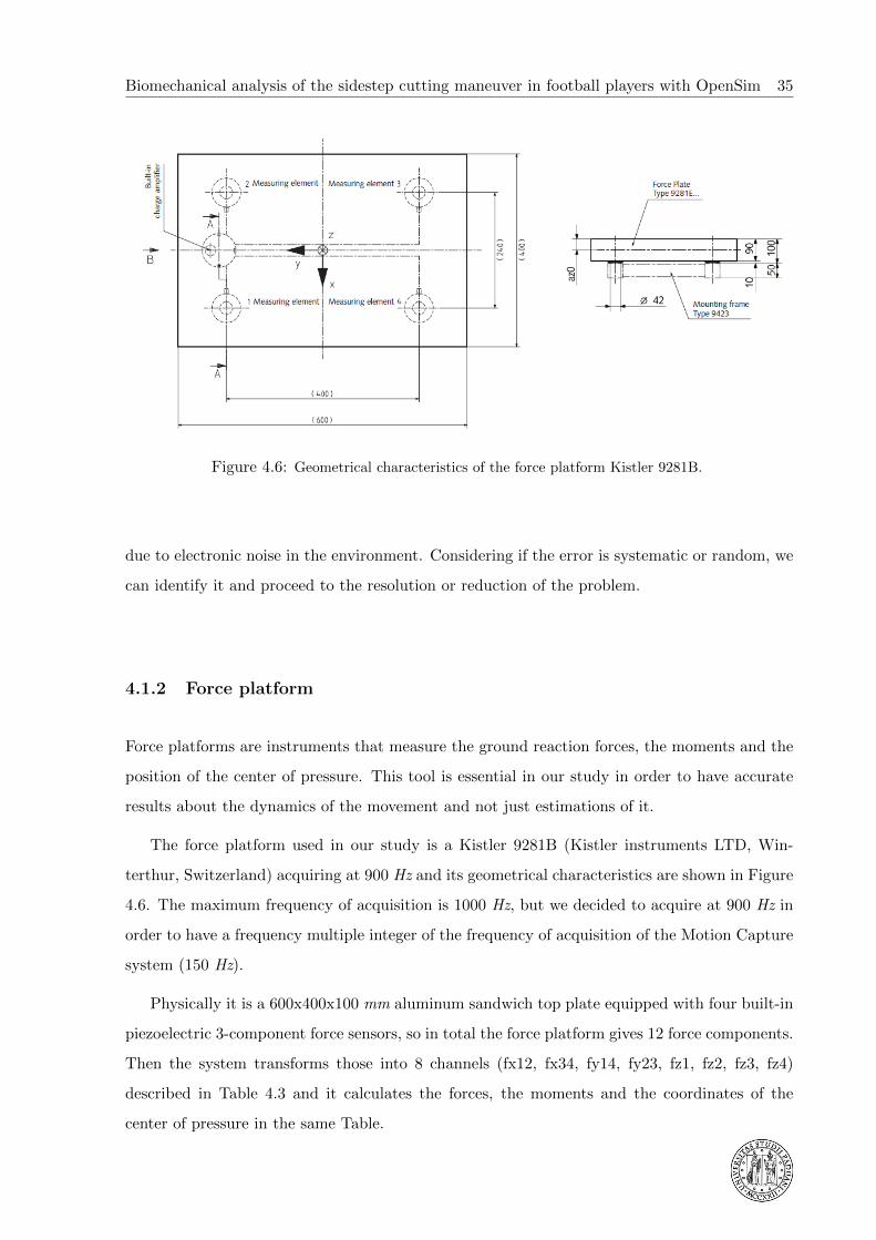
Figure 4.6: Geometrical characteristics of the force platform Kistler 9281B.
due to electronic noise in the environment. Considering if the error is systematic or random, we
can identify it and proceed to the resolution or reduction of the problem.
4.1.2 Force platform
Force platforms are instruments that measure the ground reaction forces, the moments and the
position of the center of pressure. This tool is essential in our study in order to have accurate
results about the dynamics of the movement and not just estimations of it.
The force platform used in our study is a Kistler 9281B (Kistler instruments LTD, Win-
terthur, Switzerland) acquiring at 900 Hz and its geometrical characteristics are shown in Figure
4.6. The maximum frequency of acquisition is 1000 Hz, but we decided to acquire at 900 Hz in
order to have a frequency multiple integer of the frequency of acquisition of the Motion Capture
system (150 Hz).
Physically it is a 600x400x100 mm aluminum sandwich top plate equipped with four built-in
piezoelectric 3-component force sensors, so in total the force platform gives 12 force components.
Then the system transforms those into 8 channels (fx12, fx34, fy14, fy23, fz1, fz2, fz3, fz4)
described in Table 4.3 and it calculates the forces, the moments and the coordinates of the
center of pressure in the same Table.

36 Final Degree Project - Dennis Da Corte
Table 4.3: Definition of the channels of the force platform and calculation of the main variables.
4.1.3 Electromyography
Electromyography (EMG) is a technique for evaluating and recording the electrical activity
produced by skeletal muscles [6]. An electromyograph detects the electrical potential (mV)
generated by muscles when they are activated.
There are two kinds of electromyography systems: the surface EMG that requires to attach
the electrodes on the skin, it is quite non-invasive but the accuracy of the results that can give

Biomechanical analysis of the sidestep cutting maneuver in football players with OpenSim 37
Figure 4.7: Mega WBA EMG system: above the receiver and below the sensors attached on the
charging/synchronizing module.
is low, and the needle EMG that requires the electrodes to be put under the skin and it is more
accurate but of course also more invasive.
In our study the electromyography data have not been used for any kind of evaluation, but
they have been collected too for any future kind of evaluation. For this purpose we used the 8
channels surface electromyography system Mega WBA (Mega Electronics LTD, Kupio, Finland)
shown in Figure 4.7. The system is composed by the sensors and the receiver.
Sensors:
Each sensor corresponds to one channel and is the set of one wireless transmitter and three
cables with connectors where disposable surface electrodes can be attached on; we can see a
representation of one sensor in Figure 4.8.
Each channel can work independently from the others and does not need any wire of con-
nection, neither for the supply, neither for the transmission of the data. This system does not
have a common ground for all the channels, but each channel has its own ground, this solution
requires one electrode more for each channel, but it allows a better modularity and compactness
of the system.
The wireless transmitter is needed to collect the signals from the electrodes and to send
them to the receiver; it contains the electronic circuit that is able to send the data wirelessly
and a battery, needed to make working the sensor without any supply wire; the battery can be

38 Final Degree Project - Dennis Da Corte
Figure 4.8: One of the sensor of the Mega WBA EMG system: the three electrodes and the wireless
transmitter.
recharged connecting the sensors to the charging module. The characteristics of the sensors are
shown in Table 4.4.
Mega WBA EMG sensors specifications:
Sampling rate 1000 Hz
CMRR Typ. 104 dB
Channels Up to 16
Sensor freq band 20-500 Hz (EMG model)
Data transfer Bluetooth 2.0 EDR
Power Internal rechargeable batteries
Weight 16 g / module
Size 35 x 35 x 15 mm
Electrodes Lead wires with snap connectors for disposable electrodes
Table 4.4: Characteristics of the sensors of the WBA Mega EMG system.
Receiver:
The receiver is an instrument that is able to collect all the wireless data coming from the
sensors and to transmit them through an analog cable to the computer. The characteristics of
the receiver are shown in Table 4.5.
It has to be considered that, since the data are passing from the sensors to the receiver
through a wireless connection, there is a delay of the data that arrive to the computer and the
real instant when they are collected. This delay has been quantified in 60 ms and it is corrected
manually by the user in the Vicon software.

Biomechanical analysis of the sidestep cutting maneuver in football players with OpenSim 39
Mega WBA EMG receiver specifications:
D/A conversion 16 bits
Analog output Yes, Isolated
Power supply 100-240 V, Medical Approved (UL60601) power supply
Interfaces Analog, Bluetooth
Table 4.5: Characteristics of the receiver of the WBA Mega EMG system.
4.1.4 Mechanical vibrations machine
To see which are the effects of mechanical vibrations on the execution of a sidestep cutting
movement, we needed a mechanical vibration machine and we used a ViBalance (Biomedic
System, Barcelona, Spain) that is shown in Figure 4.9.
This machine can produce three-dimensional mechanical vibrations in a frequency from 20
to 50 Hz and an amplitude from 1 to 2 mm. The characteristics of the ViBalance can be seen
in Table 4.6.
Figure 4.9: Mechanical vibrations machine ViBalance.

40 Final Degree Project - Dennis Da Corte
ViBalance specifications:
Motors (2) 0.18 KW, 3000 rpm
Frequency 20-50 Hz (adjustable Hz to Hz)
Pre-set Frequency 20,25,30,35,40,45,50 Hz
Amplitude HIGH (2 mm), LOW (1 mm) peak-to-peak
Maximal acceleration 7G
Weight 49 Kg
Dimensions 990 x 740 x 315 mm
Vibratory surface Diameter 698 mm
Maximum load 200 Kg
Maximum inclination 23◦ ± 2◦
Table 4.6: Characteristics of the mechanical vibrations machine ViBalance.
4.2 Execution of the test
The subjects that took part in these tests were footballers that had never had any injury at the
knee or at the ankle in the last months. Moreover any of them had never had any lesion in the
anterior cruciate ligament (ACL) before the tests. Before the execution of the test each subject
had to sign an informed consent and the ethics committee of the Catalan sport’s council licensed
the protocol of execution of the test.
4.2.1 Preparation of the tester
The preparation of the testers is essential in order to have good data concerning the kinematics
and the electromyography and has to be done in the most precise way possible.
First of all the anthropometric data of the subjects were collected, in particular the length
of the limbs and the mass. In this preliminary part of the subjects’ preparation, the places of
positioning of the electrodes were also signed.
Application of the EMG electrodes:
The application of the EMG electrodes it is an operation that in our case took more or less
20 minutes of time. The procedure of application of the electrodes is standard and it has been
collected and unified in the SENIAM project (Surface Electromyography for the Non-Invasive
Assessment of Muscles); the main guidelines used for the project have been taken from the
SENIAM website [18].

Biomechanical analysis of the sidestep cutting maneuver in football players with OpenSim 41
Before applying the electrodes, the skin has been prepared as shown in Figure 4.10: shaving
and cleaning with cotton and alcohol in order to reduce the impedance due to the hair, the
sebum and the sweat on the surface of the skin.
Figure 4.10: Preparation of the skin for the application of the electrodes: shaving and cleaning with
cotton and alcohol.
As we saw previously, for each muscle we want to collect the data, we need one EMG sensor
that has three electrodes each: two of them are collecting the potential passing along the skin
that will be treated passing through a differential or a double differential amplifier, the other one
is the ground electrode that gives the value of reference to the system. We can see a schematic
example of the treatment of the signals coming from the three electrodes in Figure 4.11.
Figure 4.11: Representation of the treatment of the data coming from the EMG electrodes with a
double differential amplifier.
Each electrode is attached to the shaved, cleaned and dried skin with its adhesive part then
the three electrodes and the transmitter are fixed to the limb with a porous gauze that allows
a better transmission of the data from the transmitter to the receiver.
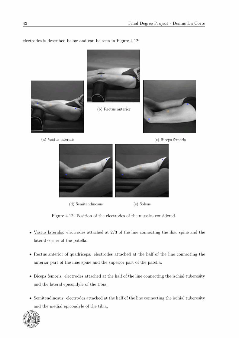
The muscles we are interested in studying are the vastus lateralis, rectus anterior of quadri-
ceps, biceps femoris, semitendinosus and soleus and the precise point of application of the
42 Final Degree Project - Dennis Da Corte
electrodes is described below and can be seen in Figure 4.12:
(a) Vastus lateralis
(b) Rectus anterior
(c) Biceps femoris
(d) Semitendinosus (e) Soleus
Figure 4.12: Position of the electrodes of the muscles considered.
• Vastus lateralis: electrodes attached at 2/3 of the line connecting the iliac spine and the
lateral corner of the patella.
• Rectus anterior of quadriceps: electrodes attached at the half of the line connecting the
anterior part of the iliac spine and the superior part of the patella.
• Biceps femoris: electrodes attached at the half of the line connecting the ischial tuberosity
and the lateral epicondyle of the tibia.
• Semitendinosus: electrodes attached at the half of the line connecting the ischial tuberosity
and the medial epicondyle of the tibia.
Biomechanical analysis of the sidestep cutting maneuver in football players with OpenSim 43
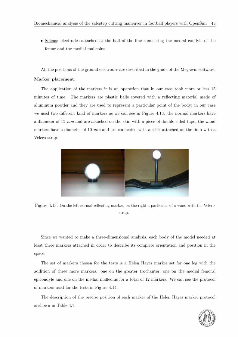
• Soleus: electrodes attached at the half of the line connecting the medial condyle of the
femur and the medial malleolus.
All the positions of the ground electrodes are described in the guide of the Megawin software.
Marker placement:
The application of the markers it is an operation that in our case took more or less 15
minutes of time. The markers are plastic balls covered with a reflecting material made of
aluminum powder and they are used to represent a particular point of the body; in our case
we used two different kind of markers as we can see in Figure 4.13: the normal markers have
a diameter of 15 mm and are attached on the skin with a piece of double-sided tape; the wand
markers have a diameter of 10 mm and are connected with a stick attached on the limb with a
Velcro strap.
Figure 4.13: On the left normal reflecting marker, on the right a particular of a wand with the Velcro
strap.
Since we wanted to make a three-dimensional analysis, each body of the model needed at
least three markers attached in order to describe its complete orientation and position in the
space.
The set of markers chosen for the tests is a Helen Hayes marker set for one leg with the
addition of three more markers: one on the greater trochanter, one on the medial femoral
epicondyle and one on the medial malleolus for a total of 12 markers. We can see the protocol
of markers used for the tests in Figure 4.14.
The description of the precise position of each marker of the Helen Hayes marker protocol
is shown in Table 4.7.

44 Final Degree Project - Dennis Da Corte
Figure 4.14: Set of markers used for the captures.
Helen Heyes marker protocol:
L. ASIS Placed directly over the left anterior superior iliac spine.
R. ASIS Placed directly over the right anterior superior iliac spine.
Sacrum Placed on the skin mid-way between the posterior superior iliac
spines (PSIS).
R. Femoral Wand A 4 inch wand placed on the right leg over the lower lateral 1/3
surface of the thigh, just below the swing of the hand.
R. Femoral epicondyle Placed on the lateral epicondyle of the right knee.
R. Tibial Wand A 4 inch wand placed over the lower 1/3 of the shank to determine
the alignment of the ankle flexion axis.
R. Malleolus Placed on the lateral malleolus along an imaginary line that passes
through the transmalleolar axis.
R. Metatarsal Head II Placed over the second metatarsal head, on the mid-foot side of
the equinus break between fore-foot and mid-foot.
R. Heel Placed on the calcaneus at the same height above the plantar
surface of the foot as the toe marker.
Table 4.7: Description of the positions of the markers of the Helen Heyes protocol.

Biomechanical analysis of the sidestep cutting maneuver in football players with OpenSim 45
4.2.2 Protocol of execution of the tests
The tests were executed mainly in order to see what are the differences between the move-
ments performed pre and post vibrations; after the application of the EMG system and the
reflecting markers, the subject performed three sidestep cutting movements, with one minute
of recovery between each other. After the execution of the three sidestep cutting movements
pre-vibrations and five minutes of recovery, the subject made the warming-up with full body
mechanical vibrations (VCC) and then performed three more sidestep cutting movements.
A block diagram representing tasks made during the execution of the tests can be seen in
Figure 4.15.
All the subjects performed the tests using indoor football shoes during the warming-up and
during the sidestep cutting movements.
Figure 4.15: Block diagram representing the tasks made during the execution of the tests.
Protocol of the sidestep cutting maneuver:
The execution of the sidestep cutting maneuver in our case took more or less 5 minutes for
each session. This kind of movement is particularly problematic for the ACL noncontact injuries,
especially according with the mechanism of injury we presented in the previous chapters.
The subject jumped from a step of 30 cm and the frontal border of this step was located at a
distance equal to 2/3 of the height of the subject from the center of the force platform, landing
on the force platform with the dominant leg. This first jump was executed in a longitudinal
direction, then the subject made the second part of the jump along a direction inclined at 60◦
with respect to the longitudinal direction in the side of the non-dominant leg, pushing with the
dominant leg. Some frames of the execution of the maneuver and a planar scheme of it can be
seen in Figures 4.16 and 4.17.

46 Final Degree Project - Dennis Da Corte
(a) Intitial phase of the
movement
(b) Landing with the dominant
leg
(c) Maximum flexion of the
knee
(d) End of the contact of the
dominant leg
(e) Landing with the
non-dominant leg
Figure 4.16: The most significant frames of the execution of the sidestep cutting maneuver.
Figure 4.17: Planar scheme (top view) of the execution of a sidestep cutting maneuver.

Biomechanical analysis of the sidestep cutting maneuver in football players with OpenSim 47
Protocol of warming-up with mechanical vibrations:
The warming-up with mechanical vibration is an operation that in our case took more or less
15 minutes of time. The warming-up with mechanical vibrations was performed on a vibratory
platform with a frequency of vibration of 30 Hz and an amplitude of 2 mm. These values had
been chosen according with a study of Cardinale and Lim 2003 [14] where they explained that
with a frequency of 30 Hz the EMG activation of the vastus lateralis of the quadriceps is the
highest. The same values of frequency and amplitude had been used also in other studies with
the application of full body mechanical vibrations.
The warming-up consisted in six series of squats on one leg of 45 seconds each with 60 seconds
of recovery between each other; these six series of squats were divided in three series of dynamic
squats and three series of static squats as shown in Figure 4.18.
In the three series of dynamic squats the subject performed squats lasting 5 seconds each
(three seconds in eccentric action and two seconds in concentric action), with a maximum knee
flexion angle of 90◦. The time of flexion and extension was controlled using a metronome. In
the three series of static squats, the subject maintained the static position of flexion of the knee
at 90◦ (isometric squat).
During the execution of the warming-up the subjects had a rod that helped them to maintain
the balance staying on the vibratory platform. In Figure 4.19, we can see how the squats have
been performed by two of the analyzed subjects.
Figure 4.18: Protocol of execution of the six series of squats during the warming-up with mechanical
vibrations.

48 Final Degree Project - Dennis Da Corte
Figure 4.19: Execution of the squats with mechanical vibrations: on the left dynamic squat, on the
right static squat.
In the following chapter we will present the numerical part of the work explaining in details
the choices made, the problems we find and all the procedure followed during the running of the
numerical simulations with OpenSim.

Biomechanical analysis of the sidestep cutting maneuver in football players with OpenSim 49
Chapter 5
Numerical methodology
5.1 Presentation of OpenSim
5.1.1 Capabilities of OpenSim
OpenSim [21] is a freely available software package created and certificated by the National
Center for Simulation in Rehabilitation Research of the Stanford University that enables users
to build, exchange, and analyze computer models of the musculoskeletal system and dynamic
simulations of movement.
The core software is written in C++, and the Graphical User Interface (GUI) is written in
Java. OpenSim’s plugin technology makes possible to develop customized controllers, analyses,
contact models, and muscle models among other things. The user can analyze existing models
and simulations or develop its own new models and simulations.
According to this idea of the first developers of the Stanford University, there is a community
[20] in which it’s possible to share for free experiences, models, tutorials, guides, plugins, advices
and many other things between the members of the community.
Some of the most useful features of the software include:
• Scaling the size of a musculoskeletal model;
• Performing inverse kinematics analysis to calculate joint angles from marker positions;
• Performing inverse dynamics analysis to calculate joint moments from joint angles and
external forces;
• Generating forward dynamics simulations of movement;
• Analyzing dynamic simulations;

50 Final Degree Project - Dennis Da Corte
• Calculating muscle forces and activations;
• Plotting results of your analysis;
• Taking pictures of musculoskeletal models and making animated movies.
5.1.2 How OpenSim works
To make an analysis with OpenSim first of all we need a model of the musculoskeletal system
of the body we want to analyze. There are a lot of models already created in the folder of
OpenSim and in the website [20] there are many other models developed by the users ready to
be downloaded for free.
The models are made of rigid bodies in the three-dimensional space; each of them has its own
reference system and its geometrical and physical properties are described through differential
equations. These rigid bodies can’t move in the space as they want, but there are some constraint
conditions, described through boundary conditions, that definewhich are the movements allowed
to each child body with respect to the parent body (conditions on the reference systems). In the
model there are also muscles with all their geometrical and physical characteristics described
through other differential equations based on the Hill’s model.
The data coming from the motion capture system give the instantaneous position of some
points attached to each body segment so, since each body is a rigid body in the three-dimensional
space, we need at least three conditions for each body to describe completely its position and
orientation in the space in every instant. The data coming from the force platform give more
boundary conditions to the differential motion equations that have to be solved during the
analysis.
5.2 Procedure of the numerical simulation
5.2.1 Preparation of the data
The data coming from the force platform, the motion capture system and the EMG system
has been acquired with Vicon Motus software and, after reconstructing the trajectories of each
marker, they have been saved in a *.c3d file.
This format of file cannot be read immediately from OpenSim as an input; so it’s needed to
process the files through Matlab. There are some scripts already created by users that can be

Biomechanical analysis of the sidestep cutting maneuver in football players with OpenSim 51
downloaded for free from the OpenSim community [20] and allow the user to create all the data
files needed to run the simulations with OpenSim.
In our case, the script for the processing of the force platform data was not compatible with
the force platform used. This is because the scripts are made just for a 6 channels force platform,
but the force platform used for the project has 8 channels. To solve this problem without
spending too much time with Matlab, we decided to save from the Vicon Motus software an
*.xls file containing all the data from the force platform already processed, and then converting
this file separately in the format needed by OpenSim. The scheme of the data conversion made
can be seen in Figure 5.1.
Figure 5.1: Scheme of the conversion of the data to the formats used by OpenSim.
Sometimes it can happen that in the marker trajectories there is a singular point (due to a
flickering of the marker) and this could bring to big errors during the execution of the simulations.
So, it’s better to plot the trajectory of each marker before starting any simulation in order to
see if there is any singular point and, in that case, correct manually the value to have a good
shape of the curve. To do this, we just replaced the wrong value with the mean of the previous
and the following values.
In Figure 5.2 it’s possible to see an example of the trajectory of a marker with the problem
of singularity and the same curve after replacing the wrong value.
It’s not suggested to filter the trajectories of the markers before starting the analysis because
this could introduce some problems also in the Inverse Kinematics analysis. Instead of filtering
the coordinates of the markers it’s possible to filter the results of the Inverse Kinematics analysis
in order to remove the high frequency noise.
The data coming from the force platform have been filtered with a Butterworth low pass
filter of the third order with a cutting frequency of 15 Hz. The frequency of cutting is the
same used in another researches about sidestep cutting [4] and it should reduce the noise and

52 Final Degree Project - Dennis Da Corte
(a) Example of problem of singularity in the
trajectory of a marker.
(b) Trajectory of the marker after the manual
correction of the signularity.
Figure 5.2: Example of the trajectory of a marker before and after the correction of a
singuarity.
the artifacts of impact typical of this kind of movement. It’s possible to see an example of the
vertical component of the ground reaction force before and after filtering in Figure 5.3. Note the
reduction of the peak of the impact, the reduction of the noise and the appearance of negative
values.
(a) Example of raw vertical force. (b) Example of vertical force filtered.
Figure 5.3: Example of vertical component of the ground reaction force before and after
filtering.
One important parameter that we wanted to preserve during the analysis was the instant of
first contact of the foot with the force platform; this is conventionally considered as the instant
when the vertical force is greater than 10 N. For this purpose, we tried to use different orders of
filter paying attention to the instant of first contact of the foot with the force platform and we

Biomechanical analysis of the sidestep cutting maneuver in football players with OpenSim 53
saw that with the third order filter this parameter was closer to the original one; we can observe
it in Figure 5.4.
-100
-50
0
50
100
150
200
250
300
0,1 0,11 0,12 0,13 0,14 0,15 0,16 0,17 0,18 0,19 0,2
forc
e [
N]
!me [s]
Par!cular_Fz
Raw
Order 1
Order 2
Order 3
10 N constant
-100
-50
0
50
100
150
200
250
300
0,1 0,11 0,12 0,13 0,14 0,15 0,16 0,17 0,18 0,19 0,2
forc
e [
N]
!me [s]
Par!cular_Fz
Raw
Order 1
Order 2
Order 3
10 N constant
Figure 5.4: Comparison in the zone of first contact, between the raw vertical force and the same data
filtered with Butterworth low pass filters with a cut off frequency of 15 Hz but with different orders. It
can be observed that the instant of first contact with the floor (Fz ≥ 10 N) in the case of using the
third order filter is closer to the one corresponding to the raw data.
This solution brought to a diagram of the vertical force with a negative part before the
instant of first contact. Although know that this is not possible in the reality, we accept it
because we are not using the forces before the first contact of the foot in our analysis.
5.2.2 Model
The biomechanical model used in the analysis is the “Gait2392 Simbody” (downloadable from
[20]) without the torso and the left leg and with 3 degrees of freedom at the knee joint. The
model can be seen in Figure 5.5.
The model is described in a code where we can see how the bodies are defined, which are the
reference systems, which are the characteristics of the joints, how the muscles are defined and
so on. Some small changes to the model can be made using the GUI (Graphical User Interface)
but, if more significant changes are needed, then the code that describes the model has to be
edited manually using a text editor.
The first change we made to the original code was to delete the bodies not needed (torso
and left leg) with all the muscles attached to them. As default settings of the model the knee

54 Final Degree Project - Dennis Da Corte
Figure 5.5: Biomechanical model used for the analysis coming from the “Gait2392 Simbody” with
some changes.
joint had just 1 DOF (flexion), but in our case it was interesting to have some information
also about the adduction and the internal rotation, considering which is the mechanism of ACL
injury described in the chapter 2. So, in the code we just added the other two degrees of freedom
of abduction and internal rotation in order to have the three degrees of freedom at the knee.
A range of motion of 0,8 radians (+0, 4/−0, 4 radians each) was given to the motions in order
to capture also non-physiologically consistent movements (we can consider as physiologically
consistent a maximum abduction angle around 10◦ and a maximum rotation angle around 15◦).
Some preliminary simulations were made in parallel with three different models in order to see
which of them was realistic enough:
• Model with flexion of the knee (1 DOF);
• Model with flexion and adduction of the knee (2 DOF);
• Model with flexion, adduction and internal rotation of the knee (3 DOF);
The results concerning the internal rotation were not physiologically consistent, but the
adduction’s ones were good, so at the end it was decided to use the model with two DOF at the
knee joint: flexion and adduction.

Biomechanical analysis of the sidestep cutting maneuver in football players with OpenSim 55
Even if the angles of the adduction obtained in the preliminary simulations were physiolog-
ically consistent, we have to consider that the error that can be made from the motion capture
system in determining the angles (around 5◦ in an acceptable case [12]) is quite big if compared
to the range of the adduction movement, so we can think to trust more in the tendency of the
adduction instead of in the absolute value of it.
In the preliminary simulations also a muscle analysis was made and it was possible to notice
a discontinuity in the lever arm of the lateral and medial gastrocnemius. Since the Static
Optimization is quite sensible to discontinuities in the lever arm of the muscles, we decided to
create a wrapping surface to be placed under the two gastrocnemius muscles.
A wrapping surface is a surface where some muscles indicated by the user can lean during
the movement. These two muscles in the original model were defined in the following way:
• As straight lines between two points in the range of flexion of the knee from 120◦ to 45◦;
• As straight lines passing through three points in the range of flexion of the knee from 45◦
to −10◦.
So when the knee passed through the angle of 45 degrees of flexion the definition of these
two muscles changed instantly from a straight line to a broken line, that is why there was the
discontinuity on the lever arms.
The wrapping surface created is a portion of cylinder where the muscles can lean when the
knee is in the range of flexion from −10◦ to 45◦; the definition of this surface has been introduced
in the code where the two muscles are defined. We can see the two muscles before and after
adding the wrapping surface in Figure 5.6.
We have moreover to consider that with the set of markers we used, we don’t have any
information about the movement of the fingers, so the “2nd metatarsal head” marker has been
attached to the calcaneus body and the “mtp angle” has been locked during the simulations.
In the preliminary simulations we also noticed that the Static Optimization couldn’t converge
to a solution; the problem was due to the fact that in some joints all the muscles acting with
their maximum isometric force and their lever arms were not enough to make the total joint
moment.
This problem is quite complex and will be presented later in the section dedicated to the
Static Optimization. Right now we can say that in order to solve this problem the maximum
isometric force of all the muscles was multiplied by 2,5.

56 Final Degree Project - Dennis Da Corte
Figure 5.6: The lateral and medial gastrocnemius as defined in the original model on the left and as
defined with the wrapping surface on the right.
So, the following list presents the changes made to the original model at the end of the
preliminary simulations:
• The torso and the left leg with all the muscles attached to them have been removed;
• Three degrees of freedom have been considered at the knee (flexion, adduction and internal
rotation);
• A wrapping surface to solve the discontinuity of lever arm on the lateral and medial
gastrocnemius muscles has been adeed;
• The maximum isometric force of all the muscles has been multiplied by a factor 2,5;
• The “knee rotation” angle and the “mtp angle” have been locked to the value of zero.
5.2.3 Scaling tool
The scaling is a very important multi step operation in the execution of the simulations. This
tool allows the user to:
• Change the dimensions of each body of the virtual model according to the dimension of
each body of the real subject;
• Adjust the positions of the most unsure model markers according to the experimental ones
from the static acquisition.
Biomechanical analysis of the sidestep cutting maneuver in football players with OpenSim 57
To start with the scaling operation, first of all we needed to define a set of markers attached to
the model; the positions of these model markers had to be as close as possible to the anatomical
landmarks where the experimental markers were attached. Moreover these markers needed to
have the same names as the markers in the *.trc file and it had to be specified to which body
they belong.
During the scaling operation we needed to set the mass of our model. The anthropometric
measurements made before starting the execution of the tests could give us the mass of the full
body of each subject, but our model was just composed by the pelvis and one leg.
In order to have an estimation of the model’s mass , we used the relations of Zatsiorsky-De
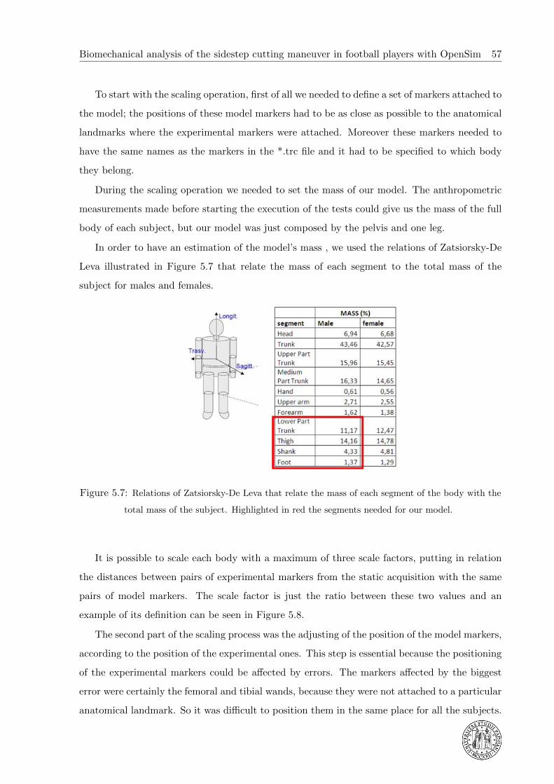
Leva illustrated in Figure 5.7 that relate the mass of each segment to the total mass of the
subject for males and females.
Figure 5.7: Relations of Zatsiorsky-De Leva that relate the mass of each segment of the body with the
total mass of the subject. Highlighted in red the segments needed for our model.
It is possible to scale each body with a maximum of three scale factors, putting in relation
the distances between pairs of experimental markers from the static acquisition with the same
pairs of model markers. The scale factor is just the ratio between these two values and an
example of its definition can be seen in Figure 5.8.
The second part of the scaling process was the adjusting of the position of the model markers,
according to the position of the experimental ones. This step is essential because the positioning
of the experimental markers could be affected by errors. The markers affected by the biggest
error were certainly the femoral and tibial wands, because they were not attached to a particular
anatomical landmark. So it was difficult to position them in the same place for all the subjects.

58 Final Degree Project - Dennis Da Corte
Figure 5.8: Example of the process of scaling of the length of the femurs: the distance between pairs of
markers in the model divided by the distance between the same pairs of experimental markers is equal
to the scale factor.
The position of all the other markers was referred to a particular landmark of the body, therefore
the positioning could be more accurate than the wand’s ones.
During this operation it is important to give a weight to each marker: the higher is the
weight of a marker, the better the experimental marker should be matching the position of the
model marker. Taking into account of this idea, the tibial wand and the femoral wand markers
had a very low weight. It is also possible to give some additional conditions on the coordinates
of the joints, if we know the precise value that they should have during the static pose.
The scaling is an iterative operation so, after the process of changing the dimension of the
bodies and adjusting of the positions of the markers, we had to go on reiterating these two
operations until the position’s RMS error that describes the quality of the markers’ adjustment
became close to a couple of millimeters.
5.2.4 Inverse Kinematics
With this tool it is possible to make the model reproducing frame by frame the movement of the
markers captured from the motion capture system, as illustrated in Figure 5.9, and to calculate
the joint angles.

Biomechanical analysis of the sidestep cutting maneuver in football players with OpenSim 59
(a) Intitial phase of the
movement
(b) Landing with the dominant
leg
(c) Maximum flexion of the
knee
(d) End of the contact of the
dominant leg
Figure 5.9: Model reproducing the movement of the experimental markers: the most
significant frames of the execution of the sidestep cutting maneuver of one subject.
It is possible to find frame by frame the model’s pose that best matches the position of the
experimental markers. The concept of best matching can be expressed as an objective function
that has to be minimized as we can see here:
minq
∑i∈markers
wi‖xiexp − xi(q)‖2 +∑
j∈unprescribed coords
ωj(qexpj − qj)2
(5.1)
qj = qexpj for all prescribed coordinates j
where:[‖xiexp − xi(q)‖2
]is the square error on the position of each marker;[
(qexpj − qj)2]
is the square error on the determination of each coordinate.
These two components of the objective function have to be weighted setting a weight (wi

60 Final Degree Project - Dennis Da Corte
and ωj), according with how sure we are about the position of each marker or about the value
of each coordinate.
In Table 5.1 rimmed in red, we can see how we can classify the quality of the results of an
Inverse Kinematics analysis.
Table 5.1: Classification of the quality of the analysis. Adapted from [12].
Since we did not filter the coordinates of the markers given as input to the Inverse Kinematics
analysis, before analyzing the results coming from this analysis it’s better to save a copy of them
and filter them with a Butterworth low pass filter of the third order with a cutting frequency of
15 Hz as suggested in [4].
5.2.5 Inverse Dynamics
The Inverse Dynamics tool allows the user to determine the net forces and torques at each joint
responsible for a given movement (the moments that can balance the external loads); a simplified
example of this analysis can be seen in Figure 5.10.
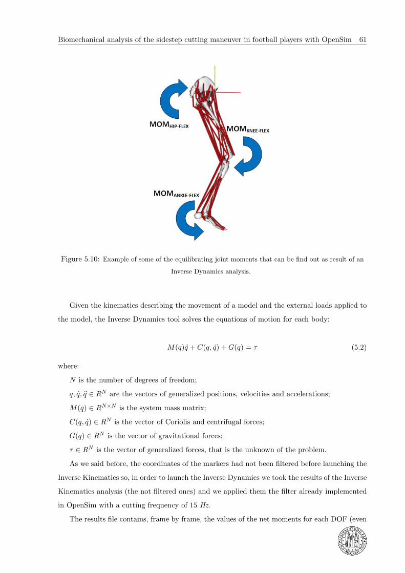
Biomechanical analysis of the sidestep cutting maneuver in football players with OpenSim 61
Figure 5.10: Example of some of the equilibrating joint moments that can be find out as result of an
Inverse Dynamics analysis.
Given the kinematics describing the movement of a model and the external loads applied to
the model, the Inverse Dynamics tool solves the equations of motion for each body:
M(q)q + C(q, q) +G(q) = τ (5.2)
where:
N is the number of degrees of freedom;
q, q, q ∈ RN are the vectors of generalized positions, velocities and accelerations;
M(q) ∈ RN×N is the system mass matrix;
C(q, q) ∈ RN is the vector of Coriolis and centrifugal forces;
G(q) ∈ RN is the vector of gravitational forces;
τ ∈ RN is the vector of generalized forces, that is the unknown of the problem.
As we said before, the coordinates of the markers had not been filtered before launching the
Inverse Kinematics so, in order to launch the Inverse Dynamics we took the results of the Inverse
Kinematics analysis (the not filtered ones) and we applied them the filter already implemented
in OpenSim with a cutting frequency of 15 Hz.
The results file contains, frame by frame, the values of the net moments for each DOF (even

62 Final Degree Project - Dennis Da Corte
Figure 5.11: Example of force-sharing problem in a simplified model of the ankle. If we don’t add any
additional condition, this problem has an infinite number of solutions.
if it’s locked) and the values of the three moments and the three forces at the pelvis. In our
case, the forces and moments at the pelvis are related to the contact between the pelvis and the
upper part of the body and between the pelvis and the left leg, which are were included in our
system.
5.2.6 Static Optimization
The Static Optimization tool is an extension to Inverse Dynamics that further resolves the net
joint moments into individual muscle forces frame by frame. The particularity of this process
is that the movement is divided in frames and the problem of muscular distribution is solved in
each frame as it would be static.
With the results of the Inverse Dynamics we know the net moment at a precise joint; we
know that this net moment has to be given by the sum of the forces of the muscles acting on
the joint multiplied by the lever arm of the muscles with respect to the joint.
This kind of problem, known as force-sharing problem has an infinite number of solutions
because, for each DOF, there is an equation of equilibrium with nm variables, where nm is the
number of muscles acting on that joint according with that DOF considered. An example of
this problem of forces repartition can be seen in Figure 5.11.
In order to find a unique solution we need another condition that in our case is an objective
function to be minimized. This objective function is represented by the sum of the activation of

Biomechanical analysis of the sidestep cutting maneuver in football players with OpenSim 63
the muscles acting on the precise joint we are considering, according to the precise DOF we are
looking for, at the power p that can be defined by the user. This is the objective function used
by OpenSim:
J =nm∑m=1
(am)p (5.3)
where am is the activation of the mth muscle. The suggestion of minimizing a function dependent
on the muscular activation comes from the idea that maybe the human body tries to make the
muscles working as less as possible to do a particular movement in order to save energy. We
don’t know if this is what really happens in the human body, and we can’t say that all the
subjects are responding to this mechanism of activation. This is just one possible way to solve
the muscle force-sharing problem, which is accepted by the scientific community. In our case we
used a coefficient p=2 that is the most common value find in literature.
OpenSim gives the possibility to choose between two different muscle models, depending on
how much we want the analysis to be accurate.
• Simple model without pennation (ideal actuator) that can be seen in Figure 5.12;
• Model of the contraction dynamics that can be seen in Figure 5.13.
This ideal actuator model is based on these main hypotheses:
• The tendon is infinitely stiff;
• The force produced by the muscle is not dependent on its velocity or length;
• The muscle fibers are acting on the same direction of the tendon.
Figure 5.12: Ideal actuator muscle model.
The force of the tendon can be expressed in the following way:
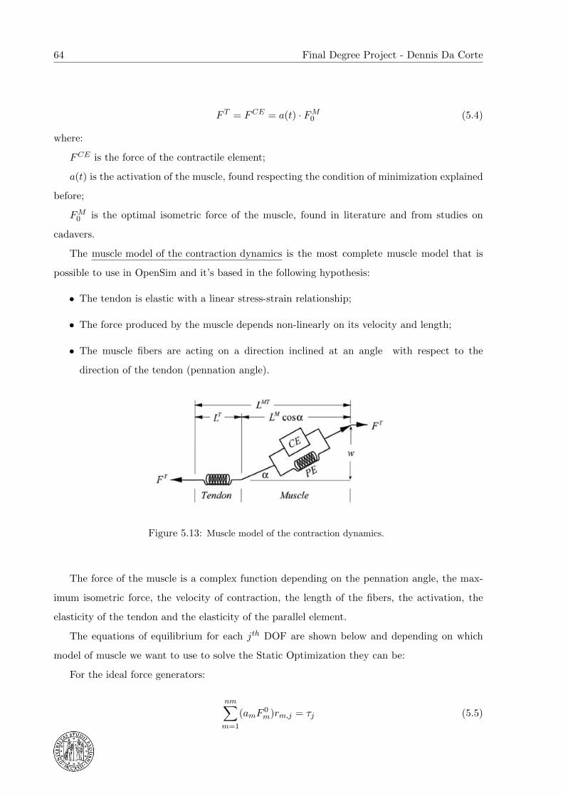
64 Final Degree Project - Dennis Da Corte
F T = FCE = a(t) · FM0 (5.4)
where:
FCE is the force of the contractile element;
a(t) is the activation of the muscle, found respecting the condition of minimization explained
before;
FM0 is the optimal isometric force of the muscle, found in literature and from studies on
cadavers.
The muscle model of the contraction dynamics is the most complete muscle model that is
possible to use in OpenSim and it’s based in the following hypothesis:
• The tendon is elastic with a linear stress-strain relationship;
• The force produced by the muscle depends non-linearly on its velocity and length;
• The muscle fibers are acting on a direction inclined at an angle with respect to the
direction of the tendon (pennation angle).
Figure 5.13: Muscle model of the contraction dynamics.
The force of the muscle is a complex function depending on the pennation angle, the max-
imum isometric force, the velocity of contraction, the length of the fibers, the activation, the
elasticity of the tendon and the elasticity of the parallel element.
The equations of equilibrium for each jth DOF are shown below and depending on which
model of muscle we want to use to solve the Static Optimization they can be:
For the ideal force generators:
nm∑m=1
(amF0m)rm,j = τj (5.5)

Biomechanical analysis of the sidestep cutting maneuver in football players with OpenSim 65
For the muscle model of the contraction dynamics:
nm∑m=1
[amf(F 0
m, lm, vm)]rm,j = τj (5.6)
where:
nm is the number of muscles of the model;
am is the activation level of the mth muscle at a discrete time step;
F 0m is the maximum isometric force of the mth muscle;
lm is the instantaneous length of the muscle;
vm is the shortening velocity of the muscle;
f(F 0m, lm, vm) is the relation between force-length-velocity for the muscle;
rm,j is the moment arm of the muscle about the jth joint axis;
τj is the torque acting about the j th joint axis.
In our case in the preliminary simulations the Static Optimization using the ideal actuators
muscle model and the parameters of the original model “Gait2392 Simbody” could not converge.
This happened because the muscles could not produce enough force to balance the joint moments.
This can be seen well in Figure 5.14, an example of comparison between the knee flexion
moment coming from the Inverse Dynamics analysis and the maximum knee flexion moment
that can be given by the muscles acting with their maximum isometric force and using the ideal
actuator model. It’s possible to see that in a portion of time the moment at the joint is greater
than the maximum moment that can be given by the muscles.

66 Final Degree Project - Dennis Da Corte
Figure 5.14: Example of a comparison between the moment of flexion at the knee coming from the
Inverse Dynamics analysis and the maximum moment of flexion that can be given by the muscles.
We have to take care that the reasoning made here is true just if we consider the ideal
muscle model, where the maximum force that can be produced by a muscle is exactly equal to
the maximum isometric force (it’s like treating each frame of the movement as an instant where
we have just isometric action).
If we take into account the dependence of the force on the velocity, the maximum force that
a muscle can product is not always the maximum isometric one, but depends on the velocity of
shortening/lengthening as it can seen in Figure 5.15. In fact for values of abscissa greater than
zero we have eccentric action (lengthening) and the maximum force is greater than the maximum
isometric one, for values of abscissa lower than zero we have concentric action (shortening) and
the maximum force is lower than the maximum isometric one.
The inconsistency we saw before in Figure 5.14 between the moment at the joint and the
maximum moment that can be given by the muscles could be explained in the following way:
• The data used to create the models are taken from cadavers, so we can think that the
strength of a dead tissue is lower than a live one;
• The original model “Gait2392 Simbody”, as the name says, it’s made to analyze the gait,
a movement that for sure causes lower stress on the muscles than the sidestep cutting,
characterized by a high dynamic and an explosive force action;

Biomechanical analysis of the sidestep cutting maneuver in football players with OpenSim 67
Figure 5.15: Ideal dependence of the force of the muscle on the velocity of extension.
• The model is made to describe the body of a normal person but the subjects used for the
tests had a muscle tone greater than a normal person, so probably they can not be well
represented by the model.
Considering all these aspects, it was decided to increase the maximum isometric force of
all the muscles in the same way. After some simulations, we decided to multiply the maxi-
mum isometric forces of all the muscles by 2,5 because this constant could ensure to solve the
inconsistency shown in Figure 5.14.
After modifying manually the maximum isometric force of the muscles, the Static Optimiza-
tion could converge. In this case the process succeeded just using the ideal actuator muscle
model, so without considering the dependence between force, length of the fibers and velocity
of contraction.
Just increasing the maximum isometric force of the muscles without optimizing the fiber
length and other muscular parameters, could bring the muscles to work far from their condition
of optimal force (around the peak of the curve shown in Figure 5.16).
For our study the solution obtained with the ideal actuator muscle model can be considered
good enough, anyway we also tried to use the muscle model of contraction dynamics optimizing

68 Final Degree Project - Dennis Da Corte
Figure 5.16: Dependence of the force of the muscle (normalized on the maximum isometric force) on
the instantaneous length (normalized on the optimal length).
the muscular parameters under the following simplified hypotheses:
• We wanted the muscles to be working around their condition of optimum with respect to
the fiber length, this means to be around the peak of the curve shown in Figure 5.16, so
where LM/LM0 ∼ 1;
• In order to optimize the optimal length of each muscle we considered a model with rigid
tendon and a pennation angle constant during the movement, corresponding to the pen-
nation angle at the optimal length of the muscle α0.
The length of the muscle and tendon (LMT ) has been taken from a Muscle Analysis for one
test of one subject, frame by frame for each muscle, the length of the tendon (LT ) has been taken
from the scaled model and is a constant (because the tendon is rigid in this model) and also
the pennation angle has been taken from the scaled model (it is constant because we decided to
take the pennation angle at the optimal length of the muscle).
The length of the muscle (LM ) could be calculated frame by frame in the following way:

Biomechanical analysis of the sidestep cutting maneuver in football players with OpenSim 69
LM =LMT − LT
cosα0(5.7)
Then, for every muscle, a mean of all the values of LM calculated at each time step was made,
and we considered this equal to the optimal fiber length, according with the first hypothesis
made:
LM0 ∼ LM
med (5.8)
In the model with the maximum isometric forces multiplied by 2,5 the optimal fiber length
of all the muscles was changed manually with the LM0 obtained in this way and the Static
Optimization was run using the muscle model of the contraction dynamics.
We have to take care that this approach is an optimization and in the reality the muscles
are never working all together in their optimal conditions. We have moreover to consider that
this optimization depends on the subject and on the particular kinematic of the test.
From a comparison of the results obtained with the two muscle models, we could see that
the two approaches did not give the same results, anyway it is not possible to say that one of
the two approaches is better than the other one: they are equally incorrect because they are
using simplified hypotheses in order to calculate the muscle forces. The two approaches can be
both considered good enough for our pilot study and they would need a comparison with the
results of the EMG system in order to verify their reliability. For our simulations we decided to
use the ideal actuator muscle model because this is the most time saving approach.
In the following chapter we will present the experimental results obtained and we will discuss
them, trying to connect them with the aspects related to the occurrence of ACL non contact
injuries.

70 Final Degree Project - Dennis Da Corte

Biomechanical analysis of the sidestep cutting maneuver in football players with OpenSim 71
Chapter 6
Experimental results and discussion
Before starting the quantitative analysis of the results obtained, a qualitative analysis has been
done in order to see if there was any significant difference between the subjects. From this
preliminary analysis it was possible to see that the techniques of execution of the sidestep
cutting maneuver were quite different among the subjects. Looking at the execution of the
movement, it was possible to classify the subjects according to the way their dominant foot is
touching the ground during the landing phase. Therefore, the subjects have been divided in two
classes:
• Forefoot strikers (6 subjects);
• Heel strikers (3 subjects).
The presentation and the discussion of the results will be split in two parallel analyses
according with this classification.
In order to focus on the most problematic part of the movement for the risk of occurrence of
ACL injuries, we decided to analyze the first part of the movement, in particular the eccentric
phase of the sidestep cutting. As we can see in Figure 6.1, the beginning of this phase has been
identified as the instant in which the vertical force (already filtered) is greater than 10 N; the
ending coincides with the instant of maximum flexion angle of the knee.

72 Final Degree Project - Dennis Da Corte
Figure 6.1: Definition of the eccentric phase of the movement.
In our case all the analyses of the results have been made considering for each class (forefoot
strikers and heel strikers) if the variables chosen had any difference between the two groups
of test (pre and post vibrations). Moreover, where it was possible to appreciate it, any other
relevant consideration about differences between forefoot strikers and heel strikers has been
highlighted.
6.1 Ground reaction forces
In order to highlight the differences between the trials pre and post vibrations, one of the
most significant variables to focus on our attention, seemed the vertical force (filtered) and
in particular, the peak value of this variable. The peak value of the vertical force has been
calculated as a mean value of the peak of the vertical force of each subject of the class (forefoot
strikers or heel strikers).
Since we wanted our analysis to be as much as possible independant from the different
subjects, we normalized the values of the force on the body weights of the subjects, in order to
have dimensionless values of the vertical force.
We can see the comparison of the vertical force pre and post vibrations for the different
forefoot strikers in Figure 6.2 and for the different heel strikers in Figure 6.3; these curves are

Biomechanical analysis of the sidestep cutting maneuver in football players with OpenSim 73
representative of the whole eccentric phase of the sidestep cutting maneuver.
0 10 20 30 40 50 60 70 80 90 1000
0.5
1
1.5
2
2.5
3
3.5
4
% of time
vert
ical
forc
e/bo
dy w
eigh
t
VERTICAL FORCES PRE DIFFERENT SUBJECTS
0 10 20 30 40 50 60 70 80 90 1000
0.5
1
1.5
2
2.5
3
3.5
4
% of time
vert
ical
forc
e/bo
dy w
eigh
t
VERTICAL FORCES POST DIFFERENT SUBJECTS
Figure 6.2: Comparison of the vertical force of the different forefoot strikers pre vibrations (on
the left) and post vibrations (on the right).
0 10 20 30 40 50 60 70 80 90 1000
0.5
1
1.5
2
2.5
3
3.5
4
% of time
vert
ical
forc
e/bo
dy w
eigh
t
VERTICAL FORCES PRE DIFFERENT SUBJECTS
0 10 20 30 40 50 60 70 80 90 1000
0.5
1
1.5
2
2.5
3
3.5
4
% of time
vert
ical
forc
e/bo
dy w
eigh
t
VERTICAL FORCES POST DIFFERENT SUBJECTS
Figure 6.3: Comparison of the vertical force of the different heel strikers pre vibrations (on the
left) and post vibrations (on the right).
As we can see in Figure 6.4, for the forefoot strikers it is possible to appreciate an increase on
the mean value of the peak of the vertical force between pre and post vibrations but, since the
value of “p” of the t-test is high (0,453), this result is not statistically significant. A decrease of
the 9% between pre and post vibrations can be appreciated for the heel strikers, as we can see
in figure 6.5 and, since the value of “p” of the t-test is low (0,002), this result can be considered

74 Final Degree Project - Dennis Da Corte
as statistically significant.
Figure 6.4: Comparison between pre and post vibrations of the peak value of the vertical force for the
forefoot strikers.
Figure 6.5: Comparison between pre and post vibrations of the peak value of the vertical force for the
heel strikers.
It is moreover possible to observe that the mean values of the peaks of the vertical force for
the heel strikers are lower than the forefoot strikers’ ones. This aspect seems in disaccordance
with the common sense that the amount of the force of impact of a heel striker is lower than the
forefoot striker’s one; it is important to observe that the heel strikers are landing with a knee

Biomechanical analysis of the sidestep cutting maneuver in football players with OpenSim 75
flexion angle lower than the forefoot strikers, as we can see in Figures 7.1 and 7.2, so they can
dampen more the force of impact with the knee extensor muscles.
In Figure 6.6 we can see a summary table of the analysis of the peak of the vertical forces
(mean values and standard deviations), with the values of “p” obtained from the t-test.
Figure 6.6: Summary table of the analysis of the peak of the vertical forces and the “p” values.
From the analysis of the peak vertical force we can conclude that for the heel strikers it is
possible to appreciate a statistically significant reduction of the peak of the vertical force. This
result does not seem in line with an increase of the risk of occurrence of ACL injuries between
pre and post vibrations, because a lower peak of the vertical force seems to bring to lower stress
for the knee. This is not real at all if we do not have any information about the kinematics
of the movement, so at this level of analysis it is difficult to relate this result with a possible
increase of the risk of occurrence of ACL injuries.
6.2 Kinematics
Most of the kinematic analysis has been done feeding OpenSim with the trajectories of the
experimental markers and analyzing the results obtained from the Inverse Kinematics tool, so
these results will be presented in the following chapter.
The only kinematic variable we analyzed without OpenSim were:
• Time of duration of the cycle: this variable can be representative of variations in the con-
trol of the movement. The idea is that, if the capacity of controlling the lower limb is
lower, the time of duration of the cycle should be higher because of the feeling of the
subjects of lack of control and safety during the execution of the movement.
• Load rising speed: this variable is espressed in [s−1] and represents the speed of increasing
of the vertical force when the foot touches the ground. This variable is calculated as the
difference between the peak of the vertical force and the value of the vertical force at the

76 Final Degree Project - Dennis Da Corte
first contact of the foot with the ground, divided by the time needed to reach the peak of
the vertical force from the initial contact.
6.2.1 Time of duration of the cycle
In the forefoot strikers class, as we can see in Figure 6.7 there is no significant difference between
the mean value of the time of duration of the cycle between the trials pre and post vibrations
and the “p” value of the t-test is very high (0,626), so this result is not statistically significant.
The standard deviation for the pre group is greater than for the post group, this means that
the dispersion of the data has decreased between the two groups.
In the heel strikers class as we can observe in Figure 6.8, there is an evident increase of the
mean value of the time of duration of the cycle between the trials pre and post vibrations (∼40
ms); this could be considered as a direct consequence of the reduction of control of the knee due
to the mechanical vibrations warming-up, but the “p” value of the t-test is high (0,212), so this
result is not statistically significant.
Anyway we cannot observe a reduction of the standard deviation (and so of the dispersion
of the data) between pre and post vibrations.
Figure 6.7: Time of duration of the cycle for forefoot strikers.

Biomechanical analysis of the sidestep cutting maneuver in football players with OpenSim 77
Figure 6.8: Time of duration of the cycle for heel strikers.
In Figure 6.9 we can see a summary table of the analysis of the time of duration of the cycle
(mean values and standard deviations), with the values of “p” obtained from the t-test.
Figure 6.9: Summary table of the analysis of the time of duration of the cycle and the “p” values.
6.2.2 Load rising rate
This variable is representative of the speed of increasing of the vertical force in the initial part
of the landing of the subject. Since the subjects are landing from a jump, the initial part of the
contact should be the most impulsive one and the higher is the slope of the graph of the vertical
force in this phase, the most dangerous is the landing phase.
In our case we decided to define the load rising rate variable as the slope (normalized on the
body weight of the subject) of the streight line connecting the point of initial contact with the
ground (vertical force greater than 10 N ) with the first peak reached. In Figure 6.10 we can see
an example of the plot of the vertical component of the not filtered ground reaction force, with
the definition of load rising rate.
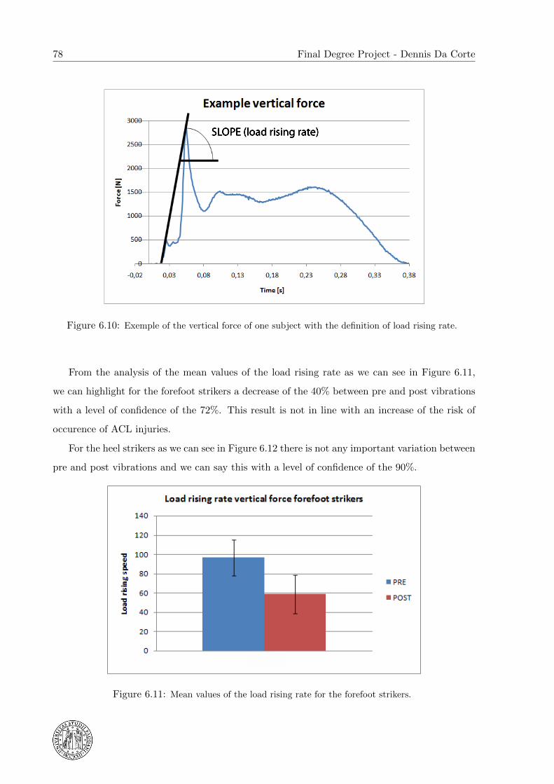
78 Final Degree Project - Dennis Da Corte
Figure 6.10: Exemple of the vertical force of one subject with the definition of load rising rate.
From the analysis of the mean values of the load rising rate as we can see in Figure 6.11,
we can highlight for the forefoot strikers a decrease of the 40% between pre and post vibrations
with a level of confidence of the 72%. This result is not in line with an increase of the risk of
occurence of ACL injuries.
For the heel strikers as we can see in Figure 6.12 there is not any important variation between
pre and post vibrations and we can say this with a level of confidence of the 90%.
Figure 6.11: Mean values of the load rising rate for the forefoot strikers.

Biomechanical analysis of the sidestep cutting maneuver in football players with OpenSim 79
Figure 6.12: Mean values of the load rising rate for the heel strikers.
In Figure 6.13 we can see a summary table of the analysis of the load rising rate (mean
values and standard deviations), with the values of “p” obtained from the t-test.
Figure 6.13: Summary table of the analysis of the load rising rate and the “p” values.
6.3 EMG
Unfortunately the quality of the EMG signals was not very good, so in our analysis an evaluation
of the experimental activations of the muscles was not possible. These data would have been
interesting in order to evaluate the reliability of the numerical simulation (that will be presented
in the following chapter), comparing the experimental activations of the muscles (coming from
the EMG system) with the estimated activations of the muscles (coming from OpenSim).
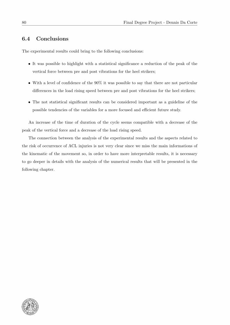
80 Final Degree Project - Dennis Da Corte
6.4 Conclusions
The experimental results could bring to the following conclusions:
• It was possible to highlight with a statistical significance a reduction of the peak of the
vertical force between pre and post vibrations for the heel strikers;
• With a level of confidence of the 90% it was possible to say that there are not particular
differences in the load rising speed between pre and post vibrations for the heel strikers;
• The not statistical significant results can be considered important as a guideline of the
possible tendencies of the variables for a more focused and efficient future study.
An increase of the time of duration of the cycle seems compatible with a decrease of the
peak of the vertical force and a decrease of the load rising speed.
The connection between the analysis of the experimental results and the aspects related to
the risk of occurrence of ACL injuries is not very clear since we miss the main informations of
the kinematic of the movement so, in order to have more interpretable results, it is necessary
to go deeper in details with the analysis of the numerical results that will be presented in the
following chapter.

Biomechanical analysis of the sidestep cutting maneuver in football players with OpenSim 81
Chapter 7
Numerical results and discussion
As we did for the analysis of the experimental results, also for the analysis of the numerical results
the subjects have been split in the two classes (forefoot strikers and heel strikers) according with
the technique of execution of the movement, and two parallel analyses have been done.
7.1 Kinematics
Before starting the treatment of the Inverse Kinematics results coming from OpenSim, these data
have been filtered with a Butterworth low-pass filter of the third order with a cutoff frequency
of 15 Hz.
Let’s present the variables we decided to focus on in order to highlight the possible effects
of the mechanical vibrations on the kinematics of the subjects:
• Maximum knee flexion angle: we expect that if the control on the knee is lower, the angle
of maximum flexion of the knee should be higher.
• Range of motion of knee flexion: we expect that, the worse is the capacity of controlling
the movement of the knee the higher should be this variable. In the literature, this variable
has been identified as directly related to the risk of occurrence of ACL injuries [7].
• Maximum knee abduction angle: this variable corresponds to the minimum negative value
of the knee adduction angle (valgus). The loading in valgus position is the main condition
that brings to ACL injuries, as explained by Koga et al. [9].

82 Final Degree Project - Dennis Da Corte
7.1.1 Maximum knee flexion angle
We can see a comparison of the results of the knee flexion angles for the different subjects in
Figure 7.1 for the forefoot strikers (pre on the left and post on the right) and in Figure 7.2 for
the heel strikers (pre on the left and post on the right).
0 10 20 30 40 50 60 70 80 90 1000
10
20
30
40
50
60
70
80
90
% of time
angl
e [º
]
KNEE FLEXION ANGLE PRE DIFFERENT SUBJECTS
0 10 20 30 40 50 60 70 80 90 1000
10
20
30
40
50
60
70
80
90
% of time
angl
e [º
]
KNEE FLEXION ANGLE POST DIFFERENT SUBJECTS
Figure 7.1: Example of comparison of the knee flexion angles of different subjects for forefoot
strikers pre vibrations (on the left) and post vibrations (on the right).
0 10 20 30 40 50 60 70 80 90 1000
10
20
30
40
50
60
70
80
90
% of time
angl
e [º
]
KNEE FLEXION ANGLE PRE DIFFERENT SUBJECTS
0 10 20 30 40 50 60 70 80 90 1000
10
20
30
40
50
60
70
80
90
% of time
angl
e [º
]
KNEE FLEXION ANGLE POST DIFFERENT SUBJECTS
Figure 7.2: Example of comparison of the knee flexion angles of different subjects for heel
strikers pre vibrations (on the left) and post vibrations (on the right).
In the forefoot strikers class, as we can see in Figure 7.3, there is no significant difference

Biomechanical analysis of the sidestep cutting maneuver in football players with OpenSim 83
between the mean values of the maximum flexion angle between pre and post vibrations, anyway
the “p” value of the t-test is very high (0,893), so this result is not statistically significant.
In the heel strikers class there is an evident increase (∼13◦) of the mean value of the maximum
knee flexion angle between pre and post groups, as we can see in Figure 7.4. Since the “p” value
of the t-test is low (0,015) this result is statistically significant and can be considerd as an evident
consequence of the loose of control due to the mechanical vibrations warming-up.
The standard deviation is similar both between the groups (pre and post) and between the
classes (forefoot strikers and heel strikers).
Figure 7.3: Maximum knee flexion angle for forefoot strikers.

84 Final Degree Project - Dennis Da Corte
Figure 7.4: Maximum knee flexion angle for heel strikers.
7.1.2 Range of motion of the knee flexion
In the forefoot strikers class, as we can see in Figure 7.5, there is no important difference between
the mean values of the range of motion of the flexion angle between pre and post vibrations
and, since the value of “p” from the t-test is very high (0,959), this result is not statistically
significant.
In the heel strikers class, there is an evident increase (∼14◦) in the mean value of the range of
motion of the knee flexion angle between the pre and the post vibrations trials as we can see in
Figure 6.6. Since the “p” value is very low (0,010), this result is statistically significant and can
be considered as a direct consequence of the loose of control of the knee due to the mechanical
vibrations warming up. We can moreover observe a reduction of the standard deviation between
the pre and the post group, a tendency similar to the one showed for the time of duration of the
cycle.
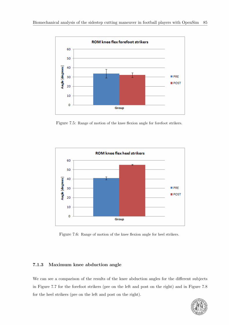
Biomechanical analysis of the sidestep cutting maneuver in football players with OpenSim 85
Figure 7.5: Range of motion of the knee flexion angle for forefoot strikers.
Figure 7.6: Range of motion of the knee flexion angle for heel strikers.
7.1.3 Maximum knee abduction angle
We can see a comparison of the results of the knee abduction angles for the different subjects
in Figure 7.7 for the forefoot strikers (pre on the left and post on the right) and in Figure 7.8
for the heel strikers (pre on the left and post on the right).

86 Final Degree Project - Dennis Da Corte
0 10 20 30 40 50 60 70 80 90 100−10
−5
0
5
10
15
20
% of time
angl
e [º
]
KNEE ABDUCTION ANGLE PRE DIFFERENT SUBJECTS
0 10 20 30 40 50 60 70 80 90 100−10
−5
0
5
10
15
20
% of time
angl
e [º
]
KNEE ABDUCTION ANGLE POST DIFFERENT SUBJECTS
Figure 7.7: Example of comparison of the knee abduction angles of different subjects for
forefoot strikers pre vibrations (on the left) and post vibrations (on the right).
0 10 20 30 40 50 60 70 80 90 100−10
−5
0
5
10
15
20
% of time
angl
e [º
]
KNEE ABDUCTION ANGLE PRE DIFFERENT SUBJECTS
0 10 20 30 40 50 60 70 80 90 100−10
−5
0
5
10
15
20
% of time
angl
e [º
]
KNEE ABDUCTION ANGLE POST DIFFERENT SUBJECTS
Figure 7.8: Example of comparison of the knee abduction angles of different subjects for heel
strikers pre vibrations (on the left) and post vibrations (on the right).
For the forefoot strikers class, as we can see in Figure 7.9, in the pre group the abduction was
not reached so, according with the convention of sign adopted, the mean value of the maximum
abduction angle is negative. In the post group it is possible to observe a very small value of
abduction; this is not important in absolute terms but it is significant if compared to the value
obtained in the pre vibrations group. The “p” value of the t-test is not very high (0,085) so this
result can be considered statistically significant with a level of confidence of the 91%.
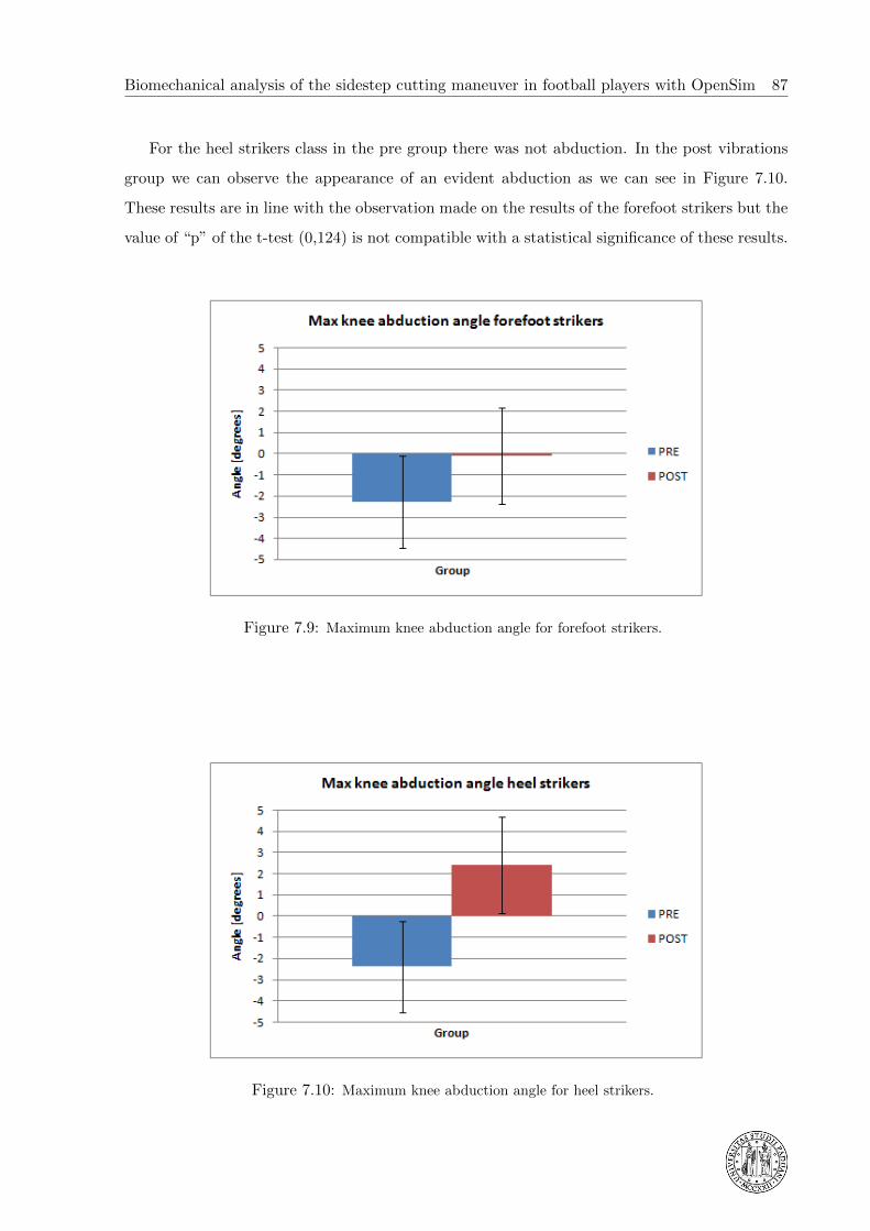
Biomechanical analysis of the sidestep cutting maneuver in football players with OpenSim 87
For the heel strikers class in the pre group there was not abduction. In the post vibrations
group we can observe the appearance of an evident abduction as we can see in Figure 7.10.
These results are in line with the observation made on the results of the forefoot strikers but the
value of “p” of the t-test (0,124) is not compatible with a statistical significance of these results.
Figure 7.9: Maximum knee abduction angle for forefoot strikers.
Figure 7.10: Maximum knee abduction angle for heel strikers.
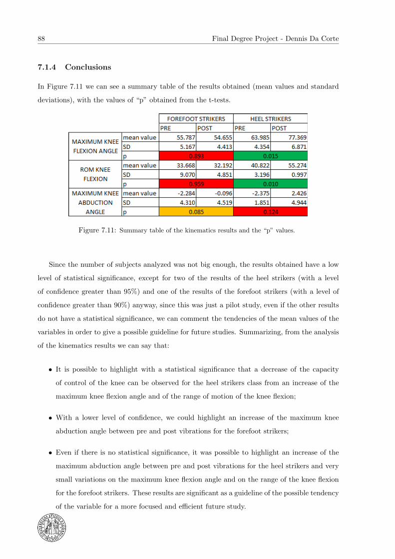
88 Final Degree Project - Dennis Da Corte
7.1.4 Conclusions
In Figure 7.11 we can see a summary table of the results obtained (mean values and standard
deviations), with the values of “p” obtained from the t-tests.
Figure 7.11: Summary table of the kinematics results and the “p” values.
Since the number of subjects analyzed was not big enough, the results obtained have a low
level of statistical significance, except for two of the results of the heel strikers (with a level
of confidence greater than 95%) and one of the results of the forefoot strikers (with a level of
confidence greater than 90%) anyway, since this was just a pilot study, even if the other results
do not have a statistical significance, we can comment the tendencies of the mean values of the
variables in order to give a possible guideline for future studies. Summarizing, from the analysis
of the kinematics results we can say that:
• It is possible to highlight with a statistical significance that a decrease of the capacity
of control of the knee can be observed for the heel strikers class from an increase of the
maximum knee flexion angle and of the range of motion of the knee flexion;
• With a lower level of confidence, we could highlight an increase of the maximum knee
abduction angle between pre and post vibrations for the forefoot strikers;
• Even if there is no statistical significance, it was possible to highlight an increase of the
maximum abduction angle between pre and post vibrations for the heel strikers and very
small variations on the maximum knee flexion angle and on the range of the knee flexion
for the forefoot strikers. These results are significant as a guideline of the possible tendency
of the variable for a more focused and efficient future study.
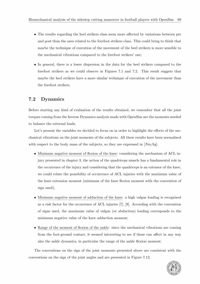
Biomechanical analysis of the sidestep cutting maneuver in football players with OpenSim 89
• The results regarding the heel strikers class seem more affected by variations between pre
and post than the ones related to the forefoot strikers class. This could bring to think that
maybe the technique of execution of the movement of the heel strikers is more sensible to
the mechanical vibrations compared to the forefoot strikers’ one;
• In general, there is a lower dispersion in the data for the heel strikers compared to the
forefoot strikers as we could observe in Figures 7.1 and 7.2. This result suggets that
maybe the heel strikers have a more similar technique of execution of the movement than
the forefoot strikers.
7.2 Dynamics
Before starting any kind of evaluation of the results obtained, we remember that all the joint
torques coming from the Inverse Dynamics analysis made with OpenSim are the moments needed
to balance the external loads.
Let’s present the variables we decided to focus on in order to highlight the effects of the me-
chanical vibrations on the joint moments of the subjects. All these results have been normalized
with respect to the body mass of the subjects, so they are expressed in [Nm/kg]:
• Minimum negative moment of flexion of the knee: considering the mechanism of ACL in-
jury presented in chapter 3, the action of the quadriceps muscle has a fundamental role in
the occurrence of the injury and considering that the quadriceps is an extensor of the knee,
we could relate the possibility of occurrence of ACL injuries with the maximum value of
the knee extension moment (minimum of the knee flexion moment with the convention of
sign used);
• Minimum negative moment of adduction of the knee: a high valgus loading is recognized
as a risk factor for the occurrence of ACL injuries [7], [9]. According with the convention
of signs used, the maximum value of valgus (or abduction) loading corresponds to the
minimum negative value of the knee adduction moment;
• Range of the moment of flexion of the ankle: since the mechanical vibrations are coming
from the foot-ground contact, it seemed interesting to see if those can affect in any way
also the ankle dynamics, in particular the range of the ankle flexion moment.
The conventions on the sign of the joint moments presented above are consistent with the
conventions on the sign of the joint angles and are presented in Figure 7.12.

90 Final Degree Project - Dennis Da Corte
Figure 7.12: Convention on the definition of the signs of the knee flexion moment (on the left), of the
knee adduction moment (in the middle) and of ankle flexion moment (on the right).
7.2.1 Minimum negative knee flexion moment
In Figure 7.13 we can see an example of plot of the knee flexion moment, in order to clarify the
convention of sign adopted and the meaning of the different peaks highlighted.
Figure 7.13: Example of knee flexion moment with the convention of sign adopted and the meaning of
the peaks.
We can see a comparison of the results of the knee flexion moment for the different subjects
in Figure 7.14 for the forefoot strikers (pre on the left and post on the right) and in Figure 7.15

Biomechanical analysis of the sidestep cutting maneuver in football players with OpenSim 91
for the heel strikers (pre on the left and post on the right).
0 10 20 30 40 50 60 70 80 90 100
−4
−3
−2
−1
0
1
2
3
% of time
mom
ent/b
ody
mas
s [N
m/k
g]
KNEE FLEXION MOMENT PRE DIFFERENT SUBJECTS
0 10 20 30 40 50 60 70 80 90 100
−4
−3
−2
−1
0
1
2
3
% of time
mom
ent/b
ody
mas
s [N
m/k
g]
KNEE FLEXION MOMENT POST DIFFERENT SUBJECTS
Figure 7.14: Comparison of the knee flexion moments of different subjects for forefoot strikers
pre vibrations (on the left) and post vibrations (on the right).
0 10 20 30 40 50 60 70 80 90 100
−4
−3
−2
−1
0
1
2
3
% of time
mom
ent/b
ody
mas
s [N
m/k
g]
KNEE FLEXION MOMENT PRE DIFFERENT SUBJECTS
0 10 20 30 40 50 60 70 80 90 100
−4
−3
−2
−1
0
1
2
3
% of time
mom
ent/b
ody
mas
s [N
m/k
g]
KNEE FLEXION MOMENT POST DIFFERENT SUBJECTS
Figure 7.15: Comparison of the knee flexion moments of different subjects for heel strikers pre
vibrations (on the left) and post vibrations (on the right).
For the forefoot strikers, as we can see in Figure 7.16 there is an important decrease (around
30%) of the mean value of the minimum knee flexion moment between pre and post vibrations.
For the heel strikers, as we can see in Figure 7.17, it is not possible to appreciate any partic-
ularvariation of the mean value of the minimum knee flexion moment between pre and post
vibrations. For both the classes the value of “p” of the t-test is high (0,191 for the forefoot

92 Final Degree Project - Dennis Da Corte
strikers and 0,610 for the heel strikers) so the results are not statistically significant.
The tendency for the forefoot strikers is in line with an increase of the risk of occurrence of
ACL injuries, but we do not have the statistical significance of the results.
Figure 7.16: Minimum knee flexion moment for forefoot strikers.
Figure 7.17: Minimum knee flexion moment for heel strikers.
The standard deviation between forefoot strikers and heel strikers for both the classes is
similar, so the dispersion of the data is quite similar for this variable, as we could see in Figures
7.14 and 7.15.
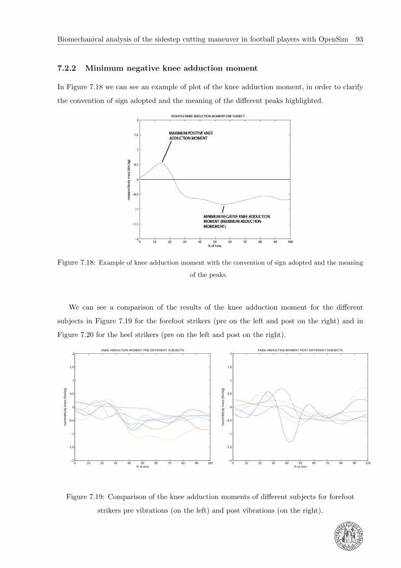
Biomechanical analysis of the sidestep cutting maneuver in football players with OpenSim 93
7.2.2 Minimum negative knee adduction moment
In Figure 7.18 we can see an example of plot of the knee adduction moment, in order to clarify
the convention of sign adopted and the meaning of the different peaks highlighted.
Figure 7.18: Example of knee adduction moment with the convention of sign adopted and the meaning
of the peaks.
We can see a comparison of the results of the knee adduction moment for the different
subjects in Figure 7.19 for the forefoot strikers (pre on the left and post on the right) and in
Figure 7.20 for the heel strikers (pre on the left and post on the right).
0 10 20 30 40 50 60 70 80 90 100−2
−1.5
−1
−0.5
0
0.5
1
1.5
2
% of time
mom
ent/b
ody
mas
s [N
m/k
g]
KNEE ABDUCTION MOMENT PRE DIFFERENT SUBJECTS
0 10 20 30 40 50 60 70 80 90 100−2
−1.5
−1
−0.5
0
0.5
1
1.5
2
% of time
mom
ent/b
ody
mas
s [N
m/k
g]
KNEE ABDUCTION MOMENT POST DIFFERENT SUBJECTS
Figure 7.19: Comparison of the knee adduction moments of different subjects for forefoot
strikers pre vibrations (on the left) and post vibrations (on the right).

94 Final Degree Project - Dennis Da Corte
0 10 20 30 40 50 60 70 80 90 100−2
−1.5
−1
−0.5
0
0.5
1
1.5
2
% of time
mom
ent/b
ody
mas
s [N
m/k
g]
KNEE ABDUCTION MOMENT PRE DIFFERENT SUBJECTS
0 10 20 30 40 50 60 70 80 90 100−2
−1.5
−1
−0.5
0
0.5
1
1.5
2
% of time
mom
ent/b
ody
mas
s [N
m/k
g]
KNEE ABDUCTION MOMENT POST DIFFERENT SUBJECTS
Figure 7.20: Comparison of the knee adduction moments of different subjects for heel strikers
pre vibrations (on the left) and post vibrations (on the right).
For the forefoot strikers, as we can see in Figure 7.21, we can observe an important increase
of the mean value of the minimum knee adduction moment (around 30%) between pre and post
vibrations. This result is not in line with an increase of the risk of occurrence of ACL injuries.
For the heel strikers, as we can see in Figures 7.22, there is an important decrease (around
20%) of the mean value of the minimum knee flexion moment between pre and post vibrations.
This result seems in line with an increase of the risk of occurrence of ACL injuries.
For both the classes the value of “p” of the t-test is high (0,322 for the forefoot strikers and
0,796 for the heel strikers) so the results are not statistically significant.

Biomechanical analysis of the sidestep cutting maneuver in football players with OpenSim 95
Figure 7.21: Minimum knee adduction moment for forefoot strikers.
Figure 7.22: Minimum knee adduction moment for heel strikers.
7.2.3 Range of the moment of flexion of the ankle
We can see a comparison of the results of the ankle flexion moment for the different subjects in
Figure 7.23 for the forefoot strikers (pre on the left and post on the right) and in Figure 7.24
for the heel strikers (pre on the left and post on the right).

96 Final Degree Project - Dennis Da Corte
0 10 20 30 40 50 60 70 80 90 100
−4
−3
−2
−1
0
1
2
% of time
mom
ent/b
ody
mas
s [N
m/k
g]
ANKLE FLEXION MOMENT PRE DIFFERENT SUBJECTS
0 10 20 30 40 50 60 70 80 90 100
−4
−3
−2
−1
0
1
2
% of time
mom
ent/b
ody
mas
s [N
m/k
g]
ANKLE FLEXION MOMENT POST DIFFERENT SUBJECTS
Figure 7.23: Comparison of the ankle flexion moments of different subjects for forefoot strikers
pre vibrations (on the left) and post vibrations (on the right).
0 10 20 30 40 50 60 70 80 90 100
−4
−3
−2
−1
0
1
2
% of time
mom
ent/b
ody
mas
s [N
m/k
g]
ANKLE FLEXION MOMENT PRE DIFFERENT SUBJECTS
0 10 20 30 40 50 60 70 80 90 100
−4
−3
−2
−1
0
1
2
% of time
mom
ent/b
ody
mas
s [N
m/k
g]
ANKLE FLEXION MOMENT POST DIFFERENT SUBJECTS
Figure 7.24: Comparison of the ankle flexion moments of different subjects for heel strikers pre
vibrations (on the left) and post vibrations (on the right).
For the forefoot strikers class, as we can see in Figure 7.25, the range of the ankle flexion
moment increased of more or less the 20% between pre and post. This could be considered as
an evident effect of the mechanical vibrations warming-up on the ankle flexion dynamics.
In the heel strikers class as we can see in Figure 7.26, the range of the ankle flexion moment
increased of more or less the 40% between pre and post. This could be considered as an evident
effect of the mechanical vibrations warming-up on the ankle flexion dynamics.

Biomechanical analysis of the sidestep cutting maneuver in football players with OpenSim 97
The values of “p” calculated trough the t-test are lower than 0,1 (0,085 for the forefoot
strikers and 0,079 for the heel strikers), so the statistical reliability of the comparisons is good
with a level of confidence greater than 90%.
Figure 7.25: Range of the ankle flexion moment for forefoot strikers.
Figure 7.26: Range of the ankle flexion moment for heel strikers.
7.2.4 Conclusions
In Figure 7.27 we can see a summary table of the results obtained (mean values and standard
deviations), with the values of “p” obtained from the t-tests.
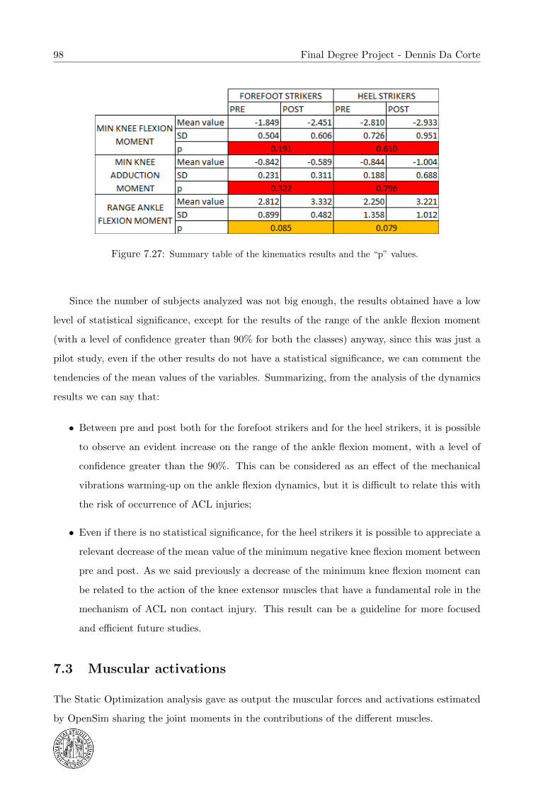
98 Final Degree Project - Dennis Da Corte
Figure 7.27: Summary table of the kinematics results and the “p” values.
Since the number of subjects analyzed was not big enough, the results obtained have a low
level of statistical significance, except for the results of the range of the ankle flexion moment
(with a level of confidence greater than 90% for both the classes) anyway, since this was just a
pilot study, even if the other results do not have a statistical significance, we can comment the
tendencies of the mean values of the variables. Summarizing, from the analysis of the dynamics
results we can say that:
• Between pre and post both for the forefoot strikers and for the heel strikers, it is possible
to observe an evident increase on the range of the ankle flexion moment, with a level of
confidence greater than the 90%. This can be considered as an effect of the mechanical
vibrations warming-up on the ankle flexion dynamics, but it is difficult to relate this with
the risk of occurrence of ACL injuries;
• Even if there is no statistical significance, for the heel strikers it is possible to appreciate a
relevant decrease of the mean value of the minimum negative knee flexion moment between
pre and post. As we said previously a decrease of the minimum knee flexion moment can
be related to the action of the knee extensor muscles that have a fundamental role in the
mechanism of ACL non contact injury. This result can be a guideline for more focused
and efficient future studies.
7.3 Muscular activations
The Static Optimization analysis gave as output the muscular forces and activations estimated
by OpenSim sharing the joint moments in the contributions of the different muscles.

Biomechanical analysis of the sidestep cutting maneuver in football players with OpenSim 99
The comparison has been made between the muscular activations estimated for the trials
pre and post vibrations in order to see if it was possible to highlight any interesting effect due
to the mechanical vibrations warming-up. Two different kind of analysis have been made:
• A qualitative analysis looking at the shape of the curves and the peak values;
• A quantitative analysis looking at the value of the integral of the curve of the activation
of the muscle.
The integral of the curve of activation of a muscle represents the total amount of energy
generated during the execution of the movement and it is proportional to the average level of
activation of the muscle. The value of the integral of the curve has been calculated with Matlab
using the trapezoidal numerical integration with a resolution of 1%; since the two axes are
expressed in percentage, the integral is dimensionless and always lower than 10000. In Figure
7.28 we can see the graphical definition of the integral of a curve of activation of a muscle.
Figure 7.28: Graphical definition of the integral of a curve of activation of a muscle.
The muscles we decided to analyze are the same muscles collected with the EMG system
(vastus lateralis, biceps femoris, rectus anterior, semitendinosus and soleus). In this way, in
future, it will be possible to make a parallel analysis based on the activations coming from the
EMG data and see if it is possible to validate the simulations.

100 Final Degree Project - Dennis Da Corte
Soleus:
This is one of the main plantar flexors of the ankle. The activation of this muscle presents
the most evident differences between pre and post vibrations. For all the subjects it is possible
to observe an increase of the maximum value of activation between the pre and the post group.
This result is perfectly in accordance with the results of the Inverse Dynamics analysis: in fact a
reduction of the minimum ankle flexion moment was highlighted between pre and post vibrations
and this suggests an increase of the activity of the muscles responsible of the plantar flexion of
the ankle. The trend of the activation is always growing in the time for all the subjects and for
all the trials, with the peak of activation very close to the ending of the eccentric phase of the
movement.
For the heel strikers we can observe a flat zone on the activation of the soleus near the initial
contact of the foot with the floor. Since these subjects are landing with the heel, in the first
part of the movement the moment of plantar flexion of the ankle is smaller than for the forefoot
strikers, since the toe is not touching the ground yet.
In Figure 7.36 we can observe the curves of the activation of this muscle for the forefoot
strikers and for the heel strikers.
The analysis of the integrals of the plots highlighted an increase of the area under the plots
between pre and post vibrations both for the forefoot strikers (with a level of confidence of the
97%) and for the heel strikers (with a level of confidence of the 75%). The area under the plots
is representative of the level of activation of the muscle during the execution of the movement,
so the soleus is more activated post vibrations than pre. The mean values, standard deviations
and “p” values coming from the t-test for the soleus can be seen in Figure 7.29.
Figure 7.29: Summary table of the integral analysis of the activation of the soleus.
Long head of the biceps femoris:
This is a bi-articular muscle, responsible mainly for the flexion of the knee and for the
extension of the hip. For this muscle it is possible to observe a reduction of the maximum values

Biomechanical analysis of the sidestep cutting maneuver in football players with OpenSim 101
of activation between pre and post vibrations, as we can see in Figure 7.37.
The shape of most of the activation plots of this muscle, follows a wave with two main peaks
and two main valleys.
The analysis of the integrals of the plots highlighted a decrease of the area under the plots
between pre and post vibrations both for the forefoot strikers (with a level of confidence of the
99%) and for the heel strikers (with a level of confidence of the 88%). The area under the plots is
representative of the level of activation of the muscle during the execution of the movement, so
the long head of the biceps femoris is less activated post vibrations than pre. The mean values,
standard deviations and “p” values coming from the t-test for the long head of the biceps femoris
can be seen in Figure 7.30.
Figure 7.30: Summary table of the integral analysis of the activation of the long head of the biceps
femoris.
Short head of the biceps femoris:
This is a muscle responsible for the flexion of the knee. As we can see in Figure 7.38, in the
activation of this muscle it is not possible to observe a unique trend of variation beetween pre
and post vibrations.
We can observe that the average level of activation of this muscle is always lower than the
one of the long head of the biceps femoris.
The analysis of the integrals of the plots highlighted a decrease of the area under the plots
between pre and post vibrations both for the forefoot strikers (with a level of confidence of the
93%) and for the heel strikers (with a level of confidence of the 93%). The area under the plots
is representative of the level of activation of the muscle during the execution of the movement,
so the short head of the biceps femoris is less activated post vibrations than pre. The mean
values, standard deviations and “p” values coming from the t-test for the short head of the
biceps femoris can be seen in Figure 7.31.

102 Final Degree Project - Dennis Da Corte
Figure 7.31: Summary table of the integral analysis of the activation of the short head of the biceps
femoris.
Semitendinosus:
This is a biarticular muscle responsible mainly for the flexion of the knee. For most of the
subjects, it is possible to observe an increase on the maximum value of activation of this muscle
between pre and post vibrations.
The maximum values of activation reached for two of the three heel strikers, are higher than
the ones reached by the forefoot strikers. This suggests that maybe the technique of execution
of the movement of the heel strikers requires a more important contribution of this muscle.
The plots for comparing the activation of the semitendinosus muscle among the trials can
be seen in Figure 7.39.
As we can observe in Figure 7.32 it is not possible to observe any common tendency of the
integral of the activation of this muscle and the level of confidence of these results is very low.
Figure 7.32: Summary table of the integral analysis of the activation of semitendinosus.
Vastus lateralis: This muscle is responsible for the extension of the knee. As we can see in
Figure 7.40, the maximum value of the activation of this muscle, decreases or stays more or less
constant between pre and post vibrations for all the subjects, maintaining also a very similar
shape of the curves.
The plots of the activation of this muscle present almost for all the subjects, a flat zone
at the beginning, a ramp-up and than another almost flat zone at the end of the cycle. This
suggests that the different way of execution of the movement between forefoot strikers and heel

Biomechanical analysis of the sidestep cutting maneuver in football players with OpenSim 103
strikers, does not affect significantly the activation patten of this muscle.
The analysis of the integrals of the plots highlighted a decrease of the area under the plots
between pre and post vibrations both for the forefoot strikers (with a level of confidence of the
93%) and for the heel strikers (with a level of confidence of the 91%). The area under the plots
is representative of the level of activation of the muscle during the execution of the movement,
so the vastus lateralis is less activated post vibrations than pre. The mean values, standard
deviations and “p” values coming from the t-test for the vastus lateralis can be seen in Figure
7.33.
Figure 7.33: Summary table of the integral analysis of the activation of the vastus lateralis.
Rectus anterior:
This is a biarticular muscle responsible for the extension of the knee. The activation of this
muscle, both in the pre and in the post vibrations, is very low for almost all the subjects analyzed
as we can see in Figure 7.41. This could seem in disaccordance with the results of the Inverse
Dynamics analysis, where we could see a quite low minimum in the knee flexion moments (high
knee extension moments).
In order to clarify this question, in Figure 7.35 we can see in red the total knee flexion
moment and in other colours the contribution of each muscle to this moment (calculated as
force of the muscle multiplied by its lever arm). We can see that the contribution of the rectus
anterior to the extension moment is negligible if compared with the contribution of the vastus
lateralis (in violet). So we can conclude that the activation of the rectus anterior is very low
because the cknee extension moment is exerted mainly by the vastus lateralis.
The analysis of the integrals of the plots highlighted an increase of the area under the plots
between pre and post vibrations both for the forefoot strikers and for the heel strikers but with
a very low level of confidence (lower than the 60%). The area under the plots is representative
of the level of activation of the muscle during the execution of the movement, so the rectus
anterior is more activated post vibrations than pre. The mean values, standard deviations and
“p” values coming from the t-test for the rectus anterior can be seen in Figure 7.34.

104 Final Degree Project - Dennis Da Corte
Figure 7.34: Summary table of the integral analysis of the activation of the rectus anterior.
-150
-100
-50
0
50
100
0 0,05 0,1 0,15 0,2
mo
me
nt
[Nm
]
!me [s]
Contribu!on Knee Flexion Moment
semimem_r
semiten_r
bifemlh_r
rect_fem_r
vas_int_r
vas_lat_r
Knee flexion moment
Figure 7.35: Example of the contribution of each muscle to the knee flexion moment for one of the
forefoot strikers.

Biomechanical analysis of the sidestep cutting maneuver in football players with OpenSim 105
0 10 20 30 40 50 60 70 80 90 1000
50
100SOLEUS FOREFOOT STRIKERS
% o
f act
ivat
ion
0 10 20 30 40 50 60 70 80 90 1000
50
100
% o
f act
ivat
ion
0 10 20 30 40 50 60 70 80 90 1000
50
100
% o
f act
ivat
ion
0 10 20 30 40 50 60 70 80 90 1000
50
100
% o
f act
ivat
ion
0 10 20 30 40 50 60 70 80 90 1000
50
100
% o
f act
ivat
ion
0 10 20 30 40 50 60 70 80 90 1000
50
100
% of time
% o
f act
ivat
ion
PREPOST
0 10 20 30 40 50 60 70 80 90 1000
50
100SOLEUS HEEL STRIKERS
% o
f act
ivat
ion
0 10 20 30 40 50 60 70 80 90 1000
50
100
% o
f act
ivat
ion
0 10 20 30 40 50 60 70 80 90 1000
50
100
% of time
% o
f act
ivat
ion
PREPOST
Figure 7.36: Comparison of the activation of the soleus for forefoot strikers (above) and heel
strikers (below) pre vibrations and post vibrations.

106 Final Degree Project - Dennis Da Corte
0 10 20 30 40 50 60 70 80 90 1000
50
100BICEPS FEMORIS1 FOREFOOT STRIKERS
% o
f act
ivat
ion
0 10 20 30 40 50 60 70 80 90 1000
50
100
% o
f act
ivat
ion
0 10 20 30 40 50 60 70 80 90 1000
50
100
% o
f act
ivat
ion
0 10 20 30 40 50 60 70 80 90 1000
50
100
% o
f act
ivat
ion
0 10 20 30 40 50 60 70 80 90 1000
50
100
% o
f act
ivat
ion
0 10 20 30 40 50 60 70 80 90 1000
50
100
% of time
% o
f act
ivat
ion
PREPOST
0 10 20 30 40 50 60 70 80 90 1000
50
100BICEPS FEMORIS1 HEEL STRIKERS
% o
f act
ivat
ion
0 10 20 30 40 50 60 70 80 90 1000
50
100
% o
f act
ivat
ion
0 10 20 30 40 50 60 70 80 90 1000
50
100
% of time
% o
f act
ivat
ion
PREPOST
Figure 7.37: Comparison of the activation of the long head of the biceps femoris for forefoot
strikers (above) and heel strikers (below) pre vibrations and post vibrations.
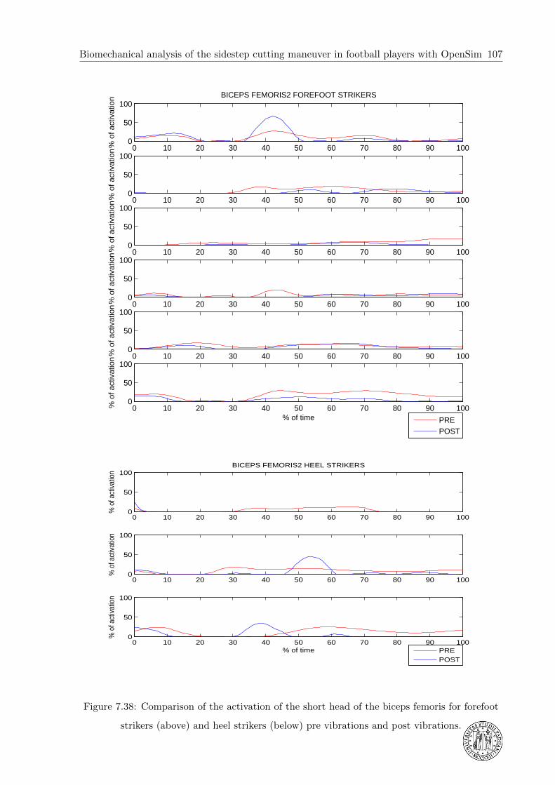
Biomechanical analysis of the sidestep cutting maneuver in football players with OpenSim 107
0 10 20 30 40 50 60 70 80 90 1000
50
100BICEPS FEMORIS2 FOREFOOT STRIKERS
% o
f act
ivat
ion
0 10 20 30 40 50 60 70 80 90 1000
50
100
% o
f act
ivat
ion
0 10 20 30 40 50 60 70 80 90 1000
50
100
% o
f act
ivat
ion
0 10 20 30 40 50 60 70 80 90 1000
50
100
% o
f act
ivat
ion
0 10 20 30 40 50 60 70 80 90 1000
50
100
% o
f act
ivat
ion
0 10 20 30 40 50 60 70 80 90 1000
50
100
% of time
% o
f act
ivat
ion
PREPOST
0 10 20 30 40 50 60 70 80 90 1000
50
100BICEPS FEMORIS2 HEEL STRIKERS
% o
f act
ivat
ion
0 10 20 30 40 50 60 70 80 90 1000
50
100
% o
f act
ivat
ion
0 10 20 30 40 50 60 70 80 90 1000
50
100
% of time
% o
f act
ivat
ion
PREPOST
Figure 7.38: Comparison of the activation of the short head of the biceps femoris for forefoot
strikers (above) and heel strikers (below) pre vibrations and post vibrations.

108 Final Degree Project - Dennis Da Corte
0 10 20 30 40 50 60 70 80 90 1000
50
100SEMITENDINOSUS FOREFOOT STRIKERS
% o
f act
ivat
ion
0 10 20 30 40 50 60 70 80 90 1000
50
100
% o
f act
ivat
ion
0 10 20 30 40 50 60 70 80 90 1000
50
100
% o
f act
ivat
ion
0 10 20 30 40 50 60 70 80 90 1000
50
100
% o
f act
ivat
ion
0 10 20 30 40 50 60 70 80 90 1000
50
100
% o
f act
ivat
ion
0 10 20 30 40 50 60 70 80 90 1000
50
100
% of time
% o
f act
ivat
ion
PREPOST
0 10 20 30 40 50 60 70 80 90 1000
50
100SEMITENDINOSUS HEEL STRIKERS
% o
f act
ivat
ion
0 10 20 30 40 50 60 70 80 90 1000
50
100
% o
f act
ivat
ion
0 10 20 30 40 50 60 70 80 90 1000
50
100
% of time
% o
f act
ivat
ion
PREPOST
Figure 7.39: Comparison of the activation of the semitendinosus for forefoot strikers (above)
and heel strikers (below) pre vibrations and post vibrations.

Biomechanical analysis of the sidestep cutting maneuver in football players with OpenSim 109
0 10 20 30 40 50 60 70 80 90 1000
50
100VASTUS LATERALIS FOREFOOT STRIKERS
% o
f act
ivat
ion
0 10 20 30 40 50 60 70 80 90 1000
50
100
% o
f act
ivat
ion
0 10 20 30 40 50 60 70 80 90 1000
50
100
% o
f act
ivat
ion
0 10 20 30 40 50 60 70 80 90 1000
50
100
% o
f act
ivat
ion
0 10 20 30 40 50 60 70 80 90 1000
50
100
% o
f act
ivat
ion
0 10 20 30 40 50 60 70 80 90 1000
50
100
% of time
% o
f act
ivat
ion
PREPOST
0 10 20 30 40 50 60 70 80 90 1000
50
100VASTUS LATERALIS HEEL STRIKERS
% o
f act
ivat
ion
0 10 20 30 40 50 60 70 80 90 1000
50
100
% o
f act
ivat
ion
0 10 20 30 40 50 60 70 80 90 1000
50
100
% of time
% o
f act
ivat
ion
PREPOST
Figure 7.40: Comparison of the activation of the vastus lateralis for forefoot strikers (above)
and heel strikers (below) pre vibrations and post vibrations.

110 Final Degree Project - Dennis Da Corte
0 10 20 30 40 50 60 70 80 90 1000
50
100RECTUS ANTERIOR FOREFOOT STRIKERS
% o
f act
ivat
ion
0 10 20 30 40 50 60 70 80 90 1000
50
100
% o
f act
ivat
ion
0 10 20 30 40 50 60 70 80 90 1000
50
100
% o
f act
ivat
ion
0 10 20 30 40 50 60 70 80 90 1000
50
100
% o
f act
ivat
ion
0 10 20 30 40 50 60 70 80 90 1000
50
100
% o
f act
ivat
ion
0 10 20 30 40 50 60 70 80 90 1000
50
100
% of time
% o
f act
ivat
ion
PREPOST
0 10 20 30 40 50 60 70 80 90 1000
50
100RECTUS ANTERIOR HEEL STRIKERS
% o
f act
ivat
ion
0 10 20 30 40 50 60 70 80 90 1000
50
100
% o
f act
ivat
ion
0 10 20 30 40 50 60 70 80 90 1000
50
100
% of time
% o
f act
ivat
ion
PREPOST
Figure 7.41: Comparison of the activation of the rectus anterior for forefoot strikers (above)
and heel strikers (below) pre vibrations and post vibrations.
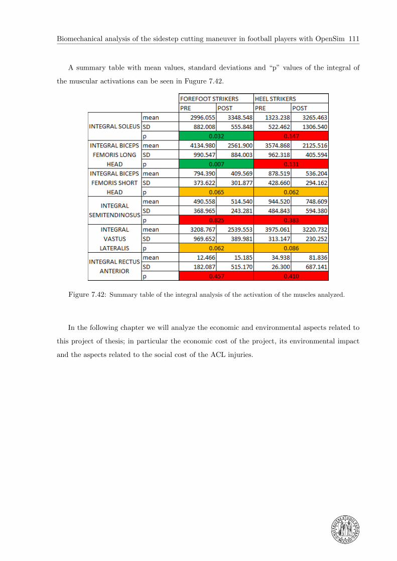
Biomechanical analysis of the sidestep cutting maneuver in football players with OpenSim 111
A summary table with mean values, standard deviations and “p” values of the integral of
the muscular activations can be seen in Fugure 7.42.
Figure 7.42: Summary table of the integral analysis of the activation of the muscles analyzed.
In the following chapter we will analyze the economic and environmental aspects related to
this project of thesis; in particular the economic cost of the project, its environmental impact
and the aspects related to the social cost of the ACL injuries.

112 Final Degree Project - Dennis Da Corte

Biomechanical analysis of the sidestep cutting maneuver in football players with OpenSim 113
Chapter 8
Economic and environmental aspects
8.1 Economic cost of the project
The economic cost of this project is mainly represented by:
• The depreciation of the instrumentation and the software used during the project;
• The cost of the time of working of all the people involved in it;
• The cost of the consumable material.
The equipment used during the project is composed by:
• The instrumentation of the laboratory of the CAR composed by the motion capture system
(including the computer and the software licenses), the force platform, the EMG system
and the mechanical vibrations machine;
• The computer of the office of the ETSEIB used by the student.
For the instrumentation of the laboratory of the CAR we can estimate an average operating
life of 8 years, considering a utilization of 45 weeks per year and for a weekly use of 10 hours.
The total number of operating hours of the equipment is 3600 hours.
For the computer of the ETSEIB we can estimate an average operating life of 5 years,
considering a utilization of 45 weeks per year and a weekly use of 50 hours. The total number
of operating hours of the computer is 11250.
The effective use of the lab equipment to make 9 motion captures has been 18 hours. Since
the motion capture system is a visible light video system and not an infrared video system, the
114 Final Degree Project - Dennis Da Corte
process of reconstruction of the trajectories of the markers and preparation of the data to feed
OpenSim have been quite long and can be estimated in 2 hours for each subject yielding a total
of 18 hours.
The student spent 630 hours working with the computer of the office in order to find infor-
mation and bibliography, to study the operation of the software used, to process the data, to
analyze the results and to write the final report of the master thesis. The calculation of the
depreciation of the equipment is resumed in Table 7.1 and the total cost of depreciation is 363,90
e.
Considering the cost of working of the people involved in the project we have to distinguish
between the work of the student and the work of the people at the laboratory.
The execution of the tests has been made by four people, two of them were students and two
of them were internal employees of the CAR. The salary recommended by the ETSEIB for an
engineering student is of 8 e/h and the salary of an employee of the CAR is 16 e/h. The total
cost of the work of the people involved in the execution of the tests can be quantified in:
8e/h · 18h+ 16e/h · 18h = 432e (8.1)
The preparation of the data to feed OpenSim has been made by one student and the cost of
his work can be quantified in:
8e/h · 18h = 144e (8.2)
For the total time of 630 hours, the cost of the work of the student can be quantified in:
8e/h · 630h = 5040e (8.3)
So, the total labor cost is:
432e+ 144e+ 5040e = 5616e (8.4)
We decided to neglect the cost due to the electricity consumption, because the use of elec-
tricity hasn’t involved any significant increase on the consumption at CAR and ETSEIB.
We have to consider also the cost of the consumable material used during the execution of
the tests (double side tape, disposable electrodes, material for preparing the skin for the EMG,
etc.) that can be quantified in 60 e.

Biomechanical analysis of the sidestep cutting maneuver in football players with OpenSim 115
Equ
ipm
ent
Tota
lco
st[e
]O
per
ati
ng
life
[h]
Dep
reci
atio
np
erh
our
[e/h
]T
ime
of
use
[h]
Cos
tof
dep
reci
atio
n[e
]
Moti
on
cap
ture
syst
em
Pea
kM
otus
9.2.
0+
com
pu
ter
16000
3600
4,4
3616
0,00
For
cep
latf
orm
Kis
tler
928
1B
12000
3600
3,33
1860,
00
EM
Gsy
stem
Meg
aW
BA
16200
3600
4,5
1881,
00
Mec
han
ical
vib
rati
ons
mach
ine
ViB
alan
ce2500
3600
0,69
1812,
50
Com
pu
ter
900
1125
00,
0863
050,
40
TO
TA
L[e
]
363,9
0
Tab
le7.
1:C
alcu
lati
on
of
the
dep
reci
ati
on
of
the
equ
ipm
ent.

116 Final Degree Project - Dennis Da Corte
Summing all the contributions of cost, we can say that the total cost of the execution of the
project has been:
363, 90e+ 5616e+ 60e = 6039, 90e (8.5)
8.2 Environmental impact of the project
The environmental impact of this project is reduced because no significant waste has been
generated during it. The only waste we can talk about is the double side tape used to attach
the markers on the skin and the disposable electrodes. We can quantify the double side tape
consummate in 3 cm for each marker for 12 markers for each subject and for 10 subjects for a
total of 360 cm of tape. The number of disposable electrodes used during the execution of the
test is around 150.
Regarding the waste coming from the instrumentation at the end of its life cycle we know
that the treatment of each of its components has to be respectful with the European Directive
UE 2002/96/CE.
8.3 Aspects related to the social cost of ACL injuries
Each year just in the United States there are up to 100000 cases of ACL injuries. It’s difficult
to quantify which could be the real social cost of an ACL injury, because there are many things
that have to be considered and that should be analyzed in each case. Anyway we can identify
generally and list which are these costs. The treatment of a patient with ACL injury implies a
long procedure. Depending on the kind of life of the patient, the patient can decide to go on a
conservative treatment or on a surgery reconstruction.
The conservative treatment is suggested to people that do not need to re-obtain a full func-
tionality of the knee. This kind of treatment provides the rehabilitation with the aim of increas-
ing the tone of some muscles and making some postural changes. The shear force that cannot be
absorbed by the ACL has to be absorbed principally by the tendon of the quadriceps but without
an active action of it, because the action of this muscle is responsible of an anterior translation
of the tibia respect to the femur (that is not constrained because the ACL is broken) Instead the
biceps, the semitendinosus and the semimembranous are stabilizers of the knee and their active
action is important in order to reduce the anterior translation of the tibia with respect to the
femur. After the rehabilitation most of the patients have to go on using orthopaedic braces in
Biomechanical analysis of the sidestep cutting maneuver in football players with OpenSim 117
order to maintain a better stability of the joint. The time of conservative treatment can change
a lot between different patients but it is more or less of 2-3 months.
The surgery reconstruction is suggested to people that want to re-obtain a full functionality
of the knee. The surgery consists on the reconstruction of the ligament using natural tissues
(parts of tendons coming from the patient himself or ligaments coming from cadavers), synthetic
tissues (polyethylene terephthalate PET or polytetrafluoroethylene PTFE) or synthetic matrices
where the tissue can be regenerated from the organism. After the surgery there is a long period
of rehabilitation before re-obtaining the full functionality of the knee; the lasting of this period
can change from 4 to 6 months depending on the kind of surgery, the kind of rehabilitation and
the kind of patient.
In both options, the rehabilitation of the patient lasts some months and during this period
the rehabilitation facilities and staff have to be paid by the community if the National Health
Service provides the treatment. The same thing holds for the surgery and the hospital stay in
the case of surgery.
Another social cost that has to be considered is the economic support to the patient during
the period of convalescence.
In the following chapter we will summarize the most significant results obtained from this
work and we will give some recommedations for a future continuation and deepening of the work.

118 Final Degree Project - Dennis Da Corte

Biomechanical analysis of the sidestep cutting maneuver in football players with OpenSim 119
Chapter 9
Conclusions and recommendations
This thesis is part of a collaborative project between the UPC, the CAR of Sant Cugat and
the University of Lleida in order to investigate which is the influence of a mechanical vibrations
warming up on the capacity of control of the lower limb movement.
The aim of the present work was mainly to contribute to the whole project with the part of
biomechanical analysis using the OpenSim software.
A customized biomechanical model of the right leg and the pelvis was created starting
from the original musculoskeletal model “Gait2392 Simbody” freely available with the software
OpenSim version 3.1.
Starting from the data collected at the Biomechanics Laboratory at CAR, it was possible to
make a scaling of the models based on the anthropometry of the subjects and perform:
• An Inverse Kinematics analysis in order to obtain information about the joint angles;
• An Inverse Dynamics analysis in order to obtain information about the joint moments;
• A Static Optimization in order to obtain information about the muscle activations and
forces.
For the analysis of the obtained results we had to split the subjects in two classes: heel
strikers and forefoot strikers, according with the way the subjects landed from the jump onto
the ground.
The analysis of the data was focused on finding significant differences in the considered
variables between the trials pre and post mechanical vibrations warming-up. It was possible to
appreciate some relevant differences between pre and post vibrations in the kinematics and in
the dynamics.
120 Final Degree Project - Dennis Da Corte
From the analysis of the experimental results it was possible to highlight between pre and
post vibrations the following results:
• A decrease of the 9% on the peak of the vertical force for the heel strikers with a level of
confidence of the 98%;
• Not very important variations on the load rising rate for the heel strikers with a level of
confidence of the 90%;
• An increase of the 22% on the time of duration of the cycle for the heel strikers with a
level of confidence of the 78%;
• Since the statistical significance of the other experimental results was not very high, these
can be considered as guidelines for future studies with a higher number of subjects.
From the analysis of the kinematics and dynamics numerical results it was possible to high-
light between pre and post vibrations the following results:
• An increase of 13◦ on the maximum knee flexion angle for the heel strikers with a level of
confidence of the 98,5%;
• An increase of 14◦ on the range of motion of the knee flexion for the heel strikers of the
99%;
• An increase on the maximum knee abduction angle of 2,2◦ for the forefoot strikers with a
level of confidence of the 91,5% and an increase of 4,8◦ for the heel strikers with a level of
confidence of the 87,6%;
• An increase on the range of the ankle flexion moment of the 18% for the forefoot strikers
with a level of confidence of the 91,5% and an increase of the 43% for the heel strikers
with a level of confidence of the 92,1%;
• An decrease of the 32% on the minimum negative knee flexion moment for the forefoot
strikers with a level of confidence of the 81%.
From the analysis of the numerical results of the integral of the activations of the muscles it
was possible to highlight between pre and post vibrations the following results:
• For the soleus an increase of the 11% for the forefoot strikers with a level of confidence of
the 97% and an increase of the 146% for the heel strikers with a level of confidence of the
75%;

Biomechanical analysis of the sidestep cutting maneuver in football players with OpenSim 121
• For the long head of the biceps femoris a decrease of the 38% for the forefoot strikers with
a level of confidence of the 99% and a decrease of the 40% for the heel strikers with a level
of confidence of the 88%;
• For the short head of the biceps femoris a decrease of the 48% for the forefoot strikers
with a level of confidence of the 93% and a decrease of the 38% for the heel strikers with
a level of confidence of the 94%;
• For the vastus lateralis a decrease of the 20% for the forefoot strikers with a level of
confidence of the 93% and a decrease of the 18% for the heel strikers with a level of
confidence of the 91%.
The study made for this thesis can be considered as an adequate pilot study in order to have
an idea of the trends of the variables, to highlight the limits of the protocols used during the
project and to give some suggestions for a more efficient and targeted future study.
In what follows, some recommendations for future work are given. First of all, a higher num-
ber of subjects could make it possible to obtain a statistical evaluation of the results. Moreover,
a higher number of markers could increase the level of precision of the movement analysis.
The use of a visible light motion capture system allows to make captures in particular envi-
ronmental conditions. However, in our case, since the tests were made in laboratory conditions, it
would have been better to use an infrared motion capture system because the process of markers
trajectory detection and reconstruction would have been easier and less time consuming.
As we said previously, it would be interesting to make an evaluation of the reliability of
the muscular model used, comparing the results obtained for the estimation of the muscular
activations with the EMG data. In order to normalize the activations coming from the EMG
system, it would be useful to make the exercises of maximum voluntary contraction for each
subject.
The experience of working abroad for a project of thesis was very interesting and helped me to
grow both professionally and as person. Certainly the organization of a project in collaboration
among different partners is more challenging than a project organized and done by the same
partner, but it allows to learn more about different ways of working and solving problems.

122 Final Degree Project - Dennis Da Corte

Biomechanical analysis of the sidestep cutting maneuver in football players with OpenSim 123
Chapter 10
Appendix
10.1 Model parameters
Starting from the original “Gait2392 Simbody” model, some changes have been made in order
to make the model useful for our analysis.
Deleting the torso and the left leg, the bodies left in our model were the ones described in
Table 10.1:
Bodies of the model:
ground
pelvis
femur r
tibia r
talus r
calcn r
toes r
Table 10.1: Bodies of our modified model.

124 Final Degree Project - Dennis Da Corte
Since we wanted the knee to have 3 degrees of freedom, we added manually in the code that
describes all the characteristics of the model, the two missing degrees of freedom. In the part
of the code that describes the “tibia r” there is a section called “Joint” where we can find the
definition of the “knee r”. In this part the coordinates of the joint are described and the modified
part is the following:
<CoordinateSet>
<ob j ec t s>
<Coordinate name=”k n e e f l e x i o n r ”>
<!−−Coordinate can d e s c r i b e r o t a t i o n a l ,
t r a n s l a t i o n a l , or coupled motion . De fau l t s
to r o t a t i o n a l .−−>
<motion type>r o t a t i o n a l </motion type>
<!−−The value o f t h i s coo rd inate be f o r e any
value has been s e t . Rotat iona l coo rd inate
va lue i s in rad ians and T r a n s l a t i o n a l in
meters.−−>
<d e f a u l t v a l u e >0</d e f a u l t v a l u e>
<!−−The speed value o f t h i s coo rd inate be f o r e
any value has been s e t . Rotat iona l
coo rd inate va lue i s in rad/ s and
T r a n s l a t i o n a l in m/ s.−−>
<d e f a u l t s p e e d v a l u e >0</d e f a u l t s p e e d v a l u e>
<!−−The minimum and maximum va lues that the
coord inate can range between . Rotat iona l
coo rd inate range in rad ians and
T r a n s l a t i o n a l in meters.−−>
<range >−2.0943951 0.17453293</ range>
<!−−Flag i n d i c a t i n g whether or not the va lue s
o f the coo rd ina t e s should be l i m i t e d to
the range , above.−−>
<clamped>f a l s e </clamped>
<!−−Flag i n d i c a t i n g whether or not the va lue s
o f the coo rd ina t e s should be cons t ra ined

Biomechanical analysis of the sidestep cutting maneuver in football players with OpenSim 125
to the cur rent ( e . g . d e f a u l t ) value , above
.−−>
<locked>f a l s e </locked>
<!−− I f s p e c i f i e d , the coord inate can be
p r e s c r i b e d by a func t i on o f time . I t can
be any OpenSim Function with v a l i d second
order d e r i v a t i v e s .−−>
<p r e s c r i b e d f u n c t i o n />
<!−−Flag i n d i c a t i n g whether or not the va lue s
o f the coo rd ina t e s should be p r e s c r i b e d
accord ing to the func t i on above . I t i s
ignored i f the no p r e s c r i b e d func t i on i s
s p e c i f i e d .−−>
<pre sc r ibed>f a l s e </pre sc r ibed>
</Coordinate>
<Coordinate name=”k n e e r o t a t i o n r”>
<!−−Coordinate can d e s c r i b e r o t a t i o n a l ,
t r a n s l a t i o n a l , or coupled motion . De fau l t s
to r o t a t i o n a l .−−>
<motion type>r o t a t i o n a l </motion type>
<!−−The value o f t h i s coo rd inate be f o r e any
value has been s e t . Rotat iona l coo rd inate
value i s in rad ians and T r a n s l a t i o n a l in
meters.−−>
<d e f a u l t v a l u e >0</d e f a u l t v a l u e>
<!−−The speed value o f t h i s coo rd inate be f o r e
any value has been s e t . Rotat iona l
coo rd inate va lue i s in rad/ s and
T r a n s l a t i o n a l in m/ s.−−>
<d e f a u l t s p e e d v a l u e >0</d e f a u l t s p e e d v a l u e>
<!−−The minimum and maximum va lues that the
coord inate can range between . Rotat iona l
coo rd inate range in rad ians and

126 Final Degree Project - Dennis Da Corte
T r a n s l a t i o n a l in meters.−−>
<range>−0.4 0.4</ range>
<!−−Flag i n d i c a t i n g whether or not the va lue s
o f the coo rd ina t e s should be l i m i t e d to
the range , above.−−>
<clamped>f a l s e </clamped>
<!−−Flag i n d i c a t i n g whether or not the va lue s
o f the coo rd ina t e s should be cons t ra ined
to the cur rent ( e . g . d e f a u l t ) value , above
.−−>
<locked>true</locked>
<!−− I f s p e c i f i e d , the coord inate can be
p r e s c r i b e d by a func t i on o f time . I t can
be any OpenSim Function with v a l i d second
order d e r i v a t i v e s .−−>
<p r e s c r i b e d f u n c t i o n />
<!−−Flag i n d i c a t i n g whether or not the va lue s
o f the coo rd ina t e s should be p r e s c r i b e d
accord ing to the func t i on above . I t i s
ignored i f the no p r e s c r i b e d func t i on i s
s p e c i f i e d .−−>
<pre sc r ibed>f a l s e </pre sc r ibed>
</Coordinate>
<Coordinate name=”knee abduct ion r”>
<!−−Coordinate can d e s c r i b e r o t a t i o n a l ,
t r a n s l a t i o n a l , or coupled motion . De fau l t s
to r o t a t i o n a l .−−>
<motion type>r o t a t i o n a l </motion type>
<!−−The value o f t h i s coo rd inate be f o r e any
value has been s e t . Rotat iona l coo rd inate
va lue i s in rad ians and T r a n s l a t i o n a l in
meters.−−>
<d e f a u l t v a l u e >0</d e f a u l t v a l u e>

Biomechanical analysis of the sidestep cutting maneuver in football players with OpenSim 127
<!−−The speed value o f t h i s coo rd inate be f o r e
any value has been s e t . Rotat iona l
coo rd inate va lue i s in rad/ s and
T r a n s l a t i o n a l in m/ s.−−>
<d e f a u l t s p e e d v a l u e >0</d e f a u l t s p e e d v a l u e>
<!−−The minimum and maximum va lues that the
coord inate can range between . Rotat iona l
coo rd inate range in rad ians and
T r a n s l a t i o n a l in meters.−−>
<range>−0.4 0.4</ range>
<!−−Flag i n d i c a t i n g whether or not the va lue s
o f the coo rd ina t e s should be l i m i t e d to
the range , above.−−>
<clamped>f a l s e </clamped>
<!−−Flag i n d i c a t i n g whether or not the va lue s
o f the coo rd ina t e s should be cons t ra ined
to the cur rent ( e . g . d e f a u l t ) value , above
.−−>
<locked>true</locked>
<!−− I f s p e c i f i e d , the coord inate can be
p r e s c r i b e d by a func t i on o f time . I t can
be any OpenSim Function with v a l i d second
order d e r i v a t i v e s .−−>
<p r e s c r i b e d f u n c t i o n />
<!−−Flag i n d i c a t i n g whether or not the va lue s
o f the coo rd ina t e s should be p r e s c r i b e d
accord ing to the func t i on above . I t i s
ignored i f the no p r e s c r i b e d func t i on i s
s p e c i f i e d .−−>
<pre sc r ibed>f a l s e </pre sc r ibed>
</Coordinate>
</ob j ec t s>
<groups />

128 Final Degree Project - Dennis Da Corte
</CoordinateSet>
<!−−Whether the j o i n t trans form d e f i n e s parent−>c h i l d or ch i ld−>
parent.−−>
<r eve r s e>f a l s e </reve r s e>
<!−−Def ines how the c h i l d body moves with r e s p e c t to the parent as a
func t i on o f the g e n e r a l i z e d coo rd ina t e s .−−>
<Spatia lTransform>
<!−−3 Axes f o r r o t a t i o n s are l i s t e d f i r s t .−−>
<TransformAxis name=”r o t a t i o n 1”>
<!−−Names o f the coo rd ina t e s that s e rve as the
independent v a r i a b l e s o f the trans form
func t i on.−−>
<coord inate s>k n e e f l e x i o n r </coord inate s>
<!−−Rotation or t r a n s l a t i o n a x i s f o r the trans form
.−−>
<axis>0 0 1</axis>
<!−−Transform func t i on o f the g e n e r a l i z e d coo rd ina t e s
used to r e p r e s e n t the amount o f
t rans fo rmat ion along a s p e c i f i e d a x i s .−−>
<funct ion>
<LinearFunction>
<c o e f f i c i e n t s > 1 0</ c o e f f i c i e n t s >
</LinearFunction>
</funct ion>
</TransformAxis>
<TransformAxis name=”r o t a t i o n 2”>
<!−−Names o f the coo rd ina t e s that s e rve as the
independent v a r i a b l e s o f the trans form
func t i on.−−>
<coord inate s>k n e e r o t a t i o n r </coord inate s>
<!−−Rotation or t r a n s l a t i o n a x i s f o r the trans form
.−−>
<axis>0 1 0</axis>

Biomechanical analysis of the sidestep cutting maneuver in football players with OpenSim 129
<!−−Transform func t i on o f the g e n e r a l i z e d coo rd ina t e s
used to r e p r e s en t the amount o f
t rans fo rmat ion along a s p e c i f i e d a x i s .−−>
<funct ion>
<LinearFunction>
<c o e f f i c i e n t s > 1 0</ c o e f f i c i e n t s >
</LinearFunction>
</funct ion>
</TransformAxis>
<TransformAxis name=”r o t a t i o n 3”>
<!−−Names o f the coo rd ina t e s that s e rve as the
independent v a r i a b l e s o f the transform
func t i on.−−>
<coord inate s>knee abduct ion r</coord inate s>
<!−−Rotation or t r a n s l a t i o n a x i s f o r the trans form
.−−>
<axis>1 0 0</axis>
<!−−Transform func t i on o f the g e n e r a l i z e d coo rd ina t e s
used to r e p r e s en t the amount o f
t rans fo rmat ion along a s p e c i f i e d a x i s .−−>
<funct ion>
<LinearFunction>
<c o e f f i c i e n t s > 1 0</ c o e f f i c i e n t s >
</LinearFunction>
</funct ion>
</TransformAxis>

130 Final Degree Project - Dennis Da Corte
The wrapping surface added to correct the discontinuity on the lever arm of the lateral and
medial gastrocnemius muscles is a portion of cylinder and its geometry is described in the
section of the code where the “femur r” is defined. The definition of this wrapping surface is
the following:
<WrapObjectSet>
<ob j ec t s>
<WrapCylinder name=”TRI”>
<!−−Display Pre f . 0 : Hide 1 : Wire 3 : Flat 4 :
Shaded−−>
<d i s p l a y p r e f e r e n c e >4</d i s p l a y p r e f e r e n c e>
<xyz body rotat ion> 0 0 0</xyz body rotat ion>
<t r a n s l a t i o n> −0.0205 −0.406 0</ t r a n s l a t i o n>
<act ive>true</act ive>
<quadrant>−x</quadrant>
<Vis ib l eObjec t>
<!−−Set o f geometry f i l e s and
a s s o c i a t e d a t t r i b u t e s , a l low . vtp ,
. s t l , . obj−−>
<GeometrySet>
<o b j e c t s />
<groups />
</GeometrySet>
<!−−Three s c a l e f a c t o r s f o r d i sp l a y
purposes : sca leX scaleY sca leZ−−>
<s c a l e f a c t o r s > 1 1 1</ s c a l e f a c t o r s >
<!−−trans form r e l a t i v e to owner
s p e c i f i e d as 3 r o t a t i o n s ( rad )
f o l l owed by 3 t r a n s l a t i o n s rX rY
rZ tx ty tz−−>
<transform> 0 0 0 −0.0205 −0.406 0</
transform>
<!−−Whether to show a coord inate
frame−−>

Biomechanical analysis of the sidestep cutting maneuver in football players with OpenSim 131
<show axes>f a l s e </show axes>
<!−−Display Pref . 0 : Hide 1 : Wire 3 :
Flat 4 : Shaded Can be ove r r iden f o r
i n d i v i d u a l geometr ies−−>
<d i s p l a y p r e f e r e n c e >4</
d i s p l a y p r e f e r e n c e>
</Vi s ib l eObjec t>
<radius >0.01</ radius>
<l ength >0.1</ length>
</WrapCylinder>
</ob j ec t s>
<groups />
</WrapObjectSet>
In order to make the two muscles to lean on the wrapping surface, in the definition of the
“med gas r” and of the “lat gas r”, the following part of code has been added:
<PathWrapSet>
<ob j ec t s>
<PathWrap>
<wrap object>TRI</wrap object>
<method>hybrid</method>
<range> −1 −1</range>
</PathWrap>
</ob j ec t s>
<groups />
</PathWrapSet>
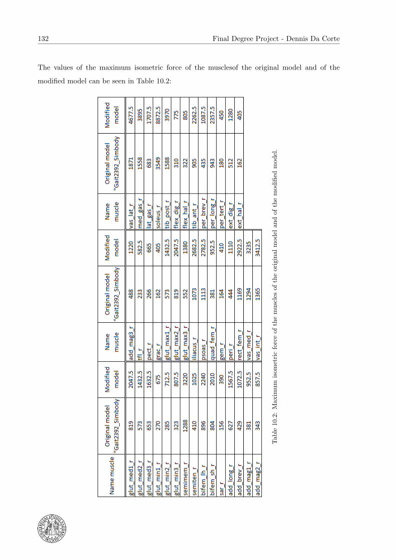
132 Final Degree Project - Dennis Da Corte
The values of the maximum isometric force of the musclesof the original model and of the
modified model can be seen in Table 10.2:
Tab
le10
.2:
Max
imu
mis
omet
ric
forc
eof
the
mu
scle
sof
the
ori
gin
al
mod
elan
dof
the
mod
ified
mod
el.
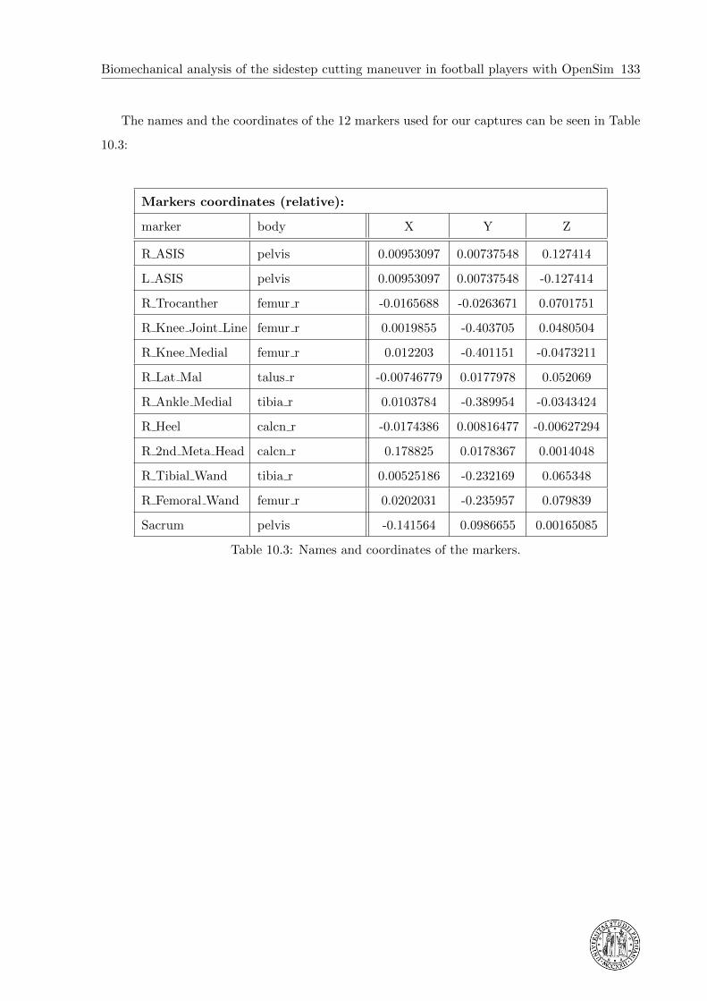
Biomechanical analysis of the sidestep cutting maneuver in football players with OpenSim 133
The names and the coordinates of the 12 markers used for our captures can be seen in Table
10.3:
Markers coordinates (relative):
marker body X Y Z
R ASIS pelvis 0.00953097 0.00737548 0.127414
L ASIS pelvis 0.00953097 0.00737548 -0.127414
R Trocanther femur r -0.0165688 -0.0263671 0.0701751
R Knee Joint Line femur r 0.0019855 -0.403705 0.0480504
R Knee Medial femur r 0.012203 -0.401151 -0.0473211
R Lat Mal talus r -0.00746779 0.0177978 0.052069
R Ankle Medial tibia r 0.0103784 -0.389954 -0.0343424
R Heel calcn r -0.0174386 0.00816477 -0.00627294
R 2nd Meta Head calcn r 0.178825 0.0178367 0.0014048
R Tibial Wand tibia r 0.00525186 -0.232169 0.065348
R Femoral Wand femur r 0.0202031 -0.235957 0.079839
Sacrum pelvis -0.141564 0.0986655 0.00165085
Table 10.3: Names and coordinates of the markers.
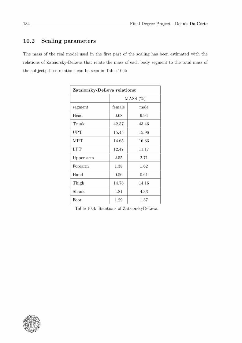
134 Final Degree Project - Dennis Da Corte
10.2 Scaling parameters
The mass of the real model used in the first part of the scaling has been estimated with the
relations of Zatsiorsky-DeLeva that relate the mass of each body segment to the total mass of
the subject; these relations can be seen in Table 10.4:
Zatsiorsky-DeLeva relations:
MASS (%)
segment female male
Head 6.68 6.94
Trunk 42.57 43.46
UPT 15.45 15.96
MPT 14.65 16.33
LPT 12.47 11.17
Upper arm 2.55 2.71
Forearm 1.38 1.62
Hand 0.56 0.61
Thigh 14.78 14.16
Shank 4.81 4.33
Foot 1.29 1.37
Table 10.4: Relations of ZatsiorskyDeLeva.

Biomechanical analysis of the sidestep cutting maneuver in football players with OpenSim 135
The set of measurement defined to run the first step of the scaling can be seen in Figure 10.1:
Figure 10.1: Set of measurement defined for the scaling.
The definition of the scale factors used to scale the model can be seen in the central column of
Figure 10.2, in the column at the right an example of the particular values of the scale factors
of one of the subjects:
Figure 10.2: Scale factors used for the Scaling.

136 Final Degree Project - Dennis Da Corte
The set of weights used for the second step of the Scaling can be seen in Figure 10.3. In the
first part the weights of the markers, on the second part the weights on the coordinates with
the desired values.
Figure 10.3: Weights used for the Scaling.

Biomechanical analysis of the sidestep cutting maneuver in football players with OpenSim 137
10.3 Inverse Kinematics parameters
The set of weights used for the Inverse Kinematics analysis can be seen in Figure 10.4. In the
first part the weights of the markers, in the second part the weights on the coordinates with the
desired values.
Figure 10.4: Weights used for the Inverse Kinematics analysis.
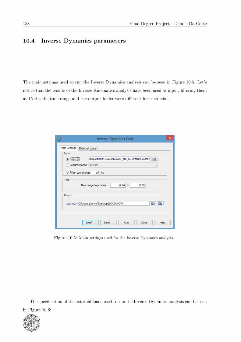
138 Final Degree Project - Dennis Da Corte
10.4 Inverse Dynamics parameters
The main settings used to run the Inverse Dynamics analysis can be seen in Figure 10.5. Let’s
notice that the results of the Inverse Kinematics analysis have been used as input, filtering them
at 15 Hz; the time range and the output folder were different for each trial.
Figure 10.5: Main settings used for the Inverse Dynamics analysis.
The specification of the external loads used to run the Inverse Dynamics analysis can be seen
in Figure 10.6:

Biomechanical analysis of the sidestep cutting maneuver in football players with OpenSim 139
Figure 10.6: Specification of the external loads used in the Inverse Dynamics analysis.

140 Final Degree Project - Dennis Da Corte
10.5 Static Optimization parameters
The main settings used to run the Static Optimization can be seen in Figure 10.7. In particular
as input we used the results of the Inverse Kinematics analysis with a cutting-off frequency of 15
Hz. In the “Objective Function” section we set the coefficient “p” equal to 2 and we unselected
the “Use muscle force-length-velocity relation”.
Figure 10.7: Main settings of the Static Optimization.

Biomechanical analysis of the sidestep cutting maneuver in football players with OpenSim 141
In the section “Actuators and External Loads” that we can see in Figure 10.8, we set the speifi-
cation of the external loads as we did for the Inverse Dynamics and we selected a file containing
a set of Residual Actuators useful to solve the inconsistency due to the missing parts of the body.
Figure 10.8: Settings of the Actuators and External Loads of the Static Optimization.
The Residual Actuators file contains the definition of 3 forces actuators (x, y and z direction)
and 3 torques actuators (x, y and z direction) and these are applied to the pelvis body.

142 Final Degree Project - Dennis Da Corte

Biomechanical analysis of the sidestep cutting maneuver in football players with OpenSim 143
Bibliography
[1] BODYSMART. Anatomi og fysiologi - et overblik. http://bodysmart.dk/hoften-pelvis.
[Online; accessed 26-January-2014].
[2] WIKIPEDIA COMMONS. Anterior cruciate ligament. http://en.wikipedia.org/wiki/
Anterior_cruciate_ligament. [Online; accessed 26-January-2014].
[3] WIKIPEDIA COMMONS. Pennation angle of fibers in pennate muscle. http://commons.
wikimedia.org/wiki/File:Pennation_angle_of_fibers_in_pennate_muscle.png.
[Online; accessed 26-January-2014].
[4] KRISTIANSLUND E. and KROSSHAUG T. Comparison of drop jumps and sport-specific
sidestep cutting: Implications for anterior cruciate ligament injury risk screening. 41(3):684-
8. Am J Sports Med., 2013.
[5] DE MORAT G., WEINHOLD P., BLACKBURN T., CHUDIK S., and GARRETT W.
Aggressive quadriceps loading can induce noncontact anterior cruciate ligament injury.
32(2):477-83. Am J Sports Med, 2004.
[6] KAMEN G., ROBERTSON D.G.E., and HAMILL J. Electromyographic Kinesiology. 2004.
[7] MYER G.D., FORD K.R., and HEWETT T.E. New method to identify athletes at high risk
of acl injury using clinic-based measurements and freeware computer analysis. 45(4):238-44.
Brit J Sport Med., 2010.
[8] LOEB G.E. and GHEZ C. The motor unit and muscle action. http://www.ib.cnea.gov.
ar. [Online; accessed 26-January-2014].
[9] KOGA H., NAKAMAE A., and SHIMA Y. Mechanisms of noncontact anterior cruciate
ligament injuries. 43(4): 396408. Am. J Sports Med., 2010.

144 Final Degree Project - Dennis Da Corte
[10] MATSUMOTO H. Mechanism of the pivot shift. 72(5):816-21. J Bone Joint Surg Br,
1990.
[11] WANG H. and ZHENG N. Knee rotation and loading during spin and step turn. 31(10):742-
6. Int J Sports Med., 2010.
[12] HICKS J. Getting started with rra. http://simtk-confluence.stanford.edu:8080/
pages/viewpage.action?pageId=3376194. [Online; accessed 27-January-2014].
[13] SPEER K., SPRITZER C.E., BASSETT F.H., FEAGIN J.A., and GARRETT W.E. Os-
seous injury associated with acute tears of the anterior cruciate ligament. 20(4):382-9. Am
J Sports Med., 1992.
[14] CARDINALE M. and LIM J. The acute effects of two different whole body vibration
frequencies on vertical jump performance. Med. Sport, 2003.
[15] HOUSTON METHODIST ORTHOPEDICS & SPORTS MEDECINE. A patient’s guide
to meniscal surgery. http://www.methodistorthopedics.com/bodyortho.cfm?id=41856.
[Online; accessed 26-January-2014].
[16] TOOLOOP HUMAN ANATOMY PICTURE. Back to post: Patella sesamoid bone.
http://www.tooloop.com/patella-sesamoid-bone/patella-sesamoid-bone. [Online;
accessed 26-January-2014].
[17] FAIRFAX COUNTRY PUBLIC SCHOOLS. Contraction of motor units.
http://staff.fcps.net/cverdecc/adv%20a&p/notes/muscle%20unit/contration%
20of%20motor/contraction_of_motor_units.htm. [Online; accessed 26-January-2014].
[18] SENIAM. Sensor placements. http://www.seniam.org/. [Online; accessed 26-January-
2014].
[19] MCLEAN S.G., HUANG X., SU A., and VAN DEN BOGERT A.J. Sagittal plane biome-
chanics cannot injure the acl during sidestep cutting. 19(8):828-38. Clin Biomech, 2004.
[20] SIMBIOS. Simtk. https://simtk.org/xml/index.xml. [Online; accessed 26-January-
2014].
[21] DELP S.L., ANDERSON F.C., ARNOLD A.S., LOAN P., HABIB A., JOHN C.T., GUEN-
DELMAN E., and THELEN D.G. Opensim: Open-source software to create and analyze
dynamic simulations of movement. 54(11):1940-50. IEE Trans Biomed Eng., 2007.

Biomechanical analysis of the sidestep cutting maneuver in football players with OpenSim 145
[22] HEWETT T.E., MYER G.D., and FORD K.R. Biomechanical measures of neuromuscular
control and valgus loading of the knee predict anterior cruciate ligament injury risk in
female athletes: a prospective study. 33(4):492-501. Am J Sports Med., 2005.

146 Final Degree Project - Dennis Da Corte

Biomechanical analysis of the sidestep cutting maneuver in football players with OpenSim 147
Chapter 11
Ringraziamenti
Questo lavoro di tesi e dedicato a voi Mamma e Papa, che mi avete sempre sostenuto durante
tutti questi anni, che mi avete dato l’ opportunita di studiare e di poter crescere professionalmente
nonche come persona, pur sapendo che molto probabilmente cio mi avrebbe portato lontano da
casa. Lontano da casa e dove ho trascorso gli ultimi 6 mesi della mia vita, tra un sacco di cose
nuove e stimolanti, ma anche senza la sicurezza di avere accanto qualcuno su cui poter contare
veramente, qualsiasi cosa potesse accadere. Vi ringrazio per avermi dato l’ opportunita di vivere
questa esperienza, pur sapendo quanto amara possa esser stata per voi; ne sono ritornato con un
importante bagaglio di vita vissuta e di esperienze che mai avrei potuto acquisire senza partire.
Finalmente siamo giunti insieme a questo importante traguardo della Laurea Magistrale e l’
unica cosa che posso dirvi e GRAZIE.
Vi voglio bene.
Dennis.


