113
Doctoral Thesis Department of Physics Lund Institute of Technology November 2002 BIOMEDICAL AND ATMOSPHERIC APPLICATIONS OF OPTICAL SPECTROSCOPY IN SCATTERING MEDIA Johannes Swartling

Doctoral Thesis
Department of Physics
Lund Institute of Technology
November 2002
BIOMEDICAL AND ATMOSPHERICAPPLICATIONS OF OPTICAL
SPECTROSCOPY IN SCATTERING MEDIA
Johannes Swartling

Copyright © 2002 Johannes Swartling
Printed at KFS AB, Lund, Sweden
November 2002
Lund Report on Atomic Physcs, LRAP-290
ISSN 0281-2162
LUTD2(TFAF-1050)1-113(2002)
ISBN 91-628-5486-0

Till Anette

5
Contents
Abstract 7List of papers 81. Introduction 112. Formulation of the problems 133. The forward problem – light propagation models 15
3.1 Electromagnetic wave theory 153.1.1 Models for single scattering based on
electromagnetic wave theory 163.1.2 Models for multiple scattering based on
electromagnetic wave theory 183.2 Transport theory of radiative transfer 20
3.2.1 Radiometric quantities 203.2.2 Transport properties 223.2.3 Scattering phase function 233.2.4 Reciprocity 243.2.5 Solving the transport equation 283.2.6 Polynomial approximations 293.2.7 Discretization methods; Adding-Doubling method;
Discrete ordinates 293.2.8 Expansion methods; The diffusion approximation;
The PN-approximation 343.2.9 Probabilistic methods; Photon migration; Path integrals 393.2.10 The Monte Carlo method 403.2.11 Variations on Monte Carlo simulations 443.2.12 Time-resolved and frequency-resolved calculations 473.2.13 Fluorescence and inelastic scattering 473.2.14 Photon hitting density and
photon measurement density functions 483.3 Discussion – solving the forward problem 50
3.3.1 Relationship between wave theory and transport theory 514. The inverse problem 53
4.1 Two-parameter methods 554.1.1 Spatially resolved diffuse reflectance 564.1.2 Time-resolved diffuse measurements 58
4.2 Three-parameter techniques; The integrating sphere method 594.3 Layered media and simple embedded inhomogeneities 644.4 Polynomial regression 64

6
4.5 Optical tomography 675. Practical aspects and applications 71
5.1 Tissue optical properties 715.1.1 Scattering properties of tissues 715.1.2 Absorption properties of tissues - chromophores 735.1.3 Water 745.1.4 Hemoglobin and myoglobin 745.1.5 Lipids 765.1.6 Melanin 775.1.7 Mitochondrial chromophores – cytochromes 785.1.8 Discussion – absorption properties of tissue 795.1.9 Optical properties of blood 80
5.2 Tissue phantoms 835.2.1 Water-based phantoms 835.2.2 Resin phantoms 845.2.3 Refractive index 85
5.3 Instrumentation 855.3.1 Cw measurement instruments 865.3.2 Frequency-resolved instruments 875.3.3 Time-resolved instruments 875.3.4 Optical tomography instruments 90
5.4 Optical mammography – a diagnostic application 915.5 Atmospheric optics – remote sensing of trace gases 92
Acknowledgements 95Summary of papers 96References 99

7
Abstract
Spectroscopic analysis of scattering media is difficult because the effective pathlength of the light is non-trivial to predict when photons are scattered many times.The main area of research for such conditions is biological tissues, which scatterlight because of variations of the refractive index on the cellular level. In order toanalyze tissues to diagnose diseases, or predict doses during, for example, lasertreatment, it is necessary to be able to model light propagation in the tissue, as wellas quantify the scattering and absorption properties. Problems of this type occur inmany other areas as well, for example in material science, and atmospheric andocean-water optics.
This thesis deals with light propagation models in scattering media, primarily basedon radiative transport theory. Special attention has been directed to the MonteCarlo model to solve the Boltzmann radiative transport equation, and to developfaster and more efficient computer methods. A Monte Carlo model was applied tosolve a spectroscopic problem in monitoring the emission of gases in smokeplumes. An important theme in the thesis deals with measurement of the opticalproperties, with emphasis on biomedical applications. Several differentmeasurement techniques based on a wide range of instruments have beendeveloped or improved upon, and the strengths and weaknesses of these methodshave been evaluated.
The measurement techniques have been applied to analyze the scattering andabsorption properties of some biological tissues. Much devotion has been directedto optical characterization of blood, which is an important tissue from a health-careperspective. At present, the complex scattering properties of blood preventsdetailed optical analysis of whole blood. The work presented here is also aimed atacquiring a better understanding of the fundamental scattering processes at acellular level.
8
List of papers
This thesis is based on the following papers:
Paper I. J. Swartling, A. Pifferi, A. M. K. Enejder, and S. Andersson-Engels, “Accelerated Monte Carlo model to simulate fluorescencespectra from layered tissues,” Journal of the Optical Society ofAmerica A, in press (2002).
Paper II. J. Swartling, J. S. Dam, and S. Andersson-Engels, “Comparison ofspatially and temporally resolved diffuse reflectance measurementsystems for determination of biomedical optical properties,”submitted to Applied Optics (2002).
Paper III. J. Swartling, A. Pifferi, E. Giambattistelli, E. Chikoidze, A. Torri-celli, P. Taroni, M. Andersson, A. Nilsson, and S. Andersson-Engels, “Measurements of absorption and scattering propertiesusing time-resolved diffuse spectroscopy – Instrumentcharacterization and impact of heterogeneity in breast tissue,”manuscript (2002).
Paper IV. J. Swartling, S. Pålsson, P. Platonov, S. B. Olsson, and S. Anders-son-Engels, “Changes in tissue optical properties due to radio-frequency ablation of myocardium,” submitted to Medical &Biological Engineering & Computing (2002).
Paper V. A. M. K. Enejder, J. Swartling, P. Aruna, and S. Andersson-Engels, “Influence of cell shape and aggregate formation on theoptical properties of flowing whole blood,” Applied Optics,returned after minor revisions (2002).
Paper VI. J. Swartling, A. M. K. Enejder, P. Aruna, and S. Andersson-Engels, “Polarization-dependent scattering properties of flowingwhole blood,” manuscript for Applied Optics (2002).
Paper VII. P. Weibring, J. Swartling, H. Edner, S. Svanberg, T. Caltabiano,D. Condarelli, G. Cecchi, and L. Pantani, “Optical monitoring ofvolanic sulphur dioxide emissions – Comparison between fourdifferent remote-sensing spectroscopic techniques,” Optics andLasers in Engineering 37, 267-284 (2002).

9
Additional material has been presented in:
1. S. Andersson-Engels, A. M. K. Enejder, J. Swartling, and A. Pifferi,"Accelerated Monte Carlo models to simulate fluorescence of layeredtissue," Photon Migration, Diffuse Spectroscopy, and Optical CoherenceTomography: Imaging and Functional Assessment, S. Andersson-Engels,J.G. Fujimoto, Eds. Proceedings of SPIE Vol. 4160, 14-15 (2000).
2. J. Swartling, P. Aruna, A. M. K. Enejder, and S. Andersson-Engels, "Opticalproperties of flowing bovine blood in vitro," Optical Techniques andInstrumentation for the Measurement of Blood Composition, Structure andDynamics In vitro and In vivo. CLEO/Europe 2000, Conference Digest p.354 (2000).
3. J. Swartling, C. af Klinteberg, J. S. Dam, and S. Andersson-Engels,"Comparison of three systems for determination of optical properties oftissue at 785 nm," European Conferences on Biomedical Optics (2001).
4. J. Swartling and S. Andersson-Engels, "Optical mammography - a newmethod for breast cancer detection using ultra-short laser pulses," DOPS-NYT 4, 19-21 (2001).
5. J. Swartling, S. Andersson-Engels, A. M. K. Enejder, and A. Pifferi,"Accelerated reverse-path Monte Carlo model to simulate fluorescence inlayered tissue," in OSA Biomedical Topical Meetings, OSA TechnicalDigest, 615-617 (2002).
6. J. Swartling, S. Pålsson, and S. Andersson-Engels, "Analysis of the spectralshape of the optical properties of heart tissue in connection with myocardialRF ablation therapy in the visible and NIR region," in OSA BiomedicalTopical Meetings, OSA Technical Digest, 607-609 (2002).
7. M. Ozolinsh, I. Lacis, R. Paeglis, A. Sternberg, S. Svanberg, S. Andersson-Engels, and J. Swartling, "Electrooptic PLZT ceramics devices for visionscience applications," Ferroelectrics 273, 131-136 (2002).
8. M. Soto Thompson, J. Swartling, S. Andersson-Engels, S. Pålsson, X. Zhao,“Dosimetry and fluence rate calculations for fiber-guided interstitialphotodynamic therapy: tissue phantom measurements and theoreticalmodeling,” BiOS 2003, San Jose (Accepted).

10
11
1. Introduction
The concept of spectroscopic analysis of materials is of profound importance inscience and technology. In traditional spectroscopy, the presence of a substancecan be detected and quantified by means of its spectral signature – wavelengthbands in which light is absorbed (or emitted), defined by the electronic energylevels of the atoms and molecules that constitute the substance. Measurements ofthis kind are performed routinely in thousands every day, to the benefit of themedical services, to industry and as a tool in basic research to promote theadvancement of our understanding of nature.
The conventional spectroscopic measurement requires that the material is opticallyclear. A simple definition of a clear material is that the refractive index is constanton spatial scales ranging from microscopic, in the order of the wavelength of thelight, up to macroscopic. Any spatial variation in the refractive index within thisrange will scatter light in a beam into new directions. To obtain quantitativeinformation from spectroscopy, it is necessary to know the path-length of the lightbeam through the medium. If the scattering of light is severe, the path-length nolonger represents the shortest distance from the light source to the spectrometerthrough the medium, but a longer one, which is not trivial to predict. Light scattersto some extent in all media, but in many cases the effect is so small that it may beneglected. In an intermediate regime, the scattering may be significant, but stillsmall enough so that the assumption of a clear medium can be used with suitablecorrections. One of the main objectives of this thesis is to deal with the predictionof the light path-length through media where the scattering is so strong that suchcorrections are no longer valid.
There is no clear delineation where the weakly scattering regime stops and thestrongly scattering regime starts – it depends on the problem. Often, one talksabout multiple scattering. If light is regarded as photons, multiple scattering occurswhen there is a large probability that any given photon in a beam will scatter morethan once. Then it is evident that a strongly scattering medium is characterized bytwo things: the probability of scattering, and the dimensions of the medium. Forexample, a piece of paper has a very high probability of scattering, and scatterslight strongly even though its physical dimensions are small. On the other hand, theprobability of scattering in the atmosphere is comparably low, but taken overseveral kilometers, the scattering of a light beam may still be significant. Anotherobjective of this thesis is to show that the same models and principles may beapplied to very small geometries, such as sheets of paper, and very large ones, suchas atmospheric measurements.
Examples of strongly scattering media that are interesting from a spectroscopicpoint of view include the already mentioned paper and atmosphere, ocean water, a

12
large number of solid materials around us, and most biological tissues. Since theinvention of the laser in the 1960s, and its rapid adoption by the medicalcommunity, tissue optics has been the major field of research where stronglyscattering media have been studied. In the study of tissue optics, the third mainobjective of this thesis becomes clear: the scattering of a material is not only anuisance in spectroscopic measurements. By analyzing the scattering properties,important information of the material may be obtained. Thus, the scattering itselfbecomes an object of analysis rather than just a parameter to be controlled.
Although research in tissue optics took off during the 1970s, it is of historicalinterest to note that much of the fundamental theory was developed earlier, in otherbranches of physics. As will be described in this thesis, light scattering is usuallymodeled from a starting point of either of two theories: wave theory (Maxwell’sequations) or transport theory. Much of the theory of scattering from singleparticles using wave theory was developed in the early years of the 20th century.Transport theory originates from the late 19th century, but the development wasaccelerated with the need to model neutron transport in nuclear reactors. Much ofthe relevant literature and computer code used for light propagation was inheritedby research in neutron transport.
In medical applications of light and lasers, the whole range of important issues oflight propagation in scattering media is demonstrated. A fundamentalcategorization is the forward problem and the inverse problem. The forwardproblem is, given that the optical properties of the medium are known, to predicthow light will propagate through the medium. The practical importance of this inmedical applications is mainly in therapy, for example to calculate the dose in alaser treatment. The inverse problem is, given that light that has penetrated thetissue is measured, to deduce what the optical properties inside the medium are.The practical importance here is mainly in diagnostics, since both the absorptionproperties – the traditional spectroscopic signal – and the scattering propertiescarry information on the state of the tissue. The other important aspect of theinverse problem is to provide input data for calculations of the forward problem.However, as will be seen, it is not possible to solve the inverse problem withoutfirst solving the forward problem.
This thesis concerns models of light propagation in scattering media, with theemphasis on transport theory. Specifically, the Monte Carlo method was usedextensively in Papers I and VII. Measurement of the optical properties is anothermajor part of the thesis, and Papers II – VI are devoted to this problem. Most workhas been done within the framework of potential practical applications, primarily inmedicine (Papers I – VI) but also in environmental monitoring (Paper VII).

13
2. Formulation of the problems
From a very general perspective, consider Fig. 2.1. A turbid medium, delineated bya boundary, is illuminated from the outside, or by light sources from inside, withlight Xin(r,s,t). The denotation X represents some suitable radiometric quantity, rrepresents the spatial coordinates, s is a direction and t time. For simplicity the lightis assumed monochromatic. The medium has optical properties denoted p(r), forthe moment disregarding their physical origin. It is usually assumed that p(r) isquasi-constant in time, i.e., any changes in the optical properties occur on a longertime scale than the propagation of light. Light that either propagates through themedium or has emerged is denoted Xprop(r,s,t).
The Forward Problem
The first task is to find a way to predict Xprop(r,s,t), given that we know p(r).Thus, we want to find the transfer function f:
f[Xin(r,s,t);p(r)] → Xprop(r,s,t) (2.1)
The Inverse Problem
The next task is to find a way to deduce p(r), given that we have measuredXprop(r,s,t), or some part of it. This means finding the inverse to the above:
f-1[Xin(r,s,t);Xprop(r,s,t)] → p(r) (2.2)
These problems comprise the fundamental questions posed in this thesis. In orderto solve the forward and the inverse problem for a turbid medium, a number ofphysical theories, assumptions and approximations are needed. In the next chapter,the forward problem will be discussed, followed by the inverse problem inChapter 4. To conclude, some practical aspects concerning tissue optics,instrumentation issues, and applications are discussed in Chapter 5.

14
FigmeXinXpr
p(r)X (r,s,t)in
X (r,s,t)prop
. 2.1 The geometry of light propagation in a turbid medium, in general terms. Thedium is delineated by a boundary, and it is illuminated by light represented by(r,s,t). The light that propagates through the medium, or has emerged, is denotedop(r,s,t). The optical properties are denoted p(r).

15
3. The forward problem – light propagation models
The definition of the optical properties p(r) in Fig. 2.1 depends on the physicaltheory one chooses to describe the light propagation. As mentioned in theintroduction, either of two physical theories of light is considered: wave theory ortransport theory. Wave theory, or electromagnetic wave theory, relies on solutionsof the Maxwell equations. In this context, the optical properties are defined by thecomplex dielectric constant, ε(r). The variation in Re{ε(r)} describes thescattering, while Im{ε(r)} represents the absorption properties. Only in specialcases is it possible to solve the wave equation for large macroscopic problems, aswill be discussed later. In most problems, especially those related to tissue optics, itis intractable both to solve the wave equation and to cope with the vast complexityof the variation of ε(r) on a microscopic level. To deal with such problems, thetransport theory of radiative transfer is better suited. In transport theory, light isheuristically regarded as energy propagating according to the rules defined by thetransport equation, a conceptually simple equation of conservation. The opticalproperties p(r) are defined by means of a scattering coefficient, an absorptioncoefficient and a scattering phase function which relates to the probability ofscattering in different directions.
In the next sections, some relevant parts of electromagnetic wave theory, transporttheory and their relation will be described. Because of the vast number ofpublications on the basic theory of these subjects already available, the followingtreatment will focus on the use of the models rather than full theoreticalderivations.
3.1 Electromagnetic wave theoryMaxwell’s equations form the starting point of the description of light propagationas electromagnetic waves propagating through a dielectric medium. The fields areclassically described by:
t∂∂
−=×∇BE (3.1)
FDH +∂∂
=×∇t
(3.2)
ρ=⋅∇ D (3.3)
0=⋅∇ B (3.4)

16
where E [Vm-1] and H [Am-1] are electric and magnetic field vectors, B [Vsm-2] isthe magnetic flux density vector, D [Asm-2] is the electric displacement vector, F[Am-2] is the current density vector (the conventional notation J is in this thesisreserved for the radiometric quantity radiant flux density, see Eq. (3.8) – (3.11)),and ρ [Asm-3] is the volume charge density. The electric and magnetic fields can berelated to the displacement field and flux density fields by constitutive relations,depending on the properties of the medium. In a non-dispersive isotropic medium,which we are interested in here, the relations are D = εE and B = µH, where ε[AsV-1m-1] is the permittivity and µ [VsA-1m-1] is the permeability. The currentdensity and the electric field are also coupled by F = σE, where σ [AV-1m-1] is theconductivity.
The Maxwell equations can be solved directly using numerical methods, which willbe discussed below. The computations for large problems are daunting, however,and clever use of expansion methods and approximations can greatly reduce thecalculations needed for some problems. Typically, it is assumed that the medium isnonconductive, and one can then derive the vector wave equations (or Helmholtzequations)1:
022 =+∇ EE k (3.5)
022 =+∇ HH k (3.6)
where k = 2π/λ is the wavenumber (λ is the wavelength).
Often, one is interested in prediction of the scattering from single particles, bothbecause many scattering media in fact consist of ensembles of particles, and alsobecause sometimes it is possible to assume that a scattering medium may beapproximated by scattering particles. Scattering from particles can be described interms of diffraction2,3 or approximations such as those presented by Rayleigh-Gans-Debye2-4, but more general approaches are given by Mie theory and T-matrixtheory. Mie theory deals with spherical particles, while T-matrix theory isapplicable to particles of arbitrary shape, although in practice only particles ofspheroidal symmetry are useful. The general idea in Mie and T-matrix theory is toexpand the fields in vector spherical functions.
3.1.1 Models for single scattering based on electromagnetic wave theoryMie theory (or Lorenz-Mie theory) provides a quick and relatively simple way ofcalculating light scattering2,3. The relevant input parameters to a Mie calculationare the ratio of the refractive index inside the particle to that in the surroundingmedium, m = nparticle/nmedium, and the size parameter x = 2πa/λ, where a is the

17
radius of the particle. The result of a Mie calculation is a map of the scattered fieldfrom an incident plane wave. Usually, one is interested in the extinction crosssection Cext [m2], scattering cross section Csca [m2], and the absorption crosssection Cabs [m2] of the particle. These can be obtained through integration of thescattered field, and are related as Cext = Csca + Cabs. It is also convenient to definerelative extinction, scattering and absorption cross sections, Qext, Qsca and Qabs(dimensionless). The relative scattering cross section is defined as Qsca = Csca/πa2,and the others analogously. Another property of interest is the scattering anisotropyfactor, g = <cosθ>, where θ is the scattering angle. The anisotropy factor is ameasure of how close to isotropic the scattering is. For entirely isotropic scattering,such as Rayleigh scattering, g = 0. In this context it can also be noted that Mietheory collapses to the classical Rayleigh expression for scattering when x → 0 (cf.Eq. 5.6).
The applicability of Mie theory on a problem depends on several factors. Particlesthat are spherical by nature are of course prime candidates. Examples of this kindare liquid aerosols such as water droplets. Particles of irregular shape can also bemodeled successfully using Mie theory under certain conditions. Several studieshave shown that in an ensemble of randomly oriented particles of nonsphericalshape, the average scattering can often be represented by Mie theory of spheres ofequivalent size. However, this is not always the case, as some authors have pointedout5. Mie theory is also important for validation purposes. Instruments designed tomeasure the scattering of a medium can be tested on samples with microsphereswith known size and refractive index, to serve as a verification against theory. Thisis discussed in more detail in Sect. 5.2. Finally, Mie calculations are useful toprovide quick and approximate results when only order-of-magnitude numbers areneeded for media that consist of irregular scattering structures.
Mie calculation is not entirely trivial, and the computations are susceptible toround-off errors in the numerical routines. New Mie codes therefore have to betested thoroughly. For this reason, it is usually best to try to find an existing, well-tested program. In this thesis, all Mie calculations were performed using theprogram by Bohren and Huffman, BHMIE3. Mie programs are available on theInternet, also as interactive web scripts6.
T-matrix theory presents a more general method to calculate scattering fromparticles of other shapes than spherical5,7. In principle, any shape is possible, butdue to the fact that the field vector expansion is based on vector sphericalfunctions, spheroidal particles are best suited. The calculations are even moresensitive to round-off errors than Mie theory, especially as the size parameterincreases. For practical purposes, only particles of some spherical symmetry arepossible because of this. T-matrix calculations were performed to study thescattering from red blood cells in Paper V. A modified version of the code by

18
Barber and Hill was used8,9. Single-precision (16 digits) T-matrix computations arepossible for size parameters x < 25, but with extended precision (32 digits) sizeparameters up to around x = 65 are possible with good accuracy10.
3.1.2 Models for multiple scattering based on electromagnetic wave theoryEnsembles of particles are possible to model using Mie or T-matrix theory, as longas the distances between the particles are large. The total scattering coefficient canthen easily be calculated, because the individual particles are in the scattering far-field with respect to their neighbors. When the interparticle distances becomesmall, the particles start to influence each other in their near-field, and theassumption of single, independent scatterers breaks down. In some cases,aggregates of a small number of particles are possible to model using Mie or T-matrix theory using a superposition approach7,11, but for more complicatedgeometries more general methods are required. The perhaps most straightforwardmethod of solving a wave problem for an arbitrary geometry is by discretizingMaxwell’s equations, the spatial coordinates and time. This method is called FiniteDifference Time Domain (FDTD), and can in principle solve any problem.However, due to the computational requirements, FDTD is limited to rather smallproblems. As a rule of thumb, the spatial discretization must be λ/15 or smaller,which means about 106 points for a problem of size 5λ. For each time step, oneoperation is required for every point in space. More information on FDTD can befound in Refs. 12 and 13. Calculation of light scattering from single biological cellsusing FDTD has been demonstrated14-16.
An alternative approach to FDTD is to use the Finite Element Method (FEM) tosolve Maxwell’s equations. In general, FEM is best suited to solve partialdifferential equations on closed domains, i.e., boundary value problems. FEMrequires the medium to be represented by a mesh, and one of the principaladvantages of the method is the versatility of the mesh design and flexibility ofrepresenting complicated shapes and variations in dielectric constant. Anotheradvantage of FEM is that the matrices are typically sparse, so that the numericalmachinery that pertains to sparse matrix computation can be utilized. A drawbackof the method is that special care has to be taken when modeling unboundeddomains, to terminate the mesh using the proper boundary conditions. Severalcommercial and free FEM codes are available, ranging from very simple 2Drepresentations to advanced packages. Examples of free codes are EMAP17 andStudent’s QuickField18, while commercial software packages include FEMLAB (aMatlab toolbox)19 and EMFLex20.
19
A slightly less direct approach is presented by the Method of Moments (MoM). Inthis method, the problem is reduced to smaller domains, where the Maxwellequations are formulated as integral equations21. An example of a free MoM codeis PCB-MoM22.
The methods mentioned so far suffer from being restricted by the computationalresources required for problems larger than a few wavelengths. Larger problems,up to a few hundred wavelengths, can be solved using the Fast Multipole Method(FMM)23. FMM utilizes an efficient method for numerical convolution of theGreen’s function for the vector wave equation, which leads to a reduction of thenumerical complexity. The method does not inherently involve anyapproximations, but by utilizing problem-specific properties the computation canbe made even more efficient. One such assumption may be that the variation inrefractive index in the medium is small. This condition is fulfilled in human blood,which renders FMM a possible candidate for modeling the complex scatteringproperties of blood (see also Sect. 5.1.9; Optical properties of blood).
To solve even larger problems, approximation methods can be used. Theapproximation methods are sometimes denoted asymptotic methods, which in turncan be categorized into four classes: approximations of partial differentialequations and integrals, geometrical optics, physical optics, and other methods. Asan example from the first area, the vector wave equation, which is elliptic, may beapproximated by a paraxial equation, which renders the parabolic equationmethod24. This method is suitable for large problems with a clear, preferreddirection of propagation. A closely related approach is the Bremmer seriesmethod25.
Geometrical optics is valid when the curvature of the object is large compared withthe wavelength, i.e., typically for large objects. The ray trajectories are given by thefamous Fermat’s principle, stating that the path of a ray is always such that theoptical path length is minimized. Geometrical optics problems can be solved usingray tracing software. Physical optics depends on integral representations of the farfield, for scatterers that are perfectly conducting. The requirement of large objectsholds for physical optics as well. The two methods can be combined with othermethods, such as MoM, if smaller objects are involved in the problem. The lastcategory, other methods, includes simple optical models such as ray tracingwithout a phase front, and Fraunhofer and Fresnel diffraction.
The results from the wave equation can also be used as a starting point for arigorous, analytical derivation of statistical quantities relevant for multiplescattering problems. This leads to differential or integral equations that, inprinciple, include all wave effects. However, the solutions are complicated and inpractice various approximations are employed. Examples of methods include

20
Twersky’s theory, the diagram method, and the Dyson and Bethe-Salpeterequations. An overview of analytical theory is given by Ishimaru26. Twersky’stheory has been applied on the problem of light scattering in human blood27,28 (cf.Sect. 5.1.9; Optical properties of blood). However, the result of Twersky’s theoryis equations with parametric dependence, where the parameters cannot be easilydeduced from considerations of the fundamental geometrical and dielectricproperties of the medium. In terms of practicality, the theory is therefore moresimilar to transport theory, which is the topic of next section.
3.2 Transport theory of radiative transferThe radiative transport equation (RTE) (or Boltzmann equation) can be stated as
),,q()(d)',p(),,(),,()(),,(
),,(1
4
ttLtLtLt
tLc
ssa srssssrsrsrs
sr
+ωµ+µ+µ−∇⋅−=
=∂
∂
∫π
(3.7)
The RTE is an equation of conservation, describing the change in radiance L in thedirection s inside a small volume element dV. Thus, the first term on the right handside describes the losses over the boundary of dV, the next term the losses due toabsorption and scattering, the third term the gains due to scattering from otherdirections into s, and the last term gains due to any source q inside dV29,30. Definingthe remaining designations introduced, starting from the left, we have the lightspeed in the medium c [m/s], the absorption coefficient µa [m-1], the scatteringcoefficient µs [m-1], and the scattering phase function p(s,s') [-]. The scatteringphase function gives the probability of scattering from direction s' into direction s.In the integral, dω(s) denotes an infinitesimal solid angle in the direction s.
Classical, and still essential, references on transport theory include the works byChandrasekhar31, Case and Zweifel29, and Ishimaru26. A recent treatment, orientedtoward tissue optics, is given in Ref. 30.
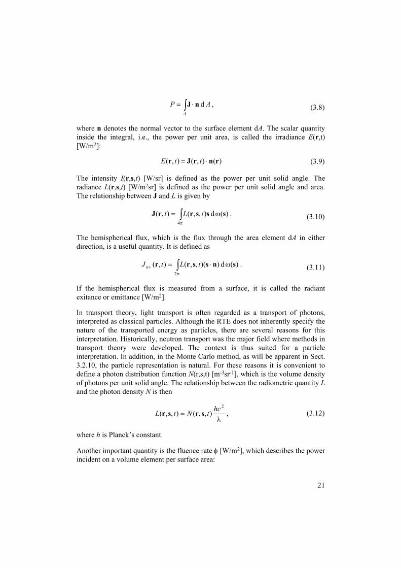
3.2.1 Radiometric quantitiesBefore discussing the RTE further, it is useful to define some radiometricquantities and their relationships. The radiant flux density J [W/m2] is defined asthe power P transferred through a surface area A:
21
APA
d ∫ ⋅= nJ , (3.8)
where n denotes the normal vector to the surface element dA. The scalar quantityinside the integral, i.e., the power per unit area, is called the irradiance E(r,t)[W/m2]:
)(),(),( rnrJr ⋅= ttE (3.9)
The intensity I(r,s,t) [W/sr] is defined as the power per unit solid angle. Theradiance L(r,s,t) [W/m2sr] is defined as the power per unit solid angle and area.The relationship between J and L is given by
)(d ),,(),(4
sssrrJ ω= ∫π
tLt . (3.10)
The hemispherical flux, which is the flux through the area element dA in eitherdirection, is a useful quantity. It is defined as
)(d ))(,,(),(2
snssrr ω⋅= ∫π
+ tLtJ n . (3.11)
If the hemispherical flux is measured from a surface, it is called the radiantexitance or emittance [W/m2].
In transport theory, light transport is often regarded as a transport of photons,interpreted as classical particles. Although the RTE does not inherently specify thenature of the transported energy as particles, there are several reasons for thisinterpretation. Historically, neutron transport was the major field where methods intransport theory were developed. The context is thus suited for a particleinterpretation. In addition, in the Monte Carlo method, as will be apparent in Sect.3.2.10, the particle representation is natural. For these reasons it is convenient todefine a photon distribution function N(r,s,t) [m-3sr-1], which is the volume densityof photons per unit solid angle. The relationship between the radiometric quantity Land the photon density N is then
λ=
2
),,(),,( hctNtL srsr , (3.12)
where h is Planck’s constant.
Another important quantity is the fluence rate φ [W/m2], which describes the powerincident on a volume element per surface area:

22
)(d),,(),(4
ssrr ω=φ ∫π
tLt . (3.13)
The fluence rate is useful since by knowing the absorption in the medium, theabsorbed energy W [J/m3] can be calculated as
ttW a d),()()( ∫ φµ= rrr . (3.14)
This equation is important, since it couples the deposited energy – dose – in amedium, to the radiometric quantity fluence rate.
3.2.2 Returniparameand scacoefficiscattericonside
E
E0
E = E exp(-µ d)0 t
µ t
xd
Fig. 3.1 Illustration of Beer-Lambert’s law.
Transport propertiesng to the discussion about the RTE, one identifies four medium-dependentters: the light speed c – determined by the refractive index, the absorptionttering coefficients µa and µs, and the scattering phase function p(s,s'). Theents µa and µs should be interpreted as the probability of absorption andng per unit path length, respectively. Their meaning is clear whenring the generalized Beer-Lambert law,
[ ]dEE sa )(exp0 µ+µ−= , (3.15)

which describes the attenuation of a collimated beam (plane wave) of initialirradiance E0 through a medium of thickness d (see Fig. 3.1). Within theframework of the particle interpretation, the reciprocal of µa + µs, 1/(µa + µs), isinterpreted as the mean free path length between photon interactions with themedium. The quantity µt ≡ µa + µs is called the total attenuation coefficient.
3.2.3 Scattering phase functionThe scattering phase function p(s,s') describes the angular probability of scatteringfrom direction s' to s. The phase function is sometimes written as p(cosθ) toemphasize the angular dependency, and although this is only possible when there isno absolute directional dependency, physically realistic phase functions virtuallyalways only exhibit relative angular dependency. It is usually assumed that thescattering probability is symmetric for the azimuthal angle ψ, although this is not astrict requirement. The phase function is normalized:
1)d(cos )p(cos1
1
=θθ∫−
. (3.16)
To exemplify the microscopic spherthe diameter incre
Fig. 3.2 ScIn the calc
attered field from spherical particle calculated with Mie theory.ulation, m = 1.5, and x = 2π. The anisotropy factor is g = 0.58.
23
importance of the phase function, consider the scattering from ae, as described by Mie theory (see Fig. 3.2). As a general rule, asases the scattering gets increasingly forward-favored. Lobes are
24
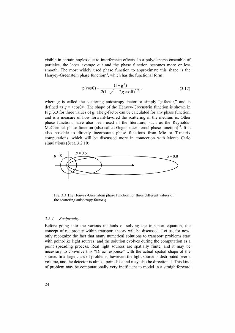
visible in certain angles due to interference effects. In a polydisperse ensemble ofparticles, the lobes average out and the phase function becomes more or lesssmooth. The most widely used phase function to approximate this shape is theHenyey-Greenstein phase function32, which has the functional form
2/32
2
)cos21(2)g1()p(cos
θ−+−
=θgg
, (3.17)
where g is called the scattering aniostropy factor or simply “g-factor,” and isdefined as g = <cosθ>. The shape of the Henyey-Greenstein function is shown inFig. 3.3 for three values of g. The g-factor can be calculated for any phase function,and is a measure of how forward-favored the scattering in the medium is. Otherphase functions have also been used in the literature, such as the Reynolds-McCormick phase function (also called Gegenbauer-kernel phase function)33. It isalso possible to directly incorporate phase functions from Mie or T-matrixcomputations, which will be discussed more in connection with Monte Carlosimulations (Sect. 3.2.10).
3.2.4Befoconconlywithpoinnecesourvoluof p
g = 0 g = 0.5g = 0.8
Fig. 3.3 The Henyey-Greenstein phase function for three different values ofthe scattering anisotropy factor g.
Reciprocityre going into the various methods of solving the transport equation, theept of reciprocity within transport theory will be discussed. Let us, for now, recognize the fact that many numerical solutions to transport problems start point-like light sources, and the solution evolves during the computation as at spreading process. Real light sources are spatially finite, and it may bessary to convolve this “Dirac response” with the actual spatial shape of thece. In a large class of problems, however, the light source is distributed over ame, and the detector is almost point-like and may also be directional. This kindroblem may be computationally very inefficient to model in a straightforward
25
way. The reciprocal situation could then be a much more efficient model, providedthat one can show that the two situations are equivalent.
Reciprocity was used in both Papers I and VII, and therefore a more detailedderivation of the reciprocity theorem within transport theory will be presented here.The derivation essentially follows that in Ref. 29. Consider the RTE, Eq. (3.7). Thetime-dependent RTE can always formally be reduced to a time-independentequation through a Laplace transform29. Therefore, we only have to derive thereciprocity theorem for the time-independent RTE:
),()(d)',p()',(),()(),(4
srssssrsrsrs QLLL ssa +ωµ=µ+µ+∇⋅ ∫π
. (3.18)
Let L1(r,s) be the unique solution to Eq. (3.18) for a given source Q1(r,s) andincident distribution Linc,1(ρ,s) on the surface S of the volume V:
),,()(d)',p()',(),()(),( 14
111 srssssrsrsrs QLLL ssa +ωµ=µ+µ+∇⋅ ∫π
0 ),,(),( 1,1 <⋅ρ=ρ nsss incLL .(3.19)
A unique solution always exists if µa > 0. Let ),(~1 srL be the solution to an RTE
identical to (3), except that
),'p()',p( ssss −−→ , (3.20)
i.e.,
),,()(d),'p()',(~),(~)(),(~1
4111 srssssrsrsrs QLLL ssa +ω−−µ=µ+µ+∇⋅ ∫
π
0 ),,(),(~1,1 <⋅ρ=ρ nsss incLL .
(3.21)
Now, if the phase function p is invariant under time reversal, we have
)',p(),'p( ssss =−− , (3.22)
and it is clear that ),(),(~11 srsr LL = since they are both unique solutions to the
same equation with the same boundary conditions. Furthermore, we can define twosolutions L2(r,s) and ),(~
2 srL in a similar way. Since we are deriving an expressionfor reciprocity, the quantity we are interested in is ),(~
2 sr −L . This gives theequation
26
),,()(d),'p()',(~),(~)(),(~1
4222 srssssrsrsrs −+ω−µ=−µ+µ+−∇⋅− ∫
π
QLLL ssa
0 ),,(),(~2,2 >⋅ρ=−ρ nsss incLL .
(3.23)
Now, multiply Eq. (3.19) by ),(~2 sr −L , and integrate over V and s:
∫ ∫∫ ∫ ∫
∫ ∫∫ ∫
ππ π
ππ
ω−+ωω−µ
=ω−µ+µ+ω−∇⋅
VVs
Vsa
V
VLQVLL
VLLVLL
421
4 412
421
421
d)(d),(~),(d)(d)'(d)',p()',(),(~
d)(d),(~),()(d)(d),(~),(
ssrsrsssssrsr
ssrsrssrsrs
(3.24)
Similarly, multiply Eq. (3.23) by L1(r,s) and integrate over V and s, and subtractfrom Eq. (3.24). The divergence term can be simplified to a surface integral usingGauss’ theorem, and we obtain:
{ }
{ }∫ ∫ ∫
∫ ∫
∫ ∫
π π
π
π
ωω−−−µ
+ω−−−
=ω−⋅
Vs
V
S
dVLLLL
VLQLQ
SLL
4 42112
41221
421
)(d)'(d ),'p(),(~)',()',p()',(),(~
d)(d ),(),(),(~),(
d)(d),(~),()(2
sssssrsrsssrsr
ssrsrsrsr
ssrsrns
(3.25)
The last term vanishes because we can make the variable transformation 'ss ↔ .Since we had assumed that p(s,s') was invariant under time reversal, and thus that
),(),(~22 srsr LL = , we finally obtain
{ }∫ ∫
∫ ∫
π
π
ω−−−
=ω−⋅
V
S
VLQLQ
SLL
41221
421
dd ),(),(),(),(
dd),(),()(2
srsrsrsr
srsrns
(3.26)
Equation (3.26) expresses the reciprocity theorem on integral form.
Proceeding to derive the reciprocity theorem in the case usually encountered intissue optics, consider the geometry in Fig 3.4. It is clear that Q1 is an isotropicsource inside the volume V:
)(4
),( 11
1 rrsr −δπ
=P
Q . (3.27)

wheof tthe possoudef
whethe reflrefr
Fmdgsothr2
(b) Reverse
r1
r2
n
∆ωn1
n2
Q1r1
r2
n
∆ωn1
n2
Q2
Direction ofpropagation
OO
Direction ofpropagation
(a) Forward
ig. 3.4 Reciprocity used in tissue optics. The refractive indices outside and inside theedium are denoted n1 and n2, respectively. The normal vector at the surface is
enoted n. In (a), the forward case, we have an isotropic light source Q1 at r1 thatives rise to a flux over the boundary at r2. The radiance at r2 is integrated over thelid angle ∆ω, which may be determined by the condition for total reflection, or bye collection angle of a detector at r2. In (b), the reverse case, a surface source Q2 at gives rise to a fluence rate at r1. The source Q2 emits in the solid angle ∆ω.
27
re P1 is the power emitted by the source. For the reciprocal case, the definitionhe light source is less obvious. Apparently, we could define an incident light onboundary Linc,1(ρ,s) and let Q2 be zero. However, it turns out that it is alwayssible to replace an incident light distribution with an equivalent surfacerce29. This means that the left-hand side of Eq. (3.26) vanishes, and we canine a surface source Q2 as
ω∆
ω∆−δ−⋅ω∆=
insidenot is if 0
inside is if )()(),( 2
2
2
s
srrnssr FrP
Q (3.28)
re P2 is the emitted power, rF is a factor that accounts for Fresnel reflection atinterface, and the solid angle ∆ω is defined by the critical angle for total
ection at the boundary (or the collection angle of a detector at r2). In case theactive indices are equal, ∆ω = 2π. Hence, we get:
∫∫ω∆π
ω−⋅−ω∆
=ωπ
)(d ))(,()(d ),(4 21
2
412
1 snssrssr FrLPLP . (3.29)

28
The integral on the left-hand side is exactly the fluence rate at r1 due to the surfacesource Q2(r,s), while the integral on the right-hand side is exactly the radiant fluxdensity at the surface at r2 due to the isotropic source Q1(r,s). In practice, we areinterested in the case when these two quantities are equal, and we get
12 4PP
πω∆
= . (3.30)
Thus, to get the same result from two reciprocal computations, the powers of thetwo reciprocal sources should be scaled according to Eq. (3.30). A more detailedderivation of Eqs. (3.27) – (3.30) is given in Paper I.
As we have seen, the reciprocity theorem is valid under the assumption that thephase function is invariant under time-reversal,
)',p(),'p( ssss =−− . (3.31)
A natural question is whether there are any physically relevant phase functions thatdo not exhibit this kind of invariance. Starting with the Henyey-Greenstein phasefunction, Eq. (3.17), we see that there is no dependence on the direction s and thuswe are free to make the variable substitution in Eq. (3.31) without violating theequality. The same is true for any phase function computed from Mie theory,which is clear because of the symmetry of spherical particles. For any normalscattering conditions it seems that we can assume that the time-reversal invarianceof the phase function holds.
3.2.5 Solving the transport equationA range of different techniques to solve the RTE are available, each with itsadvantages and drawbacks. First, we note that no analytical solutions to the RTEare available in 3D, for any geometry other than such that can be represented in oneor two dimensions. Full solutions of the RTE are only possible using numericalmethods, e.g. by discretization of the equation. The most widely used discretizationmethod is the discrete ordinates method, which will be described in Sect. 3.2.7. Theother option is the use of Monte Carlo simulations, a method that has been widelyadopted by the tissue optics community.
Instead of attempting a full solution, various methods based on simplifications orapproximations are available. Sometimes, the dimensionality of the problem can bereduced. For a few, special, but important geometries, polynomial approximationshave been developed. Perhaps the most important approximation is the diffusion

29
approximation, which is based on the first terms in a spherical harmonicsexpansion.
In the next few sections, emphasis will be turned to the Monte Carlo simulationmethod, but most of the other important methods for solving the transport equationwill be reviewed or at least be given reference to. As before, the treatment focuseson the practical aspects of the methods rather than derivations, which can be foundin the references.
3.2.6 Polynomial approximationsPolynomial approximations have no physical meaning and are not solutions to theRTE per se, but they may be useful tools for quick calculations. The idea is to finda polynomial expression describing the optics of the medium using one parameter.A useful example is the total reflectance from a semi-infinite medium, illuminatedwith diffuse light. This has been found to follow34
sssR
17.11)139.01)(1(
+−−
= , (3.32)
where
agas
−−
=11
(3.33)
and a is the albedo, a = µs/(µa+µs). The error of prediction has been shown to beless than 0.003 for any combination of µs, µa and g. More on polynomialapproximations can be found in Ref. 34. Approximations for collimated incidentlight, also for index mismatch between the semi-infinite media, can be found inRef. 35.
3.2.7 Discretization methods; Adding-Doubling method; Discrete ordinatesAs already discussed in connection with the vector wave equations, the moststraightforward way of solving complex equations is by direct discretization andsubsequent numerical computations. A first step in discretization of the RTE is todiscretize the radiance in angular components, s1, s2, ...sN. The equation can then bewritten as
30
),(),p(),(),(),(1
ijijiii srsssrsrsrs QLwLLN
jjst +µ=µ+∇⋅ ∑
=
, (3.34)
where wj are weighting factors used in the quadrature. This general approach iscalled the discrete ordinates method or the N-flux method. The simplest way ofdealing with this equation is to include only one angular component, the forwarddirection. In this context the radiance is not a useful quantity since it is defined bymeans of solid angles. Instead, one must use the irradiance. The RTE is thenreduced to
)()( xEdx
xdEtµ−= , (3.35)
which has the solution
)exp()0()( txxExE µ−== (3.36)
recognized as Beer-Lambert’s law.
Increasing complexity slightly, we include two angular components, the forwardand the reverse directions. This is the 2-flux, or one-dimensional, transport theory.The one-dimensional transport equation is a set of coupled differential equations:
)()()()(1 xExE
dxxdE
a −++ σ+σ+µ−= (3.37)
)()()()(1 xExE
dxxdE
a +−− σ+σ+µ−=− . (3.38)
Here, E+(x) propagates in the positive x direction, and E-(x) in the negative. µa1 isthe one-dimensional absorption coefficient, and σ = µs1p(–x,x) = µs1p(x, –x), whereµs1 is the one-dimensional scattering coefficient. A full derivation of Eqs. (3.37)and (3.38) can be found in Ref. 30. A historically important version of one-dimensional transport theory is given by the Kubelka-Munk theory36, whichassumes diffuse light flux. If the scattering dominates over absorption, one canshow that the one-dimensional properties are related to their three-dimensionalcounterparts by
21a
aµ
=µ , (3.39)

31
)2(32)1( 1 σ+µ=−µ+µ asa g . (3.40)
Kubelka-Munk theory was used extensively in the early days of tissue optics, andstill finds applications. A modern example where Kubelka-Munk theory is used isfor rendering skin and other scattering surfaces in computer graphics, such as videogames and special effects in motion pictures37. Publications of later date testify thatthe method may still be useful for some applications in tissue optics38.
The solution to Eqs. (3.37) and (3.38) depends on the boundary conditions.Solutions for various geometries can be found in Refs. 30 and 39.
The next step in complexity for solutions of the RTE is presented by the adding-doubling method, which assumes cylindrical symmetry. The radiance is discretizedin terms of cones, defined by νi = cosθi and ψ = [0, 2π]. The phase function isrewritten as a redistribution function on matrix form, h(νi,νj), which describes theprobability of scattering from cone νi to cone νj. The adding-doubling method firstassumes that the reflectance R(νi,νj) and transmittance T(νi,νj) from a thin,homogeneous, layer of infinite extension are known. By juxtaposing two identicallayers and summing the contributions from each, the reflectance and transmittancefrom a layer twice as thick can be obtained. In this fashion, the reflection andtransmission properties of a slab of arbitrary thickness can be calculated. In asimilar way, layers of different optical properties can be added together, hence thename adding-doubling.
The adding-doubling scheme consists of integrating discrete reflection andtransmission functions. The numerical integration, quadrature, is therefore animportant part. Different quadrature schemes are discussed in Ref. 40. Typicallybetween 4 and 32 cones, equal to the number of quadrature points, are used inadding-doubling calculations.
The reflectance and transmittance from the first layer can be calculated in severalways. The most widely used method is diamond initialization, which assumes thatthe radiance can be approximated by the average of the radiances at the top andbottom of the layer. The requirement for this approximation to be valid is that thelayer is optically thin. Furthermore, the RTE is written as time-independent, one-dimensional, and with the angular components discretized according to the coneapproach:
[ ]∑=
ν−ν−ν+νννµ=νµ+∂
ν∂ν
N
jjjijjijsit
ii xLhxLhwxL
xxL
1),(),(),(),(),(
),((3.41)
Solutions of R and T for diamond initialization can be found in Refs. 40 and 41.
32
The advantage of the adding-doubling method is that the solutions are accurate forany combination of µa, µs and g. Index mismatch between layers is also handledcorrectly. The limitations of the method are that it is restricted to layeredgeometries and uniform irradiation, that it does not readily give light fluencesinside the media, that each layer must be homogeneous, and that the method is nottime-resolved. Computer code for adding-doubling calculations, by Prahl, isavailable for download42.
Continuing with the discretization approach, the next step would be to solve theRTE for a full 3D geometry with N angular components. A seven-flux method hasbeen used in tissue optics43. In this method, the six directions along the axes of aCartesian coordinate system are used, and a seventh flux along the direction of theincident light beam is introduced. Using only seven angular components is notoptimal in terms of obtaining accurate results, and higher numbers of N are neededfor truly versatile discrete ordinates models. Extensive development in discreteordinates has been performed to model neutron transport, but surprisingly little ofthese results have spilled over to light propagation. One reason for this may be thatdiscrete ordinates computations, up until recently, have required the use ofsupercomputers to perform within reasonable time limits. Light propagationproblems are actually simpler than neutron propagation, because all photons moveat a constant speed, which is not the case for neutrons.
The principle of the discrete ordinates method will be sketched briefly. To solvethe RTE in a full 3D geometry, the spatial coordinates need to be discretized inaddition to the angular directions. The spatial discretization can be done, e.g., usingthe Crank-Nicolson method44. A large number of strategies for discretization havebeen investigated (see the review in Ref. 45). With these discretizations, the RTE istransformed into a set of coupled integro-differential equations. The next step is toexpand the phase function in a series of Legendre polynomials Pl(cosθ),
∑=
θπ+
=θL
lll Pbl
0)(cos
412)p(cos . (3.42)
The reader should note that this step is identical to the procedure used whenderiving the diffusion approximation, as will be described in Sect. 3.2.8. In generalterms, the RTE has now been converted to an equation system that can be writtenon the form46
QLBA =− )( , (3.43)
where A and B are discretized versions of the linear operators

33
)(rs tA µ+∇⋅= , (3.44)
∫π
ωµ=4
)(d)',p( ssssB (3.45)
and Q is a source function (cf. Eq. (3.7)). In principle, this can be solved by matrixinversion:
QBAL 1)( −−= . (3.46)
However, the matrix (A – B) is computationally very costly to invert, while A canbe inverted much faster on its own. The discrete ordinates method therefore makesuse of an iterative solution strategy:
QBLAL =−+ ll 1 . (3.47)
Solving for Ll+1 we get:
QABLAL 111 −−+ += ll . (3.48)
The operator A-1B is known as the iteration operator. Equation (3.48) can be useddirectly to iterate to the discrete ordinates solution, but for tissue optics problemsthe so called method of diffusion synthetic acceleration has been employed toaccelerate the convergence of the iterations46,47. For the nth iteration, the RTE canthen be written as
)()(),(),()(),( 1 rrsrsrrsrs −φµ+=µ+∇⋅ nsntn QLL . (3.49)
A corrected diffusion equation (cf. Sect. 3.2.8) is introduced as
)()(')()()()( rrrrrr nnan RQD −=φµ+φ∇⋅∇− , (3.50)
where D = [3(µa + µs(1 – g)]-1 is the diffusion coefficient, and the correction termR is defined as
)(~)()(~)( rrrJr nnn DR φ∇⋅∇+⋅∇= , (3.51)
where )(~ rJ n and )(~ rnφ are calculated from Ln using Eqs. (3.10) and (3.13),respectively. The idea behind synthetic acceleration is to split the iteration into twoparts, where the corrected diffusion equation, Eq. (3.50), is the inner part. Theacceleration is obtained from the fact that the diffusion equation is faster to solvethan the entire discretized RTE46.
34
The method works as follows: by using φn-1 from the previous iteration, Eq. (3.49)is solved for Ln. The correction term R can then be calculated from Eq. (3.51).Next, φn is calculated using Eq. (3.50), and one cycle is completed. For the firstiteration, R is set to zero, and the solution of Eq. (3.50) is identical to the diffusionsolution. Thus, after the first iteration, the discrete ordinates method with diffusionsynthetic acceleration yields the same result as a Crank-Nicolson (finite difference)solution of the diffusion equation (cf. Eq. (3.54)). The subsequent iterations areimprovements of the diffusion solution, which converge toward the full transportsolution.
Hielscher et al. used the computer code DANTSYS (diffusion accelerated neutralparticle transport code system) to perform discrete ordinates computations for lightpropagation problems47. The number of angular components was 168 in thesecalculations. The model has been further developed for use in opticaltomography48,49. The computation time of the discrete ordinates method depends onthe size of the spatial grid and the number of angular components.
3.2.8 Expansion methods; The diffusion approximation; The PN-approximationThe next major approach for solving the RTE is by expansion of the radiance insome suitable function series. One way of attacking this problem is by finding thesolution, in terms of eigenfunctions, of the homogeneous part of the RTE:
∫π
µ=µ+∇⋅4
'd)',p(),(),(),( ssssrsrsrs LLL st . (3.52)
After finding the eigenfunctions of Eq. (3.52), one can attempt to expand thegeneral solution of the RTE in this function space. This approach has beenfollowed by Case and Zweifel29, but no practical method based on it seems to haveemerged. The reason may be the complexity of the mathematics; the function spaceturns out not to be a conventional Hilbert space, and the eigenfunctions aredistributions in the Schwarz sense. Instead, the expansion method that is almostalways used is based on spherical harmonics. This expansion leads to the diffusionapproximation, which has several attractive properties, as we will see. Theexpansion of L is written as
∑ ∑∞
= −= π+
=0
)(),(4
12),,(l
l
lmlmlm YtLltL srsr . (3.53)
As always with expansion methods, we have gained an advantage if the quantity ofinterest, in this case radiance, is well approximated by as few components in the
expansion as possible. Spherical harmonics form a complete orthogonal set offunctions on the unit sphere, and are thus suited for problems with sphericalsymmetry. We can expect that the expansion is very efficient in problems wherethe radiance propagates more or less uniformly in all directions, i.e., in a diffusemanner. The phase function is handled by expansion in Legendre polynomials (cf.Sect. 3.2.7; The discrete ordinates method). For practical use, the expansion istruncated after N terms. The resulting approximation is called the PN-appro-ximation. If only the 0th and 1st terms are used, the result is the P1-approximation.Next, two approximations are assumed: that the light source is isotropic, and thatthe flux vector J is constant in time, and we arrive at the diffusion approximation.The time-resolved diffusion equation is written as
),(),(),()(),(1 tQttDt
tc a rrrrr
+φµ−φ∇∇=∂
φ∂ . (3.54)
Note that the relevant quantity here is the fluence rate, φ. D is called the diffusioncoefficient, and is defined as
[ ])1(31
gD
sa −µ+µ≡ (3.55)
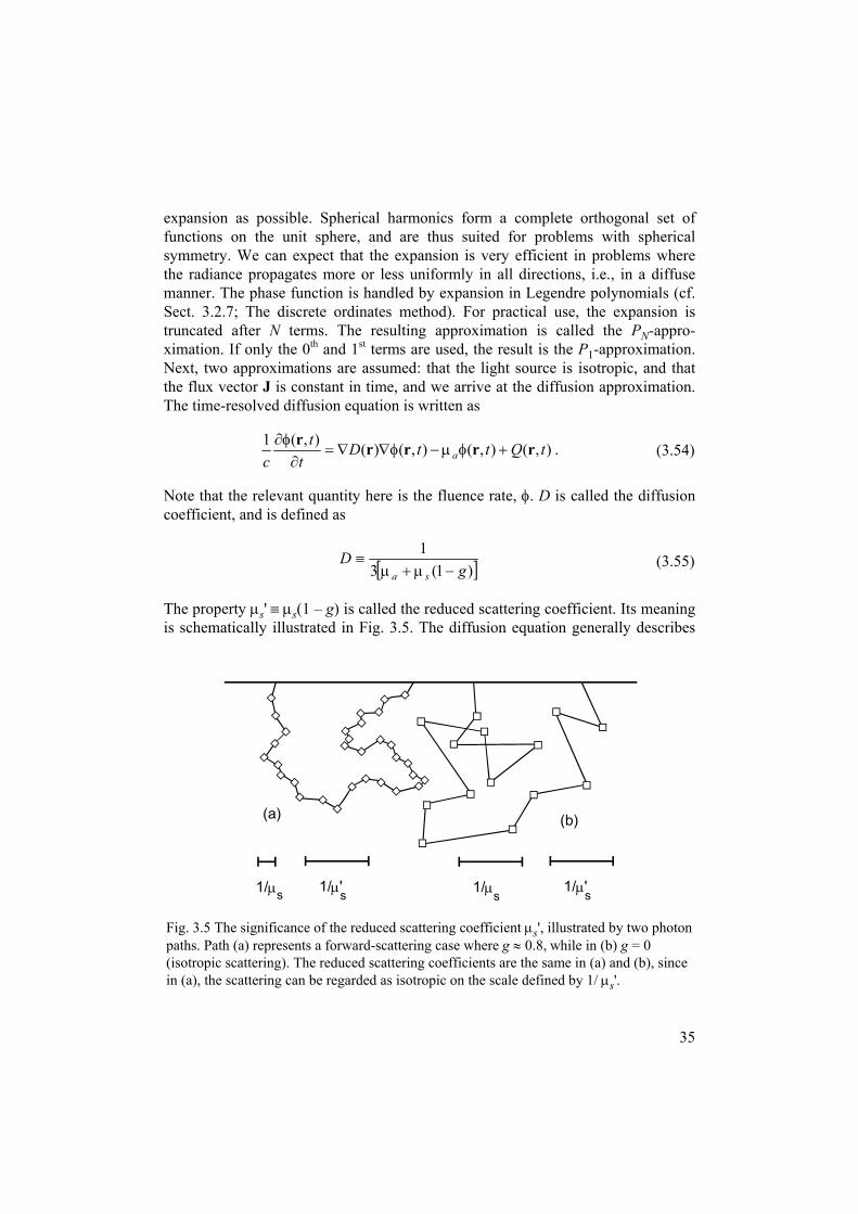
The property µs' ≡ µs(1 – g) is called the reduced scattering coefficient. Its meaningis schematically illustrated in Fig. 3.5. The diffusion equation generally describes
1/µs
(a)
1/µ's
Fig. 3.5 The significance of the reduced scatpaths. Path (a) represents a forward-scatterin(isotropic scattering). The reduced scatteringin (a), the scattering can be regarded as isotr
1/µs
(b)
1/µ's
tering coefficient µs', illustrated by two photong case where g ≈ 0.8, while in (b) g = 0 coefficients are the same in (a) and (b), sinceopic on the scale defined by 1/ µs'.
35
36
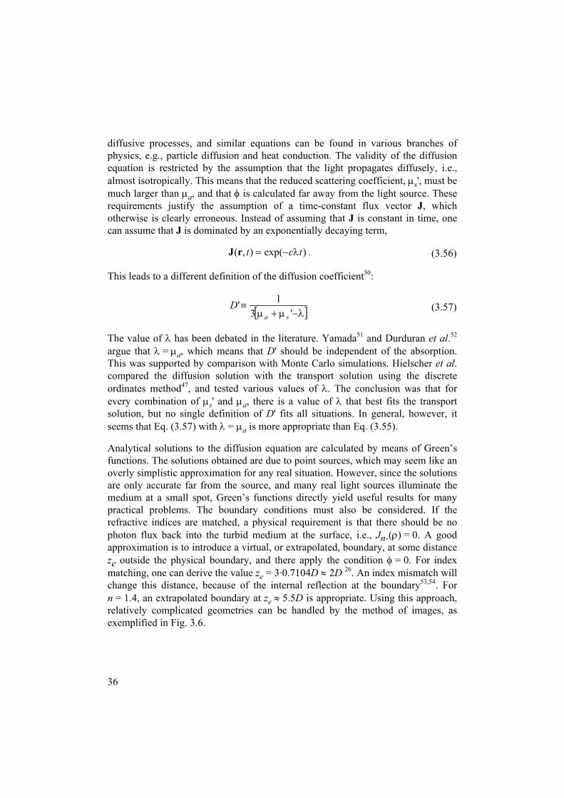
diffusive processes, and similar equations can be found in various branches ofphysics, e.g., particle diffusion and heat conduction. The validity of the diffusionequation is restricted by the assumption that the light propagates diffusely, i.e.,almost isotropically. This means that the reduced scattering coefficient, µs', must bemuch larger than µa, and that φ is calculated far away from the light source. Theserequirements justify the assumption of a time-constant flux vector J, whichotherwise is clearly erroneous. Instead of assuming that J is constant in time, onecan assume that J is dominated by an exponentially decaying term,
)exp(),( tct λ−=rJ . (3.56)
This leads to a different definition of the diffusion coefficient50:
[ ]λ−µ+µ≡
'31'
saD (3.57)
The value of λ has been debated in the literature. Yamada51 and Durduran et al.52
argue that λ = µa, which means that D' should be independent of the absorption.This was supported by comparison with Monte Carlo simulations. Hielscher et al.compared the diffusion solution with the transport solution using the discreteordinates method47, and tested various values of λ. The conclusion was that forevery combination of µs' and µa, there is a value of λ that best fits the transportsolution, but no single definition of D' fits all situations. In general, however, itseems that Eq. (3.57) with λ = µa is more appropriate than Eq. (3.55).
Analytical solutions to the diffusion equation are calculated by means of Green’sfunctions. The solutions obtained are due to point sources, which may seem like anoverly simplistic approximation for any real situation. However, since the solutionsare only accurate far from the source, and many real light sources illuminate themedium at a small spot, Green’s functions directly yield useful results for manypractical problems. The boundary conditions must also be considered. If therefractive indices are matched, a physical requirement is that there should be nophoton flux back into the turbid medium at the surface, i.e., Jn-(ρ) = 0. A goodapproximation is to introduce a virtual, or extrapolated, boundary, at some distanceze outside the physical boundary, and there apply the condition φ = 0. For indexmatching, one can derive the value ze = 3·0.7104D ≈ 2D 26. An index mismatch willchange this distance, because of the internal reflection at the boundary53,54. Forn = 1.4, an extrapolated boundary at ze ≈ 5.5D is appropriate. Using this approach,relatively complicated geometries can be handled by the method of images, asexemplified in Fig. 3.6.
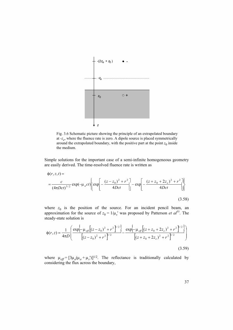
Simple solutions for tare easily derived. The
µ−π
=
=φ
Dctc
tzr
exp()4(
),,(
2/3
where z0 is the poapproximation for thesteady-state solution is
{[
−
π=φ
exp4
1),(D
zr
where µeff = [3µa(µa considering the flux ac
Fig. 3.6 Schematat -ze, where the around the extrapthe medium.
+
-
z
z0
-(2z + z )e 0
-ze
ic picture showing the principle of an extrapolated boundaryfluence rate is zero. A dipole source is placed symmetricallyolated boundary, with the positive part at the point z0 inside
37
he important case of a semi-infinite homogeneous geometry time-resolved fluence rate is written as
+++−−
+−−
Dctrzzz
Dctrzz
ct ea 4
)2(exp
4)(
exp)22
022
0
(3.58)
sition of the source. For an incident pencil beam, an source of z0 = 1/µs' was proposed by Patterson et al55. The
[ ] }]
[ ]{ }[ ]
+++
+++µ−−
+−
+−µ2/122
0
2/1220
2/1220
2/1220
)2(
)2(exp
)(
)(
rzzz
rzzz
rzz
rzz
e
eeffeff
(3.59)
+ µs')]1/2. The reflectance is traditionally calculated byross the boundary,
38
0)ˆ(),,(),0,(),(
=+ −⋅φ∇−=== zn tzrDtzrJtrR z (3.60)
which yields
−++
−µ−π=
=
−−
Dctr
zzDctr
zcttDc
trR
ea 4exp)2(
4exp)exp()4(
21
),(2
20
21
02/52/3
(3.61)
where r12 = z0
2 + r2 and r22 = (z0 + 2ze)2 + r2 for the time-resolved case. The
corresponding steady-state reflectance is written
µ−
+µ++
µ−
+µ
π= 2
2
2
202
1
1
10
)exp(1)2()exp(1
41)(
r
rr
zzr
rr
zrR effeffe
effeff (3.62)
Improved expressions for the reflectance can be obtained by instead taking theintegral of the radiance over the backward hemisphere. For n = 1.4, this leads tothe, more accurate, expression for the reflectance56:
),(306.0),0,(118.0),( trRtzrtrRimproved +=φ= (3.63)
Kienle et al. have derived a solution for a two-layer geometry, where the upperlayer has a finite extension, while the lower layer is infinite57,58. Analyticalsolutions for embedded spheres have also been derived59. A comprehensivetreatment on various analytical solutions of the diffusion equation is also presentedin Ref. 30.
For more complicated geometries, numerical methods are required to solve thediffusion equation. Two methods have been widely used: a finite-differencingmethod and a finite element method. Finite differencing (cf. Sect. 3.1.1) is astraightforward method, based on discretization of the diffusion equation and themedium. Usually, the Crank-Nicolson method is applied44. In three dimensions, themethod is called alternating direction implicit (ADI). This method is made efficientby iterating along one spatial coordinate at a time (“operator splitting”), whichmakes the inversion of the matrices simpler44,60,61. The drawback of the ADImethod is that the spatial grid is uniformly discretized, which is not optimal forgeometries that involve both large homogeneous regions and small complicatedinhomogeneities. This problem is solved by FEM, where the mesh spacing can beadapted to be crude for large structures and fine for small structures. General-purpose commercial FEM-packages like the FEMLAB toolbox for Matlab can be

39
used to solve the diffusion equation. FEM is well suited as a forward model forinverse problems, for other reasons in addition to the versatile mesh, as will bediscussed in Sect. 4.5; Optical tomography. Treating boundary conditions isusually not a problem for FEM since the computations always take place on closeddomains. FEM has been used by several researchers62-68.
As an alternative to deriving the diffusion equation for the P1-approximation, onecan derive the telegraph equation in the P1-approximation50,69. The flux J is thenallowed to vary in time, and the equation includes a second derivative in time. If Dis constant, the dependence of J vanishes and we have the homogeneous telegraphequation:
),(),(),(),()13(1),(3 22
2
2 tStDtt
tDct
tcD
aa rrrrr=φ∇−φµ+
∂φ∂
+µ+∂φ∂ (3.64)
The addition from the second derivative term is numerically small, and the result ofEq. (3.64) is very close to the ordinary diffusion equation, Eq. (3.54). A physicalinterpretation of this is that for diffusive propagation, the variation in J is slowcompared with the variation in φ, which is why one can assume that ∂J/∂t = 0 whenderiving Eq. (3.54).
The PN-approximation is discussed in Ref. 30 for higher values of N.
3.2.9 Probabilistic methods; Photon migration; Path integralsA random-walk type approach to treat light propagation in turbid tissue waspresented by Bonner et al.70,71. This model, like the diffusion approximation,assumes isotropic scattering. The method calculates the path-length distributions ofphotons re-emitted at arbitrary points on the surface. Following the ideas behindthis approach, the method of path integrals was introduced72-74. This method isbased on reformulation of the RTE, to solve for the path probabilities of photontrajectories in a non-absorbing medium. The usual radiometric quantities, such asthe radiance, can then be calculated using path integrals along the trajectories.
The term ‘photon migration’ is sometimes used to denote either, or both, of themethods just described, but often it just refers to light propagation in turbid mediain general.

40
3.2.10 The Monte Carlo methodMonte Carlo simulation owes its name to the famous casino, because the method isbased on, figuratively speaking, “throwing the dice.” The method relies on tracingindividual photon trajectories in a random walk fashion, where the scattering andabsorption events are governed by the probabilities given by µs and µa, as well asthe phase function p(s,s'). The key decisions to be made in a simulation are themean free path between scattering events, and the scattering angle. In addition, theabsorption of photons must be handled. The method is statistical and requires alarge number of photon histories to be computed. The number of photons neededdepends on the problem and the wanted accuracy.
Sampling random variables from non-uniform probability distributions is the coreof a Monte Carlo simulation. Let us denote a random variable x, which may be thestep size s to the next scattering event, or the scattering deflection angle θ. Thedistribution of x is described by a probability density function pp(x) over theinterval a ≤ x ≤ b:
1d)(p =∫b
ap xx (3.65)
The cumulative distribution function Fx(x1) describes the probability thata ≤ x ≤ x1:
∫=1
d)(p)(F 1
x
apx xxx (3.66)
Computers generate random numbers, here denoted ζ, in the interval [0,1], whichare uniformly distributed: pp(ζ) = 1. The distribution function in this case becomes
11
1
d)(p)(F ζ=ζζ=ζ ∫ζ
ζa
p . (3.67)
By letting a computer draw ζ, the method of sampling the variable x is to set Fx(x1)equal to Fζ(ζ1). The principle is illustrated in Fig. 3.7. This results in the importantequation
∫=ζ1
d)(p1
x
ap xx , (3.68)

which is thdistributionswe are readdeflection andefinition omedium betthe probabil
Integration o
In order for Eq. (3.68), a
Fig. 3.7arrows distribushaded
p(ζ)1
0
0
1
F (ζ)ζ
1
10
F (x)x1
0a b
p(x)
0a b
ζ
ζζ1
x
x x1
Sampling of a random variable from a non-uniform distribution. Theshow the mapping from the probability density function p(ζ), via thetion functions Fζ(ζ) and Fx(x), to the probability density function p(x). Theareas are equal, but shown in different scale.
41
e basic equation for sampling random variables from non-uniform using uniformly distributed random numbers. Now, using Eq. (3.68),y to derive how the random variables for step size s, scatteringgle θ, and scattering azimuthal angle ψ are sampled. According to the
f µs and µa, the probability of interaction per unit pathlength in theween s1 and s1 + ds1, is µtds1. This can also be expressed in terms ofities:
)()(d
d1
11 ssP
ssPst ≥
≥−=µ . (3.69)
f Eq. (3.69) yields
)exp()( 11 sssP tµ−=≥ . (3.70)
this result to be useful, we need the probability density function used innd we start by rearranging:
42
)exp(1)( 11 sssP tµ−−=< . (3.71)
We can directly identify this equation with the result of the integral in Eq. (3.68),so we disregard the step of differentiating Eq. (3.71) to get the probability densityfunction and then integrating back again. Thus, we have
)exp(1d)(p 10
1
1
sss t
s
p µ−−==ζ ∫ (3.72)
(we now drop the subscript 1:s for simplicity). Solving for s gives
ts
µζ−−
=)1ln( . (3.73)
Lastly, we substitute 1 – ζ → ζ, motivated by the fact that ζ is a random number inthe interval [0,1], and obtain
ts
µζ−
=)ln( . (3.74)
Note that Eq. (3.74) also shows that 1/µt can be interpreted as the mean free pathbetween photon interactions, since the statistical average of – ln(ζ), with thisdistribution of ζ, is equal to unity.
The scattering deflection angle θ is sampled from the Henyey-Greensteindistribution, Eq. (3.17). Inserting Eq. (3.17) in Eq. (3.68), and solving for cosθ,yields
ζ+−
−−+=θ
222
2111
21cos
gggg
g. (3.75)
Equation (3.75) is undefined for g = 0, so in the limit another expression is needed.g = 0 represents isotropic scattering, so p(cosθ) = ½ and the correct expressionbecomes
12cos −ζ=θ . (3.76)
Other phase functions are seldom used in Monte Carlo simulations within the fieldof tissue optics, but, e.g., the more general Reynolds-McCormick phase function33
can easily be incorporated with only slightly increased complexity:

43
++
ζα−+=θ
α−
α−
1
22 )1(2121cos g
Kgg
g, (3.77)
where α is an additional parameter and
αα
α
−−+−α
= 22
22
)1()1()1(2
ggggK . (3.78)
For α = 0.5 the Reynolds-McCormick function is equal to the Henyey-Greensteinfunction. Note that in general, g ≠ <cosθ> for the Reynolds-McCormick phasefunction.
The azimuthal scattering angle is uniformly distributed in the interval 0 < ψ < 2π,so we get
πζ=ψ 2 . (3.79)
Following from the definitions of µs and µa, the probability of absorption at anyphoton interaction site is µa/(µs + µa). Unless µa is very low, this implies that theprobability that a photon will survive more than a few scattering events is low. Thisleads to a problem in photon economy, in that a very large number of photons haveto be traced to yield acceptable accuracy at large distances from the source. Toimprove the accuracy for smaller number of photons, a variance reduction methodis used. Instead of terminating a photon at absorption, photon packets are launched,with initial weights W that can take on any number < W. This, effectively, is theequivalent of tracing a bunch of photons, which is reduced in number at everyscattering event. The weight should then be decreased by the amount
t
aWµµ
(3.80)
at every interaction point. Using this technique, the photon packet would be tracedforever (or until it escapes a boundary) unless there was some procedure forterminating the trajectory. The termination method is called the roulette. At somepoint, W is so low that the photon packet contributes little to the simulation. Whenthe weight falls below this threshold value, e.g., 1:1000, there is a one in m chancethat the photon packet will survive the roulette procedure. In case it survives, itsweight is increased m times, otherwise it is terminated. In this way, the totalamount of launched energy in the simulation is conserved.
44
The number of photon packets needed for a simulation depends on the geometryand the quantity of interest in the problem. For example, to compute the totalreflection from a semi-infinite medium, only about 5000 photons may suffice, andthe simulation takes less than a second on a PC. To compute the spatial distributionat different radial distances from the source, at least an order of magnitude morephotons are needed. Time-resolved data at distances more than 1 cm from thesource (for optical properties typical of tissue) needs tens of millions of photons toyield acceptable statistics.
Computer code for Monte Carlo simulations is easy to write using the guidelinesabove, however, since speed is imperative, a good knowledge of programming atboth machine and programming language level is necessary to write efficient code.The finished code should also be validated thoroughly. An important point is therandom number generator, which, in computers, usually is in the form of a pseudo-random number generator. Since very long sequences of random numbers areneeded, it is essential that the pseudo-random numbers are sufficiently random in astatistical sense, and that the sequence does not repeat itself. Computer-generatedrandom numbers have been discussed in Refs. 44 and 75. The program MonteCarlo simulation for Multi-Layered media, MCML, by Jacques and Wang76,77, hasbecome somewhat of a standard in the field of tissue optics. The program waswritten in C. All simulations performed in this thesis were done using codes basedon MCML. An adaptation to time-resolved data and more complex geometries wasimplemented by Berg78, but the photon propagation routines are the same for allsubsequent versions of the program.
3.2.11 Variations on Monte Carlo simulationsIn addition to the extended time-resolved version of MCML mentioned in theprevious section, other variations on Monte Carlo simulations have been explored.The phase function, which typically is sampled from the analytical Henyey-Greenstein distribution, can instead be incorporated in the simulations usingscattering patterns computed with Mie theory or T-matrix theory. Phase functionstaken directly from T-matrix computations have been used with MCML within ourgroup79.
Another powerful approach is the so-called white Monte Carlo method. Theamount of computations needed for Monte Carlo simulations can be reduced byperforming only one simulation with µa = 0, and then adding the absorptionafterwards using the Beer-Lambert law. The number of free parameters is thenreduced to two: µs and g. In case the medium is homogeneous and infinite or semi-infinite, the method is especially powerful, since then it is possible to rescale µs by
45
rescaling the spatial coordinates. The g-factor can often be considered constant,and thus only one single simulation is necessary to yield solutions for allcombinations of µa and µs
80,81.
An important question is whether the white Monte Carlo method is equivalent tothe conventional approach. The conventional step size is, on average,1/µt = 1/(µa+µs), while it is 1/µs with the white method. This will result in differentphoton distributions. The photon weights are also handled differently. Using theconventional procedure, the photon weight is decreased according to Eq. (3.80) ateach interaction. After N steps, the photon packets have, on average, traveled adistance d = N/µt, and the weight is
N
t
ad WW
µµ
−= 1 , (3.81)
where W is the initial weight. After the same distance, for a corresponding whitesimulation, the weight would be
µµ
−=t
ad NWW exp (3.82)
(note that N still stands for the number of steps in the conventional simulation – inthe white simulation the number of steps would be different).
First, let us consider the extreme cases, and start with when the albedo a → 1.Now, the average step sizes of the two approaches become equal, and Eq. (3.82) ismathematically equivalent with Eq. (3.81). Clearly, the white approach isequivalent with the conventional in this limit. This is the regime usuallyencountered in tissue optics problems. In the other extreme, a → 0, which meansno scattering. Physically, this case is described by Beer-Lambert’s law for a purelyabsorbing medium. In the conventional method, the photon paths are now given bys = ln(ζ)/µa, and the photons are absorbed at the first interaction site. This isstatistically equivalent with Beer-Lambert’s law. In the white approach, the stepsize s → ∞, but the photons are in practice always terminated due to interactionswith interfaces or a detector. The weights are then updated according to Beer-Lambert’s law, and it is clear that again the conventional and the white approachesare equivalent.
In the intermediate regime, when µa ≈ µs, equivalence is not guaranteed because ofthe difference between the functions in Eqs. (3.81) and (3.82). A practical exampleillustrates this. In Fig. 3.8 (a), the results of simulations, using each method, areshown. The spatially resolved reflectance is depicted as a function of the radial

10-10
10-8
10-6
10-4
10-2
100
Ref
lect
ance
(nor
mal
ized
)
1086420Radial distance (mm)
Conv. MC, µa = 10 cm-1
White MC, µa = 10 cm-1
Conv. MC, µa = 20 cm-1
White MC, µa = 20 cm-1
10
8
6
4
2
0
Rat
io o
f Con
vent
iona
l/Whi
te
1086420Radial distance (mm)
µa = 10 cm-1
µa = 20 cm-1
Fig. 3.8 Comparison between the conventional and the white Monte Carlo method. The inputparameters were µa = µs = 10 cm-1 in the first case, and µs = 10 cm-1, µa = 20 cm-1 in thesecond. The anisotropy factor was g = 0.5. A total of 106 photon histories were traced for theconventional method, and 105 for the white method. In (b), the ratio between the methods ispresented.
46
distance from a point source on the surface of a semi-infinite medium. The opticalproperties were, in the first case, µa = µs = 10 cm-1, g = 0.5, and in the second case,µa = 20 cm-1, µs = 10 cm-1, g = 0.5. The ratio between the two methods is alsopresented in Fig. 3.8 (b), which reveals that the difference is a constant factor,however dependent on the properties µa and µs.
The white Monte Carlo method has been shown to provide accurate results fortissue optics problems80-83, and was also used in Paper I.
Transport theory in the form described by the RTE, Eq. (3.7), does not account forany of the wave characteristics of light, such as coherence, interference effects orpolarization. It is, however, possible to introduce a description of polarization usingthe Stokes vector formalism. The scalar radiance must then be replaced by a vectorwhose components are the Stokes parameters for radiance26. This extension isespecially well suited for Monte Carlo simulations. The polarization becomes aparameter to be logged for each photon packet, described by the Stokes vector, andthe depolarization due to scattering is an additional optical property of the turbidmedium, given by the Mueller matrix for each scattering event. A polarizationMonte Carlo code has been developed by Wang and co-workers84, based on theMueller-Stokes formalism, where the Mueller matrix is calculated from Mietheory. Birefringent media are also possible to simulate85.
47
3.2.12 Time-resolved and frequency-resolved calculationsSo far in this treatment, frequency-resolved calculations have not been discussed.By frequency-resolved calculations, a procedure where the amplitude of the lightsource is sinusoidally modulated at a certain frequency is meant, and the detectionis performed at the same frequency. From a mathematical perspective, time-resolved and frequency-resolved calculations are equivalent, coupled by theFourier transform. In some instances, performing the calculation in either domainmay be advantageous for numerical reasons, and then the other solution can beobtained by transformation using the Fast Fourier transform (FFT).
In the frequency domain, the propagating light may be conceptually visualized asphoton density waves. Care should be taken not to push this picture too far – thephoton density is for example always positive and interfering photon density wavescan therefore never cancel each other out in the traditional sense, but instead, themodulation becomes zero. The spatial characteristics of photon density waves arealso somewhat different from the usual conception of waves, since the fluence ratealways obeys φ(r1) > φ(r2) for all distances from the source r1 < r2 for diffusepropagation. One may define wavelength, amplitude, and phase properties forphoton density waves.
More aspects on frequency-resolved vs. time-resolved measurements are discussedin Sects. 5.3.2 and 5.3.3; Instrumentation.
3.2.13 Fluorescence and inelastic scatteringFluorescence may be widely defined as a process where light energy is absorbedand re-emitted at a different wavelength than the original light. For the purpose ofthis thesis, this is as detailed an explanation as is necessary. In a light transportproblem, fluorescence phenomena add complexity, but no fundamental newphysics. The basic approach to a description of fluorescence within transport theoryis to regard the propagation of the excitation light and emission light as twodifferent problems, and find a way to handle the transition of excitation light tofluorescence light. Various Monte Carlo models on this theme were developed inPaper I.
Fluorescence spectroscopy of tissues is a very vivid field of research aiming atdeveloping modalities for diagnostics. Reviews of this research are presented in,e.g., Refs. 86 and 87.
To the level of sophistication of the description presented above, inelasticscattering processes, such as Raman scattering, are treated identically tofluorescence processes. The difference is that while the fluorescence process
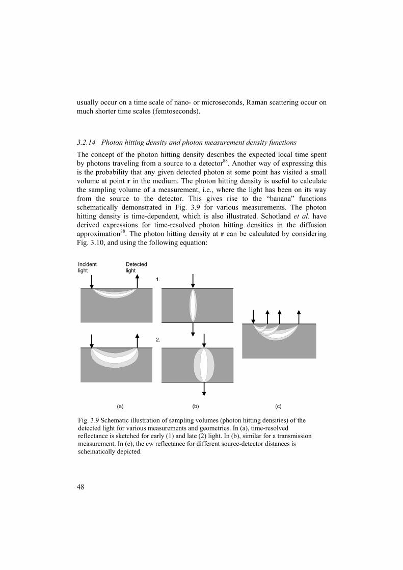
usually occur on a time scale of nano- or microseconds, Raman scattering occur onmuch shorter time scales (femtoseconds).
3.2.14 Photon hitting density and photon measurement density functionsThe concept of the photon hitting density describes the expected local time spentby photons traveling from a source to a detector88. Another way of expressing thisis the probability that any given detected photon at some point has visited a smallvolume at point r in the medium. The photon hitting density is useful to calculatethe sampling volume of a measurement, i.e., where the light has been on its wayfrom the source to the detector. This gives rise to the “banana” functionsschematically demonstrated in Fig. 3.9 for various measurements. The photonhitting density is time-dependent, which is also illustrated. Schotland et al. havederived expressions for time-resolved photon hitting densities in the diffusionapproximation88. The photon hitting density at r can be calculated by consideringFig. 3.10, and using the following equation:
Incident light
Detectedlight
(a) (b) (c)
1.
2.
Fig. 3.9 Schematic illustration of sampling volumes (photon hitting densities) of thedetected light for various measurements and geometries. In (a), time-resolvedreflectance is sketched for early (1) and late (2) light. In (b), similar for a transmissionmeasurement. In (c), the cw reflectance for different source-detector distances isschematically depicted.
48

∫τ−
τ
−φ=ν2
1
'd)';,()';,();,;( 2121
t
tttEtt rrrrrrr , (3.83)
where φ is the fluence rate at r due to a source a r1, and E is the escape functionfrom r to a detector at r2. The concept of photon hitting density was generalized toany type of measurement by Arridge, under the name photon measurement densityfunctions89. Photon measurement density functions are a measure of the sensitivityof a measurement with respect to small changes in the optical properties50,89. Assuch, they play an important role in reconstruction methods, since they can be usedto build the Jacobian matrix in the optimization problem (cf. Sect. 4.5; Opticaltomography).
Monte Carlo simulation is a convenient way of obtaining photon hitting densitiesfor arbitrary geometries, since the ensemble of photon trajectories directly yield thephoton hitting density. The problem with the Monte Carlo method, however, is itsslowness. In Paper I, a variance reduction technique was utilized to improve theefficiency of fluorescence Monte Carlo methods. It was based on separating thecomputation of the excitation light and the fluorescence light, and furthermore,reversing the computation of the fluorescence light by means of the reciprocityprinciple. In an analogous fashion, it would be possible to compute the photonhitting density more efficiently by reversing the computation of the escape functionE and applying the convolution method in Eq. (3.83). Another option for complexgeometries is to use FEM to solve the diffusion equation. Arridge and Schweigerhave implemented this in connection with tomographic reconstruction, and utilizethe reciprocal computation (they call it the “adjoint” problem) to compute theescape function in their FEM model50,65.
Fig. 3.10 Parametelimits for t' are alsreach r, and the las
(r ,t=0)
(r,t')
(r ,t)
cr
ttc
−−<<
− 21 rrr'
12
rs for the definition of the photon hitting density. The integrationo shown, which are defined by the time it takes for the first light tot light to leave r in order to reach r2 at time t, respectively.
49

50
3.3 Discussion – solving the forward problemIn the previous sections, a map of various methods to solve the forward problemhas been presented. The method of choice for a particular problem is sometimesobvious, but, often, tradition and familiarity governs what method people choose,even though it might not be the optimal choice. Here, we will discuss some generalproperties of the most widely used methods, and compare them with each other.Often, the method is to be used as a means to solve the inverse problem, which isthe topic of next chapter. Therefore, this discussion should also be taken as astarting point for the review of inverse methods in the next chapter.
The diffusion approximation is probably the most widely used method in tissueoptics. The method has many attractive properties. Analytical solutions exist forseveral geometries that are useful in practice. Numerical computations using finite-differencing schemes or FEM are conveniently manageable on personal computers.The diffusion equation directly gives the fluence rate everywhere in the medium,which makes it simple to calculate the absorbed dose, by multiplication with theabsorption coefficient, Eq. (3.14). Diffusion theory is therefore often used for dosecalculations. The obvious drawback of the method is the restricted validity: therequirement µa << µs', and that the solutions are inaccurate close to the source.Many complex media consist of different regions, some with high µs' where thediffusion approximation is perfectly valid, but others where the scattering is low. Insome cases, high absolute accuracy is not a great concern, and in such situationsthe method can still be useful. An example is reconstruction in optical tomography,which will be discussed in more detail in Sect. 4.5.
The discrete ordinates method and the Monte Carlo method are similar in the sensethat both, in principle, solve the RTE accurately without approximations orlimitations. These methods are based on entirely different principles, but bothconsume large amounts of computer power. The Monte Carlo method is preferredwhenever the distance between the light source and detector is small. The numberof photons required for acceptable accuracy increases exponentially with thedistance, so at distances larger than a few hundred mean free paths (2 – 3 cm intypical tissue), the computation time becomes unrealistic. Discrete ordinatescomputation time is proportional to the grid size, i.e., to the number of mean freepaths cubed, so although the computation requires powerful computers, it may stillbe realistic to perform a discrete ordinates calculation in situations when the MonteCarlo method is impossible.
The Monte Carlo method, thanks to its high accuracy, has gained a position as areference method that other methods are measured against. A large number ofmodels based on diffusion theory have been validated by means of Monte Carlosimulations 53,56,90-100. Several authors have also presented hybrid models, where the

51
region close to the source is modeled using Monte Carlo simulations, while in thediffusive region far from the source diffusion theory takes over92,98,99.
3.3.1 Relationship between wave theory and transport theoryThe relationship between electromagnetic wave theory and transport theory is aquestion of fundamental interest. The two theories represent two different views oflight propagation on different levels of description. However, a link between thesetwo levels have already been discussed in connection with the phase function,which can be calculated using, e.g., Mie theory, and incorporated into transportmodels. The relation between wave and transport theory has been discussed byFante101 and Ishimaru26. Their analysis shows that the quantity radiance, as used intransport theory, can be regarded as a statistical average of the time-varyingPoynting vector in wave theory, and thus that there exists a formal link between thetwo theories.
Links between the wave and transport representations are important for practicalreasons as well. In the transport models, the scattering properties can only bemeasured; there is no way of calculating the scattering coefficient from knowledgeof the composition of the medium. The simple example of scattering microspheresshows how the scattering coefficient can be calculated using wave theory, and thenbe applied in a transport model. In some media, the transport scattering coefficientchanges dramatically due to microscopic configurational changes. An example isblood, which was studied in Papers V and VI. The only way to predict thecomplicated variation of the scattering coefficient in blood under differentconditions is by means of applying wave theory on the scattering problem on themicroscopic level. Another example is when polarization effects are included intransport models. Within the context of transport theory, depolarization of anincident light beam is a property that can only be measured. On the other hand,using for example Mie theory, it is relatively easy to calculate the depolarization inconnection with scattering from spherical particles84.

52
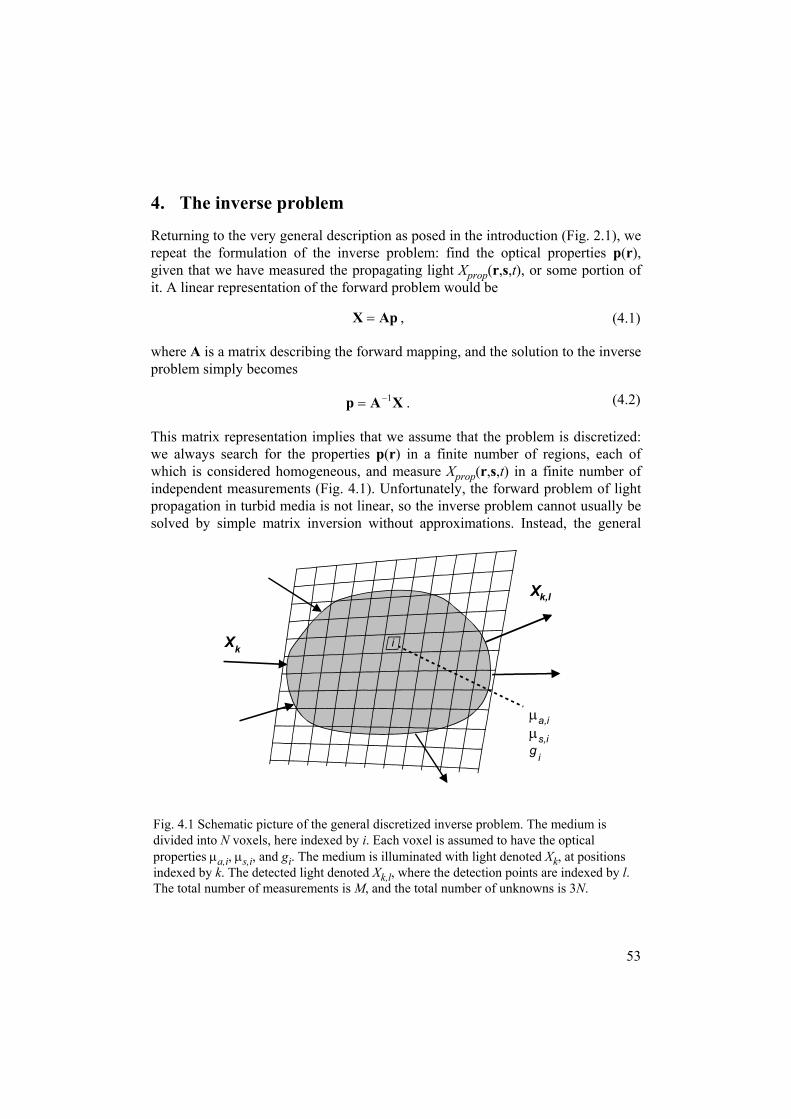
4. The inverse problem
Returning to the very general description as posed in the introduction (Fig. 2.1), werepeat the formulation of the inverse problem: find the optical properties p(r),given that we have measured the propagating light Xprop(r,s,t), or some portion ofit. A linear representation of the forward problem would be
ApX = , (4.1)
where A is a matrix describing the forward mapping, and the solution to the inverseproblem simply becomes
XAp 1−= . (4.2)
This matrix representation implies that we assume that the problem is discretized:we always search for the properties p(r) in a finite number of regions, each ofwhich is considered homogeneous, and measure Xprop(r,s,t) in a finite number ofindependent measurements (Fig. 4.1). Unfortunately, the forward problem of lightpropagation in turbid media is not linear, so the inverse problem cannot usually besolved by simple matrix inversion without approximations. Instead, the general
Fig. 4.1 Scdivided inpropertiesindexed byThe total n
Xk
µa,iµs,ig
Xk,l
i
i
hematic picture of the general discretized inverse problem. The medium isto N voxels, here indexed by i. Each voxel is assumed to have the optical µa,i, µs,i, and gi. The medium is illuminated with light denoted Xk, at positions k. The detected light denoted Xk,l, where the detection points are indexed by l.umber of measurements is M, and the total number of unknowns is 3N.
53

54
approach fin Fig. 4.2to the forwthe measurupdated. Tmatch withas the final
In this chaproblem. Toften the nregion, butthe thicknconsideredof optical attemptingstructure omethod fomedium. T
Fig.an it
startp
Forward model
computedX
Match?measuredX
resultp
Compute δp
ppp δ+←
Yes
No
The forwardproblem
Theoptimizationproblem
4.2 The principle of solving a non-linear inverse problem by means oferative algorithm.
or non-linear inverse problems is iterative. This procedure is illustrated. The process is started by guessing initial values of p(r), which are fedard model. The computed values of Xprop(r,s,t) are then compared withed, and using a suitable minimization algorithm the values of p(r) arehe process is repeated until the computed and the measured valuesin required accuracy, at which point the current values of p(r) are taken result.
pter, we will focus on some of the more important aspects of the inversehe first consideration is the number of unknowns in the problem. This isumber of spatial regions times the number of optical properties in each sometimes there are also geometrical parameters as unknowns, such asess of a layer. An important special case is when the medium is homogeneous, and the number of unknowns is reduced to the numberparameters. When the number of spatial regions is large, what we are is effectively three-dimensional mapping, or imaging, of the internalf the turbid medium. The ultimate goal of this branch of tissue optics is ar complete reconstruction of the optical properties at every point in thehis topic is covered in the section on optical tomography, Sect. 4.5.

55
The first choice is which forward model to use. Methods based purely onelectromagnetic wave theory have never really been applied to inverse problems incomplicated turbid media, due to the computational requirements. Mie theory canbe used to characterize the properties of aerosols by measuring the scatteringpattern. Determining the geometry of aircraft from radar signals is another inverseproblem of this kind, albeit more complicated. In Paper V, an attempt was made toexplain the optical response from whole blood by means of T-matrix calculations.However, the comparison was mainly qualitative, and the model cannot at presentbe used as a forward model for the inverse problem. In the following treatment,only models based on transport theory will be considered.
Next, the type of measurement is an important factor. Ideally, the number ofmeasurements should equal the number of unknowns, and they should all beorthogonal in measurement space. In reality, the inverse problem is often illconditioned – some measurements are almost parallel in measurement space, and inthe case of imaging the number of measurements is smaller than the number ofunknowns. In image reconstruction, regularization methods are used to handlethese problems. For measurements of homogeneous media, the way to handle ill-conditioned inverse problems is usually by one or several of the followingmethods: (A) choose the measurement carefully to avoid or minimize the ill-conditioned inverse; (B) minimize noise and errors in the measurement; (C) useappropriate numerical methods to handle ill-conditioned problems.
The third part is the choice of optimization method. Many minimization algorithmsuse the derivative, or an estimation of the derivative, to calculate the step δp thatp(r) will change in each iteration. Examples of standard algorithms are thedownhill simplex method (which does not require the use of the derivative) and theconjugate gradient method (which does use derivatives)44. For imagereconstruction, efficient minimization routines are even more important because ofthe high computational cost of evaluating the forward model for complicatedgeometries; as few iteration steps as possible is desirable. This topic will bediscussed more in Sect. 4.5.
4.1 Two-parameter methodsThe lowest number of unknowns possible is N = 1, meaning that only either thescattering or the absorption is unknown. The other parameter is then assumedknown. We will, however, start the discussion with two-parameter methods, whereboth the reduced scattering µs' and the absorption µa are unknowns, and themedium is assumed homogeneous. An important fact immediately comes up: it isnot possible, using any two-parameter method, to measure µs. Either µs' is

measured, or both µs and g are measured, the latter which renders the method athree-parameter method. Two-parameter methods are based on measurements ofthe diffuse reflectance or transmittance from the medium, which can be spatiallyresolved, time-resolved or frequency-resolved. These three methods are depicted inFig. 4.3. The bulk refractive index of the medium is assumed to be known in thesemethods.
(a) (b) (c)
r dr
dr
R
r t
R or TInjected pulse
Detected pulse
A
B
C
D
ϕ
Source
Detected signal
t
R or T
Fig. 4.3 Three types of measurements to obtain the two parameters µs' and µa. (a) Cwspatially resolved reflectance measurement; (b) time-resolved measurement by injecting ashort pulse and measuring the temporal point-spread function (either reflectance ortransmittance mode); and (c) frequency-modulated measurement (either reflectance ortransmittance mode). In (c), the phase shift ϕ and the modulation depth = (C/D)/(A/B) aremeasured.
56
4.1.1 Spatially resolved diffuse reflectanceSpatially resolved diffuse reflectance measurements based on continuous wave(cw) light can be evaluated by fitting the measurement, R(r), with the diffusionequation, Eq. (3.62). A measurement of R(r) generally leads to an over-determinedinverse problem, since only two values, R(r1) and R(r2), in principle are necessary.The optimal distances r1 and r2, in the sense that the measurements are orthogonal,can be found by considering Fig. 4.4. The “hinge” and “pivot” points indicate the

distances of invariance in terms of µa and µs', respectively. Typically, for opticalproperties that are relevant for biological tissue, r1 ≈ 0, while r2 ≈ 3 mm102. Inpractical situations, measuring at more than two positions is sensible, to make themethod more robust with respect to measurement errors or small inhomogeneitiesat the measurement position. Since measurements close to the light source arenecessary to obtain orthogonal measurements, the diffusion equation is not an idealforward model. Still, several authors have shown good results using the diffusionequation103-106. Alternatives to the diffusion equation are to use the Monte Carlomethod107, or simply to calibrate the measurement on phantom samples with knownoptical properties102. The latter method requires the use of a non-linear calibrationmethod (cf. Sect. 4.4).
Spatially resolved measurements proinstrumentation can be made inexpmeasurements can be done in vivo on pfairly sensitive to inhomogeneities in theprobes different volumes, at different delight source (cf. Fig. 3.9). Secondly, measurement is susceptible to small inhclose to the measurement site. The latteseveral positions along concentric circleover the angle ψ102,107. An additional limis that deep structures inside the medium
µ
R
r
a
Hinge(a)
Fig. 4.4 Spatially resolved reflectance R(invariance, the “hinge” point, is close to “pivot” point marks the point of invarian
µ'
R
r
s
Pivot
(b)
r). In (a), µa is varied and the point ofthe source. In (b), µs' is varied and thece. Adapted from Dam129.
57
vide several attractive properties: theensive, small and portable, and theatients. A drawback is that the method is medium, for two reasons. Firstly, the lightpths, depending on the distance from thesince the cw intensity is measured, theomogeneities, such as an absorbing spot,r can be partly overcome by measuring ats around the light source, and integratingitation of spatially resolved measurements are inaccessible.

58
4.1.2 Time-resolved diffuse measurementsTime-resolved measurements are performed by using short light pulses, in thepicosecond regime, and measuring the temporal point-spread function (TPSF) atsome distance from the injection point. The standard way of evaluating thesemeasurements is by fitting with the diffusion equation, Eq. (3.61). Diffusion theoryis well suited for this problem, since the distance between the source and thedetection point can be kept rather large. The fitting is performed with a non-linearcurve-fitting algorithm, e.g., the Levenberg-Marquardt method44,108. In an analogywith the spatially resolved measurements, in principle only two values from theTPSF are necessary to deduce µs' and µa. In rough terms, the early part of the TPSFcurve is invariant with respect to µa, while the tail is invariant with respect to µs'. Infact, a reasonably good estimation of µa can be obtained by simply measuring theslope of the trailing edge in a lin-log graph, as can be seen from the exponentialexpression in Eq. (3.61).
Although diffusion theory is often adequate as the forward model, sometimes onewishes to measure with short source-detector distances. The Monte Carlo methodthen useful. The problem is the computation time required when the Monte Carlomethod is incorporated in an iterative scheme like in Fig. 4.2. The computationtime can be reduced substantially by applying the white Monte Carlo method (Sect.3.2.11). Only one simulation is then necessary, and the fitting can be performed byrescaling the curve and adding absorption80,81.
Time-resolved measurements solve some of the problems associated with spatiallyresolved cw measurements. The method is less sensitive to small inhomogeneities,since only the shape of the TPSF curve and not the absolute intensity is used. Asmall absorbing spot close to the detection point will thus only act as a gray filter,and reduce the amplitude of the TPSF. The method is also ideal for measurementsof large volumes, as long as the intensity of the light is high enough to be detected.The major drawback of the method is the expensive and complicatedinstrumentation (cf. Sect. 5.3.3; Instrumentation). Like spatially resolvedmeasurements, time-resolved measurements are ideal to perform in vivo.
Measurements with sinusoidally amplitude-modulated light are mathematicallyequivalent with time-resolved measurements. Expressions that directly link themeasured phase and modulation from frequency-resolved measurements to µs' andµa have been developed, based on diffusion theory109,110.

4.2 Three-parameter techniques; The integrating sphere method
An elegant way of determining all three optical properties – µs, µa and g – ispresented by the integrating sphere method. The technique requires small samples,which may be an advantage in some situations, but usually it is the main limitationof the integrating sphere method, since in-vivo measurements of tissue areimpossible. An integrating sphere is designed to collect all light flux that enters thesphere, and a portion of it, α, is detected by a detector that is mounted at a positionon the sphere wall. The samples are cut into thin slabs (usually around 1 mm forbiological tissue), which can be placed either at the entrance port or the exit port ofthe sphere (see Fig. 4.5). The sample is illuminated by a collimated light beam thatis aligned with the optical axis of the two ports of the sphere (other measurementgeometries are possible, e.g., diffuse illumination of the sample111,112). This set upenables measurement of the transmittance (T) and reflectance (R) of the thinsample. When the transmittance measurement is performed, the exit port is coveredwith a calibrated plug with known (high) reflectance, Rref. A referencemeasurement is carried out with no sample, which yields a measure of the
Detector
Referencesample
Sample Sample
Referencesample
Entranceport
Exitport
(a) (b)
(c) (d)
Fig. 4.5 Integrating sphere measurements. (a) shows the basic set-up, with a collimatedbeam along the port axis of the sphere. This is also used to perform backgroundmeasurements. In (b), a reference measurement is performed on a calibrated sample whichyields αE0. In (c), the transmitted signal αET is measured. Finally, in (d), the reflectedsignal αER is measured.
59

60
unattenuated beam, αE0. From the sample measurements, αET and αER, thetransmittance and reflectance can be calculated as
00 EE
EET TT =
αα
= (4.3)
and
00 EE
REE
RR Rref
Rref =
αα
= . (4.4)
So far, the method described is a two-parameter method: knowledge of R and T issufficient to determine µs' and µa. In this way, the integrating sphere method wasused in Paper V to measure the optical properties of flowing whole blood. Todetermine the g-factor, and thus separate µs' in µs and g, a third measurement isnecessary. The usual procedure is to measure the collimated transmittance andderive µt using Beer-Lambert’s law, Eq. (3.36). The three parameters, R, T and µt,are sufficient to give a reasonably well-conditioned inverse problem.
To solve the inverse problem, the adding-doubling method has been usedextensively as the forward model112-114. Adding-doubling provides quickcomputations, but suffers from an important weakness. In practice, there are alwayslateral losses of light due to the finite size of the sample and/or integrating sphereports. Such losses lead to underestimation of R and T compared with the ideal case,which in turn lead to overestimation of the absorption properties of thesample115,116. Another approach is to use the Monte Carlo method, where the laterallosses easily can be incorporated in the model. The problem with Monte Carlosimulations is again the long computation time. To overcome this, one can computea database of values of R and T which spans the region of µs, µa and g of interest,and then interpolate in this database to find the correct values117-119. The solution ofthe inverse problem is thus transferred to a method of using look-up tables. Theinterpolation algorithm can be made in different ways, e.g. by using splineinterpolation117-120, which was applied in Papers V and VI, or by means of apolynomial regression technique121. The latter method has proved to be superior,and was used in Papers II and IV. The polynomial regression technique isdescribed in more detail in Sect. 4.4.
Several sources of error have to be considered when performing integrating spheremeasurements. One type has to do with the sphere itself, and occur because theratio between the area of the various ports of the sphere and the total area of thesphere is not zero. Fundamental integrating sphere theory has been treated byseveral authors111,122-124. The most influential sphere error occurs in the

measurement of the transmittance. The sphere geometry is affected slightly byintroducing the sample at the entrance port, so that the sample itself can reflectsome of the light inside the sphere. The reference measurement, taken withoutsample, should therefore be corrected. An alternative, superior, to Eq. (4.3) forcalculating T is given by
[ ]{ }[ ][ ])1(1)1(
)1(1)1(
0 swsws
swswsT
RRRRRR
EE
Tε−−ε+ε−
ε+ε−−ε−= , (4.5)
where εs is the ratio of the sample port to the total sphere area, and Rw is thereflectance of the sphere wall124. An example of the correction factor comparedwith Eq. (4.3), for the sphere used in the experiments in this thesis (Papers II, IV –VI) is shown in Fig. 4.6. The correction in Eq. (4.5) can be improved further byincorporating effects due to the fact that some of the transmitted light is stillcollimated, but this correction is small compared with Eq. (4.5)125.
The correctiused simultaThe double simultaneoufactors for diffusely tradegraded whmethod shou
Fig. 4.6 CoThe sphere
1.00
0.98
0.96
0.94
0.92
0.90
0.88
0.86
T co
rrect
ion
fact
or
1.00.80.60.40.20.0R
rrection factor for T according to Eq. 4.5, for the sphere used in this thesis.properties were εs = 0.0035 and Rw = 0.97.
61
on factors become more important when two integrating spheres areneously, because of cross talk through the sample between the spheres.integrating sphere set up has been used as a means to provide
s measurement of R and T 111,112,114,118. However, the derived correctionthe double integrating sphere are dependent on the assumption ofnsmitted and reflected light from the sample, and the accuracy isen this requirement is not fulfilled. The double integrating sphereld therefore be used with caution.

62
The next important potential source of error has already been mentioned: laterallosses of light due to the finite size of the ports. This leads to overestimatedabsorption properties for samples with low absorption115,116. The losses can easilybe 5% for a typical measurement on a sample with low absorption, which meansthat R + T ≈ 0.95 instead of the true R + T ≈ 1. The lateral losses can be correctedwhen the Monte Carlo method is used for evaluation. Measurement of lowabsorption coefficients is, in general, a weak point of the integrating spheretechnique, even if the above corrections are included. The absolute error in theevaluation of µa is directly determined by the error in the measurement of R and T.If µa is small, even an error as small as 1% in the measurement will lead to relativeerrors of several hundred per cents in µa.
The collimated-beam measurement has its own potential sources of error. Thefundamental idea behind this measurement is to detect only the light that haspenetrated the sample without being scattered. Ideally, this implies measuring in azero collection angle. In practice, the measured signal is proportional to
scatteredcolmeas EEE ε+= , (4.6)
where ε is the fraction of the scattered light that falls inside the collection angle ofdetection. Suppressing the scattered light in the set up is imperative, but at somepoint the fraction of scattered light can no longer be neglected. The error increaseslinearly with sample thickness and scattering coefficient, quadratically with thecollection angle, and is inversely quadratically proportional to (1 – g) and therefractive index of the sample126. In practice, the range of possible measurementscan be increased either by making the samples thinner, or increasing the radianceof the light source to enable a smaller collection angle of the detector. Before anycollimated attenuation measurements can be trusted, a thorough characterization ofthe experimental set-up must be performed. This is done by recording Emeas for aseries of samples with known values of µt, and then plotting these in a lin-log graphto determine the linear range, and upper threshold value of µt for which themeasurements are relevant. The dynamic range of the measurement with thesample compared with the reference measurement is also a problem, which can besolved by using neutral density filters for the latter measurement. This waspracticed in Papers II and IV.
Using a laser for the collimated beam measurement would seem ideal, because ofthe high radiance. Unfortunately, the high coherence of most lasers introduce othererrors in the measurement. The sample is usually placed in a glass cuvette, orclamped between two glass plates. When using a high coherence light source,interference effects in the glass plates can cause large variations in the detectedsignal.
63
The collimated beam measurement can be combined with the double integratingsphere for simultaneous measurement of all three parameters. However, in thissituation, some of the scattered light from the sample will reflect off the wall of thesecond sphere, reflect again off the sample and interfere with the measurement.The problems associated with this kind of measurement have been discussed inRef. 120. The conclusion was that often only relative measurements of the opticalproperties are possible using this set up, due to the errors. This can, in someinstances, be a price worth paying for the benefit of being able to measure all threeproperties simultaneously.
The integrating sphere method is ideal for situations where destructive testing canbe tolerated. It has been used on paper, plastics, and other materials. Oneinteresting application is transparent PLZT ceramics, which change their scatteringcharacteristics when a voltage is applied127. For biological tissues, the situation ismore complicated. If in-vitro sampling can be tolerated, additional problems arisebecause the tissue is affected by the handling. The absorption properties in vivodepend on both the blood circulation and the oxygen saturation of the tissue. Theseeffects are not present in in-vitro measurements, which means that the obtainedabsorption coefficients do not reflect the in-vivo situation. The scattering propertiesare, however, usually relatively unchanged by in-vitro handling, with the exceptionof fatty tissue if the temperature is allowed to drop to room temperature, whichcauses crystallization of the fatty acids. Some of these aspects are discussed inPaper IV.
The integrating sphere method, combined with a collimated beam measurement, inpractice provides almost the only way to measure all three parameters (µa, µs, andg) of bulk material accurately. The g-factor can also be measured using agoniometric technique128, but this method is more complicated, and yield the sameproblems with in-vitro handing as the integrating sphere method. A technique thatresembles the integrating sphere method has been proposed by Dam129, which doesnot require the use of an integrating sphere. Instead, the method relies onmeasurements of the scattered light in only a few, well chosen positions and anglesfrom a thin sample. The optical properties can then be determined using an inverseMonte Carlo method, much like for the integrating sphere.
One technique for measurement of the g-factor in moving, scattering liquids (suchas blood) has been proposed, based on laser Doppler measurements130. The methodutilizes the fact that for high values of g, a small change in g is related to a largerelative change in the average scattering angle. The Doppler shift is proportional tosin(θ/2), which means that the Doppler spectrum is sensitive to small variations ing. The g-factor can be determined by fitting the measured Doppler spectrum withtheoretical spectra from Monte Carlo simulations. However, the method requiresthat µs is known, and is thus not a true three-parameter method.

64
4.3 Layered media and simple embedded inhomogeneitiesN-parameter methods where N is small and the medium is inhomogeneous, yet stillsimple, can be generalized from the homogeneous methods. A semi-infinite, two-layered medium is interesting from a tissue optics perspective, since a two-layergeometry, while far from perfect, presents a much more realistic model than ahomogeneous in many situations. For example, the skin usually has differentoptical properties than the underlying tissue (cf. Sect. 5.1; Optical properties oftissue). Here, one can assume that N = 5 for the full inverse problem (provided thatthe bulk refractive index is assumed known): µs1', µa1, µs2', µa2, and the thicknessof the upper layer. At this level of complexity, hope of measuring µs and gseparately is given up. The problem can be simplified if one or more of theseproperties are known a priori. A natural measurement would be to perform time-resolved detection at two or three distances from the source: at close distances,primarily the top layer is probed, while at longer distances, more of the lower layerwill be probed. This two-layered problem has been approached by severalinvestigators57,96,97,131,132. Typically, the diffusion approximation is used as theforward model, although a hybrid Monte Carlo-diffusion model has also beenpresented99. The optimal source-detector distances depend on the optical propertiesand the thickness of the upper medium, so some prior knowledge of the mediumgreatly helps in the measurement.
A method to solve the inverse problem for many layers has been presented byHielscher et al.133. The method is based on tomographic reconstruction techniques,which is the topic of Sect. 4.5. An analytical approach for the multiple-layerproblem was adopted by Ripoll et al.132
Other examples of simple inhomogeneous geometries include spherical inclusions.This geometry has often served as a simple model of a tumor inside the tissue.Analytical solutions for the diffusion equation exist59, and some investigators havedeveloped inverse models134-136. Inverse models for cylindrical inhomogeneitieshave also been treated137.
4.4 Polynomial regressionThe high computational cost of most forward models is a fundamental problem forthe inverse problem. When the number of unknowns is low, as for the two- orthree-parameter methods, an alternative to performing the forward computation inan iterative fashion is to approximate the solutions to the forward model with N-dimensional polynomials. The inverse problem can then be solved using a fast root

65
solver. In Papers II and IV, this method was used to evaluate the integrating spheremeasurements, where N = 3. A pre-computed database of Monte Carlo results wasgenerated, yielding maps of R and T as functions of µs, µa and g (see Fig. 4.7). TheMonte Carlo data were then fitted to an expansion of Chebychev polynomials withleast-squares regression, as is shown in Fig. 4.7. Chebychev polynomials form acomplete orthogonal function set and are thus suited for this kind of expansion. Theresult is the polynomials Rcheb(µs,µa,g) and Tcheb(µs,µa,g). To determine the opticalproperties from the measured values Rmeas, Tmeas and µt,meas, the new polynomials
measaschebas RgRgF −µµ=µµ ),,(),,( (4.7)
measaschebas TgTgG −µµ=µµ ),,(),,( (4.8)
meastasas gH ,),,( µ−µ+µ=µµ (4.9)
are formed. The solution is obtained by finding the common roots of thepolynomial equations formed by setting these polynomials equal to zero. ANewton-Raphson solver was used for this.
The advantage of the polynomial regression technique over spline interpolation isthat the former smoothes the statistical errors in the individual Monte Carlo datapoints, yielding better accuracy than splines, which tend to follow the smalldeviations of every data point exactly121. The polynomial regression technique isalso faster than spline interpolation, although computation time is not, in practice, aproblem for either method on a modern computer.
The use of regression methods is also convenient when, instead of a forwardmodel, a calibration is performed to determine the optical properties. The databaseof Monte Carlo results is then replaced by measurements on samples with knownoptical properties (phantoms, see Sect. 5.2). This technique was employed in PaperII to calibrate the spatially resolved fiber probe system.

0
0.1
0.2
0.3
0.4
0.5
02
46
810
0.2
0.3
0.4
0.5
0.6
0.7
0.8
0.9
1
µa (cm-1)µs (cm-1)
(a)
T
0
0.1
0.2
0.3
0.4
0.5
02
46
810
0.2
0.3
0.4
0.5
0.6
0.7
0.8
0.9
1
µa (cm-1)µs (cm-1)
(b)
T
0
0.1
0.2
0.3
0.4
0.5
02
46
810
0.05
0.1
0.15
0.2
0.25
0.3
0.35
0.4
µa (cm-1)µs (cm-1)
(c)
R
0
0.1
0.2
0.3
0.4
0.5
02
46
810
0.05
0.1
0.15
0.2
0.25
0.3
0.35
0.4
µa (cm-1)µs (cm-1)
(d)R
0
0.1
0.2
0.3
0.4
0.5
02
46
810
-3
-2
-1
0
1
2
x 10-3
µa (cm-1)µs (cm-1)
(e)
Rel
ativ
e er
ror i
n T
0
0.1
0.2
0.3
0.4
0.5
02
46
810
-6
-4
-2
0
2
4
6
8
x 10-3
µa (cm-1)µs (cm-1)
(f)
Rel
ativ
e er
ror i
n R
Fig. 4.7 Polynomial regression for Monte Carlo data to solve the inverse problem forintegrating sphere measurements. (a) and (c) show the Monte Carlo-computed data for T and R,respectively. (b) and (d) show the corresponding fitted polynomials. (e) and (f) show therelative error between the Monte Carlo data and the polynomials. Data are shown for g = 0.9.
66

67
4.5 Optical tomographyAn initial step toward a full reconstruction of the optical properties at every pointin a medium is to perform a series of measurements using one of the methodspreviously described, either in scanning mode or in parallel. This procedure yieldsa spatial (topographic) map of the approximate optical properties between thesource-detector pairs. An example of this kind of measurement in reflectance modeis monitoring the oxygen saturation state in brain cortex (parallel mode)138-140.Transmission mode measurements of this kind have been done through femalebreasts to detect tumors (scanning mode)136,141. The measurements can be eithertime-resolved or frequency-resolved.
In some instances, recovery of the scattering and absorption properties may noteven be necessary. Examples of this are when only a contrasting region is to bedetected, or when searching for a dynamic change in a region. In the case of breastcancer detection, the time resolved data (the TPSFs) can be analyzed directly interms of early or late light time windows136,142, in order to find the optimal spatialcontrast function. Dynamic changes in blood flow in different areas can be detectedby direct correlation coefficient analysis140. However, finding contrast by usingdirect methods can be problematic for several reasons. The shape of the samplingvolume of the light through a scattering medium implies that most of the contrastwill emanate from structures close to either the source or the detector, while deepstructures tend to stay unrevealed. In addition, these methods yield little or noinformation on the functional origin of the contrast, which makes it difficult tooptimize the contrast function, and also knowing what one actually sees.
True 3D reconstruction of the optical properties, i.e., µs' and µa, is often denotedoptical tomography (or diffuse optical tomography). The inverse problem is usuallydenoted reconstruction in this context. An early proposal to solve thereconstruction problem was made by Singer et al.143. The forward model was inthis case a simple six-way flux model, and the inverse problem was solved in theway depicted in Fig. 4.2, using a gradient descent method to minimize thedifference between the computed and measured data. During the last decade,extensive research has been conducted within the field, both in terms of instrumentdevelopment and theory. The difficulties on the theoretic side can be categorizedby the need to reduce the amount of computations, and how to best handle the ill-posed nature of the inverse problem.
An issue of fundamental interest is whether a unique solution to the reconstructionproblem exists in general. This question has been explored and it can be shown thatif only cw measurements are performed, there is no unique solution even inprinciple144; many solutions exist that give identical measurement data. For time-resolved and frequency-resolved measurements, a unique solution exists in

68
principle, but only in the limit of continuous source distribution and measurements.In practice, therefore, reconstruction problems should be considered non-unique.The implications are that the reconstruction problem is fundamentally illconditioned, and that reconstruction from cw measurements is even more so.Nevertheless, some authors have reported that reconstruction using cw data ispossible in practice145,146.
The brute-force approach, i.e., incorporating a full-solution forward model and astandard minimization algorithm in an iterative manner, has proven to becomputationally intractable. A large variety of proposals for the reconstructionproblem has been put forward, starting with simple backprojection methods such asfound in x-ray tomography (see the review by Arridge50). However, thedevelopment has mostly focused on a perturbation approach. Consider the fluencerate φ0(rs,rd) at the detector sites rd due to sources at rs. Provided that a change inthe optical properties µa and µs' is sufficiently small, expressed by δp, the problemcan be linearized so that the perturbed fluence rate is given by
δφφφ += 01 (4.10)
∫= rpr d)( δδφ K , (4.11)
where K is a kernel defined by the forward problem147,148. This is the Bornapproximation. An alternative way of linearization is the Rytov approximation,
)exp(01 δφφφ = . (4.12)
Thus, in the Rytov approximation, log(φ) is linear. In terms of minimizing the ill-conditioned inverse, the Rytov approximation seems to be preferred by mostauthors147-149. The linear method can be used directly to determine changes of theoptical properties in a medium, or used when there is a reference medium availablewith constant optical properties. This approach can also be thought of as takingonly the first step in the iterative approach depicted in Fig. 4.2. It has been shownthat it is not possible to obtain absolute quantitative information using non-iterativelinearized methods147. The integral equation can be written on matrix form as
pJδδφ = (4.13)
where J is the Jacobian. The Jacobian can be calculated using the photonmeasurement density functions discussed in Sect. 3.2.1465,89.
Equation (4.13) provides the way to calculate the update vector needed in theiterative algorithm in Fig. 4.2, to solve the non-linear problem. Methods where theJacobian matrix is explicitly created and inverted are called Newton methods, of

69
which a typical example is the Levenberg-Marquardt method44. Rather thanexplicitly computing and inverting the Jacobian, which is computationally verycostly, in some instances it is possible to calculate the gradient of the objectivefunction directly for use in the minimization algorithm50,61,148,150,151. Arridge et al.have shown that using this gradient method and a FEM representation of theforward problem, the computations can be cut down significantly50,151. Thelimitation of this approach is that the type of measurement is restricted, since thefluence rate φ is never explicitly computed. In the FEM representation, themeasurements are restricted to moments of the TPSF, i.e.:
∫∞
∞−
= ttt nn d)()( φφ , (4.14)
where φ(n) represents the nth moment. This method has been demonstrated severaltimes, both for simulated and experimental data50,150-155, and software is availablefor download156.
So far in this treatment, the diffusion approximation has been taken for granted interms of forward model for the reconstruction problem. Other methods have beenexplored, e.g., a cw discrete ordinates model have been implemented anddemonstrated by Klose and Hielscher48,49,157. Considering the computational costeven of using diffusion models, however, it will likely take some time before moreadvanced forward methods become widely used. Inclusions of regions where theabsorption is high or scattering is low present a problem for diffusion models. Thishas been addressed by some investigators, and hybrid models have been developedwhich deal with regions of low scattering using radiosity theory158-160.
The ill-posed inverse implies that the solution is unstable with respect to smallerrors and noise in the measurement data. Also, the problem is usually under-determined. These issues are handled by the use of regularization methods. This isaccomplished by adding a penalty term to the objective function to be minimized,which represents some a priori information50. Expressed in words, prior knowledgeis for example information of the behavior of the solution. The nature of diffusivepropagation causes all sharp features to be smoothed, so the regularization functionforces the solution of µs' and µa to be smooth functions in space. This effectivelyintroduces dependencies between the unknowns in the problem, and stabilizes theinverse.

70

71
5. Practical aspects and applications
5.1 Tissue optical propertiesThe work this thesis is based upon has mainly focused on tissue optics, and thefollowing sections cover this topic in some detail, with the focus on the scatteringstructures in tissue on the cellular level, as well as the most important absorbingsubstances. The cells are the building stones of most biological tissues. From anoptics perspective, the important features of the cells are their size, shape,refractive index in the various compartments, possible internal structures, and theabundance and distribution of absorbing substances. Different cell types may havevery different properties, as we will see. The discussion will start with a review ofthe microscopic features of cells that affect scattering properties, and then continuewith the absorption properties.
5.1.1 Scattering properties of tissuesThe refractive index of tissues varies in a complicated manner on a microscopiclevel. Within the context of transport theory, a macroscopic, or bulk, refractiveindex is defined. For tissues, this can be measured by analyzing the Fresnelreflection off a tissue surface. The refractive index of most tissue types measuredthis way are in the range 1.38 – 1.41 at 633 nm161. A slight dispersion of 2 – 4% ispresent in the visible region.
As stated earlier, a detailed description of the complex refractive index at amicroscopic level in tissues is unfeasible. Nevertheless, some importantconclusions regarding the scattering characteristics can be drawn by a microscopicconsideration. The cells and the intracellular matrix consist mostly of an aqueoussolution of electrolytes and proteins. Other solutes such as sugars and alcohols arealso present at lower concentrations. The main scattering features in tissues are themitochondria162, and in cells where they are present, lipid vesicles (fat droplets).The whole cell structure also contributes, but to a less extent163. Blood cells are animportant special case, which will be discussed in more detail in Sect. 5.1.9. Thecell nuclei add a surprisingly low contribution to the scattering, a fact that may beattributed to the low volume concentration of nucleic membranes and DNA162,164.However, Mourant et al. have shown that the DNA is a dominating contributor toscattering in large angles from the incident light beam165. A detailed review of themicroscopic scattering features of tissue can be found in Ref. 120. The scatteringproperties of tissues are generally regarded to be fairly constant and invariant tophysiological changes, as well as handling of tissue samples in vitro. One

72
important exception is fatty tissue, which can change its scattering radically if thefatty acids are allowed to crystallize if the temperature drops.
Many tissue types exhibit anisotropic structures, for example as a consequence ofelongated cells that are oriented in a preferred direction. Examples include musclefibers, bone, teeth166, epithelial surfaces167 and flowing blood. Anisotropicstructures can induce polarization-altering effects such as birefringence anddichroism. Polarimetry of tissues has emerged as an intense area of research duringthe last few years, since it is hoped that more information on the tissue can begathered. The Stokes parameters of several tissue types have been measured168.Polarization measurements of flowing blood were performed in Paper VI. Evenwhen the tissue is isotropic, polarimetry can give useful information169,170.
The spectral shape of the scattering coefficient and the g-factor are influenced bythe microscopic features of the scattering. This means that by analyzing suchspectra, it is possible to deduce information on the scattering structures. Fromconsiderations of single scatterers, we know that the scattering cross sectionincreases as the size of the scatterer increases. Larger scatterers also lead to a moreforward-favored scattering, i.e., higher g-factor. By comparing the shape of the µsspectrum with Mie calculations, a Mie equivalent scatterer size can be calculated.This was performed in Paper IV. The Mie equivalent size should not be interpretedas an in any way exact measure of the scatterer size, but it may serve as a roughestimate of the sizes of the scattering structures. Another way to extractinformation on the scattering structures from tissue surfaces has been explored byPerelman et al.171. The method relies on spectral measurements of the reflectanceoff the surface, and analyzing actual spectral oscillations of the Mie scattering fromthe topmost cell layers.
The recent developments in optical coherence tomography has provided a tool toobtain almost the resolution needed to perform in-vivo imaging at the cellular level,down to depths of a few hundred µm172-175. Optical coherence tomography is aninterferometric technique where the imaging information is provided by comparingthe path lengths of light reflected at different depths in the tissue, with that of thereference arm of the interferometer. The depth resolution is then defined by thecoherence length of the light.
Knowledge of the details of scattering in tissue is important for the fundamentalunderstanding. In most practical applications, the scattering coefficient isdetermined on a macroscopic basis, and the microscopic features are usually of lessimportance. There are, however, some situations where detailed understanding ofthe microscopic scattering is essential. Optical coherence tomography is one suchmethod. Another typical example is blood, which can alter its scattering coefficientby up to 10% depending on the flowing conditions. This phenomenon cannot be

fully explained nor controlled without insight into the scattering characteristics ofthe blood cells at a microscopic level. This will be discussed more in Sect. 5.1.9,and is also the topic of Papers V and VI.
5.1.2 Absorption properties of tissues - chromophoresIn the visible and NIR region, the main absorbers in soft tissues are water,hemoglobin, and lipids. Structural proteins such as collagen absorb mainly in theUV. In muscle tissue, myoglobin is a strong absorber in the visible. Mitochondrialchromophores, cytochromes, are abundant at lower concentrations, but because oftheir high extinction coefficients they may have strong a contribution to theabsorption. In dark skin, melanin has a high absorption, although this is limited to arather thin layer. These compounds comprise the main chromophores in softtissues, and it is usually sufficient to include these in a spectroscopic consideration.
The absorption spectra of tissue chromophores presented in Sects. 5.1.3 – 5.1.7 are
0.0001
0.001
0.01
0.1
1
Abs
orpt
ion
coef
ficie
nt (c
m-1
)
1000900800700600500400
Wavelength (nm)
Fig. 5.1 Absorption coefficient of pure water. From Hale and Querry176.
73

74
shown in units of the absorption coefficient, defined using the natural logarithm.To obtain the extinction coefficient, which is defined using log10, one must divideby ln(10) ≈ 2.3026.
5.1.3 WaterWater is present in all soft tissues to varying degree. Muscular tissue can consist ofup to 3/4 water, while in adipose tissues the water content may only be 1/5. Theabsorption properties of water are slightly affected by the presence of varioussolutes, but this effect is typically so small that it can be neglected in tissue optics.An absorption spectrum of pure water is presented in Fig. 5.1. In the visible region,the absorption can be regarded as insignificant, but it becomes a dominantchromophore of most tissues above 900 nm with a peak at around 970 nm.
5.1.4 Hemoglobin and myoglobinThe physiological role of the heme proteins – hemoglobin (Hb) and myoglobin(Mb) – is to transport oxygen to the cells. Hemoglobin is a globular protein towhich four heme groups are attached. In the center of each heme group sits an ironatom, which provides the oxygen binding properties. Myoglobin is abundant inmuscle cells and act both as an oxygen transporter and as a storage compartment ofoxygen for the working muscle cells. The myoglobin molecule is roughly the sizeone fourth of the hemoglobin molecule and carries only one heme group. Theabsorption spectra of the heme proteins are very similar, with strong bands in theUV, around 420 nm (the Soret band), and around 550 nm. The absorption bandsare slightly shifted between myoglobin and hemoglobin, which allowsdifferentiation of the two chromophores. Furthermore, the absorption differsmarkedly between the oxygenated and deoxygenated varieties (see Figs. 5.2 and5.3), allowing measurement of the oxygenation state by means of spectroscopicmethods. In the literature one often sees the use of the term “equivalent” withregard to the molar absorption coefficient of hemoglobin. One equivalent is ¼ ofthe molar absorption, since it refers to the absorption per heme group. In thespectra in Fig. 5.2 the true molar absorption coefficient is presented.
The molecular structure of the heme proteins, and thus both the functionality andabsorption properties, are slightly different between species. For example, the Soretband is shifted from 556 nm for sperm whale myoglobin (Fig. 5.3) to 560 nm forthe horse derivative178. The kinetics of the oxygen binding is also different. Humanhemoglobin has a high oxygen affinity, and saturates with oxygen within seconds

when ecan be k
In additalso benormal bindingoxidizePatholothat thmetmyoferrous,
In the ridenticatwo us
0.1
1
10
100
1000
Abs
orpt
ion
coef
ficie
nt (c
m-1
mM
-1)
1000900800700600500400300
Wavelength (nm)
Hb HbO2
Fig. 5.2 Absorption coefficients of human Hb and HbO2. Note that thespectra are presented in molar absorption rather than equivalents (seetext). Data compiled by Prahl177 from various sources.
75
xposed to air. In comparison, bovine hemoglobin saturates very slowly andept for minutes in air without noticeable effects179.
ion to the normal oxy and deoxy states described above, heme proteins may oxidized to form methemoglobin and metmyoglobin. In this process, theferrous (Fe2+) state oxidizes to the ferric (Fe3+) state, and the oxygen
properties are lost. Under normal physiological conditions the amount ofd heme proteins is low, around 1-2% for both hemoglobin and myoglobin.gical conditions can increase the oxidization, and it was shown in Paper IVermal coagulation of muscle tissue will induce the formation ofglobin. The ferric derivatives have different absorption spectra than the as shown in Fig. 5.3 for metmyoglobin.
ed and NIR region, the spectra of hemoglobin and myoglobin are virtuallyl. The implication of this is that it is impossible to distinguish between theing transillumination methods. In such cases, a priori knowledge is
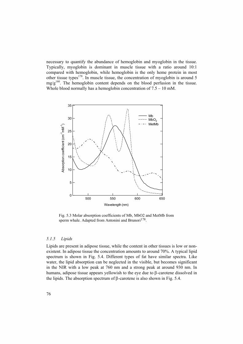
76
necessary to quantify the abundance of hemoglobin and myoglobin in the tissue.Typically, myoglobin is dominant in muscle tissue with a ratio around 10:1compared with hemoglobin, while hemoglobin is the only heme protein in mostother tissue types178. In muscle tissue, the concentration of myoglobin is around 5mg/g180. The hemoglobin content depends on the blood perfusion in the tissue.Whole blood normally has a hemoglobin concentration of 7.5 – 10 mM.
5.1.5 Lipidexistespectrwaterin thehumathe lip
35
30
25
20
15
10
5
0
Abs
orpt
ion
coef
ficie
nt (c
m-1
mM
-1)
650600550500
Wavelength (nm)
Mb MbO2 MetMb
Fig. 5.3 Molar absorption coefficients of Mb, MbO2 and MetMb fromsperm whale. Adapted from Antonini and Brunori178.
Lipidss are present in adipose tissue, while the content in other tissues is low or non-nt. In adipose tissue the concentration amounts to around 70%. A typical lipidum is shown in Fig. 5.4. Different types of fat have similar spectra. Like, the lipid absorption can be neglected in the visible, but becomes significant NIR with a low peak at 760 nm and a strong peak at around 930 nm. Inns, adipose tissue appears yellowish to the eye due to β-carotene dissolved inids. The absorption spectrum of β-carotene is also shown in Fig. 5.4.

5.1.6 Melaninorganelis insolMcAulihave pr
where λsharp fefilter wwhen pproblemhigh co
0.14
0.12
0.10
0.08
0.06
0.04
0.02
0.00
Lipi
d ab
sorp
tion
coef
ficie
nt (c
m-1
)
1000900800700600
Wavelength (nm)
β -carotene absorption coefficient (a.u.) Soy bean oil β-carotene
Fig. 5.4 Absorption coefficients of lipid and β-carotene. The β-carotenespectrum is not shown to scale. From Eker181.
77
Melanin is the dark pigment present in skin, hair, and the iris. It is synthesized by
les called melanosomes. Melanin cannot be refined in its pure form, since ituble, and the chemical structure becomes altered by extraction. Jacques andffe have investigated the absorption coefficient of the melanosomes182, andesented an approximate empirical formula183:
-148.312 cm 1070.1 −λ⋅=µ a (5.1)
is in nm. This spectrum is shown in Fig. 5.5. The spectrum presents noatures, and since the melanin is present only in a thin layer, it acts as a grayhen measurements through the skin are performed. This can be a problemerforming measurements on persons with very dark skin. Melanin is also a for optical detection of malignant melanoma, often containing melanin in
ncentration, since most of the light is then absorbed in the lesion.
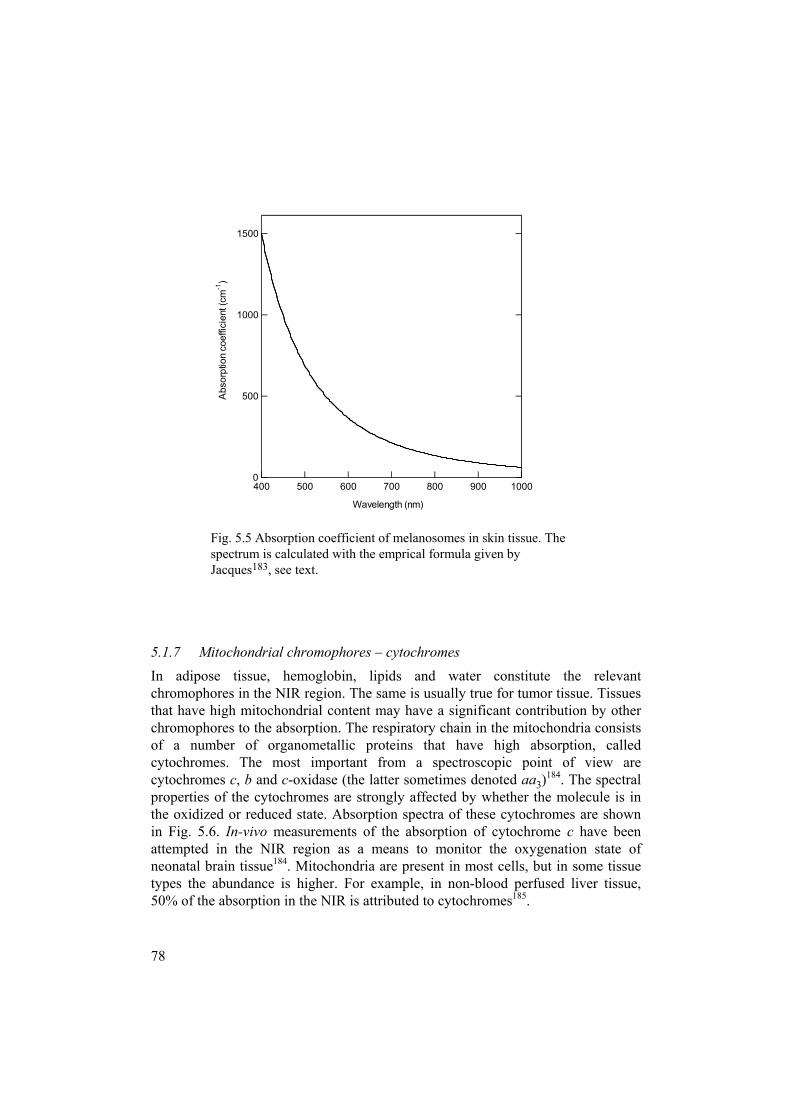
78
5.1.7 MIn adipochromopthat havechromopof a nucytochromcytochrompropertiethe oxidiin Fig. 5attemptedneonatal types the50% of th
1500
1000
500
0
Abs
orpt
ion
coef
ficie
nt (c
m-1
)
1000900800700600500400
Wavelength (nm)
Fig. 5.5 Absorption coefficient of melanosomes in skin tissue. Thespectrum is calculated with the emprical formula given byJacques183, see text.
itochondrial chromophores – cytochromesse tissue, hemoglobin, lipids and water constitute the relevant
hores in the NIR region. The same is usually true for tumor tissue. Tissues high mitochondrial content may have a significant contribution by otherhores to the absorption. The respiratory chain in the mitochondria consistsmber of organometallic proteins that have high absorption, called
es. The most important from a spectroscopic point of view arees c, b and c-oxidase (the latter sometimes denoted aa3)184. The spectral
s of the cytochromes are strongly affected by whether the molecule is inzed or reduced state. Absorption spectra of these cytochromes are shown.6. In-vivo measurements of the absorption of cytochrome c have been in the NIR region as a means to monitor the oxygenation state ofbrain tissue184. Mitochondria are present in most cells, but in some tissue abundance is higher. For example, in non-blood perfused liver tissue,e absorption in the NIR is attributed to cytochromes185.

5.1.8 The regof tissulower myoglomay, houtilizedfor tranphysiolanalysisbelievewith thfrom sp
0.01
0.1
1
10
100A
bsor
ptio
n co
effic
ient
(cm
-1m
M-1
)
1000900800700600500
Wavelength (nm)
Cyt aa3 (ox) Cyt aa3 (red) Cyt b (ox) Cyt b (red) Cyt c (ox) Cyt c (red)
Fig. 5.6 Molar absorption coefficients of cytochromes b, c and c-oxidase(aa3). From Cope184.
79
Discussion – absorption properties of tissueion approximately 650 – 1000 nm is sometimes called the optical windowe, due to the low overall absorption in this region. The scattering is alsoin this region compared with the UV and visible. Hemoglobin andbin are, in practice, indistinguishable in the region. The oxygen saturationwever, be determined by using in principle only two wavelengths. This is
in pulse oximetry186,187, and it is a major goal for most proposed modalitiessillumination. The oxygen saturation gives important information of theogy of the tissue, especially if it can be combined with imaging and/or of dynamic changes in oxygen saturation. For example, it is generally
d that the oxygen saturation differs markedly inside tumors as comparede surrounding tissue. Various methods to determine the oxygen saturationectral measurements have been presented in the literature105,106,131,188-198.

80
By adding more wavelengths to the analysis, it is possible to characterize moresubstances in the tissue. The aim of optical tomography of soft tissues is toquantify the concentrations of the four spectrally relevant chromophores in theoptical window: oxy- and deoxyhemoglobin, water, and lipids. To achieve this, inprinciple four wavelengths are needed, e.g., around 660 nm, 800 nm, 920 nm and970 nm. It is hoped that the information given by the state of oxygen saturation,together with the concentrations of water and lipids, the tissue morphology, andpossible dynamic changes, will provide enough information to diagnose diseasessuch as malignant lesions.
The distribution of chromophores on a small-scale level can be an important factorfor the overall absorption properties. The chromophores are, as we have seen, oftenconfined to discrete compartments on a cellular level. Also, the capillary networkof blood vessels is a highly inhomogeneous structure on a microscopic level. Whenchromophores are accumulated in certain regions, shielding effects occur, resultingin a reduced overall absorption. Since transport theory assumes homogeneousdistribution of absorbers on a microscopic level, the deduced absorption coefficienttends to be underestimated. Thus, the same volume concentration of, e.g.,hemoglobin in tissue results in different absorption depending on how thesubstance is distributed. This phenomenon has been studied by several authors, andcorrected transport models have also been developed106,199-202. As a somewhatsimplified explanation, this effect can also describe the increased absorptioncoefficient of flowing blood, as compared with non-flowing blood, reported inPaper V. In non-flowing blood, the red blood cells tend to form aggregates, andshielding effect thus occur. However, in whole blood, the scattering effects are toocomplicated for this description to be complete, as is discussed in more detail inPaper V.
5.1.9 Optical properties of bloodAt first glance, blood appears to have deceivingly simple optical properties. Thescattering and absorption are largely governed by the red blood cells (RBCs): theirrefractive index in relation to that of the surrounding plasma, and their absorptiondue to hemoglobin. The RBCs are virtually identical, biconcave discs with thedimensions approximately 2×8 µm. Unlike most other cells, they have no nucleus,so the scattering occurs only at the interface defined by the outer cell membrane. Ithas been shown that the scattering of the membrane itself is negligible203,204,meaning that only the size, shape and index mismatch are the relevant parameters.The refractive index of blood plasma has been measured to 1.345205, and therelative refractive index of the RBC to 1.04 – 1.05 at 633 nm206.

81
The complexity of blood optics comes from the fact that it is a moving liquid witha very dense concentration of RBCs. Many studies have concluded that the lighttransmission through flowing blood can change as much as 30% depending on theflow rate. When attempting quantitative optical measurements of blood, such alarge variation is not acceptable unless its mechanisms are understood and can becontrolled. The optical properties of blood in motion was investigated in Papers Vand VI. The key issue is understanding the microscopic geometry of the RBCs in aflow field, both in terms of deformation and their orientation, and how this relatesto the light scattering and absorption. Detailed studies of the behavior of RBCs inflowing blood were performed in the 1960s and 70s, and have revealed severalimportant observations about the morphology of the RBCs. Many experimentswere conducted on diluted blood, because of the easier experimental requirements.However, both the rheological and optical properties are very different for wholeblood, which has a volume density of about 40% RBCs.
To get reliable data for whole blood, different experimental techniques have beenused, e.g., snap freezing blood vessels with liquid nitrogen207, or microscopicphotography of thin layers of blood subjected to shear flow in viscometers208-212.The basic assumption made in the latter method is that it is the shearing in the flowfield that gives rise to changes in RBC morphology. For a liquid flowing through aduct, the shear rate is the velocity gradient perpendicular to the duct wall. In acircular duct, the velocity profile is parabolic for laminar flow of a Newtonianliquid (Poiseuille flow), and the shear rate varies linearly with the maximum valuesat the wall. Blood is generally considered a non-Newtonian liquid, however, andpropagates with a blunted parabolic profile, which becomes a flat “plug” if thediameter of the duct is small enough209,213,214. For ducts with a diameter larger than100 µm, the velocity profile is fairly well approximated with the parabolic. Theshear rate for a duct of circular cross section, with radius R, is given by
rRQG 2
4π
= (5.2)
where Q is the volumetric flow and r is the radial distance from the central axis.With this assumption of shear rate as the background, by studying the behavior ofRBCs in a viscometer one can emulate the shear rate in a duct at different radialdistances from the central axis.
Another method to study high concentrations of cells is by preparing ghost cells,which are index matched with the surrounding liquid. These become invisible inthe microscope, but retain their mechanical properties. By adding a small amountof tracer cells with the original optical properties, one can study the morphologyunder a microscope209. These methods have revealed that the RBCs behave muchlike liquid droplets dispersed in the blood plasma, rather than as rigid particles. At

high shear rate, the RBCs tend to elongate and align in the direction of the shear.At low or zero shear rate the situation is also complicated. The RBCs tend to formaggregates in various forms, e.g. the famous rouleaux, in ways that are governed bythe biochemistry of the cell membrane surfaces and the composition of the plasma.In Fig. 5.7, sketches of aggregated blood cells are depicted at various shear rates. Innormal human blood, almost all aggregates become dispersed at shear rates above46 s-1 208,210. However, even at higher shear rates, small roleaux of 4 – 10 cells mayresist and tumble along with the single cells. The aggregation properties of bloodare the reason for the nonlinear viscosity as the shear rate increases, and thus thefact that blood may be described as thixotropic, i.e., the viscosity is higher at lowshear rate. Aggregation also affects the scattering properties strongly, as was seenin Paper V.
The morphology of RBCs can also be studied using indirect methods such asmeasurements of the angular distribution of scattered light from thin layers –ektacytometry205. Several attempts to describe the scattering from individual RBCshave been made. By using T-matrix computations, it is possible to model theeffects of both deformation and orientation of single RBCs9. However, because theRBCs are so densely packed, single cell models fail to accurately predict the
Fig. 5.7 Sketches of RBCs. In (a), tracings of of deformation and orientation are shown at75 ms intervals. The direction of flow and time axis is downward in the picture; fourdifferent RBCs are shown. The shear rate was approximately 7 s-1. From Ref. 209. In (b),aggregation of RBCs in rouleau networks at low, increasing, shear rate are shown. Theshear rates are: A, 2.3 s-1; B, 23 s-1; C, 46 s-1; D, E, >46 s-1. From Ref. 208.
82

83
scattering of whole blood. In Paper V, it was demonstrated that qualitativepredictions of the scattering from whole blood are possible using T-matrix theory,and for the absorption one can almost draw quantitative conclusions.
A full understanding of the scattering properties of blood is of great importance.Such knowledge is a necessary requirement for in-vivo spectroscopicalmeasurements of anything else than oxygen saturation. Blood analysis is acornerstone of modern health care, and more efficient measurement methods wouldhave both benefits for the economy as well as for the patients and medical staff. Along-sought technique is non-invasive monitoring of blood glucose in diabetics,where optical sensors in one proposed method. Although in-vivo transilluminationmeasurements of blood may still be unrealistic for some time, hemodialysismachines are an area where the developments have lead to implementation ofoptical sensors.
5.2 Tissue phantomsArtificial samples are important for validation of light propagation models andsystems for measuring the optical properties, and in some cases also for calibration.The ideal phantom material should mimic the optical properties of tissue in termsof scattering coefficient, anisotropy factor, absorption coefficient and refractiveindex, over the entire spectral range of interest. It should also be possible to checkthe optical properties to high accuracy using independent methods, preferablybased on fundamental theory such as Mie calculations. Moreover, the materialshould be easy to make and shape, and be robust and stable.
In the field of tissue optics, most phantoms that have been used have been based oneither water or resins such as polyester. In the following two sections thesematerials will be discussed in more detail, to see how close they come to the idealphantom material.
5.2.1 Water-based phantomsPerhaps the simplest and most widely available phantom material is ordinarymilk215. The scattering in milk comes from fat droplets and proteins suspended inthe water. Absorption can be obtained by adding dyes or ink. In pure milkabsorption is dominated by the water, which has low absorption in the visiblespectrum but becomes increasingly large in the NIR. The relatively largeabsorption at 970 nm is a problem for water-based phantoms, since the absorptionof pure water can actually be higher than that of tissue, especially if the tissue is
84
low in water content such as fatty tissue or skin. Water phantoms are, for thisreason, not ideal for wavelengths above 900 nm.
Milk has obvious disadvantages as a phantom material, since its optical propertiesare not well defined and are not possible to verify by theory. Similar to milk interms of composition is Intralipid, which is perhaps the mostly used phantommaterial in the literature107,113,121,216-219. Intralipid is a nutrition liquid which isintended for intravenous use. The quality control is therefore much higher than formilk, and since it is sterile it can be kept longer. Addition of penicillin preventsbacterial growth. It should be noted, though, that it is not intended as an opticalproduct and the optical properties are still not particularly well defined. VanStaveren et al. gave approximate formulae for the scattering properties ofIntralipid-10%216:
lmlmm016.0 -1-14.2−λ=µ s (5.3)
λ−= 58.01.1g (5.4)
where the wavelength λ is in micrometers. Experience shows that the variation canbe in the order of 20% from the values predicted with this formula, possibly more.Liquid phantoms may be easy to work with, but make it difficult to introduceinhomogeneities. Solid Intralipid phantoms can be made by adding agar gel219.When adding an absorber, one has to be careful not to use one that changes thescattering properties. Generally, acidic dyes can cause the fat emulsion of theIntralipid to split. Food dyes are convenient to work with in the visible region, butthe region above 800 nm is more difficult. Carbon-based inks absorb in the NIR,but they also add some scattering, which makes absolute prediction of theabsorption difficult220.
The best water-based phantom is a suspension of monodisperse microspheres,usually of polystyrene. Since the size of the scattering spheres is known, it ispossible to use Mie theory of calculate the scattering properties. By choosing theright size, the g-factor can be controlled, something that is impossible withIntralipid. Unfortunately, monodisperse microspheres are expensive, and largevolume phantoms are not realistic. Microsphere suspensions keep longer thanIntralipid, but have a limited shelf life due to settling and aggregation of thespheres (in the order of months).
5.2.2 Resin phantomsFor realistic phantoms in the region above 900 nm, other materials than water arerequired. In addition to solving the absorption problem, plastics are attractive for

85
other reasons as well. Plastics are stable and robust, and solid phantoms make forthe possibility of complicated shapes and embedded inhomogeneities. Thedisadvantages are mainly the increased complexity in making them, and that it isnot possible to alter the properties of a phantom once it has set. Thermoplasticssuch as PMMA, although optically good, are not suitable because of thecomplicated production process. Curing plastics such as polyester and epoxy resinshave been used as phantom material, and are easy to work with in the laboratorysince the scattering and absorption agents can be mixed with the liquid resin.Polyester and epoxy have similar optical and mechanical properties221,222, but forlarge volumes (about 0.5 liter) epoxy is preferred since the heat from theexothermic process in the curing of the polyester can cause cracking.
As scatterers, the most common material is TiO2. This is an inexpensive andreadily available material, suitable where a tissue-like g-factor is not necessary orthe reduced scattering is the only important parameter. To control the g-factor,silica microspheres can be used as scatterers222, although at a considerably highercost. Many absorbing dyes are available in the visible region, but in the NIR thesituation is different. One dye, Pro Jet 900 NP, has proved compatible with bothpolyester and epoxy, and is effective up to around 900 nm222. Above 900 nm, thereis a small selection of commercially available laser and printing dyes223,224, but theexperience is that all of these tend to react with the resin and change theirabsorption properties, usually by almost complete bleaching. The simplest solutionto this problem is to use a broadband absorbing pigment such as carbon black,which is available everywhere in the form of toner for copying machines.
5.2.3 Refractive index
In phantoms with values of µs typical to tissues, the bulk material (water or resin)amounts to 99% or more. The refractive index is therefore close to 1.33 in waterphantoms and 1.55 in resin phantoms. For validation purposes, the difference inrefractive index compared with real tissue may not be of concern, since a modelthat is accurate for n = 1.33 or 1.55 is likely to be so for n = 1.4 (typical of tissues)as well. For calibration purposes this can be a matter that has to be taken intoconsideration, however, especially if time-resolved measurements are performed.
5.3 InstrumentationThe instrumentation needed to measure the optical properties of turbid mediadepends on the type of measurement. In this section, some of the most commontechniques are reviewed. The discussion follows the same structure as in Chapter 4,

86
The inverse problem. In general, the complexity of the instrumentation increasesgoing from cw measurement, over frequency-resolved measurements, to time-resolved measurements.
5.3.1 Cw measurement instrumentsSpatially resolved diffuse reflectance measurements (cf. Sect. 4.1.1) can beperformed in either contact mode or as image reflectometry. As light sources,either halogen lamps or Xe lamps are often employed, or light from LEDs or diodelasers. Broadband lamps require the use of some spectroscopic filtering at thedetection side, while diode lasers are intrinsically narrowband, but instead requirethe use of several units to cover many wavelengths. A diode-laser based, contactmode system was used in Paper II. The probe head in this case consists of a singlesource fiber in the center, and the detection is performed at different radialdistances by means of concentrically arranged rings of optical fiber bundles. Atechnical description of this system can be found in Ref. 102.
Examples of other fiber probe contact mode systems are those designed by Wilsonet al.225 and by Sterenborg and co-workers105, also intended for in-vivomeasurements on the skin. These systems utilize a white light source, and aspectrometer/CCD camera for detection.
In image reflectometry, the surface is illuminated at one point, and a camerarecords the diffuse reflectance pattern around the light spot. Such a system isdescribed in Ref. 107, where an imaging Fourier-transform interferometer was usedto provide both imaging and spectral resolution. One possible advantage of imagereflectometry over contact mode systems is that the surface is left undisturbed,which can be a problem for skin measurements because the blood flow is restrictedby the pressure applied by the probe head. The drawback of image reflectometry isthat it may be more difficult to keep the object still in relation to the instrumentduring the acquisition. To make image reflectometry more robust with respect tosmall inhomogeneities, it is also possible to illuminate the surface with a structuredpattern instead of at a single point. The data evaluation then requires someadditional processing which typically involves Fourier transformation of the imageof the reflected pattern226.
The general advantage of cw measurements is the simplicity and robustness of theinstrumentation. The technique has some drawbacks as compared with frequency-or time-resolved measurements, as was discussed in Sect. 4.1.2. A thoroughtreatment on cw measurements can be found in Ref. 129.
87
5.3.2 Frequency-resolved instrumentsFrequency-modulated diode lasers are the usual choice of light source forfrequency-resolved instruments. The modulation is performed at radio frequenciesup to around 1 GHz. Avalanche photodiodes are typically used as detectors. Thelight is most often delivered to the medium by means of a multimode optical fiber,and the detected light is guided to the detector by a similar fiber or a fiber bundle.Thanks to the inherent homodyne detection implemented by this scheme,frequency-resolved measurements can yield very low-noise signals. The low-noisedata is advantage compared with time-resolved measurements, but on the otherhand, the information content is lower unless the measurements are performed atmany modulation frequencies. The maximum bandwidth is also usually lower for afrequency-resolved system than a time-resolved, which is important especially ifthe source and detector fibers are close. Close fiber spacing usually means <1 cmin biological tissues. A comparison between time-resolved and frequency-resolvedsystems can be found in Ref. 227. Frequency-resolved instruments for tissue opticsmeasurements have been built by several groups229-234.
5.3.3 Time-resolved instrumentsTime-resolved measurements of turbid media were pioneered in the middle 1980s,and first utilized mode-locked Ar-ion lasers and dye lasers that producedpicosecond pulses as light sources235,236. Since then, a multitude of pulsed lasershave been used, e.g., mode-locked Ti:sapphire lasers237, fiber lasers238, and diodelasers136,141,142. The requirement on the pulse length depends on the application, butfor tissue, at short source-detector distances, better than 100 ps (corresponding to10 GHz bandwidth) is usually necessary. At longer distances, approximately >2cm, pulse lengths of up to 0.5 – 1 ns can be tolerated. The requirement is that thewidth of the temporal point-spread function (TPSF) is larger than the width of theinjected pulses. (Here, the TPSF denotes the impulse response function of themedium. Often, the term TPSF is used for the actual measured curve, which hererepresents the TPSF convolved with the instrument response function).
The instrument response function is determined by the laser pulse length, and thebroadening in the instrument: mode dispersion in optical fibers, broadening in thedetector, time resolution and jitter in the electronics, etc. If long fibers are used,approximately > 1 m, they should be of gradient index type to eliminate pulsebroadening by mode dispersion. Time-resolved detection can be achieved in anumber of ways. The most common detector is probably a high-bandwidthphotomultiplier tube (PMT). These can have impulse response times down to about0.5 ns. With direct sampling electronics or boxcar integrators, time-resolution ofthis order can be achieved. Kerr shutters have also been employed, but suffer from

poor dynamic range239. The most common technique, however, is time-correlatedsingle-photon counting (TCSPC). This method, illustrated in Fig. 5.8, is based onsingle photon statistics. The TCSPC method works at very low intensity levels,where individual photons are detected. It has advantages in terms of increased timeresolution, dynamic range, and sensitivity.
When a pulse from the detector arrives, corresponding to one detected photon, thisserves as a trigger pulse for the time-to-amplitude converter. When the pulsetriggers the converter, an internal clock is started. The clock stops when thephotodiode gives an electric pulse directly from the input light pulses, or acorresponding synchronizing signal from the laser driver. The time difference isconverted to an electric pulse with an amplitude that is directly proportional to thetime difference. This pulse is fed to a multichannel analyzer which converts thepulse amplitude to a channel number, which is then stored in a computer memory.The process is repeated, and each time a photon is detected it will add one count toone of the channels. Eventually, a histogram representing the shape in time of thesignal forms. The probability of two or more photons reaching the detector at thesame time must be low, since a second photon from the same laser pulse will notbe counted. This would skew the distribution towards early times, the so-calledpile-up effect. If the probability of detecting one photon per laser shot is keptbelow 1:30, the pile-up effect becomes negligible240.
Sample
PMT
Photodiode
Start signalfrom detectedphoton
Stop signalfrom laser pulse
Clock∆t
∆t
∆VTAC
N counts
Channel
∆V
Standard pulse
MCACFD
CFD
Fig. 5.8 The principle of time-correlated single-photon counting. Abbreviations used inthe figure: PMT- photomultiplier tube, CFD – constant fraction discriminator, TAC –time-to-amplitude converter, MCA – multichannel analyzer. See the text for anexplanation.
88

89
A typical mode-locked Ti:sapphire laser or pulsed diode laser may have arepetition rate of 80 MHz, so the count rate can easily exceed 1 MHz and thesystem is still in the single-photon counting mode. Since the measurement isreduced to binary mode (photon or no photon), the dynamic range of the detector isnot an issue. In the same way, it is only necessary to know when in time the pulsesarrive, which renders the shape of the pulses largely irrelevant. A constant fractiondiscriminator is used to accurately determine the arrival times of the pulses,independently of their amplitude, and the temporal resolution of the measurementcan be 1/10 that of the rise time of the detector, or a few tens of picoseconds.
To be able to keep count rates as high as 1 MHz or above, the dead time of thedetection system is an important parameter. The dead time for a PMT is largelydetermined by the transit time of the electrons. To minimize the transit time,special PMTs are often used which are equipped with a microchannel plate toshorten the distances the electrons have to travel inside the detector.
The sensitivity of the TCSPC method is limited mainly by the dark count rate ofthe detector. If the limit is defined as an signal-to-noise (SN) ratio of 1, thesensitivity can be written as
TNR
QS cd1
= (5.5)
where Rd is the dark count rate, Nc is the number of time channels, T is the overallmeasurement time, and Q is the quantum efficiency of the detector241. The detectoris often cooled to reduce the dark count rate and thus obtain a better sensitivity.The accuracy of the measurement is directly determined by the counting statistics,where the noise per time channel is given by the usual expression N1/2 for N counts.Since it is usually important to keep the acquisition time to a minimum, the SNratio is often worse than for frequency-resolved measurements. Instruments basedon the TCSPC technique have been developed by several groups136,141,238, and wasalso used in Papers II and III.
Detection in the NIR region is a problem for TCSPC measurements, at least above900 nm. Standard multialkali photocathodes have good sensitivity up to ~800 nm,but it drops off rapidly at longer wavelengths242. Ag-O-Cs (S-1) cathodes areavailable, which are sensitive up to 1200 nm, but their sensitivity is, at best, anorder of magnitude lower at shorter wavelengths. The latest InP/InGaAs cathodesexpand the sensitivity out to 1700 nm, but the detector requires liquid nitrogencooling, have a short life span, and is also considerably more expensive242. Theregion 900 – 1000 nm is interesting in tissue optics because of the potential ofmeasuring lipid and water content in the tissue (cf. Sect. 5.1.8). At present, GaAs

90
cathode detectors sensitive in this region are available, but the instrument responsefunction of a TCSPC system with such a detector is not better than in the order of0.5 ns141.
Avalanche photodiodes are another option, but they too have a poor timeresolution. The region above 1000 nm is virtually unexplored with time-resolvedmeasurements, and is an interesting object for future research. An interestingpotential detector type for TCSPC systems are the emerging superconductingdetectors243,244. This detector type is based on a superconducting material, whichheats up slightly upon absorbing photons, and momentarily induces a detectableelectrical resistance. These detectors function at NIR wavelengths, have a highbandwidth, and negligible dark counts, i.e., TCSPC measurements with virtuallyunlimited sensitivity would be possible. The superconducting detectors are,however, at present too small (10×10 µm) to be practical for TCSPC instruments.
Another option to reach very good time-resolution is the streak camera240,245,246.Time-resolution better than 1 ps can be achieved, but the dynamic range of thestreak camera is not as good as for TCSPC systems. Streak cameras are oftencombined with spectrometers, and by using white-light pulses spectroscopicinformation can be obtained246.
Gated CCD cameras have also been used to obtain a time-resolved detectionsystem, and have the advantage of yielding parallel measurements. The time-resolution is not great, however, in the order of 0.5 ns247.
5.3.4 Optical tomography instrumentsInstruments for optical tomography are essentially parallel, or scanning, versions ofone of the instrument types described in the previous sections. The practicaldifficulties of constructing such a system can be great, and the number of freeparameters is large. The design must be a compromise between engineeringconsiderations, patient comfort, and the optimal measurement in terms ofreconstruction. An early optical tomograph, based on cw measurements andintended for optical mammography (breast cancer detection, cf. Sect. 5.4), wasbuilt at Philips248. Other cw systems have been built more recently249,250, and havethe advantage of being relatively simple, and that large quantities of data can beacquired in short time. The drawback of cw systems is that image reconstruction ishampered by the limited information in the intensity measurement (cf. Sect. 4.5).
Frequency-resolved optical tomography was initiated by Gratton et al.251. An earlycommercial attempt of a scanning, frequency-resolved optical mammographysystem was built at Carl Zeiss252,253. A contemporary instrument was designed at

91
Siemens, but details and results have not been widely published. Both companieshave now abandoned development in the area. Other systems have later been builtby several groups230-234, and designs for new generation systems are presently beingpursued by many groups, primarily in the United States. Some of these systems arecombined cw/frequency-resolved instruments. Bevilaqua et al. used a white cwlight source to provide additional spectral information230. Another advantage of thecombined instrument is that dynamic changes can be monitored thanks to the shortacquisition time and simple reconstruction of cw data, while the frequency-resolved data yields information of the absolute optical properties231.
Time-resolved scanning mammographs, intended for transillumination of breasts,have been built for clinical use136,141,254. Currently, these systems are not used fortrue reconstruction of the optical properties, but the measurement protocol could inprinciple be modified to accommodate a wider range of projections which wouldallow tomographic reconstruction. A time-resolved 32-channel optical tomographysystem has been constructed by the group of Delpy238, and has been used formonitoring of oxygen saturation in neonatal brain255, the forearm154, opticalmammography for detection of breast cancer256, and extensive phantomstudies151,152,155,257. Another fully tomographic system, allowing parallel detection ineight channels, has been built by Chance and collaborators258,259.
5.4 Optical mammography – a diagnostic applicationEarly on, breast cancer detection was identified as one of the most promising goalsof optical tomography in medicine142. The female breast is easily accessed for atomography system, and although the tissue structure is by no meanshomogeneous, it is still more homogeneous than many other organs. A majormotivation for optical mammography is that current diagnostic modalities are lessthan perfect in many respects. Conventional x-ray mammography suffers frompoor contrast, and physicians are forced to look for subtle morphological variationor secondary effects such as microcalcification. The efficacy of screening programshas been debated, and there is also a real statistical risk of inducing cancer in asmall number of cases due to the ionizing nature of x-rays. Sonographicexaminations have been proposed, but have so far emerged rather as a complementto x-rays than as an alternative. Magnetic resonance imaging is a perfect methodfor structural imaging, but without injected contrast agents to provide functionalinformation it has proved difficult to distinguish malignant and benign lesions. It isalso a costly technique.
Simple schemes for transillumination of the breast using lamps and photographicfilm or video cameras have been tried since the 1920s, but all these attempts

92
proved to be inferior to conventional x-ray mammography260. In terms ofresolution, optical mammography can never hope to compete with x-rays. Itexpected that the best obtainable resolution for deep tissue structures is in the orderof 0.5 – 1 cm. The advantage is instead hoped to be better contrast, and the abilityto provide functional imaging, e.g., a different oxygen saturation in malignantlesions can serve as a distinct marker.
Many of the optical tomography systems described in the previous section weredesigned with optical mammography as a primary objective136,141,231,233,248,251,253,254.In addition to technical developments, an important area of research isunderstanding the scattering and absorption properties of various tissue types, andhow these are linked to physiological parameters influenced by for example ageand hormonal cycle. Clinical trials are ongoing in both Europe and the UnitedStates141,231,256,261-267. One company specializing in development of opticalmammography is active in Fort Lauderdale, Florida268, but their results have notbeen widely published in the scientific literature.
5.5 Atmospheric optics – remote sensing of trace gasesThe primary application of spectroscopic techniques in atmospheric optics isremote sensing of trace gases in the atmosphere. Remote sensing techniques can beeither passive, utilizing the natural light directly or indirectly from the sun, oractive, utilizing for example lasers as light sources. Passive techniques areattractive because of the simplicity of the instrumentation, but having control of thenatural light source can be problematic. Among the important trace gases from aremote sensing perspective we find SO2, NO2, O3, and numerous hydrocarbons.Hydrocarbons have strong characteristic absorption bands in the infrared, wherethe scattering in the atmosphere usually is negligible. Spectroscopy of the othergases, however, is performed at shorter wavelengths, in the visible region for NO2,and UV for SO2 and O3. In this region, both the Rayleigh scattering from the airand scattering from dispersed aerosols can be significant.
In Paper VII, both passive and active techniques were applied to measure theemission of SO2 from the volcano Mt. Etna in Italy. The passive instruments werea differential absorption spectroscopy (DOAS) system240,269, and a correlationspectroscopy (COSPEC) instrument240,270. A lidar system (light detection andranging) was used to provide active measurements, using a pulsed dye laser as thelight source. A differential absorption lidar (DIAL) measurement scheme wasapplied, in which the absorption on and off one absorption peak of the gas ismeasured240,271. Passive systems can operate in either up-looking or sun-trackingmode. In the former mode, the light is provided by the blue sky above the

93
instrument, and the trace gas is assumed to linger between the detector and thescattering volume in the atmosphere. In the latter mode, the sun disc directlyprovides the light. Passive instruments usually have to be calibrated for eachmeasurement, due to the variation in solar elevation, background absorption, cloudformation etc.
The passive instruments operate at around 300 nm, where the atmosphericscattering is strong enough to disqualify the assumption of a clear medium betweenthe light source and the detector, especially in the up-looking mode. This mode ispreferred because of the simplicity. The path-length of the detected light throughthe gas is then no longer trivial to predict. If a line-of-sight path-length is assumed(the Beer-Lambert law), the measured gas concentration will be systematicallyoffset; usually it is overestimated due to a longer actual path-length in thescattering medium.
The scattering in the atmosphere can be divided in two parts, Rayleigh-typescattering from the air molecules and Mie-type scattering from aerosols. TheRayleigh contribution is determined by the well-known expression for the scatteredenergy I:
20
24
4
316 Eα
λπ
=cI , (5.6)
where α is the polarizability of the molecule and E0 is the amplitude of the electricfield. The real atmosphere deviates slightly from this theoretical formula. Anempirical formula for the Rayleigh cross section in the region 200 – 550 nm wasgiven by Nicolet272:
2432 m 1002.4 xR
+− λ⋅=σ
3228.00.09426389.0 −λ
+λ=x , (5.7)
where λ is expressed in µm. To obtain the scattering coefficient, the numberdensity of air molecules is needed. This depends on the air density which is afunction of air pressure and the altitude. One can assume that it follows thestandard atmosphere model273. This calculation was performed to obtain thescattering coefficients in Paper VII.
The contribution of aerosols to the scattering is high in the lowest layers of thetroposphere. The exact composition of the aerosol layer varies strongly dependingon climate zone, weather conditions, the ground conditions, and is alsosignificantly influenced by anthropogenic factors in densely populated areas. The

94
measurements in Paper VII were carried out at sea, where the aerosol layer mostlyconsists of water droplets relatively close to the sea surface, usually with a radius< 1 µm. If the composition of particles is known, it is possible to calculate thescattering coefficient by means of Mie theory. However, because the aerosols werenot sampled and characterized during the measurements, the scattering was insteadestimated with the formula
1-km 55.0
)550(912.3 qRss V
λ
⋅
µ−=µ
3/1585.0 Vq = , (5.8)
where V is the observed visibility [km], µsR(550) is the Rayleigh scattering
coefficient at 550 nm [km-1], and the wavelength λ is expressed in µm274. Theobserved visibility is hardly an exact quantity, so the scattering coefficientcalculated by Eq. (5.8) is a very approximate estimate. However, the modeldeveloped in Paper VII turned out to be fairly insensitive to variations in thescattering coefficient at lower altitudes, so the approximations seem warranted.
The Monte Carlo model applied in Paper VII was based on reciprocal computationof the detected light (cf. Sect. 3.2.4; Reciprocity). Since the passive instrumentswere essentially point detectors with a narrow angle of collection, thecomputational photon economy was improved enormously by launching thephotons at the detector and tracing them backwards. By recording the path-lengththrough the volcanic plume, it was possible to derive correction factors for thesystematic effects of the passive instruments. Considering the approximationsmade in the model, the corrections agreed well with measurements of the SO2concentration performed with the active lidar system.
Systematic effects due to scattering in passive instrument readings have beenmodeled previously by Millán for low-altitude gas plumes275. The Monte Carlomodel presented in Paper VII extends those results to more general conditions.Emission of SO2 has important environmental implications, and is a major sourceof acidic rain. It is also believed that SO2 can be converted to sulfate aerosols,which can have an impact on cloud formation, and thus in the long run, on theclimatic systems276. Volcanic and anthropogenic emissions are two major sourcesof SO2. Routine monitoring of SO2 emissions must be performed using therelatively simple, inexpensive and robust passive instruments, and it is thusimportant to be able to quantify the systematic effects due to scattering in thereadings.

95
Acknowledgements
I am grateful for all the help and support from a large number of people, includingcolleagues and staff at the Atomic Physics division, and all our collaborators atother institutions. Working with physics and technology, so closely related to directapplications in medicine and health care, has been truly inspiring.
Först av allt vill jag tacka min handledare Stefan Andersson-Engels för hansvetenskapliga ledarskap, och även som en god vän på jobbet, på alla våra resorvärlden över till olika konferenser och möten, och inte minst olika aktiviteterutanför jobbet. Att välta med racekanoten på Ringsjön varje år har blivit något aven klassiker... Jag är också mycket tacksam för samarbetet med min ”vice”handledare Sune Svanberg, som var den som fick mig att börja påAtomfysikavdelningen tack vare hans kombination av pedagogisk förmåga,entusiasm och förmåga att kunna inspirera sina medarbetare. Flera andra senioraforskare, post-docs, administrativ personal och doktorander har också bidragit tillden fina atmosfären på avdelningen. Jag vill särskilt tacka tidigare och nuvarandemedlemmar av medicingruppen. Några har stått särskilt nära mig, och jag vill tackaThomas Johansson för att han har hållit sin halva av vårt arbetsrum likaoorganiserad som jag har hållit min. Sara Pålsson, Marcelo Soto Thompson,Christoffer Abrahamsson och Petter Weibring för fin vänskap och samarbete. Jagvill också tacka Annika Enejder – som jag står i tacksamhetsskuld till för att honhar dragit igång mycket av arbetet den här avhandlingen bygger på – Claes afKlinteberg, Jan Sørensen Dam och Ulf Gustafsson.
I also wish to thank the people involved in the Optimamm project. In particular,I’ve always felt welcome at the research group of Rinaldo Cubeddo at Politecnicodi Milano. A special thank you to Antonio Pifferi for our nice collaboration.
Ett stort varmt tack till alla mina vänner, och särskilt grabbarna på BK Smittansmejlinglista.
Jag är särskilt tacksam för allt stöd från mina föräldrar och familj under de häråren.
Till sist vill jag tacka Anette, för att du har stått ut med mig, och för att du är denunderbaraste i världen.

96
Summary of papers
Paper I New computational methods for prediction of fluorescence signals inlayered turbid structures, based on Monte Carlo simulations, weredeveloped and tested. The problem was divided in two parts: onecomputation for the excitation light, and one for the emittedfluorescence light. These two computations could then be convolvedto provide the solution. The computation time could be reduced by upto two orders of magnitude by reversing the photon trajectories whencomputing the emitted light. The theoretical foundation for thisprocedure, based on the reciprocity theorem in transport theory, wasalso treated.
Paper II-III In these papers, various systems for diffuse-reflectance measurementsof turbid media were used to determine the optical properties. In paperII, systems based on spatially resolved cw measurements, time-resolved measurements, and an integrating sphere, were comparedwith the help of phantom measurements. In paper III, two time-resolved systems were first characterized using phantommeasurements, and then used to measure the optical properties ofbreast tissue.
Paper IV The integrating sphere technique was used to measure the opticalproperties of myocardium that had been subjected to radio-frequencyablation therapy. The results could aid the development of an opticalprobe to guide such therapy in real-time.
Paper V-VI The integrating sphere technique was used to measure the opticalproperties of whole blood flowing through an optical cuvette. Theresults were compared with T-matrix computations of the scatteringfrom single red blood cells, and then discussed in terms of the effectsof changes in the cell shapes, orientation, and aggregation. In paperVI, polarized light was used to yield additional information. The limitsof singe-scattering theory for the case of whole blood were alsoexplored.
Paper VII A Monte Carlo model was developed to simulate light propagation inthe atmosphere and through a volcanic plume. The model couldsuccessfully explain systematic errors in the readings of passiveremote sensing instruments used to measure sulfur dioxide emissions,which arise due to light scattering. Reversed photon trajectories basedon the reciprocity principle were employed to accelerate thecomputations.

97
Contribution by the author to the papers
Paper I Substantial part of theoretical development, model coding, performingand evaluating simulations, and manuscript preparation.
Paper II Major part of integrating sphere measurements and evaluation,phantom preparation, and manuscript preparation. Substantial part ofspatially resolved and time-resolved measurements. Contribution toevaluation of spatially resolved and time-resolved data.
Paper III Substantial part of construction of the diode-laser based system andmeasurements using this system, and manuscript preparation.Contribution to evaluation.
Paper IV Contribution to in-vivo experiments. Major part of integrating spheremeasurement and evaluation. Substantial part of manuscriptpreparation.
Paper V Substantial part of experiments, evaluation and manuscript prepa-ration.
Paper VI Substantial part of experiments, evaluation and manuscript prepa-ration.
Paper VII Major part of Monte Carlo model and simulations. Substantial part ofmanuscript preparation. Contribution to evaluation.

98
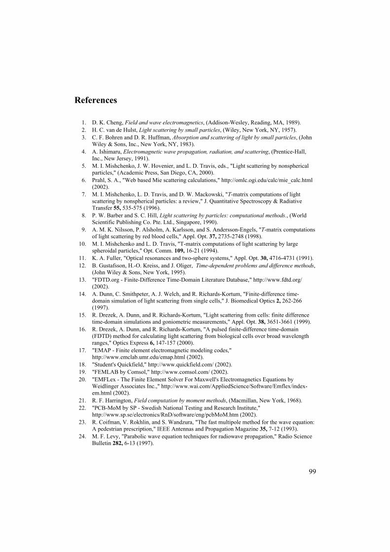
99
References
1. D. K. Cheng, Field and wave electromagnetics, (Addison-Wesley, Reading, MA, 1989).2. H. C. van de Hulst, Light scattering by small particles, (Wiley, New York, NY, 1957).3. C. F. Bohren and D. R. Huffman, Absorption and scattering of light by small particles, (John
Wiley & Sons, Inc., New York, NY, 1983).4. A. Ishimaru, Electromagnetic wave propagation, radiation, and scattering, (Prentice-Hall,
Inc., New Jersey, 1991).5. M. I. Mishchenko, J. W. Hovenier, and L. D. Travis, eds., "Light scattering by nonspherical
particles," (Academic Press, San Diego, CA, 2000).6. Prahl, S. A., "Web based Mie scattering calculations," http://omlc.ogi.edu/calc/mie_calc.html
(2002).7. M. I. Mishchenko, L. D. Travis, and D. W. Mackowski, "T-matrix computations of light
scattering by nonspherical particles: a review," J. Quantitative Spectroscopy & RadiativeTransfer 55, 535-575 (1996).
8. P. W. Barber and S. C. Hill, Light scattering by particles: computational methods., (WorldScientific Publishing Co. Pte. Ltd., Singapore, 1990).
9. A. M. K. Nilsson, P. Alsholm, A. Karlsson, and S. Andersson-Engels, "T-matrix computationsof light scattering by red blood cells," Appl. Opt. 37, 2735-2748 (1998).
10. M. I. Mishchenko and L. D. Travis, "T-matrix computations of light scattering by largespheroidal particles," Opt. Comm. 109, 16-21 (1994).
11. K. A. Fuller, "Optical resonances and two-sphere systems," Appl. Opt. 30, 4716-4731 (1991).12. B. Gustafsson, H.-O. Kreiss, and J. Oliger, Time-dependent problems and difference methods,
(John Wiley & Sons, New York, 1995).13. "FDTD.org - Finite-Difference Time-Domain Literature Database," http://www.fdtd.org/
(2002).14. A. Dunn, C. Smithpeter, A. J. Welch, and R. Richards-Kortum, "Finite-difference time-
domain simulation of light scattering from single cells," J. Biomedical Optics 2, 262-266(1997).
15. R. Drezek, A. Dunn, and R. Richards-Kortum, "Light scattering from cells: finite differencetime-domain simulations and goniometric measurements," Appl. Opt. 38, 3651-3661 (1999).
16. R. Drezek, A. Dunn, and R. Richards-Kortum, "A pulsed finite-difference time-domain(FDTD) method for calculating light scattering from biological cells over broad wavelengthranges," Optics Express 6, 147-157 (2000).
17. "EMAP - Finite element electromagnetic modeling codes,"http://www.emclab.umr.edu/emap.html (2002).
18. "Student's Quickfield," http://www.quickfield.com/ (2002).19. "FEMLAB by Comsol," http://www.comsol.com/ (2002).20. "EMFLex - The Finite Element Solver For Maxwell's Electromagnetics Equations by
Weidlinger Associates Inc.," http://www.wai.com/AppliedScience/Software/Emflex/index-em.html (2002).
21. R. F. Harrington, Field computation by moment methods, (Macmillan, New York, 1968).22. "PCB-MoM by SP - Swedish National Testing and Research Institute,"
http://www.sp.se/electronics/RnD/software/eng/pcbMoM.htm (2002).23. R. Coifman, V. Rokhlin, and S. Wandzura, "The fast multipole method for the wave equation:
A pedestrian prescription," IEEE Antennas and Propagation Magazine 35, 7-12 (1993).24. M. F. Levy, "Parabolic wave equation techniques for radiowave propagation," Radio Science
Bulletin 282, 6-13 (1997).
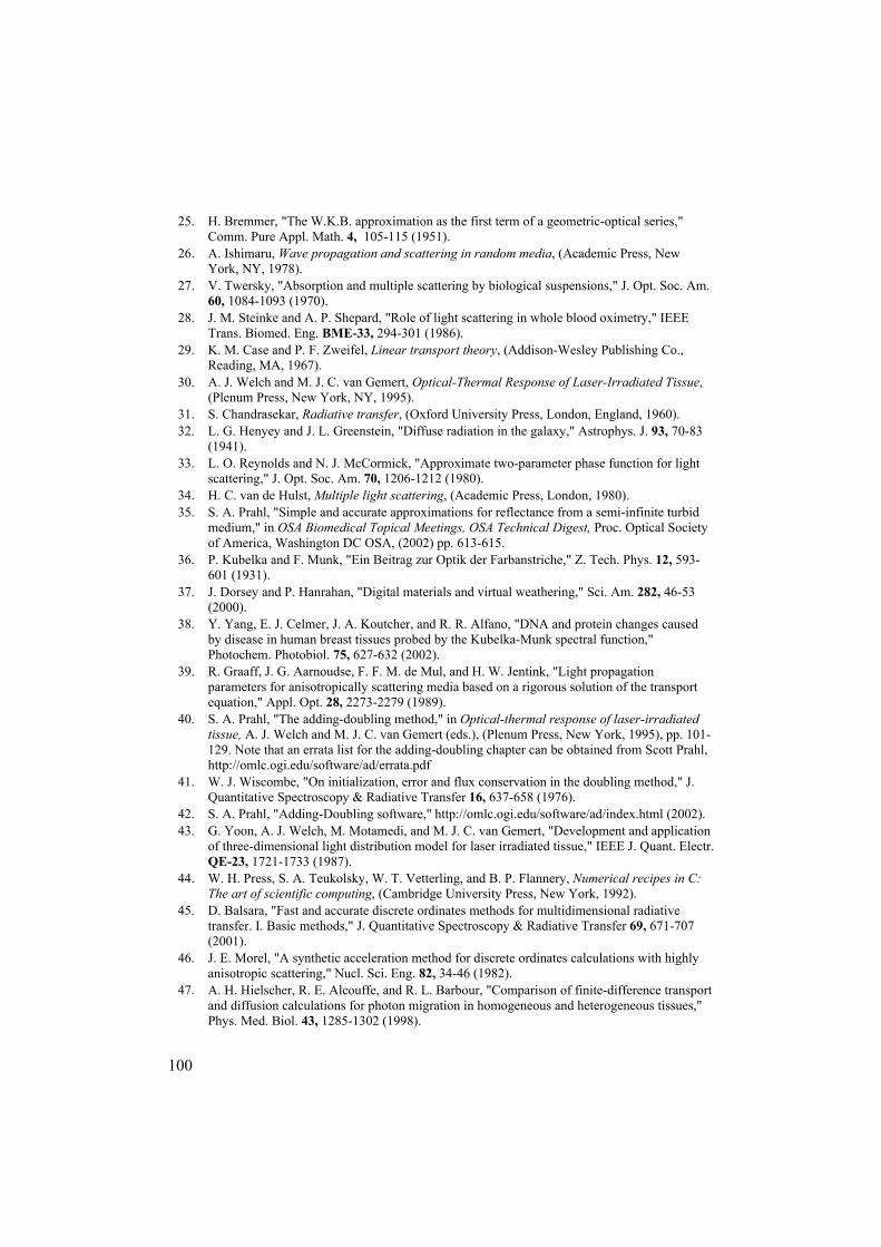
100
25. H. Bremmer, "The W.K.B. approximation as the first term of a geometric-optical series,"Comm. Pure Appl. Math. 4, 105-115 (1951).
26. A. Ishimaru, Wave propagation and scattering in random media, (Academic Press, NewYork, NY, 1978).
27. V. Twersky, "Absorption and multiple scattering by biological suspensions," J. Opt. Soc. Am.60, 1084-1093 (1970).
28. J. M. Steinke and A. P. Shepard, "Role of light scattering in whole blood oximetry," IEEETrans. Biomed. Eng. BME-33, 294-301 (1986).
29. K. M. Case and P. F. Zweifel, Linear transport theory, (Addison-Wesley Publishing Co.,Reading, MA, 1967).
30. A. J. Welch and M. J. C. van Gemert, Optical-Thermal Response of Laser-Irradiated Tissue,(Plenum Press, New York, NY, 1995).
31. S. Chandrasekar, Radiative transfer, (Oxford University Press, London, England, 1960).32. L. G. Henyey and J. L. Greenstein, "Diffuse radiation in the galaxy," Astrophys. J. 93, 70-83
(1941).33. L. O. Reynolds and N. J. McCormick, "Approximate two-parameter phase function for light
scattering," J. Opt. Soc. Am. 70, 1206-1212 (1980).34. H. C. van de Hulst, Multiple light scattering, (Academic Press, London, 1980).35. S. A. Prahl, "Simple and accurate approximations for reflectance from a semi-infinite turbid
medium," in OSA Biomedical Topical Meetings, OSA Technical Digest, Proc. Optical Societyof America, Washington DC OSA, (2002) pp. 613-615.
36. P. Kubelka and F. Munk, "Ein Beitrag zur Optik der Farbanstriche," Z. Tech. Phys. 12, 593-601 (1931).
37. J. Dorsey and P. Hanrahan, "Digital materials and virtual weathering," Sci. Am. 282, 46-53(2000).
38. Y. Yang, E. J. Celmer, J. A. Koutcher, and R. R. Alfano, "DNA and protein changes causedby disease in human breast tissues probed by the Kubelka-Munk spectral function,"Photochem. Photobiol. 75, 627-632 (2002).
39. R. Graaff, J. G. Aarnoudse, F. F. M. de Mul, and H. W. Jentink, "Light propagationparameters for anisotropically scattering media based on a rigorous solution of the transportequation," Appl. Opt. 28, 2273-2279 (1989).
40. S. A. Prahl, "The adding-doubling method," in Optical-thermal response of laser-irradiatedtissue, A. J. Welch and M. J. C. van Gemert (eds.), (Plenum Press, New York, 1995), pp. 101-129. Note that an errata list for the adding-doubling chapter can be obtained from Scott Prahl,http://omlc.ogi.edu/software/ad/errata.pdf
41. W. J. Wiscombe, "On initialization, error and flux conservation in the doubling method," J.Quantitative Spectroscopy & Radiative Transfer 16, 637-658 (1976).
42. S. A. Prahl, "Adding-Doubling software," http://omlc.ogi.edu/software/ad/index.html (2002).43. G. Yoon, A. J. Welch, M. Motamedi, and M. J. C. van Gemert, "Development and application
of three-dimensional light distribution model for laser irradiated tissue," IEEE J. Quant. Electr.QE-23, 1721-1733 (1987).
44. W. H. Press, S. A. Teukolsky, W. T. Vetterling, and B. P. Flannery, Numerical recipes in C:The art of scientific computing, (Cambridge University Press, New York, 1992).
45. D. Balsara, "Fast and accurate discrete ordinates methods for multidimensional radiativetransfer. I. Basic methods," J. Quantitative Spectroscopy & Radiative Transfer 69, 671-707(2001).
46. J. E. Morel, "A synthetic acceleration method for discrete ordinates calculations with highlyanisotropic scattering," Nucl. Sci. Eng. 82, 34-46 (1982).
47. A. H. Hielscher, R. E. Alcouffe, and R. L. Barbour, "Comparison of finite-difference transportand diffusion calculations for photon migration in homogeneous and heterogeneous tissues,"Phys. Med. Biol. 43, 1285-1302 (1998).

101
48. A. D. Klose and A. H. Hielscher, "Iterative reconstruction scheme for optical tomographybased on the equation of radiative transfer," Med. Phys. 26, 1698-1707 (1999).
49. A. D. Klose, U. Netz, K. Beuthan, and A. H. Hielscher, "Optical tomography using the time-independent equation of radiative transfer. 1. Forward model," J. Quantitative Spectroscopy &Radiative Transfer 72, 691-713 (2002).
50. S. R. Arridge, "Optical tomography in medical imaging," Inverse Problems 15, R41-R93(1999).
51. Y. Yamada, "Diffusion coefficient in the photon diffusion equation," in Optical Tomography,Photon Migration, and Spectroscopy of Tissue and Model Media: Theory, Human Studies,and Instrumentation, B. Chance, R. R. Alfano, and A. Katzir (eds.), Proc. SPIE 2389, (SPIE,1995), pp. 87-97.
52. T. Durduran, A. G. Yodh, B. Chance, and D. A. Boas, "Does the photon-diffusion coefficientdepend on absorption?," J. Opt. Soc. Am. A 14, 3358-3365 (1997).
53. T. J. Farrell, M. S. Patterson, and B. Wilson, "A diffusion theory model of spatially resolved,steady-state diffuse reflectance for noninvasive determination of tissue optical properties invivo," Med. Phys. 19, 879-888 (1992).
54. R. C. Haskell, L. O. Svaasand, T.-T. Tsay, T.-C. Feng, M. S. McAdams, and B. J. Tromberg,"Boundary conditions for the diffusion equation in radiative transfer," J. Opt. Soc. Am. A 11,2727-2741 (1994).
55. M. S. Patterson, B. Chance, and B. C. Wilson, "Time resolved reflectance and transmittancefor the non-invasive measurement of optical properties," Appl. Opt. 28, 2331-2336 (1989).
56. A. Kienle and M. S. Patterson, "Improved solutions of the steady-state and the time-resolveddiffusion equations for reflectance from a semi-infinite turbid medium," J. Opt. Soc. Am. A14, 246-254 (1997).
57. A. Kienle, M. S. Patterson, N. Dögnitz, R. Bays, G. Wagnières, and H. van den Bergh,"Noninvasive determination of the optical properties of two-layered turbid media," Appl. Opt.37, 779-791 (1998).
58. A. Kienle and T. Glanzmann, "In vivo determination of the optical properties of muscle withtime-resolved reflectance using a layered model," Phys. Med. Biol. 44, 2689-2702 (1999).
59. D. A. Boas, M. A. O'Leary, B. Chance, and A. G. Yodh, "Scattering of diffuse photon densitywaves by spherical inhomogeneities within turbid media: Analytic solution and applications,"Proc. Natl. Acad. Sci. USA 91, 4887-4891 (1994).
60. C. Lindquist, R. Berg, and S. Andersson-Engels, "Numerical diffusion modelling ofinterfering photon density waves for optical mammography," in Photon Transport in HighlyScattering Tissue, S. Avrillier, B. Chance, G. J. Müller, A. V. Priezzhev, and V. V. Tuchin(eds.), Proc. SPIE 2326, (Soc. Photo-Opt. Instrum. Eng., Bellingham, WA, 1994), pp. 31-40.
61. A. H. Hielscher, A. D. Klose, and K. M. Hanson, "Gradient-based iterative imagereconstruction scheme for time-resolved optical tomography," IEEE Trans. Med. Imaging 18,262-271 (1999).
62. J. C. Haselgrove, N. G. Wang, and B. Chance, "Investigation of the nonlinear aspects ofimaging through a highly scattering medium," Med. Phys. 19, 17-23 (1992).
63. S. R. Arridge, M. Schweiger, M. Hiraoka, and D. T. Delpy, "A finite element approach formodeling photon transport in tissue," Med. Phys. 20, 299-309 (1993).
64. S. R. Arridge and M. Schweiger, "Direct calculation of the moments of the distribution ofphoton time of flight in tissue with a finite-element method," Appl. Opt. 34, 2683-2687(1995).
65. S. R. Arridge and M. Schweiger, "Photon-measurement density functions. Part 2: Finite-element-method calculations," Appl. Opt. 34, 8026-8037 (1995).
66. M. Schweiger and S. R. Arridge, "Direct calculation with a finite-element method of theLaplace transform of the distribution of photon time of flight in tissue," Appl. Opt. 36, 9042-9049 (1997).

102
67. H. Jiang, K. D. Paulsen, U. L. Osterberg, B. W. Pogue, and M. S. Patterson, "Simultaneousreconstruction of optical absorption and scattering maps in turbid media from near-infraredfrequency-domain data," Opt. Lett. 20, 2128-2130 (1995).
68. T. Johansson, M. Soto Thompson, M. Stenberg, C. af Klinteberg, S. Andersson-Engels, S.Svanberg, and K. Svanberg, "Feasibility study of a novel system for combined light dosimetryand interstitial photodynamic treatment of massive tumors," Appl. Opt. 41, 1462-1468 (2002).
69. A. Ishimaru, "Diffusion of a pulse in densley distributed scatterers," J. Opt. Soc. Am. 68,1045-1050 (1978).
70. R. F. Bonner, R. Nossal, S. Havlin, and G. H. Weiss, "Model for photon migration in turbidbiological media," J. Opt. Soc. Am. A 4, 423-432 (1987).
71. R. Nossal, R. F. Bonner, and G. H. Weiss, "Influence of path length on remote optical sensingof properties of biological tissue," Appl. Opt. 89, 2238-2244 (1989).
72. L. T. Perelman, J. Wu, I. Itzkan, and M. S. Feld, "Photon migration in turbid media using pathintegrals," Phys. Rev. Lett. 72, 1341-1344 (1994).
73. L. T. Perelman, J. Wu, Y. Wang, I. Itzkan, R. R. Dasari, and M. S. Feld, "Time-dependentphoton migration using path integrals," Phys. Rev. E: Statistical Physics 51, 6134-6141(1995).
74. L. T. Perelman, Jun-Wu, Kun-Chen, I. Itzkan, R. R. Dasari, and M. S. Feld, "Photon paths inturbid media: from smooth to random," in OSA Trends in Optics and Photonics on Advancesin Optical Imaging and Photon Migration. Vol.2 From the Topical Meeting. Opt. Soc.America, Proc. OSA 2, (1996), pp. 18-20.
75. S. K. Park and K. W. Miller, "Random number generators: good ones are hard to find,"Communications of the ACM 31, 1192-1201 (1988).
76. L. Wang and S. L. Jacques, "Monte Carlo modeling of light transport in multi-layered tissuesin standard C," (Laser Biology Research Laboratory, M. D. Anderson Cancer Center,University of Texas, Houston, Texas, 1992).
77. L. Wang, S. L. Jacques, and L. Zheng, "MCML - Monte Carlo modeling of light transport inmulti-layered tissues," Computer Methods and Programs in Medicine 47, 131-146 (1995).
78. R. Berg, "Laser-based cancer diagnostics and therapy - Tissue optics considerations," (1995).Ph.D. Thesis, Lund Institute of Technology, Lund, Sweden.
79. P. Alsholm, "Light scattering by individual and groups of spheroidal particles," (1996). Lund,Sweden, Lund Institute of Technology.
80. A. Kienle and M. S. Patterson, "Determination of the optical properties of turbid media from asingle Monte Carlo simulation," Phys. Med. Biol. 41, 2221-2227 (1996).
81. A. Pifferi, P. Taroni, G. Valentini, and S. Andersson-Engels, "Real-time method for fittingtime-resolved reflectance and transmittance measurements with a Monte Carlo model," Appl.Opt. 37, 2774-2780 (1998).
82. M. H. Eddowes, T. N. Mills, and D. T. Delpy, "Monte Carlo simulations of coherentbackscatter for identification of the optical coefficients of biological tissues in vivo," Appl.Opt. 34, 2261-2267 (1995).
83. A. Pifferi, R. Berg, P. Taroni, and S. Andersson-Engels, "Fitting of time-resolved reflectancecurves with a Monte Carlo model," in Advances in optical imaging and photon migration, R.R. Alfano and J. G. Fujimoto (eds.), Proc. Optical Society of America 2, (Optical Society ofAmerica, Washington, D.C., 1996), pp. 311-314.
84. G. Yao and L. Wang, "Propagation of polarized light in turbid media: simulated animationsequences," Optics Express 7, 198-203 (2000).
85. X. Wang and L. V. Wang, "Propagation of polarized light in birefringent turbid media: time-resolved simulations," Optics Express 9, 254-259 (2001).
86. R. Richards-Kortum and E. Sevick-Muraca, "Quantitative optical spectroscopy for tissuediagnosis," Annu. Rev. Phys. Chem. 47, 555-606 (1996).
103
87. S. Andersson-Engels, K. Svanberg, and S. Svanberg, "Fluorescence diagnostic imaging," inBiomedical Optical Imaging, J. G. Fujimoto, ed., (Oxford University Press, to appear, 2002).
88. J. C. Schotland, J. C. Haselgrove, and J. S. Leigh, "Photon hitting density," Appl. Opt. 32,448-453 (1993).
89. S. R. Arridge, "Photon-measurement density functions. Part I: analytical forms," Appl. Opt.34, 7395-7409 (1995).
90. S. T. Flock, B. C. Wilson, M. S. Patterson, and D. R. Wyman, "Monte Carlo modeling of lightpropagation in highly scattering tissues - I: Model predictions and comparison with diffusiontheory," IEEE Trans. Biomed. Eng. 36, 1162-1168 (1989).
91. J. Wu, F. Partovi, M. S. Feld, and R. P. Rava, "Diffuse reflectance from turbid media: ananalytical model of photon migration," Appl. Opt. 32, 1115-1121 (1993).
92. L. Wang and S. L. Jacques, "Hybrid model of Monte Carlo simulation and diffusion theory forlight reflectance by turbid media," J. Opt. Soc. Am. A 10, 1746-1752 (1993).
93. J. B. Fishkin and E. Gratton, "Propagation of photon density waves in strongly scatteringmedia containing an absorbing semi-infinite plane bounded by a straight edge," J. Opt. Soc.Am. A 10, 127-140 (1993).
94. S. Fantini, M. A. Franceschini, and E. Gratton, "Semi-infinite-geometry boundary problem forlight migration in highly scattering media: a frequency-domain study in the diffusionapproximation," J. Opt. Soc. Am. B 11, 2128-2138 (1994).
95. A. Kienle and M. S. Patterson, "Determination of the optical properties of semi-infinite turbidmedia from frequency-domain reflectance close to the source," Phys. Med. Biol. 42, 1801-1819 (1997).
96. G. Alexandrakis, T. J. Farrell, and M. S. Patterson, "Accuracy of the diffusion approximationin determining the optical properties of a two-layered turbid medium," Appl. Opt. 37, 7401-7409 (1998).
97. T. J. Farrell, M. S. Patterson, and M. Essenpreis, "Influence of layered tissue architecture onestimates of tissue optical properties obtained from spatially resolved diffuse reflectometry,"Appl. Opt. 37, 1958-1972 (1998).
98. T. Spott and L. O. Svaasand, "Collimated light sources in the diffusion approximation," Appl.Opt. 39, 6453-6465 (2000).
99. G. Alexandrakis, T. J. Farrell, and M. S. Patterson, "Monte Carlo diffusion hybrid model forphoton migration in a two-layer turbid medium in the frequency domain," Appl. Opt. 39,2235-2244 (2000).
100. D. E. Hyde, T. J. Farrell, M. S. Patterson, and B. C. Wilson, "A diffusion theory model ofspatially resolved fluorescence from depth-dependent fluorophore concentrations," Phys. Med.Biol. 46, 369-383 (2001).
101. R. L. Fante, "Relationship between radiative-transport theory and Maxwell's equations indielectric media," J. Opt. Soc. Am. 71, 460-468 (1981).
102. J. S. Dam, C. B. Pedersen, T. Dalgaard, P. E. Fabricius, P. Aruna, and S. Andersson-Engels,"Fiber optic probe for non-invasive real-time determination of tissue optical properties atmultiple wavelengths," Appl. Opt. 40, 1155-1164 (2001).
103. M. G. Nichols, E. L. Hull, and T. H. Foster, "Design and testing of a white-light, steady-statediffuse reflectance spectrometer for determination of optical properties of highly scatteringsystems," Appl. Opt. 36, 93-104 (1997).
104. J. R. Mourant, T. Fuselier, J. Boyer, T. M. Johnson, and I. J. Bigio, "Predictions andmeasurements of scattering and absorption over broad wavelength ranges in tissue phantoms,"Appl. Opt. 36, 949-957 (1997).
105. R. M. P. Doornbos, R. Lang, M. C. Aalders, F. W. Cross, and H. J. C. M. Sterenborg, "Thedetermination of in vivo human tissue optical properties and absolute chromophoreconcentrations using spatially resolved steady-state diffuse reflectance spectroscopy," Phys.Med. Biol. 44, 967-981 (1999).

104
106. R. L. P. van Veen, W. Verkruysse, and H. J. C. M. Sterenborg, "Diffuse-reflectancespectroscopy from 500 to 1060 nm by correction for inhomogeneously distributed absorbers,"Opt. Lett. 27, 246-248 (2002).
107. T. H. Pham, F. Bevilacqua, T. Spott, J. S. Dam, B. J. Tromberg, and S. Andersson-Engels,"Quantifying the absorption and reduced scattering coefficients of tissue-like turbid mediaover a broad spectral range using a non-contact Fourier interferometric, hyperspectral imagingsystem," Appl. Opt. 39, 6487-6497 (2000).
108. R. Cubeddu, A. Pifferi, P. Taroni, A. Torricelli, and G. Valentini, "Experimental test oftheoretical models for time-resolved reflectance," Med. Phys. 23, 1625-1633 (1996).
109. M. S. Patterson, J. D. Moulton, B. C. Wilson, K. W. Berndt, and J. R. Lakowicz, "Frequency-domain reflectance for the determination of the scattering and absorption properties of tissue,"Appl. Opt. 30, 4474-4476 (1991).
110. S. J. Madsen, P. Wyss, L. O. Svaasand, R. C. Haskell, Y. Tadir, and B. J. Tromberg,"Determination of the optical properties of the human uterus using frequency-domain photonmigration and steady-state techniques," Phys. Med. Biol. 39, 1191-1202 (1994).
111. J. W. Pickering, C. J. M. Moes, H. J. C. M. Sterenborg, S. A. Prahl, and M. J. C. van Gemert,"Two integrating sphere with an intervening scattering sample," J. Opt. Soc. Am. 9, 621-631(1992).
112. J. W. Pickering, S. A. Prahl, N. van Wieringen, J. F. Beek, H. J. C. M. Sterenborg, and M. J.C. van Gemert, "Double-integrating-sphere system for measuring the optical properties oftissue," Appl. Opt. 32, 399-410 (1993).
113. D. D. Royston, R. S. Poston, and S. A. Prahl, "Optical properties of scattering and absorbingmaterials used in the development of optical phantoms at 1064 nm," J. Biomedical Optics 1,110-116 (1997).
114. J. F. Beek, P. Blokland, P. Posthumus, M. Aalders, J. W. Pickering, H. J. C. M. Sterenborg,and M. J. C. van Gemert, "In vitro double-integrating-sphere optical properties of tissuesbetween 630 and 1064 nm," Phys. Med. Biol. 42, 2255-2261 (1997).
115. J. H. Torres, A. J. Welch, I. Cilesiz, and M. Motamedi, "Tissue optical propertymeasurements: Overestimation of absorption coefficient with spectrophotometric techniques,"Lasers Surg. Med. 14, 249-257 (1994).
116. G. de Vries, J. F. Beek, G. W. Lucassen, and M. J. C. van Gemert, "The effect of light lossesin double integrating spheres on optical properties estimation," IEEE Journal of SelectedTopics in Quantum Electronics 5, 944-947 (1999).
117. A. M. K. Nilsson, R. Berg, and S. Andersson-Engels, "Measurements of the optical propertiesof tissue in conjunction with photodynamic therapy," Appl. Opt. 34, 4609-4619 (1995).
118. A. M. K. Nilsson, G. W. Lucassen, W. Verkruysse, S. Andersson-Engels, and M. J. C. vanGemert, "Changes in optical properties of human whole blood in vitro due to slow heating,"Photochem. Photobiol. 65, 366-373 (1997).
119. A. M. K. Nilsson, C. Sturesson, D. L. Liu, and S. Andersson-Engels, "Changes in spectralshape of tissue optical properties in conjunction with laser-induced thermotherapy," Appl.Opt. 37, 1256-1267 (1998).
120. A. M. K. Enejder, "Light scattering and absorption in tissue - models and measurements,"(1997). Ph.D. Thesis, Lund Institute of Technology, Lund, Sweden.
121. J. S. Dam, T. Dalgaard, P. E. Fabricius, and S. Andersson-Engels, "Multiple polynomialregression method for determination of biomedical optical properties from integrating spheremeasurements," Appl. Opt. 39, 1202-1209 (2000).
122. J. A. Jacquez and H. F. Kuppenheim, "Theory of the integrating sphere," J. Opt. Soc. Am. 45,460-470 (1955).
123. D. G. Goebel, "Generalized integrating-sphere theory," Appl. Opt. 6, 125-128 (1967).124. J. G. Symons, E. A. Christie, and M. K. Peck, "Integrating sphere for solar transmittance
measurement of planar and nonplanar samples," Appl. Opt. 21, 2827-2832 (1982).

105
125. K. Grandin and A. Roos, "Evaluation of correction factors for transmittance measurements insingle-beam integrating sphere," Appl. Opt. 33, 6098-6104 (1994).
126. L. Wang and S. L. Jacques, "Error estimation of measuring total interaction coefficients ofturbid media using collimated light transmission," Phys. Med. Biol. 39, 2349-2354 (1994).
127. M. Ozolinsh, I. Lacis, R. Paeglis, A. Sternberg, S. Svanberg, S. Andersson-Engels, and J.Swartling, "Electrooptic PLZT ceramics devices for vision science applications,"Ferroelectrics 273, 131-136 (2002).
128. M. Firbank, M. Hiraoka, M. Essenpreis, and D. T. Delpy, "Measurement of the opticalproperties of the skull in the wavelength range 650-950 nm," Phys. Med. Biol. 38, 503-510(1993).
129. J. S. Dam, "Optical analysis of biological media - continuous wave diffuse spectroscopy,"(2000). Ph.D. Thesis, Lund Institute of Technology, Lund, Sweden.
130. A. Kienle, M. S. Patterson, L. Ott, and R. Steiner, "Determination of the scattering coefficientand the anisotropy factor from laser Doppler spectra of liquids including blood," Appl. Opt.35, 3404-3412 (1996).
131. R. J. Hunter, M. S. Patterson, T. J. Farrell, and J. E. Hayward, "Haemoglobin oxygenation of atwo-layer tissue-simulating phantom from time-resolved reflectance: Effect of top layerthickness," Phys. Med. Biol. 47, 193-208 (2002).
132. J. Ripoll, V. Ntziachristos, J. P. Culver, D. N. Pattanayak, A. G. Yodh, and M. Nieto-Vesperinas, "Recovery of optical parameters in multiple-layered diffusive media: theory andexperiments," J. Opt. Soc. Am. A 18, 821-830 (2001).
133. A. H. Hielscher, M. Azeez-Jan, and S. Bartel, "Tomographic reconstruction of layered tissuestructures," in Photon Migration, Optical Coherence Tomography, and Microscopy, S.Andersson-Engels and M. F. Kaschke (eds.), Proc. SPIE 4431, (SPIE, Belligham, WA, 2001),pp. 126-133.
134. D. A. Boas, M. A. O'Leary, B. Chance, and A. G. Yodh, "Detection and characterization ofoptical inhomogeneities with diffuse photon density waves: a signal-to noise analysis," Appl.Opt. 36, 75-92 (1997).
135. S. Fantini, S. A. Walker, M. A. Franceschini, M. Kaschke, P. M. Schlag, and K. T. Moesta,"Assessment of the size, position, and optical properties of breast tumors in vivo bynoninvasive optical methods," Appl. Opt. 37, 1982-1989 (1998).
136. D. Grosenick, H. Wabnitz, H. H. Rinneberg, K. T. Moesta, and P. M. Schlag, "Developmentof a time-domain optical mammograph and first in vivo applications," Appl. Opt. 38, 2927-2943 (1999).
137. S. A. Walker, D. A. Boas, and E. Gratton, "Photon density waves scattered from cylindricalinhomogeneities: theory and experiments," Appl. Opt. 37, 1935-1944 (1998).
138. Y. Yamashita, A. Maki, and H. Koizumi, "Measurement system for noninvasive dynamicoptical topography," J. Biomedical Optics 4, 414-417 (1999).
139. M. A. Franceschini, V. Toronov, M. E. Filiaci, E. Gratton, and S. Fantini, "On-line opticalimaging of the human brain with 160-ms temporal resolution," Optics Express 6, 49-57(2000).
140. M. A. Franceschini, J. Thompson, J. P. Culver, G. Strangman, and D. A. Boas, "Looking forthe fast signal: Neuronal and hemodynamic evoked responses of the sensory-motor cortex," inOSA Biomedical Topical Meetings, OSA Technical Digest, Proc. Optical Society of America,Washington DC OSA, (2002) pp. 208-210.
141. R. Cubeddu, G. M. Danesini, E. Giambattistelli, F. Messina, L. Pallaro, A. Pifferi, P. Taroni,and A. Torricelli, "Time-resolved optical mammograph for clinical studies beyond 900 nm,"in OSA Biomedical Topical Meetings, OSA Technical Digest, Proc. Opitcal Society ofAmetica, Washington DC OSA, (2002) pp. 674-676.
142. R. Berg, O. Jarlman, and S. Svanberg, "Medical transillumination imaging using short-pulsediode lasers," Appl. Opt. 32, 574-579 (1993).

106
143. J. R. Singer, F. A. Grünbaum, P. Kohn, and J. P. Zubelli, "Image reconstruction of the interiorof bodies that diffuse radiation," Science 248, 990-993 (1990).
144. S. R. Arridge and W. R. B. Lionheart, "Nonuniqueness in diffusion-based opticaltomography," Opt. Lett. 23, 882-884 (1998).
145. Y. Pei, H. L. Graber, and R. L. Barbour, "Influence of systematic errors in reference states onimage quality and on stability of derived information for dc optical imaging," Appl. Opt. 40,5755-5769 (2001).
146. Y. Xu, X. Gu, T. Khan, and H. Jiang, "Absorption and scattering images of heterogeneousscattering media can be simultaneously reconstructed by use of dc data," Appl. Opt. 41, 5427-5437 (2002).
147. D. A. Boas, "A fundamental limitation of linearized algorithms for diffuse opticaltomography," Optics Express 1, 404-413 (1997).
148. S. R. Arridge, "Methods for the inverse problem in optical tomography," in Proceedings ofWaves and Imaging Through Complex Media, P. Sebbah and J.-M. Tualle (eds.), (Kluwer,2001), pp. 307-329 .
149. J. P. Culver, A. Siegel, M. A. Franceschini, J. J. Marota, J. B. Mandeville, and D. A. Boas,"Which hemodynamic contrast best localizes neuronal activity? A diffuse optical tomographystudy," in OSA Biomedical Topical Meetings, OSA Technical Digest, Proc. Optical Society ofAmerica, Washington DC OSA, (2002) pp. 41-43.
150. S. R. Arridge and M. Schweiger, "A gradient-based optimisation scheme for opticaltomography," Optics Express 2, 213-226 (1998).
151. S. R. Arridge, J. C. Hebden, M. Schweiger, F. E. W. Schmidt, M. E. Fry, E. M. C. Hillman, H.Dehghani, and D. T. Delpy, "A method for three-dimensional time-resolved opticaltomography," Int. J. Imag. Syst. Tech. 11, 2-11 (2000).
152. J. C. Hebden, F. E. W. Schmidt, M. E. Fry, M. Schweiger, E. M. C. Hillman, D. T. Delpy, andS. R. Arridge, "Simultaneous reconstruction of absorption and scattering images bymultichannel measurement of purely temporal data," Opt. Lett. 24, 534-536 (1999).
153. E. M. C. Hillman, J. C. Hebden, F. E. W. Schmidt, S. R. Arridge, M. Schweiger, H. Dehghani,and D. T. Delpy, "Calibration techniques and datatype extraction for time-resolved opticaltomography," Rev. Sci. Instrum. 71, 3415-3427 (2000).
154. E. M. C. Hillman, J. C. Hebden, M. Schweiger, H. Dehghani, F. E. W. Schmidt, D. T. Delpy,and S. R. Arridge, "Time resolved optical tomography of the human forearm," Phys. Med.Biol. 46, 1117-1130 (2001).
155. J. C. Hebden, H. Veenstra, H. Dehghani, E. M. C. Hillman, M. Schweiger, S. R. Arridge, andD. T. Delpy, "Three-dimensional time-resolved optical tomography of a conical breastphantom," Appl. Opt. 40, 3278-3287 (2001).
156. Schweiger, M. and Arridge, S. R., "TOAST - Time-resolved Optical Absorption and ScatterTomography," http://www.medphys.ucl.ac.uk/~martins/toast/index.html (2002).
157. A. D. Klose and A. H. Hielscher, "Optical tomography using the time-independent equation ofradiative transfer. 2. Inverse model," J. Quantitative Spectroscopy & Radiative Transfer 72,715-732 (2002).
158. M. Firbank, S. R. Arridge, M. Schweiger, and D. T. Delpy, "An investigation of light transportthrough scattering bodies with non-scattering regions," Phys. Med. Biol. 41, 767-783 (1996).
159. J. Riley, H. Dehghani, M. Schweiger, S. R. Arridge, J. Ripoll, and M. Nieto-Vesperinas, "3Doptical tomography in the presence of void regions," Optics Express 7, 462-467 (2000).
160. H. Dehghani, S. R. Arridge, M. Schweiger, and D. T. Delpy, "Optical tomography in thepresence of void regions," J. Opt. Soc. Am. A 17, 1659-1670 (2000).
161. F. P. Bolin, L. E. Preuss, R. C. Taylor, and R. J. Ference, "Refractive index of somemammalian tissue using a fiber optic cladding method," Appl. Opt. 28, 2297-2303 (1989).

107
162. B. Beauvoit, S. M. Evans, T. W. Jenkins, E. E. Miller, and B. Chance, "Correlation betweenthe light scattering and the mitochondrial content of normal tissues and transplantable rodenttumors," Anal. Biochem. 226, 167-174 (1995).
163. J. R. Mourant, T. M. Johnson, V. Doddi, and J. P. Freyer, "Angular dependent light scatteringfrom multicellular spheroids," J. Biomedical Optics 7, 93-99 (2002).
164. J. Beuthan, O. Minet, J. Helfmann, M. Herrig, and G. Müller, "The spatial variation of therefractive index in biological cells," Phys. Med. Biol. 41, 369-382 (1996).
165. J. R. Mourant, M. Canpolat, C. Brocker, O. Esponda-Ramos, T. M. Johnson, A. Matanock, K.Stetter, and J. P. Freyer, "Light scattering from cells: the contribution of the nucleus and theeffects of proliferative status," J. Biomedical Optics 5, 131-137 (2000).
166. F. K. Forster, A. Kienle, and R. Hibst, "Determination of the optical parameters of dentin fromspatially resolved reflectance and transmittance measurements," in Diagnostic OpticalSpectroscopy in Biomedicine, T. G. Papazoglou and G. A. Wagnières (eds.), Proc. SPIE 4432,(SPIE, Washington, DC, 2001), pp. 103-109.
167. J. R. Mourant, T. M. Johnson, S. Carpenter, A. Guerra, T. Aida, and J. P. Freyer, "Polarizedangular dependent spectroscopy of epithelial cells and epithelial cell nuclei to determine thesize scale of scattering structures," J Biomed Opt 7, 378-387 (2002).
168. V. Sankaran, J. T. Walsh, Jr., and D. J. Maitland, "Comparative study of polarized lightpropagation in biologic tissues," J Biomed Opt 7, 300-306 (2002).
169. A. H. Hielscher, J. R. Mourant, and I. J. Bigio, "Influence of particle size and concentration onthe diffuse backscattering of polarized light from tissue phantoms and biological cellsuspensions," Appl. Opt. 36, 125-135 (1997).
170. A. H. Hielscher, A. A. Eick, J. R. Mourant, D. Shen, J. P. Freyer, and I. J. Bigio, "Diffusebackscattering Mueller matrices of highly scattering media," Optics Express 1, 441-453(1997).
171. L. T. Perelman, V. Backman, M. Wallace, G. Zonios, R. Manoharan, A. Nusrat, S. Shields, M.Seiler, C. Lima, T. Hamano, I. Itzkan, J. van Dam, J. M. Crawford, and M. S. Feld,"Observation of periodic fine structure in reflectance from biological tissue: a new techniquefor measuring nuclear size distribution," Phys. Rev. Lett. 80, 627-630 (1998).
172. D. Huang, E. A. Swanson, C. P. Lin, J. S. Schuman, W. G. Stinson, W. Chang, M. R. Hee, T.Flotte, K. Gregory, C. A. Puliafito, and J. G. Fujimoto, "Optical coherence tomography,"Science 254, 1178-1181 (1991).
173. L. Thrane, H. T. Yura, and P. E. Andersen, "Analysis of optical coherence tomographysystems based on the extended Huygens-Fresnel principle," J. Opt. Soc. Am. A 17, 484-490(2000).
174. L. Thrane, H. T. Yura, and P. E. Andersen, "Calculation of the maximum obtainable probingdepth of optical coherence tomography in tissue," in Coherence Domain Optical Methods inBiomedical Science and Clinical Applications IV, Proc. SPIE 3915, (Washington, DC, 2000),pp. 2-11.
175. I. Hartl, X. D. Li, C. Chudoba, T. H. Ko, and J. G. Fujimoto, "Ultrahigh resolution OCT usingcontinuum generation in an air-silica," in Proceedings of the SPIE, Proc. 4431, (SPIE TheInternational Society for Optical Engineering., 2001), pp. 25-29.
176. G. M. Hale and M. R. Querry, "Optical constants of water in the 200-nm to 200-µmwavelength region," Appl. Opt. 12, 555-563 (1973).
177. S. A. Prahl, "Tabulated molar extinction coefficient for hemoglobin in water,"http://omlc.ogi.edu/spectra/hemoglobin/index.html (1998).
178. E. Antonini and M. Brunori, Hemoglobin and myoglobin in their reactions with ligands,(North-Holland Publishing Company, Amsterdam, 1971).
179. M. F. Perutz and K. Imai, "Regulation of oxygen affinity of mammalian haemoglobins," J.Mol. Biol. 136, 183-191 (1980).

108
180. A. E. Arai, C. E. Kasserra, P. R. Territo, A. H. Gandjbakhche, and R. S. Balaban, "Myocardialoxygenation in vivo: optical spectroscopy of cytoplasmic myoglobin and mitochondrialcytochromes," Am. J. Physiol. 277, H683-H697 (1999).
181. C. Eker, "Optical characterization of tissue for medical diagnostics," (1999). Ph.D. Thesis,Lund Institute of Technology, Lund, Sweden.
182. S. L. Jacques and D. J. McAuliffe, "The melanosome: Threshold temperature for explosivevaporization and internal absorption coefficient during pulsed laser irradiation," Photochem.Photobiol. 53, 769-775 (1991).
183. S. L. Jacques, "Optical absorption of melanin," http://omlc.ogi.edu/spectra/melanin/index.html(1998).
184. M. Cope, "The application of near infrared spectroscopy to non invasive monitoring ofcerebral oxygenation in the newborn infant," (1991). Ph.D. Thesis, University CollegeLondon, London, UK.
185. B. Beauvoit, T. Kitai, and B. Chance, "Contribution of the mitochondrial compartment to theoptical properties of the rat liver: a theoretical and practical approach," Biophys. J. 67, 2501-2510 (1994).
186. W. A. Bowes, III, B. C. Corke, and J. Hulka, "Pulse oximetry: A review of the theory,accuracy, and clinical applications," Obstet. Gynecol. 74, 541-546 (1989).
187. K. K. Tremper and S. J. Barker, "Pulse oximetry," Anesthesiology 70, 98-108 (1989).188. M. Ferrari, D. A. Wilson, D. F. Hanley, J. F. Hartmann, M. C. Rogers, and R. J. Traystman,
"Noninvasive determination of hemoglobin saturation in dogs by derivative near-infraredspectroscopy," Am. J. Physiol. 256, H1493-H1499 (1989).
189. E. M. Sevick, B. Chance, J. Leigh, S. Nioka, and M. Maris, "Quantitation of time- andfrequency-resolved optical spectra for determination of tissue oxygenation," Anal. Biochem.195, 330-351 (1991).
190. B. C. Wilson, E. M. Sevick, M. S. Patterson, and B. Chance, "Time-dependent opticalspectroscopy and imaging for biomedical applications," Proc. IEEE 80, 918-930 (1992).
191. S. Fantini, M. A. Franceschini-Fantini, J. S. Maier, S. A. Walker, B. Barbieri, and E. Gratton,"Frequency-domain multichannel optical detector for noninvasive tissue spectroscopy andoximetry," Opt. Eng. 34, 32-42 (1995).
192. J. B. Fishkin, O. Coquoz, E. R. Anderson, M. Brenner, and B. J. Tromberg, "Frequency-domain photon migration measurements of normal and malignant tissue optical properties in ahuman subject," Appl. Opt. 36, 10-20 (1997).
193. R. Cubeddu, A. Pifferi, P. Taroni, A. Torricelli, and G. Valentini, "Compact tissue oximeterbased on dual-wavelength multichannel time-resolved reflectance," Appl. Opt. 38, 3670-3680(1999).
194. S. J. Matcher and C. E. Cooper, "Absolute quantification of deoxyhaemoglobin concentrationin tissue near infrared spectroscopy," Phys. Med. Biol. 39, 1295-1312 (1994).
195. B. Chance, "Near-infrared images using continuous, phase-modulated, and pulsed light withquantitation of blood and blood oxygenation.," Ann. N. Y. Acad. Sci. 838, 29-45 (1998).
196. T. H. Pham, R. Hornung, H. P. Ha, T. Burney, D. Serna, L. Powell, M. Brenner, and B. J.Tromberg, "Noninvasive monitoring of hemodynamic stress using quantitative near-infraredfrequency-domain photon migration spectroscopy," J Biomed Opt 7, 34-44 (2002).
197. E. L. Heffer and S. Fantini, "Novel approach to quantitative oximetry of breast lesions usingtwo ad hoc near-infrared wavelengths," in OSA Biomedical Topical Meetings, OSA TechnicalDigest, Proc. Optical Society of America, Washington DC OSA, (2002) pp. 99-101.
198. E. M. C. Hillman, S. R. Arridge, J. C. Hebden, and D. Delpy, "Oxygen saturation and blood-volume derivation from multi-wavelength time-resolved optical tomography data," in OSABiomedical Topical Meetings, OSA Technical Digest, Proc. Optical Society of America,Washington DC OSA, (2002) pp. 599-601.

109
199. L. O. Svaasand, E. J. Fiskerstrand, G. Kopstad, L. T. Norvang, E. K. Svaasand, J. S. Nelson,and M. W. Berns, "Therapeutic response during pulsed laser treatment of port-wine stains:dependence on vessel diameter and depth in dermis," Lasers Med. Sci. 10, 235-243 (1995).
200. W. Verkruysse, G. W. Lucassen, J. F. de Boer, D. J. Smithies, J. S. Nelson, and M. J. C. vanGemert, "Modelling light distributions of homogeneous versus discrete absorbers in lightirradiated turbid media," Phys. Med. Biol. 42, 51-65 (1997).
201. M. Firbank, E. Okada, and D. T. Delpy, "Investigation of the effect of discrete absorbers uponthe measurement of blood volume with near-infrared spectroscopy," Phys. Med. Biol. 42, 465-477 (1997).
202. A. Talsma, B. Chance, and R. Graaff, "Corrections for inhomogeneities in biological tissuecaused by blood vessels," J. Opt. Soc. Am. A 18, 932-939 (2001).
203. R. A. Meyer, "Light scattering from red blood cell ghosts: sensitivity of angular dependentstructure to membrane thickness and refractive index," Appl. Opt. 16, 2036-2038 (1977).
204. J. C. Lin and A. W. Guy, "A note on the optical scattering characteristics of whole blood,"IEEE Trans. Biomed. Eng. 21, 43-45 (1974).
205. G. J. Streekstra, A. G. Hoekstra, E.-J. Nijhof, and R. M. Heethaar, "Light scattering by redblood cells in ektacytometry: Fraunhofer versus anomalous diffraction," Appl. Opt. 32, 2266-2272 (1993).
206. E. Evans and Y.-C. Fung, "Improved measurements of the erythrocyte geometry," Microvasc.Res. 4, 335-347 (1972).
207. R. H. Phibbs and A. C. Burton, "Orientation and distribution of erythrocytes in blood flowingthrough medium-sized arteries," in Hemorheology: Proceedings of the first internationalconference, A. L. Copely (ed.), Proc. Pergamon Press Ltd., New York, 1968), pp. 617-632.
208. J. Goldstone, H. Schmid-Schönbein, and R. Wells, "The rheology of red blood cellaggregates," Microvasc. Res. 2, 273-286 (1970).
209. H. L. Goldsmith and J. C. Marlow, "Flow behavior of erythrocytes II. Particle motions inconcentrated suspensions of ghost cells," J. of Colloid and Interface Science 71, 383-407(1979).
210. H. Schmid-Schönbein and R. Wells, "Fluid drop-like transition of erythrocytes under shear,"Science 165, 288-291 (1969).
211. H. J. Klose, E. Volger, H. Brechtelsbauer, L. Heinich, and H. Schmid-Schönbein,"Microrheology and light transmission of blood. I. The photometric effects of red cellaggregation and red cell orientation," Pflügers Arch. 333, 126-139 (1972).
212. H. Schmid-Schönbein, E. Volger, and H. J. Klose, "Microrheology and light transmission ofblood. II. The photometric quantification of red cell aggregate formation and dispersion inflow," Pflügers Arch. 333, 140-155 (1972).
213. P. L. Blackshear, R. J. Forstrom, F. D. Dorman, and G. O. Voss, "Effect of flow on cells nearwalls," Fed. Proc. 30, 1600-1611 (1971).
214. H. L. Goldsmith, "Red cell motions and wall interactions in tube flow," Fed. Proc. 30, 1578-1590 (1971).
215. M. D. Waterworth, B. J. Tarte, A. J. Joblin, T. van Doorn, and H. E. Niesler, "Opticaltransmission properties of homogenised milk used as a phantom material in visiblewavelength imaging," Australasian Phys. Eng. Sci. Med. 18, 39-44 (1995).
216. H. J. van Staveren, C. J. M. Moes, J. van Marle, S. A. Prahl, and M. J. C. van Gemert, "Lightscattering in Intralipid-10 % in the wavelength range of 400-1100 nm," Appl. Opt. 30, 4507-4514 (1991).
217. S. T. Flock, S. L. Jacques, B. C. Wilson, W. M. Star, and M. J. C. van Gemert, "Opticalproperties of Intralipid: A phantom medium for light propagation studies," Lasers Surg. Med.12, 510-519 (1992).

110
218. G. Wagnieres, S. Cheng, M. Zellweger, N. Utke, D. Braichotte, J. P. Ballini, and B. H. vanden, "An optical phantom with tissue-like properties in the visible for use in PDT andfluorescence spectroscopy," Phys. Med. Biol. 42, 1415-1426 (1997).
219. R. Cubeddu, A. Pifferi, P. Taroni, A. Torricelli, and G. Valentini, "A solid tissue phantom forphoton migration studies," Phys. Med. Biol. 42, 1971-1979 (1997).
220. S. J. Madsen, M. S. Patterson, and B. C. Wilson, "The use of india ink as an optical absorberin tissue-simulating phantoms," Phys. Med. Biol. 37, 985-993 (1992).
221. M. Firbank and D. T. Delpy, "A design for a stable and reproducible phantom for use in nearinfra-red imaging and spectroscopy," Phys. Med. Biol. 38, 847-853 (1993).
222. M. Firbank, M. Oda, and D. T. Delpy, "An improved design for a stable and reproducablephantom material for use in near-infrared spectroscopy and imaging," Phys. Med. Biol. 40,955-961 (1995).
223. U. Brackmann, Lambdachrome laser dyes, (Lambda Physik AG, Göttingen, 2000).224. "American Dye Source, Inc.," http://www.adsdyes.com/ (2002).225. B. C. Wilson, T. J. Farrell, and M. S. Patterson, "An optical fiber-based diffuse reflectance
spectrometer for non-invasive investigation of photodynamic sensitizers in vivo," Proc. SPIEIS-6, (Soc. Photo-Opt. Instrum. Eng., 1990), pp. 219-232.
226. F. Bevilacqua, D. J. Cuccia, A. J. Durkin, and B. J. Tromberg, "Quantitative analysis andimaging of subsurface heterogeneities using spatially structured illumination," in OSABiomedical Topical Meetings, OSA Technical Digest, Proc. Optical Society of America,Washington DC OSA, (2002) pp. 677-679.
227. J. J. Stott and D. A. Boas, "A practical comparison between time-domain and frequency-domain diffusive optical imaging systems," in OSA Biomedical Topical Meetings, OSATechnical Digest, Proc. Optical Society of America, Washington DC OSA, (2002) pp. 626-628.
228. T. I. Meresolv, E. Reciproca, E. Spcz, "On Low-Virtual Endomyonic Detection ReversingUnder Light," Eng. Sci. SPC300, 660 - 785 (2002).
229. S. Fantini, D. Hueber, M. A. Franceschini, E. Gratton, W. Rosenfeld, P. G. Stubblefield, D.Maulik, and M. R. Stankovic, "Non-invasive optical monitoring of the newborn piglet brainusing continuous-wave and frequency-domain spectroscopy," Phys. Med. Biol. 44, 1543-1563(1999).
230. F. Bevilacqua, A. J. Berger, A. E. Cerussi, D. Jakubowski, and B. J. Tromberg, "Broadbandabsorption spectroscopy in turbid media by combined frequency-domain and steady-statemethods," Appl. Opt. 39, 6498-6507 (2000).
231. T. J. Brukilacchio, Q. Zhang, J. J. Stott, A. Li, D. A. Boas, T. Wu, R. H. Moore, and D. B.Kopans, "Instrumentation for imaging of breast lesions based on co-registered diffuse opticaland X-ray tomography," in OSA Biomedical Topical Meetings, OSA Technical Digest, Proc.Optical Society of America, Washington DC OSA, (2002) pp. 178-180.
232. G. Yu, T. Durduran, D. Furuya, R. Choe, J. H. Greenberg, and A. G. Yodh, "Frequencydomain diffuse optical multiplexing system for rapid hemodynamics," in OSA BiomedicalTopical Meetings, OSA Technical Digest, Proc. Optical Society of America, Washington DCOSA, (2002) pp. 184-186.
233. S. Jiang, B. W. Pogue, T. O. McBride, and K. D. Paulsen, "Dynamic hemoglobinconcentration imaging using a simultaneous two wavelength near-infrared diffuse opticaltomography system," in OSA Biomedical Topical Meetings, OSA Technical Digest, Proc.Optical Society of America, Washington DC OSA, (2002) pp. 190-192.
234. I. Nissilä, K. Kotilahti, T. Noponen, and T. Katila, "A method for the measurement of phasewith high accuracy in intensity modulated optical imaging," in OSA Biomedical TopicalMeetings, OSA Technical Digest, Proc. Optical Society of America, Washington DC OSA,(2002) pp. 683-685.

111
235. P. P. Ho, P. Baldeck, K. S. Wong, K. M. Yoo, D. Lee, and R. R. Alfano, "Time dynamics ofphoton migration in semiopaque random media," Appl. Opt. 28, 2304-2304 (1989).
236. S. Andersson-Engels, R. Berg, O. Jarlman, and S. Svanberg, "Time-resolved transilluminationfor medical diagnostics," Opt. Lett. 15, 1179-1181 (1990).
237. J. C. Hebden, M. Tziraki, and D. Delpy, "Evaluation of the temporally extrapolatedabsorbance method for dual-wavelength imaging through tissuelike scattering media," Appl.Opt. 36, 3802-3810 (1997).
238. F. E. Schmidt, M. E. Fry, E. M. C. Hillman, J. C. Hebden, and D. T. Delpy, "A 32-channeltime-resolved instrument for medical optical tomography," Rev. Sci. Instrum. 71, 256-265(2000).
239. J. C. Hebden, S. R. Arridge, and D. T. Delpy, "Optical imaging in medicine: I. Experimentaltechniques," Phys. Med. Biol. 42, 825-840 (1997).
240. S. Svanberg, Atomic and Molecular Spectroscopy – Basic Aspects and Practical Applications,(Springer Verlag, Heidelberg, Germany, 2001).
241. "Data sheet for SPC-300, Becker & Hickl GmbH," http://www.becker-hickl.de/ (2000).242. "Technical data sheet, Hamamatsu Photonics K.K.," http://usa.hamamatsu.com/ (2002).243. G. N. Gol'tsman, O. Okunev, G. Chulkova, A. Lipatov, A. Semenov, K. Smirnov, B. Voronov,
A. Dzardanov, C. Williams, and R. Sobolewski, "Picosecond superconducting single-photonoptical detector," Appl. Phys. Lett. 79, 705-707 (2001).
244. A. Verevkin, J. Zhang, R. Sobolewski, A. Lipatov, O. Okunev, G. Chulkova, A. Korneev, K.Smirnov, G. N. Gol'tsman, and A. Semenov, "Detection efficiency of large-active-area NbNsingle-photon superconducting detectors in the ultraviolet to near-infrared range," Appl. Phys.Lett. 80, 4687-4689 (2002).
245. J. C. Hebden, R. A. Kruger, and K. S. Wong, "Time resolved imaging through a highlyscattering medium," Appl. Opt. 30, 788-794 (1991).
246. C. af Klinteberg, R. Berg, C. Lindquist, S. Andersson-Engels, and S. Svanberg, "Diffuselyscattered femtosecond white light examination of breast tissue in vitro and in vivo," in PhotonPropagation in Tissues, B. Chance, D. T. Delpy, and G. J. Müller (eds.), Proc. SPIE 2626,(Soc. Photo-Opt. Instrum. Eng., Bellingham, WA., 1995), pp. 149-157.
247. C. D'Andrea, D. Comelli, G. Valentini, and R. Cubeddu, "Time-domain transmittance imagingin turbid media using an intensified CCD camera," in Photon Migration, Optical CoherenceTomography, and Microscopy, S. Andersson-Engels and M. F. Kaschke (eds.), Proc. SPIE4431, (Soc. Photo-Opt. Instrum. Eng., Bellingham, WA, 2001), pp. 255-259.
248. S. B. Colak, M. B. van der Mark, G. W. 't Hooft, J. H. Hoogenraad, E. S. van der Linden, andF. A. Kuijpers, "Clinical optical tomography and NIR spectroscopy for breast cancerdetection," IEEE Journal of Selected Topics in Quantum Electronics 5, 1143-1158 (1999).
249. C. H. Schmitz, M. Locker, J. M. Lasker, A. H. Hielscher, and R. L. Barbour, "Instrumentationfor fast functional optical tomography," Rev. Sci. Instrum. 73, 429-439 (2002).
250. A. M. Siegel, J. J. A. Marota, and D. A. Boas, "Design and evaluation of a continuous-wavediffuse optical tomography system," Optics Express 4, 287-298 (1999).
251. E. Gratton, W. W. Mantulin, M. J. vandeVen, J. Fishkin, M. B. Maris, and B. Chance, "Anovel approach to laser tomography," Bioimaging 1, 40-46 (1993).
252. M. Kaschke, H. Jess, G. Gaida, J.-M. Kaltenbach, and W. Wrobel, "Transillumination imagingof tissue by phase modulation techniques," in Advances in Optical Imaging and PhotonMigration, R. R. Alfano (ed.), Proc. OSA 21, (Optical Society of America, Washington, DC,USA, 1994), pp. 88-92.
253. H. Jess, H. Erdl, K. T. Moesta, S. Fantini, M. A. Franceschini, E. Gratton, and M. Kaschke,"Intensity modulated breast imaging: technology and clinical pilot study results," in OSATrends in Optics and Photonics on Advances in Optical Imaging and Photon Migration, R. R.Alfano and J. G. Fujimoto (eds.), Proc. Optical Society of America, Washigton DC OSA,(1996) pp. 126-129.
112
254. B. Wolfgang, A. Bergmann, H. Wabnitz, D. Grosenick, and A. Liebert, "High count ratemultichannel TCSPC for optical tomography," in Proceedings of the SPIE, Proc. SPIE 4431,(2001), pp. 249-254.
255. J. C. Hebden, E. M. C. Hillman, A. Gibson, N. Everdell, R. Md. Yusof, and D. Delpy, "Timeresolved optical imaging of the newborn infant brain: initial clinical results," in OSABiomedical Topical Meetings, OSA Technical Digest, Proc. Optical Society of America,Washington DC OSA, (2002) pp. 587-589.
256. J. C. Hebden, T. Bland, E. M. C. Hillman, A. Gibson, N. Everdell, and D. Delpy, "Opticaltomography of the breast using a 32-channel time-resolved imager," in OSA BiomedicalTopical Meetings, OSA Technical Digest, Proc. Optical Society of America, Washington DCOSA, (2002) pp. 187-189.
257. F. E. W. Schmidt, J. C. Hebden, E. M. C. Hillman, M. E. Fry, M. Schweiger, H. Dehghani,and D. T. Delpy, "Multiple-slice imaging of a tissue-equivalent phantom by use of time-resolved optical tomography," Appl. Opt. 39, 3380-3387 (2000).
258. V. Ntziachristos, X. H. Ma, A. G. Yodh, and B. Chance, "Multichannel photon countinginstrument for spatially resolved near infrared spectroscopy," Rev. Sci. Instrum. 10, 193-201(1999).
259. V. Ntziachristos, X. H. Ma, and B. Chance, "Time-correlated single photon counting imagerfor simultaneous magnetic resonance and near-infrared mammography," Rev. Sci. Instrum.69, 4221-4233 (1998).
260. O. Jarlman, "Diagnostic transillumination of the breast," (1991). M.D. Thesis, Department ofDiagnostic Radiology, Lund University Hospital, Lund, Sweden.
261. D. Grosenick, H. Wabnitz, R. Macdonald, H. Rinneberg, J. Mucke, C. Stroszczynski, K. T.Moesta, and P. Schlag, "Determination of in vivo optical properties of breast tissue and tumorsusing a laser pulse mammograph," in OSA Biomedical Topical Meetings, OSA TechnicalDigest, Proc. Optical Society of America, Washington DC OSA, (2002) pp. 459-461.
262. R. L. Barbour, C. H. Schmitz, and H. L. Graber, "Dynamic functional imaging of the healthyand cancerous breast by optical tomography," in OSA Biomedical Topical Meetings, OSATechnical Digest, Proc. Optical Society of America, Washington DC OSA, (2002) pp. 456-458.
263. R. Choe, T. Durduran, J. P. Culver, L. Zubkov, J. M. Giammarco, X. Intes, B. Chance, and A.G. Yodh, "Bulk optical properties of normal breast with endogeneous and exogeneouscontrast," Proc. Optical Society of America, Washington DC OSA, (2002) pp. 462-464.
264. X. Gu, N. Iftimia, Y. Xu, H. Jiang, and L. F. Fajardo, "A compact, parallel-detection diffuseoptical tomography system: continued clinical studies," in OSA Biomedical Topical Meetings,OSA Technical Digest, Proc. Optical Society of America, Washington DC OSA, (2002) pp.468-469.
265. N. Shah, A. Cerussi, D. Jakubowski, R. Lanning, and B. J. Tromberg, "Spatial variations inoptical and physiological properties of healthy breast tissue," in OSA Biomedical TopicalMeetings, OSA Technical Digest, Proc. Optical Society of America, Washington DC OSA,(2002) pp. 470-472.
266. B. W. Pogue, W. A. Wells, S. Jiang, S. P. Poplack, T. D. Tosteson, and K. D. Paulsen,"Validation of hemoglobin concentration imaging of breast tumors through comparison withpathological assessment," in OSA Biomedical Topical Meetings, OSA Technical Digest, Proc.Optical Society of America, Washington DC OSA, (2002) pp. 473-475.
267. V. E. Pera, E. L. Heffer, O. Schütz, H. Siebold, S. Heywang-Köbrunner, L. Götz, A. Heinig,and S. Fantini, "Second-derivative optical mammography," in OSA Biomedical TopicalMeetings, OSA Technical Digest, Proc. Optical Society of America, Washington DC OSA,(2002) pp. 671-673.
268. "Imaging Diagnostic Systems, Inc," http://www.imds.com/ (2002).
113
269. H. Edner, P. Ragnarson, S. Spännare, and S. Svanberg, "A differential optical absorptionspectroscopy (DOAS) system for urban atmospheric pollution monitoring," Appl. Opt. 32, 327(1993).
270. M. M. Millan and R. M. Hoff, "Remote sensing of air pollutants by correlation spectroscopy -instrumental response characteristics," Atmospheric Environment 12, 853-864 (1978).
271. H. Edner, K. Fredriksson, A. Sunesson, S. Svanberg, L. Unéus, and W. Wendt, "Mobileremote sensing system for atmospheric monitoring," Appl. Opt. 26, 4330 (1987).
272. M. Nicolet, "On the molecular scattering in the terrestrial atmosphere: an empirical formulafor its calculation in the homosphere," Planetary and Space Science 32, 1467-1468 (1984).
273. "International standard atmosphere,"http://www.aeromech.usyd.edu.au/aero/atmos/atmos.html (2002).
274. E. M. Patterson and J. B. Gillespie, "Simplified ultraviolet and visible wavelength atmosphericpropagation model," Appl. Opt. 28, 425-429 (1989).
275. M. M. Millan, "Remote sensing of air pollutants. A study of some atmospheric scatteringeffects," Atmospheric Envir. 14, 1241-1253 (1980).
276. R. J. Charlson and J. Heintzenberg, eds., "Aerosol forcing of climate," (John Wiley & Sons,Chichester, 1995).


