Page 1
NCAR/TN-387+STRNCAR TECHNICAL NOTE
August 1993.
Biosphere-Atmosphere Transfer Scheme(BATS) Version le as Coupled to theNCAR Community Climate Model
R.E. DickinsonA. Henderson-SellersP.J. Kennedy
CLIMATE AND GLOBAL DYNAMICS DIVISION
NATIONAL CENTER FOR ATMOSPHERIC RESEARCHBOULDER, COLORADO
Ir
Page 2
CONTENTS
Page
List of Tables . .........
List of Figures .................. .
List of Appendices .. ..... .......... .
Preface ...........
Acknowledgments ..................
1. Introduction . . . . . . . . . . . . . . . . . . . .
a. Mathematical Symbols ..............
2. Data and Interface Requirements for
BATS Coupled to the NCAR CCM ...........
a. Overview and Coupling Requirements .......
b. Land-Type Assignment ..............
c. Soil-Information Assignment ...........
d. Albedos .........
e. Snow Albedos .........
3. Soil Temperature .................
a. Surface Temperature ...............
b. Snow Melt .........
c. Subsurface Temperature .............
d. Over Bare Sea Ice or Snow-Covered Sea Ice
4. Soil Moisture and Snow Cover in the Absence of Vegetation
a. Precipitation (Rain and Snow) ...........
b. Soil Moisture Budget ...............
c. Infiltration and Percolation to Ground Water . .
d. Evaporation ...................
e. Surface Runoff ........
f. Snow Cover . . . . . . . . . . . . . . . . . . .
5. Drag Coefficients and Fluxes Over Bare Soil . . . . . . . . . . . . . 43
i
. iii
.iv
v
.vi
· vii
. 1
.4
. 11
. 11
. 16
. 22
. 22
. 23
. 28
. 28
. 32
. 32
. 33
. 35
. 35
. 35
. 36
. 37
. 40
. 41
Page 3
CONTENTS-Continued
Page
6. Energy Fluxes with Vegetation .............
a. Parameterization of Foliage Variables ........
b. Vegetation Storage of Intercepted Precipitation and Dew
c. Foliage Fluxes ................
d. Stomatal Resistance ... ....
e. Root Resistance ..........
f. Energy Balance of Plant Canopy and Soil .......
g. Leaf Temperature .................
h. Fluxes From Unvegetated Fraction ..........
7. Soil Moisture With Vegetation ..............
Appendix A . . . . . . . . . . . . . . .. . .. .
Appendix B . . . . . . . . . . . . . . . . . . . . . . .
References . . . . . . ... . . . . . . .
. . . . 46
. . . . . 46
. . . .. 47
. . . . . 48
.... . 49
..... 52
.... . 53
..... 55
..... 58
..... 59
... . 60
..... 65
.... . 67
ii
Page 4
LIST OF TABLES
Page
Table 1. Vegetation/Land-Cover Types .............. .. 17
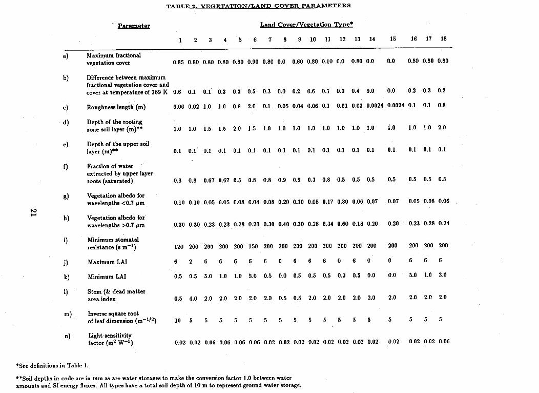
Table 2. Vegetation/Land-Cover Parameters .............. 21
Table 3. Soil Parameters ............. 27
iii
Page 5
LIST OF FIGURES
Page
Figure 1. Flow diagram showing major features of the surface param- 13eterization scheme employed in the NCAR CCM.
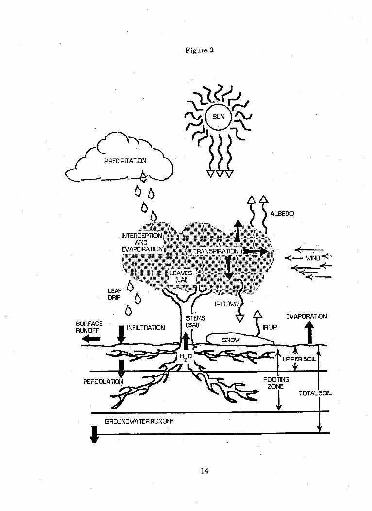
Figure 2. Schematic diagram illustrating the features included in the 14land-surface parameterization scheme used here.
Figure 3. Four land-surface types are shown to illustrate the flexi- 18bility of the parameterization of the land-surface scheme.The variation in the fraction of cover by vegetation ofthe soil surface is shown by (i) the relative width of the"plant" compared to the soil and (ii) the difference be-tween the "leaf" extents shown on the left-hand side ofthe "plant," the latter showing the temperature-dependentrange in cover. The differences in the stomatal resistancesare shown, schematically, by different size stomata on theright-hand side of the plant. The height of the plant indi-cates the vegetation roughness length except that the trop-ical forest is shown extending to only half the prescribedroughness length and the width of the "stem" indicates therelative importance of stems and dead matter in the groundcover. In addition to the parameters shown, the albedos(solar and near-infrared), the leaf area index, the foliageresistance to wind, and the plant sensitivity to photosyn-thetically active radiation are also parameterized.
iv
Page 6
LIST OF APPENDICES
Page
Appendix A. Fortran Symbols for Some Parameters in Model Code .... 60
Appendix B. Pointers Defining Location of Boundary Subroutine Variables . 65
v
Page 7
PREFACE
A comprehensive model of land-surface processes has been under development
suitable for use with various NCAR General Circulation Models (GCMs). Special
emphasis has been given to describing properly the role of vegetation in modifying
the surface moisture and energy budgets. The result of these efforts has been
incorporated into a boundary package, referred to as the Biosphere-Atmosphere
Transfer Scheme (BATS). The current frozen version, BATSle is a piece of software
about four thousand lines of code that runs as an offline version or coupled to
the CCM. It includes (i) assignment of land type and soil information to each
model grid square, (ii) calculation of soil, snow or sea-ice surface temperature in
response to net surface heating and depending on soil or snow heat capacity and
thermal conductivity, (iii) calculation of soil moisture, evaporation, and surface
and groundwater runoff, (iv) specification of vegetation cover in terms of fractional
ground shading and relative areas of transpiring and nontranspiring plant surfaces
for different types of land-use, (v) surface albedo in terms of soil moisture, vegetation
cover, and snow cover, including the shading of snow by vegetation, (vi) plant water
,budget including foliage and stem water storage, intercepted precipitation, and
transpiration as limited by stomatal resistance and soil dryness, (vii) surface drag
coefficients as a function of bulk Richardson number and vegetation cover, and (viii)
determination of foliage temperature in response to energy-balance requirements
and consequent fluxes of heat and moisture from the foliage to canopy air. Scientific
studies have been pursued over the last decade to better establish the importance
of various aspects of land-surface processes for climate and climate models and to
gain confidence in the utility of application of BATSle within a climate model. This
report describes the physical processes, current numerical parameterizations, and
some of the code structure of BATSle.
Robert E. DickinsonAugust 1993
vi
Page 8
ACKNOWLEDGMENTS
We thank K. Bluemel, A. Hahmann, X. Gao, F. Giorgi, A. Seth, J. Vaughn,
and Y. Liu for contribution to the improvement of the code or Technical Note.
We also thank Anji Seth for her careful review of the Technical Note. We thank
Stephanie Shearer for formatting and editing the text and NCAR's Graphics Ser-
vices and the Copy Center for their assistance in producing the color photograph
on the cover of this report. R. E. Dickinson's permanent affiliation is the University
of Arizona. A. Henderson-Sellers' permanent affiliation is Macquarie University,
School of Earth Sciences, New South Wales, Australia. P. J. Kennedy is a member
of the CGD Division at NCAR.
vii
Page 9
1. INTRODUCTION
The purposes of the biosphere-atmosphere transfer scheme (BATS), as cou-
pled with the NCAR Community Climate Model (CCM), are to (a) determine the
fraction of incident solar radiation that is absorbed by different surfaces and their
net exchange of thermal infrared radiation, (b) calculate the transfers of momen-
tum, sensible heat, and moisture between the earth's surface and atmospheric layers,
(c) determine values for wind, moisture, and temperature in the atmosphere, within
vegetation canopies, and at the level of surface observations, and (d) to determine
(over land and sea ice) values of temperature and moisture quantities at the earth's
surface. Included in the latter are the determination of the moisture content of soil,
the excess rainfall that goes into runoff, and the physical state of the moisture at
the surface, i.e., whether it is snow or water. To carry out these calculations, it
is necessary to prescribe a predominant land-surface category for each surface grid
point, and for those categories that have significant vegetative cover, to calculate
the exchanges of moisture and energy among the vegetation and the soil and the
air.
The earth's surface receives and emits various kinds of energy. The most im-
portant of these, from the viewpoint of physical processes, are (a) solar radiation,
absorbed after undergoing atmospheric absorption and reflection, as determined
by the radiative transfer subroutines and models of the surface albedo (depend-
ing on wavelength interval and solar zenith angle) (b) infrared radiation, emitted
from the surface according to eacT 4 , where e is the thermal emissivity, as is the
Stefan-Boltzmann constant, and T is the soil or vegetation temperature (down-
ward atmospheric flux is obtained from the detailed radiative transfer calculation
of the CCM or is parameterized); (c) sensible heat flux, by an aerodynamic trans-
fer formula as proportional to the difference between some surface and overlying
boundary-layer air temperatures; and (d) latent heat flux calculated similarly to
(c) but proportional to specific humidity differences. The net energy received at
the earth's surface melts snow, or warms the surface, or is conducted downward to
be stored in lower layers.
1
Page 10
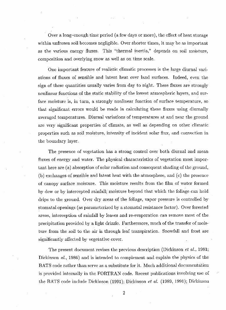
Over a long-enough time period (a few days or more), the effect of heat storage
within unfrozen soil becomes negligible. Over shorter times, it may be as important
as the various energy fluxes. This "thermal inertia," depends on soil moisture,
composition and overlying snow as well as on time scale.
One important feature of realistic climatic processes is the large diurnal vari-
ations of fluxes of sensible and latent heat over land surfaces. Indeed, even the
sign of these quantities usually varies from day to night. These fluxes are strongly
nonlinear functions of the static stability of the lowest atmospheric layers, and sur-
face moisture is, in turn, a strongly nonlinear function of surface temperature, so
that significant errors would be made in calculating these fluxes using diurnally
averaged temperatures. Diurnal variations of temperatures at and near the ground
are very significant properties of climate, as well as depending on other climatic
properties such as soil moisture, intensity of incident solar flux, and convection in
the boundary layer.
The presence of vegetation has a strong control over both diurnal and mean
fluxes of energy and water. The physical characteristics of vegetation most impor-
tant here are (a) absorption of solar radiation and consequent shading of the ground,
(b) exchanges of sensible and latent heat with the atmosphere, and (c) the presence
of canopy surface moisture. This moisture results from the film of water formed
by dew or by intercepted rainfall; moisture beyond that which the foliage can hold
drips to the ground. Over dry areas of the foliage, vapor pressure is controlled by
stomatal openings (as parameterized by a stomatal resistance factor). Over forested
areas, interception of rainfall by leaves and re-evaporation can remove most of the
precipitation provided by a light drizzle. Furthermore, much of the transfer of mois-
ture from the soil to the air is through leaf transpiration. Snowfall and frost are
significantly affected by vegetative cover.
The present document revises the previous description (Dickinson et al., 1981;
Dickinson al., 1986) and is intended to complement and explain the physics of the
BATS code rather than serve as a substitute for it. Much additional documentation
is provided internally in the FORTRAN code. Recent publications involving use of
the BATS code include Dickinson (1991); Dickinson et al. (1989, 1991); Dickinson
2
Page 11
and Kennedy (1991, 1992); Mearns et al. (1990); and Pitman et al. (1990). This
report is divided as follows: Section 2 describes how land-cover and soils data were
determined for the model and lists parameters dependent upon these classifications
(these are data sets that are not required for the offline BATSle model version,
but are needed as input for coupling to a GCM). Section 2 also describes specifi-
cation of land-surface albedo. (Section 3 summarizes what is involved in executing
the code of that BATS surface physics package linked to the CCM). Section 3 de-
scribes how soil temperature is calculated. Section 4 gives the determination of soil
moisture and snow cover for a nonvegetated grid square. Section 5 summarizes the
calculation of momentum drag coefficients including the modifications needed for
vegetation or for sea ice. Section 5 also describes how the model calculates sensible
and latent fluxes over a nonvegetated surface. Section 6 describes what parameters
are used to represent vegetation and how the model vegetation stores water. Sec-
tion 7 summarizes the calculation of soil moisture and snow cover in the presence
of vegetation. The appendices summarize some of the code notation.
Although the BATS treatment of surface processes is much more elaborate than
those of conventional GCMs, its treatment of individual processes is still conceptu-
ally much simpler than the most elaborate models available for such, in particular
for soil hydrology, plant water budgets, and snow physics.
3
Page 12
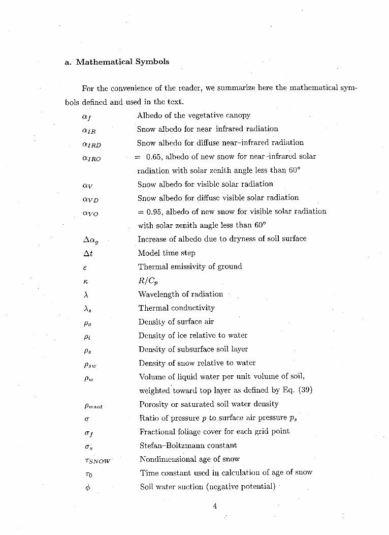
a. Mathematical Symbols
For the convenience of the reader, we summarize here the mathematical sym-
bols defined and used in the text.
af Albedo of the vegetative canopy
aIR Snow albedo for near-infrared radiation
CRRD Snow albedo for diffuse near-infrared radiation
aIRO = 0.65, albedo of new snow for near-infrared solar
radiation with solar zenith angle less than 60°
av Snow albedo for visible solar radiation
aVD Snow albedo for diffuse visible solar radiation
avo = 0.95, albedo of new snow for visible solar radiation
with solar zenith angle less than 60°
Aa - Increase of albedo due to dryness of soil surface
At Model time step
£~e Thermal emissivity of ground
ec ~ R/Cp
A Wavelength of radiation
As Thermal conductivity
Pa Density of surface air
Pi Density of ice relative to water
Ps Density of subsurface soil layer
Psw Density of snow relative to water
Pw Volume of liquid water per unit volume of soil,
weighted toward top layer as defined by Eq. (39)
Pwsat Porosity or saturated soil water density
a -Ratio of pressure p to surface air pressure ps
af Fractional foliage cover for each grid point
as Stefan-Boltzmann constant
TSNOW Nondimensional age of snow
TO Time constant used in calculation of age of snow
4f) ~ Soil water suction (negative potential)
4
Page 13
kMAX Soil water suction for permanent wilting of plants
b0o Soil water suction for saturated soil
Tro Maximum transpiration that can be sustained
Tw Rate of transfer of water by diffusion to the upper soil
layer from the lower; subscript zero denotes rate in the
absence of gravity
a Fraction of sea ice covered by leads
ci = Specific heat of ice _ 0.45 cW
Cs Specific heat of subsurface layer
Csw = 0.49 cw, specific heat of snow for unit snow density
Cw = 4.186 x10 6 J m - 3 K- 1, specific heat of water
CA,F,V Various bulk conductances as defined in the text
die Equivalent water depth of snow
dice Depth of ice
ds = 10 Sc/P = 10 x snow depth
f Ratio of soil evaporation to potential evaporation
fd Fraction of vegetation that is green and unwetted
fw Fraction of wet foliage
fsNOW Fraction of grid square covered by snow
f(ZEN) Increase of snow albedo due to solar zenith
exceeding 60°
g Acceleration due to gravity
hs = (Sg + (FIR - FIR)- F - L,sFq - LfSm), heat
balance at the surface
k von Karman constant
ks Soil or snow thermal diffusivity
pS Surface air pressure
Pi Lowest model level air pressure
q Specific humidity
qa Lowest model level water-vapor specific humidity
qaf Water-vapor specific humidity of the air within the foliage
5
Page 14
qg Soil surface water-vapor specific humidity
qg,s Saturated specific humidity at soil surface temperature
qs Water-vapor specific humidity inside the leaves
r a Aerodynamic resistance factor (1/(CfUaf))
rs Stomatal resistance factor
rTa Resistance to heat or moisture transfer through the
laminar boundary layer at the foliage surface
rF = rea/(afLsAI), bulk foliage resistance
rv Average resistance for transfer of water vapor from
foliage due to stomatal and aerodynamic resistance
of the foliage surface
rl Rate of "snow aging" due to grain growth from vapor
diffusion
r2 Rate of "snow aging" due to melt water
r3 Rate of "snow aging" from dirt and soot
r" Fraction of potential evaporation from a leaf
s Volume of water in soil divided by volume of
water at saturation
si Soil water as defined above in layer i
SW Soil water as defined above at permanent wilting point
S8 Stw/Stwmax
S1 Srw/Srwmax
S2 Ssw/Sswmax
t Time
ul Lowest model level west-to-east wind component
u* Friction velocity (pU*2 = surface momentum flux)
vl Lowest model level south-to-north wind component
zo Roughness length
zl 'Height of lowest model level
ALBG Albedo for bare soil
ALBL Albedo of plants for near infrared radiation
6
Page 15
ALBS Albedo of plants for visible radiation
ALBGO Albedo for wet bare soil
B Soil parameter defining change in soil water
potential and hydraulic conductivity with soil water, a
function of soil texture; also used as a symbol to represent
forcing of surface soil
Cf Coefficient of transfer between foliage and air in the
foliage
CP Specific heat of air
Cs Constant in snow albedo calculation (= 0.2)
CD Surface drag coefficient
CD,F Average momentum transfer coefficient over the grid
square in the presence of vegetation
CDH Aerodynamic transfer coefficient for heat
CDN Drag coefficient for neutral stability
CDVEG Aerodynamic drag coefficient for the canopy
CDW Aerodynamic transfer coefficient for water vapor
CN, Cs Constants in snow albedo calculation (= 0.5, 0.2)
C(ZEN) Cosine of the solar zenith angle
D Average diffusivity for water, flow through soil
Df Characteristic dimension of foliage elements in direction
of wind flow
Ds Rate of excess snow dropping from leaves per unit land area
DW Rate of excess water dripping from leaves per unit land area
Dmin Minimum value of soil diffusivity
Dmax = BOK(/pwm, maximum value of soil diffusivity
Ea,f,g Water flux per unit land area; f refers to origin at
foliage, g at ground, and a to the total flux; a
superscript N, in Eq. (77)-(84), refers to the flux
at the Nth iteration for leaf temperature
Etr Transpiration
7
Page 16
Maximum transpiration the vegetation can sustain
Heat conduction through snow-covered sea ice or bare
sea ice
Atmospheric sensible heat flux from ground to atmosphere
Moisture flux from ground to atmosphere
Sustainable moisture flux through the soil surface,
i.e., maximum as limited by diffusion
Fraction of vegetation covered by snow
Visible radiation incident at the top of the canopy
Snow age factor
Net long-wave radiation flux from atmosphere to bare
ground
Seasonal variation of vegetation cover with temperature
(Eq. lb)
Net water applied to the surface (Pr + Sm - Fq) in
absence of vegetation
Heat conduction rate from surface to underlying reservoir
Heat flux per unit land area to the atmosphere; f refers
to origin at foliage, g at ground, a to total flux
Hydraulic conductivity of soil
Saturated soil hydraulic conductivity, equivalent to
downward flow rate for saturated soil due to gravity
Land use/vegetation type in model
Unwetted fraction of leaf-stem area free to transpire
Latent heat of fusion
Latent heat of sublimation
Latent heat of evaporation
Either L, or LS, depending on whether Tg is greater
than freezing or not
Ratio of wetted leaf stem area to total leaf stem area
exchanging water with the atmosphere
8
Etrmx
FC
Fs
Fq
Fqm
Fsn
Fvi
FAGE
FT FTIR IR
FSEAS(T)
G
GHEAT
Ha,f,g
K
Ko
KVEG
Ld
Lf
Ls
Lv
LVIS
Page 17
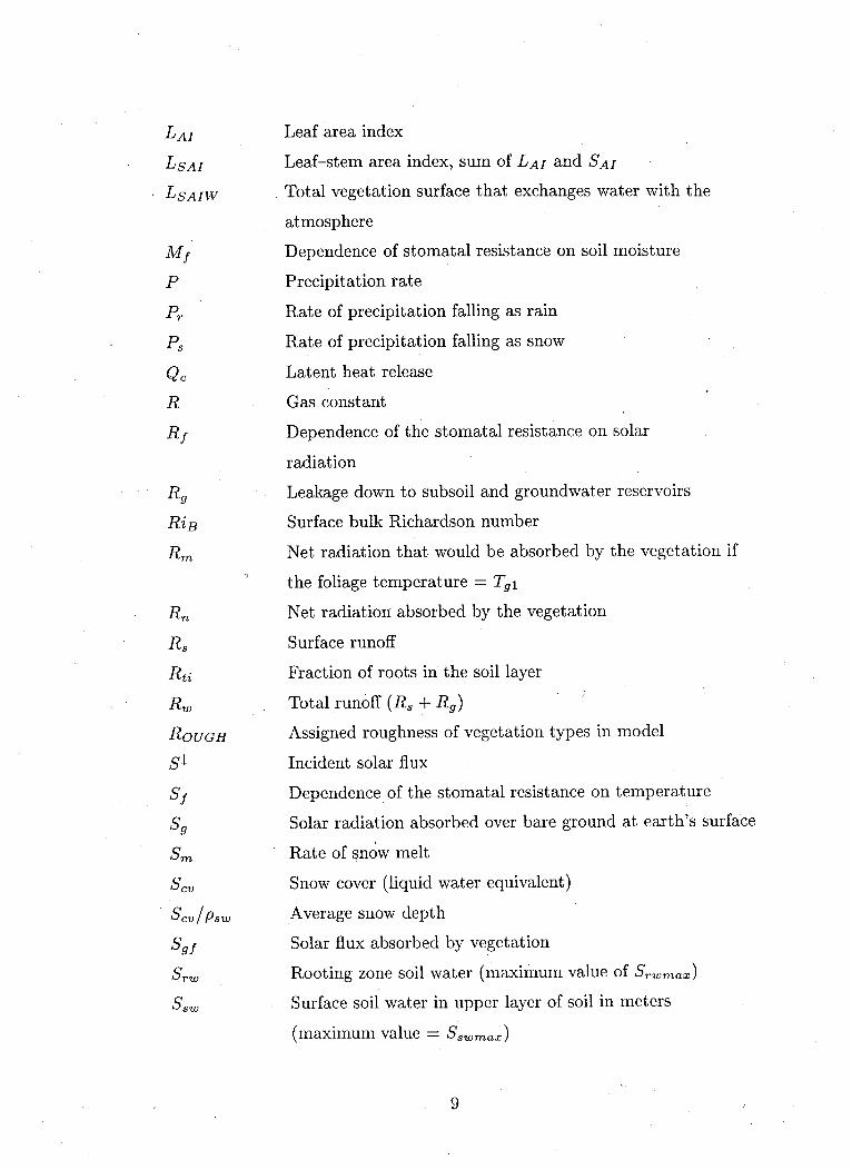
LAI Leaf area index
LSAI Leaf-stem area index, sum of LAI and SAI
LSAIW Total vegetation surface that exchanges water with the
atmosphere
Mf Dependence of stomatal resistance on soil moisture
P Precipitation rate
Pr Rate of precipitation falling as rain
PS Rate of precipitation falling as snow
Qc Latent heat release
R Gas constant
Rf Dependence of the stomatal resistance on solar
radiation
Rg Leakage down to subsoil and groundwater reservoirs
RiB Surface bulk Richardson number
Rm Net radiation that would be absorbed by the vegetation if
the foliage temperature = Tgl
Rn Net radiation absorbed by the vegetation
Rs Surface runoff
Rtu Fraction of roots in the soil layer
Rw Total runoff (Rs + Rg)
ROUGH Assigned roughness of vegetation types in model
S 1 Incident solar flux
Sf Dependence of the stomatal resistance on temperature
Sg Solar radiation absorbed over bare ground at earth's surface
Sm Rate of snow melt
Scv Snow cover (liquid water equivalent)
Scv/psw Average snow depth
Sgf Solar flux absorbed by vegetation
Srw Rooting zone soil water (maximum value of Srwmax)
Ssw Surface soil water in upper layer of soil in meters
(maximum value = Sswmax)
9
Page 18
StW Total water in soil column of soil (maximum
value = Stwmax)
SAI Stem area index
Taf Temperature within the foliage layer
Tc Reference temperature for deciding whether precipitation is
rain or snow
Tf Temperature of foliage
Tg1 Surface soil temperature
Tg2 Subsurface temperature (depth of about 0.2 m)
Tg3 Deep soil temperature (depth of about 2 m = annual average)
Tm = 273.16 K, the melting or freezing temperature of pure water
TB Approximate freezing point of sea water
Ta Air temperature of lowest model layer x(pl/ps)-.
Uaf Magnitude of wind within the foliage layer
Uc Subgrid-scale horizontal convection velocity
Va = (u2 + v + U2) 1 / 2, strength of wind at the anemometer level
Vf Dependence of stomatal resistance on vapor pressure deficit
Wdew Total water stored by canopy per unit land area
WDMAX Maximum water the canopy can hold
WLT Soil dryness (or plant wilting) factor
Wm1 Rate of melting (freezing if negative) of surface soil water
Wm2 Rate of melting (freezing if negative) of subsurface soil water
Zu Depth of upper soil layer, fixed at 0.10 up to now
Zr Depth of soil rooting layer, varies typically from
0.5 to 2 m in thickness as a function of vegetation
cover and/or land use
Zt Depth of total soil zone
10
Page 19
2. DATA AND INTERFACE REQUIREMENTS
FOR BATS COUPLED TO THE NCAR CCM
a. Overview and Coupling Requirements
To integrate BATS with the CCM or other atmospheric global or mesoscale
model, a number of data fields must be supplied and other fields passed between
BATS and the CCM/GCM at each model time step, as illustrated in Figure 1.
The atmospheric model defines from read in data sets a distribution of land
points, including elevation, sea ice coverage, and ocean surface temperatures; the
latter two can vary seasonally. A distribution of net energy fluxes over the ocean
may also be prescribed as derived from a previous simulation and used for a flux
corrected slab ocean temperature calculation. Data is read in for each land point,
describing its assumed dominant vegetation cover, soil texture and soil color. Some
vegetation and soil properties that vary interactively with BATS must be made
available for calculation of albedo.
Interactive properties entering the albedo calculation include fraction of vege-
tation coverage, soil moisture, snow cover and snow age. The albedo routine must be
tailored to match surface solar radiative fluxes provided by the atmospheric model.
In particular, it must match the spectral intervals assumed by the model and treat
separately direct solar beam and diffuse radiation.
Because the land versus ocean distributions of the prescribed data sets may
not match those of CCM1, checks are made to provide soil and vegetation data to
any CCM1 points that are classified land in the CCM but ocean in the land use
data set. In CCM2, the prescribed data sets were edited to match the land versus
ocean of the model. All the needed CCM fields are passed into a data structure
adopted from an earlier NCAR GCM. The lowest model temperature is multiplied
by (Jk for use as a "potential temperature." A routine named SOLBDC is called to
obtain soil hydrological properties as a function of the soil-data fields. The routine
BNDRY is then called to enter the main boundary package. Finally, the fields are
transferred back into a form suitable for the CCM. Note, in particular, that we pass
heat, moisture, and momentum fluxes evaluated for surface temperatures present
at the finish of the boundary package for use in the vertical diffusion routine.
11
Page 20
Subroutine BNDRY calls individual physical process subroutines and evaluates
parameters common to several routines, as indicated in Figure 2. In particular, it
provides the relative soil moisture from the model moisture and maximum soil
moisture storage. It calls subroutine DRAG to obtain transfer coefficients between
the lowest model layer and the surface (canopy plus ground). The coefficients
depend on the lowest model altitude, surface roughness zo-determined from surface
cover-and a bulk Richardson number calculated from the strength of the lowest
model-layer winds and the temperature difference between surface and lowest model
layer.
12
Page 21
Figure 1
- OCEAN - TEST WHETHER OVER OCEAN, CONTINENT OR SEA ICE
CALCULATE C D AND MOMENTUM DRAG
4CONTINENT OR SEA ICE
(COMPUTE SURFACE TEMPERATURE)
TEST IF VEGETATION
NO YES
. .NO VEGETATION COMPUTE LEAF AREA, WIND IN CANOPY,
CONTINENT OTHER VEGETATION PARAMETERS.
STOMATAL RESISTANCE
4(ADJUST STOMATAL RESISTANCE SO THAT -----
TRANSPIRATION DOES NOT EXCEED
WATER FLOW TO ROOTS)
COMPUTE TRANSPIRATION AND LEAF
EVAPORATION RATES, DEW FORMATION,
LEAF TEMPERATURE
TEST IF SEA ICE TEST IF CNVERGESTEST IF CONVERGES
YES NO NO_-- ITERAT.. : ̂ ,, IYES
· n^ ^^^ -^~ ~DETERMINE SOIL TEMPERATURE,
;ULATE SEA ICE TEMPERATURESOIL MOSTURE, RUNOFFAND SNOW COVERFLUXES TO ATMOSPHERE,ANDSNOWCOVER
WING FOR LEADS
- COMPUTE SENSIBLE AND LATENT FLUXES TO ATMOSPHERE
AND DAILY AVERAGE DIAGNOSTICS
13
SEAICE OR
OVER (
CALC
ANDI
ALLO'
f
I
.
rE
. I r
Page 22
Figure 2
I tALBEDO
14
Page 23
The vegetation part of the code is only executed for grid squares with vegeta-
tion cover greater than 0.001. A mean wind within the canopy is obtained from the
mean wind outside the canopy times the square root of the drag coefficient, which
equals the friction velocity u*. The coefficient of transfer of heat and momentum
from leaves is calculated. Foliage water is modified by intercepted rainfall. The
temperature of the foliage (leaves) is calculated. Any rain or snow intercepted by
leaves in excess of their maximum capacity is determined as falling to the ground
and saved for soil-water or snow-budget calculations.
Returning to a calculation for all surfaces, we calculate rain or snow incident
on the ground (minus any that was intercepted by the foliage) and partition soil
evaporation into that from soil water and that from overlying snow. Routines
are called to calculate the sea ice or the ground temperature and the budgets of
snow cover and soil water. The updated temperatures, soil moisture, and foliage
transpiration are used to determine net fluxes of heat and momentum from the
surface to the lowest atmospheric model layer.
Surface-air properties are estimated for comparison with observations by using
boundary-layer theory to interpolate between lowest model layer temperature and
surface (ground, canopy-air or ocean). For connection to an overlying atmospheric
model, temperature is evaluated at 10 m over ocean and 1.3 m over land, where
it is assumed measured within a plot of short grass, embedded in the given cover
type. The approximate formula used is
T, Taf + T,
where
Taf = Taf, if vegetated,
Taf = Tg, if nonvegetated,
AT (T - Taf)ZDELT,
15
Page 24
ZDELT = minimum of(1, b/[log(z /zo)] 2 ),
where zo = 0.01 m, and over land b = 4.8(CDICDN)1/ 2 where CD is the drag
coefficient at z1 and CDN is its value for neutral conditions.
b. Land-Type Assignment
Currently, three global land-surface archives have been designed for incorpora-
tion into climate models-the vegetation data set of Olson et al. (1983), the vegeta-
tion and cultivation data of Matthews (1983, 1984) and the land use and soils data
of Wilson (1984), described in Wilson and Henderson-Sellers (1985). The latter
land-use data archives were used in the construction of a land-type data set for the
CCM at R-15 resolution. The Olson et al. (1983) data has been used to construct
a land use data set at T-42 resolution for use in CCM2. The implementation of the
soils data of Wilson (1984) is described in the following subsection.
Matthews (1983, 1984) defines 31 classes of natural land type and prescribes
the intensity of cultivation for each 1 - x -1° grid element. Wilson (1984) also uses
base resolution of 1° x 1° but defines two land-cover types for each land element-
primary > 50% of the grid square, and secondary < 50% but > 25%. She uses
53 land-cover classes including a number of cultivation categories. To simplify
somewhat the CCM land-cover specification, both data archives were reduced to
percentages of the 18 more basic land-cover classes shown in Table 1. Examples of
the role of these different use classes are given in Figure 3.
16
Page 25
Table 1. Vegetation/Land-Cover Types
1. Crop/mixed farming
2. Short grass
3. Evergreen needleleaf tree
4. Deciduous needleleaf tree
5. Deciduous broadleaf tree
6. Evergreen broadleaf tree
7. Tall grass
8. Desert
9. Tundra
10. Irrigated crop
11. Semi-desert
12. Ice cap/glacier
13. Bog or marsh
14. Inland water
15. Ocean
16. Evergreen shrub
17. Deciduous shrub
18. Mixed Woodland
17
Page 26
Figure 3
Deeper soil
Largeseasonal
rangein
fractionalcover
Potential rangeIn
fractional covernot achieved
becausetemperaturevaries little
Most rootsin
surface layer
Many stemsand
dead matter
Smallfractional
cover
Most rootsin
lower layer
SmallO * _ ^P 0 I
Large Few roots symaal«fractional In resistance
cover lower layer
~.- IXm- - T
SHORTGRASS
TUNDRA IRRIGATED. CROP
TROPICALFOREST
18
r
l ~~~~~..wwmm
. I
e
Page 27
Data sets at the R-15 resolution of approximately 4.5° x 7.5° were derived
from each of the 1°-sets and initially in terms of percentages of the 17 basic types
in each grid element. Each grid element was assigned a dominant type except when
use of type 18 (mixed woodland) seemed more appropriate.< The dominant land
types inferred from each data set were compared and if the classifications agreed,
the result was incorporated into- the final R-15 data set. At some model grid squares,
differences occurred between the Matthews and the Wilson data sets, and two al-
ternative or combined steps were taken. First, an average (of the two percentage
components) was established and second, a comparison was made between this aver-
age and the ecotype classification of Olson et al. (1983), and subjective assessment
was made as to what classification to use. The resultant archive is of 18 land-use
classes defined on the model mesh. These 18 classes of land cover are used to define
a wide variety of land surface, hydrological, and vegetation properties as described
below.
The T-42 data set was derived by simply associating one of the 18 data types
with each of the vegetation types of Olson et al. (1983), and the 0.5° data was
accumulated with model grid cells and the dominant type in each cell selected.
For each grid point, a value KVEG is read into the model: KVEG = O for all
ocean grid points; KVEG = 1 for all points with arable/mixed farming, etc. The
assigned roughness length ROUGH (given in Table 2) is used as the aerodynamic
roughness, and the fraction of a grid square covered by snow fsNOW is inferred
according to the formula,
fsyow = fsN/(l + fsN), (la)
with
fsN = 0.1 SCV/(psw x ROUGH). (lb)
The quantity Scv/(ps,) is the average snow depth and ROUGHIO.1 is about half
the average vertical extent of the surface objects. The quantity fsNO\, calculated
separately for the vegetated and nonvegetated parts of a grid square, determines
what fraction of the area has the albedo of snow versus that of no snow. Over
19
Page 28
vegetated areas, all vegetation covered by the snow pack is neglected by reducing
the fraction of vegetation cover defined in subsection (b) by the factor (1 - fsNow).
For each land cover type, several vegetation parameters are required as indi-
cated in Table 2. Besides roughness and albedo (discussed in next section) BATS
requires a fractional vegetation af and a leaf and stem area index LAI and SAI.
The fractional vegetation and LAI range between minimum and maximum values
according to a dependence on subsoil temperature
FSEAS(Tg2) =1 - 0.0016 x (298.0 - Tg2) 2 (Ic)
when
273.16 < Tg2 < 298
The fractional vegetation in the presence of snow is reduced by a factor (1- fsNow)
so that snow covered vegetation does not interact with the atmosphere. It is a
current research topic to make these parameters more interactive with the model
climate.
A number of the land-surface parameters defined as a function of land-cover
type should, strictly, be made functions of soil type. However, for the present
implementation, rooting ratios and upper and total soil depths (illustrated in Figure
1) remain a function of land-cover type only (Table 2). A number of parameters
do vary with soil type and are described in the next subsection.
20
Page 29
TABLE 2. VEGETATION/LAND COVER PARAMETERS
Land Cover/Vegetation Type*
Maximum fractionalvegetation cover
Difference between maximumfractional vegetation cover andcover at temperature of 269 K
Roughness length (m)
Depth of the rootingzone soil layer (m)**
Depth of the upper soillayer (m)**
Fraction of waterextracted by upper layerroots (saturated)
Vegetation albedo forwavelengths <0.7 pm
Vegetation albedo forwavelengths >0.7 pm
Minimum stomatalresistance (s m- 1)
Maximum LAI
Minimum LAI
Stem (& dead matterarea index
Inverse square rootof leaf dimension (m- 1/2 )
1 2 3 4 5
0.85 0.80 0.80 0.80 0.80
0.6 0.1 0.1
0.06 0.02 1.0
1.0 1.0 1.5
0.1 0.1 0.1
0.3
1.0
1.5
0.1
0.3
0.8
2.0
0.1
6 7
0.90 0.80
0.5
2.0
1.5
0.1
0.3
0.1
1.0
0.1
8 9 10 11
0.0 0.60 0.80 0.10
0.0 0.2 0.6 0.1
0.05 0.04 0.06 0.1
1. 1.0 1.0 1.01
0.1 0.1 0.1 0.1
12 13 14 15
0.0 0.80 0.0 0.0
0.0 0.4 0.0
0.01 0.03 0.0024
1.0 1.0 1.0
0.1 0.1 0.1
0.0 0.2
0.0024 0.1
1.0 1.0
0.1. 0.1
0.3 0.8 0.67 0.67 0.5 0.8 0.8 0.9 0.9 0.3 0.8 .0.5 0.5 0.5 0.5
0.10 0.10 0.05 0.05 0.08 0.04 0.08 0.20 0.10 0.08 0.17 0.80 0.06 0.07 0.07
0.30 0.30 0.23 0.23 0.28 0.20 0.30 0.40 0.30 0.28 0.34 0.60 0.18 0.20 0.20
120 200 200 200 200 150 200 200 200 200 200 200 200 200 200
6 2 6 6 6 6 6 0 6 6 6 0 6 0 0
0.5 0.5 5.0 1.0 1.0 5.0 0.5 0.0 0.5 0.5 0.5 0.0 0.5 0.0 0.0
0.5 4.0 2.0 2.0 2.0 2.0 2.0 0.5 0.5 2.0 2.0 2.0 2.0 2.0 2.0
10 5 5 5 5 5 5 5 5 5 5 5 5 5 5
n) Light sensitivityfactor (m2 W- 1) 0.02 0.02 0.06 0.06 0.06 0.06 0.02 0.02 0.02 0.02 0.02 0.02 0.02 0.02 0.02 0.02 0.02 0.06
*See definitions in Table 1.
**Soil depths in code are in mm as are water storages to make the conversion factor 1.0 between water
amounts and SI energy fluxes. All types have a total soil depth of 10 m to represent ground water storage.
Parameter
16
0.80
17 18
0.80 0.80a)
b)
c)
d)
e)
f)
g)
h)
i)
J)
k)
1)
m)
0.3
0.1
1.0
0.1
0.2
0.8
2.0
0.1
0.5
0.06
0.24
200
6
3.0
2.0
5
0.5 0.5
0.05 0.08
0.23 0.28
200 200
6 6
5.0 1.0
2.0 2.0
5 5
-II
Page 30
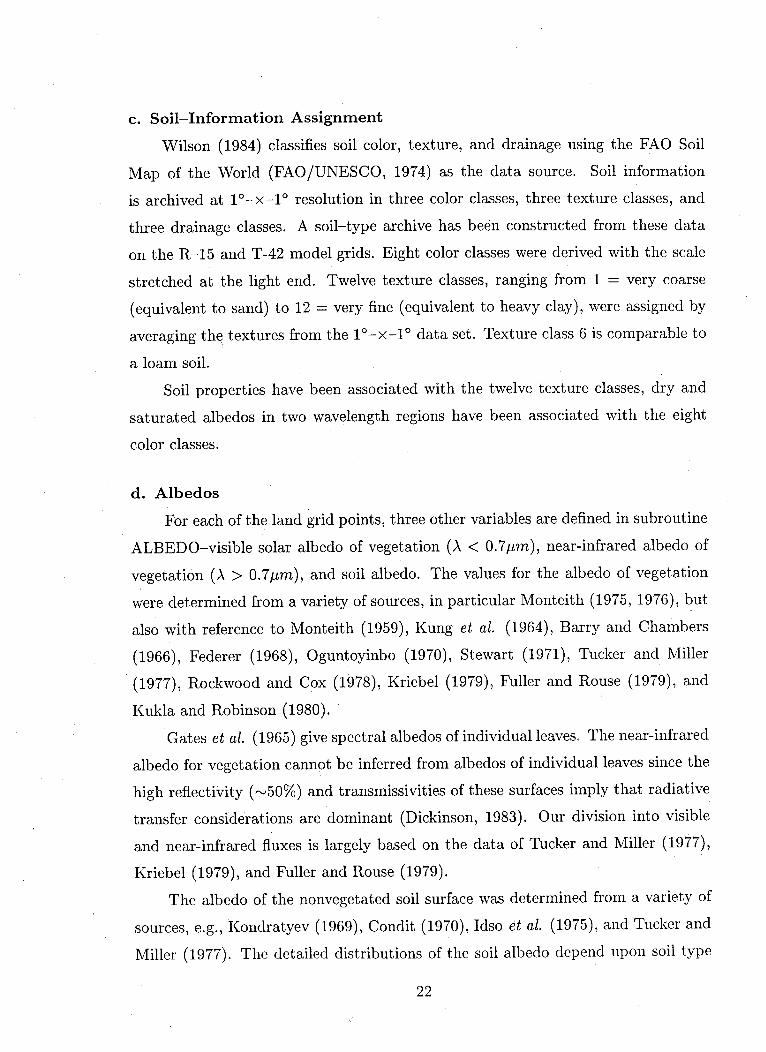
c. Soil-Information Assignment
Wilson (1984) classifies soil color, texture, and drainage using the FAO Soil
Map of the World (FAO/UNESCO, 1974) as the data source. Soil information
is archived at 1°-x-1 ° resolution in three color classes, three texture classes, and
three drainage classes. A soil-type archive has been constructed from these data
on the R-15 and T-42 model grids. Eight color classes were derived with the scale
stretched at the light end. Twelve texture classes, ranging from 1 = very coarse
(equivalent to sand) to 12 = very fine (equivalent to heavy clay), were assigned by
averaging the textures from the 1l-x-l1 data set. Texture class 6 is comparable to
a loam soil.
Soil properties have been associated with the twelve texture classes, dry and
saturated albedos in two wavelength regions have been associated with the eight
color classes.
d. Albedos
For each of the land grid points, three other variables are defined in subroutine
ALBEDO-visible solar albedo of vegetation (A < 0.7/m), near-infrared albedo of
vegetation (A > 0.7pum), and soil albedo. The values for the albedo of vegetation
were determined from a variety of sources, in particular Monteith (1975, 1976), but
also with reference to Monteith (1959), Kung et al. (1964), Barry and Chambers
(1966), Federer (1968), Oguntoyinbo (1970), Stewart (1971), Tucker and Miller
(1977), Rockwood and Cox (1978), Kriebel (1979), Fuller and Rouse (1979), and
Kukla and Robinson (1980).
Gates et al. (1965) give spectral albedos of individual leaves. The near-infrared
albedo for vegetation cannot be inferred from albedos of individual leaves since the
high reflectivity (-50%) and transmissivities of these surfaces imply that radiative
transfer considerations are dominant (Dickinson, 1983). Our division into visible
and near-infrared fluxes is largely based on the data of Tucker and Miller (1977),
Kriebel (1979), and Fuller and Rouse (1979).
The albedo of the nonvegetated soil surface was determined from a variety of
sources, e.g., Kondratyev (1969), Condit (1970), Idso et al. (1975), and Tucker and
Miller (1977). The detailed distributions of the soil albedo depend upon soil type
22
Page 31
and soil wetness. However, for vegetation cover af of 0.80 or more, relatively little
short-wave radiation reaches the ground so that these parameterizations become
secondary.
The values for vegetation albedo presently used in subroutine ALBEDO are
listed in Table 2. We have not been able to find much data on the albedos of branches
and brown vegetation as contrasted to green (besides Federer, 1968, 1971), but we
assume that it is the same as green. It appears that trunks and branches may have
lower albedos by as much as 0.05, that red or brown leaves may have higher albedos
by a much as 0.05, and that the spectral variation of albedo for either of these will
differ from that of green leaves.
The albedo for bare soil ALBG is taken to be
ALBG = ALBGO + Aag(Ssw), (2a)
where ALBGO is the albedo for a saturated soil and where the increase of albedo
due to dryness of surface soil is given for A < 0.7pm as a function of the ratio of
surface soil water content Ssw to the upper soil layer depth Z,,
Acg(Sw) = 0.01(11 - 40Ss/Z,) > 0. (2b)
This formulation is chosen so that soil albedos range in a nonlinear fashion between
the saturated and dry values listed above. The term Sw becomes small (<0.025
m) before the soil albedo shows a significant increase. Moisture is retained around
the soil grains until -80% dryness occurs. The soil albedos for A > 0.7gm are twice
those for A < 0.7,m. Dry and saturated soil albedos for the eight color classes used
are shown in Table 3.
e. Snow Albedos
Snow albedos depend on spectral mix of the incident radiation/solar zenith
angle, soot loading of the snow, snow depth, and grain size. Marshall (1989) has
carefully developed a treatment of snow albedo with some advanced features not
yet incorporated into BATS including combining the zenith dependence with grain
size and depth dependence with soot loading.
23
Page 32
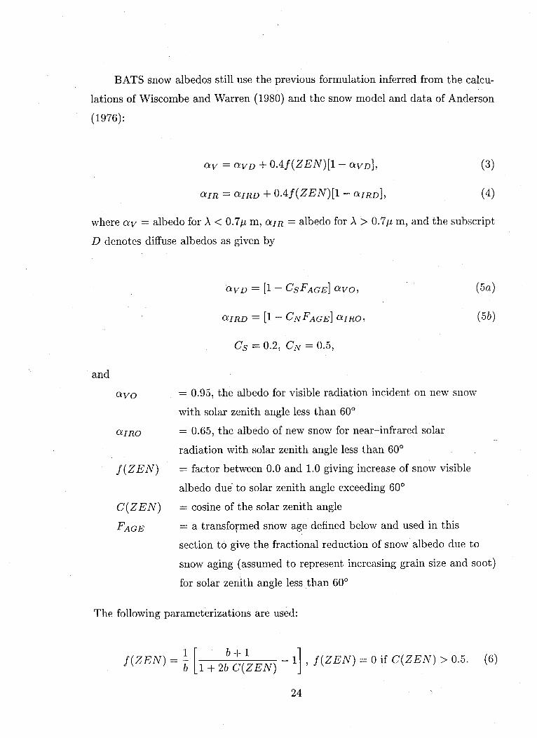
BATS snow albedos still use the previous formulation inferred from the calcu-
lations of Wiscombe and Warren (1980) and the snow model and data of Anderson
(1976):
av = aVD + 0.4f(ZEN)[1 - aVD], (3)
IR = aIRD + 0.4f (ZEN)[1 - aIRD], (4)
where av = albedo for A < 0.7,1 m, aIR = albedo for A > 0.7/u m, and the subscript
D denotes diffuse albedos as given by
aVD = [1 - CSFAGE] aVO, (5a)
aIRD = [1- CNFAGE] aIRO, (5b)
Cs 0.2, CN = 0.5,
and
avo = 0.95, the albedo for visible radiation incident on new snow
with solar zenith angle less than 60°
aIRO = 0.65, the albedo of new snow for near-infrared solar
radiation with solar zenith angle less than 60°
f(ZEN) = factor between 0.0 and 1.0 giving increase of snow visible
albedo due to solar zenith angle exceeding 60°
C(ZEN) = cosine of the solar zenith angle
FAGE = a transformed snow age defined below and used in this
section to give the fractional reduction of snow albedo due to
snow aging (assumed to represent increasing grain size and soot)
for solar zenith angle less than 60°
The following parameterizations are used:
f( N) = [ + 2b (ZEN)- , f(ZEN) = 0 if C(ZEN) > 0.5. (6)b [1± 2b C(ZEN) J
24
Page 33
Equation (6) has the property for all b that it vanishes at C(ZEN) = 0.5 and
is unity at C(ZEN) = 0 (sun on the horizon); b is adjustable to best available
data-for now b = 2.0.
Snow albedo decreases with time due to growth of snow grain size and accu-
mulation of dirt and soot. We parameterize the decrease term FACGE in the above
by
FAGE = TSNOW/[1 + TSNOW]. (7)
The nondimensional age of snow TSNOW is incremented as a model prognostic
variable as follows:
1/TSNOW = To 1(rl + r2 + r3)At, (8)
where T0 1 =1 x 10⁻⁶ -1 ,
r= exp [5000 (27316 T- l[ ( 273.1 6 1g
r2 r ° < 1,
and
r3 = 0.01 over Antarctica, = 0.3 elsewhere.
The term r1 represents the effect of grain growth due to vapor diffusion, the
temperature dependence being essentially proportional to the vapor pressure of
water.
The term r 2 represents the additional effect near and at freezing of melt water
and r3 the effect of dirt and soot.
A snowfall of 0.01 m liquid water is assumed to restore the surface age, hence
albedo, to that of new snow. Since the precipitation in one model time step will
generally be less than that required to so restore the surface when it snows for a
25
Page 34
given time step, we reduce the snow age by a factor depending on the amount of
the fresh snow in m, APs, as follows:
NOW- = (rSNvOW + /ArSNOW)(l- 100APs), TSNow > 0, (9)
where A'TSNOW is defined as in Eq. (8).
26
Page 35
TABLE 3. SOIL PARAMETERS
I/FUNCTIONS OF TEXTURE
Parameter Texture Class (from sand (1) to clay (12))
1 2 3 4 5 6 7 8 9 10 11 12
a) Porosity (volume ofa) Porosity (volume of
voids to volume of soil)
b) Minimum soil suction (mm)
c) Saturated hydraulicconductivity (mm s-l)
0.33 0.36 0.39 0.42 0.45 0.48 0.51 0.54 0.57 0.60 0.63 0.6O
30 30 30 200 200 200 200 200 200 200 200 200
0.2 0.08 0.032 0.013 8.9 x10 3 6.3 x10 3 4.5 x10 3 3.2 x10⁻³ 2.2 x10 3 1.6 x10⁻³ 1.1 x10⁻³ 0.8 x10⁻³
d) Ratio of saturated thermalconductivity to that of loam
e) Exponent "B" defined in Clapp& Hornberger (1978)
f) Moisture content relative tosaturation at whichtranspiration ceases
1.7 1.5 1.3 1.2 1.1
3.5 4.0 4.5 5.0 5.5
0.088 0.119 0.151 0.266 0.300
1.0 0.95 0.90 0.85 0.80 0.75
6.0 6.8 7.6 8.4 9.2 10.0
0.70
10.8
0.332 0.378 0.419 0.455 0.487 0.516 0.542
II/FUNCTIONS OF COLOR
Parameter Color (from light (1) to dark (8)
1 2 3 4 5 6 7 8
a) Dry soil albedo< 0.7 pim> 0.7 pm
b) Saturated Soil Albedo< 0.7 pm> 0.7 pm
0.23 0.22 0.20 0.18 0.16 0.14 0.12 0.100.46 0.44 0.40 0.36 0.32 0.28 0.24 0.20
0.12 0.11 0.10 0.09 0.08 0.07 0.06 0.050.24 0.22 0.20 0.18 0.16 0.14 0.12 0.10
0% Is ^ AX 9 A ,.AI
Page 36
3. SOIL TEMPERATURE
The basis of the soil temperature model is described in Dickinson, (1988) which
generalized the force restore method of Deardorff (1978). The following parameters
are needed:
A = thermal conductivity
d = 2ir/86400 diurnal frequency
ya = vd/365 seasonal frequency
At = time step in s
h (Sg +F FI -FIR- FS F -L ,FqLfSm)
the net soil surfaces heat impact, where
Sg = Solar flux absorbed over bare ground at earth's surface
F 1 - FR = Net IR (long wave) flux from atmosphere to bare ground
Fs = Atmospheric sensible heat flux from ground to atmosphere
Fq = Atmospheric moisture flux from ground to atmosphere
L,s = Latent heat of evaporation or sublimation
Lf = Latent heat of fusion
Qsf = LfWm2Cl/(pscsdlc 2) = Rate of subsoil temperature change
because of melting or freezing
Sm = Rate of snow melt
a. Surface Soil Temperature
Surface soil temperature Tgl is calculated from the following differential equa-
tion
tOTg(cat - + 2ATgl=B (10)atwith the coefficients to be described below; B includes a term proportional to net
surface heating.
BN+1 = BN + B'(T+1 - Tg) (ila)
where T°1 is the initial value of temperature from the previous time step (expression
corrects latent and sensible fluxes to current temperature) and
28
Page 37
A = 0.5 vd At
B = BCOEF hs + Vd At Tg2 (llc)
where hs is the net surface heating, and
BCOEF = fSNOW BCOEFS + (1 - fsNOw) BCOEFB (lid)
where fsNOW is defined by Eq. (la). Also
Vd At DdsBCOEFS = t Dd8 (lie)
(Ps Cs)s ksn
BCOEFB = 7Vd At Ddb ((Ps Cs)b ksb
and the diurnal penetration depths are
Dds = (- (11g)
2ksb) (h)Ddb -- cv Yd )(1h)
and where B' is the derivative of B with respect to temperature and is approximated
by the temperature dependence of sensible and latent heat fluxes, defined later. In
a more advanced approach where Tg is solved jointly with leaf temperatures (cf.
Section 6g), an additional term, is added to B correcting to Tf+ 1.
With Crank-Nicholson time differencing but using (11) to estimate B, we ad-
vance surface soil temperature from the Nth to N + ith time step (the change is
limited to at most ± 10°), using
TN+i = B + (C- A- B')Tgl (C +A- B')
d = thermal diffusivity of snow, k = thermal diffusivity of soil for diurnal wave,
derived from soil water of upper soil layer.
29
(11b)
Page 38
And,
C =(1+ FCT1) (13)
where FCT1 is an additional thermal inertia of freezing to be described below (17b).
Snow diffusivity is based on: Corps. of Engineers (1956), Yen (1969), and
Anderson (1976).
ksn = so Psw
where kso = (7.0 x 10⁻⁷/0.49) m 2 s 1 and the heat capacity is
(PsCs) = Psw sw
where
c - 0.49c,
is the specific heat per unit snow density, and where Psw is the density of snow
relative to water.
Snow density is assumed given by
Pw -=0.1 + 0.3FAGE (14)
where FAGE is the snow age factor.
Soil thermal diffusivity and heat capacity depend on soil moisture and texture
(following deVries, 1963). For non frozen (bare) soil,
(PsCs)b = (0.23 + PW)Cw (15)
(2.9pw + 0.04)kcksb (1 - 0.6p,)pw + 0.09 (16)
where
k = 10- 7m 2s- x RAT
30
Page 39
where RAT is the ratio of the thermal diffusivity for a given texture to that for
loam.
cw = 4.186 x 10⁶ J m- 3 K- 1
is the specific heat of water and Pw is the volume of water per unit volume of soil.
Separate p,'s are defined for the surface layer for the diurnal wave and for the root
zone layer for the annual wave.
Modified thermal properties are used for frozen soil, i.e.
ks 1.4 x 10⁶ m 2 s-l
and the contribution of water to psCs is reduced by 0.51 for that fraction of the
water that is frozen. It is assumed that water freezes uniformly between 0°C and
-4 0C.
The term FCT1 > 0 parameterizes the contribution of the latent heat of freezing
from the upper soil layer to surface energy balance, assuming this heating is given
by the term
Du Lf (Ssw-Fru F) Tg7a)
[Zu ] AT At
where AT = 40
so that
FCT1 = > (17b)ps cs AT Zu
The term Fru is the fraction of upper layer soil water that does not freeze. The
term in square brackets in (17a), which is 0(1), does not appear to be necessary
and should be omitted in future implementations.
31
Page 40
b. Snow Melt
In the presence of snow, snow melt is assessed from the energy required to
balance hs and change Tg, to 0°C. If positive, inferred latent heat of melting is
removed from hs, limited by the remaining snow cover. This is written
[B + (C- A- B')Tg - (C + A - B') x 273.16]bm == ------------------f.--D-------------------- [(18a)
Lf BCOEF
O < Sm < At Scv (18b)
The derivative of soil sensible and latent heat fluxes with respect to temperature
use to evaluate B' are estimated in the absence of vegetation by
aFsPa CD Cp Va (19a)
OT
aFq aqs (Tg1)" Pa CD Va fg (19b)a~T aOT
where fg is a soil wetness factor determined from the soil evaporation formulation
as the ratio of evaporation to that from a wet surface. In (19), we have neglected
the contribution of the temperature dependence of CD.
Estimates of flux derivatives with vegetation are described later. The flux
derivative terms (19) are used to correct Fs and Fq to the N + 1 time step to insure
energy conservation.
c. Subsurface Temperature
The subsurface temperature Tg2 is identified with the annual temperature wave
in calculating from force-restore corresponding to temperature at a depth of roughly
1 m. As described in Dickinson, (1988),
aTg2 Da(1 + FCT2 ) at 2 + 2 A2 T2 = 4 + Va At T + (20)
at Dd
where c4 is a coupling coefficient to soil untouched by annual wave. At present
C4 = 0, except under permafrost where we take, 4 = 1. T3 = 271.0. The term A 2
is
32
Page 41
DaA 2 = (c 4 + d) 0.5va At (21)
in the absence of snow,
Da ()/2 Dd (21a)Va
and in the presence of snow, both Da and Dd are weighted averages according to
the depth of the snow,
Dd = WTDS Dds + (1- WTDS) Ddb (21b)
Da = WTAS Das + (1- WTAS) Dab (21c)
with Das and Dab defined from Dd, and Ddb with the factor of (21a). The weights
for the snow contribution are
-2. ScvWTDS = [1- exp ( V )fsNow (21d)
Psw Ddb
-2. S)oWTAS = [1- exp (P D )]fsNow (21e)
Psw Dab
where
_ 2 Lf(Srw - Frr)FCT2 - Lf(S-F) > 0 (22)
ps cs AT Zr
with Frr = 0.15Zr the unfrozen soil water.
d. Over Bare Sea Ice or Snow-Covered Sea Ice
Over sea ice, the diurnal component of heat .storage within the ice is neglected
and replaced by steady conduction of heat from the underlying ocean. Hence, the
sum of the components of energy fluxes becomes
ht = S +FI - FIR- F - LvFq,- Lf S, + Fc. (23)
33
Page 42
The heat conduction through snow-covered sea ice or bare sea ice, following Maykut
and Untersteiner (1971) and Semtner (1976), is given by
Ksnow(TB -Tg)
c + Rsi,
where
Ksnow = 10 3 snPwcswc
where the factor of 103 is needed for Scv to be in units of mm, and ksnCsw =
7 x 10- 7p,, and
Rsi= Ksnow/Kice = 1 .4p3 dce/Scv
TB = -2.00 C.
The temperature at the surface of the ice and overlying snow changes according
to
OTgCEFF Ot =h (24)at
where CEFF is the effective heat capacity, assuming steady heat diffusion through
the ice to determine the temperatures at the snow and ice midpoints and weighting
the respective heat capacities with the ratios of these temperature tendencies to
that of Tg, i.e.
CEFF = 0.5 { + CSNOW + CICE} (25)1 + Rsi 1 + Rsi
where CSNOW = s Scv, CICE = Ci dice, and where ci = 0.45cw and dice is the
depth of ice, specified as a function of season, or computed.
34
Page 43
4. SOIL MOISTURE AND SNOW COVER
IN THE ABSENCE OF VEGETATION
For the soil moisture-snow cover specification, the earth's surface is divided
into two regions-(1) oceanic regions (nonsea-ice-covered and sea-ice-covered re-
gions), and (2) continental regions with and without snow cover. For the nonsea-
ice-covered oceanic regions, the surface temperature Tgl is prescribed from obser-
vational data in the standard model. For other regions, the computation of Tgi
depends on the current conditions of snow cover, soil moisture, type of surface, and
temperature of the first layer of the atmosphere.
a. Precipitation (Rain and Snow)
The rainfall and latent heat release (Qc) in each atmospheric layer depend in
a complicated fashion on layer humidity and precipitation in overlying layers (the
latter determining the phase of the precipitation).
The precipitation rate at the ground (P) is obtained as the sum of net precip-
itation from each layer. This precipitation is assumed to fall as snow P,, if for the
lowest model layer (a = 0.991)T7 < Tc, or as rain Pr if T1 > TC (Auer, 1974), where
T= Tm +2.2°
P P, Pr 0, if T1 < Tc,
P 0, Pr = P, if Ti > Tc. (26)
Corresponding latent heats should be used in the overlying GCM, if energy is to be
conserved.
b. Soil Moisture Budget
Moisture incident on the ground either infiltrates the soil or is lost to surface
runoff. For water, the soil is represented by 3-layers, all having a top surface at
the soil-air interface, but with lower surface at increasing depth. We consider three
parameters to represent soil moisture:
35
Page 44
Ssw = Surface soil water representing water in the upper layer
(depth Zu) of soil
Sswmax = Maximum upper soil water
Sr = Water in the rooting zone depth Zr of soil
Srwmax = Maximum root zone soil water
Stw = Total water in the soil to depth Zt
Stwmax = Maximum total water
In doing soil water budgets, Sw,, Srw, and Stw all gain the same amount of
water from rainfall Pr, and lose the same amount from evaporation Fq and surface
runoff R , since these fluxes occur at the soil surface.
Fluxes between soil layers affect the different (but overlapping) reservoirs dif-
ferently. Their conservation equations are written (in absence of vegetation)
aSS= G-R + T (27a)at
G R + Y,2 (27b)
StW= G-Rs-R, (28)at
where
G=Pr+Sm-Fq (29)
G equals the net water applied to the surface, Pr = rainfall, Sm = snowmelt, and
Fq = evaporation. Negative Fq represents dew formation. The terms Fq, R, Rg,
and TY are parameterized on the basis of a multilayer soil model (Dickinson, 1984).
This parameterization is described in the remainder of this section.
c. Infiltration and Percolation to Ground Water
In principle, each grid square should have a distribution of soil types as es-
tablished by its climate, vegetation, geology, etc. However, for now we assulle a
36
Page 45
single soil type for each grid square and with the following properties, mostly de-
pendent upon the soil texture and listed in Table 3 (e.g., Campbell, 1974; Clapp
and Hornberger, 1978). For the most part, the present parameterizations assume
soil properties are constant with depth.
(a) Porosity = PORSL (see Table 3), i.e., at saturation 1 m 3 of soil holds PORSL
(m 3) of water.
(b) Soil water suction (negative potential): f = fos-B where 4o values are listed
in Table 3; B ranges from 3.5 to 10.8 (Table 3), and s = volume of water
divided by volume of water at saturation. For example, if s = 0.3 (the value
at which transpiration is assumed to cease, as indicated in Table 3, line f), B
= 5, and qo = 0.2 mm, then 5 = 82 mm of tension. Note that s = Pw/PORSL.
(c) Hydraulic conductivity: K, = KWs 2B+3, with values for Ko (m s - 1 ) listed
in Table 3 which represents the flow rate for saturated soil due to gravity.
Water represented by s diffuses through the soil with a diffusivity
D = -Kaq/s = K,,ooBs+ (30)
Besides the diffusive movement, there is gravitational drainage which dominates the
flow for large-enough length scales. This provides the subsoil drainage expression,
Rg Kwos 2B+3 , (31)
e.g., at s = 0.6, B=5, and Kao = 8.9 x 10⁻³ mm s-, Rg = 1.3 x 10-mm s-
(= 1.5 mm d- 1 ).
It is difficult to relate the drainage at the bottom of the subsoil layer (at 5 - 10
m) to soil properties at the surface; therefore, Kwo at that level has been assumed
to be 4.0 x 10 - 4 mm s - 1, independent of soil type.
d. Evaporation
The evaporative terms Fq and the transfer between the upper soil layer and
below are difficult to parameterize with sufficient generality. The current expressions
are based on the behavior of a soil column that is initially at field capacity and
37
Page 46
dried by a diurnally varying potential evaporation applied at the surface. Based on
multilayer soil model integrations and theoretical arguments, we adopt the following
parameterizations:
Fq = minimum of (Fqp, Fqm), (32)
where Fqp = potential evaporation, and Fqm = maximum moisture flux through the
wet surface that the soil can sustain. Fqp is calculated using Eq. (47) with fg = 1
as the evaporation from a wet surface with the same aerodynamic characteristics as
the soil surface, and
Fqm = EVMXO B S2, (33a)
where B is defined by
= (3.+Bf) (B-Bf -1)
EVMXO 1.02 Dmax Ck/(Zu Zr)1 /2 (33b)
using
Dmax = B(0oKo/pwsat, (33c)
where Pwsat is the fraction of saturated soil filled by water, and Ko in mm s -1 and
0o in mm the maximum conductivity and soil suction of Table 3, and defining
Bf = 5.8 - B [0.8 + 0.12(B - 4) log1 o (100lK)] (33d)
and
B(B - 6) + 10.3C = (1 + 1550Dmin/Dma) x 9.76 [B( +4B (33e)
B 2 + 40B
Equation (33) was tested for values of D0 from 0.1 to 1.0 mm. The nominal value
of Dmin is 10-3 mm2 s1l, and the expression was tested for values of D,,li,, from
38
Page 47
10-2 mm2 S- 1 to 10 - 4 mm2 s- 1 . The general structure of the terms in (33a-e)
is indicated from dimensional analysis and physical reasoning, but their detailed
structure was inferred from trial-and-error numerical integrations. Since potential
evaporation rarely exceeds 4 x 10⁻⁴ mm s-1, soil much wetter than field capacity
will generally evaporate at the potential rate.
Movement of water from the rooting zone into the surface soil layer is param-
eterized by
rTl = Cf e (Si - s2) (34)
and from the total column into the rooting zone by
w2 = Cf2 (s0 - S) (35)
where the coefficients Cfel, Cfe2 are given by
Cfl = EVMXR (Zu/Zr)0 4 X B (36)
where
EVMXR = EVMXO KOr/KO
Cf2 = EVMXT (Zu/Zr)0° 5 X S(2+Bf)) (B-B (37)
where Zr is the depth of the soil active layer (between 500 and 2000 mm), Zu is the
depth of the surface soil layer (restricted to be between 10 and 200 mm thickness),
where
EVMXT = EVMXOKO1/KO
where Kor is taken to be 0 or Ko depending on whether the soil is frozen or not,
and K 0 1 to be 0 or Ko depending on the presence of permafrost or not.
With the use of above expressions, water does not pond very frequently on
the surface from saturation of the surface layer. It is thus necessary to assume
39
Page 48
additional surface runoff near saturation, tuned to get the observed surface runoff
(globally about half the total runoff), or to assume a subgrid-scale variation of
rainfall intensity.
e. Surface Runoff
During periods of heavy rainfall or snowmelt and high soil moisture, much of
the water incident on natural surfaces does not penetrate to ground-water reservoirs
but, rather, flows immediately into streams and rivers.
The classical hydrology description is that such fast runoff flows on the surface
in sheets or rivulets (overland flow). However, surface runoff is now described as
occurring primarily over the fraction of a grid square where the soil has become
saturated due to a high water table or to impermeable surface soil (the so-called
variable source area). In some localities, near-surface flows, guided by underlying
impermeable layers or subground air channels, are also important. Due to the
complex nature of surface runoff processes, it is not possible to model them in
detail. Thus, the surface runoff is usually inferred as a function of the rainfall
history over a basin by analyzing the flood peaks in stream and river hydrographs.
Although, in principle, there is no unique decomposition of a hydrograph into surface
and ground-water runoff, in practice it is not difficult to devise such approximate
divisions. L'vovich (1979), in particular, has provided annual average global maps
of surface and ground-water runoff. He finds, on the average, that about half the
total runoff is surface runoff. The physical basis for modeling hydrology on the
small scale is reviewed in Kirby (1979). Available models for runoff simulation are
summarized in Fleming (1975).
Guided by the criteria that there should be small surface runoff at the soil
moisture of field capacity and complete surface runoff at saturated soil, we have
parameterized surface runoff RS by
Rs = (Pw/pwsat)4G, Tgl > OC,
40
Page 49
(pw/Pwsat)G, Tgl < O°C,
where Pwsat is the saturated soil water density and pw is the soil water density
weighted toward the top layer, as defined by
(sl + s2)Pw = Pwsat( 2 (39)
2
and G is defined by (29). For negative G, Rs = O0 If the subsurface temperature is
below freezing, the fraction of surface runoff is increased. This allows crudely for
the effect of frozen ground.
f. Snow Cover
The most detailed model of snow energy balance and melt processes to date
has been given by Anderson (1976). He models, in particular, water and energy
transfer and density changes throughout the snow column. By contrast, we model
explicitly only the snow-surface processes. There is no explicit distinction between
subsurface snow versus soil temperature, i.e., Tg2 refers, in principle, to a subsurface
snow temperature after more than a few centimeters of liquid equivalent snow have
accumulated. The most serious conceptual errors occur during time of snow melt
or rainfall on a snowpack. We put water on the snow surface directly into the soil,
whereas real melt or rain water has to percolate through the snow pack and may
refreeze. We also implicitly neglect melting at the bottom of the snow pack due
to heat conducted from the ground (ground melt) unless this heat reaches the top
snow surface.
If it is snowing or if there is snow cover, we first check to see if Tg is 0.0°C,
and if so, compute the snow melt rate before computing the surface temperature.
(cf. Section 3).
If Sm calculated from Eq. (18a) exceeds the snow cover, Sm is set to the snow
cover and the ground temperature is calculated from Eq. (10), including the heat
loss required to melt the snow. If snow remains after melting the snow amount
41
(38)
Page 50
given by Eq. (18), we set
Tg= OC.
The snow cover is updated from
= Ps - Fq - S (40)
where Scv is the snow-cover amount measured in terms of liquid water content, P,
is the snow precipitation rate, and Fq equals the rate of sublimation.
42
Page 51
5. DRAG COEFFICIENTS AND FLUXES OVER BARE SOIL
Drag coefficients over land are quite variable (e.g., cf. Garratt, 1977). Thus,
in the BATS scheme, CD is calculated as a function of CDN, the drag coefficient
for neutral stability, and RiB is the surface bulk Richardson number, i.e.,
CD= f(CDN, RiB), (41)
where CDN is the drag coefficient for neutral stability, RiB is the surface bulk
Richardson number,
RiB gz( - TgTa) (42)Va
where Va2 = u + vl2 + Uc2 with Tgl the surface soil (or snow or ice) temperature and
Ta,u 1,vl the air temperature x (ps/P1)" and wind components at zl, where zl is
the height of the lowest model level, g = acceleration due to gravity, and
Uc= .1 m s- 1 , if Tgl/Ta < 1,
(43)=1.0ms- 1, if Tg/Ta > 1
Also, modifying slightly the formulae given in some notes of Deardorff (personal
communication), we take for RiB < 0
CD CDN(1 + 24.5(-CDNRiB)1 / 2 ), (44a)
and for RiB > 0
CD = CDN/(1 + 11.5RiB). (44b)
For use in CCM2, this formulation for stability dependence is replaced with
that of CCM2. The neutral drag coefficient is obtained from mixed-layer theory as
CDN --ln( /o ) (45)
43
Page 52
where k = 0.40, the von Karman constant, and zo is the roughness length. For
water surfaces, we take zo = 2.3 x 10- 4 m so that CDNW = 0.0014. For bare land,
we take zo = 10-2 m so that CDNL = 2.4 CDNW-
The sensible and latent heat fluxes over water, sea ice, or bare surfaces are
obtained using the above defined momentum drag coefficients as follows:
Fs PaCpCDVa(Tgl - Ta), (46)
where Pa is the surface air density, CD the aerodynamic drag coefficient for heat,
Cp the specific heat for air, and Va the wind speed. Similarly, the moisture flux
(from the surface) to the atmosphere Fq is given by
Fq = paCDVafg(qg - qa), (47)
where qg is the saturated specific humidity at the temperature of the surface
(ground, snow, ice, or water), qa is the specific humidity of the model lowest level,
and fg is a wetness factor, which has the value of 1.0 except for diffusion-limited soil
surfaces, where it is defined by the ratio of actual to potential ground evaporation,
i.e.,
fg = Fq/Fqp.
For the leaf temperature calculation, drag coefficients are determined as above
except that a lower limit is imposed of the minimum of CDN/4 or 6 x 10- 4 and
drag coefficient derivatives with respect to temperature are obtained from Eqs. (42),
(44a), (44b), except that the derivative of (44a) is replaced by the derivative of (44b)
at RiB = 0, for small values of RiB, where it exceeds that value.
Over vegetated grid squares, the neutral drag coefficient is estimated by a
linear combination for drag coefficients for vegetation, for bare soil, or over snow.
We assume that the snow coefficient has the value CDNS. If CD,FN denotes the
neutral drag coefficient over the grid square, and the more connected vegetation
fraction, then
44
Page 53
CD,FN = -f CFN(1-Fsn )+(l-f)(l-ScV)CDNL + {Jf Fsn +(l-Uf) Scv} CDNS
(48)
where CFN is the local drag coefficient over vegetation, determined using Equation
(44) and zo = zov tabulated for the given vegetation type, and S,, is the fraction
of ground covered by snow, Fsn is the fraction of vegetation covered by snow, and
CDNL is the drag coefficient for bare land. Over tall vegetation, a "displacement"
height is subtracted from z, in Eq. (44).
BATS uses
Sc,= snowdepth/(0.lm + snowdepth)
Fn snowdepth/(lOzoV + snowdepth)
For energy flux calculations in the next section, we ignore snow covered vegetation,
i.e.
= (1- Fsn,,)
where O is ao in the absence of vegetation.f 3V 1 ~I ~1~1~ LV~C~L~V L
45
Page 54
6. ENERGY FLUXES WITH VEGETATION
Our treatment of vegetation within the CCM is not dissimilar to the usual
one-layer formulation in the micrometeorological literature ascribed to Monteith
(e.g., Thom and Oliver, 1977), except that we consider separate ground-energy
equations and separate resistances for transfer from above the canopy to air within
the canopy and from air within the canopy to the foliage surfaces and allow for
partial wetting of the canopy. In applying a self-consistent model rather than
observations as is usually done, it is necessary to derive variables within the canopy
in terms of lowest atmospheric model-layer variables. At each land grid point, we
prescribe a fractional vegetation cover af as described in section 2 (Deardorff, 1978;
Shuttleworth, 1978).
a. Parameterization of Foliage Variables
The one-sided surface area of vegetation per unit area of ground consists of
transpiring surfaces specified by a leaf area index, i.e., (LAI) and nontranspiring
surfaces (including dead vegetation) specified by a stem area index (SAI). The SAI
is a constant for each land type, whereas the LAI has a seasonal variation, using
the same dependence on subsoil temperature as used for ay,
LAI = LM/N + FSEAS(Tg2) X (LMAX - LMIN), (49)
where the seasonal factor FSEAS(T) is defined by Eq. (Ic). We denote the sum
of LAI and SAI the LSAI (leaf stem area index), i.e., LSAI = LAI + SAI. To
include evaporation from wetted stems and leaves, we follow Deardorff in defining
the fractional area of the leaves covered by water as
( Wdew (50)WDMAX
where Wdew is the total water intercepted by the canopy and WDMAX is the max-
imum water the canopy can hold, as defined in the next subsection. The same
expression is used for the stems. The fraction Ld of foliage surface free to transpire
is then defined by
Ld = (1.0 - L)LAI/LSAI (50b)
46
Page 55
The values presently used for defining LAI and SAI are listed in the land-cover
type parameter list for Table 2. The grassland values were obtained from Ripley
and Redman (1976). Other values are based on a wide variety of inputs. The
SAI = 0.5 of class 1 (cropland) corresponds to the 0.1 used by Deardorff (1978) for
SAI/LAI.
Also needed is the magnitude of wind within the foliage layer taken to be
Uaf = VaCD (51)
b. Vegetation Storage of Intercepted Precipitation and Dew
When it rains, the surfaces of vegetation become covered with a film of water
before drip through and stem flow carry water to the ground. This water can then
reevaporate to the air, but at the same time transpiration is suppressed over wet
green leaves. Similarly, the formation of nighttime dew can keep foliage cool in the
morning and suppress transpiration. Typical values for reevaporation of intercepted
rainfall are in the range of 10 to 50% of rainfall, depending primarily on rainfall
intensity. The suppression of transpiration by wet leaves has been less studied but is
probably also significant. Snowfall is also intercepted by foliage, and frost formation
on foliage commonly occurs. These are of somewhat less significance for the water
budget because of lower evapotranspiration rates at low temperatures. Hence, it is
reasonable to assume that vegetation storage of solid water is the same as liquid
water. In doing so, we ignore the larger initial water storage of snow interception and
its frequently more rapid removal by blowoff. We assume a maximum water storage
of 0.0001 m x LSAI. The water stored per unit land-surface area is calculated
from the incident precipitation and difference between transpiration and water flux
to the plant surface, i.e.,
^dewWdew= CfP-Ef + Etr. (52)at
If dew > WDMAX = 0.0001 m xafLSAI, then Wdew is set equal to WVDMAX and
the excess leaf moisture is added to the precipitation on the soil, either as water or
47
Page 56
snow, depending on whether or not the snowfall criteria are satisfied. More general
drip formulae are discussed by Massman (1980).
c. Foliage Fluxes
We first discuss the evaporation from wet foliage. The water flux from dry
foliage follows similar considerations but, in addition, the resistance to water flux by
stomata needs consideration. The water on wet foliage (leaves and stems) evaporates
per unit wetted area according to
EWET = paral(qfAT - qaf), (53)
where qfAT is the saturation water-vapor specific humidity at temperature of the
foliage Tf, qaf is the water-vapor specific humidity ratio of air within the canopy,
and rea is the aerodynamic resistance to moisture and heat flux of the foliage molec-
ular boundary layer per unit foliage projected area. Multiplication of Eq. (53) by
LSAI gives the total flux from wetted surfaces. Equation (53), if negative, gives the
rate of accumulation of dew on foliage whether wet or not.
The conductance for heat and vapor flux from leaves is given by
= Cf x (Uaf f)/D ) (54)
where Cf = 0.01 m s - 1/2, Df is the characteristic dimension of the leaves in the
direction of wind flow, and Uaf is the magnitude of the wind velocity incident on
the leaves. Equation (54) corresponds to models of laminar boundary layers past
flat plates (as discussed in Gates, 1980). Equation (53) gives the evaporation at
each surface within the canopy; however, a different definition of Eq. (54) would be
needed to apply it to stems and needles. It is also assumed that Eq. (53) can be
applied to the canopy as a whole.
Similar to (53), the heat flux from the foliage is given by
Hf = fLsAIral PaCp(Tf - Taf). (55)
The flux Ef canopy surfaces that are only partly wet, with wetted fraction
denoted L£; now follows from Eq. (53) as
Ef = 7"EET, (56)
48
Page 57
where
r I - (Ef ) [1.0 - L -Ld t ), (57)7'£a +- s
where rs = 'stomatal' resistance to be discussed further, Lw is defined by Eq. (49),
Ld is defined by Eq. (50) and where 6 is a step function and is one for positive
argument and zero for zero or negative argument. The fraction of wetted area over
nontranspiring foliage is assumed to be the same as that for transpiring foliage.
Transpiration Etr occurs only from dry leaf surfaces and is only outward,
- E(WEWET. (58/Etr = (Ef ET)Ld ( + r ) E ETf (58)rea + r8
The above formulation neglects the likely small temperature differences between wet
and dry surfaces, as well as the effects of several other possible inhomogeneities. For
example, many plants, such as hardwood trees, have leaf stomata that occur only
on the underside of leaves, whereas leaf water may be stored largely on the upper
surface of the leaves.
d. Stomatal Resistance
The term stomatal resistance, as used here, refers to the total mechanical
resistance encountered by diffusion from inside a leaf to outside. This term is
sometimes referred to as leaf resistance to distinguish it from the resistance due
to the stomata alone. Water vapor inside leaves is maintained at or very near its
saturated value, for otherwise the mesophyllic cells of the leaf would desiccate and
the leaf wilt. The stomata are pores which, when open, are the main conduits for
transpired water. Hence, the net resistance rs to water passing from the inside
to the outside of the leaf depends largely on the size, distribution, and degree of
opening of these stomata. However, some water diffusion also occurs through leaf
cuticles, which can be the primary route for transpiration when the stomata are
closed. In general, the opening of the stomata, and hence rs, changes with various
environmental parameters, including inability of roots to supply adequately the
transpiration demand.
49
Page 58
The stomatal resistance factor is taken to be
rs = rsmin X Rf x Sf x Mf x Vf. (59)
The factors on the right-hand side are discussed, e.g., by Jarvis (1976), Hinckley
et al. (1978); Rf gives the dependence of r, on solar radiation. Studies have been
made of the dependence of rs on visible fluxes (cf. e.g., Hinckley et al., 1978, Figure
3; Watts, 1977, Figures 10-11; Denmead and Millar, 1976, Figure 1). These studies
show that a minimum stomatal resistance is reached from between 10% of full sun
(approximately true for the trees studied) and full sun as indicated by Denmead
for wheat. Full sun corresponds to about 500 W m - 2 of incident visible solar
radiation (A < 0.7pm). The factor Rf varies between about 1 for overhead sun and
rsmaxlrsmin for nighttime, where rsmax is the cuticular resistance of the leaves. It
is assumed to be of the form
±+fRf , 1 + -- ,(60a)
f rsmin/rsmax (60
where f = FV/FV, with rsmax = 5000 s m - 1, Fv = flux of visible solar radiation, and
F,, the visible solar flux for which Rf is about double its minimum value. Present
model values are F, = 30 W m - 2 for trees, and F = 100 W m - 2 for grasslands
and crops. The dependence of stomatal resistance on vapor pressure deficit is given
by
VfI= 1/max(0.1, 1 - 0.025vpd) (60b)
where Vpd is the departure from saturation vapor pressure inside the leaf boundary
layer and evaluated by
Vpd = (1 - r)(q - qaf)(1000/0.622) (60c)
The inverse of equation (60a) is averaged over a number of layers in the canopy
(Imax = 4) which receive different amounts of radiation and over streams of direct
50
Page 59
and diffuse solar radiation, neglecting scattering within the canopy (since the dif-
ferent layers contribute in parallel to resistance, it is conductance that is averaged).
Thus
Imax
1/Rf A- + i rsmin/rsmax /Imax (60d)l / Rf = E - +E -/ (60d)i=l + fi
where fi is the sum of incident contributions to f from direct and diffuse radiation
in a layer,
fi fix + fiD (60e)
For the top canopy layers,
fi = (1 - TL)Fvi/Fvc Imax/LSAI (60f)
fiD = (1 - TLD)FviD/FVC Imax/LSAI (60g)
where Fvi is the direct beam incident visible and FViD is the corresponding diffuse
radiation, TL is the canopy layer transmittance to the direct beam, neglecting stems,
i.e.,
TL = exp[-GLLsAI/IImax] (60h)
where GL is the average leaf projection factor (we take GL = 0.5) and pu = cosine
of solar zenith. The diffuse beam transmittance TLD is the same as Eq. (60h) with
p = 0.5. Below the top layer
fi - fi-1,ITL (60i)
fiD = fi-1,DTLD (60j)
The seasonal temperature factor Sf = 1/FsEAs(Tf), is given by Eq. (Ic). The
moisture factor Mf depends on the soil moisture and the ability of plant roots to
51
Page 60
take water readily from the soil for a given level of root moisture. Initially, Mf
1, and if the plants' transpiration exceeds a maximum value, depending on soil
moisture as described below, Mf is increased so that the transpiration is maintained
at the maximum value. Finally, if rs as given by Eq. (59) exceeds rsmax, it is set
to rsmax.
e. Root Resistance
The transpiration rate calculated from Eq. (58) must be consistent with the
maximum transpiration that the vegetation can sustain as defined below. If Etr is
found to exceed Etrmx, then rs is redetermined so that Etr = Etrmx, the maximum
transpiration available from the plant. The determination of this maximum is based
on a simplification of the SPAC (Soil Plant Atmosphere Continuum) model of Fed-
erer (1979). For reviews of root-water models, see Hillel (1980) and Molz (1981).
The plant water uptake in each soil layer is limited by the difference between soil
and the leaf potential divided by an effective resistance. This effective resistance
depends on the total length of root per unit area and the internal plant resistance
per unit root length. When the soil is dry enough, the diffusion of water from the
soil to the roots also contributes to this resistance. Lumping various terms together
yields the following formula,
Etrmx = TrO Si Rti (1- WLT), (61)
where Tro is the maximum transpiration that can be sustained. The sum is over
soil layers, each designated by subscript i, Rti is the fraction of roots in a given
soil layer, and WLT is a soil dryness (or plant wilting) factor. We have taken
Tro = 2 x 10 - 4 mm s - 1 x x EASB, where SEASB is a factor that is 1 during
the growing season and drops to 0; when the soil is frozen. For typical vegetation,
=f = 0.8, and close to field capacity, WLT = 0.05 so that typically for well-watered
growing season vegetation, Tro = 1.5 x 10- 4 mm s - 1, corresponding to a maximum
latent energy flux of about 380 W m - 2 . Observed latent fluxes from unwetted foliage
under intense solar radiation rarely exceed 400 W m- 2 . Federer (1979, cf. his Figure
52
Page 61
1), modeling data for birch and maple forests, finds maximum transpiration of about
1.5 x 10⁻⁴mm s- 1, although with sufficient root capacity the transpiration could
exceed 2.0 x 10⁻⁴ mm s1.
The negative of the leaf potential can be approximated by the maximum value
it takes before leaf desiccation, since the leaf potentials of many plants approach
this value under any significant water stress. The term WLT then is ( - 0o) divided
by (q)max - 00), where q$ is the soil water suction and qmax is the maximum value
of negative of potential of leaves before desiccation. Hence, for soil suction of the
form given in section 4c,-B
WLT--B -1 (62)SW B -1'
where s; is the soil water of the i'th layer and s, the soil water for which transpira-
tion essentially goes to zero, defined here as the soil water at which suction reaches
15 bars. Soils of clay-like texture would have larger values and sandy-textured soils
lower values. The factor WT ranges from 0 at saturation to 1 at the "permanent
wilting point."
The ratio of maximum water extraction, given by Eq. (61) for a given soil layer,
to the maximum water extraction for the rooting zone multiplied by the fraction of
roots in the given layer gives the fraction of total transpiration that is taken from
the given layer. This permits a variable distribution of roots between the upper soil
layer and the total active soil column. The parameter ROOTF as given in Table 2
is the ratio of the density of the roots in the upper layer to the density of roots in
the total column. Thus, e.g., for a 1 m total rooting zone and 20 cm upper layer, if
ROOTF = 5, then 50% of the roots is in the upper soil layer.
f. Energy Balance of Plant Canopy and Soil
The air within the canopy has negligible heat capacity and so heat flux from the
foliage Hf and from the ground Hg must be balanced by heat flux to the atmosphere
Ha, i.e.,
Ha Hf + Hg (63)
53
Page 62
where flux to the atmosphere is given by
Ha = Pa fCpCDVa(Taf - Ta), (64)
where Cp is the specific heat of air, Va is the magnitude of atmospheric wind above
the canopy, and CD is the aerodynamic bulk transfer coefficient between canopy
air and atmosphere above, assumed to be the same for heat and moisture as for
momentum. The flux from the soil under the canopy is assumed to be
Hg = aCp [CSOILC :f Uaf] (Tgl- Taf). (65)
where CSOILC assumed to be 0.004 is the transfer coefficient between the canopy
air and underlying soil.
Equations (63)-(65) are solved for Taf, i.e.,
Taf = (CATa + CFTf + CGTgl)/(CA + CF + CG), (66)
where
CA = fCDVa, (67)
CF = JfLsAIrTa (68)
CG = CSOILCafUaf (69)
are conductances for heat flux, to the atmosphere above the canopy, and from
foliage, and the ground, respectively. Similarly, the canopy air is assumed to have
zero capacity for water vapor storage so that the flux of water from the canopy air
Ea balances the flux from the foliage Ef and the flux from the ground, Eg, i.e.,
Ea Ef +Eg, (70)
where Ef was defined earlier in Eq. (56), and
Ea = PaCA(qaf - qa), (71)
54
Page 63
Eg = PaCGfg(qg,s - qaf),
where qg,s is the saturated soil water vapor concentration and fg is a wetness factor,
defined as the ratio of actual to potential ground evaporation as obtained from the
soil moisture parameterization. Equations (70-72) are solved for qaf i.e.,
(cAqa + cVqfA + CGfgqg,s)qaf -- (73)
(CA + CV + fgCG)
where cv = r"cF is the average conductance of foliage to water vapor flux.
g. Leaf Temperature
The final budget equation required to obtain the transpiration from vegetation
is an equation of foliage energy conservation, i.e.,
Rn(Tf) = LEf(Tf) + Hf(Tf), (74)
where Rn is the net radiation absorbed by the foliage. Equation (74) is solved for
foliage temperature Tf by Newton-Raphson iteration. In the model formulation, the
emissivity of the ground and foliage is assumed to be unity; the foliage is assumed to
have zero heat capacity, and photosynthetic and respiratory energy transformations
are neglected. The exchange of thermal infrared (longwave) radiation from canopy
to ground is approximated by
4(T3l(Tf - Tg,),
and net exchange from canopy to sky by
4(c(1 - rf)Tgl(Tf - T 1) + FRLNK,
where FRLNK as calculated in the radiation routine is a[afTf + (1 - af)T4] - FLW,
the net loss of long-wave radiation from the surface. Absorbed solar radiation Sqf
is obtained in the radiation routine from incident solar radiation and canopy albedo
as obtained from subroutine ALBEDO.
55
(72)
Page 64
The net radiation absorbed by vegetation per unit area FRAD becomes
FRAD = SF1 - 4acfTg1 Tf, (75)
where
SF1 = Cf(Sqf - FRLNK + 4aT41). (76)
The previously defined resistances are calculated iteratively as Tf changes. In
particular, it is necessary to reevaluate the sensible heat flux to the atmosphere and
the evapotranspiration Ef (cf. Eqs. (55) - (56)) through its dependence on foliage
temperature, saturation specific humidity qSAT and through qaf dependence on CD
(Eq. (73)).
Thus, we expand
HN+ 1= H + 6H(Tf +1 _ TZ), (77)
E N+1 = E + SE(T~ +1 - TJ ), (78)
where H v is evaluated using T +1 but CD af the current time step, andf f
Hf aCD6H = (79)
E ~ a T AT (80)qf S o aTf 9CDaof
The expression qf ,AT as all saturation specific humidity, is calculated using
SAT _ 0.622 x pSAT (81)
p - 0.378pSAr '
with pSAT calculated from Tetens' formula
pSAT = 611 exp T B(82)
56
Page 65
where
A = 21.874(T < Tm), 17.269 (T > Tm),
and
B = 7.66(T < Tm), 35.86 (T > Tm),
where Tm = 273.16.
Hence,aqSAT A(Tm - B) qSAT
aTf (Tf - B) (83)
We calculate Tf iteratively, as
N+i Sf + PaCpCH(CATa + cGTg) + Lv(T6E - EN)
f 4aSfa4T3 + paCpCH(CA + CG) + Lv6E
taking
CH = CF/(CA + CF + CG). (85)
The Tf's are constrained to change by no more than 1° in one iteration. Let
AN+1 = TN+1 _ T N
and
A= larger of(^ N +1 AN).
The iteration is stopped after 2 or more steps, if A < 0.01 and LEf changed by
< 0.1/Wm- 2 or after forty iterations have been carried out.
After completion of the Tf, calculation, we obtain
ATa, Ta -Taf,
Aqa,f =a - qaf,
for use in obtaining sensible and latent heat fluxes to the atmosphere, and update the
leaf water budget by adding the difference between the foliage evapotranspiration
and its water vapor flux to the atmosphere. Leaf water can either increase because
of dew formation or decrease because of evaporation of leaf water.
57
Page 66
h. Fluxes From Unvegetated Fraction
The fluxes of sensible heat and latent heat from the unvegetated fraction of
soil surface FBARE and QBARE are given by
FBARE = WG(Tg - Ts) (86a)
QBARE = WG(qg - qs) (86b)
WG = CD(1 - f){(1 - f)Va + (-f[XBUaf + (1 XB)Va]} (87)
with
XB = min(l, ROUGH)
The term WG is tailored to a) go to bare soil limit (1 - af) CDVa as af 0; b) go
to the same limit over short vegetation but go to the limit (1- Cf)CDUaf for tall
vegetation.
A newer version of the solution coupling to the soil surface temperature cal-
culation includes increments as in Eq. (77) and (78) to correct the N + 1 step soil
temperature as well.
58
Page 67
7. SOIL MOISTURE WITH VEGETATION
In the presence of vegetation the soil moisture and snow cover, Eqs. (27a),
(27b), (28), and (40) become
9Ssw= Pr(- f)-Rs + Twl - Etr - Fq + Sm + D, (86)atW
rt = Pr(1 -f Rs+ Tw 2 - Etr + Sm + D (87)at
t = Pr( l-f)-Rw - Etr -F +Sm + Dw, (88)
asv(at= P(1- f) - Fq - Sm + Ds; (89)
where p = fraction of transpiration from the top soil layer, Dw is the rate of excess
water dripping from leaves per unit land area, Ds is the corresponding rate at which
excess snow falls from the leaves, as mentioned following Eq. (52), and Rw = Rs+Rg
is the total runoff.
59
Page 68
APPENDIX A. Fortran Symbols for Some Parameters in Model Code
(Units are in parentheses; no units indicate a dimensionless parameter)
Factor to reduce visible snow albedo due to age of snow
Snow aging factor due to crystal growth
Snow aging factor due to surface melting
Snow aging factor due to accumulation of other particles
Albedo, soil, near-infrared, direct
Albedo, soil, near-infrared, diffuse
Albedo, soil, visible, direct
Albedo, soil, visible, diffuse
Albedo, vegetation, near-infrared, direct
Albedo, vegetation, near-infrared, diffuse
Albedo, vegetation, visible, direct
Albedo, vegetation, visible, diffuse
Zenith angle correction' for albedo
Soil diffusivity parameter (= B in Clapp & Hornberger, 1978)
Surface drag coefficient
Surface drag coefficient for neutral stability
Surface drag coefficient for ice with leads
Heat transfer coefficient from leaves
Specific heat of water (J m - 3 K - 1)
Specific heat of ice (J m -3 K - 1 )
Proportionality factor (to the ocean) for drag coefficient over land
Cosine of solar zenith angle (radians)
Proportionality factor (to the ocean) for drag coefficient over
vegetation
Correction term for new snow albedo for large solar zenith angle
Ratio of snow density to fresh snow density
60
AGE
AGE1
AGE2
AGE3
ALBGL
ALBGLD
ALBGS
ALBGSD
ALBL
ALBLD
ALBS
ALBSD
ALBZN
BSW
CDR
CDRN
CDRX
CF
CH20
CICE
CLND
COSZRS
CROUGH
CZF
DENSI
Page 69
Depth of active soil column (mm)
Depth of top soil layer (mm)
Maximum allowed depth of water on leaves (mm)
Maximum soil diffusivity (m 2 s - 1)
Hydraulic conductivity at bottom of total (10 m) soil layer.
Difference between leaf temperature and temperature of air in foliage
Moisture flux from foliage (mm s - 1)
Potential evaporation rate from foliage (mm s - 1)
Maximum evapotranspiration sustainable by the leaves,
given the soil moisture (mm s - 1
Atmospheric emissivity
Transpiration rate (mm s- 1)
Maximum possible transpiration, given the soil moisture (mm s - 1)
Maximum evaporation at saturation (mm s - 1)
Turbulent removal flux coefficient
Fractional intercepted visible radiation absorbed in lower canopy
Light sensitivity factor for crops and grasses (m 2 W -1 )
Fraction of foliage that is green and dry
Evaporative heat flux from ground (mm s- 1)
Maximum rate of infiltration allowed by soil (mm s - 1)
Function for temperature dependence of, vegetation cover
Sensible heat flux from ground (W m - 2)
Fractional intercepted visible radiation absorbed in upper canopy
Fraction of foliage covered by water
Net input of water to the soil surface (mm)
Maximum soil moisture content (mm)
Net energy flux into the surface (W m - 2)
Sensible heat from leaves (W m -2 )
61
DEPA
DEPU
DEWMX
DMAX
DRAIN
DTLAF
EF
EFPOT
EFPR
EMS
ETR
ETRC
EVMXO
FACT
FB
FC
FDRY
FEVPG
FLMX
FSEAS
FSENG
FT
FWET
GWATR
GWMX
HS
HSF
Page 70
Latent heat of vaporization of water (or sublimation) (J kg- 1 )
Vegetation type
Minimum soil suction (mm)
Soil porosity ratio
Saturated specific humidity (kg kg - 1)
RA
RAP
RHOSW
RIB
RLAI
RMAXO
RNOF
ROTF
ROUGH
ROUGHG
RS
RSCS
RSMIN
RSUBS
RSUR
SABVEG
SAI
Aerodynamic resistance factor for leaves
Potential rate of evaporation (mm s - 1 )
Density of snow relative to water
Surface bulk Richardson number
Inverse of sum of leaf area index and stem area index
Maximum stomatal resistance (s m - 1 )
Summed runoff (= RSUR + RSUBS) (mm s- 1 )
Surface and total runoff terms are accumulated
at the end of subroutine WATER so that output
values are in mm day- 1
Ratio of soil moisture extraction from top to total, when fully
saturated
Aerodynamic roughness length (m)
Proportionality factor (to the ocean) for drag coefficient over total
surface
Stomatal resistance (s m - )
Heat capacity of soil (J kg-1 )
Minimum stomatal resistance (s m-l)
Subsurface drainage (mm s- 1)*
Surface runoff (mm s- 1 )*
Radiation absorbed by vegetation (W m - 2 )
Stem area index
62
LVEG
PHIO
PORSL
QSAT
HTVP
Page 71
Term proportional to leaf transpiration water loss
Snow surface drag coefficient correction factor
Snow falling off vegetation
Seasonal factor depending on lower soil temperature
and controlling LAI and root water uptake
Difference between VEGC and fractional cover at 269 K
Solar flux absorbed by bare ground (W m - 2 )
Fractional vegetation cover
Soil heat conductivity (J m-1 )
Rate of snowmelt
New snow albedo, visible
New snow albedo, near-infrared
Incident visible radiation, used for stomatal resistance (W m - 2 )
Solar flux absorbed by leaf (W m - 2 )
Soil moisture content at which permanent wilting occurs (mm)
Average soil moisture per unit volume of soil, weighted toward top
Temperature of air in canopy (K)
Length of day (s)
Temperature of soil at surface (K)
Temperature of subsoil
A reference temperature = TS - 2.2 (K)
Movement of water from below to upper soil layer (mm s - 1)
Net drying out of upper layer (mm s- 1)
Maximum transpiration rate at saturation allowing for
fractional vegetation cover and seasonal temperature
dependence (mm s- l )
Maximum rate of transpiration with saturated soil,
100% vegetation, optimum temperature (im s -1 )
Temperature of air above canopy (K)
63
SCOND
SCOR
SDROP
SEASB
SEASF
SG
SIGF
SK
SM
SNALO
SNAL1
SOLIS
SQF
SWILT
SWTRT
TAF
TAU1
TG
TGB
TM
TRANSO
TRANS1
TRSMX
TRSMXO
TS
Page 72
Vegetation type
UAF Velocity of air within foliage (m s - 1 )
VA Wind speed above canopy (m s- 1)
VEGC Maximum fractional cover of vegetation
WATA Average of WATR and WATU
WATR Ratio of root zone soil moisture to maximum allowance.
WATT Ratio of total soil moisture to maximum allowed
WATU Ratio of upper soil moisture to maximum allowed
WILTR Fractional soil moisture at which permanent wilting occurs
WLTTB Wilting factor for root zone
WLTUB Wilting factor for upper soil
WT Fraction of grid square covered by snow
XKMX Maximum soil hydraulic conductivity (mm s - 1)
XLA Maximum leaf area index
XLAI Leaf area index
XLAIO Minimum leaf area index
XRUN Leaf drip (mm s- 1 )
ZLND zo for bare soil
ZOCE zo for water
ZSNO Zo for snow
64
TVEG
Page 73
APPENDIX B. Pointers Defining Location of Boundary Subroutine Variables*
NPKNDRAGKNDELTKNDELQKNZBKNTGKNTSKNQGKNQSKNUSKNVSKNLDOCKNSWTKNSCVKNRNOKNRNOSKNTGBKNSICEKNSAGKNLDEWKNTLEFKNEVPAKNSENAKNTGAKNTSAKNPRCAKNFRLAKNFRSAKNGWETK
NTMINKNTMAXKNVEGKNEVPRKNSENTKNZ1KNRHSKNSSWKNPBPKNRFEKNLREKNQSAK
Surface pressureDrag or surface stressTemperature difference between above-canopy air and foliage airSpecific humidity difference between above-canopy air and foliage airSurface elevationTemperature of the soil surfaceTemperature of the air above canopySpecific humidity at soil surfaceSpecific humidity above canopyWesterly wind above canopySoutherly wind above canopyLand/ocean mask (0 = ocean, 1 = land, 2 = sea ice)Not usedSnow cover, water equivalentTotal runoffSurface runoffTemperature of lower soil layerThickness of sea iceSnow age, nondimensionalDepth of water on foliageTemperature of foliageMoisture flux, averaged over history-write intervalSensible heat flux, averaged over history-write intervalSoil surface temperature, averaged over history-write intervalAbove-canopy air temperature, averaged over history-write intervalPrecipitation, averaged over history-write intervalNet infrared energy flux, averaged over history-write intervalNet absorbed solar energy flux, averaged over history-write intervalSoil wetness factor, i.e., ratio of evaporation to that from awet soilMinimum above-canopy temperature, over history-write intervalMaximum above-canopy temperature, over history-write intervalFractional vegetation coverMoisture flux to atmosphereSensible heat flux to atmosphereAltitude of lowest atmospheric levelDensity of surface airWater in upper soilAccumulated carbon uptakeNumber of rainfall eventsAccumulated duration of rainfall eventsSpecific humidity above canopy, averaged' over history-write interval
65
Page 74
NRESPK
NPRCPKNIRCPKNPRDKNTAFKNSFKNGWETKNRSWKNTWSKNFRLKNFRSKNTVEGK
Accumulated carbon uptake of soil and vegetation minuscarbon loss by respirationInstantaneous precipitation rateIntercepted precipitation rateCurrently not usedTemperature of the air within foliageSolar energy fluxSoil wetness factor - ratio of evaporation to potential rateRoot zone waterTotal soil waterNet infrared energy flux at surfaceNet absorbed solar energy fluxVegetation type (see Table 1)
*Listed in order of occurrence in the common block BPNT.
66
Page 75
REFERENCES
Anderson, E. A., 1976: A Point Energy and Mass Balance Model of a Snow Cover.
Office of Hydrology, National Weather Service, 150 pp.
Barry, R. G. and R. E. Chambers, 1966: A preliminary map of summer albedo over
England and Wales. Quart. J. Roy. Meteor. Soc., 92, 543-548.
Campbell, G. S., 1974: A simple method for determining unsaturated conductivity
from moisture retention data. Soil Science, 117, 311-314.
Clapp, R. B. and G. M. Hornberger, 1978: Empirical equations for some soil hy-
draulic properties. Water Resources Research, 14, 601-604.
Condit, H. R., 1970: The spectral reflectance of American soils. Photogrammetric
Engineering, 36, 955-966.
Deardorff, J., 1978: Efficient prediction of ground temperature and moisture with
inclusion of a layer of vegetation. J. Geophys. Res., 83, 1889-1903.
Denmead, 0. T. and B. D. Millar, 1976: Field studies of the conductance of wheat
leaves and transpiration. Agron. J., 68, 307-311.
de Vries, D. A., 1963: Thermal properties of soils. In Physics of Plant Environment.
North Holland Publishing Co., 594 pp.
Dickinson, R. E., 1984: Modeling evapotranspiration for three-dimensional global
climate models. In Climate Processes and Climate Sensitivity. J. E. Hansen
and T. Takahashi, eds., American Geophysical Union, Washington, DC, 58-72.
67
Page 76
Dickinson, R. E., J. Jaeger, W. M. Washington, and R. Wolski, 1981: Boundary
Subroutine for the NCAR Global Climate Model. NCAR Technical Note/TN-
173+1A, National Center for Atmospheric Research, Boulder, CO, 75 pp.
Dickinson, R.E., A. Henderson-Sellers, P.J. Kennedy, and M.F. Wilson, 1986:
Biosphere-Atmosphere Transfer Scheme (BATS) for the NCAR Community
Climate Model, National Center for Atmospheric Research, Boulder, CO, Tech.
Note TN-275+STR.
Dickinson, R.E., 1988: The force-restore model for surface temperatures and its
generalizations. J. Climate, 1, No. 11, 1086-1097.
Dickinson, R. E., 1991: Global change and terrestrial hydrology: A review, Tellus,
43AB, 176-181.
Dickinson, R. E. and P. J. Kennedy, 1991: Land surface hydrology in a general
circulation model: Global and regional fields needed for validation, Surv. in
Geophys. 12, 115-126.
Dickinson, R.E. and P.J. Kennedy, 1992: Impacts on regional climate of amazon
deforestation, Geophys. Res. Letters, 19, 1947-1950.
Dickinson, R. E., R. M. Errico, F. Giorgi, and G. T. Bates, 1989: A reginal climate
model for the western United States, Climatic Change, 15, 383-42.
Dickinson, R. E., A. Henderson-Sellers, C. Rosenzweig, and P. J. Sellers, 1991:
Evapotranspiration models with canopy resistance for use in climate models, a
review, Ag. & Forest Meteor. Journal, 54, 375-388.
FAO/UNESCO, 1974: Soil Map of the World. FAO, Paris, France.
Federer, C. A., 1968: Spatial variation of net radiation, albedo, and surface temper-
ature of forests. J. Appl. Meteor., 7, 789-795.
68
Page 77
Federer, C. A., 1971: Solar radiation absorbed by leafless hardwood forests. Agri-
cultural Meteorol., 9, 1971/1972, 3-20.
Federer, C. A., 1979: A soil-plant atmosphere model for transpiration and avail-
ability of soil water. Water Resources Research, 15, 555-562.
Fleming, G., 1975: Computer Simulation Techniques in Hydrology. Elsevier, New
York, NY, 333 pp.
Fuller, S. P. and W. R. Rouse, 1979: Spectral reflectance changes accompanying
a post-fire recovery sequence in a subarctic spruce lichen woodland. Remote
Sensing of Environment, 8, 11-23.
Garratt, J. R., 1977: Review of drag coefficients over oceans and continents. Mon.
Wea. Rev., 105, 915-929.
Gates, D. M., 1980: Biophysical Ecology. Springer-Verlag, New York, NY, 611 pp.
Gates, D. M., M. J. Keegan, J. C. Schleter, and V. R. Weidner, 1965: Spectral
properties of plants. Appl. Optics, 4, 11-20.
Hillel, D., 1980: Applications of Soil Physics. Academic Press, New York, NY,
385 pp.
Hinckley, T. M., J. P. Lassoie, and S. W. Running, 1978: Temporal and spatial
variations in the water status for forest trees. Forest Science Monograph, 20,
Society of American Foresters, 72 pp.
Idso, S. B., R. D. Jackson, R. J. Reginato, B. A. Kimball, and F. S. Nakayama, 1975:
The dependence of bare soil albedo on soil water content. J. Appl. Meteor., 14,
109-113.
69
Page 78
Jarvis, P. G., 1976. The interpretation of the variations in leaf water potential and
stomatal conductance found in canopies in the field. Philos. Trans. Roy. Soc.
London, Ser. B, 273, 593-610.
Kirby, M. J., Ed., 1979: Hillslope Hydrology. Wiley, New York, NY, 338 pp.
Kondratyev, K. Ya., 1969: Radiation in the Atmosphere. Academic Press, New York,
NY, 912 pp.
Kriebel, K. T., 1979: Albedo of vegetated surfaces: Its variability with differing
irradiances. Remote Sensing of the Environment, 8, 283-290.
Kukla, G. J. and D. Robinson, 1980: Annual cycle of surface albedo. Mon. Wea.
Rev., 108, 56-67.
Kung, E. C., R. A. Bryson, and D. H. Lenschow, 1964: Study of a continental surface
albedo on the basis of flight measurements and structure of the earth's surface,
cover over North America. Mon. Wea. Rev., 92, 543-564.
L'vovich, M. I., 1979: World Water Resources and Their Future. American Geo-
physical Union, Washington, DC, 415 pp.
Marshall, S.E., 1989: A physical parameterization of snow albedo for use in climate
models. Ph.D. thesis, U. Washington, 161 pp.
Massman, W. J., 1980: Water storage on forest foliage: A general model. Water
Resources Research, 16, 210-216.
Matthews, E., 1983: Global vegetation and land use: New high resolution data bases
for climate studies. J. Clim. Appl. Meteor., 22, 474-487.
70
Page 79
Matthews, E., 1984: Prescription of land-surface boundary conditions in GISS
GCMII and Vegetation, land-use and seasonal albedo data sets: Documenta-
tion of archived data tape. NASA Technical Memos 86096 and 86107, NASA,
Goddard Institute for Space Studies, New York, NY, 20 pp. and 9 pp.
Maykut, G. and N. Untersteiner, 1971: Some results from a time-dependent ther-
modynamic model of sea ice. J. Geophys. Res., 76, 1550-1575.
Mearns, L.O., S.H. Schneider, S.L. Thompson and L.R. McDaniel, 1990: Analysis of
climate variability in general circulation models: Comparison with observations
and changes in variability in 2xCO2 experiments, J. Geophs. Res. 95(12),
20469-20490.
Molz, F. J., 1981: Models of water transport in the soil-plant system: A review.
Water Resources Research, 17, 1245-1260.
Monteith, J. L., 1959: The reflection of short-wave radiation by vegetation. Quart.
J. Roy. Meteor. Soc., 85, 386-392.
Oguntoyinbo, J. S., 1970: Reflection coefficient of natural vegetation, crops and
urban surfaces in Nigeria. Quart. J. Roy. Meteor. Soc. 96, 430-441.
Olson, J. S., J. A. Watts, and L. J. Allison, 1983: Carbon in live vegetation of major
world ecosystems. U.S. Department of Energy, DOE/NBB-0037, No. TR004,
U.S. Department of Energy, Washington, DC, 152 pp.
Pitman, A. J., A. Henderson-Sellers, and Z. L. Yang, 1990: Sensitivity of regional
climates to localized precipitation in global models, Nature, 346, 734-737.
Ripley, E. A. and R. E. Redman, 1976: Grassland. In Monteith, loc. cit., p. 351.
Rockwood, A A. and S. .. Cox, 1978: Satellite inferred surface albedo over north-
western Africa. J. Atmos. Sci., 35, 513-522.
71
Page 80
Semtner, A. J., 1976: A model for the thermodynamic growth of sea ice in numerical
investigations of climate. J. Phys. Oceanogr., 6, 379-389.
Shuttleworth, W. J., 1978: A simplified one-dimensional theoretical description of
the vegetation-atmosphere interaction. Boundary-Layer Meteor., 14, 3-27.
Stewart, J. B., 1971: The albedo of a pine forest. Quart. J. Roy. Meteor. Soc., 97,
561-564.
Thom, A. S. and H. R. Oliver, 1977: On Penman's equation for estimating regional
evaporation. Quart. J. Roy. Meteor. Soc., 103, 345-357.
Tucker, C. J. and L. D. Miller, 1977: Soil spectra contributions to grass canopy
spectral reflectance. Photogrammatic Engineering and Remote Sensing, 43,
721-726.
U.S. Corps of Engineers, 1956: Snow Hydrology, 437 pp.
Watts, W. R., 1977: Field studies of stomatal conductance. In Environmental Effects
in Crop Physiology. J. J. Landsberg and C. V. Cutting, eds., Academic Press,
New York, NY, 388 pp.
Wilson, M. F., 1984: The construction and use of land surface information in a
general circulation climate model. Unpublished Ph.D. thesis, University of Liv-
erpool, United Kingdom, 346 pp.
Wiscombe, W. J. and S. G. Warren, 1980: A model for the spectral albedo of snow.
I. Pure snow, J. Atmos. Sci., 37, 2712-2733.
Yen, Y.-C., 1969: Recent studies in snow properties. In Advances in Hydrosciences,
5, Academic Press, New York, NY, 305 pp.
72