Simple hypothesis testing – one and twopopulation tests
6.1 Hypothesis testing
Chapter 3 illustrated how samples can be used to estimate numerical characteristics orparameters of populationsa. Importantly, recall that the standard error is an estimateof how variable repeated parameter estimates (e.g. population means) are likely to befrom repeated (long-run) population re-sampling. Also recall, that the standard errorcan be estimated from a single collected sample given the degree of variability and sizeof this sample. Hence, sample means allow us make inferences about the populationmeans, and the strength of these inferences is determined by estimates of how precise(or repeatable) the estimated population means are likely to be (standard error). Theconcept of precision introduces the value of using the characteristics of a single sampleto estimate the likely characteristics of repeated samples from a population.This samephilosophy of estimating the characteristics of a large number of possible samples andoutcomes forms the basis of frequentist approach to statistics in which samples areused to objectively test specific hypotheses about populations.
A biological or research hypothesis is a concise statement about the predicted ortheorized nature of a population or populations and usually proposes that there isan effect of a treatment (e.g. the means of two populations are different). Logicallyhowever, theories (and thus hypothesis) cannot be proved, only disproved (falsification)and thus a null hypothesis (H0) is formulated to represent all possibilities except thehypothesized prediction. For example, if the hypothesis is that there is a differencebetween (or relationship among) populations, then the null hypothesis is that thereis no difference or relationship (effect). Evidence against the null hypothesis therebyprovides evidence that the hypothesis is likely to be true.
The next step in hypothesis testing is to decide on an appropriate statistic thatdescribes the nature of population estimates in the context of the null hypothesistaking into account the precision of estimates. For example, if the null hypothesis is
a Recall that in a statistical context, the term population refers to all the possible observations of aparticular condition from which samples are collected, and that this does not necessarily representa biological population.
Biostatistical Design and Analysis Using R: A Practical Guide Murray Logan
SIMPLE HYPOTHESIS TESTING – ONE AND TWO POPULATION TESTS 135
that the mean of one population is different to the mean of another population, the nullhypothesis is that the population means are equal. The null hypothesis can thereforebe represented mathematically as: H0 : μ1 = μ2 or equivalently: H0 : μ1 − μ2 = 0.
The appropriate test statistic for such a null hypothesis is a t-statistic:
t = (y1 − y2) − (μ1 − μ2)
sy1−y2
= (y1 − y2)
sy1−y2
where (y1 − y2) is the degree of difference between sample means of population 1 and2 and sy1−y2
expresses the level of precision in the difference. If the null hypothesis istrue and the two populations have identical means, we might expect that the means ofsamples collected from the two populations would be similar and thus the difference inmeans would be close to 0, as would the value of the t-statistic. Since populations andthus samples are variable, it is unlikely that two samples will have identical means, evenif they are collected from identical populations (or the same population). Therefore, ifthe two populations were repeatedly sampled (with comparable collection techniqueand sample size) and t-statistics calculated, it would be expected that 50% of the time,the mean of sample 1 would be greater than that of population 2 and visa versa. Hence,50% of the time, the value of the t-statistic would be greater than 0 and 50% of thetime it would be less than 0. Furthermore, samples that are very different from oneanother (yielding large positive or negative t-values), although possible, would rarelybe obtained.
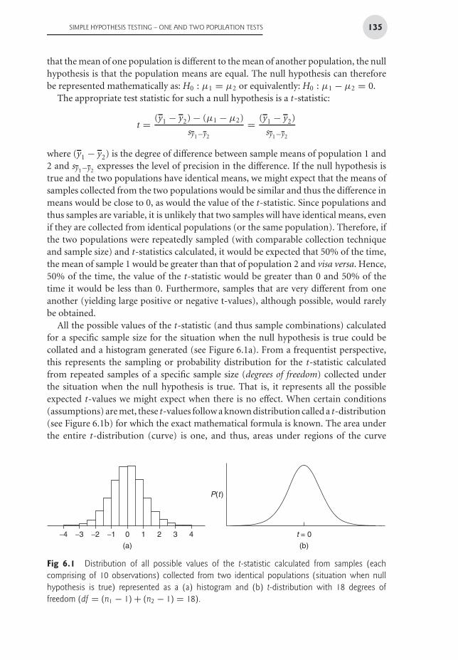
All the possible values of the t-statistic (and thus sample combinations) calculatedfor a specific sample size for the situation when the null hypothesis is true could becollated and a histogram generated (see Figure 6.1a). From a frequentist perspective,this represents the sampling or probability distribution for the t-statistic calculatedfrom repeated samples of a specific sample size (degrees of freedom) collected underthe situation when the null hypothesis is true. That is, it represents all the possibleexpected t-values we might expect when there is no effect. When certain conditions(assumptions) are met, these t-values follow a known distribution called a t-distribution(see Figure 6.1b) for which the exact mathematical formula is known. The area underthe entire t-distribution (curve) is one, and thus, areas under regions of the curve
−4 −3 −2 −1 0 4
(a)
t = 0
P(t )
(b)
1 2 3
Fig 6.1 Distribution of all possible values of the t-statistic calculated from samples (eachcomprising of 10 observations) collected from two identical populations (situation when nullhypothesis is true) represented as a (a) histogram and (b) t-distribution with 18 degrees offreedom (df = (n1 − 1) + (n2 − 1) = 18).
136 CHAPTER 6
can be calculated, which in turn represent the relative frequencies (probabilities) ofobtaining t-values in those regions. From the above example, the probability (p-value)of obtaining a t-value of greater than zero when the null hypothesis is true (populationmeans equal) is 0.5 (50%).
When real samples are collected from two populations, the null hypothesis that thetwo population means are equal is tested by calculating the real value of the t-statistic,and using an appropriate t-distribution to calculate the probability of obtaining theobserved (data) t-value or ones more extreme when the null hypothesis is true. Ifthis probability is very low (below a set critical value, typically 0.05 or 5%), it isunlikely that the sample(s) could have come from such population(s) and thus thenull hypothesis is unlikely to be true. This then provides evidence that the hypothesisis true.
Similarly, all other forms of hypothesis testing follow the same principal. Thevalue of a test statistic that has been calculated from collected data is comparedto the appropriate probability distribution for that statistic. If the probability ofobtaining the observed value of the test statistic (or ones more extreme) when the nullhypothesis is true is less than a predefined critical value, the null hypothesis is rejected,otherwise it is not rejected.
Note that the probability distributions of test statistics are strictly defined under aspecific set of conditions. For example, the t-distribution is calculated for theoreticalpopulations that are exactly normal (see chapter 3) and of identical variability. Thefurther the actual populations (and thus samples) deviate from these ideal conditions,the less reliably the theoretical probability distributions will approximate the actualdistribution of possible values of the test statistic, and thus, the less reliable the resultinghypothesis test.
6.2 One- and two-tailed tests
Two-tailed tests are any test used to test a null hypotheses that can be rejected bylarge deviations from expected in either direction. For example, when testing the nullhypothesis that two population means are equal, the null hypothesis could be rejectedif either population was greater than the other. By contrast one-tailed tests are thosetests that are used to test more specific null hypotheses that restrict null hypothesisrejection to only outcomes in one direction. For example, we could use a one-tailedtest to test the null hypothesis that the mean of population 1 was greater or equal tothe mean of population 2. This null hypothesis would only be rejected if population2 mean was significantly greater than that of population 1.
6.3 t-tests
Single population t-tests
Single population t-tests are used to test null hypotheses that a population parameteris equal to a specific value (H0 : μ = θ , where θ is typically 0), and are thus useful
SIMPLE HYPOTHESIS TESTING – ONE AND TWO POPULATION TESTS 137
for testing coefficients of regression and correlation or for testing whether measureddifferences are equal to zero.
Two population t-tests
Two population t-tests are used to test null hypotheses that two independent popula-tions are equal with respect to some parameter (typically the mean, e.g. H0 : μ1 = μ2).The t-test formula presented in section 6.1 above is used in the original studentor pooled variances t-test. The separate variances t-test (Welch’s test), representsan improvement of the t-test in that more appropriately accomodates samples withmodestly unequal variances.
Paired samples t-tests
When observations are collected from a population in pairs such that two variablesare measured from each sampling unit, a paired t-test can be used to test the nullhypothesis that the population mean difference between paired observations is equalto zero (H0 : μd = 0). Note that this is equivalent to a single population t-test testinga null hypotheses that the population parameter is equal to the specific value of zero.
6.4 Assumptions
The theoretical t-distributions were formulated for samples collected from theoret-ical populations that are 1) normally distributed (see section 3.1.1) and 2) equallyvaried. Consequently, the theoretical t-distribution will only strictly represent thedistribution of all possible values of the t-statistic when the populations from whichreal samples are collected also conform to these conditions. Hypothesis tests thatimpose distributional assumptions are known as parametric tests. Although substantialdeviations from normality and/or homogeneity of variance reduce the reliability ofthe t-distribution and thus p-values and conclusions, t-tests are reasonably robustto violations of normality and to a lesser degree, homogeneity of variance (providedsample sizes equal).
As with most hypothesis tests, t-tests also assume 3) that each of the observationsare independent (or that pairs are independent of one another in the case of pairedt-tests). If observations are not independent, then a sample may not be an unbiasedrepresentation of the entire population, and therefore any resulting analyses couldcompletely misrepresent any biological effects.
6.5 Statistical decision and power
Recall that probability distributions are typically symmetrical, bell-shaped distribu-tions that define the relative frequencies (probabilities) of all possible outcomes andsuggest that progressively more extreme outcomes become progressively less frequentor likely. By convention however, the statistical criteria for any given hypothesis test is a
138 CHAPTER 6
watershed value typically set at 0.05 or 5%. Belying the gradational decline in probabil-ities, outcomes with a probability less than 5% are considered unlikely whereas valuesequal to or greater are considered likely. However, values less than 5% are of coursepossible and could be obtained if the samples were by chance not centered similarly tothe population(s) – that is, if the sample(s) were atypical of the population(s).
When rejecting a null hypothesis at the 5% level, we are therefore accepting thatthere is a 5% change that we are making an error (a Type I error). We are concludingthat there is an effect or trend, yet it is possible that there really there is no trend, we justhad unusual samples. Conversely, when a null hypothesis is not rejected (probabilityof 5% or greater) even though there really is a trend or effect in the population, a TypeII error has been committed. Hence, a Type II error is when you fail to detect an effectthat really occurs.
Since rejecting a null hypothesis is considered to be evidence of a hypothesis ortheory and therefore scientific advancement, the scientific community projects itselfagainst too many false rejections by keeping the statistical criteria and thus Type I errorrate low (5%). However, as Type I and Type II error rates are linked, doing so leavesthe Type II error rate (β) relatively large (approximately 20%).
The reciprocal of the Type II error rate, is called power. Power is the probability thata test will detect an effect (reject a null hypothesis, not make a Type II error) if onereally occurs. Power is proportional to the statistical criteria, and thus lowering thestatistical criteria compromises power. The conventional value of α = 0.05) representsa compromise between Type I error rate and power.
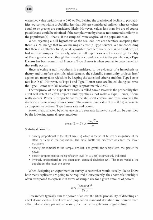
Power is also affected by other aspects of a research framework and can be describedby the following general representation:
power(1 − β) ∝ ES√
n α
σStatistical power is:
• directly proportional to the effect size (ES) which is the absolute size or magnitude of theeffect or trend in the population. The more subtle the difference or effect, the lowerthe power
• directly proportional to the sample size (n). The greater the sample size, the greater thepower
• directly proportional to the significance level (α = 0.05) as previously indicated• inversely proportional to the population standard deviation (σ ). The more variable the
population, the lower the power
When designing an experiment or survey, a researcher would usually like to knowhow many replicates are going to be required. Consequently, the above relationship isoften transposed to express it in terms of sample size for a given amount of power:
n ∝ (power σ )2
ES α
Researchers typically aim for power of at least 0.8 (80% probability of detecting aneffect if one exists). Effect size and population standard deviation are derived fromeither pilot studies, previous research, documented regulations or gut feeling.
SIMPLE HYPOTHESIS TESTING – ONE AND TWO POPULATION TESTS 139
6.6 Robust tests
There are a number of more robust (yet less powerful) alternatives to independent sam-ples t-tests and paired t-tests. The Mann-Whitney-Wilcoxon testb is a non-parametric(rank-based) equivalent of the independent samples t-test that uses the ranks of theobservations to calculate test statistics rather than the actual observations and tests thenull hypothesis that the two sampled populations have equal distributions. Similarly,the non-parametric Wilcoxon signed-rank test uses the sums of positive and negativesigned ranked differences between paired observations to test the null hypothesis thatthe two sets of observations come from the one population. While neither test dictatethat sampled populations must follow a specific distribution, the Wilcoxon signed-ranktest does assume that the population differences are symmetrically distributed aboutthe median and the Mann-Whitney test assumes that the sampled populations areequally varied (although violations of this assumption apparently have little impact).Randomization tests in which the factor levels are repeatedly shuffled so as to yield aprobability distribution for the relevant statistic (such as the t-statistic) specific to thesample data do not have any distributional assumptions. Strictly however, randomiza-tion tests examine whether the sample patterns could have occurred by chance and donot pertain to populations.
6.7 Further reading
• Theory
Fowler, J., L. Cohen, and P. Jarvis. (1998). Practical statistics for field biology. JohnWiley & Sons, England.
Hollander, M., and D. A. Wolfe. (1999). Nonparametric statistical methods, 2ndedition. John Wiley & Sons, New York.
Manly, B. F. J. (1991). Randomization and Monte Carlo methods in biology. Chapman& Hall, London.
Quinn, G. P., and K. J. Keough. (2002). Experimental design and data analysis forbiologists. Cambridge University Press, London.
Sokal, R., and F. J. Rohlf. (1997). Biometry, 3rd edition. W. H. Freeman, San Francisco.
Zar, G. H. (1999). Biostatistical methods. Prentice-Hall, New Jersey.
• Practice - R
Crawley, M. J. (2007). The R Book. John Wiley, New York.
Dalgaard, P. (2002). Introductory Statistics with R. Springer-Verlag, New York.
Maindonald, J. H., and J. Braun. (2003). Data Analysis and Graphics Using R - AnExample-based Approach. Cambridge University Press, London.
Wilcox, R. R. (2005). Introduction to Robust Estimation and Hypothesis Testing.Elsevier Academic Press.
b The Mann-Whitney U-test and the Wilcoxon two-sample test are two computationally differenttests that yield identical statistics.
140 CHAPTER 6
6.8 Key for simple hypothesis testing
1 a. Mean of single sample compared to a specific fixed value (such as a predictedpopulation mean) (one-sample t-test) . . . . . . . . . . . . . . . . . . . . . . . . . . . . . . . . . . Go to 3
b. Two samples used to compare the means of two populations . . . . . . . . . . . . . Go to 22 a. Two completely independent samples (different sampling units used for each
replicate of each condition) (independent samples t-test) . . . . . . . . . . . . . . . . . Go to 3
FACTOR DV
A .A ... ..B .B ... ..
Dataset should be constructed inlong format such that the variablesare in columns and each replicate isin is own row.
b. Two samples specifically paired (each of the sampling units measured under bothconditions) to reduce within-group variation (paired t-test) . . . . . . . . . . . . . . Go to 3
Pair FACTOR DV
1 A .2 A ... .. ..1 B .2 B ... ..
Dataset can be constructed in eitherlong format (left) such that thevariables are in columns and eachreplicate is in is own row or in wideformat (right) such that each pairof measurements has its own row.
Pair DV1 DV2
1 . .2 . .3 . .4 . .5 . ... .. ..
3 a. Check parametric assumptions
• Normality of the response variable at both level of the categorical variable -boxplots
• one-sample t-test
> boxplot(DV, dataset)
• two-sample t-test
> boxplot(DV ~ Factor, dataset)
• paired t-test
> with(dataset, boxplot(DV1 - DV2))
> diffs <- with(dataset, DV[FACTOR == "A"]
+ - DV[FACTOR == "B"])
> boxplot(diffs)
where DV and Factor are response and factor variables respectively in the datasetdata frame. DV1 and DV2 represent the paired responses for group one and twoof a paired t-test. Note, paired t-test data is traditionally setup in wide format(see section 2.7.6)
SIMPLE HYPOTHESIS TESTING – ONE AND TWO POPULATION TESTS 141
• Homogeneity of variance (two-sample t-tests only) - boxplots (as above) andscatterplot of mean vs variance
> boxplot(DV ~ Factor, dataset)
where DV and FACTOR are response and factor variables respectively in the datasetdata frame
Example 6A: Pooled variances, student t-testWard and Quinn (1988) investigated differences in the fecundity (as measured by eggproduction) of a predatory intertidal gastropod (Lepsiella vinosa) in two different intertidalzones (mussel zone and the higher littorinid zone) (Box 3.2 of Quinn and Keough (2002)).
Step 1 - Import (section 2.3) the Ward and Quinn (1988) data set.
Step 2 (Key 6.3) - Assess assumptions of normality and homogeneity of variance for the nullhypothesis that the population mean egg production is the same for both littorinid and musselzone Lepsiella.
> boxplot(EGGS ~ ZONE, ward)
Littor Mussel
610
1214
1618
8
SIMPLE HYPOTHESIS TESTING – ONE AND TWO POPULATION TESTS 143
Conclusions - There was no evidence of non-normality (boxplots not grossly asymmetrical)or unequal variance (boxplots very similar size and variances very similar). Hence, the simple,studentized (pooled variances) t-test is likely to be reliable.
Step 3 (Key 6.4b) - Perform a pooled variances t-test to test the null hypothesis thatthe population mean egg production is the same for both littorinid and mussel zoneLepsiella.
> t.test(EGGS ~ ZONE, ward, var.equal = T)
Two Sample t-test
data: EGGS by ZONE
t = -5.3899, df = 77, p-value = 7.457e-07
alternative hypothesis: true difference in means is not equal to 0
95 percent confidence interval:
-3.635110 -1.673770
sample estimates:
mean in group Littor mean in group Mussel
8.702703 11.357143
Conclusions - Reject the null hypothesis. Egg production by predatory gastropods (Lepsiellavinosa was significantly greater (t77 = −5.39, P < 0.001) in mussel zones than littorinid zoneson rocky intertidal shores.
> mtext(2, text = "Mean number of egg capsules per capsule",
+ line = 3, cex = 1)
> mtext(1, text = "Zone", line = 3, cex = 1)
> box(bty = "l")
144 CHAPTER 6
8
9
10
11
12
Littorinid Mussel
Mea
n nu
mbe
r of
egg
cap
sule
s pe
r ca
psul
e
Zone
Example 6B: Separate variances, Welch’s t-testFurness and Bryant (1996) measured the metabolic rates of eight male and six femalebreeding northern fulmars and were interesting in testing the null hypothesis that therewas no difference in metabolic rate between the sexes (Box 3.2 of Quinn and Keough(2002)).
Step 1 - Import (section 2.3) the Furness and Bryant (1996) data set.
Step 2 (Key 6.3) - Assess assumptions of normality and homogeneity of variance for the nullhypothesis that the population mean metabolic rate is the same for male and female breedingnorthern fulmars.
SIMPLE HYPOTHESIS TESTING – ONE AND TWO POPULATION TESTS 145
Conclusions - Whilst there is no evidence of non-normality (boxplots not grossly asymmetri-cal), variances are a little unequal (although perhaps not grossly unequal - one of the boxplotsis not more than three times smaller than the other). Hence, a separate variances t-test is moreappropriate than a pooled variances t-test.
Step 3 (Key 6.4b) - Perform a separate variances (Welch’s) t-test to test the null hypothesisthat the population mean metabolic rate is the same for both male and female breeding northernfulmars.
> t.test(METRATE ~ SEX, furness, var.equal = F)
Welch Two Sample t-test
data: METRATE by SEX
t = -0.7732, df = 10.468, p-value = 0.4565
alternative hypothesis: true difference in means is not equal to 0
95 percent confidence interval:
-1075.3208 518.8042
sample estimates:
mean in group Female mean in group Male
1285.517 1563.775
Conclusions - Do not reject the null hypothesis. Metabolic rate of male breeding northernfulmars was not found to differ significantly (t = −0.773, df = 10.468, P = 0.457) from thatof females.
Example 6C: Paired t-testTo investigate the effects of lighting conditions on the orb-spinning spider webs Elgar et al.(1996) measured the horizontal (width) and vertical (height) dimensions of the webs madeby 17 spiders under light and dim conditions. Accepting that the webs of individual spidersvary considerably, Elgar et al. (1996) employed a paired design in which each individualspider effectively acts as its own control. A paired t-test performs a one sample t-test onthe differences between dimensions under light and dim conditions (Box 3.3 of Quinn andKeough (2002)).
Step 1 - Import (section 2.3) the Elgar et al. (1996) data set.
Note the format of this data set. Rather than organizing the data into the usual long formatin which variables are represented in columns and rows represent individual replicates, thesedata have been organized in wide format. Wide format is often used for data containingrepeated measures from individual or other sampling units. Whilst, this is not necessary (aspaired t-tests can be performed on long format data), traditionally it did allow more compactdata management as well as making it easier to calculate the differences between repeatedmeasurements on each individual.
Step 2 (Key 6.3) - Assess whether the differences in web width (and height) in light and dimlight conditions are normally distributed.
146 CHAPTER 6
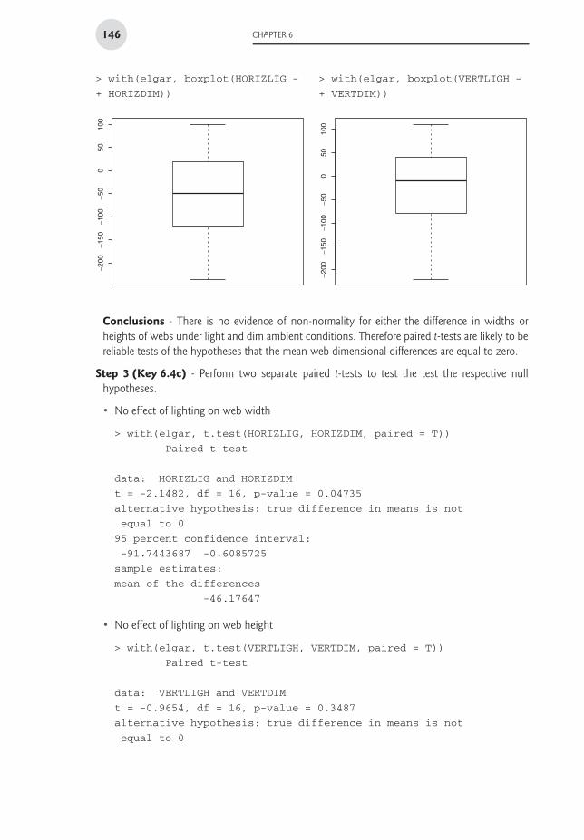
> with(elgar, boxplot(HORIZLIG -
+ HORIZDIM))
> with(elgar, boxplot(VERTLIGH -
+ VERTDIM))−2
00−1
50−1
00−5
00
5010
0
−200
−150
−100
−50
050
100
Conclusions - There is no evidence of non-normality for either the difference in widths orheights of webs under light and dim ambient conditions. Therefore paired t-tests are likely to bereliable tests of the hypotheses that the mean web dimensional differences are equal to zero.
Step 3 (Key 6.4c) - Perform two separate paired t-tests to test the test the respective nullhypotheses.
alternative hypothesis: true difference in means is not
equal to 0
SIMPLE HYPOTHESIS TESTING – ONE AND TWO POPULATION TESTS 147
95 percent confidence interval:
-65.79532 24.61885
sample estimates:
mean of the differences
-20.58824
Conclusions - Orb-spinning spider webs were found to be significantly wider (t = 2.148,df = 16, P = 0.047) under dim lighting conditions than light conditions, yet were not foundto differ (t = 0.965, df = 16, P = 0.349) in height.
Example 6D: Non-parametric Mann-Whitney-Wilcoxon signed rank testSokal and Rohlf (1997) presented a dataset comprising the lengths of cheliceral bases(in μm) from two samples of chigger (Trombicula lipovskyi) nymphs. These data were usedto illustrate two equivalent tests (Mann-Whitney U-test and Wilcoxon two-sample test) oflocation equality (Box 13.7 of Sokal and Rohlf (1997)).
Step 2 (Key 6.3) - Assess assumptions of normality and homogeneity of variance for the nullhypothesis that the population mean metabolic rate is the same for male and female breedingnorthern fulmars.
Conclusions - Whilst there is no evidence of unequal variance, there is some (possible)evidence of non-normality (boxplots slightly asymmetrical). These data will therefore beanalysed using a non-parametric Mann-Whitney-Wilcoxon signed rank test.
148 CHAPTER 6
Step 3 (Key 6.8b) - Perform a Mann-Whitney Wilcoxon test to investigate the null hypothesisthat the mean length of cheliceral bases is the same for the two samples of nymphs of chigger(Trombicular lipovskyi).
> wilcox.test(LENGTH ~ SAMPLE, nymphs)
Wilcoxon rank sum test with continuity correction
data: LENGTH by SAMPLE
W = 123.5, p-value = 0.02320
alternative hypothesis: true location shift is not equal to 0
Conclusions - Reject the null hypothesis. The length of the cheliceral base is significantlylonger in nymphs from sample 1 (W = 123.5, df = 24, P = 0.023) than those from sample 2.
Example 6E: Randomization t-testPowell and Russell (1984, 1985) investigated differences in beetle consumption betweentwo size classes of eastern horned lizard (Phrynosoma douglassi brevirostre) representedrespectively by adult females in the larger class and adult male and yearling females in thesmaller class (Example 4.1 from Manly, 1991).
Step 1 - Import (section 2.3) the Powell and Russell (1984, 1985) beetle data set.
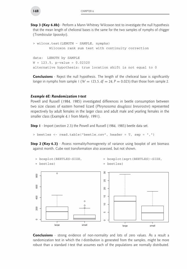
Step 2 (Key 6.3) - Assess normality/homogeneity of variance using boxplot of ant biomassagainst month. Cube root transformation also assessed, but not shown.
> boxplot(BEETLES~SIZE,
+ beetles)
large small
020
040
060
080
0
> boxplot(sqrt(BEETLES)~SIZE,
+ beetles)
large small
010
1520
2530
5
Conclusions - strong evidence of non-normality and lots of zero values. As a result arandomization test in which the t-distribution is generated from the samples, might be morerobust than a standard t-test that assumes each of the populations are normally distributed.
SIMPLE HYPOTHESIS TESTING – ONE AND TWO POPULATION TESTS 149
Furthermore, the observations need not be independent, provided we are willing to concede thatwe are no longer testing hypotheses about populations (rather, we are estimating the probabilityof obtaining the observed differences in beetle consumption between the size classes just bychance).
Step 3 (Key 6.7b) - define the statistic to use in the randomization test – in this case thet-statistic (without replacement).
> stat <- function(data, indices) {
+ t.test <- t.test(BEETLES ~ SIZE, data)$stat
+ t.test
+ }
Step 4 (Key 6.7b) - define how the data should be randomized – randomly reorder the whichsize class that each observation belonged to.
> rand.gen <- function(data, mle) {
+ out <- data
+ out$SIZE <- sample(out$SIZE, replace = F)
+ out
+ }
Step 5 (Key 6.7b) - call a bootstrapping procedure to randomize 5000 times (this can takesome time).
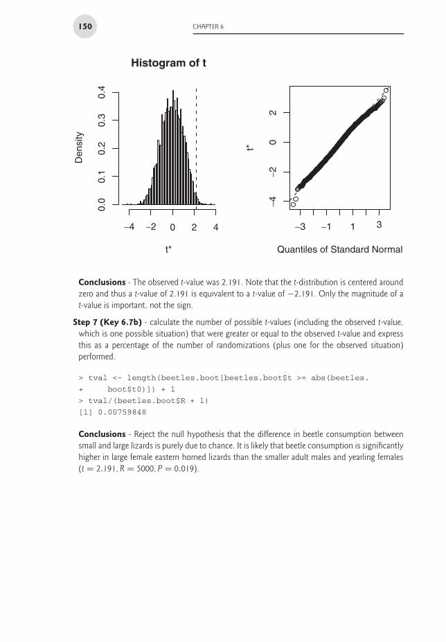
2Conclusions - The observed t-value was 2.191. Note that the t-distribution is centered aroundzero and thus a t-value of 2.191 is equivalent to a t-value of −2.191. Only the magnitude of at-value is important, not the sign.
Step 7 (Key 6.7b) - calculate the number of possible t-values (including the observed t-value,which is one possible situation) that were greater or equal to the observed t-value and expressthis as a percentage of the number of randomizations (plus one for the observed situation)performed.
Conclusions - Reject the null hypothesis that the difference in beetle consumption betweensmall and large lizards is purely due to chance. It is likely that beetle consumption is significantlyhigher in large female eastern horned lizards than the smaller adult males and yearling females(t = 2.191, R = 5000, P = 0.019).