207
Biostatistics Unit 7 – Hypothesis Testing
| Date post: | 29-Dec-2015 |
| Category: |
Documents |
| Upload: | loraine-eaton |
| View: | 229 times |
| Download: | 1 times |

Biostatistics
Unit 7 – Hypothesis Testing

Testing Hypotheses
Hypothesis testing and estimation are used to reach conclusions about a population by examining a sample of that population. Hypothesis testing is widely used in medicine, dentistry, health care, biology and other fields as a means to draw conclusions about the nature of populations.
(continued)

Hypothesis testing
Hypothesis testing is to provide information in helping to make decisions. The administrative decision usually depends a test between two hypotheses. Decisions are based on the outcome.

Definitions
Hypothesis: A hypothesis is a statement about one or more populations. There are research hypotheses and statistical hypotheses.

Definitions
Research hypothesis: A research hypothesis is the supposition or conjecture that motivates the research. It may be proposed after numerous repeated observation. Research hypotheses lead directly to statistical hypotheses.

Definitions
Statistical hypotheses: Statistical hypotheses are stated in such a way that they may be evaluated by appropriate statistical techniques. There are two statistical hypotheses involved in hypothesis testing.
(continued)

Definitions
is the null hypothesis or the hypothesis of no
difference.
(otherwise known as ) is the alternative
hypothesis or what we will believe is true if we reject the null hypothesis.

Rules for testing hypotheses
1. Your expected conclusion, or what you hope to conclude as a result of the experiment should be placed in the alternative hypothesis.
2. The null hypothesis should contain an expression of equality, either =, or .
3. The null hypothesis is the hypothesis that will be tested.
(continued)

Rules for testing hypotheses
4. The null and alternative hypotheses are complementary. This means that the two alternatives together exhaust all possibilities of the values that the hypothesized parameter can assume.
Note: Neither hypothesis testing nor statistical inference proves the hypothesis. It only indicates whether the hypothesis is supported by the data or not.

Stating statistical hypotheses
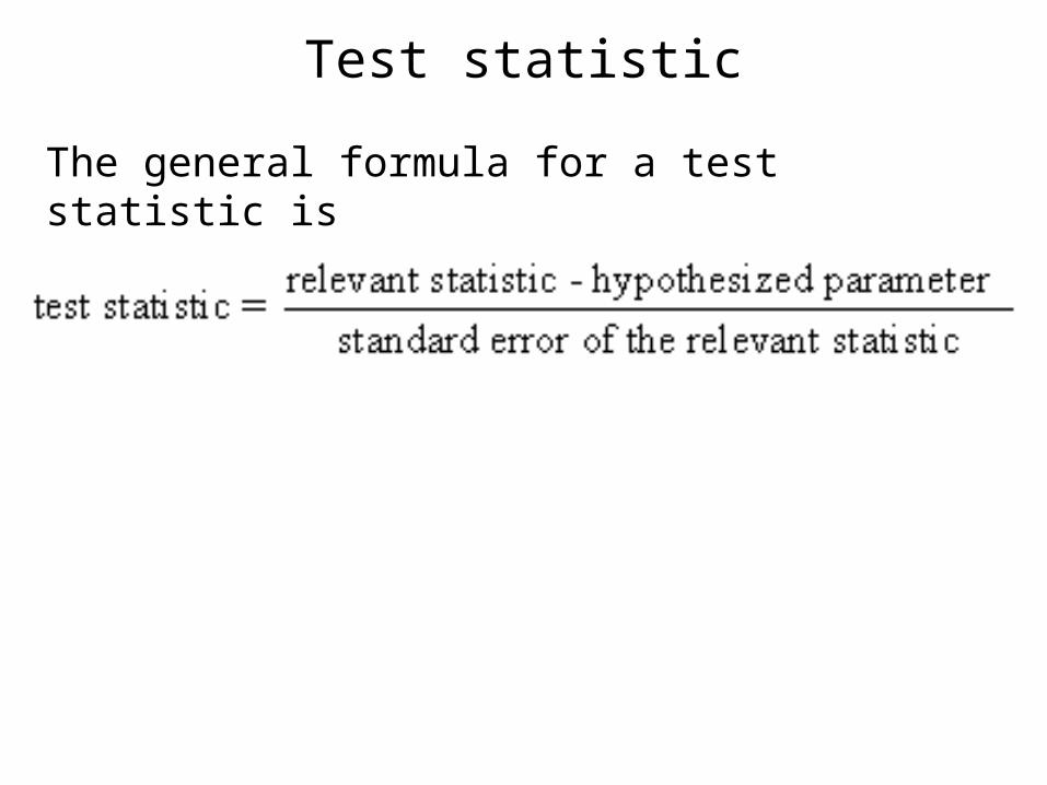
Test statistic
The general formula for a test statistic is

Example of test statistic
sample mean
hypothesized parameter— population mean
standard error of which is the relevant statistic
This all depends on the assumptions being correct.
Level of significance
The level of significance, , is a probability and is, in reality, the probability of rejecting a true null hypothesis. For example, with 95% confidence intervals, = .05 meaning that there is a 5% chance that the parameter does not fall within the 95% confidence region. This creates an error and leads to a false conclusion.

Significance and errors
When the computed value of the test statistic falls in the rejection region it is said to be significant. We select a small value of such as .10, .05 or .01 to make the probability of rejecting a true null hypothesis small.

Types of errors
•When a true null hypothesis is rejected, it causes a Type I error whose probability is .•When a false null hypothesis is not rejected, it causes a Type II error whose probability is designated by .•A Type I error is considered to be more serious than a Type II error.

Table of error conditions

Risk management
Since rejecting a null hypothesis has a chance of committing a type I error, we make small by selecting an appropriate confidence interval. Generally, we do not control , even though it is generally greater than . However, when failing to reject a null hypothesis, the risk of error is unknown.
Procedure for hypothesis testing
In science, as in other disciplines, certain methods and procedures are used for performing experiments and reporting results. A research report in the biological sciences generally has five sections.

Procedure for hypothesis testing
I. Introduction The introduction contains a statement of the problem to be solved, a summary of what is being done, a discussion of work done before and other basic background for the paper.
Procedure for hypothesis testing
II. Materials and methods
The biological, chemical and physical materials used in the experiments are described. The procedures used are given or referenced so that the reader may repeat the experiments if s/he so desires.
Procedure for hypothesis testing
III. Results
A section dealing with the outcomes of the experiments. The results are reported and sometimes explained in this section. Other explanations are placed in the discussion section.

Procedure for hypothesis testing
IV. Discussion
The results are explained in terms of their relationship to the solution of the problem under study and their meaning.

Procedure for hypothesis testing
V. Conclusions
Appropriate conclusions are drawn from the information obtained as a result of performing the experiments.

Procedure for hypothesis testing
This method can be modified for use in biostatistics. The materials and procedures used in biostatistics can be made to fit into these five categories. Alternatively, we will use an approach that is similar in structure but contains seven sections.

Procedure for hypothesis testing
a. Givenb. Assumptionsc. Hypothesesd. Statistical teste. Calculations
f. Discussiong. Conclusions

Explanation of procedure
a. Given
This section contains introductory material such as the measurements or counts given in the statement of the problem. It should contain enough information so as to solve the problem without further information

Explanation of procedure
b. Assumptions
This is another set of introductory material that is necessary for a correct solution of the problem. In biostatistics, problems are solved and conclusions drawn based on certain assumptions being true. If they are not true the results may be invalid.

Explanation of procedure
c. Hypotheses
The specific hypotheses being tested are written H0 : the null hypothesis HA : the alternative hypothesis

Explanation of procedure
d. Test statistic
In this section, several items are necessary.
First, decide on the test statistic that will be used. for example z or t. It must be possible to compute the test statistic from the data of the sample. How it is set up depends on how the hypotheses are stated.

Explanation of procedure
Second, the distribution of the test statistic must be known. For example, the z statistic is distributed as the standard normal distribution whereas the t statistic is distributed following Student's t distribution.

Explanation of procedure
Third, the criteria for making the decision are required. It is best to draw an actual distribution with rejection and non-rejection regions. The values of the test statistic that mark the regions should be calculated in advance so that when the problem is solved, the resulting figure can be compared immediately.

Explanation of procedure
e. Calculations
The test statistic is calculated using the data given in the problem. The result is compared with the previously specified rejection and non-rejection regions.

Explanation of procedure
f. Discussion
A statistical decision is made on whether to reject the null hypothesis or not.

Explanation of procedure
g. Conclusion
After the statistical decision is made, conclusions are drawn. What is reported depends on the statistical decision made in the Discussion section.
If H0 is rejected we conclude that HA is true. This conclusion can be stated as written.

Explanation of procedure
If H0 is not rejected , then we conclude that H0 may be true. Caution is required when reporting this outcome. One should not say "H0 is true," because there is always a chance of making a Type II error. This would mean that a false null hypothesis was not rejected. It is better to say, "H0 may be true." in this case.

Purpose of hypothesis testing
Hypothesis testing is to provide information in helping to make decisions. The administrative decision usually depends on the null hypothesis. If the null hypothesis is rejected, usually the administrative decision will follow the alternative hypothesis.
(continued)
Purpose of hypothesis testing
It is important to remember never to base a decision solely on the outcome of only one test. Statistical testing can be used to provide additional support for decisions based on other relevant information.

Topics
Hypothesis Testing of a Single Population Mean
Hypothesis Testing of the Difference Between Two Population Means
Hypothesis Testing of a Single Population Proportion
Hypothesis Testing of the Difference Between Two Population Proportions
Hypothesis Testing of a Single Population Variance
Hypothesis Testing of the Ratio of Two Population Variances

A) Hypothesis testing of a single population mean
A hypothesis about a population mean can be tested when sampling is from any of the following.• A normally distributed population--variances known

Hypothesis testing of a single population mean
• A normally distributed population--variances unknown

Hypothesis testing of a single population mean
• A population that is not normally distributed (assuming n 30; the central limit theorem applies)
p values
A p value is a probability that the result is as extreme or more extreme than the observed value if the null hypothesis is true. If the p value is less than or equal to , we reject the null hypothesis, otherwise we do not reject the null hypothesis.

One tail and two tail tests
In a one tail test, the rejection region is at one end of the distribution or the other. In a two tail test, the rejection region is split between the two tails. Which one is used depends on the way the null hypothesis is written.
Confidence intervals
A confidence interval can be used to test hypotheses. For example, if the null hypothesis is: H0: = 30, a 95% confidence interval can be
constructed. If 30 were within the confidence interval, we could conclude that the null hypothesis is not rejected at that level of significance.

Procedure
The procedure of seven steps is followed for hypothesis testing. It is very important to observe several items.• Avoid rounding numbers off until the very end of the problem. • Pay strict attention to details.• Be very careful with regard to the way things are worded.• Write down all the steps and do not take short cuts.

Sampling from a normally distributed population--variance known
•Example 7.2.1
A simple random sample of 10 people from a certain population has a mean age of 27. Can we conclude that the mean age of the population is not 30? The variance is known to be 20. Let = .05.

Solution
a. Data
n = 10 = 20
= 27 = .05

Solution
b. Assumptions• simple random sample• normally distributed population
Solution
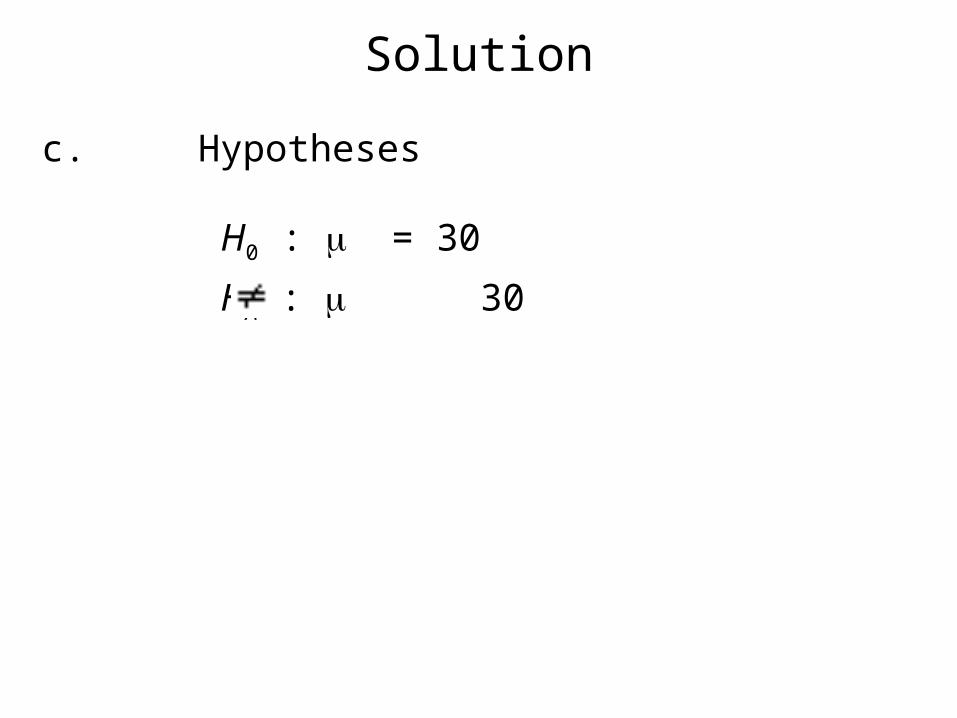
c. Hypotheses
H0 : = 30
HA : 30
Solution
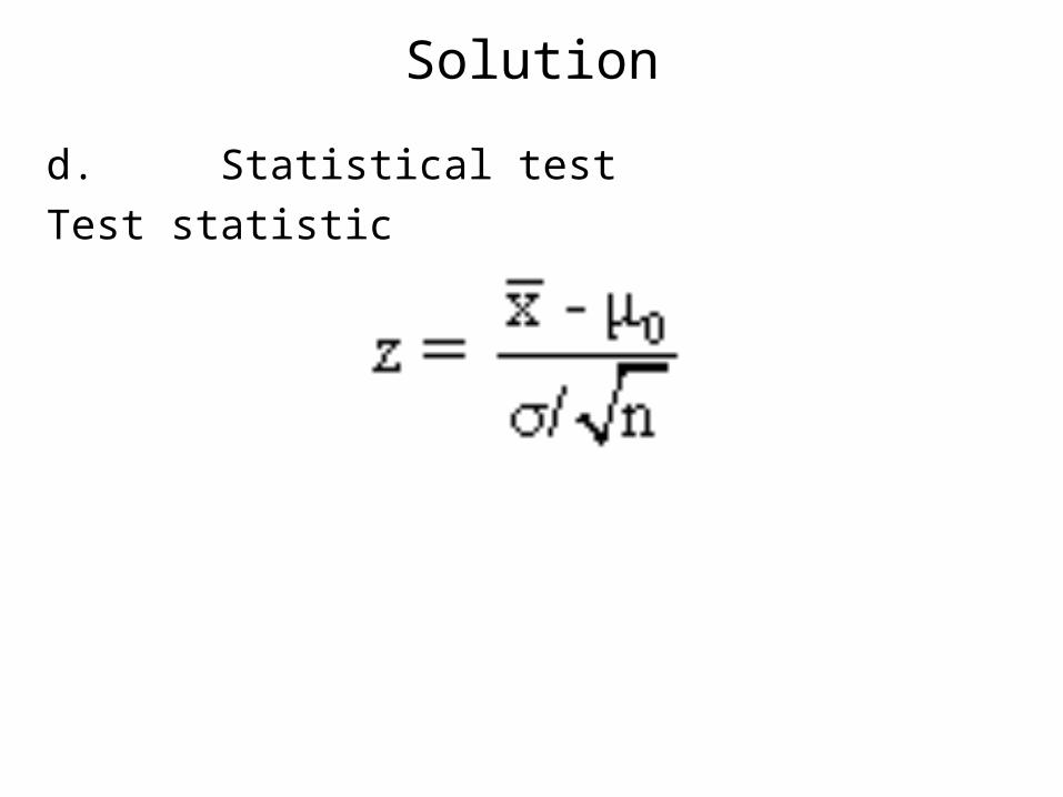
d. Statistical test
Test statistic

Solution
d. Statistical test
Distribution of test statistic
If the assumptions are correct and H0 is true, the test statistic follows the standard normal distribution.
Solution
d. Statistical test
Decision criteria
Reject H0 if the z value falls in the rejection region. Fail to reject H0 if it falls in the nonrejection region.
Solution
d. Statistical test -- Decision criteria

Solution
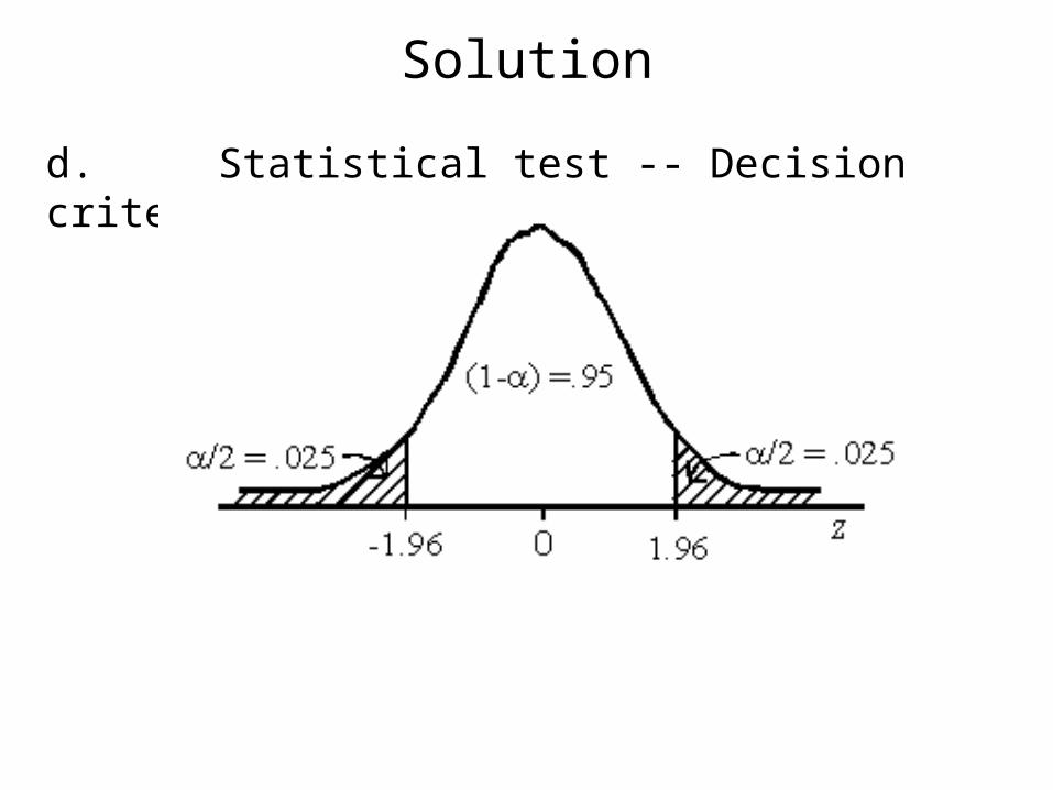
d. Statistical test
Decision criteria
Because of the structure of H0 it is a two tail test. Therefore, reject H0 if z -1.96 or z 1.96.

Solution
e. Calculations
Solution
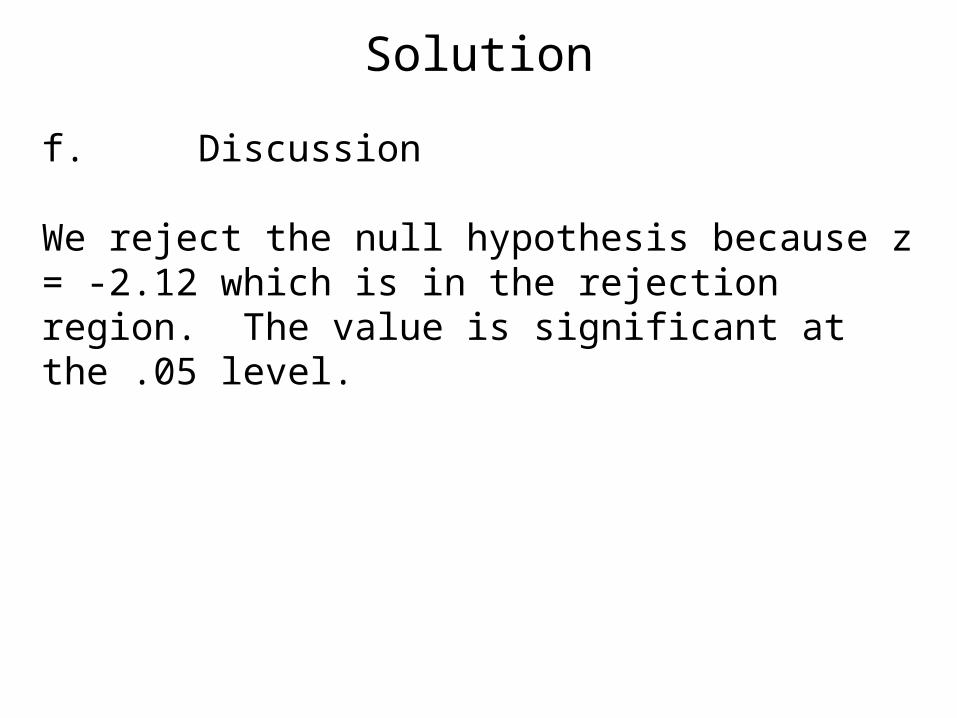
f. Discussion
We reject the null hypothesis because z = -2.12 which is in the rejection region. The value is significant at the .05 level.

Solution
g. Conclusions
We conclude that is not 30.
p = .0340
(continued)

Solution
g. Conclusions
A z value of -2.12 corresponds to an area of .0170. Since there are two parts to the rejection region in a two tail test, the p value is twice this which is .0340.

Confidence interval

Solution
Same example as a one tail test.Example 7.2.1 (reprise)
A simple random sample of 10 people from a certain population has a mean age of 27. Can we conclude that the mean age of the population is less than 30? The variance is known to be 20. Let = .05.

Solution
a. Given
n = 10 = 20
= 27 = .05

Solution
b. Assumptions• simple random sample• normally distributed population

Solution
c. Hypotheses
H0: 30
HA: < 30

Solution
d. Statistical test

Solution
d. Statistical test
Distribution
If the assumptions are correct and H0 is true, the test statistic follows the standard normal distribution. Therefore, we calculate a z score and use it to test the hypothesis.

Solution
d. Statistical test
Decision criteria
Reject H0 if the z value falls in the rejection region. Fail to reject H0 if it falls in the nonrejection region.

Solution
d. Statistical test -- Decision criteria

Solution
d. Statistical test
Decision criteria
With = .05 and the inequality we have the entire rejection region at the left. The critical value will be
z = -1.645. Reject H0 if z < -1.645.

Solution
e. Calculations

Solution
f. Discussion
We reject the null hypothesis because
-2.12 < -1.645.
Solution
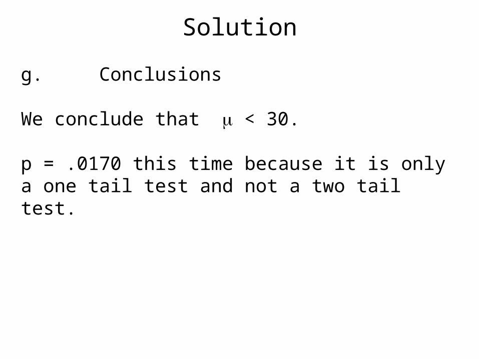
g. Conclusions
We conclude that < 30.
p = .0170 this time because it is only a one tail test and not a two tail test.

Sampling is from a normally distributed population--variance unknown.
Example 7.2.3 Body mass index
A simple random sample of 14 people from a certain population gives body mass indices as shown in Table 7.2.1. Can we conclude that the BMI is not 35? Let = .05.


Solution
a. Givenn = 14
s = 10.63918736 = 30.5
= .05

Solution
b. Assumptions
• simple random sample
• population of similar subjects
• normally distributed

Solution
c. Hypotheses
H0: = 35 HA: 35

Solution
d. Test statistic

Solution
d. Distribution
If the assumptions are correct and H0 is true, the test statistic follows Student's t distribution with 13 degrees of freedom.

Solution
d. Decision criteriaWe have a two tail test. With = .05 it means that each tail is 0.025. The critical t values with 13 df are -2.1604 and 2.1604.
We reject H0 if the t -2.1604 or t 2.1604.

decision criteria

Solution
e. Calculation of test statistic

Solution
f. Discussion
Do not reject the null hypothesis because -1.58 is not in the rejection region.

Solution
g. Conclusions
Based on the data of the sample, it is possible that
= 35. The value of p = .1375

Sampling is from a population that is not normally distributed
Example 7.2.4
Maximum oxygen uptake data
Can we conclude that > 30?Let = .05.

Solution
a. Given
n = 242 s = 12.14 = 33.3 = .05

Solution
b. Assumptions• simple random sample• population is similar to those subjects in the sample
(cannot assume normal distribution)

Solution
c. Hypotheses
H0: 30
HA: > 30

Solution
d. Test statistic

Solution
Distribution
By virtue of the Central Limit Theorem, the test statistic is approximately normally distributed with
= 0 if H0 is true.
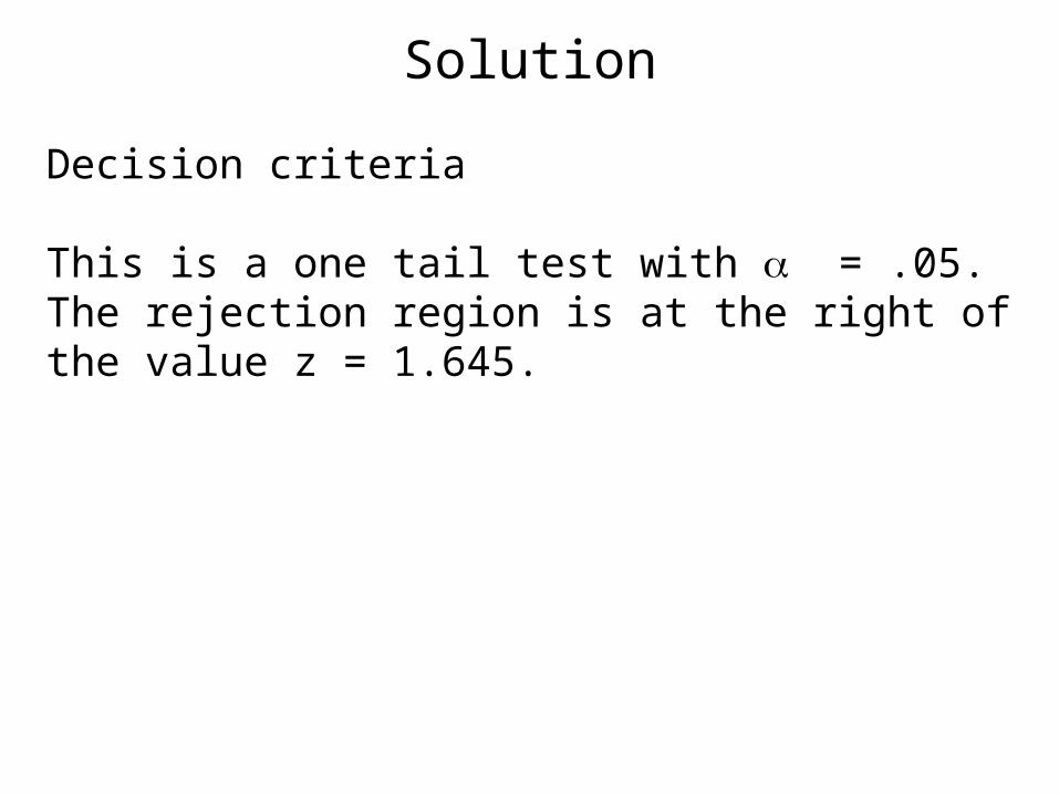
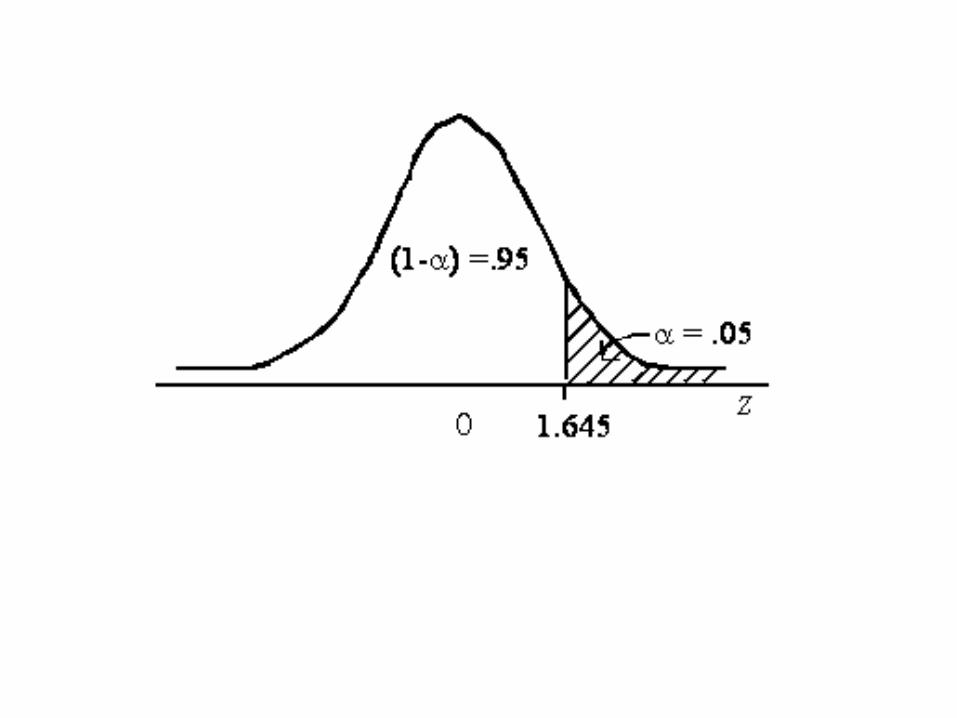
Solution
Decision criteria This is a one tail test with = .05. The rejection region is at the right of the value z = 1.645.

Solution
e. Calculations

Solution
f. Discussion
Reject H0 because 4.23 > 1.645.

Solution
g. Conclusion
The maximum oxygen uptake for the sampled population is greater than 30.The p value < .001 because 4.23 is off the chart (p(3.89) < .001). Actual value p=1.17 x 10⁻⁵ (.0000117)

B) Hypothesis testing of the difference between two population means
This is a two sample z test which is used to determine if two population means are equal or unequal. There are three possibilities for formulating hypotheses.
(continued)
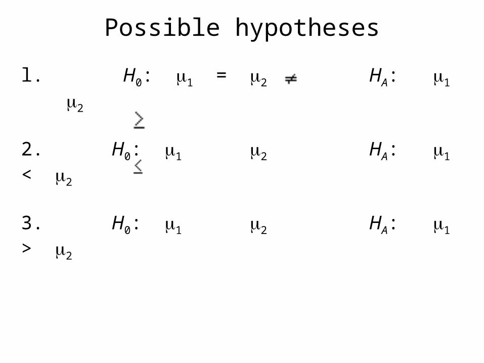
Possible hypotheses
l. H0: 1 = 2 HA: 1 2
2. H0: 1 2 HA: 1 < 2
3. H0: 1 2 HA: 1 > 2

Procedure
The same procedure is used in three different situations

Sampling is from normally distributed populations with known variances

Sampling from normally distributed populations where population variances are unknown
population variances equal This is with t distributed as Student's t distribution with n1 + n2 - 2 degrees of freedom and a pooled variance.
(continued)

Sampling from normally distributed populations where population variances are unknown
population variances equal--distribution

Sampling from normally distributed populations where population variances are unknown
population variances equal—pooled variance

population variances unequal
When population variances are unequal, a distribution of t' is used in a manner similar to calculations of confidence intervals in similar circumstances.
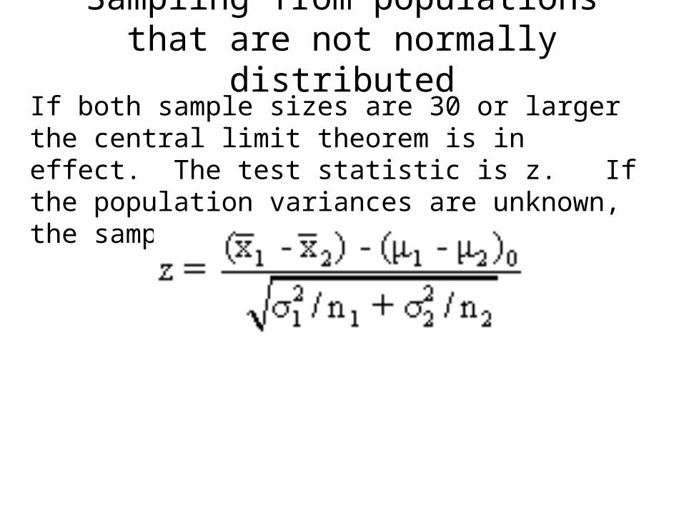
Sampling from populations that are not normally distributed
If both sample sizes are 30 or larger the central limit theorem is in effect. The test statistic is z. If the population variances are unknown, the sample variances are used.

Sampling from normally distributed populations with population variances known
Example 7.3.1
Serum uric acid levels: Is there a difference between the means between individuals with Down's syndrome and normal individuals?

Solution
a. Given
= 4.5 n1 = 12 12 = 1
= 3.4 n2 = 15 22 = 1.5 = .05

Solution
b. Assumptions• two independent random samples• each drawn from a normally distributed population

Solution
c. Hypotheses
H0: 1 = 2
HA: 1 2
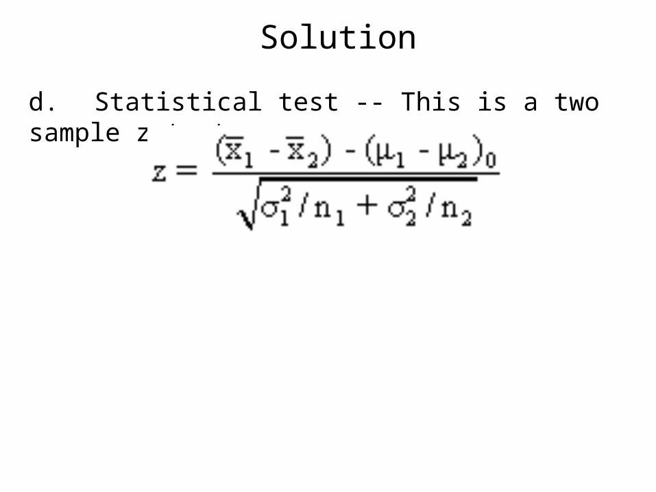
Solution
d. Statistical test -- This is a two sample z test.

Solution
Distribution
If the assumptions are correct and H0 is true, the test statistic is distributed as the normal distribution.

Solution
Decision criteria
With = .05, the critical values of z are -1.96 and +1.96. We reject H0 if z < -1.96 or z > +1.96.

Solution
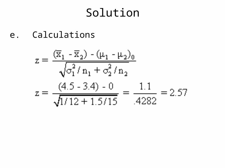
Solution
e. Calculations

Solution
f. Discussion
Reject H0 because 2.57 > 1.96.

Solution
g. Conclusion
From these data, it can be concluded that the population means are not equal. A 95% confidence interval would give the same conclusion.
p = .0102.

Sampling from normally distributed populations with unknown variances
With equal population variances, we can obtain a pooled value from the sample variances.
(continued)

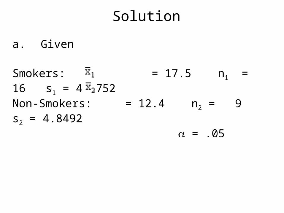
Example 7.3.2 -- Lung destructive index
We wish to know if we may conclude, at the 95% confidence level, that smokers, in general, have greater lung damage than do non-smokers.
Solution
a. Given
Smokers: = 17.5 n1 = 16 s1 = 4.4752Non-Smokers: = 12.4 n2 = 9 s2 = 4.8492 = .05
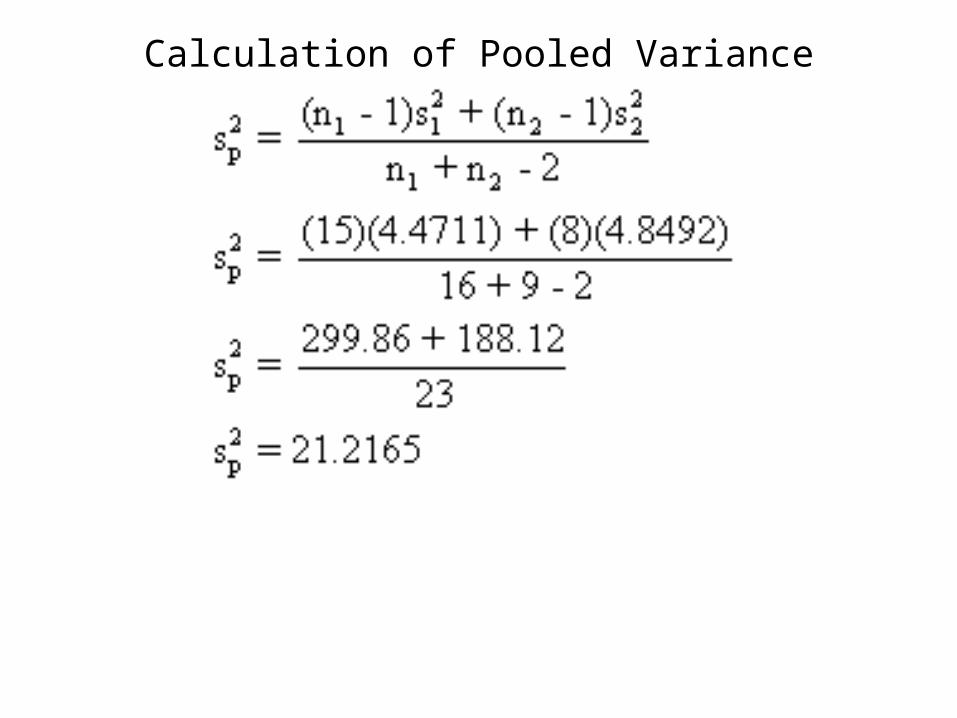
Calculation of Pooled Variance
Solution
b. Assumptions• independent random samples• normal distribution of the populations• population variances are equal

Solution
(3) Hypotheses
H0: 1 2
HA: 1 > 2

Solution
d. Statistical test -- Test statistic

Distribution of test statistic
If the assumptions are met and H0 is true, the test statistic is distributed as Student's t distribution with 23 degrees of freedom.

Decision criteria
With = .05 and df = 23, the critical value of t is 1.7139. We reject H0 if t > 1.7139.

Solution
e. Calculations

Solution
f. Discussion
Reject H0 because 2.6563 > 1.7139.
Solution
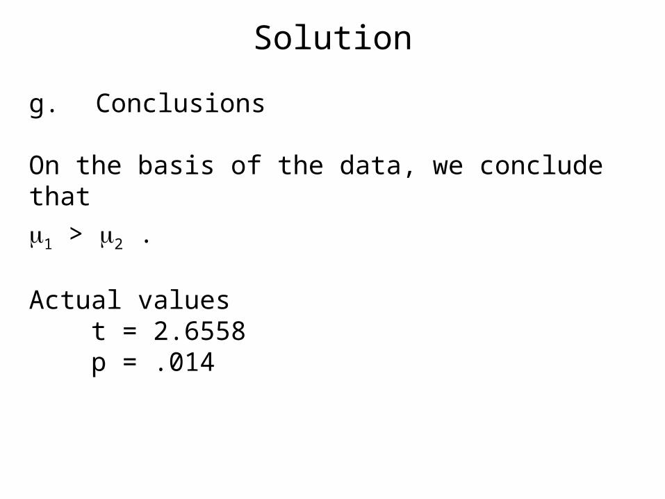
g. Conclusions
On the basis of the data, we conclude that
1 > 2 .
Actual values t = 2.6558 p = .014

Sampling from populations that are not normally distributed -- Example 7.3.4
These data were obtained in a study comparing persons with disabilities with persons without disabilities. A scale known as the Barriers to Health Promotion Activities for Disabled Persons (BHADP) Scale gave the data. We wish to know if we may conclude, at the 99% confidence level, that persons with disabilities score higher than persons without disabilities.

Solution
a. Given
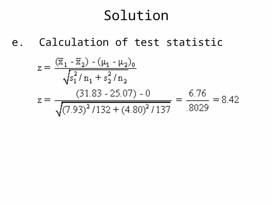
Disabled: = 31.83 n1 = 132 s1 = 7.93Nondisabled: = 25.07 n2 = 137 s2 = 4.80 = .01
Solution
b. Assumptions
• independent random samples

Solution
c. Hypotheses
H0: 1 2
HA: 1 > 2

Solution
d. Statistical test -- Test statistic
Because of the large samples, the central limit theorem permits calculation of the z score as opposed to using t. The z score is calculated using the given sample standard deviations.
Solution
Distribution
If the assumptions are correct and H0 is true, the test statistic is approximately normally distributed

Solution
Decision criteria
With = .01 and a one tail test, the critical value of z is 2.33. We reject H0 if z > 2.33.
Solution
e. Calculation of test statistic

Solution
f. Discussion
Reject H0 because 8.42 > 2.33.

Solution
g. Conclusions
On the basis of these data, the average persons with disabilities score higher on the BHADP test than do the nondisabled persons.
Actual values z = 8.42 p = 1.91 x 10⁻¹⁷
Paired comparisons
Sometimes data come from nonindependent samples. An example might be testing "before and after" of cosmetics or consumer products. We could use a single random sample and do "before and after" tests on each person.
(continued)

Paired comparisons
A hypothesis test based on these data would be called a paired comparisons test. Since the observations come in pairs, we can study the difference, d, between the samples. The difference between each pair of measurements is called di.

Test statistic
With a population of n pairs of measurements, forming a simple random sample from a normally distributed population, the mean of the difference, d, is tested using the following implementation of t.
(continued)


Example 7.4.1
Very-low-calorie diet (VLCD) Treatment• Table gives B (before) and A (after) treatment data for obese female patients in a weight-loss program.
• We calculate di = A-B for each pair of data resulting in negative values meaning that the participants lost weight.
(continued)

Example 7.4.1
We wish to know if we may conclude, at the 95% confidence level, that the treatment is effective in causing weight reduction in these people.

Data table

Solution
a. Given
A -> L1 B -> L2
di = A – B (L1 – L2 -> L3)
n = 9 = .05

Solution
b. Assumptions• the observed differences are a simple random sample from a normally distributed population of differences

Solution
c. Hypotheses
H0: d 0
HA: d < 0 (meaning that the patients lost weight)

Solution
d. Statistical test -- Test statistic
The test statistic is t
which is calculated as

Solution
Distribution
The test statistic is distributed as Student's t with 8 degrees of freedom

Solution
Decision criteria
With = .05 and 8 df the critical value of t is
-1.8595. We reject H0 if t < -1.8595.
Solution
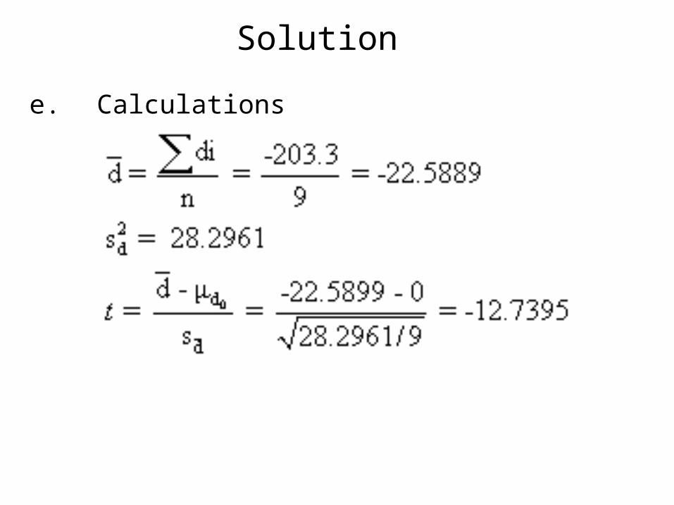
e. Calculations

Solution
f. Discussion
Reject H0 because -12.7395 < -1.8595p = 6.79 x 10⁻⁷

Solution
g. Conclusions• On the basis of these data, we conclude that the diet program is effective.• Other considerations
– a confidence interval for d can be constructed
– z can be used if the variance is known or if the
sample is large

C) Hypothesis testing of a single population proportion
When the assumptions for using a normal curve are achieved, it is possible to test hypotheses about a population proportion. When the sample size is large to permit use of the central limit theorem, the statistic of choice is z.
(continued)

Example 7.5.1
IV drug users and HIV
We wish to know if we may conclude that fewer than 5% of the IV drug users in the sampled population are HIV positive.

Solution
a. Given
n = 423 with 18 possessing the characteristic of
interest
= 18/423 = .0426p0 = .05 = .05

Solution
b. Assumptions• because of the central limit theorem, the sampling distribution of is normally distributed

Solution
c. Hypotheses
H0:p .05 HA:p < .05
(continued)

Solution
If H0 is true, p = .05 and the standard error is
Note that the standard error is not based on the value of

Solution
d. Statistical test -- Test statistic
The test statistic is z which is calculated as

Solution
Distribution
Because the sample is large we can use z distributed as the normal distribution if H0 is true.
Solution
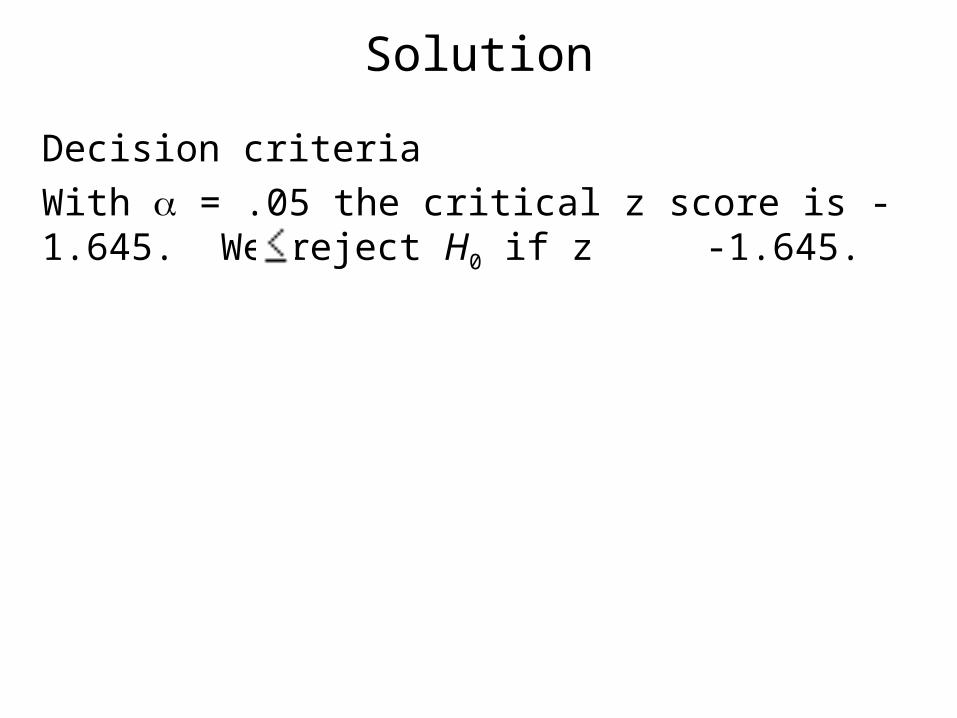
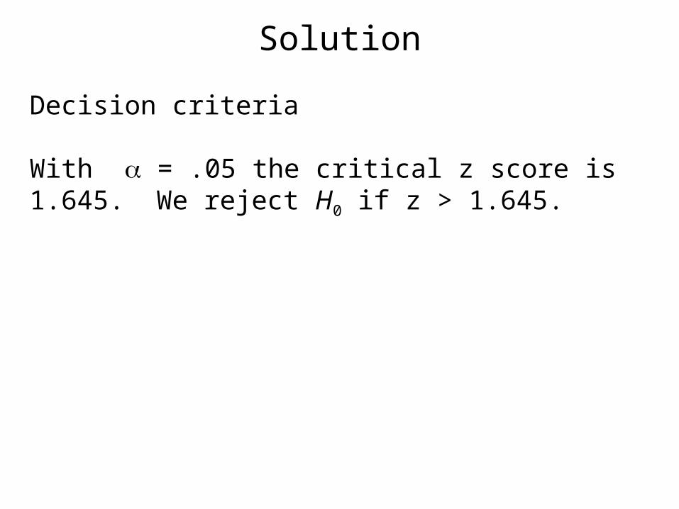
Decision criteria
With = .05 the critical z score is -1.645. We reject H0 if z -1.645.

e. Calculations

Solution
f. Discussion
Do not reject H0 because -.6983 > -1.645

Solution
(7) Conclusions
We conclude that p may be .05 or more.

D) Hypothesis testing of the difference between two population proportions
It is frequently important to test the difference between two population proportions. Generally we would test p1 = p2 . This permits the construction of a pooled estimate which is given by the following formula.
(continued)
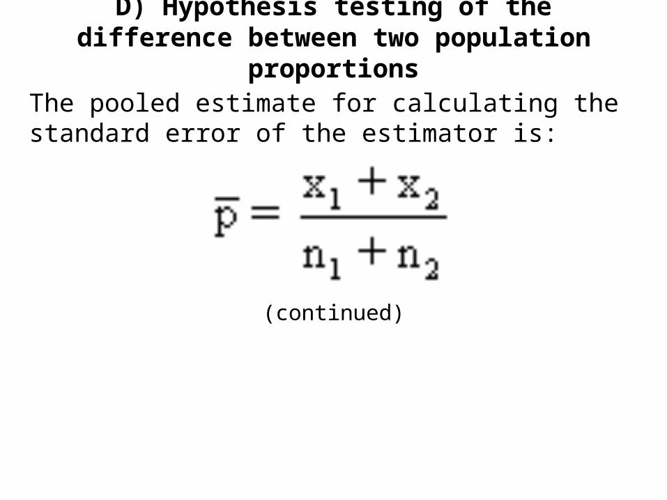
D) Hypothesis testing of the difference between two population proportions
The pooled estimate for calculating the standard error of the estimator is:
(continued)

D) Hypothesis testing of the difference between two population proportions
The standard error of the estimator is:

Two population proportions -- Example 7.6.1
In a study of patients on sodium-restricted diets, 55 patients with hypertension were studied. Among these, 24 were on sodium-restricted diets. Of 149 patients without hypertension, 36 were on sodium-restricted diets. We would like to know if we can conclude that, in the sampled population, the proportion of patients on sodium-restricted diets is higher among patients with hypertension than among patients without hypertension.

a. Given
Patients with hypertension:
n1 = 55 x1 = 24 = .4364
Patients without hypertension:
n2 = 149 x2 = 36 = .2416
= .05
Solution
b. Assumptions
independent random samples from the populations

Solution
c. Hypotheses
H0: p1 p2
HA: p1 > p2

d. Statistical test – Test statistic
The test statistic is z which is calculated as

Solution
Distribution
If the null hypothesis is true, the test statistic approximately follows the standard normal distribution.
Solution
Decision criteria
With = .05 the critical z score is 1.645. We reject H0 if z > 1.645.

e. Calculations

Solution
f. Discussion
Reject H0 because 2.71 > 1.645

Solution
g. Conclusions
The proportion of patients on sodium restricted diets among hypertensive patients is higher than in nonhypertensive patients.
p = .0034

E) Hypothesis testing of a single population variance

Where the data consist of a simple random sample drawn from a normally distributed population, the test statistic for testing hypotheses about a single population variance is
which, when H0 is true, is distributed as 2 with n-1 degrees of freedom.

Example 7.7.1
Response to allergen inhalation in allergic primates. In a study of 12 monkeys, the standard error of the mean for allergen inhalation was found to be .4 for one of the items studied. We wish to know if we may conclude that the population variance is not 4.

Solution
a. Given
n = 12 standard error = .4 = .05
df = 11

Solution
b. Assumptions• simple random sample• normally distributed population

Solution
c. Hypotheses
H0: 2 = 4
HA: 2 4

Solution
d. Statistical test -- Test statistic
The test statistic is
Solution
Distribution
When the null hypothesis is true, the distribution is
2 with 11 df.

Solution
Decision criteria
With = .05 and 11 df, the critical values are 3.816 and 21.920. Reject H0 if 2 < 3.816 or 2 > 21.920.


Solution
e. Calculations
s2 = .4*12 = 4.8
2= [11(4.8)]/4=13.2

Solution
f. Discussion
Do not reject H0 because 3.816 < 13.2 < 21.920
(calculated value of 2 is not in rejection region)

Solution
g. Conclusions
Based on these data, we cannot conclude that the population variance is not 4.
p > .05 because 2 = 13.2 is not in the rejection region.

F) Hypothesis testing of the ratio of two population variances
This test is used to determine if there is a significant difference between two variances. The test statistic is the variance ratio
(continued)

F) Hypothesis testing of the ratio of two population variances
The statistic follows the F distribution with n1 -1 numerator degrees of freedom and n2 -1 denominator degrees of freedom.

How V. R. is determined
• two tail test
The larger variance is put in the numerator.

How V. R. is determined
• one sided test H0: 12 2
2
In a one sided test where H0: 12 2
2 and
HA : 12 > 2
2 we put s12 /s2
2. The critical value of F is determined for using the appropriate degrees of freedom.

How V. R. is determined
• one sided test H0: 12 2
2
In a one sided test where H0: 12 2
2
and HA : 12 < 2
2 we put s22 /s1
2. The critical value of F is determined for using the appropriate degrees of freedom.

Example 7.8.1 – Pituitary adenomas
A study was performed on patients with pituitary adenomas. The standard deviation of the weights of 12 patients with pituitary adenomas was 21.4 kg. A control group of 5 patients without pituitary adenomas had a standard deviation of the weights of 12.4 kg. We wish to know if the weights of the patients with pituitary adenomas are more variable than the weights of the control group.

a. GivenPituitary adenomas:
n1 = 12 s1 = 21.4 kgControl:
n2 = 5 s2 = 12.4 kg
= .05

Solution
b. Assumptions• each sample is a simple random sample• samples are independent• both populations are normally distributed
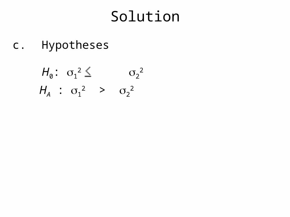
Solution
c. Hypotheses
H0: 12 2
2
HA : 12 > 2
2

Solution
Statistical test -- Test statistic
The test statistic is

Solution
Distribution
When H0 is true, the test statistic is distributed as F with 11 numerator degrees of freedom and 4 denominator degrees of freedom.
Solution
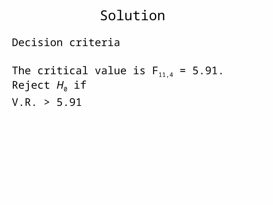
Decision criteria
The critical value is F11,4 = 5.91. Reject H0 if
V.R. > 5.91

From the F.95 table

Solution
e. Calculations

Solution
f. Discussion
We cannot reject H0 because 2.98 < 5.91. The calculated value for V.R. falls in the nonrejection region.
Solution
g. Conclusions
The weights of the population of patients may not be any more variable than the weights of the control subjects. Since V.R. of 2.98 < 3.10, it gives p > .10Actual p = .1517

fin


