Biostats II 2013 Lecture 1

8/12/2019 Biostats II 2013 Lecture 1

http://slidepdf.com/reader/full/biostats-ii-2013-lecture-1 1/19

L1.1

Biostatistics II(PUBH5769)

TOPIC 1

UNIT OVERVIEW ANDINTRODUCTORY MATERIAL

1.1 UNIT OVERVIEWThis course covers biostatistical methods commonly used in

epidemiological and clinical research.

It focuses on modern regression (and a few classical) methods for • Quantitative outcomes

• Binary outcomes

• Count (number of events) outcomes

• Time-to-event outcomes.

It considers and describes the application of these methods to data

from• cross-sectional,

• case-control,

• cohort and

• clinical studies

The emphasis is on• How to intelligently use these methods

• How to use SAS to do the calculations

• How to interpret the results

And not on

•The underlying statistical theory

•Memorising formulae



L1.2

Assumed prior knowledge and experience

• A knowledge of basic statistical methods and concepts(as taught in introductory biostatistics/statistics coursessuch as PUBH8753/4401 Biostatistics 1)

• A basic familiarity with epidemiological/clinical study designs(copy of a chapter from a book is on LMS)

• Familiarity with hand-held calculatorsYou must have your own calculator and know how to use it. Also, it must have an ‘approved’ UWA sticker to take into exam.

• Familiarity with computing in a Windows environment

• Experience with at least one statistical analysis package(such as SPSS).

SPSS

Learning outcomes

• Understand and be able to apply standard biostatisticalmethods commonly used in epidemiological and clinicalresearch including

ANOVA and multiple linear regression2 x K frequency table methods, logistic regressionIncidence rates and Poisson regression

Kaplan-Meier survival curves and Cox regression

• Be able to use the package SAS to carry out statisticalanalyses of epidemiological/clinical data.

• Understand the statistical content of articles inepidemiological/clinical literature.

PUBH5769

Biostatistics II course



L1.3

Course Reader and textbooksBiostatistics II Course Reader

• Lecture notes (pages numbered Lx.x)

• Problems, Computing and Answers (pages numbered Px.x)

• Review articles (pages numbered Rx.x)

• Introduction to SAS (pages numbered Cx.x)

• Statistical Tables (pages numbered Tx.x)

Recommended reading

> Woodward M. Epidemiology: Study design and data analysis. Chapman and Hall.

> Le CT. Introductory Biostatistics. John Wiley.

> Kahn, H.A. and Sempos, C.T. Statistical methods in epidemiology. OxfordUniversity Press.

> Dawson, B. and Trapp, R.G. Basic and clinical biostatistics. Prentice-Hall.

> Everitt, BS and Der, G. A handbook of statistical analyses using SAS.

Chapman and Hall

Lectures and TutorialsWeekly class Wednesday 9.00 -11.50am includes

• Tutorial (Starts 9am for 45 minutes)

• Lecture (Starts at 10am for 1 hour and 50 minutes with

break around 11am)

The tutorial covers the topic of the previous week’s

lecture.

Bring your calculator to the tutorial!

The Course Reader includes a copy of the lecture

presentation (so read ahead!)

ALL LECTURES SHOULD BE RECORDED AND

AVAILABLE THROUGH LMS FOR PLAYBACK

ANYTIME.



L1.4

Computing and SASThe statistics package is SAS.

The Course Reader contains a self-explanatory Introduction to SAS. Sign up for anIntroduction to SAS Session with Mark Divitini if you want help with gettingstarted.

The expectation is that you do the SAS computing activities on your own (orpreferably with a class mate) at a place and time that suits you. Some of theProblems in the Course reader involve using SAS.

SAS is available on the computers in theSPH Postgrad Computer Lab (Rm 1.27, Clifton St Building) for SPH students onlySPH Main Computer Lab on the Nedlands Campus next to cafeteria (all students)

Bring a USB flash drive to save and keep your work!

If you use SAS elsewhere, download a copy of the files (datasets and programs) from

LMS or email Mark Divitini and he will send them to you.UWA has a site license for SAS and all enrolled students can get a copy. See LMS

for more details and forms.

If you need help with SAS during the semester, email Mark Divitini with yourquestions or to arrange a time to see him.

SAS

Assessment

• Three assignments each 20% (Due Sept 4, Oct 9, Nov 1)

• Final (written) examination 40% (Exam period Nov 9-23)

• Assignments involve data analysis using hand-calculation as well asSAS, providing written answers to questions that test understanding,and reviewing articles from the literature.

Hand assignments (with cover sheet) to SPH Reception.There is a penalty for (unapproved) late assignments.

• The final exam involves providing written answers to problems. Many

will involve use of a hand-calculator. Some will include SAS output.The exam is “open book”.



L1.5

LMSwww.lms.uwa.edu.au

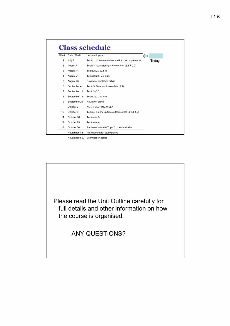
• All supplementary unit materials are placed on LMS(including assignments)

• The recording of the lecture should be available soon after thelecture has finished (same day).

• All students enrolled for credit (i.e. doing assessment) areautomatically given permission to access the LMS unit materials.Others who need access should contact lecturer (and provide anemail address).

Study plan and workload• Study each topic each week by reviewing the lecture notes, reading

appropriate sections of the books, doing the related SAS computing,and doing the problems in the course reader.

• Attempt the problems before coming to the tutorial.

• Begin assignments early, don’t leave until last few days.

• You should spend about 9 hours per week on this course

Tutorial (1 hour)

Lecture (2 hours)

Computing (1-2 hours)

Private study and assignments (4-5 hours)



L1.6

Today

Class scheduleWeek Date (Wed) Lectur e topi cs

1 July 31 Topic 1: Course overview and introductory material

2 August 7 Topic 2: Quantitative outcome data (2.1 & 2.2)

3 August 14 Topic 2 (2.3 & 2.4)

4 August 21 Topic 2 (2.5, 2.6 & 2.7)

5 August 28 Review of published article

6 September 4 Topic 3: Binary outcome data (3.1)

7 September 11 Topic 3 (3.2)

8 September 18 Topic 3 (3.3 & 3.4)

9 September 25 Review of article

October 2 NON-TEACHING WEEK

10 October 9 Topic 4: Follow-up time outcome data (4.1 & 4.2)

11 October 16 Topic 4 (4.3)

12 October 23 Topic 4 (4.4)

13 October 30 Review of article & Topic 5: course wind-up

November 4-8 Pre-examination study period

November 9-23 Examination period

Please read the Unit Outline carefully for

full details and other information on how

the course is organised.

ANY QUESTIONS?



L1.7

1.2 INTRODUCTORY MATERIALTYPE OF OUTCOME VARIABLEThe type of outcome variable determines the method of

statistical analysis.

There are four main types:

• Quantitative eg. blood pressure

• Binary eg. disease / disease free

• Number of events eg. number of deaths

for a group• Time to event eg. time to death (possibly censored)

• The focus in this unit is on analysing data on these

outcome variables using modern regression modelling

methods.

• However, a few classical methods (for proportions and

group incidence rates) that are still in common use arealso included.

• The regression model for an outcome variable is based

on a particular summary measure and a measure of effect



L1.8

Quantitative outcome variable

Example: measured systolic blood pressure (SBP)

Summary measure: mean

Effect measure: difference in means

Regression method: linear regression

Examples of linear regression models

Mean (SBP) = + 1 Age

1 = Difference in mean (SBP) if Age increases by 1 year

Mean (SBP) = + 1[if group=control] + 2 [if group=treated]

1 - 2 = Difference in mean (SBP) for control vs treated groups

Binary outcome variable

Example: disease / disease free

Summary measure: proportion

Effect measure: odds ratio

Regression method: Logistic regression

Prevalence and risk are proportions (p).

personsof number totalcasesexistingof number Prevalence

eg. Prevalence of diabetes in WA women aged 60-69 years in 1990 is 0.047 or 4.7%.

beginningatriskatpersonsof number total

timeof periodincasesnewof number Risk

eg. Risk of 50 years old woman having a stroke in next 10 years is 0.02 or 2%.

Odds = p/(1-p) and Odds ratio)p-(1p

)p-(1pOR

22

11



L1.9

Binary outcome variable (ctd)

Example: disease / disease free

Summary measure: proportion

Effect measure: odds ratio

Regression method: Logistic regression

Examples of logistic regression models

log (odds of disease) = + 1 Age

1 = Difference in log (odds of disease) if Age increases by 1 year

= ratio of odds of disease if Age increases by 1 year

= 1.05 ie odds of disease increases by 5% each year of age

log (odds of disease) = + 1[if group=control] + 2 [if group=treated]

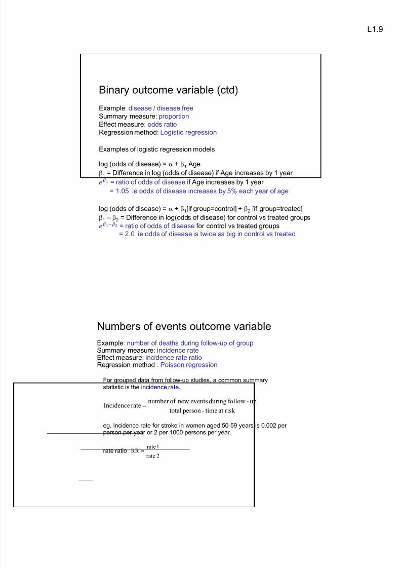
1 – 2 = Difference in log(odds of disease) for control vs treated groups

= ratio of odds of disease for control vs treated groups

= 2.0 ie odds of disease is twice as big in control vs treated

Numbers of events outcome variable

Example: number of deaths during follow-up of groupSummary measure: incidence rateEffect measure: incidence rate ratioRegression method : Poisson regression

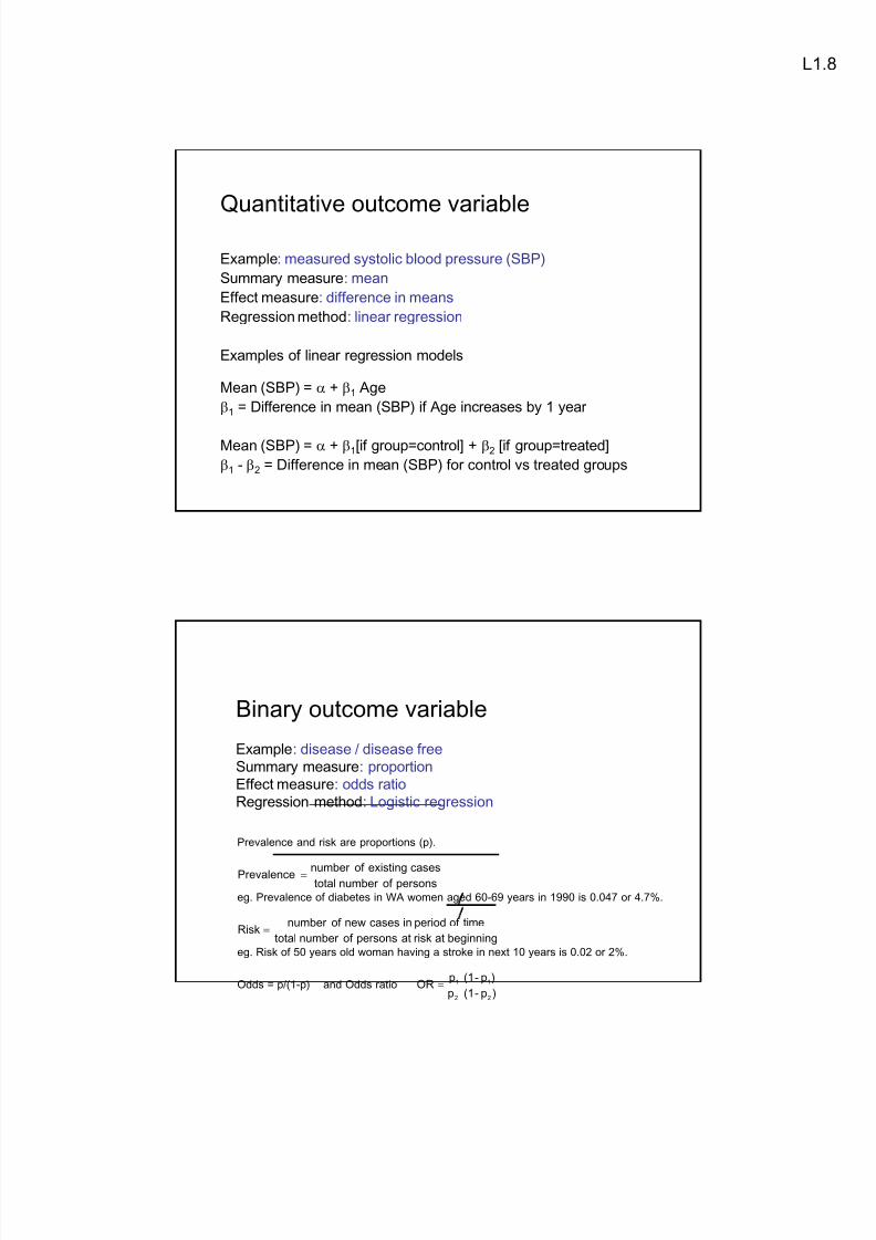
For grouped data from follow-up studies, a common summarystatistic is the incidence rate.

risk attime- persontotal

up-followduringeventsnewof numberrateIncidence

eg. Incidence rate for stroke in women aged 50-59 years is 0.002 perperson per year or 2 per 1000 persons per year.

rate ratio2rate

1rateRR



L1.10

Numbers of events outcome variable (ctd)

Example: number of deaths during follow-up of groupSummary measure: incidence rateEffect measure: incidence rate ratioRegression method : Poisson regression

Examples of Poisson regression models

log (rate) = + 1 Age

1 = Difference in log (rate) if Age increases by 1 year

= ratio of rates if Age increases by 1 year

= 1.05 ie rate increases by 5% each year of age

log (rate) = + 1[if group=control] + 2 [if group=treated]

1 – 2 = Difference in log(rate) for control vs treated groups

= ratio of rates for control vs treated groups

= 2.0 ie rate is twice as big in control vs treated

Time to event outcome variable

Example: time to death (possibly censored)

Summary measure: survival curve

Effect measure: hazard rate ratio

Regression method : Cox regression

A common summary of the time-to-event data for a group is the survivalcurve.

S(t) = the proportion who have not had event by time t.

However, the comparison and modelling of survival curves is usually basedon the analysis of the magnitude of hazard ratios.

h(t) = hazard at time t is the risk of having event over the next instant givenevent-free up to time t.

Hazard ratio(t)h

(t)hHR

2

1 is the 'effect' size

and it is commonly assumed this does not change with time t (calledproportional hazards assumption).



L1.11

Time to event outcome variable (ctd)

Example: time to death (possibly censored)

Summary measure: survival curve

Effect measure: hazard rate ratio

Regression method : Cox regression

Examples of Cox regression models

log (hazard at t) = (t) + 1 Age

1 = Difference in log (hazard) if Age increases by 1 year

= ratio of hazards if Age increases by 1 year

= 1.05 ie hazard increases by 5% each year of age

log (hazard at t) = (t) + 1[if group=control] + 2 [if group=treated]

1 – 2 = Difference in log(hazard) for control vs treated groups

= ratio of hazards for control vs treated groups

= 2.0 ie hazard is twice as big in control vs treated

Study designsObservational studies

• cross-sectional (point in time)

• case-control (retrospective)

• cohort (prospective)

Intervention studies (experiments)

• health promotion / disease prevention trial

• therapeutic clinical trial

Cross-sectional study prevalence, mean

Case-control study odds ratio

• prevalent cases odds of being diseased

• incident cases odds of developing disease

Cohort and intervention studies risk, rate, mean



L1.12

Statistical inference

)(statistic

sample statistical inference

)(parameter

population

value)-pstatistic,test,hypothesis(nulltestinghypothesis

CI) SE, estimate,( estimation

inference

lstatistica

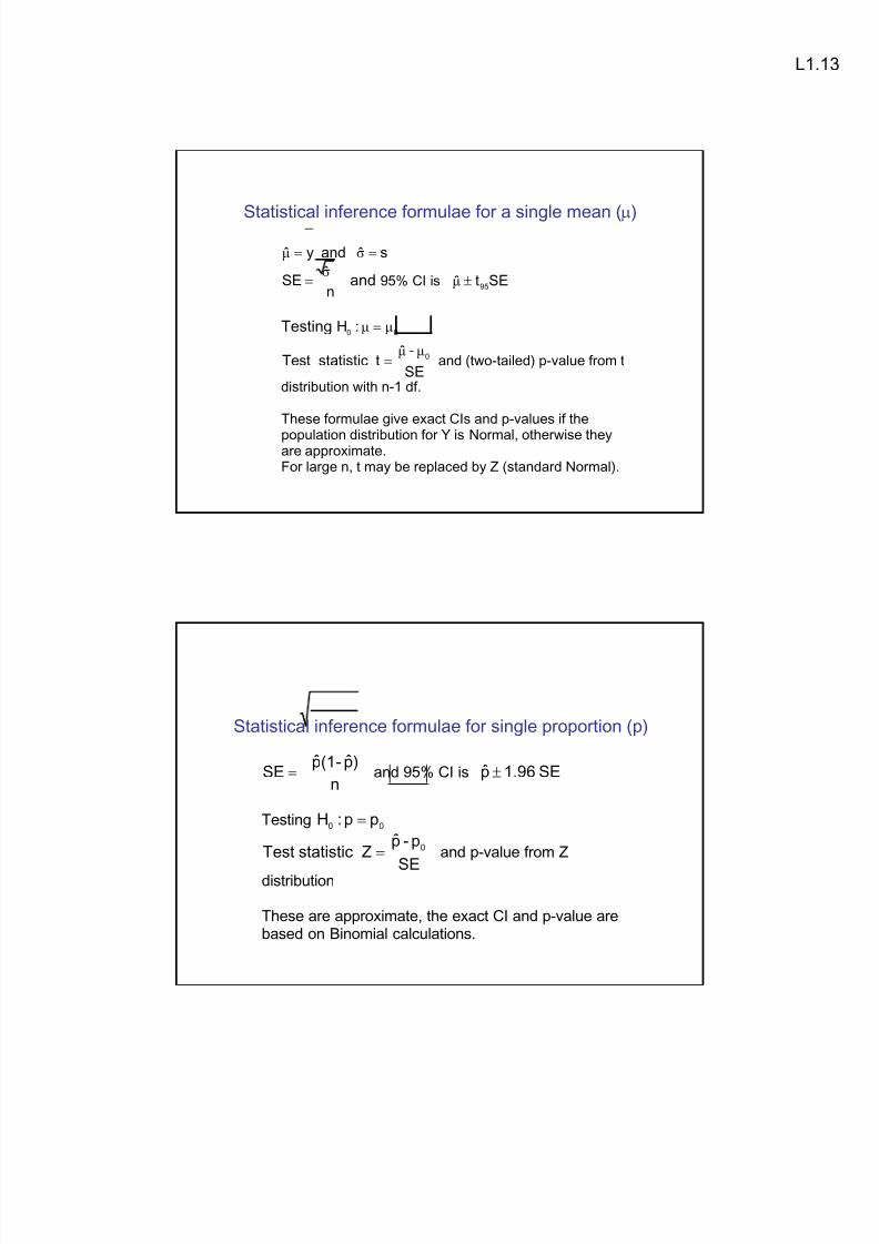
CIs and p-values are calculated from the sampling distributions of theestimator and test statistic.The 95% CI indicates how well we have estimated a populationparameter. Narrower CIs indicate greater accuracy.P-values measure the amount of evidence in the sample data against

the null hypothesis. The closer the p-value to zero, the greater theevidence.

Most of the commonly used CI and p-value formulae are based on theassumption that the estimator (or a transformation of it) has a Normalsampling distribution. For moderate and large sample sizes, this isapproximately true.

General formulaeThe general form of these approximate formulae for a single parameter is

95% CI estimate (Z95 or t95) x SE with Z95=1.96

SE

valueedhypothesis-estimate statisticTest

With p-value from Z (or t) distribution

Most (but not all) approximate formulae come from asymptotic likelihood theory

which provides an estimator (maximum likelihood estimator MLE)

an approximate standard error (and hence a 95% CI)

and three approximate p-value formulae (Wald, Score, Likelihood ratio)

The p-value method described above is the Wald p-value.

When we are testing hypotheses involving more than one p arameter , the teststatistic often has an asymptotic chi-squared distribution.When we are comparing variances, the test statistic often has an F distribution.



L1.13

Statistical inference formulae for a single mean ()

sˆ and yˆ σμ

n

ˆ SE σ and 95% CI is SEtˆ 95

μ

Testing 00 :H μμ

SE

-ˆtstatisticTest 0μμ and (two-tailed) p-value from t

distribution with n-1 df.

These formulae give exact CIs and p-values if the

population distribution for Y is Normal, otherwise theyare approximate.For large n, t may be replaced by Z (standard Normal).

Statistical inference formulae for single proportion (p)

n

)p̂-(1p̂ SE and 95% CI is SE1.96p̂

Testing00

pp:H

SE

p-p̂ZstatisticTest 0 and p-value from Z

distribution

These are approximate, the exact CI and p-value arebased on Binomial calculations.



L1.14

Statistical inference formulae for single rate ()

T

ˆ SE λ

and 95% CI is SE1.96ˆ λ

where T = total person-time

Testing 00 :H λ λ

SE

-ˆZstatisticTest

0λ λ

and p-value from Z

distribution

These are approximate, the exact CI and p-value are

based on Poisson calculations.

Statistical inference formulae in other situations

Formulae for estimation and testing of “effect” measures insimple situations such as the comparison of two groups arereadily available (and can also be done on hand-calculator).

Comparing two means via difference (see Section 2.1)Comparing two proportions via odds ratio (see section 3.1)

Comparing two rates via rate ratio (see section 4.1)Comparing two survival curves (see section 4.3)

In more complex situations the formulae are more complicatedand we must rely on computer programs to obtain the estimate,its SE, its 95% CI and the test statistic value.



L1.15

Probability distributions and

statistical tables

The hand-calculation methods throughout the unit sometimes involve

looking up statistical tables for specific probability distributions, usually

to obtain the p-value associated with a particular value of the test

statistic, but sometimes to get the SE multiplier for a 95% confidence

interval.

The probability distributions used in this unit are

Standard Normal distribution (Z)

t- distribution (t)

Chi-squared distribution (2)F- distribution (F)

Tables for these distributions and how to use these tables are provided

in Course Reader .

Datasets used throughout semester

Data set Files

Diabetes data diabet.dat and diabet.sas

Busselton 1981 survey data bsn81.dat and bsn81.sas

US city air pollution data so2cit.dat

BCG case-control data bcg.sas

Endometrial cancer case-control data endomet.dat and endomet.sas

Grouped smoking death cohort data smokdth.sas

Lymphoma survival data lymphoma.sas

filename.sas is a SAS program file (which sometimes includes data)

filename.dat is a data file



L1.16

Diabetes data

The diabetes dataset relates to baseline and mortality follow-up datafor a cohort of 498 persons with diabetes.

AGE age in years

SEX 0 = female1 = male

DURATION duration of diabetes in years

TREAT 1 = insulin injections2 = tablets3 = special diet

PDW percent of desirable weight

SBP systolic blood pressure in mmHg

HAEM glycosylated haemoglobin inmmol/L

DIED5 0 = have not died within 5 years1 = died within 5 years

First 4 rows of diabet.dat

41 1 12 2 99.7 132 10.6 0

47 0 3 2 134.3 170 12.2 0

62 1 5 2 143.6 170 10.6 0

69 0 3 1 135.6 170 10.8 0

Numbers separated by spaces

SAS program to produce summary of data

data di abet es;i nf i l e ‘ C: \ Bi ost at 2\ di abet . dat ' ;i nput age sex dur at i on t r eat pdw sbp haem di ed5;

run; proc means dat a=di abet es maxdec=3;run;

The MEANS Procedure

Variable N Mean Std Dev Minimum Maximum

ƒƒƒƒƒƒƒƒƒƒƒƒƒƒƒƒƒƒƒƒƒƒƒƒƒƒƒƒƒƒƒƒƒƒƒƒƒƒƒƒƒƒƒƒƒƒƒƒƒƒƒƒƒƒƒƒƒƒƒ

age 498 63.873 9.550 40.000 80.000

sex 498 0.554 0.498 0.000 1.000

duration 498 8.092 6.426 1.000 39.000

treat 498 1.859 0.672 1.000 3.000

pdw 498 123.594 14.336 76.600 149.900

sbp 498 152.442 21.560 98.000 198.000

haem 498 10.652 2.022 6.300 18.800

died5 498 0.215 0.411 0.000 1.000

ƒƒƒƒƒƒƒƒƒƒƒƒƒƒƒƒƒƒƒƒƒƒƒƒƒƒƒƒƒƒƒƒƒƒƒƒƒƒƒƒƒƒƒƒƒƒƒƒƒƒƒƒƒƒƒƒƒƒƒ

Must be in data

file order

Location of file

Note: mean of died5 = proportion of values equal to 1



L1.17

Busselton 1981 survey data

AGE age in years (range 40-69)

ALCGRAMS alcohol consumed per week in grams

ANGINA ever had angina 0 = no, 1 = yes

ASTHMA ever had asthma 0 = no, 1 = yes

BMI body mass index (weight/height2) in kg/m

2

BRONCH ever had bronchitis 0 = no, 1 = yes

CHOL blood cholesterol in mmol/L

CIGSDAY number of cigarettes smoked per day

CVDCENS died from cardiovascular disease 0 = no, 1 = yes

DBP diastolic blood pressure in mmHg

DIABETES have diabetes 0 = no, 1 = yes

DRINKING 1 = never, 2 = ex, 3= < 20 grams/day4 = 20 – 60 grams/day, 5 = > 60 grams/day

DTHCENS died during follow-up 0 = no, 1 = yes

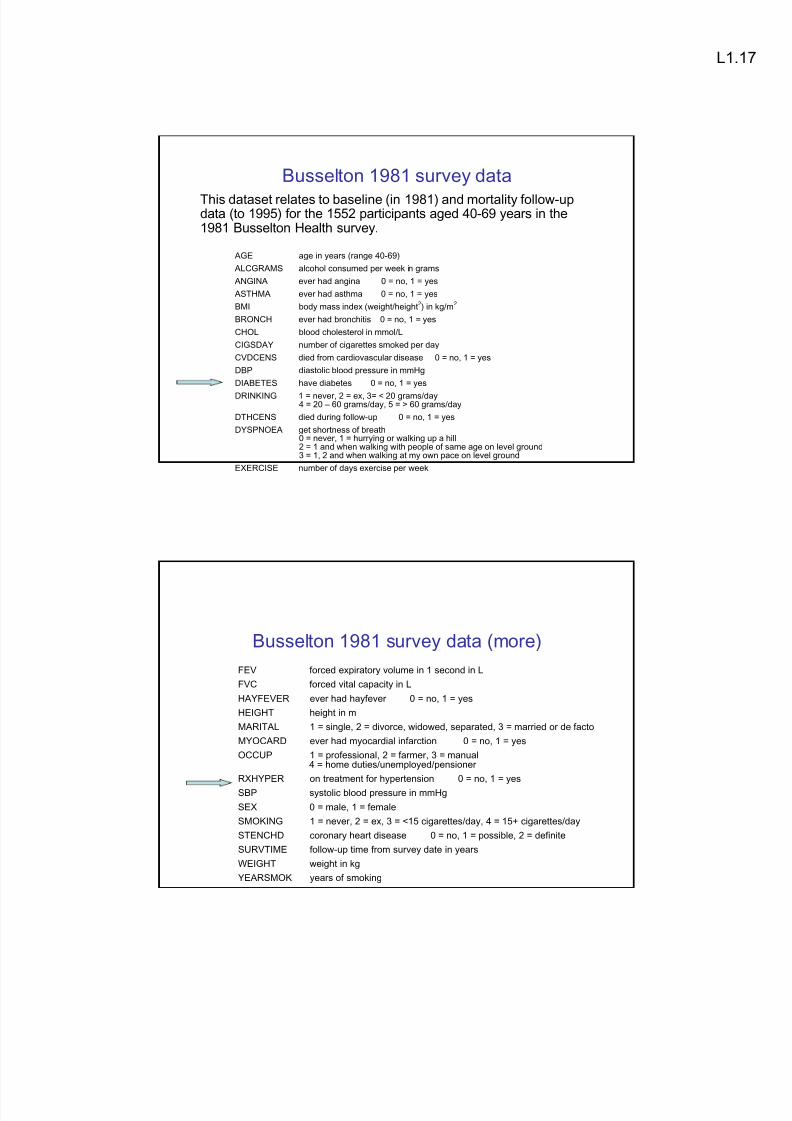
DYSPNOEA get shortness of breath0 = never, 1 = hurrying or walking up a hill2 = 1 and when walking with people of same age on level ground3 = 1, 2 and when walking at my own pace on level ground

EXERCISE number of days exercise per week

This dataset relates to baseline (in 1981) and mortality follow-updata (to 1995) for the 1552 participants aged 40-69 years in the1981 Busselton Health survey.

Busselton 1981 survey data (more)

FEV forced expiratory volume in 1 second in L

FVC forced vital capacity in L

HAYFEVER ever had hayfever 0 = no, 1 = yes

HEIGHT height in m

MARITAL 1 = single, 2 = divorce, widowed, separated, 3 = married or de facto

MYOCARD ever had myocardial infarction 0 = no, 1 = yes

OCCUP 1 = professional, 2 = farmer, 3 = manual4 = home duties/unemployed/pensioner

RXHYPER on treatment for hypertension 0 = no, 1 = yes

SBP systolic blood pressure in mmHg

SEX 0 = male, 1 = female

SMOKING 1 = never, 2 = ex, 3 = <15 cigarettes/day, 4 = 15+ cigarettes/day

STENCHD coronary heart disease 0 = no, 1 = possible, 2 = definite

SURVTIME follow-up time from survey date in years

WEIGHT weight in kg

YEARSMOK years of smoking



L1.18

SAS summary of bsn81 data

The MEANS Procedure

Variable N Mean Std Dev Minimum Maximumƒƒƒƒƒƒƒƒƒƒƒƒƒƒƒƒƒƒƒƒƒƒƒƒƒƒƒƒƒƒƒƒƒƒƒƒƒƒƒƒƒƒƒƒƒƒƒƒƒƒƒƒƒƒƒƒƒƒƒƒ

age 1552 55.816 8.486 40.020 69.980

alcgrams 1552 89.470 156.437 0.000 2450.000

angina 1552 0.037 0.188 0.000 1.000asthma 1552 0.075 0.263 0.000 1.000

bmi 1552 26.100 3.963 16.800 45.300

bronch 1552 0.193 0.395 0.000 1.000

chol 1552 6.151 1.169 3.010 14.410cigsday 1552 3.233 7.968 0.000 70.000

cvdcens 1552 0.050 0.219 0.000 1.000

dbp 1552 79.259 11.857 30.000 178.000

diabetes 1552 0.025 0.157 0.000 1.000drinking 1552 2.624 1.081 1.000 5.000

dthcens 1552 0.114 0.318 0.000 1.000

dyspnoea 1552 0.387 0.752 0.000 3.000

exercise 1552 3.110 2.932 0.000 7.000fev 1552 2.623 0.818 0.300 5.900

fvc 1552 3.490 0.961 1.000 7.200

hayfever 1552 0.189 0.392 0.000 1.000height 1552 1.665 0.086 1.440 1.920

marital 1552 2.860 0.415 1.000 3.000myocard 1552 0.017 0.128 0.000 1.000

occup 1552 3.229 1.134 1.000 4.000rxhyper 1552 0.188 0.390 0.000 1.000

sbp 1552 131.182 19.392 84.000 223.000

sex 1552 0.557 0.497 0.000 1.000

smoking 1552 1.800 1.004 1.000 4.000stenchd 1552 0.348 0.639 0.000 2.000

survtime 1552 13.368 2.459 0.340 14.120

weight 1552 72.558 13.258 37.800 126.000

yearsmok 1552 14.135 16.764 0.000 56.000

ƒƒƒƒƒƒƒƒƒƒƒƒƒƒƒƒƒƒƒƒƒƒƒƒƒƒƒƒƒƒƒƒƒƒƒƒƒƒƒƒƒƒƒƒƒƒƒƒƒƒƒƒƒƒƒƒƒƒƒƒ

Busselton Health Study websitehttp://www.busseltonhealthstudy.com/



L1.19

BEFORE NEXT WEEK• Get a Course Reader(if still don’t have one)

• Get or borrow a hand-calculator

• Attempt Topic 1 problems

• Do Intro to SAS session

• Get a USB flash drive?

• Get a text book?

• Review how to use statistical tables for Normal and t-

distributions.

• Arrange SAS for your own PC and get course files.

Date post:	03-Jun-2018
Category:	Documents
Upload:	ben-harvey
View:	234 times
Download:	0 times

Biostats II 2013 Lecture 1

Documents