BIRKHOFF NORMAL FORM FOR PDEs WITH TAME MODULUS D. Bambusi, B. Gr´ ebert 13.10.04 Abstract We prove an abstract Birkhoff normal form theorem for Hamiltonian Partial Differential Equations. The theorem applies to semilinear equa- tions with nonlinearity satisfying a property that we call of Tame Modulus. Such a property is related to the classical tame inequality by Moser. In the nonresonant case we deduce that any small amplitude solution remains very close to a torus for very long times. We also develop a general scheme to apply the abstract theory to PDEs in one space dimensions and we use it to study some concrete equations (NLW,NLS) with different boundary conditions. An application to a nonlinear Schr¨ odinger equation on the d-dimensional torus is also given. In all cases we deduce bounds on the growth of high Sobolev norms. In particular we get lower bounds on the existence time of solutions. Contents 1 Introduction 3 2 Statement of the abstract result 6 2.1 Tame maps .............................. 6 2.2 The modulus of a map ........................ 8 2.3 The theorem ............................. 9 3 Applications 12 3.1 An abstract model of Hamiltonian PDE .............. 12 3.2 Nonlinear wave equation ....................... 15 3.2.1 Dirichlet boundary conditions ................ 16 3.2.2 Periodic boundary conditions ................ 16 3.3 NLS in 1 dimension ......................... 19 3.4 Coupled NLS in 1 dimension .................... 20 3.5 NLS in arbitrary dimension ..................... 21 1
Transcript
BIRKHOFF NORMAL FORM FOR PDEs
WITH TAME MODULUS
D. Bambusi, B. Grebert
13.10.04
Abstract
We prove an abstract Birkhoff normal form theorem for HamiltonianPartial Differential Equations. The theorem applies to semilinear equa-tions with nonlinearity satisfying a property that we call of Tame Modulus.Such a property is related to the classical tame inequality by Moser. In thenonresonant case we deduce that any small amplitude solution remainsvery close to a torus for very long times. We also develop a general schemeto apply the abstract theory to PDEs in one space dimensions and we useit to study some concrete equations (NLW,NLS) with different boundaryconditions. An application to a nonlinear Schrodinger equation on thed-dimensional torus is also given. In all cases we deduce bounds on thegrowth of high Sobolev norms. In particular we get lower bounds on theexistence time of solutions.
4 Proof of the Normal Form Theorem 234.1 Properties of the functions with tame modulus . . . . . . . . . . 244.2 The main lemma and conclusion of the proof . . . . . . . . . . . 29
B On the verification of the tame modulus property 51
2
1 Introduction
During the last fifteen years remarkable results have been obtained in perturba-tion theory of integrable partial differential equation. In particular the existenceof quasiperiodic solutions has been proved through suitable extensions of KAMtheory (see [Kuk87, Kuk93, Kuk00, Way90, Cra00, KP03, CW93, Bou03]). How-ever very little is known on the behavior of the solutions lying outside KAMtori. In the finite dimensional case a description of such solutions is providedby Nekhoroshev’s theorem whose extension to PDEs is at present a completelyopen problem. In the particular case of a neighbourhood of an elliptic equilib-rium point, Birkhoff normal form theorem provides a quite precise descriptionof the dynamics. In the present paper we give an extension of Birkhoff normalform theorem to the infinite dimensional case and we apply it to some semilinearPDEs in one or more space dimensions.
To start with consider a finite dimensional Hamiltonian system H = H0 +Pwith quadratic part
H0 =n∑j=1
ωjp2j + q2j
2, ωj ∈ R
and P a smooth function having a zero of order at least three at the origin. Theclassical Birkhoff normal form theorem states that, for each r ≥ 1, there exits areal analytic symplectic transformation Tr such that
H Tr = H0 + Z +Rr, (1.1)
where the remainder Rr has a zero of order r + 3 and Z is a polynomial ofdegree r + 2. Provided the frequencies are nonresonant, Z depends on theactions Ij = (p2
j + q2j )/2 only, and one says that the Hamiltonian (1.1) is inintegrable Birkhoff normal form up to order r+2. As a dynamical consequence,solutions with initial data of size ε 1 remain at distance 2ε from the originfor times of order ε−r, and the actions remain almost constant during the samelapse of time. Moreover any solution remains εr1 close to a torus of maximaldimension up to times of order ε−r2 , with r1 + r2 = r + 1.
The proof of such a standard theorem is obtained by applying a sequence ofcanonical transformations that eliminate order by order the non normalized partof the nonlinearity. Remark that, since the space of homogeneous polynomialsof any finite order is finite dimensional, only a finite number of monomials haveto be removed. Of course this is no more true in the infinite dimensional case.
To generalize Birkhoff normal form theory to infinite dimensional systems,the main difficulty consists in finding a nonresonance property that is satisfied inquite general situations and that allows to remove from the nonlinearity all therelevant non-normalized monomials. This problem has been solved by the firstauthor in a particular case, namely the nonlinear wave equation (see [Bam03b]),by remarking that most of the monomials are “not relevant”, since their vectorfield is already small. Moreover all the remaining monomials can be eliminatedusing a suitable nonresonance condition.
3
In the present paper we generalize the procedure of [Bam03b] to obtain anabstract result that can be applied to a wide class of PDEs. The idea is againthat a large part of the nonlinearity is ‘not relevant’, but we show here that thisis due to the so called tame inequality, namely
‖uv‖Hs ≤ Cs (‖u‖Hs ‖v‖H1 + ‖v‖Hs ‖u‖H1) , (1.2)
on which we base our construction. The point is that, if u =∑
|j|≥N ujeijx,
then, by (1.2) one has ∥∥u2∥∥Hs ≤
‖u‖2Hs
Ns−1
which is small provided N and/or s are large. This remark allows to forget alarge part of the nonlinearity. However in order to exploit (1.2) one has to showthat the tame property is not lost along the iterative normalization procedure.We prove that this is the case for a class of nonlinearities that we call of tamemodulus (see definition 2.6).
In our abstract theorem we show that, if the nonlinearity has tame modulus,then it is always possible to put H in the form (1.1), where the remainder termRr is of “order” r + 5/2 and Z is a polynomial of degree r + 2 containing onlymonomials which are “almost resonant” (see definition 2.12). If the frequenciesfulfill a nonresonance condition similar to the second Melnikov condition, thenH can be put in integrable Birkhoff normal form, i.e. Z depends on the actionsonly. We will also show how to deduce some informations on the dynamics whensome resonances or almost resonances are present (see sections 3.2.2, 3.5 below).
When applying this abstract Birkhoff normal form result to PDEs, one meetstwo difficulties: (1) to verify the tame modulus condition; (2) to study thestructure of Z in order to extract dynamical informations (e.g. by showing thatit depends on the actions only).
Concerning (1), in the context of PDEs with Dirichlet or periodic boundaryconditions, we obtain a simple condition ensuring tame modulus. Thus weobtain that typically all local functions and also convolution type nonlinearitieshave the tame modulus property.
The structure of Z depends on the resonance relations among the frequen-cies. Their study is quite difficult since, at variance with respect to the case ofKAM theory for PDEs, infinitely many frequencies are actually involved. Herewe prove that in the case of NLW and NLS in one space dimensions with Dirich-let boundary conditions Z is typically integrable. Thus all the small initial datagive rise to solutions that remain small and close to a torus for times of orderε−r, where ε measures the size of the initial datum and r is an arbitrary integer(see corollary 2.16 for precise statements).
In the case of periodic boundary conditions the nonresonance condition istypically violated. This is due to the fact that the periodic eigenvalues of aSturm Liouville operator are asymptotically double. Nevertheless we provethat, roughly speaking, the energy transfers are allowed only between pairs ofmodes corresponding to almost double eigenvalues (see theorem 3.16 for a pre-cise statement in the case of periodic NLW equation). In particular we deduce
4
an estimate of higher Sobolev norms as in the Dirichlet case. We also study asystem of coupled NLS’s with indefinite energy, getting the same result as in thecase of the wave equation with periodic boundary conditions. In particular wethus obtain long time existence of solutions somehow in the spirit of the almostglobal existence of [Kla83].
Finally we apply our result to NLS in higher dimension. However, in order tobe able to control the frequencies, we have to assume that the linear part is verysimple from a spectral point of view. Namely the linear operator we considerreads −∆u+V ∗u, involving a convolution operator instead of the more naturalproduct operator. In this context we again obtain long time existence andbounds on the energy exchanges among the modes (see theorem 3.25).
Previous results related to the present one were obtained by Bourgain [Bou00]who showed that, in perturbations of the integrable NLS, one has that mostsmall amplitude solutions remain close to tori for long times. Such a result isproved by exploiting the idea that most monomials in the nonlinearity are al-ready small (as in the present paper and in [Bam03b]). However the techniqueof [Bou00] seems to be quite strongly related to the particular problem dealtwith in that paper.
Other Birkhoff normal form results were presented in [Bam03a, Bam03c].Those results apply to much more general equations (quasilinear equations inhigher space dimensions) but the kind of normal form obtained in those papersonly allows to describe the dynamics up times of order ε−1. This is due tothe fact that in the normal form of [Bam03a, Bam03c] the remainder Rr has avector field which is unbounded and greatly reduces regularity. On the contraryin the present paper the result obtained allows to control the dynamics for muchlonger times.
We point out that the study of the structure of the resonances is based onan accurate study of the eigenvalues of Sturm–Liouville operators. A typicaldifficulty met here is related to the fact that the eigenvalues of Sturm–Liouvilleoperators have very rigid asymptotic properties. In order to prove our non-resonance type conditions we use ideas from degenerate KAM theory (as in[Bam03a]) and ideas from the paper [Bou96].
Acknowledgements DB was supported by the MIUR project ‘Sistemi dinamicidi dimensione infinita con applicazioni ai fondamenti dinamici della meccanicastatistica e alla dinamica dell’interazione radiazione materia’. We would like tothank Thomas Kappeler and Livio Pizzocchero for some useful discussions.
5
2 Statement of the abstract result
We will study a Hamiltonian system of the form
H(p, q) := H0(p, q) + P (p, q) , (2.1)
H0 :=∑l≥1
ωl(p2l + q2l )
2, (2.2)
where the real numbers ωl play the role of frequencies and P has a zero of orderat least three at the origin. The formal Hamiltonian vector field of the system isXH := (− ∂H
∂qk, ∂H∂pk
). Define the Hilbert space `2s(R) of the sequences x ≡ xll≥1
with xl ∈ R such that‖x‖2s :=
∑l≥1
l2s|xl|2 <∞ (2.3)
and the scale of phase spaces Ps(R) := `2s(R)⊕ `2s(R) 3 (p, q). We assume thatP is of class C∞ from Ps(R) into R for any s large enough. We will denote byz ≡ (zl)l∈Z, Z := Z− 0 the set of all the variables, where
z−l := pl , zl := ql l ≥ 1 .
and by BR,s(R) the open ball centered at the origin and of radius R in Ps(R).Often we will simply write
Ps ≡ Ps(R) , Bs(R) ≡ BR,s(R) .
Remark 2.1. In section 3, depending on the concrete example we will consider,the index l will run in N, Z or even Zd. In this abstract section we will considerindexes in N. Clearly one can always reduce to this case relabelling the indexes.
2.1 Tame maps
Let f : Ps → R be a homogeneous polynomial of degree r; we recall that f iscontinuous and also analytic if and only if it is bounded, namely if there existsC such that
|f(z)| ≤ C ‖z‖rs , ∀z ∈ Ps .
To the polynomial f it is naturally associated a symmetric r-linear form f suchthat
(and analytic) if and only if f is bounded.Given a polynomial vector field X : Ps → Ps homogeneous of degree r we
write it asX(z) =
∑l∈Z
Xl(z)el
where el ∈ Ps is the vector with all components equal to zero but the l−th onewhich is equal to 1. Thus Xl(z) is a real valued homogeneous polynomial ofdegree r. Consider the r-linear symmetric form Xl and define X :=
∑l Xlel, so
thatX(z, ..., z) = X(z) . (2.8)
Again X : Ps → Ps is analytic if and only if it is bounded. Then the same istrue for X.
Definition 2.2. Let X : Ps → Ps be a homogeneous polynomial of degree r;let s ≥ 1, then we say that X is an s–tame map if there exists a constant Cssuch that∥∥∥X(z(1), ..., z(r))
∥∥∥s
≤ Cs
r∑l=1
∥∥∥z(1)∥∥∥
1....∥∥∥z(l−1)
∥∥∥1
∥∥∥z(l)∥∥∥s
∥∥∥z(l+1)∥∥∥
1...∥∥∥z(r)
∥∥∥1
∀z(1), ..., z(r) ∈ Ps (2.9)
If a map is s–tame for any s ≥ 1 then it will be said to be tame.
Example 2.3. Given a sequence z ≡ (zl)l∈Z consider the map
(zl) 7→ (wk) , wk :=∑l
zk−lzl (2.10)
this is a tame s map for any s ≥ 1. To see this define the map1
Ps 3 zl 7→ u(x) :=∑l
zleilx ∈ Hs(T) (2.11)
where the Sobolev space Hs(T) is the space of periodic functions of period 2πhaving s weak derivatives of class L2. Then the map (2.10) is transformed intothe map
u 7→ u2
1In fact, for z ∈ Ps the index l runs in Z − 0, but one can reorder the indexes so thatthey run in Z.
7
The corresponding bilinear form is (u, v) 7→ uv and, by Moser inequality, onehas
‖uv‖Hs ≤ Cs (‖u‖Hs ‖v‖H1 + ‖v‖Hs ‖u‖H1) (2.12)
Example 2.4. According to definition 2.2, any bounded linear map A : Ps → Psis s-tame.
2.2 The modulus of a map
Definition 2.5. Let f be a homogeneous polynomial of degree r. FollowingNikolenko [Nik86] we define its modulus bfe by
bfe (z) :=∑|j|=r
|fj |zj (2.13)
where fj is defined by (2.5). We remark that in general the modulus of abounded analytic polynomial can be an unbounded densely defined polynomial.
Analogously the modulus of a vector field X is defined by
bXe (z) :=∑l∈Z
bXle (z)el . (2.14)
with Xl the l-th component of X.
Definition 2.6. A polynomial vector field X is said to have s–tame modulus ifits modulus bXe is an s–tame map. The set of polynomial functions f whoseHamiltonian vector field has s–tame modulus will be denoted by T sM , and wewill write f ∈ T sM . If f ∈ T sM for any s > 1 we will write f ∈ TM and say thatit has tame modulus.
Remark 2.7. The property of having tame modulus depends on the coordinatesystem.
Remark 2.8. Consider a Hamiltonian function f then it is easy to see that itsvector field Xf has tame modulus if and only if the Hamiltonian vector field ofbfe is tame.
Example 2.9. Consider again the map of example 2.3: In this case the mapXk(z) is simply given by (2.10) and can be written in the form
Xk(z) =∑j1,j2
δj2,k−j1zj1zj2
so that in this case bXe = X, and therefore this map has tame modulus.
Example 2.10. Let (Wk)k∈Z be a given bounded sequence, and consider themap z 7→ X(z) := (Wkzk)k∈Z. Its modulus is bXe (z) := |Wk|zkk∈Z, which islinear and bounded as a map from Ps to Ps. Therefore, according to example2.4 it has tame modulus.
8
2.3 The theorem
We come now to normal forms. To define what we mean by normal form weintroduce the complex variables
ξl :=1√2(pl + iql) ; ηl :=
1√2(pl − iql) l ≥ 1 , (2.15)
in which the symplectic form takes the form∑l i dξl ∧ dηl.
Remark 2.11. In these complex variables the actions are given by
Ij = ξjηj .
Consider a polynomial function Z and write it in the form
Z(ξ, η) =∑k,l∈NN
Zklηkξl . (2.16)
Definition 2.12. Fix two positive parameters γ and α, and a positive integerN . A function Z of the form (2.16) will be said to be in (γ, α,N)–normal formwith respect to ω if Zkl 6= 0 implies
|ω · (k − l)| < γ
Nαand
∑j≥N+1
kj + lj ≤ 2 . (2.17)
Consider the formal Taylor expansion of P = P (p, q), namely
P = P3 + P4 + ...
with Pj homogeneous of degree j. We assume
(H) For any s ≥ 1 the vector field XP is of class C∞ from a neighbourhood ofthe origin in Ps(R) to Ps(R). Moreover, for any j ≥ 3 one has Pj ∈ TM ,namely its Hamiltonian vector field has tame modulus.
Given three numbers R > 0, r ≥ 1 and α ∈ R define the functions
N∗(r, α,R) :=[R−(1/2rα)
], s∗(r, α) := 2αr2 + 2 . (2.18)
Theorem 2.13. Let H be the Hamiltonian given by (2.1), (2.2), with P satis-fying (H). Fix positive γ, and α. Then for any r ≥ 1, and any s ≥ s∗ = s∗(r, α)there exists a positive number Rs with the following properties: for any R < Rsthere exists an analytic canonical transformation TR : Bs(R/3) → Bs(R) whichputs the Hamiltonian in the form
(H0 + P ) TR = H0 + Z +R (2.19)
9
where Z ∈ TM is a polynomial of degree at most r + 2 which is in (γ, α,N∗)–normal form with respect to ω, and R ∈ C∞(BR,s(R/3)) is small, precisely itfulfills the estimate
sup‖(p,q)‖s≤R
‖XR(p, q)‖s ≤ CsRr+ 3
2 . (2.20)
Finally the canonical transformation fulfills the estimate
sup‖z‖s≤R
‖z − TR(z)‖s ≤ CsR2 . (2.21)
Exactly the same estimate is fulfilled by the inverse canonical transformation.The constant Cs does not depend on R.
The proof of this abstract theorem is postponed to section 4.Assuming that the frequencies are nonresonant one can easily get dynamical
informations. Precisely, let r be a positive integer, assume
(r-NR) There exist γ > 0, and α ∈ R such that for any N large enough one has∣∣∣∣∣∣∑j≥1
ωjkj
∣∣∣∣∣∣ ≥ γ
Nα, (2.22)
for any k ∈ Z∞, fulfilling 0 6= |k| :=∑j |kj | ≤ r + 2,
∑j>N |kj | ≤ 2.
Remark 2.14. If the frequency vector satisfies assumption (r-NR) then any poly-nomial of degree r+2 which is in (γ,N, α)-normal form with respect to ω dependsonly on the actions ξjηj = 1
2 (p2j + q2j ), j ≥ 1.
We thus have the following
Corollary 2.15. Fix r, assume (H,r-NR), and consider the system H0 + P ,then the normal form Z depends on the actions only.
In this case one has
Corollary 2.16. Fix r, assume (H,r-NR), and consider the system H0 + P .For any s large enough there exists εs and c such that if the initial datum belongsto Ps and fulfills
ε := ‖z(0)‖s < εs (2.23)
one has
(i) ‖z(t)‖s ≤ 2ε , for |t| ≤ c
εr+1/2
(ii) |Ij(t)− Ij(0)| ≤ ε3
j2s, for |t| ≤ c
εr+1/2
10
iii) There exists a torus T0 with the following properties: For any s1 < s−1/2there exists Cs1 such that
ds1(z(t),T0) ≤ Cs1εr12 +1 , for |t| ≤ 1
εr−r1+12
(2.24)
where r1 ≤ r and ds1(., .) is the distance in Ps1 .
Proof. Define R := 8ε and use theorem 2.13 to construct the normalizingcanonical transformation z = TR(z′). Denote by I ′j the actions expressed in thevariables z′. Define the function N (z′) := ‖z′‖2s ≡
∑j j
2sI ′j . By (2.21) one hasN (z′(0)) ≤ R2/62 (provided R, i.e. ε is small enough). One has
dNdt
(z′) = R;N (z′)
and therefore, as far as N (z′(t)) < R2/9, one has∣∣∣∣dNdt (z′)∣∣∣∣ ≤ CRr+5/2 = C ′εr+5/2 . (2.25)
Denote by Tf the escape time of z′ from Bs(R/3). Remark that for all timessmaller than Tf , (2.25) holds. So one has
R2
9= N (z′(Tf )) ≤ N (z′(0)) + C ′εr+5/2Tf
which (provided the constants are chosen suitably) shows that Tf > Cε−(r+1/2).Going back to the original variables one gets the estimate (i). To come to theestimate (ii) just remark that
|Ij(t)− Ij(0)| ≤ |Ij(t)− I ′j(t)|+ |I ′j(t)− I ′j(0)|+ |I ′j(0)− Ij(0)|
and that j2sIj is a smooth function on Ps and therefore, using (2.21) togetherwith (i), it is easy to estimate the first and the last terms at r.h.s. The middleterm is estimated by computing the time derivative of j2sI ′j with the Hamilto-nian and remarking that its time derivative is of order εr+5/2.
Denote by Ij := Ij(0) the initial actions, in the normalized coordinates. Upto the considered times ∣∣Ij(t)− Ij
∣∣ ≤ Cε2r1
j2s. (2.26)
Define the torusT0 :=
z ∈ Ps : Ij(z) = Ij , j ≥ 1
One has
ds1(z(t),T0) ≤
∑j
j2s1∣∣∣∣√Ij(t)−√Ij∣∣∣∣2
1/2
(2.27)
11
Notice that for a, b ≥ 0 one has,∣∣∣√a−√b∣∣∣ ≤√|a− b| .
Thus, using (2.26), one has that
[ds1(z(t),T0)]2 ≤
∑j
j2s|Ij(t)− Ij |j2(s−s1)
≤ sup j2s|Ij(t)− Ij |∑ 1
j2(s−s1)
which is convergent provided s1 < s− 1/2 and gives iii).
Remark 2.17. It can be shown that, if the vector field of the nonlinearity hastame modulus when considered as a map from Ps to Ps+τ with some positiveτ (as in the case of the nonlinear wave equation), then one can show that boththe vector field of Z and of R are regularizing, in the sense that they map Psinto Ps+τ . Moreover the estimates (2.20), (2.21), are substituted by
sup‖(p,q)‖s≤R
‖XR(p, q)‖s+τ ≤ CsRr+ 3
2 . (2.28)
sup‖z‖s≤R
‖z − TR(z)‖s+τ ≤ CsR2 , (2.29)
and the estimate (2.24) holds with s1 < s+ (τ − 1)/2.
3 Applications
3.1 An abstract model of Hamiltonian PDE
In this section we present a general class of Hamiltonian PDEs to which theorem2.13 applies. We focus only on the one dimensional case but the discussion ofthe tame modulus property can be easily generalized to higher dimension.
Denote by T the torus, T := R/2πZ and consider the space L2(T) × L2(T)endowed by the symplectic form
With this symplectic structure the Hamilton equations associated to a Hamil-tonian function, H : L2 × L2 ⊃ D(H) → R, read
p = −∇qHq = ∇pH
with ∇q and ∇p denoting the L2 gradient with respect to the q and the pvariables respectively.
12
Let A be a self-adjoint operator on L2(T) with pure point spectrum (ωj)j∈Z.Denote by ϕj , j ∈ Z, the associated eigenfunctions, i.e.
Aϕj = ωjϕj .
The sequence (ϕj)j∈Z defines a Hilbert basis of L2(T).We use this operator to define the quadratic part of the Hamiltonian. Pre-
cisely we put
H0 :=12
(〈Ap, p〉L2 + 〈Aq, q〉L2) (3.1)
=∑j∈Z
ωjp2j + q2j
2(3.2)
where qj is the component of q on ϕj and similarly for pj . Remark that herethe indexes run in Z, so that the set Z has to be substituted by the disjointunion of two copies of Z.
Concerning the normal modes ϕj of the quadratic part, we assume they arewell localized with respect to the exponentials: Consider the Fourier expansionof ϕj ,
ϕj(x) =∑k∈Z
ϕkj eikx ,
we assume
(S1) For any n > 0 there exists a constant Cn such that for all j ∈ Z and k ∈ Z∣∣ϕkj ∣∣ ≤ max±
Cn(1 + |k ± j|)n
. (3.3)
Example 3.1. If A = −∂xx, then ϕj(x) = sin jx for j > 0 and ϕj(x) = cos(−jx)for j ≤ 0, is well localized with respect to the exponentials.
Example 3.2. Let A = −∂xx+V , where V is a C∞, 2π periodic potential. Thenϕj(x) are the eigenfunctions of a Sturm Liouville operator. By the theory ofSturm Liouville operators (cf [Mar86, PT87]) it is well localized with respect tothe exponentials (cf [CW93, KM01]). Moreover, if V is even then one can orderthe eigenfunctions in such a way that ϕj is odd for strictly positive j and evenfor negative j.
Remark 3.3. Under assumption (S1) the space Hs(T) coincides with the spaceof the functions q =
∑j qjϕj with (qj) ∈ `2s.
On the symplectic space Bs := Hs(T) × Hs(T) consider the Hamiltoniansystem, H = H0 + P with H0 defined by (3.1) and P a C∞ function which hasa zero of order at least three at the origin.
While it is quite hard to verify the tame modulus property when the basisϕj is general, it turns out that it is quite easy to verify it using the basis of the
13
complex exponentials. So it is useful to reduce the general case to that of theFourier basis. Let Φ be the isomorphism between Ps and Bs given by
Ps 3 (pk, qk) 7→ Φ(pk, qk) := (∑k
pkeikx,
∑k
qkeikx) (3.4)
Then any polynomial vector field on Bs induces a polynomial vector field on Ps.
Definition 3.4. A polynomial vector field X : Bs → Bs will be said to havetame modulus with respect to the exponentials if the polynomial vector fieldΦ−1XΦ has tame modulus.
Example 3.5. By examples 2.9, 2.10 and the result of lemma B.1 ensuring thatthe composition of maps having tame modulus has tame modulus, one has thatgiven a C∞ periodic function g, the Hamiltonian functions
H1(p, q) =∫
Tg(x)p(x)n1q(x)n2dx , (3.5)
H2(p, q) =∫
T×Tp(x)n1q(x)n2g(x− y)p(y)n3q(y)n4dxdy (3.6)
have a vector field with tame modulus with respect to the exponentials.
The main result we will use to verify the tame modulus property is
Theorem 3.6. Let X : Bs → Bs be a polynomial vector field having tame mod-ulus with respect to the exponentials; assume (S1), then X has tame modulus.
The proof is detailed in appendix B.
Example 3.7. By example 3.5 given a C∞ periodic function g and a C∞ functionf form R2 or R4 into R, the Hamiltonian functions
P1(p, q) =∫
Tg(x)f(p(x), q(x))dx , (3.7)
P2(p, q) =∫
T×Tg(x− y)f(p(x), p(y), q(x), q(y))dxdy (3.8)
satisfy hypothesis (H).
Remark 3.8. All the above theory extends in a simple way to the case wherethe space Hs(T) is substituted by Hs(T) × Hs(T)... × Hs(T), or by Hs(Td),cases needed to deal with equations in higher space dimensions and systems ofcoupled partial differential equations.
To deal with Dirichlet boundary conditions, we will consider the space
Hs := Span ((ϕj)j≥1) . (3.9)
Example 3.9. Consider again examples 3.1, and 3.2 with V an even function.In these cases the function space Hs is the space of the functions that extend
14
to Hs skew–symmetric periodic functions of period 2π. Equivalently Hs is thespace of the functions q ∈ Hs([0, π]) fulfilling the compatibility conditions
q(2j)(0) = q(2j)(π) = 0 , 0 ≤ j ≤ s− 12
, (3.10)
i.e. a generalized Dirichlet condition. Actually, recall that for V even, theDirichlet eigenvalues of A = −∂xx + V are periodic eigenvalues. Thus, dueto our choice of the labeling, the sequence of eigenvalues (ωj)j≥1 correspondsto the Dirichlet spectrum of A and (ϕj)j≥1 are the corresponding Dirichleteigenfunctions.
Concerning the tame modulus property, one has in this case
Corollary 3.10. Assume that the subspace Hs ×Hs ⊂ Bs is mapped smoothlyinto itself by the nonlinearity XP , then if H0 + P fulfills assumption (H) in Bsthen the restriction of H0 + P to Hs ×Hs fulfills assumption (H).
3.2 Nonlinear wave equation
As a first concrete application we consider a nonlinear wave equation
utt − uxx + V (x)u = g(x, u) , x ∈ T , t ∈ R , (3.11)
where V is a C∞, 2π periodic potential and g ∈ C∞(T × U), U being a neigh-bourhood of the origin in R.
Define the operator A := (−∂xx + V )1/2, and introduce the variables (p, q)by
q := A1/2u , p := A−1/2ut ,
then the Hamiltonian takes the form H0 + P , with H0 of the form (3.1) and Pgiven by
P (q) =∫
TG(x,A−1/2q)dx ∼
∑j≥3
∫TGj(x)(A−1/2q)jdx (3.12)
where G(x, u) ∼∑j≥3Gj(x)u
j is such that ∂uG = −g and ∼ denotes the factthat the r.h.s. is the asymptotic expansion of the l.h.s.
The frequencies are the square roots of the eigenvalues of the Sturm–Liouvilleoperator
−∂xx + V (3.13)
and the normal modes ϕj are again the eigenfunctions of (3.13). In particular,due to example 3.2 they fulfill (S1).
Proposition 3.11. The nonlinearity P has tame modulus.
Proof. Denote by Pj the j-th Taylor coefficient of P , then
XPj=(−A−1/2Gj(x)(A−1/2q)j , 0
)15
is the composition of three maps, namely
q17→A−1/2q
27→Gj(x)(A−1/2q)j 37→−A−1/2Gj(x)(A−1/2q)j
The first and the third ones are smoothing linear maps, which therefore havetame modulus, and the second one has tame modulus with respect to the expo-nentials. By lemma B.1 the thesis follows.
Thus the system can be put in (γ, α,N∗)–normal form. To deduce dynamicalinformations we need to know something on the frequencies.
3.2.1 Dirichlet boundary conditions
First remark that if both V and G(x, u) are even, then the eigenfunctions andthe eigenvalues can be ordered according to example 3.9, and moreover thespace Hs × Hs is invariant under XP , so that assumption (H) holds also forthe system with Dirichlet boundary conditions. The nonresonance condition(r-NR) is satisfied for almost all the potentials in the following sense: WriteV = V0 + m, with V0 having zero average. Let λj be the sequence of theeigenvalues of −∂xx + V0, then the frequencies are
ωj :=√λj +m (3.14)
Let m0 := minj λj , then the following theorem holds
Theorem 3.12. Consider the sequence ωjj>0 given by (3.14), for any ∆ >m0 there exists a set I ⊂ (m0,∆) of measure ∆−m0 such that, if m ∈ I thenfor any r ≥ 1 assumption (r-NR) holds.
Theorem 3.12 was proved in ref. [Bam03b]; in section 5 we will reproducethe main steps of the proof.
So, in the case of Dirichlet boundary, conditions it is immediate to concludethat for m in the set I corollary 2.16 applies to the equation (3.11). Moreoverit is easy to verify that we are in the situation of remark 2.17 with τ = 1 andtherefore (2.24) holds for s1 < s.Remark 3.13. Such a result was already obtained in [Bam03b].
3.2.2 Periodic boundary conditions
In the case of periodic boundary conditions the frequencies are again of the form(3.14) with λj being the periodic eigenvalues of the operator −∂xx + V0. Welabel them in such a way that, for j > 0, λj are the Dirichlet eigenvalues and,for j ≤ 0, λj are the Neumann eigenvalues.
The situation is more complicated than in the Dirichlet case since asymptot-ically ωj ∼ ω−j and we cannot hope condition (r-NR) to be satisfied. Actually,for analytical V one has
|ωj − ω−j | ≤ Ce−σ|j|
16
and thus |ωj − ω−j | cannot be bounded from below by 1/Nα as soon as |j| ≥C lnN . The forthcoming theorem essentially states that for typical small V thisis the only case where condition (r-NR) is not satisfied.
Consider a potential V of the form
V (x) = m+∑k≥1
vk cos kx (3.15)
we will use the values (vk)k≥1 and the value of the mass m as random variables.More precisely, having fixed a positive ∆ and a positive σ, for any R > 0 weconsider the probability space
(3.16)endowed by the product probability measure on (m′, v′k). We will identify Vwith the coefficients (m, vk).
Theorem 3.14. For any positive r there exist a positive R and a set Sr ⊂ VRsuch that
i) for any V ∈ Sr there exists a positive γ, a positive α and a positive b suchthat for any N ≥ 1
|∑j∈Z
ωjkj | ≥γ
Nα, (3.17)
for any k ∈ ZZ, fulfilling 0 6= |k| ≤ r + 2,∑
|j|>N |kj | ≤ 2 except if
(kj = 0 for |j| ≤ b lnN) and (kj + k−j = 0 for |j| > b lnN) .
ii) |VR − Sr| = 0, where |.| denotes the measure of its argument.
The proof is postponed to section 5.2.As the assumption (r-NR) is no more satisfied, corollary 2.15 does not apply.
However one has
Lemma 3.15. Assume V ∈ Sr. Let ξkηl be a monomial in (γ, α,N)–normalform for the system with periodic boundary conditions, then one has
ξjηj ; ξkηl
= 0 , for |j| ≤ b lnN (3.18)ξjηj + ξ−jη−j ; ξkηl
= 0 , for |j| > b lnN (3.19)
Proof. Denote J := b lnN and γj := ωj − ω−j . Assume that b is so largethat |γj | < γ/2Nα ∀j > J . Let ξkηl be in (γ, α,N)–normal form; denoteK := (k − l) ∈ ZZ. By definition of normal form one has
γ
Nα>
∣∣∣∣∣∣∑j∈Z
ωjKj
∣∣∣∣∣∣ =∣∣∣∣∣∣∑|j|≤J
ωjKj +∑j>J
ωj(Kj +K−j)−∑j>J
γjKj
∣∣∣∣∣∣17
from which ∣∣∣∣∣∣∑|j|≤J
ωjKj +∑j>J
ωj(Kj +K−j)
∣∣∣∣∣∣ < γ
2Nα
then, by theorem 3.14 one has Kj = 0 for |j| ≤ J and Kj +K−j = 0 for j > J .As a consequence the normal form commutes with Ij for all |j| ≤ J . Write
ξkηl =∏j∈Z
ξkj
j ηljj =
∏|j|≤J
ξkj
j ηljj
∏j>J
ξkj
j ηljj ξ
k−j
−j ηl−j
−j
Compute now ξjηj + ξ−jη−j ; ξkηl
=
∏|j|≤J
ξkj
j ηljj
∏n>J,n6=j
ξknn ηlnn ξ
k−n
−n ηl−n
−n
ξjηj + ξ−jη−j ; ξ
kj
j ηljj ξ
k−j
−j ηl−j
−j
=
∏|j|≤J
ξkj
j ηljj
∏n>J,n6=j
ξknn ηlnn ξ
k−n
−n ηl−n
−n
(−i) [(lj − kj) + (l−j − k−j)] ξ
kj
j ηljj ξ
k−j
−j ηl−j
−j
= −i(Kj +K−j)ξkηl = 0 .
This allows to get dynamical consequences. Define Jj := Ij + I−j then onehas
Theorem 3.16. Consider the wave equation (3.11) with periodic boundary con-ditions, fix r, assume V ∈ Sr. For any s large enough, there exists εs > 0 andCs > 0 such that if the initial datum (u0, u0) belongs to Hs(T)×Hs−1(T) andfulfills ε := ‖u0‖s + ‖u0‖s−1 < εs then
‖u(t)‖s + ‖u(t)‖s−1 ≤ 2ε for all |t| ≤ Csε−r .
Further there exists C ′s such that for all |t| ≤ Csε
−r one has
|Ij(t)− Ij(0)| ≤ 1|j|2s
ε3 for |j| ≤ −C ′s ln ε
|Jj(t)− Jj(0)| ≤ 1|j|2s
ε3 for j > −C ′s ln ε .
Roughly speaking, the last property means that energy transfers are allowedonly between modes of index j and −j with j large.
18
3.3 NLS in 1 dimension
We will consider here only the case of Dirichlet boundary conditions. However,to fit the scheme of section 3.1 we start with the periodic system.
Consider the nonlinear Schrodinger equation
−iψ = −ψxx + V ψ +∂g(x, ψ, ψ∗)
∂ψ∗, x ∈ T, t ∈ R (3.20)
where V is a C∞, 2π periodic potential. We assume that g(x, z1, z2) is C∞(T×U), U being a neighbourhood of the origin in C×C. We also assume that g hasa zero of order three at (z1, z2) = (0, 0) and that g(x, z, z∗) ∈ R.
The Hamiltonian function of the system is
H =∫ π
−π
12(|ψx|2 + V |ψ|2
)+ g(x, ψ(x), ψ∗(x))dx (3.21)
Define p and q as the real and imaginary parts of ψ, namely write ψ = p+iq.Then the operator A is the Sturm–Liouville operator −∂xx + V with periodicboundary conditions, the frequencies ωj are the corresponding eigenvalues andthe normal modes ϕj are the corresponding eigenfunctions.
Then property (S1) is a consequence of Sturm Liouville theory (see example3.2) and it is easy to verify that property (H) holds for the periodic system. Todeal with Dirichlet boundary conditions we have to ensure the invariance of thespace Hs under the vector field of the equation (cf. corollary 3.10). To this endwe assume
V (x) = V (−x) , g(−x,−z,−z∗) = g(x, z, z∗) . (3.22)
Then (H) holds true in the Dirichlet context and thus theorem 2.13 applies andthe Hamiltonian 3.21 can be put in (γ, α,N)- normal form in Hs ×Hs. We aregoing to prove that for typical small V such a normal form is integrable.
Fix σ > 0 and, for any positive R define the space of the potentials, by
VR :=
V (x) =∑k≥1
vk cos kx | v′k := R−1eσk ∈[−1
2,12
]for k ≥ 1
(3.23)
that we endow with the product probability measure. We remark that anypotential in VR has size of order R, is analytic and has zero average. We alsopoint out that the choice of zero average was done for simplicity since the averagedoes not affect the resonance relations among the frequencies.
Theorem 3.17. For any r there exists a positive R and a set S ⊂ VR such thatproperty (r-NR) holds for any potential V ∈ S and |VR − S| = 0.
The proof of this theorem is postponed to section 5.Thus corollary 2.16 holds and every small amplitude solution remains small
for long times and approximatively lies on a finite dimensional torus.Remark 3.18. We remark that the theory applies also to Hartree type equationsof the form
−iψt = −ψxx + V ψ + (W ∗ |ψ|2)ψ . (3.24)
19
3.4 Coupled NLS in 1 dimension
As an example of a system of coupled partial differential equations we considera pair of NLS equations. From the mathematical point of view the interest ofthis example is that, since it does not have a positive definite energy, nothingis a priori known about global existence of its solutions in any phase space. So,consider the Hamiltonian
The corresponding equations of motion have the form
−iψ = −ψxx + V1ψ − ∂ψ∗g (3.26)
iφ = −φxx + V2φ+ ∂φ∗g (3.27)
Assume as in the previous sections that the potentials and the function g areof class C∞, then condition (H) holds for the system with periodic boundaryconditions. Assuming also that the potentials V1, V2 and g are even in each ofthe variables, one has that the space of odd functions is invariant and thereforethe system with Dirichlet boundary conditions fulfills also condition (H).
We concentrate now on the case of Dirichlet boundary conditions.The frequencies are given by
ωj := λ1j , ω−j := −λ2
j , j ≥ 1
where λ1j , and λ2
j , are the Dirichlet eigenvalues of −∂xx + V1 and −∂xx + V2
respectively.Assume that the potentials vary in the probability space obtained by taking
two copies of the space (3.23). As in the case of periodic NLW (cf. subsection3.2.2), ωj ∼ ω−j and we cannot hope condition (r-NR) to be satisfied. Actuallyone has |ωj − ω−j | ≤ C/|j|2 and, by adapting the proof of theorem 3.17 in thespirit of theorem 3.14, one gets (the proof is postponed to subsection 5.4)
Theorem 3.19. For any positive r there exist a positive R and a set Sψ,φ ⊂VR × VR such that
i) for any (V1, V2) ∈ Sψ,φ there exists a positive γ, a positive α and a positiveC such that for any N ≥ 1
|∑j∈Z
ωjkj | ≥γ
Nα, (3.28)
for any k ∈ ZZ, fulfilling 0 6= |k| ≤ r + 2,∑
|j|>N |kj | ≤ 2 except if
(kj = 0 for |j| ≤ CN√
2α) and (kj + k−j = 0 for |j| > CN√
2α) .
ii) |VR × VR − Sψ,φ| = 0.
20
For the proof see section 5.4.In particular one deduces long time existence of solutions and long time
stability of the zero equilibrium point:
Theorem 3.20. Consider the system (3.26,3.27) and fix r ≥ 1. Provided V1 ×V2 ∈ Sψ,φ, for any s large enough there exists a positive εs such that if the initialdatum (ψ0, φ0) ∈ Hs(T)×Hs(T) fulfills
ε := ‖ψ0‖Hs + ‖φ0‖Hs ≤ εs
then the corresponding solution exists until the time ε−r and fulfills
‖ψ(t)‖Hs + ‖φ(t)‖Hs ≤ 2ε
3.5 NLS in arbitrary dimension
Consider the following non linear Schrodinger equation in dimension d ≥ 1
−iψt = −∆ψ + V ∗ ψ +∂g(x, ψ, ψ∗)
∂ψ∗, x ∈ [−π, π]d, t ∈ R (3.29)
with periodic boundary conditions.As in the previous sections we assume that g(x, z1, z2) is C∞(Td × U), U
being a neighbourhood of the origin in C×C. We also assume that g has a zeroof order three at (z1, z2) = (0, 0) and that g(x, z, z∗) ∈ R.
Fix m > d/2 and R > 0, then the potential V is chosen in the space V givenby
V = V (x) =∑k∈Zd
vkeik·x | v′k := vk(1 + |k|)m/R ∈ [−1/2, 1/2] for any k ∈ Zd
(3.30)that we endow with the product probability measure. In contrast with theprevious cases, here R is arbitrary (it does not need to be small).
In this section we denote Hs ≡ Hs(Td; C) the Sobolev space of order s onthe d-dimensional torus Td, ‖ · ‖s the usual norm on Hs. Notice also that inthis section all the indexes run in Zd.
The NLS equation (3.29) is Hamiltonian with Hamiltonian function givenby
H(ψ,ψ∗) =∫
Td
(|∇ψ|2 + (V ∗ ψ)ψ∗ + g(x, ψ, ψ∗)
)dx.
It is convenient to introduce directly the variables ξ, η by
ψ(x) =(
12π
)d/2 ∑k∈Zd
ξkeik·x , ψ∗(x) =
(12π
)d/2 ∑k∈Zd
ηke−ik·x,
so the Hamiltonian reads
H(ξ, η) =∑k∈Zd
ωkξkηk +∫
Td
g(x, ψ, ψ∗)
21
where the linear frequencies are given by ωk = |k|2 + v(k).It is immediate to realize that the nonlinearity has tame modulus so that
theorem 2.13 applies with an adapted definition of (γ, α,N)–normal form.Remark that, if |l| = |j| → ∞ then ωj − ωl → 0 as |l| → ∞. Thus property
(r-NR) is violated. The following theorem ensures this is the only case where ithappens.
Theorem 3.21. There exists a set S ⊂ V of measure 1 such that, for anyV ∈ S the following property holds. For any positive r there exist positiveconstants γ, α, such that for any N ≥ 1
|∑j∈Zd
ωjkj | ≥γ
Nα, (3.31)
for any k ∈ ZZd
, fulfilling 0 6= |k| ≤ r + 2,∑
|j|>N |kj | ≤ 2 except if
(kj = 0 for |j| ≤ N√α/m) and (
∑|j|=K
kj = 0 for all K > N√α/m) .
For the proof see section 5.As a consequence theorem 2.13 does not allow to eliminate monomial of the
form Ik1 . . . Ikrξjηl with large |j| and |l|. Nevertheless, defining forM > N
√α/m
JM =∑
|k|2=M Ik, we have
Theorem 3.22. Consider the equation (3.29), and assume V ∈ S. Fix r ≥ 1,then for any s large enough, there exist εs > 0 and Cs > 0 such that if the initialdatum ψ(·, 0) belongs to Hs(Td) and fulfills ε := ‖ψ(·, 0)‖s < εs then
‖ψ(·, t)‖s ≤ 2ε for all |t| ≤ Csε−r .
Furthermore there exists an integer N ∼ ε−1
2rα (where α is defined in theorem3.21) such that
|Ij(t)− Ij(0)| ≤ Cs|j|2s
ε3 for |j| ≤ N√α/m
|JM (t)− JM (0)| ≤ CsM2s
ε3 for M > N√α/m .
Roughly speaking, the last property means that energy transfers are allowedonly among modes having indexes with equal large modulus.
If the nonlinearity does not depend on x something more can be concluded.To come to this point consider the following
Definition 3.23. Given a monomial ξj1 ....ξjr1 ηl1 ...ηlr2 , its momentum is definedby j1 + ...+ jr1 − (l1 + ...+ lr2).
It is easy to see that if the function g does not depend on x then the nonlin-earity contains only monomials with zero momentum. Moreover this propertyis conserved by our iteration procedure defined in section 4.2. Therefore thenormal form has zero momentum and the following corollary holds:
22
Corollary 3.24. If the function g does not depend on x then the normal formZ of the system depends on the actions only.
Proof. By theorem 3.21 the only non integrable term that the normal form maycontain are of the form
Ik1 ...Iklξjηi
with |i| = |j|, but the momentum j− i of such a term must vanish and thereforeone must have i = j.
Thus the following theorem holds
Theorem 3.25. Consider the d-dimensional NLS equation (3.29) with periodicboundary conditions and g independent of x. Assume V ∈ S. Fix r, then, fors large enough, there exist εs > 0 and cs > 0 such that the following propertieshold :
If ψ(t) is the solution of the Cauchy problem (3.29) with initial datum ψ0 ∈Hs satisfying ε := ‖ψ0‖s ≤ εs then for all
|t| ≤ csεr
the solution ψ satisfies
‖ψ(t)‖s ≤ 2ε , |Ik(t)− Ik(0)| ≤ 1|k|2s
ε3 .
One also has that corollary 2.16 applies and therefore any initial datumwhich is smooth and small enough give rise to a solution which is εr1 close to atorus up to times ε−r2 .
The results of this section were announced in [BG03].
4 Proof of the Normal Form Theorem
First of all we fix a number r∗ (corresponding to the one denoted by r in thestatement of theorem 2.13) determining the order of normalization we want toreach. In the following we will use the notation
a ≤· b
to mean: There exists a positive constant C independent of R and of N (and ofall the other relevant parameters, but dependent on r∗, s, γ and α), such that
a ≤ Cb .
The proof is based on the iterative elimination of nonresonant monomials.In order to improve by one the order of the normalized part of the Hamiltonianwe will use a canonical transformation generated by Lie transform, namely thetime 1 flow of a suitable auxiliary Hamiltonian function. So, first of all we recallsome facts about Lie transform, and we introduce some related tools.
23
Consider an auxiliary Hamiltonian function χ and the corresponding Hamil-ton equations z = Xχ(z). Denote by T t the corresponding flow and by T :=T 1 ≡ T t
∣∣t=1
the time 1 flow.
Definition 4.1. The canonical transformation T will be called the Lie trans-form generated by χ.
Given an analytic function g, consider the transformed function gT . Usingthe relation
d
dt[g T t] = χ; g T t ,
it is easy to see that, at least formally, one has
g T =∞∑l=0
gl , (4.1)
with gl defined by
g0 = g , gl =1lχ; gl−1 , l ≥ 1 . (4.2)
Then, provided one is able to show the convergence of the series, (4.1) gets arigorous meaning.
We will use (4.1) to show that, if g and χ have s–tame modulus then thesame is true also for g T . To this end, since infinite sums are involved we haveto introduce a suitable notion of convergence.
4.1 Properties of the functions with tame modulus
In this section we will use only the complex variables ξ, η defined by (2.15).When dealing with such variables, we will continue to denote by z a phase point(i.e. z = (. . . , ξl, . . . , ξ1, η1, . . . , ηl, . . .)) but we will use complex spaces, so inthis context Ps will denote the complexification of the phase space and Bs(R)the complex ball of radius R centered at the origin.
Definition 4.2. Let X be an s–tame vector field homogeneous as a polynomialin z; the infimum of the constants Cs such that the inequality∥∥∥X(z(1), ..., z(r))
∥∥∥ ≤ Cs1r
r∑l=1
∥∥∥z(1)∥∥∥
1....∥∥∥z(l−1)
∥∥∥1
∥∥∥z(l)∥∥∥s
∥∥∥z(l+1)∥∥∥
1...∥∥∥z(r)
∥∥∥1
∀z(1), ..., z(r) ∈ Ps (4.3)
holds will be called tame norm s of X (or tame s norm). Such a norm will bedenoted by |X|Ts .
Definition 4.3. Let f ∈ T sM be a homogeneous polynomial. The tame norm sof Xbfe will be denoted by |f |s.
24
It is useful to introduce a simple notation for the r.h.s. of (4.3), so we willwrite∥∥∥(z(1), ..., z(r))
∥∥∥s,1
:=1r
r∑l=1
∥∥∥z(1)∥∥∥
1....∥∥∥z(l−1)
∥∥∥1
∥∥∥z(l)∥∥∥s
∥∥∥z(l+1)∥∥∥
1...∥∥∥z(r)
∥∥∥1
(4.4)Moreover, we will often denote by w ≡ (z(1), ..., z(r)) a multivector. Thus thequantity (4.4) will be simply denoted by ‖w‖s,1.Remark 4.4. The tame s norm of a polynomial Hamiltonian f of degree r + 1is given by
|f |s := sup
∥∥∥Xbfe(w)∥∥∥s
‖w‖s,1(4.5)
where the sup is taken over all the multivectors
w = (z(1), ..., z(r))
such that z(l) 6= 0 for any l, and ‖w‖s,1 is defined by (4.4).
Remark 4.5. Since all the components of the multilinear form bXfe are positivethe above supremum can be taken only on the positive ‘octant’ on which all thecomponents of each of the vectors z(l) are positive.Remark 4.6. If f ∈ T sM is a homogeneous polynomial of degree r + 1 then onehas
‖Xf (z)‖s ≤∥∥Xbfe(z)
∥∥s≤ |f |s ‖z‖r−1
1 ‖z‖s (4.6)
Definition 4.7. Let f ∈ T sM be a non homogeneous polynomial. Consider itsTaylor expansion
f =∑
fr
where fr is homogeneous of degree r. For R > 0 we will denote
〈|f |〉s,R :=∑r≥2
|fr|sRr−1 . (4.7)
Such a definition extends naturally to the set of analytic functions such that(4.7) is finite. The set of the functions of class T sM with a finite 〈|f |〉s,R normwill be denoted by Ts,R.
Definition 4.8. Let f be an analytic function whose vector field is analytic asa map from Bs(R) to Ps. We denote
‖Xf‖s,R := sup‖z‖s≤R
‖Xf (z)‖s
25
Remark 4.9. With the above definitions, for any f ∈ Ts,R, one has
‖Xf‖s,R ≤∥∥Xbfe
∥∥s,R
≤ 〈|f |〉s,R (4.8)
Remark 4.10. The norm 〈|f |〉s,R makes the space Ts,R a Banach space.A key property for the proof of theorem 2.13 is related to the behaviour
of functions of class T sM with respect to the decomposition of the phase vari-ables into “variables with small index” and “variables with large index”. Tobe precise we fix some notations. Corresponding to a given N we will de-note z ≡ (ξj , ηj)j≤N = (ξj , ηj)j≤N for the first N canonical variables andz ≡ (ξj , ηj)j>N = (ξj , ηj)j>N for the remaining ones.
We have the the following important
Lemma 4.11. Fix N and consider the decomposition z = z + z, as above. Letf ∈ T sM be a polynomial of degree less or equal than r∗ + 2. Assume that f hasa zero of order three in the variables z, then one has
‖Xf‖s,R ≤·〈|f |〉s,RNs−1
. (4.9)
The proof of this lemma is based on two facts: (i) if a sequence z ∈ Pshas only components with large index (i.e. larger than N), then its P1 norm isbounded by its Ps norm divided by Ns−1; (ii) according to the tame property,in the estimate of ‖Xf‖s,R the quantity ‖z‖1 appears at least once. The actualprove is slightly complicated due to the different behaviour of the differentcomponents of the Hamiltonian vector field with respect to the variables withsmall and large index. For this reason it is deferred to the appendix A.
Lemma 4.12. Let f, g ∈ T sM be homogeneous polynomials of degrees n+ 1 andm+ 1 respectively, then one has f ; g ∈ T sM with
|f ; g|s ≤ (n+m)|f |s|g|s (4.10)
The proof is based on the following three facts: (i) the vector field of thePoisson brackets of two functions is the commutator of the vector fields of theoriginal functions; (ii) in case of polynomials the commutator can be computedin terms of the composition of the multilinear functions associated to the originalfunctions; (iii) the composition of two tame multilinear functions is still a tamemultilinear function. However the proof requires some attention due to themoduli and the symmetrization required in the definition of the class T sM . Forthis reason it is deferred to the appendix A.
Lemma 4.13. Let h, g ∈ Ts,R, then for any positive d < R one has f ; g ∈Ts,R−d and
〈|h; g|〉s,R−d ≤1d〈|h|〉s,R 〈|g|〉s,R . (4.11)
26
Proof. Write h =∑j hj and g =
∑k gk with hj homogeneous of degree j and
similarly for g, we haveh; g =
∑j,k
hj ; gk .
Now each term of the series is estimated by
〈|hj ; gk|〉s,R−d = |hj ; gk|s (R− d)j+k−3
≤ |hj |s |gk|s(j + k − 2)(R− d)j+k−3
≤ |hj |s |gk|s1dRj+k−2 =
1d〈|hj |〉s,R 〈|gk|〉s,R ,
where we used the inequality
k(R− d)k−1 <Rk
d, (4.12)
which holds for any positive R and 0 < d < R. Then the thesis follows.We estimate now the terms of the series (4.1,4.2) defining the Lie transform.
Lemma 4.14. Let g ∈ Ts,R and χ ∈ Ts,R be two analytic functions; denote bygn the functions defined recursively by (4.2); then, for any positive d < R, onehas gn ∈ Ts,R−d, and the following estimate holds
〈|gn|〉s,R−d ≤ 〈|g|〉s,R( ed〈|χ|〉s,R
)n. (4.13)
Proof. Fix n, and denote δ := d/n, we look for a sequence C(n)l such that
〈|gl|〉s,R−δl ≤ C(n)l , ∀l ≤ n .
By (4.11) this sequence can be defined by
C(n)0 = 〈|g|〉s,R , C
(n)l =
1lδC
(n)l−1 〈|χ|〉s,R =
n
ldC
(n)l−1 〈|χ|〉s,R .
So one has
C(n)n =
1n!
(n 〈|χ|〉s,R
d
)n〈|g|〉s,R .
Using the inequality nn < n!en, which is easily verified by writing the iterativedefinition of nn/n!, one has the thesis.Remark 4.15. Let χ be an analytic function with Hamiltonian vector field whichis analytic as a map from Bs(R) to Ps, fix d < R. Assume ‖Xχ‖s,R < d andconsider the time t flow T t of Xχ. Then, for |t| ≤ 1, one has
sup‖z‖s≤R−d
∥∥T t(z)− z∥∥s≤ ‖Xχ‖s,R . (4.14)
27
Lemma 4.16. Consider χ as above and let g : Bs (R) → C be an analyticfunction with vector field analytic in Bs (R), fix 0 < d < R assume ‖Xχ‖s,R ≤d/3, then, for |t| ≤ 1, one has
‖XgT t‖s,R−d ≤(
1 +3d‖Xχ‖s,R
)‖Xg‖s,R
For the proof see [Bam99] proof of lemma 8.2.
Lemma 4.17. Let f be a polynomial in T sM which is at most quadratic in thevariables z.
There exists χ,Z ∈ Ts,R with Z in (γ, α,N)–normal form such that
H0;χ+ Z = f . (4.15)
Moreover Z and χ fulfill the estimates
〈|χ|〉s,R ≤Nα
γ〈|f |〉s,R , 〈|Z|〉s,R ≤ 〈|f |〉s,R (4.16)
Proof. Expanding f , in Taylor series, namely
f(ξ, η) =∑j,l
fjlξjηl
and similarly for χ and Z, the equation (4.15) becomes an equation for thecoefficients of f , χ and Z, namely
iω · (j − l)χjl + Zjl = fjl
We define
Zjl := fjl , j, l such that |ω · (j − l)| < γ
Nα(4.17)
χjl :=fjl
iω · (j − l), j, l such that |ω · (j − l)| ≥ γ
Nα, (4.18)
and Zjl = χjl = 0 otherwise. By construction, Z and χ are in T sM . Further,since f is at most quadratic in the variables z one has
∑k>N (jk + lk) ≤ 2 and
thus Z is in (γ, α,N)–normal form. The estimates (4.16) immediately followfrom the definition of the norm.
Lemma 4.18. Let χ ∈ Ts,R be the solution of the homological equation (4.15)with f ∈ T sM . Denote by H0,n the functions defined recursively as in (4.2); forany positive d < R, one has H0,n ∈ Ts,R−d, and the following estimate holds
〈|H0,n|〉s,R−d ≤ 2 〈|f |〉s,R( ed〈|χ|〉s,R
)n. (4.19)
Proof. The idea of the proof is that, using the homological equation one getsH0,1 = Z − f ∈ T sM . Then proceeding as in the proof of lemma 4.14 one getsthe result.
28
4.2 The main lemma and conclusion of the proof
The main step of the proof is a proposition allowing to increase by one the orderof the perturbation. As a preliminary step expand P in Taylor series up to orderr∗ + 2:
P = P (1) +R∗ , P (1) :=r∗∑l=1
Pl (4.20)
where Pl is homogeneous of degree l+ 2 and R∗ is the remainder of the Taylorexpansion.Remark 4.19. From assumption (H) it follows that there exist R] and A (de-pending on r∗ ans s) such that one has⟨∣∣∣P (1)
∣∣∣⟩s,R
≤ AR2 , ∀R ≤ R] (4.21)
‖XR∗‖s,R ≤ ARr∗+2 , ∀R ≤ R] (4.22)
Consider now the analytic Hamiltonian
HT = H0 + P (1) (4.23)
and introduce the complex variables (ξ, η) defined by (2.15). Clearly the con-stants A,R] can be chosen in such a way that (4.21) holds also in the complexvariables.
From now on we consider R] as fixed. In the statement of the forthcomingiterative lemma we will use the following notations: For any positive R, defineδ := R/2r∗ and Rr := R− rδ.
Proposition 4.20. Iterative Lemma. Consider the Hamiltonian (4.23) andlet N be a fixed integer. Define R∗ by
R∗ :=γ
24er∗NαA(4.24)
and assumeR ≤ R] ,
R
R∗≤ 1
2(4.25)
then, for any r ≤ r∗ there exists a canonical transformation T (r) which puts(4.23) in the form
H(r) := HT T (r) = H0 + Z(r) + f (r) +R(r)N +R(r)
T , (4.26)
where
1) the transformation T (r) satisfies
supz∈Bs(Rr)
∥∥∥z − T (r)(z)∥∥∥ ≤· NαR2 (4.27)
29
2) Z(r) is a polynomial of degree at most r + 2 having a zero of order 3 atthe origin and is in (γ, α,N)–normal form; f (r) is a polynomial of degreeless than r∗ + 1 having a zero of order r + 3 at the origin. Moreover thefollowing estimates hold⟨∣∣∣Z(r)
∣∣∣⟩s,Rr
≤
0 r = 0
AR2∑r−1l=0
(RR∗
)lr ≥ 1
(4.28)
⟨∣∣∣f (r)∣∣∣⟩s,Rr
≤ AR2
(R
R∗
)r(4.29)
3) the remainder terms, R(r)N and R(r)
T satisfy for any s ≥ 1∥∥∥XR(r)T
∥∥∥s,Rr
≤· R2
(R
R∗
)r∗(4.30)∥∥∥XR(r)
N
∥∥∥s,Rr
≤· R2
Ns−1. (4.31)
Proof. We proceed by induction. First remark that the theorem is trivially truewhen r = 0 with T (0) = I, Z(0) = 0, f (0) = P (1), R(0)
N = 0 and R(r)T = 0. Then
we split f (r) (P (1) in the case r = 0) into an effective part and a remainder.Consider the Taylor expansion of f (r), in the variables z only. Write
f (r) = f(r)0 + f
(r)N
where f (r)0 is the truncation of such a series at second order (it contains at most
terms quadratic in z) and f(r)N is the remainder of the expansion. Since both
f(r)N and f (r)
0 are truncations of f (r), one has⟨∣∣∣f (r)N
∣∣∣⟩s,Rr
≤⟨∣∣∣f (r)
∣∣∣⟩s,Rr
,⟨∣∣∣f (r)
0
∣∣∣⟩s,Rr
≤⟨∣∣∣f (r)
∣∣∣⟩s,Rr
.
Consider the truncated Hamiltonian
H0 + Z(r) + f(r)0 . (4.32)
We look for a Lie transform, Tr, eliminating the non normalized part of orderr + 2 in the truncated Hamiltonian. Let χr be the Hamiltonian generating Tr.Using the formulae (4.1,4.2) one writes(
H0 + Z(r) + f(r)0
) Tr = H0 + Z(r) (4.33)
+ χr;H0+ f(r)0 (4.34)
+lz∑l=1
Z(r)l +
lf∑l=1
f(r)0,l +
lf +1∑l=2
H0,l (4.35)
+∑l>lz
Z(r)l +
∑l>lf
f(r)0,l +
∑l>lf +1
H0,l (4.36)
30
where
lz :=[r∗ − 1r
], lf :=
[r∗r− 1]. (4.37)
Then it easy to see that (4.33) is the already normalized part of the transformedHamiltonian, (4.34) contains the part of degree r + 2, from which all the nonnormalized terms have to be eliminated by a suitable choice of χr, (4.35) containsall the terms of degree between r + 3 and r∗ + 2 and finally (4.36) containsonly terms of order higher than r∗ + 2, which therefore can be considered asan irrelevant remainder for the rest of the procedure (actually they will beincorporated in RT ).
We first use lemma 4.17 to determine χr as the solution of the equation
χr;H0+ f(r)0 = Zr (4.38)
with Zr in normal form. Then, by (4.16) and by (4.29) one has the estimates
〈|χr|〉s,Rr≤ Nα
γAR2
(R
R∗
)r, 〈|Zr|〉s,Rr
≤ AR2
(R
R∗
)r. (4.39)
In particular, in view of (4.14), estimate (4.27) is proved at rank r + 1.Define now Z(r+1) := Z(r) +Zr, f (r+1) :=(4.35) and R(r,T ) := (4.36). From
(4.39) the estimate (4.28) holds at rank r + 1. By lemma 4.14, denoting
ε :=e
δ〈|χr|〉s,Rr
,
one has using (4.25), (4.28), (4.29) and lemma 4.18⟨∣∣∣f (r+1)∣∣∣⟩s,Rr−δ
≤∑l≥1
2AR2εl +∑l≥1
AR2εl(R
R∗
)r+∑l≥2
2AR2εl−1
(R
R∗
)r≤ ε
1− ε2AR2
[1 +
(R
R∗
)r+ 2
(R
R∗
)r]< 12εAR2 .
Due to the definition of R∗ and to the following estimate of ε,
ε ≤ e
δAR2
(R
R∗
)rNα
γ,
we deduce that ⟨∣∣∣f (r+1)∣∣∣⟩s,Rr−δ
≤ AR2
(R
R∗
)r+1
which is the needed estimate of f (r+1).In a similar way one easily checks that
⟨∣∣XRr,T
∣∣⟩s,Rr−δ
≤· AR2
(R
R∗
)r∗+2
. (4.40)
31
Define nowR(r+1)T := R(r)
T Tr +Rr,T . (4.41)
Remark that (4.30) means that there exists a constant CTr such that∥∥∥R(r)T
∥∥∥s,Rr
≤ CTr AR2
(R
R∗
)r∗.
By lemma 4.16 the first term of (4.41) is estimated by 2CTr . By adding theestimate (4.40) one gets the existence of the constant such that (4.30) holdsalso for R(r+1)
T .Concerning the terms at least cubic in z, define
R(r+1)N :=
(R(r)N + f
(r)N
) Tr . (4.42)
Using lemma 4.11 one estimates∥∥∥Xf
(r)N
∥∥∥s,Rr
. Adding the iterative estimate of
XR(r)N
and estimating the effects of Tr by lemma 4.16 one gets (4.31) at rankr + 1.
Corollary 4.21. For any r∗ ≥ 1 and s ≥ 1 there exists a constant C such thatfor any R satisfying
R ≤ C
Nα
the following holds true: There exists a canonical transformation Tr : Bs(R/3) →Bs(R) fulfilling
‖z − Tr(z)‖s ≤· (NαR)2R
such that the transformed Hamiltonian has the form
H(r∗) = H0 + Z(r∗) +RN +RT +R∗ Tr (4.43)
where Z(r∗) is in (γ, α,N)–normal form, and the remainders fulfill the followingestimate
‖R∗ Tr‖s,R/2 , ‖RT ‖s,R/2 ≤· R2(RNα)r∗ (4.44)
‖RN‖s,R/2 ≤·R2
Ns−1(4.45)
End of the proof of theorem 2.13. To conclude the proof we choose N and s inorder to obtain that both RT and RN are small. First take N = R−a with astill undetermined a. Then in order to obtain that RT is of order larger thanRr∗+1 one has to choose a so that a < (1/r∗α). We choose a := (1/2r∗α).Inserting in the estimate of RN one has that this is surely smaller than Rr∗+1
if s > 2αr2∗ + 1. With this choice the theorem is proved.
32
5 Verification of the Nonresonance Properties
5.1 Dirichlet frequencies of the wave equation
The proof follows very closely the proof of theorem 6.5 of [Bam03b]. We repeatthe main steps for completeness and because we will use a variant of it in thenext subsection. We use the notations introduced in section 3.2.1. We fix V0
and r once for all and denote by C any constant depending only on V0 and r.
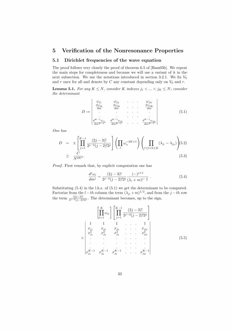
Lemma 5.1. For any K ≤ N , consider K indexes j1 < ... < jK ≤ N ; considerthe determinant
D :=
∣∣∣∣∣∣∣∣∣∣∣
ωj1 ωj2 . . . ωjKdωj1dm
dωj2dm . . .
dωjK
dm. . . . . .. . . . . .
dK−1ωj1dmK−1
dK−1ωj2dmK−1 . . .
dK−1ωjK
dmK−1
∣∣∣∣∣∣∣∣∣∣∣(5.1)
One has
D = ±
K−1∏j=1
(2j − 3)!2j−2(j − 2)!2j
(∏l
ω−2K+1il
) ∏1≤l<k≤K
(λjl − λjk)
(5.2)
≥ C
N2K2 . (5.3)
Proof. First remark that, by explicit computation one has
djωidmj
=(2j − 3)!
2j−2(j − 2)!2j(−)j+1
(λi +m)j−12. (5.4)
Substituting (5.4) in the l.h.s. of (5.1) we get the determinant to be computed.Factorize from the l− th column the term (λjl +m)1/2, and from the j− th rowthe term (2j−3)!
2j−2(j−2)!2j . The determinant becomes, up to the sign,
[K∏l=1
ωjl
]K−1∏j=1
(2j − 3)!2j−2(j − 2)!2j
×
∣∣∣∣∣∣∣∣∣∣∣∣∣∣
1 1 1 . . . 1xj1 xj2 xj3 . . . xjKx2j1
x2j2
x2j3
. . . x2jK
. . . . . . .
. . . . . . .
. . . . . . .
xK−1j1
xK−1j2
xK−1j3
. . . xK−1jK
∣∣∣∣∣∣∣∣∣∣∣∣∣∣(5.5)
33
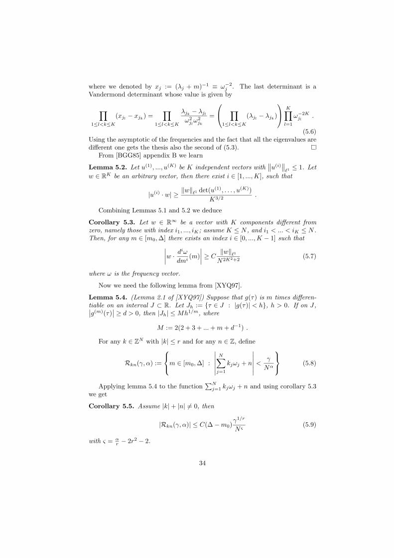
where we denoted by xj := (λj + m)−1 ≡ ω−2j . The last determinant is a
Vandermond determinant whose value is given by
∏1≤l<k≤K
(xjl − xjk) =∏
1≤l<k≤K
λjk − λjlω2jlω2jk
=
∏1≤l<k≤K
(λjl − λjk)
K∏l=1
ω−2Kjl
.
(5.6)Using the asymptotic of the frequencies and the fact that all the eigenvalues aredifferent one gets the thesis also the second of (5.3).
From [BGG85] appendix B we learn
Lemma 5.2. Let u(1), ..., u(K) be K independent vectors with∥∥u(i)
∥∥`1≤ 1. Let
w ∈ RK be an arbitrary vector, then there exist i ∈ [1, ...,K], such that
|u(i) · w| ≥‖w‖`1 det(u(1), . . . , u(K))
K3/2.
Combining Lemmas 5.1 and 5.2 we deduce
Corollary 5.3. Let w ∈ R∞ be a vector with K components different fromzero, namely those with index i1, ..., iK ; assume K ≤ N , and i1 < ... < iK ≤ N .Then, for any m ∈ [m0,∆] there exists an index i ∈ [0, ...,K − 1] such that∣∣∣∣w · diωdmi
(m)∣∣∣∣ ≥ C
‖w‖`1N2K2+2
(5.7)
where ω is the frequency vector.
Now we need the following lemma from [XYQ97].
Lemma 5.4. (Lemma 2.1 of [XYQ97]) Suppose that g(τ) is m times differen-tiable on an interval J ⊂ R. Let Jh := τ ∈ J : |g(τ)| < h, h > 0. If on J ,∣∣g(m)(τ)
∣∣ ≥ d > 0, then |Jh| ≤Mh1/m, where
M := 2(2 + 3 + ...+m+ d−1) .
For any k ∈ ZN with |k| ≤ r and for any n ∈ Z, define
Rkn(γ, α) :=
m ∈ [m0,∆] :
∣∣∣∣∣∣N∑j=1
kjωj + n
∣∣∣∣∣∣ < γ
Nα
(5.8)
Applying lemma 5.4 to the function∑Nj=1 kjωj + n and using corollary 5.3
we get
Corollary 5.5. Assume |k|+ |n| 6= 0, then
|Rkn(γ, α)| ≤ C(∆−m0)γ1/r
N ς(5.9)
with ς = αr − 2r2 − 2.
34
Lemma 5.6. Fix α > 2r3 + r2 + 5r. For any positive γ small enough thereexists a set Iγ ⊂ [m0,∆] such that ∀m ∈ Iγ one has that for any N ≥ 1∣∣∣∣∣∣
N∑j=1
kjωj + n
∣∣∣∣∣∣ ≥ γ
Nα(5.10)
for all k ∈ ZN with 0 6= |k| ≤ r and for all n ∈ Z. Moreover,
|[m0,∆]− Iγ | ≤ Cγ1/r . (5.11)
Proof. Define Iγ :=⋃nkRnk(γ, α). Remark that, from the asymptotic of the
frequencies, the argument of the modulus in (5.10) can be small only if |n| ≤CrN , By (5.9) one has∣∣∣∣∣⋃
k
Rnk(γ, α)
∣∣∣∣∣ ≤∑k
|Rk(γ, α)| < CNr(∆−m0)γ1/r
N ς,
summing over n one gets an extra factor rN . Provided α is chosen accordingto the statement, one has that the union over N is also bounded and thereforethe thesis holds.
Denote ω(N) := (ω1, ..., ωN ), then the statement of Theorem 3.12 is equiva-lent to
Lemma 5.7. For any γ positive and small enough, there exist a set Jγ satis-fying, |[m0,∆]− Jγ | → 0 when γ → 0, and a real number α′ such that for anym ∈ Jγ one has for N ≥ 1∣∣∣ω(N) · k + ε1ωj + ε2ωl
∣∣∣ ≥ γ
Nα′(5.12)
for any k ∈ ZN , εi = 0,±1, j ≥ l > N , and |k|+ |ε1|+ |ε2| 6= 0.
Proof. The case ε1 = ε2 = 0 reduces to the previous lemma with n = 0. Considerthe case ε1 = ±1 and ε2 = 0. In view of the asymptotic of the frequencies, theargument of the modulus can be small only if j < 2rN . Thus to obtain theresult one can simply apply lemma 5.6 with N ′ := 2rN in place of N andr′ := r + 2 in place of r. This just amounts to a redefinition of the constant Cin (5.11). The argument is identical in the case ε1ε2 = 1.
Consider now the case ε1ε2 = −1. Here the main remark is that
ωj − ωl = j − l + ajk with |ajl| ≤C
l(5.13)
So the quantity to be estimated reduces to
ω(N) · k ± n± ajl , n := j − l
If l > 2CNα/γ then the ajl term represent an irrelevant correction and thereforethe lemma follows from lemma 5.6. In the case l ≤ 2CNα/γ one reapplies thesame lemma with N ′ := 2CNα/γ in place of N and r′ := r+2 in place of r. Asa consequence one has that the nonresonance condition (5.12) holds providedα′ = α2 ∼ r6 and assuming that m is in a set whose complement has its measureestimated by a constant times γ
α+1r .
35
5.2 Periodic frequencies of the wave equation
We use the notations of section 3.2.2. We fix r and σ once for all and denoteby C any constant depending only on r and σ. We introduce τ0 = ω0 and forj ≥ 1,
γj := ωj − ω−j , τj =ωj + ω−j
2.
We recall that from the Sturm Liouville theory (cf. [KM01]) there exists anabsolute constant Cσ such that, for V ∈ VR,
|λj − λ−j | ≤ CσRe−2σj . (5.14)
We are going to prove the following result:
Theorem 5.8. Fix a positive r ≥ 2, define α := 200r3. There exists a positiveR and a positive b with the following property: for any γ > 0 small enough thereexists a set Sγ ⊂ VR and a constant β such that
i) For all V ∈ Sγ one has that for all N ≥ 1 the following inequality, withJ := b ln N
γβ , holds∣∣∣∣∣∣N∑j=1
τjkj +J∑j=1
γjnj +N∑
j=J+1
γj lj
∣∣∣∣∣∣ > γ
Nα(5.15)
for any k ∈ ZN+1, l ∈ ZN−J , n ∈ ZJ fulfilling |k| + |n| 6= 0, |k| + |l| +|n| ≤ r.
ii) |VR − Sγ | ≤ Cγ(1/4r).
Using arguments similar to those in the proof of lemma 5.7, one easily con-cludes that theorem 5.8 implies theorem 3.14.
The strategy of the proof of theorem 5.8 is as follow: when n = 0 (andthen k 6= 0) we only move the mass m in order to move the τj in such a waythat the l.h.s. of (5.15) is not too small. We also use that, for V ∈ VR, γj isexponentially small with respect to j and thus the third term in the l.h.s. of(5.15) is not relevant. In a second step we consider the case where n 6= 0 andwe use the Fourier coefficients vi to move the γj for small indexes j.
Fix k ∈ ZN , l ∈ ZN−J , n ∈ ZJ . For any α ∈ R and γ > 0 define
Sknl(γ, α) :=
(m, vk) ∈ VR :
∣∣∣∣∣∣N∑j=1
τjkj +J∑j=1
γjnj +N∑
j=J+1
γj lj
∣∣∣∣∣∣ ≤ γ
Nα
(5.16)
Lemma 5.9. For 0 6= |k| ≤ r
|Sk00(γ1, α1)| < Cγ
1/r1
N ς
with ς = α1r − 2r2 − 2.
36
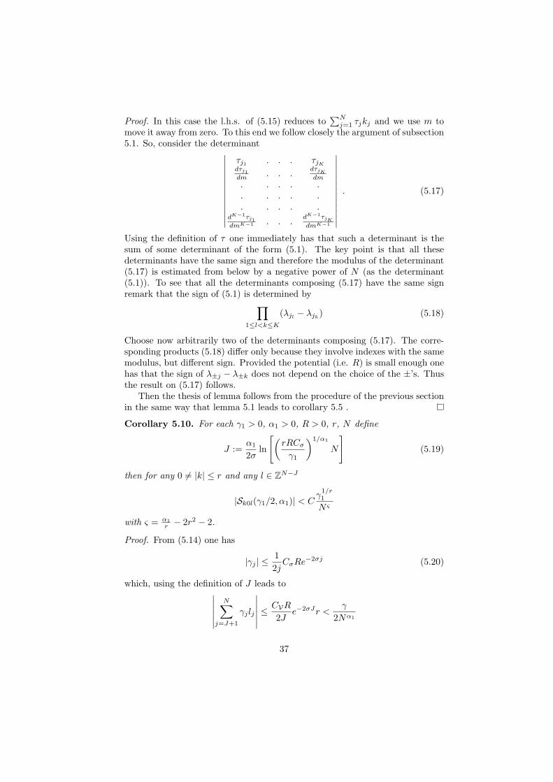
Proof. In this case the l.h.s. of (5.15) reduces to∑Nj=1 τjkj and we use m to
move it away from zero. To this end we follow closely the argument of subsection5.1. So, consider the determinant∣∣∣∣∣∣∣∣∣∣∣∣∣
τj1 . . . τjKdτj1dm . . .
dτjK
dm. . . . .. . . . .. . . . .
dK−1τj1dmK−1 . . .
dK−1τjK
dmK−1
∣∣∣∣∣∣∣∣∣∣∣∣∣. (5.17)
Using the definition of τ one immediately has that such a determinant is thesum of some determinant of the form (5.1). The key point is that all thesedeterminants have the same sign and therefore the modulus of the determinant(5.17) is estimated from below by a negative power of N (as the determinant(5.1)). To see that all the determinants composing (5.17) have the same signremark that the sign of (5.1) is determined by∏
1≤l<k≤K
(λjl − λjk) (5.18)
Choose now arbitrarily two of the determinants composing (5.17). The corre-sponding products (5.18) differ only because they involve indexes with the samemodulus, but different sign. Provided the potential (i.e. R) is small enough onehas that the sign of λ±j − λ±k does not depend on the choice of the ±’s. Thusthe result on (5.17) follows.
Then the thesis of lemma follows from the procedure of the previous sectionin the same way that lemma 5.1 leads to corollary 5.5 .
Corollary 5.10. For each γ1 > 0, α1 > 0, R > 0, r, N define
J :=α1
2σln
[(rRCσγ1
)1/α1
N
](5.19)
then for any 0 6= |k| ≤ r and any l ∈ ZN−J
|Sk0l(γ1/2, α1)| < Cγ
1/r1
N ς
with ς = α1r − 2r2 − 2.
Proof. From (5.14) one has
|γj | ≤12jCσRe
−2σj (5.20)
which, using the definition of J leads to∣∣∣∣∣∣N∑
j=J+1
γj lj
∣∣∣∣∣∣ ≤ CVR
2Je−2σJr <
γ
2Nα1
37
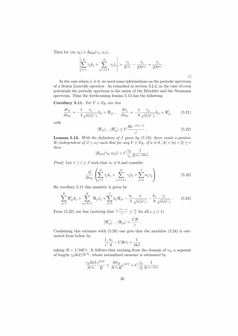
Then for (m, vk) ∈ Sk00(γ1, α1),∣∣∣∣∣∣N∑j=1
τjkj +N∑
j=J+1
γj lj
∣∣∣∣∣∣ > γ1
Nα1− γ1
2Nα1=
γ1
2Nα1.
In the case where n 6= 0, we need some informations on the periodic spectrumof a Sturm Liouville operator. As remarked in section 3.2.2, in the case of evenpotentials the periodic spectrum is the union of the Dirichlet and the Neumannspectrum. Thus the forthcoming lemma 5.13 has the following
Corollary 5.11. For V ∈ VR one has
∂γj∂v2i
= −14
τj√ωjω−j
δji +Rji ,∂τj∂v2i
= −18
γj√ωjω−j
δji +R′ji (5.21)
with
|Rji| , |R′ji| ≤ C
Re−σ|j−i|
j. (5.22)
Lemma 5.12. With the definition of J given by (5.19), there exists a positiveR (independent of J, γ, α) such that for any V ∈ VR, if n 6= 0, |k|+ |n|+ |l| ≤ rthen
|Sknl(γ2, α2)| < Cγ2
γ1
1Nα2−32α1
Proof. Let 1 ≤ i ≤ J such that ni 6= 0 and consider
∂
∂v2i
N∑j=1
τjkj +N∑
j=J+1
γj lj +J∑j=1
njγj
. (5.23)
By corollary 5.11 this quantity is given by
N∑j=1
R′jikj +
N∑j=J+1
Rjilj +J∑j=1
njRji −ni4
τi√ωiω−i
− ki8
γi√ωiω−i
. (5.24)
From (5.22) one has (noticing that e−σ|i−j|
j ≤ Ci for all i, j ≥ 1)∣∣R′
ji
∣∣ , |Rji| <CR
i.
Combining this estimate with (5.20) one gets that the modulus (5.24) is esti-mated from below by
1i(ni8− CRr) >
116J
taking R = 1/16Cr. It follows that excising from the domain of v2i a segmentof length γ216J/Nα2 , whose normalized measure is estimated by
γ216JNα2
e2Jσ
R≤ 16γ2
Nα2Re4Jσ = C
γ2
γ21
1Nα2−2α1
38
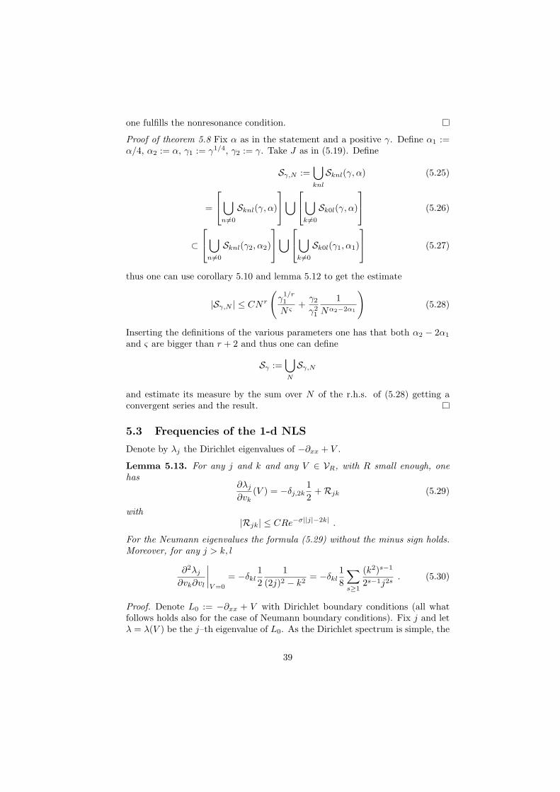
one fulfills the nonresonance condition.
Proof of theorem 5.8 Fix α as in the statement and a positive γ. Define α1 :=α/4, α2 := α, γ1 := γ1/4, γ2 := γ. Take J as in (5.19). Define
Sγ,N :=⋃knl
Sknl(γ, α) (5.25)
=
⋃n 6=0
Sknl(γ, α)
⋃⋃k 6=0
Sk0l(γ, α)
(5.26)
⊂
⋃n 6=0
Sknl(γ2, α2)
⋃⋃k 6=0
Sk0l(γ1, α1)
(5.27)
thus one can use corollary 5.10 and lemma 5.12 to get the estimate
|Sγ,N | ≤ CNr
(γ
1/r1
N ς+γ2
γ21
1Nα2−2α1
)(5.28)
Inserting the definitions of the various parameters one has that both α2 − 2α1
and ς are bigger than r + 2 and thus one can define
Sγ :=⋃N
Sγ,N
and estimate its measure by the sum over N of the r.h.s. of (5.28) getting aconvergent series and the result.
5.3 Frequencies of the 1-d NLS
Denote by λj the Dirichlet eigenvalues of −∂xx + V .
Lemma 5.13. For any j and k and any V ∈ VR, with R small enough, onehas
∂λj∂vk
(V ) = −δj,2k12
+Rjk (5.29)
with|Rjk| ≤ CRe−σ||j|−2k| .
For the Neumann eigenvalues the formula (5.29) without the minus sign holds.Moreover, for any j > k, l
∂2λj∂vk∂vl
∣∣∣∣V=0
= −δkl12
1(2j)2 − k2
= −δkl18
∑s≥1
(k2)s−1
2s−1j2s. (5.30)
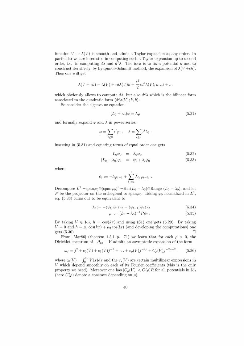
Proof. Denote L0 := −∂xx + V with Dirichlet boundary conditions (all whatfollows holds also for the case of Neumann boundary conditions). Fix j and letλ = λ(V ) be the j–th eigenvalue of L0. As the Dirichlet spectrum is simple, the
39
function V 7→ λ(V ) is smooth and admit a Taylor expansion at any order. Inparticular we are interested in computing such a Taylor expansion up to secondorder, i.e. in computing dλ and d2λ. The idea is to fix a potential h and toconstruct iteratively, by Lyapunof–Schmidt method, the expansion of λ(V +εh).Thus one will get
λ(V + εh) = λ(V ) + εdλ(V )h+ε2
2〈d2λ(V );h, h〉+ ...
which obviously allows to compute dλ, but also d2λ which is the bilinear formassociated to the quadratic form 〈d2λ(V );h, h〉.
So consider the eigenvalue equation
(L0 + εh)ϕ = λϕ (5.31)
and formally expand ϕ and λ in power series:
ϕ =∑l≥0
εlϕl , λ =∑l≥0
εlλl ,
inserting in (5.31) and equating terms of equal order one gets
L0ϕ0 = λ0ϕ0 (5.32)(L0 − λ0)ϕl = ψl + λlϕ0 (5.33)
where
ψl := −hϕl−1 +l∑
l0=1
λl0ϕl−l0 .
Decompose L2 =spanϕ0⊕(spanϕ0)⊥=Ker(L0 − λ0)⊕Range (L0 − λ0), and letP be the projector on the orthogonal to spanϕ0. Taking ϕ0 normalized in L2,eq. (5.33) turns out to be equivalent to
By taking V ∈ VR, h = cos(kx) and using (S1) one gets (5.29). By takingV = 0 and h = µ1 cos(kx) + µ2 cos(lx) (and developing the computations) onegets (5.30)
From [Mar86] (theorem 1.5.1 p. 71) we learn that for each ρ > 0, theDirichlet spectrum of −∂xx + V admits an asymptotic expansion of the form
0V (x)dx and the cs(V ) are certain multilinear expressions in
V which depend smoothly on each of its Fourier coefficients (this is the onlyproperty we need). Moreover one has |Cρ(V )| < C(ρ)R for all potentials in VR(here C(ρ) denote a constant depending on ρ).
40
Corollary 5.14.∂2cs∂vk∂vl
∣∣∣∣V=0
= δkl14k2(s−1)
2s. (5.37)
Proof. Just take the second derivative of equation (5.36) and compare with(5.30).
It follows that the ‘constants’ cs have an expansion at the origin of the form
cs(v1, v2, ...) =∑k≥1
Askv2k + ws(v1, v2, ...) (5.38)
where the matrix Ask is given by the r.h.s of (5.37) (without the Kroneckersymbol) and the functions ws have a zero of third order at the origin. Inparticular there exists for each k ≥ 1 a constant C(k) such that
|wk(v1, v2, ....)| ≤ C(k)R3 . (5.39)
Remark 5.15. For any ρ, the matrix
A := (Ask)s=1,...,ρk=1,...,ρ ,
is invertible and there exists a constant C that depends only on ρ such that∥∥A−1∥∥ ≤ C . (5.40)
(Indeed remark that the determinant of A is a non vanishing Vandermondedeterminant.)
In the remainder part of this section we fix once for all r ≥ 1. We beginwith the following simple lemma:
Lemma 5.16. Fix ρ ≥ l ≥ 1 two integers. For any J ≥ 2 and any positive µconsider an arbitrary collection of l indexes
J ≤ j1 < j2 < ... < jl ≤ Jµ , (5.41)
and define the matrix
B = (Bis)s=1,...,ρi=1,...,l , Bis :=
1j2si
. (5.42)
There exists an l × l submatrix Bl which is invertible and fulfills∥∥B−1l
∥∥ ≤ CJβ(µ,l) (5.43)
with β(µ, l) := 32µl(l − 1) and C ≡ C(l) is independent of J and of the choice
of the indexes.
41
Proof. Define the submatrix Bl = (Bis)s=1,...,li=1,...,l , notice that all the coefficients
of the comatrix of B are smaller than l2 and therefore∥∥B−1l
∥∥∞ ≤ l2(det Bl)−1 .
On the other hand, the determinant of Bl is a Vandermonde determinant whosevalue is given by ∏
1≤i<k≤l
(1j2i− 1j2k
) ∏1≤k≤l
1j2k
.
By the limitation (5.41) each term of the first product is estimated from belowby J−3µ. Since the number of pairs is l(l − 2)/4 one has the result.
Lemma 5.17. Given J ≥ 2 and µ > 1 consider an arbitrary collection ofindexes
J ≤ j1 < j2 < ... < jl ≤ Jµ , l ≤ r (5.44)
Let (aji)i=1,...,l be a vector with components in Z fulfilling
a 6= 0 ,∑i
|aji | ≤ r ,∑i
j2i aji = 0 . (5.45)
For any positive Γ and α > 2β(µ, l) define
R :=
V ∈ VR :
∣∣∣∣∣∑i
λjiaji
∣∣∣∣∣ ≤ ΓJα
. (5.46)
For R small enough, there exists two constants C1(r, α) and C2(r, α) such that,provided
J >C1
Γ1/2(5.47)
one has
|R| ≤ C2Γ1/2
Jα2−β
where β ≡ β(µ, l) is defined in the preceding lemma.
Proof. In order to fix ideas take l = r the other case being similar. Consider
∑i
λjiaji =r∑i=1
aji
ρ∑s=1
csj2si
+r∑i=1
ajiCρ(V )j2ρ+2i
The second term at r.h.s. is bounded by RrC(ρ)J2ρ+2 , thus if R ≤ 1, ρ = α/2 and
(5.47) is satisfied, it can be neglected and it remains to estimate the measure ofthe set of potentials such that∣∣∣∣∣
r∑i=1
aji
ρ∑s=1
csj2si
∣∣∣∣∣ < Γ2Jα
. (5.48)
42
We will show that there exists k ≤ ρ such that the second derivative of (5.48)with respect to vk is bounded away from zero, and we will apply lemma 5.4.One has
r∑i=1
aji
ρ∑s=1
csj2si
=r∑i=1
aji
ρ∑s=1
ρ∑k=1
Askv2k
j2si
+r∑i=1
aji
ρ∑s=1
wsj2si
+ b (5.49)
where
b :=r∑i=1
aji
ρ∑s=1
∑k>ρ
Askv2k
j2si
is independent of vk, k = 1, ..., ρ. Define wk by
ws =ρ∑k=1
Akswk ,
so that|wk| ≤ CR3
with a constant depending only on ρ (cf. (5.39) and (5.40)). So, (5.49) can bewritten as
ρ∑k=1
(v2k + wk)
ρ∑s=1
Aks
r∑i=1
Bijaji + b =ρ∑k=1
(v2k + wk)fk + b (5.50)
where B is given by (5.42) and fk is defined as the coefficient of the bracket atl.h.s. Clearly one has f = ABa. Now, the image of Rr under AB is an r dimen-sional space (due to remark 5.15 and lemma 5.16) and AB is an isomorphismbetween such r dimensional spaces. By remark 5.15 and lemma 5.16 its inverse(AB)−1 is bounded by ∥∥(AB)−1
∥∥ ≤ CJβ ,
(with C independent of J), and therefore one has
‖f‖ ≥ 1CJβ
‖a‖
It follows that there exists k with |fk| ≥ 1CJβ .
Consider now the second derivative of (5.50) with respect to vk, it is givenby
fk
(1 +
∂2wk∂v2
k
). (5.51)
Provided ∣∣∣∣∣∂2wk∂v2
k
∣∣∣∣∣ < 12
43
which is a smallness assumption on R (independent of J), (5.51) is larger than1
CJβ . Applying lemma 5.4 one gets the thesis.In the next lemme, we relax the hypothesis (5.44) of the previous lemma.
Lemma 5.18. There exists R and a positive constant C with the followingproperty: for any positive Γ there exists a set S1 ⊂ VR such that
i) denote α := 4r(r!)2, and let J be an integer fulfilling
J >C
Γ1/2(5.52)
then for any V ∈ S1 one has for N ≥ J∣∣∣∣∣r∑i=1
λjiaji
∣∣∣∣∣ ≥ ΓNα
(5.53)
for any choice of integers J ≤ j1, . . . , jr ≤ N and of relative integersajiri=1 fulfilling
0 6=∑i
|aji | ≤ r .
ii) S1 has large measure, namely
|VR − S1| ≤ CΓ1/2 (5.54)
Proof. We prove the lemma by induction on r. More precisely we prove thatfor any l ≤ r there exists a set Nl and two constants γl, α(l) such that∣∣∣∣∣
l∑i=1
λjiaji
∣∣∣∣∣ ≥ γlJα(l)
(5.55)
for any V ∈ Nl and moreover the measure estimate holds. The statement istrue for l = 1. Suppose it is true for l− 1, we prove it for l. Assume that all theintegers aj1 , ..., ajl are different from zero, otherwise the result follows by theinductive assumption. Order the indexes in increasing order. First remark thatif∑li=1 j
2i aji 6= 0 then
∣∣∣∑li=1 j
2i aji
∣∣∣ ≥ 1. Hence, since the potential is small (forR small enough) the l.h.s. of (5.55) is larger than 1/2 and the result holds inthis particular case. Thus we consider only the case where
∑li=1 j
2i aji = 0.
Now, since ∣∣λji − j2i∣∣ ≤ C
j2i,
if we assume that j2l >2rCJα(l−1)
γl−1, then we deduce from the inductive assumption
that ∣∣∣∣∣l∑i=1
λjiaji
∣∣∣∣∣ ≥∣∣∣∣∣l−1∑i=1
λjiaji
∣∣∣∣∣− rC
j2l≥ γl−1
2Jα(l−1).
44
and thus, provided γl ≤ γl−12 and αl ≥ αl−1, the lemma holds. So, assuming
J >C(r)
γ1/2l−1
, (5.56)
we have only to consider the case jl < Jµl where µl = [α(l − 1) + 2]/2.We now apply lemma 5.17. The number of possible choices for the integers
aj1 , . . . , ajl is smaller than J lµl .Therefore, the measure of the set of potentialsthat we have to exclude at the l-th step can be estimated by
Cγ1/2l J lµl
Jα(l)2 −β(µl,l)
Thus in order to obtain the result it suffices to choose αl in such way that
α(l) > α(l − 1)(3l2 + l)
which amounts to the requirement of a sufficiently fast growth of α(l). Thechoice α(l) = 4l(l!)2 fulfills this requirement. On the other hand, choosingγr = Γ, γl = γl−1/2 for l = 2, . . . , r and assuming (5.52) with a suitable constantC, (5.56) is satisfied for each l = 2, . . . , r. This gives the statement of the lemmawith a suitable constant in (5.54) and with J in place of N in (5.53). As J ≤ N ,the lemma is proved.
We now take into account the small indexes (j < J):
Lemma 5.19. There exists R > 0 with the following properties: for any γ > 0and J > 0 fulfilling
γe2σJ
R< 1 (5.57)
there exists a set SJ ⊂ VR∗ such that
i) ∀V ∈ SJ one has∣∣∣∣∣∣J∑j=1
λjkj +N∑
j=J+1
λjaj
∣∣∣∣∣∣ ≥ γ
Nr+2, ∀N ≥ J (5.58)
and for all k ∈ ZJ , a ∈ ZN−J fulfilling |k|+ |a| ≤ r, k 6= 0.
ii) |VR∗ − SJ | ≤γe2σJ
R.
Proof. To start with fix k and a. We estimate the measure of the set suchthat (5.58) is violated. Let i ≤ J such that ki 6= 0. Take the derivative ofthe argument of the modulus in (5.58) with respect to v2i. By (5.29) this isgiven by −1
2 ki + R with |R| < CR < 1/4 provided R is small enough. It hasto be remarked that, here, C does not depend on J, a, γ but only on r. Thusthe measure of the set such that (5.58) is violated for the given choice of (k, a)is estimated by γ
4Nr+2e2σJ
R . Summing over all the possible choices of k and a(namely Nr) and summing over N , one gets the thesis.
Combining the last two lemmas one gets
45
Theorem 5.20. Fix r ≥ 1 and α = 4r(r!)2. There exists R with the followingproperty: ∀γ > 0 there exists a set S ⊂ VR such that
i) for any V ∈ S one has for N ≥ 1∣∣∣∣∣∣N∑j=1
λjkj
∣∣∣∣∣∣ ≥ γ
Nα, (5.59)
for all k ∈ ZN with 0 6= |k| ≤ r.
ii) |VR − S| ≤[C ln
(R2
γ
)]−1/2
.
Proof. With a slight change of notation write (5.59) in the form∣∣∣∣∣∣J∑j=1
λjkj +N∑
j=J+1
λjaj
∣∣∣∣∣∣ ≥ γ
Nα(5.60)
with a still undetermined J . To begin with consider the case k = 0 and applylemma 5.18 with a still undetermined Γ. In order to fulfill (5.52) we choose nowJ := 2C
Γ1/2 . It follows that (5.60) holds for any γ ≤ Γ provided V belongs to aset S1 whose measure is estimated by CΓ1/2. If k 6= 0 then assuming
γe2σJ
R=γe
2σC
Γ1/2
R< 1
with R ≡ R(r) chosen as in lemma 5.19, one can apply lemma 5.19 and (5.60)is still satisfied.
Now we choose Γ in such a way that
γe2σC
Γ1/2
R= γ1/2
namely
Γ1/2 =4σC
ln(R2
γ ). (5.61)
It follows that γ < Γ and therefore (5.60) is true in SJ ∩S1, whose complementis estimated by twice the r.h.s. of (5.54) with Γ given by (5.61).
Finally, to deduce theorem 3.17 from theorem 5.20 just adapt the proof oflemma 5.7. To this end, instead of (5.13) use that, due to the asymptotic of thefrequencies, ωj − ωl > l/2.
5.4 Frequencies of coupled NLS
Denote ω(N) := (ω−N , ..., ωN ), then, by repeating the procedure of the previoussubsection, one gets the following
46
Theorem 5.21. Fix r ≥ 1 and α1 = 4r(r!)2. There exists R with the followingproperty: ∀γ1 > 0 there exists a set S ⊂ VR × VR such that
i) for any (V1, V2) ∈ S one has for N ≥ 1∣∣∣ω(N) · k∣∣∣ ≥ γ1
Nα1, (5.62)
for all k ∈ Z2N with 0 6= |k| ≤ r.
ii) |VR − S| ≤[C ln
(R2
γ1
)]−1/2
.
Proof of theorem 3.19. As in the proof of lemma 5.7 we study the inequality∣∣∣ω(N) · k + ε1ωj + ε2ωl
∣∣∣ ≥ γ
Nα(5.63)
with k ∈ Z2N , εi = 0,±1, |j| ≥ |l| > N . The cases ε1 = ε2 = 0 and ε1ε2 = 1 canbe treated exactly as in the proof of lemma 5.7; the same is true when ε1ε2 = −1and j and l have the same sign. In such cases one gets that (5.63) holds withα = 2α1 in a set whose complement is estimated by item ii of the theorem witha different constant C. Consider now the case ε1ε2 = −1, j > 0, l < 0. If j 6= −lthen the same argument as before applies. Take now l = −j and, to fix ideas,take ε1 = 1 and ε2 = −1, and write ω±j = ±j2 + ν±j with |ν±j | ≤ Cj−2. Thusthe argument of the modulus at l.h.s. of eq.(5.63) reduces to
ω(N) · k + νj − ν−j .
If j2 ≥ 2CNα1/γ1 then the ν terms can be neglected, and, provided k 6= 0 theestimate (5.63) follows. We have now to consider the case j2 < 2CNα1/γ1. Toget the estimate (5.63) simply apply (the procedure leading to) theorem 5.21with N substituted by 2CNα1/γ1. This leads to (5.63) with α = α2
1/2 andγ = Cγ
α1/2+11 .
5.5 Frequencies of NLS in higher dimension
Denote ω(N) := (ωj)|j|≤N .
Lemma 5.22. Fix r ≥ 1 and γ > 0 small enough. There exist positive constantsC ≡ Cr, β ≡ β(r, γ) and a set Sγ ⊂ V with |V −Sγ | → 0 when γ → 0 such that,if V ∈ Sγ then for any N ≥ 1 and any n ∈ Z
|ω(N) · k + n| ≥ γ
Nβ, (5.64)
for any k ∈ ZZd
with 0 < |k| ≤ r.
47
Proof. First of all recall that for V ∈ V, V (x) =∑k∈Zd vk e
ik·x, the frequenciesare given by
ωk = |k|2 + vk .
Then notice that, given (a1, . . . , ar) 6= 0 in Zr, M > 0 and c ∈ R the Lebesguemeasure of
x ∈ [−M,M ]r | |r∑i=1
aixi + c| < δ
is smaller than (2M)r−1δ. Hence given k ∈ ZZd
of length less than r and n ∈ Zthe Lebesgue measure of
Xk :=
x ∈ [−1/2, 1/2]Zd
:
∣∣∣∣∣∣∑|j|≤N
kj(|j|2 + xj) + n
∣∣∣∣∣∣ < γ
Nβ
is smaller than γ/Nβ . Therefore its probability measure is estimated by (1 +N)m(r−1)γ/RNβ . To conclude the proof we have to sum over all the k’s and theb’s. To count the cardinality of the set of the k’s and the n’s to be consideredremark that if |ω(N) ·k−n| ≥ δ with δ < 1 then |b| ≤ 1+|ω(N) ·k| ≤ 1+(1+N2)r.So that to ensure (5.64) for all possible choices of k, n and N , one has to removefrom V a set of measure∑
N≥1
γ1Nβ
(1 +N)m(r−1)(2N)dr(1 + (1 +N2)r) .
Choosing β := r(d+m)+5, the last series converges and the lemma is proved.
To deduce theorem 3.17 from lemma 5.22 one has just to adapt the proof oflemma 5.7.
A Technical Lemmas
A.1 Proof of lemma 4.11.
Introduce the projector Π on the modes with index smaller than N and theprojector Π on the modes with larger index. Expand f in Taylor series (in allthe variables), namely write
f =∑
j≤r∗+2
fj
with fj homogeneous of degree j. Consider the vector field of fj and decomposeit into the component on z and the component on z. One has:
ΠXfj = Jz∇zfj , (A.1)
ΠXfj = Jz∇zfj , (A.2)
48
where we denoted by Jz and Jz the two components of the Poisson tensor.From(A.1,A.2) one immediately realises that ΠXfj
has a zero of order three asa function of z and ΠXfj
has a zero of order two as a function of z. ConsiderΠXfj , write z = z + z, one has
ΠXfj(z + z) = ΠXfj
(z + z, ..., z + z︸ ︷︷ ︸(j−1)–times
) (A.3)
=j−1∑l=2
(j − 1l
)ΠXfj (z, ..., z︸ ︷︷ ︸
l–times
, z, ..., z︸ ︷︷ ︸(j−l−1)–times
)
where the sum starts from 2 since ΠXfjhas a zero of order two as a function
of z. We estimate now a single term of the sum. By the tame property we have∥∥∥∥∥∥∥ΠXfj(z, ..., z︸ ︷︷ ︸l–times
, z, ..., z︸ ︷︷ ︸(j−l−1)–times
)
∥∥∥∥∥∥∥s
(A.4)
≤ |Xfj |Ts1
j − 1
[l∑i=1
‖z‖l−11 ‖z‖s ‖z‖
j−1−l1 +
j−1∑i=l+1
‖z‖l1 ‖z‖s ‖z‖j−2−l1
]
Using the inequalities
‖z‖1 ≤‖z‖sNs−1
,
‖z‖s ≤ ‖z‖s , ‖z‖s ≤ ‖z‖s‖z‖1 ≤ ‖z‖s
which immediately follow from the definition of the norms one can estimate thequantity (A.4) by
1N (s−1)(l−1)
‖z‖j−1s
Inserting into (A.3) one gets for z ∈ Bs(R)∥∥∥ΠXfj(z)∥∥∥s≤ 2j−1 R
j−1
Ns−1|Xfj
|Ts .
A similar estimate with N2(s−1) instead of Ns−1 holds for ΠXfj(z). Therefore
∥∥Xfj (z)∥∥s≤ 2j
Rj−1
Ns−1|Xfj |Ts
and summing over j one gets the thesis.
49
A.2 Proof of lemma 4.12
One hasXf,g = [Xf , Xg] = dXfXg − dXgXf
Denote X := Xf , Y := Xg. Write
X(z) =∑
k,l1,...ln
X l1,...,lnk ekzl1 ...zln
and similarly for Y , then one has
b[X,Y ]e (z)
=∑
k,l1,...lnj1,...jm
∣∣∣nX l1,...,lnk Y j1,...,jmln
−mXl1,...,ln−1,jmln
Yj1,...,jm−1,lnk
∣∣∣ ekzl1 ...zln−1zj1 ...zjm
After symmetrization with respect to the indexes l1, ..., ln−1, j1, ..., jm, the quan-tities in the above modulus are the components of a multilinear symmetric form
˜b[X,Y ]e. Consider also the multilinear form with components obtained by sym-metrizing the quantities∑
ln
(∣∣∣nX l1,...,lnk Y j1,...,jmln
∣∣∣+ ∣∣∣mX l1,...,ln−1,jmln
Yj1,...,jm−1,lnk
∣∣∣) (A.5)
namely the form ˜d bXe bY e + ˜d bY e bXe. Let w = (z(1), ..., z(n+m−1)) be amultivector with all the vectors z(j) chosen in the positive octant (see remark
4.5). Then the value of ˜b[X,Y ]e on w is bounded by the value of ˜d bXe bY e +˜d bY e bXe on the same multivector and finally it suffices to estimate ˜d bXe bY e.The value of ˜d bXe bY e on the multivector w is given by
n∑σ
1(n+m− 1)!
bXe(z(σ(1)), ..., z(σ(n−1)), bY e(z(σ(n)), ..., z(σ(n+m−1)))
)(A.6)
where σ are here all the permutations of the first n+m− 1 integers.Consider one of the terms in the last sum, say the one corresponding to the
identical permutation. One has∥∥∥bXe(z(1), ..., z(n−1), bY e(z(n), ..., z(n+m−1)))∥∥∥
s≤ | bXe |Ts | bY e |Ts
n+m−1∑l=1
clyl ,
(A.7)where
yl :=∥∥∥z(1)
∥∥∥1...∥∥∥z(l−1)
∥∥∥1
∥∥∥z(l)∥∥∥s
∥∥∥z(l+1)∥∥∥
1...∥∥∥z(n+m−1)
∥∥∥1
and
cl :=1n, if l = 1, ..., n− 1
cl :=1mn
, if l = n, ..., n+m− 1 .
50
Now the important property is that∑l cl = 1. Consider now the norm of the
sum in (A.6), it is clear that it is again estimated by an expression of the formof the r.h.s. of (A.7) with suitable constants c′l. To compute the constants c′lremark that, due to the symmetry of the expression all the coefficients must beequals. Moreover, the symmetrization does not change the property that thesum of the coefficients is 1, and therefore one has c′l = 1/(n+m− 1) for all l’s.So, in conclusion one has∥∥∥ ˜d bXe bY e(w)
∥∥∥s≤ n| bXe |Ts | bY e |Ts ‖w‖s,1 ,
from which one gets the thesis.
B On the verification of the tame modulus prop-erty
It is clear that the linear combination of polynomials with tame modulus stillhas tame modulus. The tame modulus property is also stable by composition:
Lemma B.1. Let X : Ps → Ps and Y : Ps → Ps be two polynomial vector fieldswith s-tame modulus, then also their composition X Y has s-tame modulus.
Proof. Just remark that for any multivector w with all components in the pos-itive octant one has ∥∥∥ ˜bX Y e(w)
∥∥∥s≤∥∥∥ ˜bXe bY e(w)
∥∥∥s
and that the composition of tame maps is still a tame map, so that∥∥∥ ˜bX Y e(w)∥∥∥s≤ Cs ‖w‖1,s
with a suitable Cs.Now the idea is that if one is able to show that some elementary maps have
tame modulus(think of examples 2.9, 2.10), then the same is true for the mapsobtained by composing them.
We have already seen (cf example 2.4) that bounded linear maps are tame.Proposition B.2 below gives a simple condition to ensure that a linear map hastame modulus for all s ≥ 1. Such a condition will be very useful in studyingthe behaviour of the TM property under change of basis in Ps. In the followingproposition, given a linear operator A, we will consider its matrix defined byAz =
∑klAklzlek. We will simply write A = (Akl).
Proposition B.2. Let a be an injective and surjective map from Z to Z withthe property that there exists C > 0 such that
|l|C≤ |a(l)| ≤ C|l| (B.1)
51
and let A = (Akl) be a linear operator. If for any n there exists a constant Cnsuch that
|Akl| ≤Cn
(1 + |k − a(l)|)n(B.2)
then A has tame modulus.
Proof. First we get rid of the map a by reordering the basis in the space Psconstituting the domain of A. Namely we take as l-th element of the basis ea(l).This has the consequence of changing the norm in the domain; due to (B.1) thenew norm is equivalent to the old one. So we consider only the case where a isthe identity.
To prove that A has tame modulus it suffices to prove that |Akl| are thematrix elements of an operator which is bounded as an operator from Ps intoitself. This is clearly equivalent to the fact that Dkl := |Akl||k|s|l|−s is boundedfrom P0 into itself. Remark that, since
|k|(1 + |k − l|)|l|
≤ 1 ,
in view of (B.2), for any n there still exists a constant C ′n such that
Dkl ≤C ′n
(1 + |k − l|)n. (B.3)
Thus, using Schwartz inequality, one has
‖Dz‖20 =∑k
(∑l
Dklzl
)2
≤∑k
[(∑l
Dkl
)(∑l
Dklz2l
)]
= Kn
∑l
|zl|2(∑
k
Dkl
)= K2
n ‖z‖20
where we used the inequality (B.3) and we defined
Kn :=∑k
C ′n
(1 + |k − l|)n.
In the particular case of linear canonical maps one has
Proposition B.3. Let A(1)..., A(m) be linear operators fulfilling
|A(j)kl | ≤
Cn(1 + |k − aj(l)|)n
(B.4)
where the maps aj have the property (B.1). Let A := A(1) + ... + A(m) be acanonical map (which by the proposition B.2 has tame modulus) then also A−1
has tame modulus.
52
Proof. Denote by J the Poisson tensor, namely the operator z ≡ (pk, qk) 7→J(pk, qk) := (−qk, pk), which clearly has tame modulus. Then, by canonicityone has
A−1 = −JATJ = (−JA(1)TJ − ...− JA(m)TJ) .
But A(j)T still fulfills (B.4) with the roles of k and l exchanged, therefore it hastame modulus. It follows that the above expression has tame modulus.
Finally concerning changes of coordinates one has the following
Corollary B.4. Let z = Aw be a linear canonical transformation with the samestructure as in proposition B.3. If f ∈ T sM is a polynomial function with s-tamemodulus, then also the transformed function f A has s-tame modulus.
Proof. Just remark that XfA = A−1Xf A which is the composition of mapswith s-tame modulus.
Proof of theorem 3.6. First use the isomorphism (3.4) to identify Bs withPs. By hypothesis P has tame modulus in this basis. Then one has to pass tothe basis of the normal modes, namely to introduce the coordinates relative tothe basis ϕj . The matrix realizing the change of coordinates is canonical andhas the form (
B 00 B
)where the matrix elements of A are given by Bk,l = ϕkl . Therefore if (S1) issatisfied,
|Bk,l| ≤Cn
(1 + |k − l|)n+
Cn(1 + |k + l|)n
.
Thus, as a consequence of corollary B.2, one gets the thesis.
References
[Bam99] D. Bambusi, Nekhoroshev theorem for small amplitude solutions innonlinear Schrodinger equation, Math. Z. 130 (1999), 345–387.
[Bam03a] , An averaging theorem for quasilinear Hamiltonian PDEs,Ann. Henri Poincare 4 (2003), 685–712.
[Bam03b] , Birkhoff normal form for some nonlinear PDEs, Comm.Math. Physics 234 (2003), 253–283.
[Bam03c] , Birkhoff normal form for some quasilinear HamiltonianPDEs, Preprint (2003).
[BG03] D. Bambusi and B. Grebert, Forme normale pour NLS en dimensionquelconque, Compt. Rendu. Acad. Sciences Paris 337 (2003), 409–414.
53
[BGG85] G. Benettin, L. Galgani, and A. Giorgilli, A proof of Nekhoroshev’stheorem for the stability times in nearly integrable Hamiltonian sys-tems, Celestial Mech. 37 (1985), 1–25.
[Bou96] J. Bourgain, Construction of approximative and almost-periodic solu-tions of perturbed linear Schrodinger and wave equations, Geometricand Functional Analysis 6 (1996), 201–230.
[Bou00] , On diffusion in high-dimensional Hamiltonian systems andPDE, J. Anal. Math. 80 (2000), 1–35.
[Bou03] , Green function estimate for lattice Schrodinger operatorsand applications, Preprint (2003).
[Cra00] W. Craig, Problemes de petitts diviseurs dans les equationsaux derivees partielles, Panoramas et Syntheses, no. 9, SocieteMathematique de France, 2000.
[CW93] W. Craig and C. E. Wayne, Newton’s method and periodic solutionsof nonlinear wave equations, Comm. Pure Appl. Math. 46 (1993),1409–1498.
[Kla83] S. Klainerman, On ”almost global” solutions to quasilinear wave equa-tions in three space dimensions, Comm. Pure Appl. Math. 36 (1983),325–344.
[KM01] T. Kappeler and B. Mityagin, Estimates for periodic and Dirichleteigenvalues of the Schrodinger operator, SIAM J. Math. Anal. 33(2001), 113–152.
[KP03] T. Kappeler and J. Poschel, KAM & KdV, Springer, 2003.
[Kuk87] S. B. Kuksin, Hamiltonian perturbations of infinite-dimensional lin-ear systems with an imaginary spectrum, Funct. Anal. Appl. 21(1987), 192–205.
[Kuk00] , Analysis of Hamiltonian PDEs, Oxford University Press,Oxford, 2000.
[Mar86] V. Marchenko, Sturm-Liouville operators and applications,Birkhauser, Basel, 1986.
[Nik86] N.V. Nikolenko, The method of Poincare normal form in problems ofintegrability of equations of evolution type, Russ. Math. Surveys 41(1986), 63–114.
[PT87] J. Poschel and E. Trubowitz, Inverse spectral theory, Academic Press,Boston, 1987.
54
[Way90] C. E. Wayne, Periodic and quasi-periodic solutions of nonlinear waveequations via KAM theory, Comm. Math. Physics 127 (1990), 479–528.
[XYQ97] J. Xu, J. You, and Q. Qiu, Invariant tori for nearly integrable Hamil-tonian systems with degeneracy, Math. Z. 226 (1997), 375–387.
Benoit GrebertLaboratoire de Mathematique Jean Leray,Universite de Nantes,2, rue de la Houssiniere,44322 Nantes Cedex 3, FranceE-mail: [email protected]