Bit level diversity combining for D-MIMO Wenjing Lin Department of Electrical & Computer Engineering McGill University Montreal, Canada November 2011 A thesis submitted to McGill University in partial fulfillment of the requirements for the degree of Master of Engineering (M.Eng.) in Electrical Engineering c 2011 Wenjing Lin
Transcript
Bit level diversity combining for D-MIMO
Wenjing Lin
Department of Electrical & Computer Engineering
McGill UniversityMontreal, Canada
November 2011
A thesis submitted to McGill University in partial fulfillment of the requirements for the degreeof Master of Engineering (M.Eng.) in Electrical Engineering
Multiple-Input Multiple-Output (MIMO) transmission techniques have been shown to be a pow-erful performance enhancing technology in wireless communications. However in realistic sys-tems, when increasing the number of antennas in a restricted space, the capacity gain of MIMOis limited. Furthermore, co-located MIMO (C-MIMO) systems when affected by shadowing cannot improve link quality. This motivates us to investigate Distributed MIMO (D-MIMO) system.
This work considers a bit level combining scheme, aided by bit reliability information foran uplink D-MIMO system over a composite Rayleigh-lognormal fading channel. Bit reliabilityinformation is derived based on the logarithmic likelihood ratio (LLR) and further modified forthe MIMO detection schemes: SD-ML (Sphere Decoding - Maximum Likelihood) and MMSE-OSIC (Minimum Mean Square Error - Ordered Successive Interference Cancellation). Computersimulation results demonstrate that such bit level combining scheme provides significant per-formance improvements for D-MIMO with M transmit and L receive antennas on each of its Ngeographically dispersed receive node, over conventional C-MIMO with M transmit and L receiveantennas, even in the presence of channel estimation errors or channel spatial correlation. It isfound that such a D-MIMO system provides a comparable performance to a C-MIMO systemwith M transmit and NL receive antennas, especially when space correlation becomes significant.
Furthermore, an analytical BER evaluation technique is proposed for a C-MIMO systemwith SD-ML detection over a composite Rayleigh-lognormal fading channel with and withoutspatial correlation. Numerical results show that our technique provides tight approximations forC-MIMO over space uncorrelated, space semi-correlated and space correlated channels.
We also provide a theoretical BER approximation technique for a D-MIMO system withSD-ML detection over a composite Rayleigh-lognormal fading channel with and without spatialcorrelation. Numerical results show that by optimizing two parameters, the BER approximationtechinique provides good approximation for an uncorrelated D-MIMO when the number of trans-mit antennas equals the number of receive antennas on each of its N geographically dispersedreceive node. We further notice that these optimized parameters set for an uncorrelated D-MIMOwith equal number of transmit and receive antennas on each receive node can not provide goodapproximation for an uncorrelated D-MIMO when the number of transmit antennas is less thanthe number of receive antennas on each node. These analytical results confirm the significantperformance improvement provided by D-MIMO with bit level combining.
ii
Sommaire
Les techniques de transmission MIMO (Multiple-Input Multiple-Output) constituent une puis-sante technologie permettant des ameliorations significatives en termes de performance dans ledomaine des communications sans fil. Cependant, en pratique, lorsque le nombre d’antennes aug-mente dans un espace relativement restreint, le gain en capacite des systemes MIMO est limite.De plus, lorsqu’ils sont affectes par l’effet d’ombrage, les systemes MIMO co-localises (C-MIMO)ne peuvent ameliorer la qualite de transmission. Ces difficultes ont motive notre investigationdes systemes D-MIMO (Distributed-MIMO).
Cette these considere une methode de combinaison au niveau du bit, utilisant l’information surla fiabilite du bit, pour le canal montant d’un systeme D-MIMO subissant des evanouissementsde Rayleigh-lognormale. L’information sur la fiabilite du bit est etablie a partir de la fonctionde vraisemblance logarithmique (LLR) et est par la suite modifiee pour differentes methodesde detection pour les sysemes MIMO, incluant SD-ML (Sphere Decoding-Maximum Likelihood)et MMSE-OSIC (Minimum Mean Square Error-Ordered Successive Interference Cancellation).Les resultats des simulations par ordinateur demontrent que comparee a un C-MIMO conven-tionnel utilisant M antennes d’emission et L antennes de reception, la methode de combinaisonau niveau du bit fournit des ameliorations de performance significatives pour le D-MIMO util-isant M antennes d’emission et L antennes de reception sur chacun des N nœuds de receptiongeographiquement disperses, et ceci meme en presence d’erreurs d’estimation de canal ou decorrelation spatiale. Il est aussi demontre qu’un tel D-MIMO fournit une performance compa-rable a celle d’un C-MIMO avec M antennes d’emission et NL antennes de reception, surtoutlorsque la correlation spatiale est significative.
De plus, une technique d’evaluation analytique de la probabilite d’error est proposee pour unsysteme C-MIMO utilisant SD-ML comme methode de detection sur un canal a evanouissementscomposites de Rayleigh-lognormale avec ou sans correlation spatiale. Les resultats numeriquesmontrent que notre technique fournit de tres bonnes approximations pour un systeme C-MIMOavec ou sans correlation spatiale.
Nous presentons egalement une technique d’approximation theorique de la probabilite d’errorpour un systeme D-MIMO utilisant SD-ML comme methode de detection sur un canal a evanouis-sements composites de Rayleigh-lognormale avec ou sans correlation spatiale. Les resultatsnumeriques montrent qu’en optimisant deux parametres, notre technique d’approximation dela probabilite d’error fournit une bonne approximation pour le D-MIMO sans correlation spa-tiale utilisant M antennes d’emission et L antennes de reception sur chacun de ses N nœuds dereception geographiquement disperses. Cependant les valeurs optimales des parametres obtenuespour un D-MIMO ou le nombre d’antennes d’emission est egal au nombre d’antennes de receptiona chacun des nœuds de reception, ne peuvent fournir de bonnes approximations lorsque le nom-bre d’antennes d’emission est inferieur au nombre d’antennes de reception sur chacun des nœudsde reception. Ces resultats analytiques confirment l’amelioration significative de performancefournie par le D-MIMO utilisant la methode de combinaison au niveau du bit.
iii
Acknowledgments
First and foremost, I would like to thank my supervisor, Professor Harry Leib for his encour-agement and the technical instruction throughout my studies and research. He made greatcontribution to this thesis, he proposed the bit level combining algorithm at the Fusion Centerin D-MIMO and provided scheme for theoretical BER performance analysis of D-MIMO whichare significant parts in my research.
Secondly, I would like to thank all the labmates in wireless research lab for their fruitful helpand pleasant times. In particular I want to mention Mr. Djelili Radji who gave me a lot ofhelpful advice and provided the softwares for MIMO system with square QAM modulation forMMSE-OSIC and SD-ML detection schemes respectively, which are very important resourcesto my research. I also would like to send my gratitude to Mr. Djelili Radji for translating myAbstract into French.
Thirdly, I am grateful for Professor H. Leib for his financial support from his NSERC grants.Finally, I would like to thank my parents, my sister and my friends for their encouragement
and understanding doing my whole learning process.
5.1.1 PEP in case of spatial correlation at receiver . . . . . . . . . . . . . . . . . 555.1.2 PEP in case of no spatial correlation at receiver . . . . . . . . . . . . . . . 565.1.3 BER performance for C-MIMO over space uncorrelated channels . . . . . . 575.1.4 BER performance for C-MIMO over space correlated channels . . . . . . . 68
5.2 Performance Analysis for D-MIMO with SD-ML Detection . . . . . . . . . . . . . 1065.2.1 Computation of X(n)
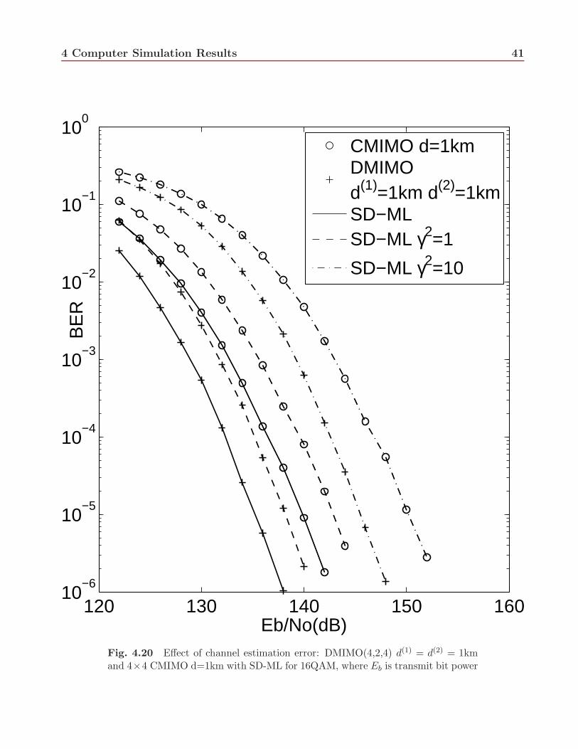
4.20 Effect of channel estimation error: DMIMO(4,2,4) d(1) = d(2) = 1km and 4 × 4CMIMO d=1km with SD-ML for 16QAM, where Eb is transmit bit power . . . . . 41
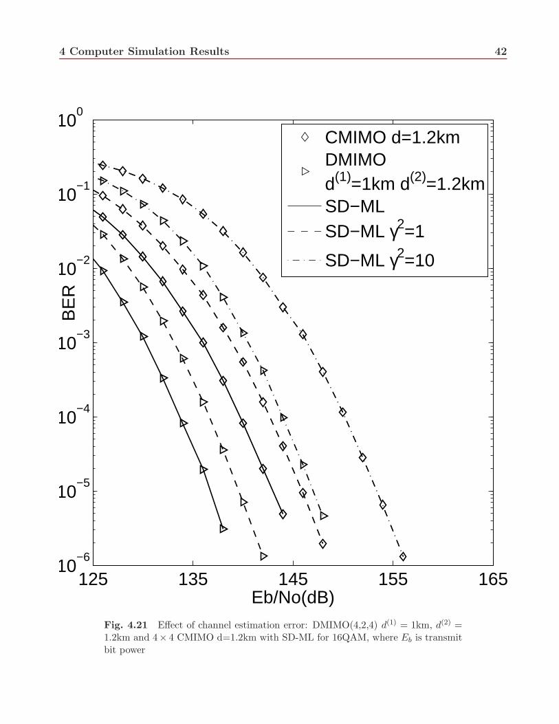
4.21 Effect of channel estimation error: DMIMO(4,2,4) d(1) = 1km, d(2) = 1.2km and4 × 4 CMIMO d=1.2km with SD-ML for 16QAM, where Eb is transmit bit power 42
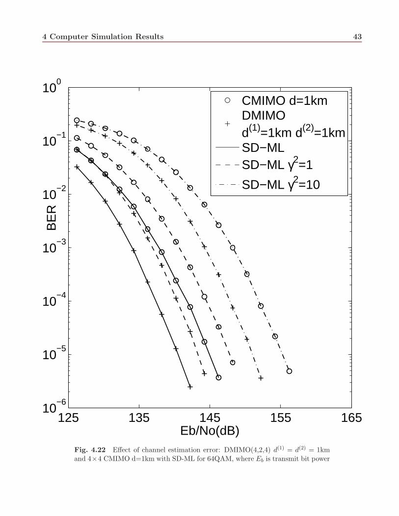
4.22 Effect of channel estimation error: DMIMO(4,2,4) d(1) = d(2) = 1km and 4 × 4CMIMO d=1km with SD-ML for 64QAM, where Eb is transmit bit power . . . . . 43
4.23 Effect of channel estimation error: DMIMO(4,2,4) d(1) = 1km, d(2) = 1.2km and4 × 4 CMIMO d=1.2km with SD-ML for 64QAM, where Eb is transmit bit power 44
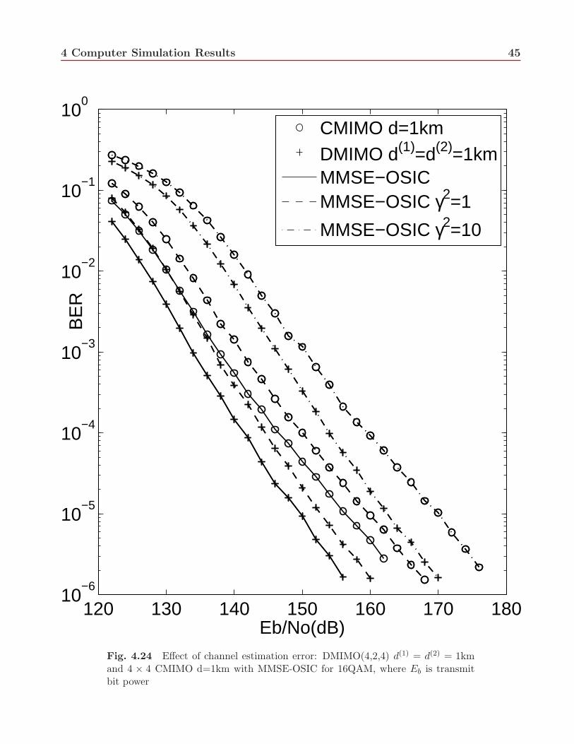
4.24 Effect of channel estimation error: DMIMO(4,2,4) d(1) = d(2) = 1km and 4 × 4CMIMO d=1km with MMSE-OSIC for 16QAM, where Eb is transmit bit power . 45
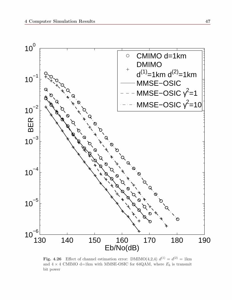
4.26 Effect of channel estimation error: DMIMO(4,2,4) d(1) = d(2) = 1km and 4 × 4CMIMO d=1km with MMSE-OSIC for 64QAM, where Eb is transmit bit power . 47
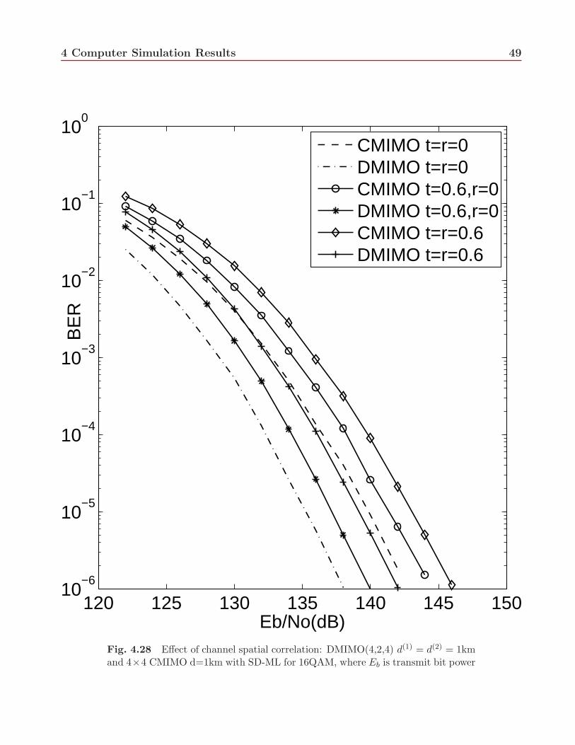
4.28 Effect of channel spatial correlation: DMIMO(4,2,4) d(1) = d(2) = 1km and 4 × 4CMIMO d=1km with SD-ML for 16QAM, where Eb is transmit bit power . . . . . 49
4.29 Effect of channel spatial correlation: DMIMO(4,2,4) d(1) = d(2) = 1km and 4 × 4CMIMO d=1km with SD-ML for 64QAM, where Eb is transmit bit power . . . . . 50
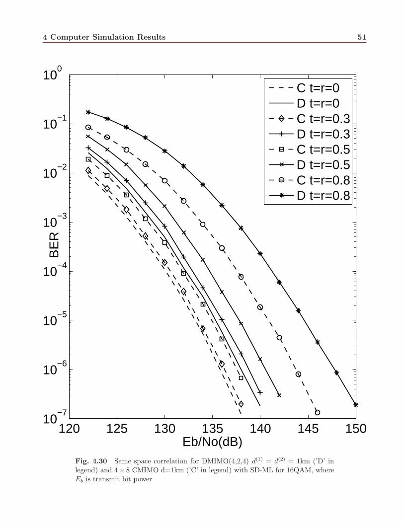
4.30 Same space correlation for DMIMO(4,2,4) d(1) = d(2) = 1km (’D’ in legend) and4×8 CMIMO d=1km (’C’ in legend) with SD-ML for 16QAM, where Eb is transmitbit power . . . . . . . . . . . . . . . . . . . . . . . . . . . . . . . . . . . . . . . . 51
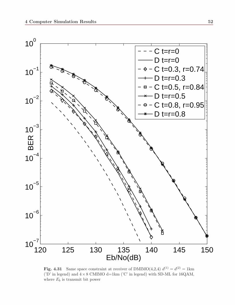
4.31 Same space constraint at receiver of DMIMO(4,2,4) d(1) = d(2) = 1km (’D’ inlegend) and 4×8 CMIMO d=1km (’C’ in legend) with SD-ML for 16QAM, whereEb is transmit bit power . . . . . . . . . . . . . . . . . . . . . . . . . . . . . . . . 52
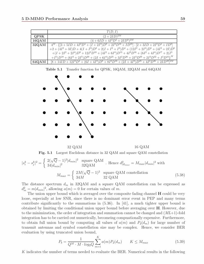
5.1 Largest Euclidean distance in 32 QAM and square QAM constellation . . . . . . . 595.2 BER evaluation for uncorrelated 2×2 C-MIMO with SD-ML for QPSK. Numbers
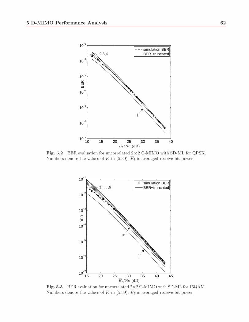
denote the values of K in (5.39), Eb is averaged receive bit power . . . . . . . . . 625.3 BER evaluation for uncorrelated 2×2 C-MIMO with SD-ML for 16QAM. Numbers
denote the values of K in (5.39), Eb is averaged receive bit power . . . . . . . . . 625.4 BER evaluation for uncorrelated 4×4 C-MIMO with SD-ML for QPSK. Numbers
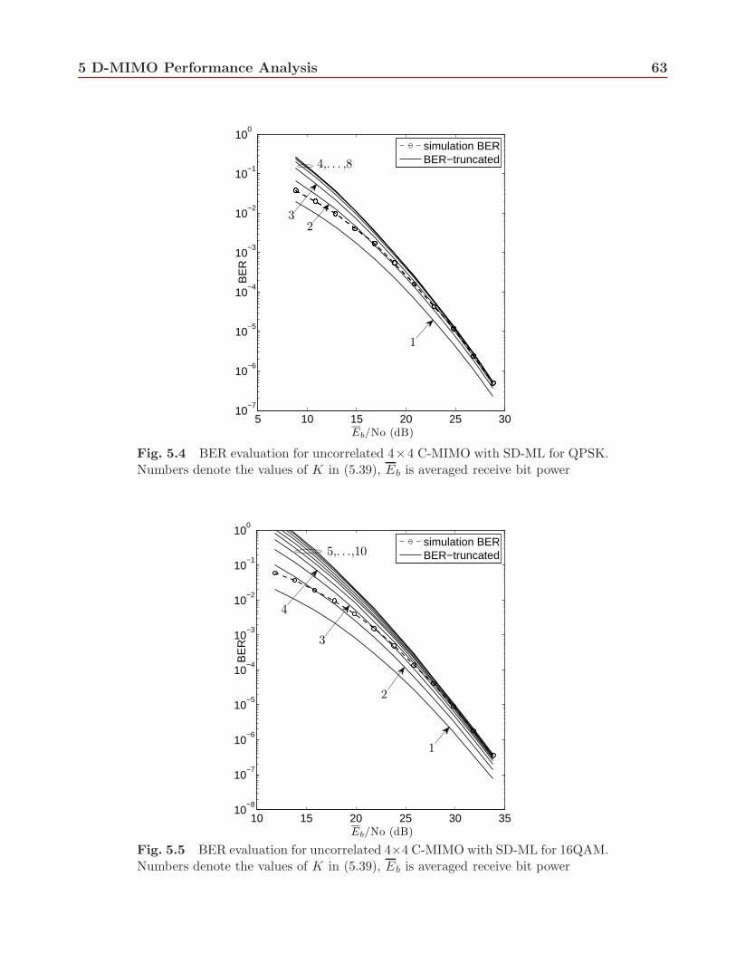
denote the values of K in (5.39), Eb is averaged receive bit power . . . . . . . . . 635.5 BER evaluation for uncorrelated 4×4 C-MIMO with SD-ML for 16QAM. Numbers
denote the values of K in (5.39), Eb is averaged receive bit power . . . . . . . . . 635.6 BER evaluation for uncorrelated 2×4 C-MIMO with SD-ML for QPSK. Numbers
denote the values of K in (5.39), Eb is averaged receive bit power . . . . . . . . . 64
List of Figures viii
5.7 BER evaluation for uncorrelated 2×4 C-MIMO with SD-ML for 16QAM. Numbersdenote the values of K in (5.39), Eb is averaged receive bit power . . . . . . . . . 64
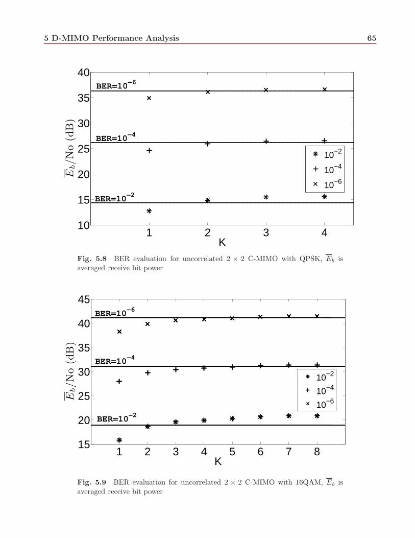
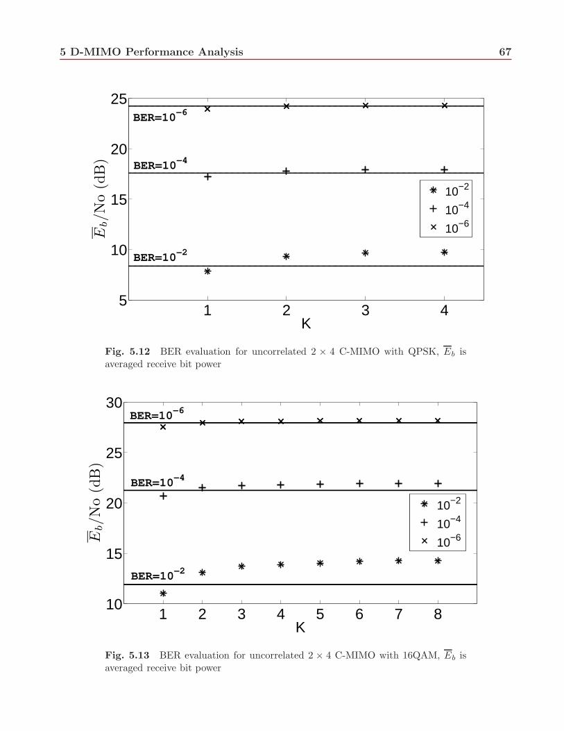
5.13 BER evaluation for uncorrelated 2 × 4 C-MIMO with 16QAM, Eb is averagedreceive bit power . . . . . . . . . . . . . . . . . . . . . . . . . . . . . . . . . . . . 67
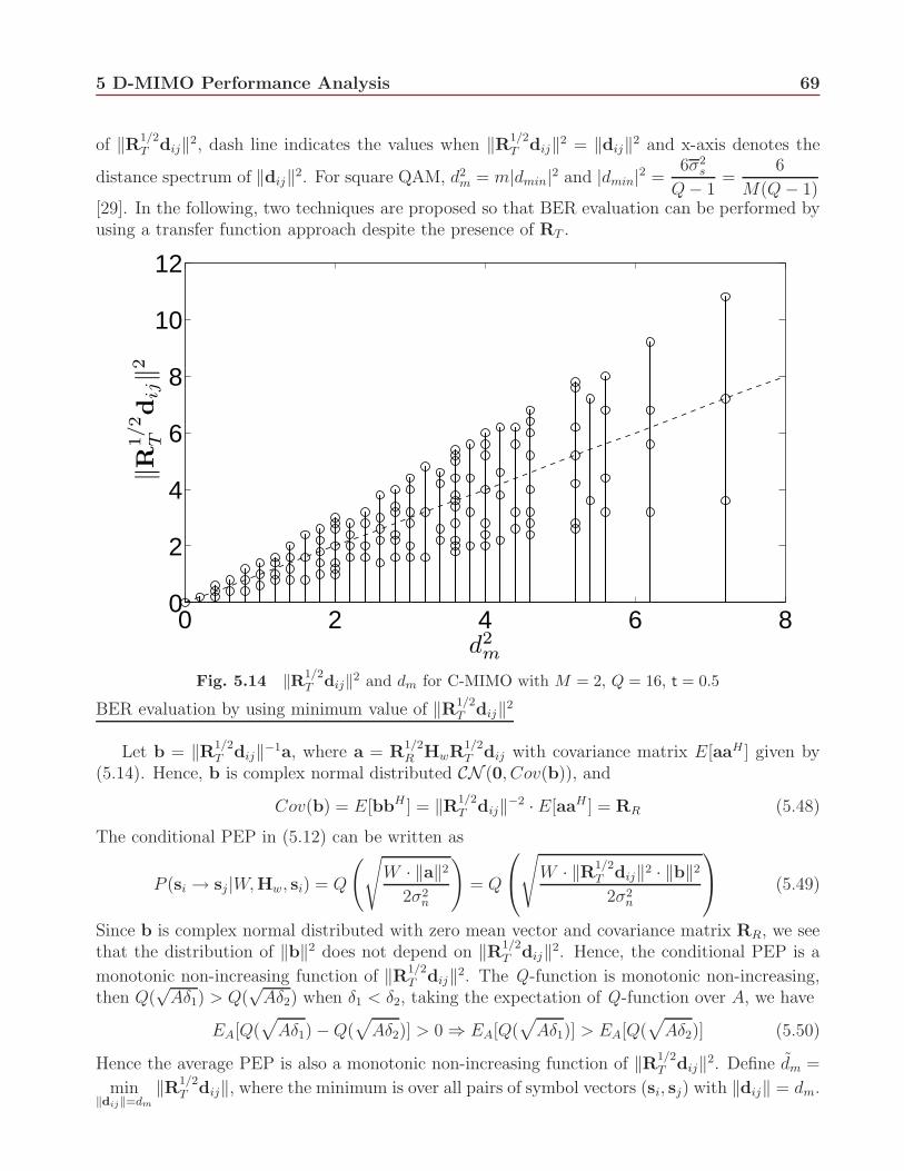
5.14 ‖R1/2T dij‖2 and dm for C-MIMO with M = 2, Q = 16, t = 0.5 . . . . . . . . . . . . 69
5.15 ‖R1/2T dij‖2 and dm for C-MIMO with M = 4, Q = 4, t = 0.5 . . . . . . . . . . . . 70
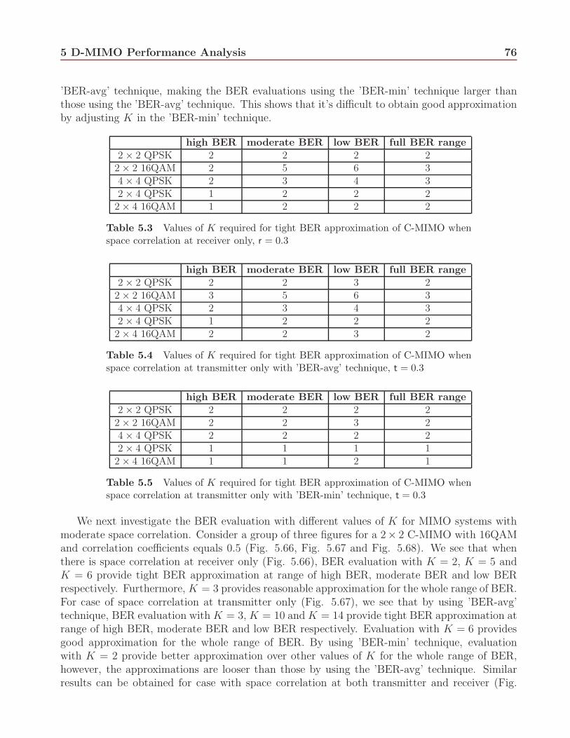
5.16 BER evaluation for 2× 2 C-MIMO with QPSK and r = 0.3. Numbers denote thevalues of K in (5.45), Eb is averaged receive bit power. . . . . . . . . . . . . . . . 78
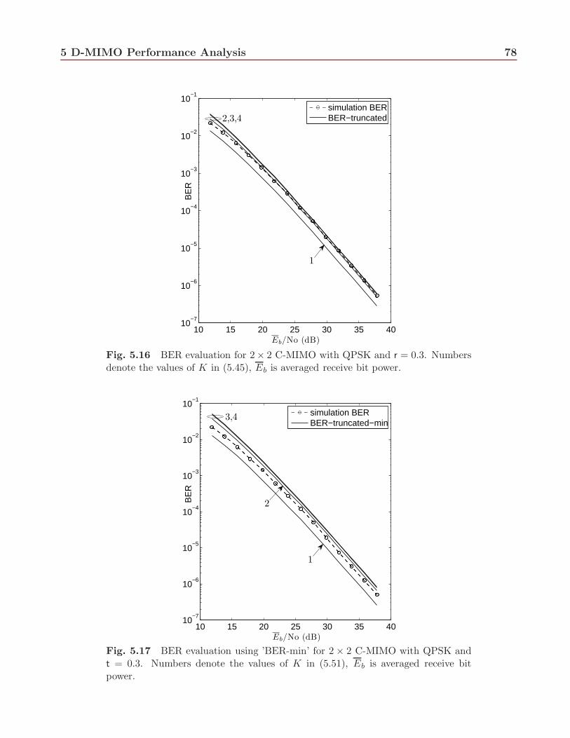
5.17 BER evaluation using ’BER-min’ for 2 × 2 C-MIMO with QPSK and t = 0.3.Numbers denote the values of K in (5.51), Eb is averaged receive bit power. . . . . 78
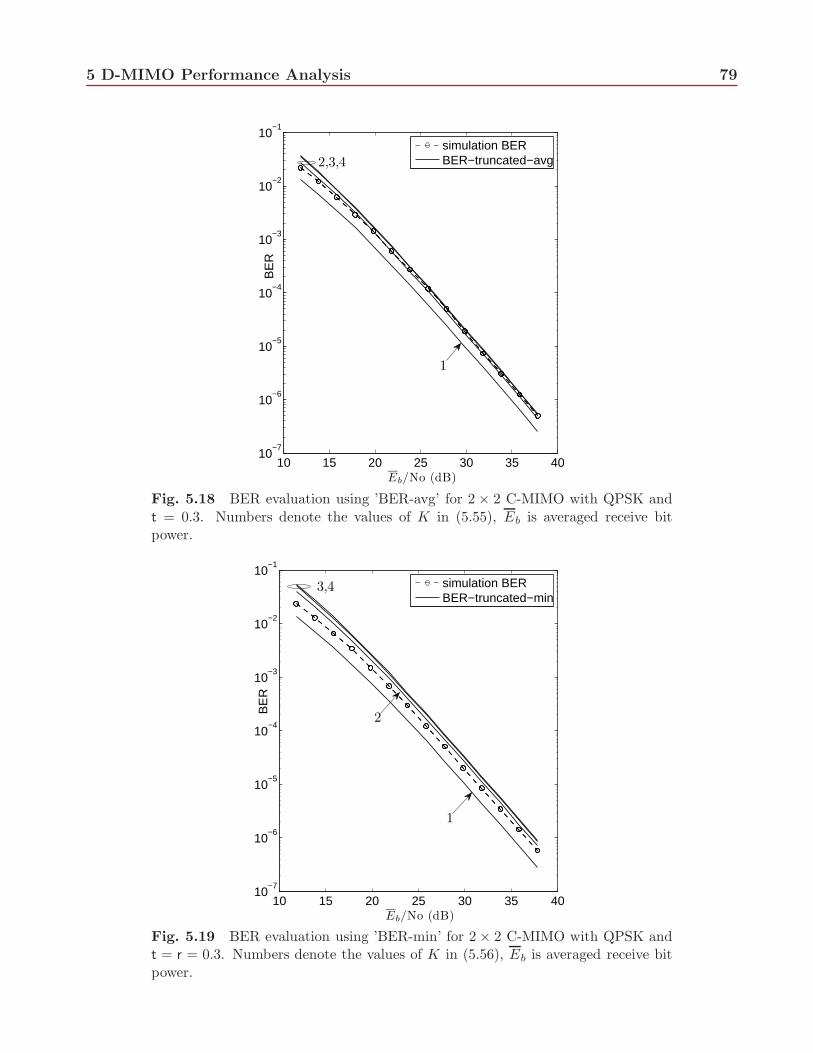
5.18 BER evaluation using ’BER-avg’ for 2 × 2 C-MIMO with QPSK and t = 0.3.Numbers denote the values of K in (5.55), Eb is averaged receive bit power. . . . . 79
5.19 BER evaluation using ’BER-min’ for 2× 2 C-MIMO with QPSK and t = r = 0.3.Numbers denote the values of K in (5.56), Eb is averaged receive bit power. . . . . 79
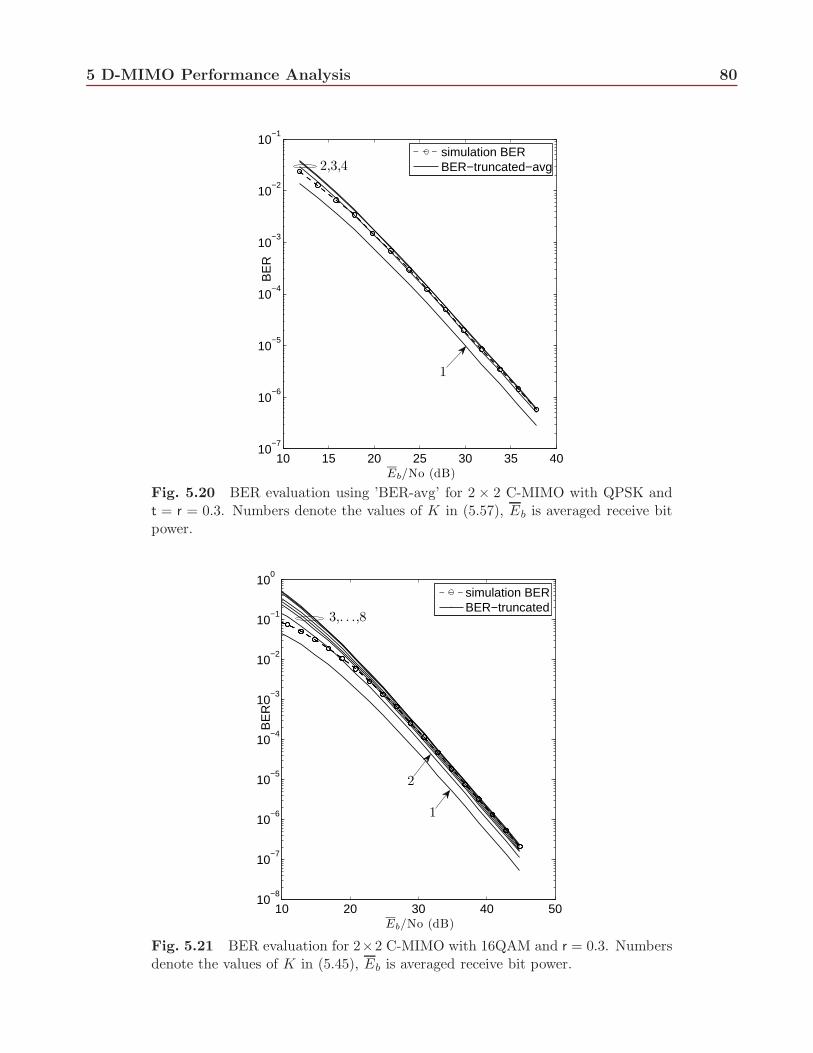
5.20 BER evaluation using ’BER-avg’ for 2 × 2 C-MIMO with QPSK and t = r = 0.3.Numbers denote the values of K in (5.57), Eb is averaged receive bit power. . . . . 80
5.21 BER evaluation for 2 × 2 C-MIMO with 16QAM and r = 0.3. Numbers denotethe values of K in (5.45), Eb is averaged receive bit power. . . . . . . . . . . . . . 80
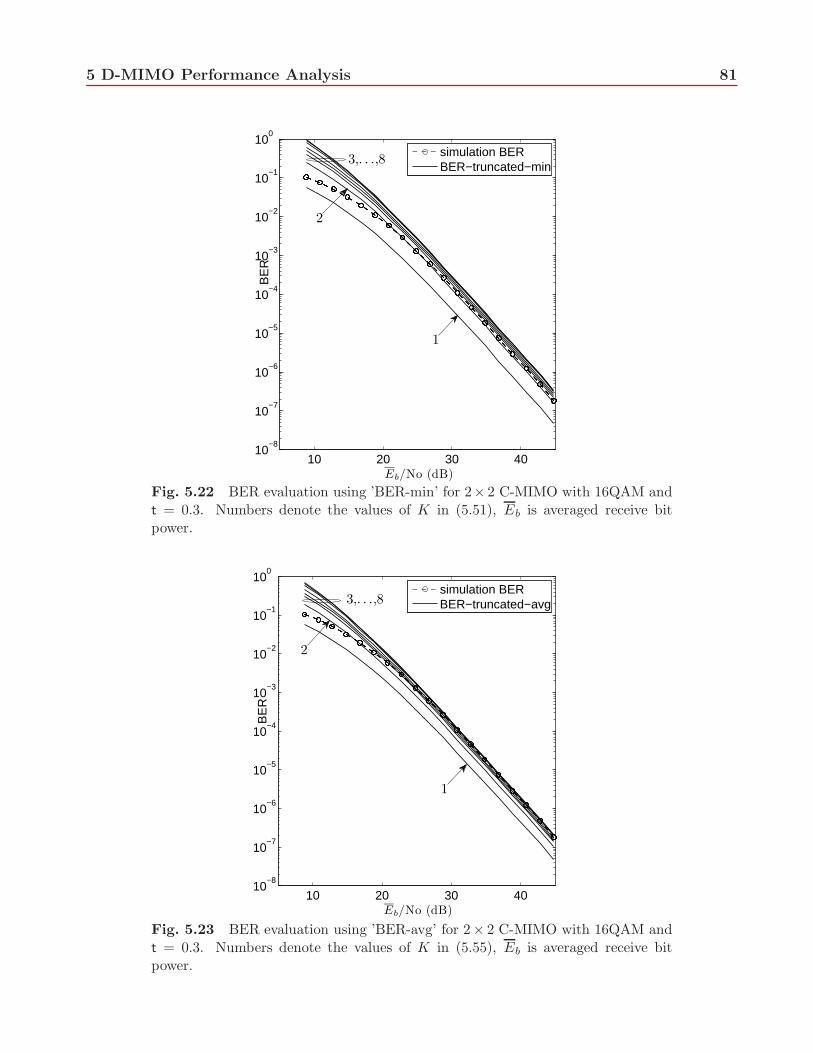
5.22 BER evaluation using ’BER-min’ for 2 × 2 C-MIMO with 16QAM and t = 0.3.Numbers denote the values of K in (5.51), Eb is averaged receive bit power. . . . . 81
5.23 BER evaluation using ’BER-avg’ for 2 × 2 C-MIMO with 16QAM and t = 0.3.Numbers denote the values of K in (5.55), Eb is averaged receive bit power. . . . . 81
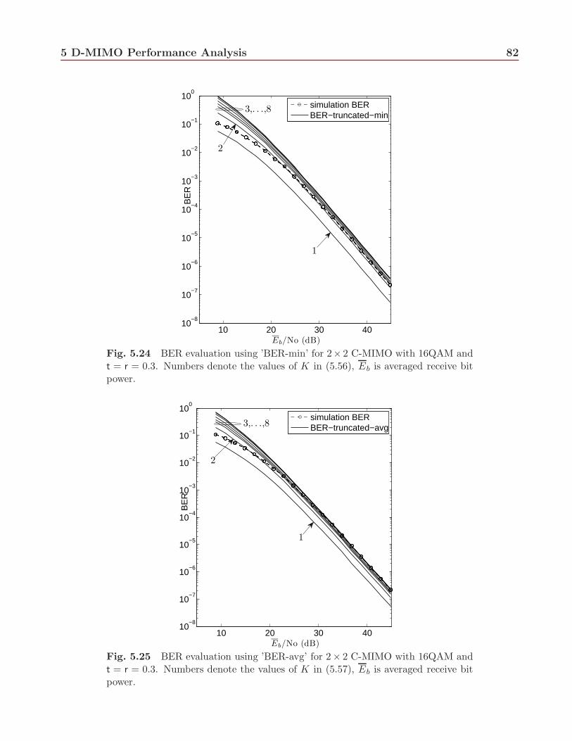
5.24 BER evaluation using ’BER-min’ for 2×2 C-MIMO with 16QAM and t = r = 0.3.Numbers denote the values of K in (5.56), Eb is averaged receive bit power. . . . . 82
5.25 BER evaluation using ’BER-avg’ for 2×2 C-MIMO with 16QAM and t = r = 0.3.Numbers denote the values of K in (5.57), Eb is averaged receive bit power. . . . . 82
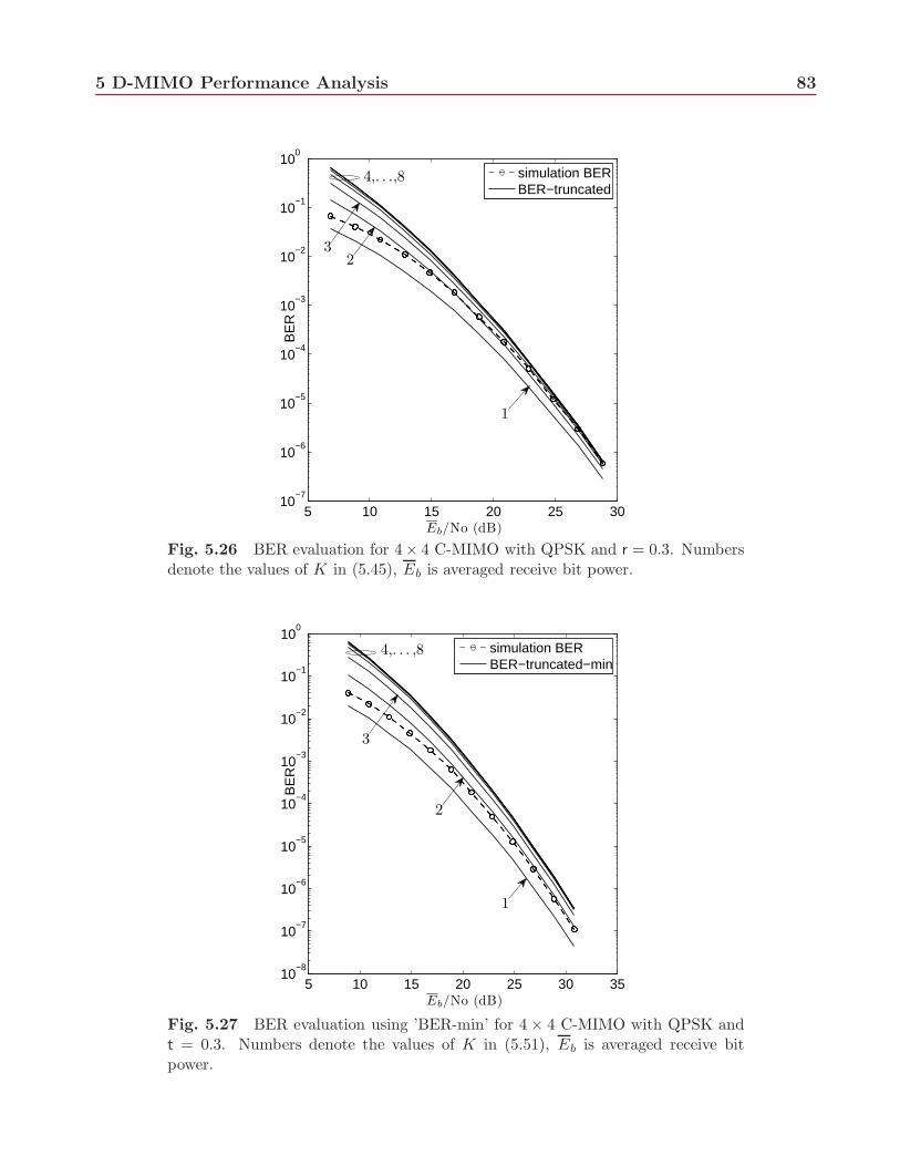
5.26 BER evaluation for 4× 4 C-MIMO with QPSK and r = 0.3. Numbers denote thevalues of K in (5.45), Eb is averaged receive bit power. . . . . . . . . . . . . . . . 83
5.27 BER evaluation using ’BER-min’ for 4 × 4 C-MIMO with QPSK and t = 0.3.Numbers denote the values of K in (5.51), Eb is averaged receive bit power. . . . . 83
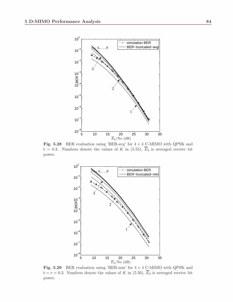
5.28 BER evaluation using ’BER-avg’ for 4 × 4 C-MIMO with QPSK and t = 0.3.Numbers denote the values of K in (5.55), Eb is averaged receive bit power. . . . . 84
5.29 BER evaluation using ’BER-min’ for 4× 4 C-MIMO with QPSK and t = r = 0.3.Numbers denote the values of K in (5.56), Eb is averaged receive bit power. . . . . 84
List of Figures ix
5.30 BER evaluation using ’BER-avg’ for 4 × 4 C-MIMO with QPSK and t = r = 0.3.Numbers denote the values of K in (5.57), Eb is averaged receive bit power. . . . . 85
5.31 BER evaluation for 2× 4 C-MIMO with QPSK and r = 0.3. Numbers denote thevalues of K in (5.45), Eb is averaged receive bit power . . . . . . . . . . . . . . . . 85
5.32 BER evaluation using ’BER-min’ for 2 × 4 C-MIMO with QPSK and t = 0.3.Numbers denote the values of K in (5.51), Eb is averaged receive bit power. . . . . 86
5.33 BER evaluation using ’BER-avg’ for 2 × 4 C-MIMO with QPSK and t = 0.3.Numbers denote the values of K in (5.55), Eb is averaged receive bit power. . . . . 86
5.34 BER evaluation using ’BER-min’ for 2× 4 C-MIMO with QPSK and t = r = 0.3.Numbers denote the values of K in (5.56), Eb is averaged receive bit power. . . . . 87
5.35 BER evaluation using ’BER-avg’ for 2 × 4 C-MIMO with QPSK and t = r = 0.3.Numbers denote the values of K in (5.57), Eb is averaged receive bit power. . . . . 87
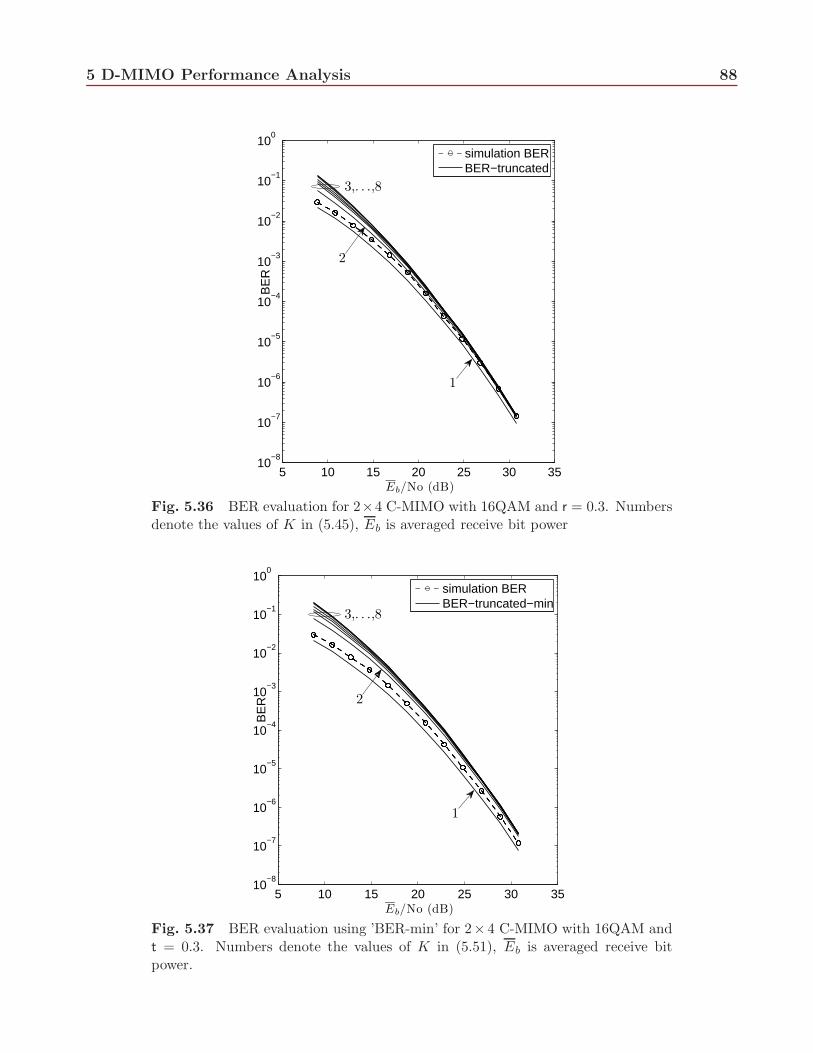
5.36 BER evaluation for 2 × 4 C-MIMO with 16QAM and r = 0.3. Numbers denotethe values of K in (5.45), Eb is averaged receive bit power . . . . . . . . . . . . . 88
5.37 BER evaluation using ’BER-min’ for 2 × 4 C-MIMO with 16QAM and t = 0.3.Numbers denote the values of K in (5.51), Eb is averaged receive bit power. . . . . 88
5.38 BER evaluation using ’BER-avg’ for 2 × 4 C-MIMO with 16QAM and t = 0.3.Numbers denote the values of K in (5.55), Eb is averaged receive bit power. . . . . 89
5.39 BER evaluation using ’BER-min’ for 2×4 C-MIMO with 16QAM and t = r = 0.3.Numbers denote the values of K in (5.56), Eb is averaged receive bit power. . . . . 89
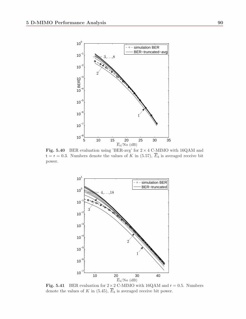
5.40 BER evaluation using ’BER-avg’ for 2×4 C-MIMO with 16QAM and t = r = 0.3.Numbers denote the values of K in (5.57), Eb is averaged receive bit power. . . . . 90
5.41 BER evaluation for 2 × 2 C-MIMO with 16QAM and r = 0.5. Numbers denotethe values of K in (5.45), Eb is averaged receive bit power. . . . . . . . . . . . . . 90
5.42 BER evaluation using ’BER-min’ for 2 × 2 C-MIMO with 16QAM and t = 0.5.Numbers denote the values of K in (5.51), Eb is averaged receive bit power. . . . . 91
5.43 BER evaluation using ’BER-avg’ for 2 × 2 C-MIMO with 16QAM and t = 0.5.Numbers denote the values of K in (5.55), Eb is averaged receive bit power. . . . . 91
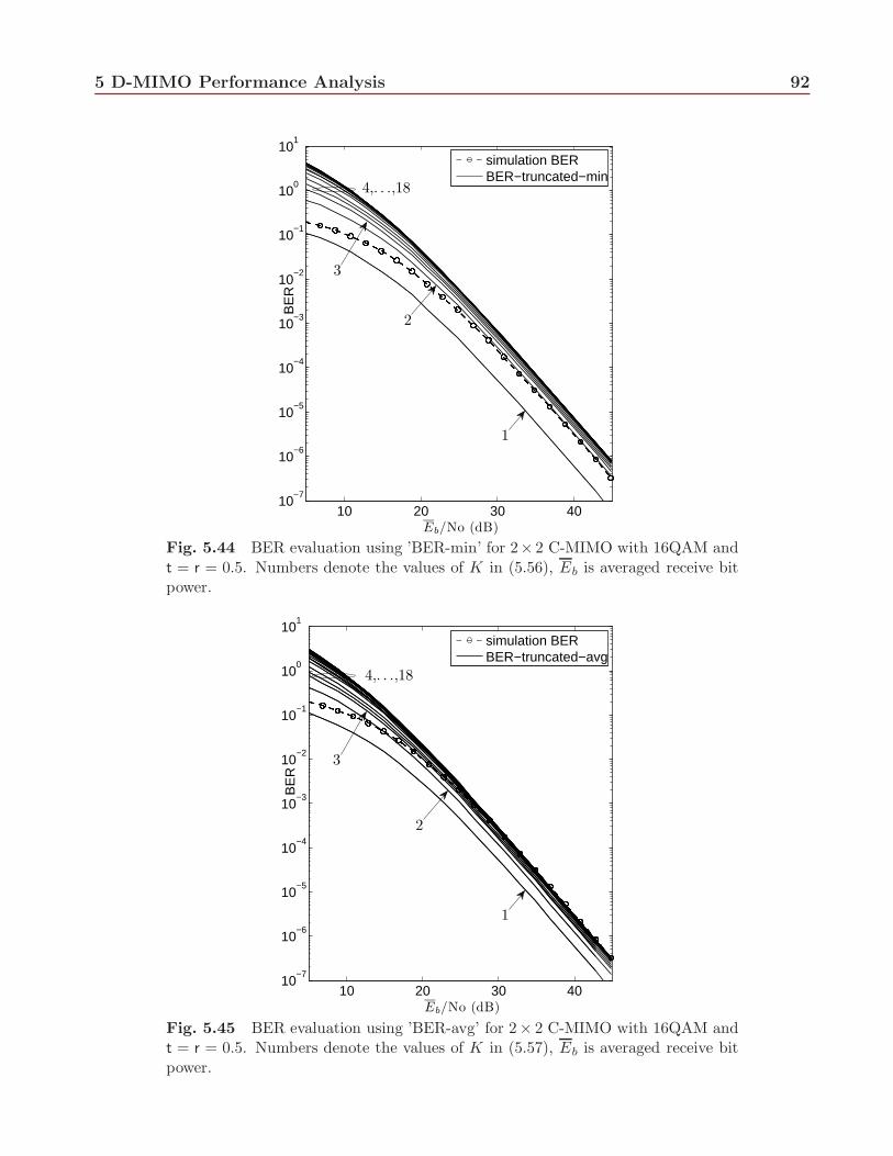
5.44 BER evaluation using ’BER-min’ for 2×2 C-MIMO with 16QAM and t = r = 0.5.Numbers denote the values of K in (5.56), Eb is averaged receive bit power. . . . . 92
5.45 BER evaluation using ’BER-avg’ for 2×2 C-MIMO with 16QAM and t = r = 0.5.Numbers denote the values of K in (5.57), Eb is averaged receive bit power. . . . . 92
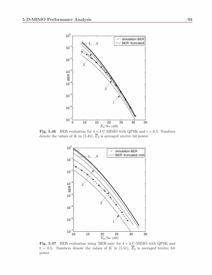
5.46 BER evaluation for 4× 4 C-MIMO with QPSK and r = 0.5. Numbers denote thevalues of K in (5.45), Eb is averaged receive bit power. . . . . . . . . . . . . . . . 93
5.47 BER evaluation using ’BER-min’ for 4 × 4 C-MIMO with QPSK and t = 0.5.Numbers denote the values of K in (5.51), Eb is averaged receive bit power. . . . . 93
5.48 BER evaluation using ’BER-avg’ for 4 × 4 C-MIMO with QPSK and t = 0.5.Numbers denote the values of K in (5.55), Eb is averaged receive bit power. . . . . 94
5.49 BER evaluation using ’BER-min’ for 4× 4 C-MIMO with QPSK and t = r = 0.5.Numbers denote the values of K in (5.56), Eb is averaged receive bit power. . . . . 94
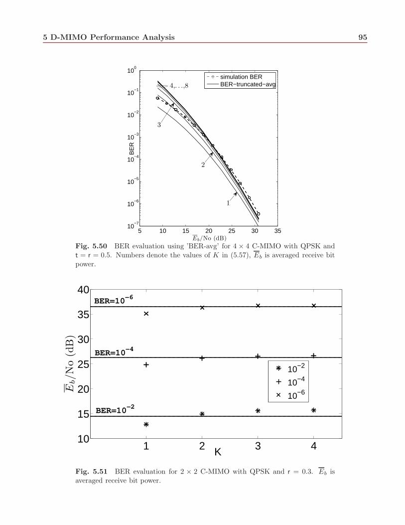
5.50 BER evaluation using ’BER-avg’ for 4 × 4 C-MIMO with QPSK and t = r = 0.5.Numbers denote the values of K in (5.57), Eb is averaged receive bit power. . . . . 95
5.51 BER evaluation for 2×2 C-MIMO with QPSK and r = 0.3. Eb is averaged receivebit power. . . . . . . . . . . . . . . . . . . . . . . . . . . . . . . . . . . . . . . . . 95
List of Figures x
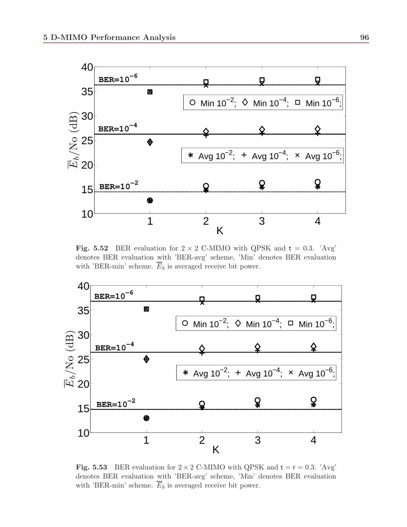
5.52 BER evaluation for 2 × 2 C-MIMO with QPSK and t = 0.3. ’Avg’ denotes BERevaluation with ’BER-avg’ scheme, ’Min’ denotes BER evaluation with ’BER-min’scheme. Eb is averaged receive bit power. . . . . . . . . . . . . . . . . . . . . . . . 96
5.53 BER evaluation for 2×2 C-MIMO with QPSK and t = r = 0.3. ’Avg’ denotes BERevaluation with ’BER-avg’ scheme, ’Min’ denotes BER evaluation with ’BER-min’scheme. Eb is averaged receive bit power. . . . . . . . . . . . . . . . . . . . . . . . 96
5.54 BER evaluation for 2 × 2 C-MIMO with 16QAM and r = 0.3. Eb is averagedreceive bit power. . . . . . . . . . . . . . . . . . . . . . . . . . . . . . . . . . . . . 97
5.55 BER evaluation for 2× 2 C-MIMO with 16QAM and t = 0.3. ’Avg’ denotes BERevaluation with ’BER-avg’ scheme, ’Min’ denotes BER evaluation with ’BER-min’scheme. Eb is averaged receive bit power. . . . . . . . . . . . . . . . . . . . . . . . 97
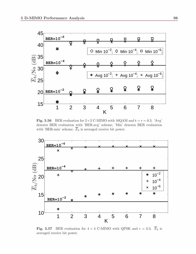
5.56 BER evaluation for 2 × 2 C-MIMO with 16QAM and t = r = 0.3. ’Avg’ de-notes BER evaluation with ’BER-avg’ scheme, ’Min’ denotes BER evaluation with’BER-min’ scheme. Eb is averaged receive bit power. . . . . . . . . . . . . . . . . 98
5.57 BER evaluation for 4×4 C-MIMO with QPSK and r = 0.3. Eb is averaged receivebit power. . . . . . . . . . . . . . . . . . . . . . . . . . . . . . . . . . . . . . . . . 98
5.58 BER evaluation for 4 × 4 C-MIMO with QPSK and t = 0.3. ’Avg’ denotes BERevaluation with ’BER-avg’ scheme, ’Min’ denotes BER evaluation with ’BER-min’scheme. Eb is averaged receive bit power. . . . . . . . . . . . . . . . . . . . . . . . 99
5.59 BER evaluation for 4×4 C-MIMO with QPSK and t = r = 0.3. ’Avg’ denotes BERevaluation with ’BER-avg’ scheme, ’Min’ denotes BER evaluation with ’BER-min’scheme. Eb is averaged receive bit power. . . . . . . . . . . . . . . . . . . . . . . . 99
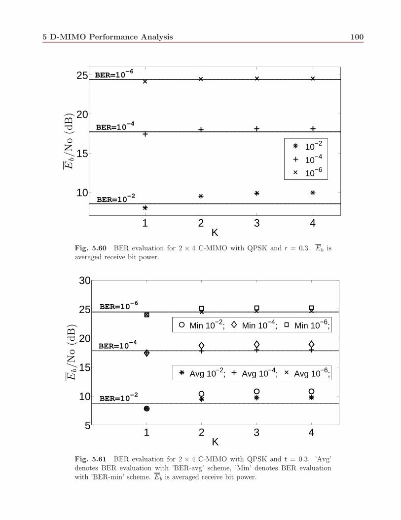
5.60 BER evaluation for 2×4 C-MIMO with QPSK and r = 0.3. Eb is averaged receivebit power. . . . . . . . . . . . . . . . . . . . . . . . . . . . . . . . . . . . . . . . . 100
5.61 BER evaluation for 2 × 4 C-MIMO with QPSK and t = 0.3. ’Avg’ denotes BERevaluation with ’BER-avg’ scheme, ’Min’ denotes BER evaluation with ’BER-min’scheme. Eb is averaged receive bit power. . . . . . . . . . . . . . . . . . . . . . . . 100
5.62 BER evaluation for 2×4 C-MIMO with QPSK and t = r = 0.3. ’Avg’ denotes BERevaluation with ’BER-avg’ scheme, ’Min’ denotes BER evaluation with ’BER-min’scheme. Eb is averaged receive bit power. . . . . . . . . . . . . . . . . . . . . . . . 101
5.63 BER evaluation for 2 × 4 C-MIMO with 16QAM and r = 0.3. Eb is averagedreceive bit power. . . . . . . . . . . . . . . . . . . . . . . . . . . . . . . . . . . . . 101
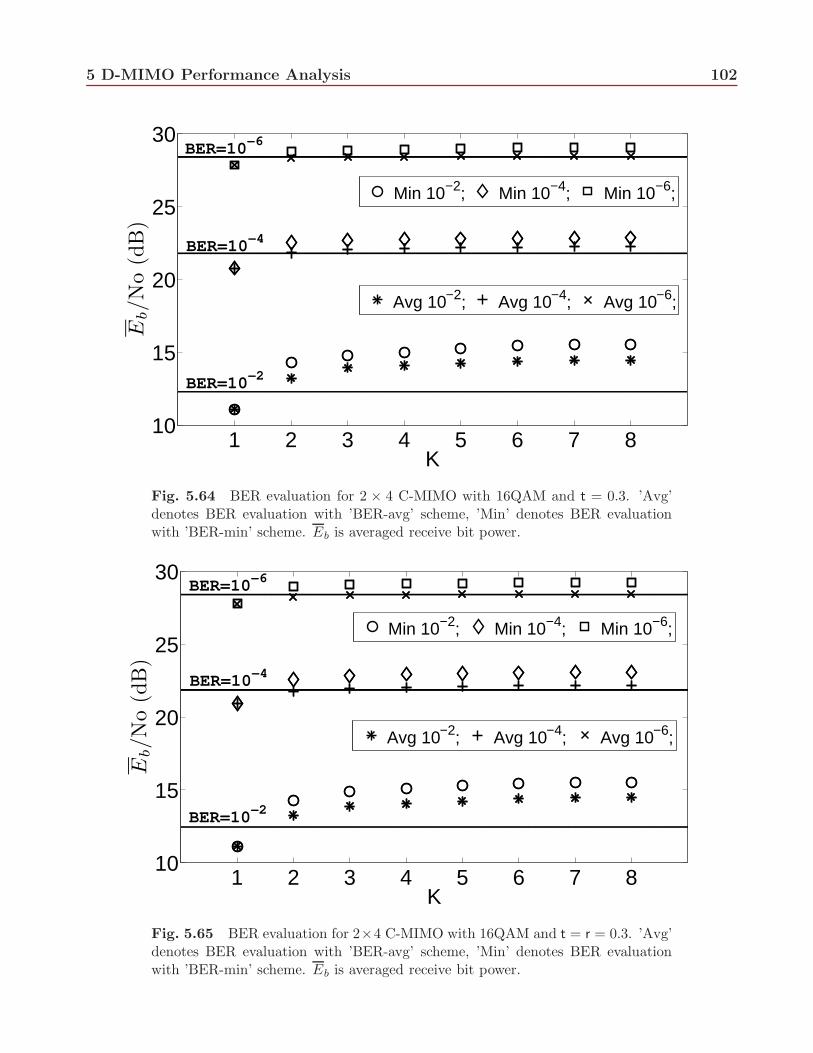
5.64 BER evaluation for 2× 4 C-MIMO with 16QAM and t = 0.3. ’Avg’ denotes BERevaluation with ’BER-avg’ scheme, ’Min’ denotes BER evaluation with ’BER-min’scheme. Eb is averaged receive bit power. . . . . . . . . . . . . . . . . . . . . . . . 102
5.65 BER evaluation for 2 × 4 C-MIMO with 16QAM and t = r = 0.3. ’Avg’ de-notes BER evaluation with ’BER-avg’ scheme, ’Min’ denotes BER evaluation with’BER-min’ scheme. Eb is averaged receive bit power. . . . . . . . . . . . . . . . . 102
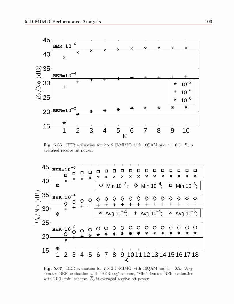
5.66 BER evaluation for 2 × 2 C-MIMO with 16QAM and r = 0.5. Eb is averagedreceive bit power. . . . . . . . . . . . . . . . . . . . . . . . . . . . . . . . . . . . . 103
5.67 BER evaluation for 2× 2 C-MIMO with 16QAM and t = 0.5. ’Avg’ denotes BERevaluation with ’BER-avg’ scheme, ’Min’ denotes BER evaluation with ’BER-min’scheme. Eb is averaged receive bit power. . . . . . . . . . . . . . . . . . . . . . . . 103
List of Figures xi
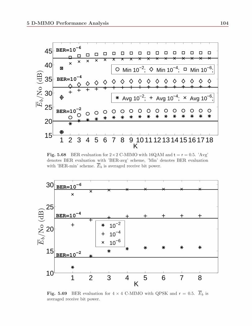
5.68 BER evaluation for 2 × 2 C-MIMO with 16QAM and t = r = 0.5. ’Avg’ de-notes BER evaluation with ’BER-avg’ scheme, ’Min’ denotes BER evaluation with’BER-min’ scheme. Eb is averaged receive bit power. . . . . . . . . . . . . . . . . 104
5.69 BER evaluation for 4×4 C-MIMO with QPSK and r = 0.5. Eb is averaged receivebit power. . . . . . . . . . . . . . . . . . . . . . . . . . . . . . . . . . . . . . . . . 104
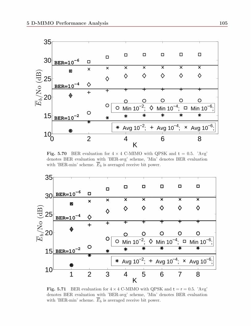
5.70 BER evaluation for 4 × 4 C-MIMO with QPSK and t = 0.5. ’Avg’ denotes BERevaluation with ’BER-avg’ scheme, ’Min’ denotes BER evaluation with ’BER-min’scheme. Eb is averaged receive bit power. . . . . . . . . . . . . . . . . . . . . . . . 105
5.71 BER evaluation for 4×4 C-MIMO with QPSK and t = r = 0.5. ’Avg’ denotes BERevaluation with ’BER-avg’ scheme, ’Min’ denotes BER evaluation with ’BER-min’scheme. Eb is averaged receive bit power. . . . . . . . . . . . . . . . . . . . . . . . 105
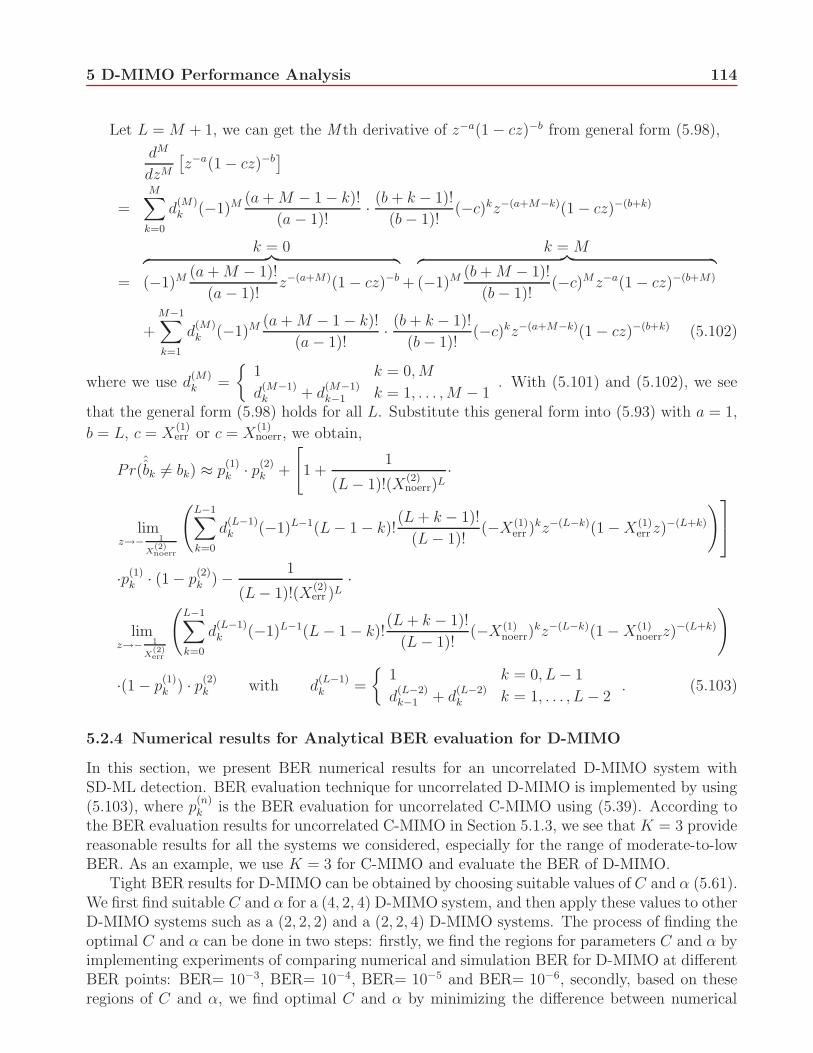
5.72 Numerical and simulation BER for uncorrelated (4,2,4) DMIMO d(1) = d(2) = 1kmwith SD-ML for QPSK and 16QAM. Parameter settings C and α are employedfrom Table 5.9, Eb is transmit bit power . . . . . . . . . . . . . . . . . . . . . . . 116
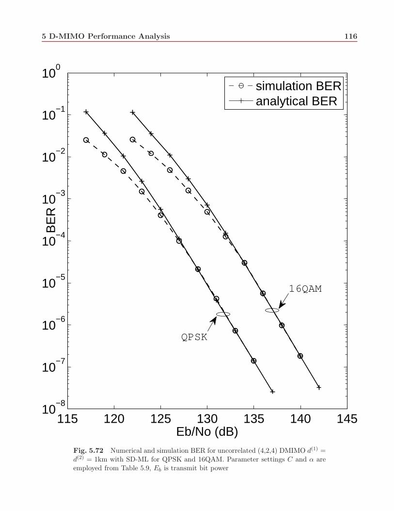
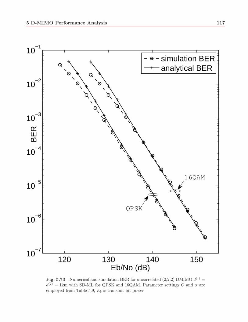
5.73 Numerical and simulation BER for uncorrelated (2,2,2) DMIMO d(1) = d(2) = 1kmwith SD-ML for QPSK and 16QAM. Parameter settings C and α are employedfrom Table 5.9, Eb is transmit bit power . . . . . . . . . . . . . . . . . . . . . . . 117
5.74 Numerical and simulation BER for uncorrelated (2,2,4) DMIMO d(1) = d(2) = 1kmwith SD-ML for QPSK and 16QAM. Parameter settings C and α are employedfrom Table 5.9, Eb is transmit bit power . . . . . . . . . . . . . . . . . . . . . . . 118
B.1 Structure of Dn2in one branch of constellation . . . . . . . . . . . . . . . . . . . . 121
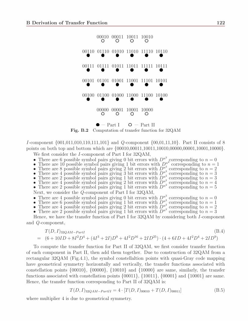
B.2 Computation of transfer function for 32QAM . . . . . . . . . . . . . . . . . . . . . 122
4.1 The performance gain of D-MIMO over C-MIMO for SD-ML with f = 1, g = 0 atBER= 10−5 . . . . . . . . . . . . . . . . . . . . . . . . . . . . . . . . . . . . . . . 20
4.2 The performance gain of D-MIMO over C-MIMO for MMSE-OSIC with f = 0, g =1 at BER= 10−5 . . . . . . . . . . . . . . . . . . . . . . . . . . . . . . . . . . . . . 20
5.1 Transfer function for QPSK, 16QAM, 32QAM and 64QAM . . . . . . . . . . . . . 595.2 Values of K required for tight BER approximation of uncorrelated C-MIMO . . . 615.3 Values of K required for tight BER approximation of C-MIMO when space cor-
relation at receiver only, r = 0.3 . . . . . . . . . . . . . . . . . . . . . . . . . . . . 765.4 Values of K required for tight BER approximation of C-MIMO when space cor-
relation at transmitter only with ’BER-avg’ technique, t = 0.3 . . . . . . . . . . . 765.5 Values of K required for tight BER approximation of C-MIMO when space cor-
relation at transmitter only with ’BER-min’ technique, t = 0.3 . . . . . . . . . . . 765.6 Values of K required for tight BER approximation of C-MIMO when space cor-
relation at receiver only, r = 0.5 . . . . . . . . . . . . . . . . . . . . . . . . . . . . 775.7 Values of K required for tight BER approximation of C-MIMO when space cor-
relation at transmitter only with ’BER-avg’ technique, t = 0.5 . . . . . . . . . . . 775.8 Values of K required for tight BER approximation of C-MIMO when space cor-
relation at transmitter only with ’BER-min’ technique, t = 0.5 . . . . . . . . . . . 775.9 C and α for D-MIMO with different modulation schemes . . . . . . . . . . . . . . 115
D.1 List of C software files for MMSE-OSIC detection scheme in enclosed CD . . . . . 128D.2 List of C software files for SD-ML detection scheme in enclosed CD . . . . . . . . 129D.3 Simulation parameters of the input file . . . . . . . . . . . . . . . . . . . . . . . . 130D.4 Parameters of the output file . . . . . . . . . . . . . . . . . . . . . . . . . . . . . . 130
xiii
List of Acronyms
16QAM 16-point Quadrature Amplitude Modulation32QAM 16-point Quadrature Amplitude Modulation64QAM 64-point Quadrature Amplitude ModulationAWGN Additive White Gaussian NoiseBER Bit Error RateC-MIMO Co-located MIMOCSI Channel State InformationD-MIMO Distributed MIMOLLR Logarithmic Likelihood RatioMIMO Multiple-Input Multiple-OutputML Maximum LikelihoodMMSE Minimum Mean Square ErrorMS Mobile StationOSIC Ordered Successive Interference CancelationPEP Pairwise Error ProbabilityQAM Quadrature Amplitude ModulationQPSK Quadrature Phase Shift KeyingSD Sphere DecodingSER Symbol Error RateSNR Signal to Noise RatioV-BLAST Vertical Bell Labs Layered Space-TimeVSER Vector Symbol Error RateZF Zero forcing
xiv
Notational Convention
(·)T Transpose of the argument(·)H Hermitian transpose of the argument(·)∗ Complex conjugate of the argument| · | Magnitude of scaler argument‖ · ‖2 Square norm of the vector argumentb Column vector bA Matrix Aai ith column vector of matrix A
A1/2 Square root of matrix AIN N -dimension identity MatrixA Set A|A| Cardinality of set A∅ Empty setdiag(·) Block diagonal matrixtr(A) Trace of matrix AN (µ, σ2) Normal distribution with mean µ and variance σ2
CN (µ, σ2) Complex Normal distribution with mean µ and variance σ2
EX [·] Expected value over random variable XEX|Y [·] Conditional expectation of X given event YfX(x) Probability density function (PDF) of random variable XfX|Y (x) Conditional probability density function (PDF) of random variable X
given random variable YFX(x) Cumulative distribution function (CDF) of random variable XFX|Y (x) Conditional cumulative distribution function (CDF) of random variable X
given random variable YPr[X] Probability of event XPr[X|Y ] Conditional probability of event X given event Y(
MN
)Binomial coefficient
ℜ(·) Real part of a complex numberℑ(·) Imaginary part of a complex number
Q(·) Q-function with Q(x) =1√2π
∫ ∞
x
e−u2
2 du
1
Chapter 1: Introduction
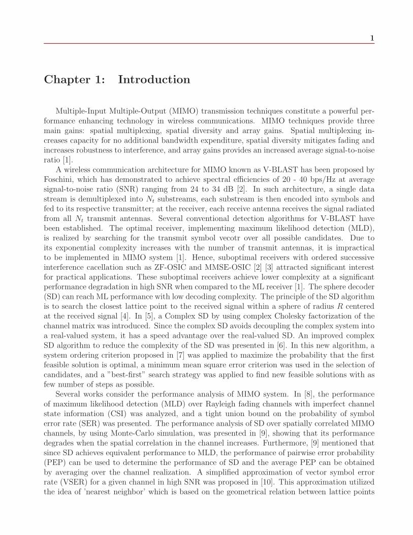
Multiple-Input Multiple-Output (MIMO) transmission techniques constitute a powerful per-formance enhancing technology in wireless communications. MIMO techniques provide threemain gains: spatial multiplexing, spatial diversity and array gains. Spatial multiplexing in-creases capacity for no additional bandwidth expenditure, spatial diversity mitigates fading andincreases robustness to interference, and array gains provides an increased average signal-to-noiseratio [1].
A wireless communication architecture for MIMO known as V-BLAST has been proposed byFoschini, which has demonstrated to achieve spectral efficiencies of 20 - 40 bps/Hz at averagesignal-to-noise ratio (SNR) ranging from 24 to 34 dB [2]. In such architecture, a single datastream is demultiplexed into Nt substreams, each substream is then encoded into symbols andfed to its respective transmitter; at the receiver, each receive antenna receives the signal radiatedfrom all Nt transmit antennas. Several conventional detection algorithms for V-BLAST havebeen established. The optimal receiver, implementing maximum likelihood detection (MLD),is realized by searching for the transmit symbol vecotr over all possible candidates. Due toits exponential complexity increases with the number of transmit antennas, it is impracticalto be implemented in MIMO system [1]. Hence, suboptimal receivers with ordered successiveinterference cacellation such as ZF-OSIC and MMSE-OSIC [2] [3] attracted significant interestfor practical applications. These suboptimal receivers achieve lower complexity at a significantperformance degradation in high SNR when compared to the ML receiver [1]. The sphere decoder(SD) can reach ML performance with low decoding complexity. The principle of the SD algorithmis to search the closest lattice point to the received signal within a sphere of radius R centeredat the received signal [4]. In [5], a Complex SD by using complex Cholesky factorization of thechannel matrix was introduced. Since the complex SD avoids decoupling the complex system intoa real-valued system, it has a speed advantage over the real-valued SD. An improved complexSD algorithm to reduce the complexity of the SD was presented in [6]. In this new algorithm, asystem ordering criterion proposed in [7] was applied to maximize the probability that the firstfeasible solution is optimal, a minimum mean square error criterion was used in the selection ofcandidates, and a ”best-first” search strategy was applied to find new feasible solutions with asfew number of steps as possible.
Several works consider the performance analysis of MIMO system. In [8], the performanceof maximum likelihood detection (MLD) over Rayleigh fading channels with imperfect channelstate information (CSI) was analyzed, and a tight union bound on the probability of symbolerror rate (SER) was presented. The performance analysis of SD over spatially correlated MIMOchannels, by using Monte-Carlo simulation, was presented in [9], showing that its performancedegrades when the spatial correlation in the channel increases. Furthermore, [9] mentioned thatsince SD achieves equivalent performance to MLD, the performance of pairwise error probability(PEP) can be used to determine the performance of SD and the average PEP can be obtainedby averaging over the channel realization. A simplified approximation of vector symbol errorrate (VSER) for a given channel in high SNR was proposed in [10]. This approximation utilizedthe idea of ’nearest neighbor’ which is based on the geometrical relation between lattice points
1 Introduction 2
and was varified by simulation over three kinds of channels: unitary channel, dense channel andsparse channel. Due to the difficulty of analyzing the performance of MIMO with optimal orderingsymbol-by-symbol detection algorithm, [11] provided the theoretical analysis on the performanceof VSER for ZF-SIC with fixed order over Rayleigh fading channel. A closed-form analyticalexpression for average BER of a 2 ×NR system when the optimal ordering is implemented wasderived in [12]. In [13], the BER performances of ZF-SIC and MMSE-SIC for the NT -th layerwithout optimal ordering have been analyzed. The SER performance of linear MMSE detectionfor a small number of transmit and receive antennas was analyzed in [14].
Due to the increased capacity needs, MIMO techniques are anticipated to be widely employedin future wireless networks. However in realistic systems, increasing the number of antennas ina restricted space reduces the inter-antenna spacing, leading to an increase in spatial correlationthat could limit the capacity gain of a traditional co-located MIMO (C-MIMO) [15]. Furthermore,C-MIMO when affected by shadowing can not improve link quality [15]. These reasons motivateus to investigate Distributed MIMO (D-MIMO) scheme, which can potentially remedy some ofthe problems associated with conventional C-MIMO systems. The main feature of D-MIMO isthat multiple antennas at one end of a communication link are distributed among multiple widely-separated radio Ports (i.e. base stations) [15]. In [15] [16] [17], a composite fading channel modelthat addresses the small-scale fast fading and large-scale fading for D-MIMO was presented. Itshows that the composite fading channel from MS to a radio Port is a product of a large-scalefading coefficient and a small-scale fading matrix.
Channel capacity for D-MIMO systems has attracted considerable research interest. In [16],the influence of macroscopic diversity on the capacity of D-MIMO with a composite channelmodel by using Monte-Carlo simulation has been presented and simulation results showed thatmultiple ports are essential to achieve high channel capacity both for the uplink and the downlink.Capacity loss due to spatial correlation and shadowing has been analyzed in [15] to demonstratethe advantage of D-MIMO versus C-MIMO. Mean spectral efficiency (MSE) and mean outagespectral efficiency (MOSE) metrics for D-MIMO and C-MIMO have been derived in [18] by apply-ing Gaussian approximation to the distribution of the mutual information (MI). Analytical andsimulation results show that due to macro-diversity gain, D-MIMO has significant larger MOSEthan C-MIMO. In [19], the authors proved that MI of D-MIMO is asymptotically equivalent toa Gaussian random variable and derive a closed-form approximation of the outage probabilityfor D-MIMO systems.
The BER performance of an uplink distributed-antenna/direct-sequence code-division multiple-access wireless communication system (DA/DS-CDMA) over composite lognormal shadowingslow-fading and Nakagami-m fast-fading channels is analyzed and evaluated in [20], where onlyone transmit antenna per user is considered and both correlation-based single-user detector(SUD) and MMSE-assisted multiuser detector (MUD) are employed. Simulation results for BERperformance of a downlink distributed antenna system (DAS) with only one receive antennaare presented in [21], where both SD and zero forcing (ZF) detection schemes are considered.However, to the author’s best knowledge, there is no research work which deals with the BERperformance analysis of a generalized D-MIMO system [15] [16] in literatures.
In this thesis, we propose a bit level combining scheme which combines the detected bitsfrom all Ports, aided by use of bit reliability information. By using such a bit combining schemeat the Fusion Center, bit detection for D-MIMO system is achieved with a complexity suitablefor practical applications. We derive the bit reliability information by applying logarithmic
1 Introduction 3
likelihood ratios (LLR) [22] [23] [24] and using the max-log approximation [25]. We present BERperformance for both C-MIMO and D-MIMO over a composite Rayleigh-lognormal channel byusing Monte-Carlo simulations for SD-ML and MMSE-OSIC detection. Furthermore, we providetheoretical BER performance analysis for C-MIMO and D-MIMO with SD-ML detection over acomposite Rayleigh-lognormal channel respectively, with consideration of spatial correlation andno spatial correlation.
The contributions of this thesis are:
• Proposed bit level combining scheme with bit reliability information at the Fusion Centerin D-MIMO and derived bit reliability information based on logarithmic likelihood ratio.
• Extended software development to D-MIMO with bit combining scheme and performedcomputer simulations to show BER performance of a 4×4 C-MIMO and BER performanceof a (4,2,4) D-MIMO over a composite Rayleigh-lognormal channel by considering MMSE-OSIC and SD-ML detection schemes for QPSK, 16QAM, 32QAM and 64QAM.
• Proposed theoretical BER evaluation scheme for C-MIMO with SD-ML detection over acomposite Rayleigh-lognormal channel with consideration of both spatial correlation andno spatial correlation.
• Proposed theoretical BER evaluation scheme for D-MIMO with SD-ML detection over acomposite Rayleigh-lognormal channel with consideration of both spatial correlation andno spatial correlation.
This thesis is organized as follows. Chapter 2 describes the system and channel model ofD-MIMO. In Chapter 3, the bit level combining scheme is presented and bit reliability informa-tion is derived. Furthermore, two detection schemes, MMSE-OSIC and SD-ML, are reviewed.Computer simulation results considering both perfect CSI and imperfect CSI as well as chan-nel spatial correlation are presented in chapter 4. In chapter 5, BER performance analysis forboth C-MIMO and D-MIMO over a composite fading channel with SD-ML detection as wellas corresponding numerical results are presented. Discussions and conclusions are presented inchapter 6. Appendix A illustrates partial fraction expension of a rational function. In AppendixB, we present the derivation of transfer function for square QAM constellaton and 32QAM. Theapplication of Residue theorem to evaluate integrals is illstrated in Appendix C. An overviewand user guide to the source code used to generate the simulations are included in Appendix D,and an attached CD contains all C source codes.
4
Chapter 2: System and Channel Model of D-MIMO
2.1 D-MIMO System Model
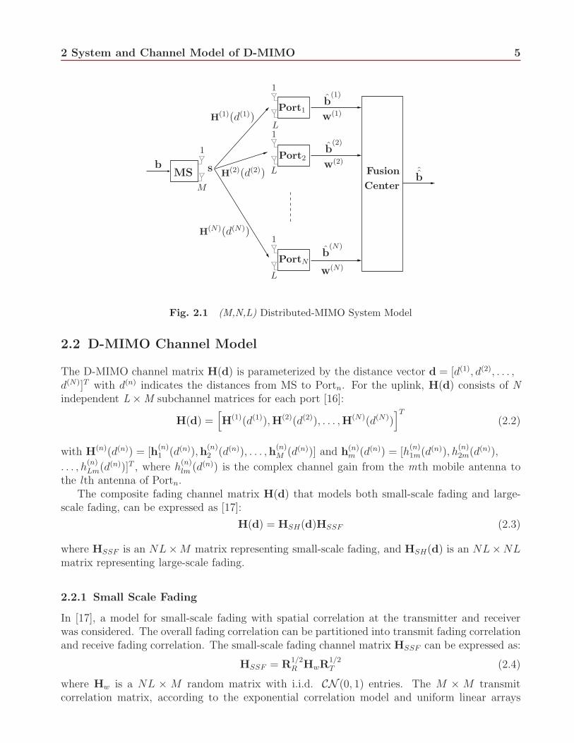
A D-MIMO system consisting of one transmit node, or Mobile Station (MS), and N geograph-ically dispersed receive nodes, or Base Stations (Ports) is illustrated in Fig. 2.1. The MStransmitter employs M co-located antennas, and each Port receiver has L co-located antennas(L ≥ M). Such system can be referred to as an (M,N,L) D-MIMO system [16]. Let Portn be thenth Port, and the channel from the MS to Portn be characterized by an L×M matrix H(n)(d(n))which is a product of a large-scale fading coefficient hsh,n(d
(n)) and a small-scale fading matrix
H(n)SSF , hence H(n)(d(n)) = hsh,n(d
(n)) · H(n)SSF , where d(n) is the distance between MS and Portn.
A single data stream, or transmitted bit vector b, has components bk ∈ {0, 1}, k = 1, . . . ,MQ0
where Q0 = log2Q and Q is the symbol constellation size. The data stream b is demultiplexedinto M substreams, each mapped into symbol si, i = 1, . . . ,M and fed to its respective transmitantenna [2], forming the transmitted symbol vector s of dimension M. The detected bit vector at
Portn is b(n)
, and is of dimension MQ0. Furthermore, w(n) is a bit-level reliability information
vector at Portn, of dimension MQ0. Each port passes b(n)
and w(n) to the Fusion Center (FC)
where the output bit vectorˆb of dimension MQ0 is produced based on a bit level combining
scheme we proposed in Chapter 3. We assume the FC is part of the core network, and hence thelinks from the ports are capacity limited. For example in LTE networks, the interface betweenthe base station and the core network is referred to as the S1 interface. It is usually carriedeither over a high-speed copper or fiber cable, or alternatively over a high-speed microwave link,which are, for example, based on Ethernet [26].
We assume that the wireless channel is static during a symbol duration, and experiencesflat-fading. Furthermore, we also assume perfect CSI is available at all radio port receivers. Theoverall uplink received signal can be written as [16] [18]:
r = H(d)s + n (2.1)
where r = [r1, . . . , rNL]T is the received signal vector at all ports, s = [s1, . . . , sM ]T is the trans-mitted symbol vector with unit transmit power satisfying E(sHs) = 1. Assuming the transmit
power is equally divided among transmit antennas, E(ssH) = σ2sIM =
1
MIM . Furthermore,
n = [n1, . . . , nNL]T is the complex additive white Gaussian noise vector with E[n] = 0 and co-variance matrix E[nnH ] = σ2
nINL. H(d) is an NL×M composite channel matrix with influenceof small-scale fading as well as large-scale fading and d is an N × 1 distance vector with the nthelement indicats the distance between MS and Portn.
2 System and Channel Model of D-MIMO 5
MSb s
1
1
1
1
L
L
L
M
H(1)(d(1))
H(2)(d(2))
H(N)(d(N))
Port1
Port2
PortN
b(1)
b(2)
b(N)
w(1)
w(2)
w(N)
ˆb
Fusion
Center
Fig. 2.1 (M,N,L) Distributed-MIMO System Model
2.2 D-MIMO Channel Model
The D-MIMO channel matrix H(d) is parameterized by the distance vector d = [d(1), d(2), . . . ,d(N)]T with d(n) indicates the distances from MS to Portn. For the uplink, H(d) consists of Nindependent L × M subchannel matrices for each port [16]:
H(d) =[
H(1)(d(1)),H(2)(d(2)), . . . ,H(N)(d(N))]T
(2.2)
with H(n)(d(n)) = [h(n)1 (d(n)),h
(n)2 (d(n)), . . . ,h
(n)M (d(n))] and h(n)
m (d(n)) = [h(n)1m(d(n)), h
(n)2m(d(n)),
. . . , h(n)Lm(d(n))]T , where h
(n)lm (d(n)) is the complex channel gain from the mth mobile antenna to
the lth antenna of Portn.The composite fading channel matrix H(d) that models both small-scale fading and large-
scale fading, can be expressed as [17]:
H(d) = HSH(d)HSSF (2.3)
where HSSF is an NL×M matrix representing small-scale fading, and HSH(d) is an NL×NLmatrix representing large-scale fading.
2.2.1 Small Scale Fading
In [17], a model for small-scale fading with spatial correlation at the transmitter and receiverwas considered. The overall fading correlation can be partitioned into transmit fading correlationand receive fading correlation. The small-scale fading channel matrix HSSF can be expressed as:
HSSF = R1/2R HwR
1/2T (2.4)
where Hw is a NL × M random matrix with i.i.d. CN (0, 1) entries. The M × M transmitcorrelation matrix, according to the exponential correlation model and uniform linear arrays
2 System and Channel Model of D-MIMO 6
employed at MS, is given by [27]:
RT =
1 t∗ . . . (t(M−1)2)∗
t 1 . . . (t(M−2)2)∗
......
. . ....
t(M−1)2
t(M−2)2 . . . 1
(2.5)
where t ∈ [0, 1] is fading correlation coefficient of neighboring transmit antennas, and (·)∗ denotescomplex conjugation. Since RT is Hermitian, it is diagonalizable by a unitary matrix U: RT =UDU−1 where D is a diagonal matrix consisting of the eigenvalues of RT , and hence:
R1/2T = UD1/2U−1 (2.6)
Same definition of matrix square root applies to receive correlation matrix RR.For D-MIMO receiver, we assume independent small-scale fading at different ports due to
large spacing between them, with small-scale fading within each port being correlated due toinsufficient spacing between antennas in a port. According to this assumption, the NL × NLreceive correlation matrix RR can be expressed as:
RR = diag(R(1)R ,R
(2)R , . . . ,R
(N)R ) (2.7)
where diag(·) denotes a block diagonal matrix, having main diagonal blocks square matrices,
R(1)R ,R
(2)R , . . . ,R
(N)R . The receive correlation matrix at Portn, R
(n)R , also follows the exponential
correlation model,
R(n)R =
1 (rn)∗ . . . (r(L−1)2
n )∗
rn 1 . . . (r(L−2)2
n )∗
......
. . ....
r(L−1)2
n r(L−2)2
n . . . 1
(2.8)
where rn is the fading correlation coefficient of neighboring receive antennas at Portn.From (2.4), (2.7), we get the equivalent small-scale fading matrix:
HSSF =
(R(1)R )1/2
(R(2)R )1/2
. . .
(R(N)R )1/2
H(1)w
H(2)w...
H(N)w
· (RT )1/2
=
(R(1)R )1/2H(1)
w (RT )1/2
(R(2)R )1/2H(2)
w (RT )1/2
...
(R(N)R )1/2H(N)
w (RT )1/2
(2.9)
where R(n)R is an L × L receive correlation matrix of Portn, H(n)
w is an L × M matrix with
i.i.d. CN (0, 1) entries, RT is an M × M transmit correlation matrix of MS and H(n)SSF =
(R(n)R )1/2H(n)
w (RT )1/2 is an L×M subchannel small scale fading matrix between MS and Portn,n = 1, 2, . . . , N .
2 System and Channel Model of D-MIMO 7
2.2.2 Large Scale Fading
Large-scale fading is the effect of combined path loss and shadowing. Due to large spacingbetween Ports, we assume that shadow fading between the N base station ports and the MS areindependent, and antennas at the same port are experiencing same shadowing effect [15] [16].
Models for combined path loss and shadowing can be represented as a power decrease versusdistance along with the random attenuation due to shadowing. From [28], [29] the received signal
power at the nth base station P(n)R is given in terms of the transmitted signal power PT by:
P(n)R =
A
(d(n)
d0)τ
· φn · PT (2.10)
where A is the path gain at reference distance d0, d(n) is the distance between MS and Portn,
τ is the path-loss exponent that strongly depends on the base station antenna height and theterrain category [28] with typical values 3.7 − 6.5 in Urban macrocells [29]. Furthermore, φn isa log-normal shadow fading variable of Portn, with 10 log10 φn ∼ N (0, σ2
φdB). Empirical studies
support σφdBranging from 4dB to 13dB [29] for outdoor channels.
At 1.9GHz, A is close to the free-space path gain at d0 = 100m [28], and from [29]:
A =
(λ
4πd0
)2
(2.11)
where λ =c
fcis the wavelength in meters, c is the speed of light and fc is the carrier frequency.
Combining (2.10)-(2.11), we have:
P(n)R =
(c
fc·4·π·d0
)2
(d(n)
d0
)τ · φn · PT =
(c
fc · 4 · π
)2
· d(τ−2)0 · φn
[d(n)]τ· PT (2.12)
Define κ =
(c
fc · 4 · π
)2
· d(τ−2)0 , we have:
hsh,n(d(n)) =
√
κ · φn
[d(n)]τ(2.13)
where hsh,n(d(n)) represents the channel coefficient affected by shadowing and path loss. This
model applies to base station antenna heights from 10 to 80m, BS-to-MS distances from 0.1 to8 km [28]. Finally the channel matrix of large-scale fading is:
HSH = diag[hsh,1(d(1)) · IL, hsh,2(d
(2)) · IL, · · · , hsh,N(d(N)) · IL] (2.14)
where IL is an L-dimension identity matrix.From (2.2), (2.3), (2.9), (2.14), we can get the composite fading channel matrix H(d) as:
H(d) =[
H(1)(d(1)),H(2)(d(2)), . . . ,H(N)(d(N))]T
(2.15)
where
H(n)(d(n)) = hsh,n(d(n))[(R
(n)R )1/2H(n)
w (RT )1/2] = hsh,n(d(n))H
(n)SSF (2.16)
is the L × M subchannel matrix associated with the link from MS to Portn, n = 1, 2, . . . , N .
8
Chapter 3: Combining with Reliability Information
After receiving the detected bits from all Ports, the Fusion Center makes the final bit detectionby using bit combining aided with bit reliability information. In this chapter, we present analgorithm for bit combing and derive the bit reliability information. Furthermore, two MIMOdetection schemes, MMSE-OSIC and SD-ML are reviewed in this chapter.
3.1 Bit by Bit Combing at the Fusion Center
Let b(n)k be the kth detected bit at Portn, k = 1, . . . ,MQ0. Let p
(n)k be the probability that b
(n)k
is in error, assume p(n)k ≤ 1
2. Let b ∈ {0, 1}, bk ∈ {0, 1} be the kth transmitted bit. Define
dH(b(n)k , b) =
{
1 b(n)k 6= b
0 b(n)k = b
as the Hamming distance between b(n)k and b. Then:
P[
b(1)k , . . . , b
(N)k |bk = b
]
=N∏
n=1
P[
b(n)k |bk = b
]
=
N∏
n=1
[
p(n)k
]dH(b(n)k ,b)
·[
1 − p(n)k
]1−dH (b(n)k ,b)
=
N∏
n=1
[
1 − p(n)k
]
·N∏
n=1
[
p(n)k
1 − p(n)k
]dH(b(n)k ,b)
(3.1)
where the first equality is because b(1)k , . . . , b
(N)k are independent, the second equality is based on:
P[
b(n)k |bk = b
]
=
{
p(n)k b
(n)k 6= b
1 − p(n)k b
(n)k = b
=[
p(n)k
]dH(b(n)k ,b)
·[
1 − p(n)k
]1−dH(b(n)k ,b)
(3.2)
Taking the logarithm of (3.1), we have:
logP[
b(1)k , . . . , b
(N)k |bk = b
]
=N∑
n=1
log[
1 − p(n)k
]
−D[
{b(1)k , . . . , b(N)k }, b
]
(3.3)where
D[
{b(1)k , . . . , b(N)k }, b
]
=N∑
n=1
dH(b(n)k , b) · log
[
1 − p(n)k
p(n)k
]
. (3.4)
Since p(n)k ≤ 1
2, we have D
[
{b(1)k , . . . , b(N)k }, b
]
≥ 0.
After receiving the detected bits from all of the N ports, the Fusion Center will make the final
bit detectionˆbk corresponding to each transmitted bit bk by implementing the Maximum Likeli-
hood decision rule,ˆbk = arg max
b∈{0,1}P[
b(1)k , . . . , b
(N)k |bk = b
]
= arg minb∈{0,1}
D[
{b(1)k , . . . , b(N)k }, b
]
.
When there is a tie, thenˆbk = 1 with probability 1/2 and
ˆbk = 0 with probability 1/2. With
equal a-prior probabilities for bk, this will result in minimizing the probability of error.
Define ∆[
b(1)k , . . . , b
(N)k
]
= D[
{b(1)k , . . . , b(N)k }, 1
]
− D[
{b(1)k , . . . , b(N)k }, 0
]
. The decision rule
3 Combining with Reliability Information 9
will be: ∆[
b(1)k , . . . , b
(N)k
]
< 0,ˆbk = 1
> 0,ˆbk = 0
= 0,ˆbk = 1 with probability 1/2 andˆbk = 0 with probability 1/2
. From (3.4), we have:
∆[
b(1)k , . . . , b
(N)k
]
=
N∑
n=1
[
dH(b(n)k , 1) − dH(b
(n)k , 0)
]
log
[
1 − p(n)k
p(n)k
]
=
N∑
n=1
(−1)b(n)k log
[
1 − p(n)k
p(n)k
]
(3.5)Since p
(n)k are not available, (3.5) can not be used as is. Recognizing that log
[
1−p(n)k
p(n)k
]
can be
considered as reliability indication, we suggest the following class of decision rules:
∆[
b(1)k , . . . , b
(N)k
]
< 0,ˆbk = 1
> 0,ˆbk = 0
= 0,ˆbk = 1 with probability 1/2 andˆbk = 0 with probability 1/2
(3.6)
where∆[
b(1)k , . . . , b
(N)k
]
=
N∑
n=1
(−1)b(n)k w
(n)k (3.7)
and w(n)k are reliability informations with w
(n)k ≥ 0. The larger is w
(n)k the more reliable is b
(n)k .
3.2 Bit Reliability Information
Bit reliability information, depends on the type of MIMO detection employed at the Ports. Inthis work, we consider MMSE-OSIC as well as Sphere Decoding.
3.2.1 MMSE-OSIC Detection Scheme in MIMO
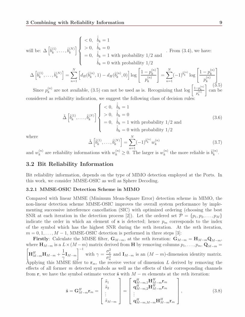
Compared with linear MMSE (Minimum Mean-Square Error) detection scheme in MIMO, thenon-linear detection scheme MMSE-OSIC improves the overall system performance by imple-menting successive interference cancellation (SIC) with optimized ordering (choosing the bestSNR at each iteration in the detection process [2]). Let the ordered set P = {p1, p2, . . . , pM}indicate the order in which an element of s is detected; hence pm corresponds to the indexof the symbol which has the highest SNR during the mth iteration. At the mth iteration,m = 0, 1, . . . ,M − 1, MMSE-OSIC detection is performed in three steps [3]:
Firstly: Calculate the MMSE filter, GM−m, at the mth iteration: GM−m = HM−mQM−m,where HM−m is a L×(M−m) matrix derived from H by removing columns p1, . . . , pm, QM−m =[
HHM−mHM−m +
1
γIM−m
]−1
with γ =σ2
s
σ2n
and IM−m is an (M −m)-dimension identity matrix.
Applying this MMSE filter to rm, the receive vector of dimension L derived by removing theeffects of all former m detected symbols as well as the effects of their corresponding channelsfrom r, we have the symbol estimate vector s with M −m elements at the mth iteration:
s = GHM−mrm =
s1
s2...sM−m
=
qHM−m,1H
HM−mrm
qHM−m,2H
HM−mrm
...qH
M−m,M−mHHM−mrm
, (3.8)
3 Combining with Reliability Information 10
where si is the ith element of s and qM−m,j is the j th column vector of QM−m. During theinitialization stage (m = 0), we have HM = H and r0 = r.
Secondly: The element of s with the highest SNR is detected. In [3], this element isassociated with the smallest diagonal entry of QM−m: pm+1 = arg min
iqM−m,ii, where qM−m,ii are
the diagonal elements of matrix QM−m. We have the detected symbol:
spm+1 = Q[spm+1 ] = Q[qHM−m,pm+1
HHM−mrm] (3.9)
where Q[·] indicates the quantization procedure according to the signal constellation.Thirdly: We cancel the detected symbol spm+1 as well as its corresponding channel from the
receive vector rm, resulting in a new received vector for symbol detection of next (m+1 )th layer:
rm+1 = rm − spm+1hpm+1 (3.10)
Steps 1-3 are then performed for the (m+1 )th iteration with modified HM−(m+1), QM−(m+1)
and rm+1, till all the symbols sp1 , . . . , spMare detected.
The algorithm for V-BLAST with MMSE-OSIC [3] can be presented as:
Step 2. Determine HM−m by removing the pmth column from HM−m+1
Step 3. QM−m = [HHM−mHM−m + αIM−m]−1
Step 4. pm+1 = arg miniqM−m,ii
Step 5. spm+1 = qHM−m,pm+1
HHM−mrm
Step 6. spm+1 = Q[spm+1]
where α =σ2
n
σ2s
=1
γ. At Step 6. of each iteration, we consider spm+1 as the symbol estimate
corresponding to the pm+1th layer.
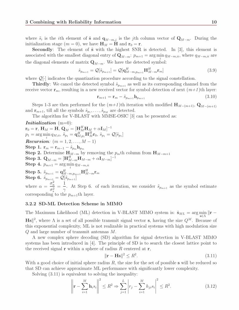
3.2.2 SD-ML Detection Scheme in MIMO
The Maximum Likelihood (ML) detection in V-BLAST MIMO system is: sML = arg mins∈Λ
‖r −Hs‖2, where Λ is a set of all possible transmit signal vector s, having the size QM . Because ofthis exponential complexity, ML is not realizable in practical systems with high modulation sizeQ and large number of transmit antennas M .
A new complex sphere decoding (SD) algorithm for signal detection in V-BLAST MIMOsystems has been introduced in [4]. The principle of SD is to search the closest lattice point tothe received signal r within a sphere of radius R centered at r,
‖r− Hs‖2 ≤ R2. (3.11)
With a good choice of initial sphere radius R, the size for the set of possible s will be reduced sothat SD can achieve approximate ML performance with significantly lower complexity.
Solving (3.11) is equivalent to solving the inequality:∥∥∥∥∥r −
M∑
i=1
hisi
∥∥∥∥∥
2
≤ R2 ⇒L∑
j=1
∣∣∣∣∣rj −
M∑
i=1
hjisi
∣∣∣∣∣
2
≤ R2. (3.12)
3 Combining with Reliability Information 11
Due to the general structure of H, (3.12) is an inequality with summation of L terms, and eachterm consists of M unknown parameters si, it is shown to be a nondeterministic polynomial-time(NP)-hard problem [4]. According to [5], ‖r − Hs‖2 can be decomposed as:
‖r −Hs‖2 = (s− s)HHHH(s− s) + rH(I − H(HHH)−1HH
)r (3.13)
where s is the unconstrained ML estimate of s: s = (HHH)−1HHr. Therefore, the SD detectionis equivalent to:
(s − s)HHHH(s− s) ≤ R2 (3.14)
Since Gramian matrix HHH is Hermitian and positive-definite, and applying Cholesky factor-ization, we have HHH = UHU, where U is an upper triangular M ×M matrix with positivediagonal entries. (Compared with QR factorization which needs M3 flops, Cholesky factorizationneeds only M3/3 flops [30]). Hence (3.14) can be written as:
(s − s)HUHU(s − s) = ‖U(s − s)‖2 =
∥∥∥∥∥∥∥∥∥
u11 u12 · · · u1M
0 u22 · · · u2M...
.... . .
...0 0 · · · uMM
s1 − s1
s2 − s2...
sM − sM
∥∥∥∥∥∥∥∥∥
2
≤ R2 (3.15)
Using the property of upper triangular matrix U, (3.15) implies the set of conditions:
M∑
k=m
∣∣∣∣∣
M∑
j=k
ukj(sj − sj)
∣∣∣∣∣
2
≤ R2 m = 1, . . . ,M (3.16)
Consider above conditions in the order from M to 1, we successively obtain the set of candidatesfor sm, symbol of mth layer, with back-substitution of given symbols sM , . . . , sm+1. Followingsare the detail processes:
Starting from layer m = M and only considering the bottom term of the Euclidean norm
in (3.15), the corresponding condition in (3.16) is: |sM − sM |2 6R2
u2MM
. A complex disk for
the M th layer DiskM is formed, with center sM = sM and radius RM = R2
u2MM
. Let A be the
set of whole constellation points. By searching the constellation points within the DiskM , wehave the set of candidates for sM : SM,cand = {a : a ∈ A and a within DiskM} and let thecandidate which is closest to the center sM be the temporary symbol detection of the M th layer:sM = arg min
a′∈SM,cand
|a′ − sM |2.Go to the upper layer m = M − 1 and consider the bottom two terms of the Euclidean norm
in (3.15), the implied condition in (3.16) will be:
With back-substitution of sM , we have DiskM−1, a complex disk for the (M-1 )th layer, with cen-
3 Combining with Reliability Information 12
ter sM−1 = sM−1−uM−1,M
uM−1,M−1(sM−sM) and radius RM−1 =
1
u2M−1,M−1
[R2−u2M,M |sM−sM |2]. Sim-
ilarly, we get the set of the candidates for sM−1: SM−1,cand = {a : a ∈ A and a within DiskM−1}and the temporary symbol detection of the (M-1 )th layer: sM−1 = arg min
a′∈SM−1,cand
|a′ − sM−1|2.In general, at layer m = i, considering the bottom M − i+ 1 terms of the Euclidean norm in
(3.15), the corresponding condition in (3.16) becomes:
with back-substitution of previously determined sj , j = M,M − 1, . . . , i + 1, a complex diskDiski of radius Ri (3.20) centered at si (3.19) is specified. The set of candidates for si isSi,cand = {a : a ∈ A and a within Diski} and the temporary symbol detection of ith layer issi = arg min
a′∈Si,cand
|a′ − si|2.The process is continued to (i−1)th layer and so on. At last, two possible things will happen:
1. The leaf node is reached (s1 is found), a feasible solution s is obtained. The new radius iscalculated: Rnew = ‖U(s − s)‖2, satisfying Rnew ≤ R2. Then re-do the search for betters with Rnew. In [6], a new algorithm of ’best-first’ search strategy was proposed to reduceSD complexity. In this new algorithm, the search resumes with the path that is closest tocompletion rather than restarting the search from the root node.
2. There is no leaf node reached at all, which means the initial radius R is too small so thatno feasible s can be found within the hypersphere. In such case, the initial radius R shouldbe increased and the search should be restart from root node again.
The center of a complex disk at ith layer, si of (3.19), is the symbol estimate of ith layer.Such SD-ML detection process can be performed by using a tree structure with M layers
as illustrated in Fig. 3.1. SD-ML starts searching from root of the tree and works down alongthe branch till the leaf node is reached. The nodes on the ith layer stands for Si,cand, the setof the candidates for si, which can be obtained from the bound (3.18) with back-substitution ofpreviously detected symbols. The nodes on the branch from the root to leaf with the smallestradius are chosen to be the symbol vector solution s.
3 Combining with Reliability Information 13
root node
leaf nodeM=4
(first layer)m = M − 3
m = M − 2
m = M − 1
m = M
Fig. 3.1 Tree Structure for Sphere Decoding with detection layer M = 4
The algorithm of SD [6] consists of the following steps with index i from 0 to M − 1:Step 1. Set the initial radius R, set flag = 0, compute unconstrained ML estimate s.Step 2. Initialize i = M , D = 0 and the candidate sets Sk,cand = ∅, k=0,. . . ,M-1. Set symboldetection vector s = 0 and symbol estimate vector s = 0. If flag = 1, set R = 1.2R.Step 3. Set i = i − 1, compute the symbol estimate si using (3.19) and obtain the candidateset for si within the range defined by (3.18).Step 4. If candidates for symbol si are found, goto step 7. Otherwise, goto step 5.Step 5. If the candidate sets for all symbols are nonempty Sk,cand 6= ∅, k = 0, . . . ,M − 1, gotostep 12. Otherwise, goto step 6.Step 6. If no solution has been found yet, set flag = 1 and goto step 2. Otherwise, output the”current-best” solution.Step 7. For each candidate of si found in Step 3, compute the corresponding distances δ =|(candidate of si)− si|2. Denote the smallest δ as δi, arrange these δ in increasing order and storethem in candidate set Si,cand (excluding δi). Set si equal to the candidate associated with δi.Step 8. Set D = D + u2
iiδi. If D < R, goto step 10. Otherwise, goto step 9.Step 9. If the candidate sets for all symbols are nonempty Sk,cand 6= ∅, k = 0, . . . ,M − 1, gotostep 12. Otherwise, goto step 6.Step 10. If i > 0, goto Step 3.Step 11. If i = 0, update the ’current-best’ solution with s, update the ’current-best’ symbolestimate with s and let R = D. If the candidate sets for all symbols are nonempty Sk,cand 6= ∅,k = 0, . . . ,M − 1, goto step 12. Otherwise, output the ”current-best” solution.Step 12. Select the nonempty candidate set closest to the last tree level and set i equal tothis level. Select the candidate with the smallest distance δ in set Si,cand, set δi equal to δcorresponding to this candidate and update si equal to this candidate, remove the first elementin set Si,cand and goto Step 8.
Compared with ML detector, which needs to perform exhaust search among all possibletransmitted symbol vector of size QM , the SD algorithm achieves approximate ML performancewith much lower complexity by only searching the points that lie within a hypersphere of radiusR around r. With a good choise of R, the roughly complexity of the algorithm is O(M3) [5].
3 Combining with Reliability Information 14
3.2.3 Bit Level Reliability Information
Consider a signal space constellation composed of the set of signal points A = {a1, . . . , aQ} anda mapping of Q0 information bits b1, . . . , bQ0 into the constellation points A where Q0 = log2Q.
Here, we consider quadrature amplitude modulation (QAM) with Gray mapping. Define A(0)i as
the set of constellation points for which bi = 0. Similarly, define A(1)i as the set of constellation
points for which bi = 1. Then for i = 1, 2, . . . , Q0, we have: A(0)i
⋂A(1)i = ∅ and A(0)
i
⋃A(1)i = A,
with |A(0)i | = |A(1)
i | = Q/2, where | · | denotes the cardinality of the set.Let bk be the kth transmitted bit and s be the symbol estimate. The a posteriori probability
ratio for the kth bit is: Λk =Pr{bk = 1|s}Pr{bk = 0|s} . According to Bayes Rule:
Pr{bk|s}Pr{s}Pr{bk}
=
Pr{s|bk}. With equally likely bk, we have: Λk =Pr{s|bk = 1}Pr{s|bk = 0} .
The reliability metrics (soft output) for bk are calculated in the form of logarithmic likelihoodratios (LLR) [22] [23]:
Lk = log Λk = logPr{s|bk = 1}Pr{s|bk = 0} = log
∑
a∈A(1)kPr{s|sk = a}
∑
a∈A(0)kPr{s|sk = a} . (3.21)
For an AWGN channel, (3.21) will be: Lk = log
∑
a∈A(1)k
exp(−γ|s− a|2)∑
a∈A(0)k
exp(−γ|s− a|2) [23][24], where γ is
the average SNR per symbol.
Applying the so-called max-log approximation [25]: log∑
j
exp(αj) ≈ maxj
(αj), the logarith-
mic likelihood ratio can be simplified as [23][24]:
Lk = γ
[
mina∈A
(0)k
{|s− a|2} − mina∈A
(1)k
{|s− a|2}]
(3.22)
In an M × L V-BLAST MIMO system, the symbol covariance matrix at the receiver can be
calculated as: E[(Hs)(Hs)H
]=
M∑
i=1
hihHi · σ2
si, since E(sis
∗j) =
{σ2
sii = j
0 i 6= j. Let ‖hi‖2 · σ2
si
be the receive power of symbol si. Since the transmit power is equally divided among transmit
antennas σsi=PT
Mand the AWGN noise on each channel has the same power σ2
n, the average
receive SNR for symbol si will be:γi ∝ ‖hi‖2 (3.23)
and it is the same for all bits associated with the same symbol.Due to the positive requirement of the reliability information, based on (3.22), we could
take
∣∣∣∣∣min
a∈A(0)k
{|s− a|2} − mina∈A
(1)k
{|s− a|2}∣∣∣∣∣
as the reliability weight for the kth bit. Let ak,j =
where lk,j = |s− ak,j| indicating the distance between s and ak,j. The larger the value of (3.24),the more reliable the detection of the kth bit is.
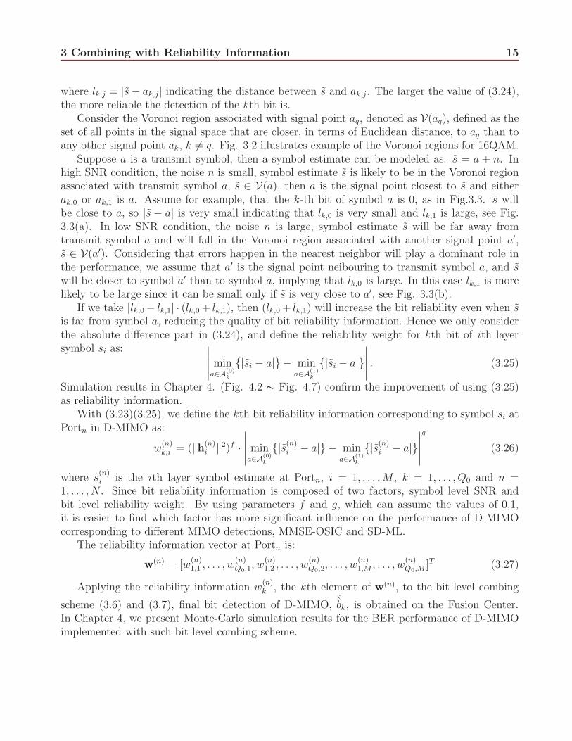
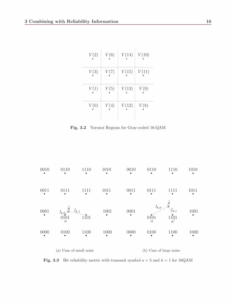
Consider the Voronoi region associated with signal point aq, denoted as V(aq), defined as theset of all points in the signal space that are closer, in terms of Euclidean distance, to aq than toany other signal point ak, k 6= q. Fig. 3.2 illustrates example of the Voronoi regions for 16QAM.
Suppose a is a transmit symbol, then a symbol estimate can be modeled as: s = a + n. Inhigh SNR condition, the noise n is small, symbol estimate s is likely to be in the Voronoi regionassociated with transmit symbol a, s ∈ V(a), then a is the signal point closest to s and eitherak,0 or ak,1 is a. Assume for example, that the k -th bit of symbol a is 0, as in Fig.3.3. s willbe close to a, so |s− a| is very small indicating that lk,0 is very small and lk,1 is large, see Fig.3.3(a). In low SNR condition, the noise n is large, symbol estimate s will be far away fromtransmit symbol a and will fall in the Voronoi region associated with another signal point a′,s ∈ V(a′). Considering that errors happen in the nearest neighbor will play a dominant role inthe performance, we assume that a′ is the signal point neibouring to transmit symbol a, and swill be closer to symbol a′ than to symbol a, implying that lk,0 is large. In this case lk,1 is morelikely to be large since it can be small only if s is very close to a′, see Fig. 3.3(b).
If we take |lk,0 − lk,1| · (lk,0 + lk,1), then (lk,0 + lk,1) will increase the bit reliability even when sis far from symbol a, reducing the quality of bit reliability information. Hence we only considerthe absolute difference part in (3.24), and define the reliability weight for kth bit of ith layersymbol si as: ∣
∣∣∣∣min
a∈A(0)k
{|si − a|} − mina∈A
(1)k
{|si − a|}∣∣∣∣∣. (3.25)
Simulation results in Chapter 4. (Fig. 4.2 ∼ Fig. 4.7) confirm the improvement of using (3.25)as reliability information.
With (3.23)(3.25), we define the kth bit reliability information corresponding to symbol si atPortn in D-MIMO as:
w(n)k,i = (‖h(n)
i ‖2)f ·∣∣∣∣∣min
a∈A(0)k
{|s(n)i − a|} − min
a∈A(1)k
{|s(n)i − a|}
∣∣∣∣∣
g
(3.26)
where s(n)i is the ith layer symbol estimate at Portn, i = 1, . . . ,M , k = 1, . . . , Q0 and n =
1, . . . , N . Since bit reliability information is composed of two factors, symbol level SNR andbit level reliability weight. By using parameters f and g, which can assume the values of 0,1,it is easier to find which factor has more significant influence on the performance of D-MIMOcorresponding to different MIMO detections, MMSE-OSIC and SD-ML.
The reliability information vector at Portn is:
w(n) = [w(n)1,1 , . . . , w
(n)Q0,1, w
(n)1,2 , . . . , w
(n)Q0,2, . . . , w
(n)1,M , . . . , w
(n)Q0,M ]T (3.27)
Applying the reliability information w(n)k , the kth element of w(n), to the bit level combing
scheme (3.6) and (3.7), final bit detection of D-MIMO,ˆbk, is obtained on the Fusion Center.
In Chapter 4, we present Monte-Carlo simulation results for the BER performance of D-MIMOimplemented with such bit level combing scheme.
3 Combining with Reliability Information 16
V (0)
V (1)
V (2)
V (3)
V (4)
V (5)
V (6)
V (7)
V (8)
V (9)
V (10)
V (11)
V (12)
V (13)
V (14)
V (15)
Fig. 3.2 Voronoi Regions for Gray-coded 16-QAM
0000
0001
0010
0011
0100
0101
0110
0111
1000
1001
1010
1011
1100
1101
1110
1111
s
a
lk,0lk,1
(a) Case of small noise
0000
0001
0010
0011
0100
0101
0110
0111
1000
1001
1010
1011
1100
1101
1110
1111
s
a a′
lk,0lk,1
(b) Case of large noise
Fig. 3.3 Bit reliability metric with transmit symbol a = 5 and k = 1 for 16QAM
17
Chapter 4: Computer Simulation Results
We present computer simulation results for bit error rate (BER) performance of a (4,2,4)
D-MIMO system and a 4×4 C-MIMO system. BER is defined as: BER=1
MQ0.
MQ0∑
k=1
Pr(ˆbk 6= bk)
and it is plotted versusEb
No=
σ2s
Q0σ2n
where Eb is transmit bit power. Monte-Carlo simulations
are used to obtain Pr(ˆbk 6= bk).
Two detection schemes are considered: MMSE-OSIC [3] and SD-ML [5] [6]. The consideredmodulation schemes include QPSK, 16QAM and 64QAM, all with Gray code mapping havingthe property that two adjacent symbols differ in only one single bit [29] [31]. We consider also32QAM with quasi-Gray code mapping where some symbols adjacent may not differ only in onebit. The construction of 32QAM is done by first forming a 4×8 rectangular 32QAM constellationwith Gray mapping. Then the last columns of symbols on the far left and far right are movedto the top and bottom [32]. This construction is shown in Fig 4.1 where arrows indicate movingdirections.
For each channel use, a new transmitted symbol vector of dimension M is randomly generatedand each symbol consists of Q0 binary bits. The composite fading channel (2.15) varies randomlyand independently from one use to another. The small scale fading channel matrix (2.9) isconsidered. In case of no space correlation at the transmitter and the reciever, each element ofthe small scale fading channel matrix is generated as i.i.d complex Gaussian random variablewith zero mean and unit variance. The large scale fading channel coefficient (2.13) is a functionof d(n) with parameters: fc = 1.9GHz, d0 = 100m, τ = 4 and σφdB
= 4. In addition, at eachSNR, the performance is averaged over at least 1 million channel realizations and a minimumof 500 frame errors are accumulated. A frame error is defined as the event ˆs 6= s where ˆs is thedetected symbol vector at the Fusion Center.
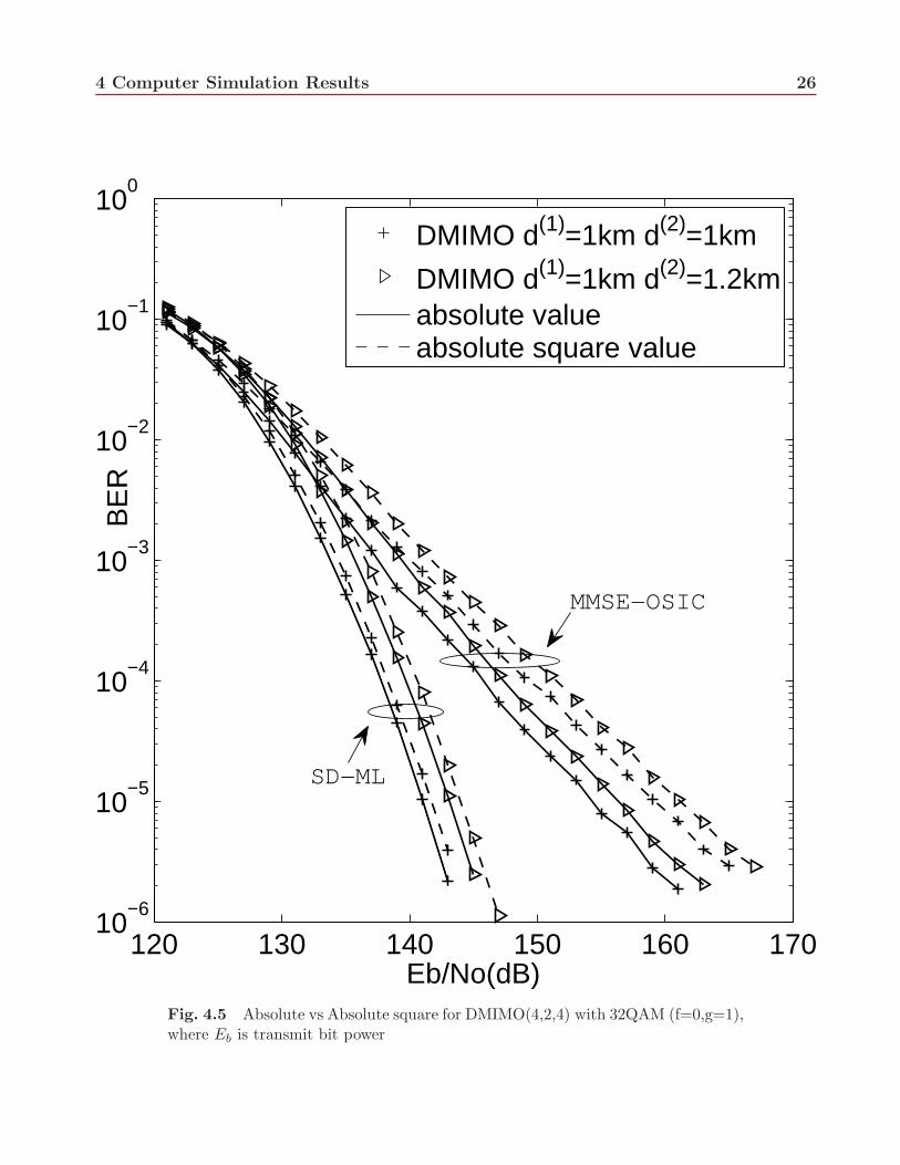
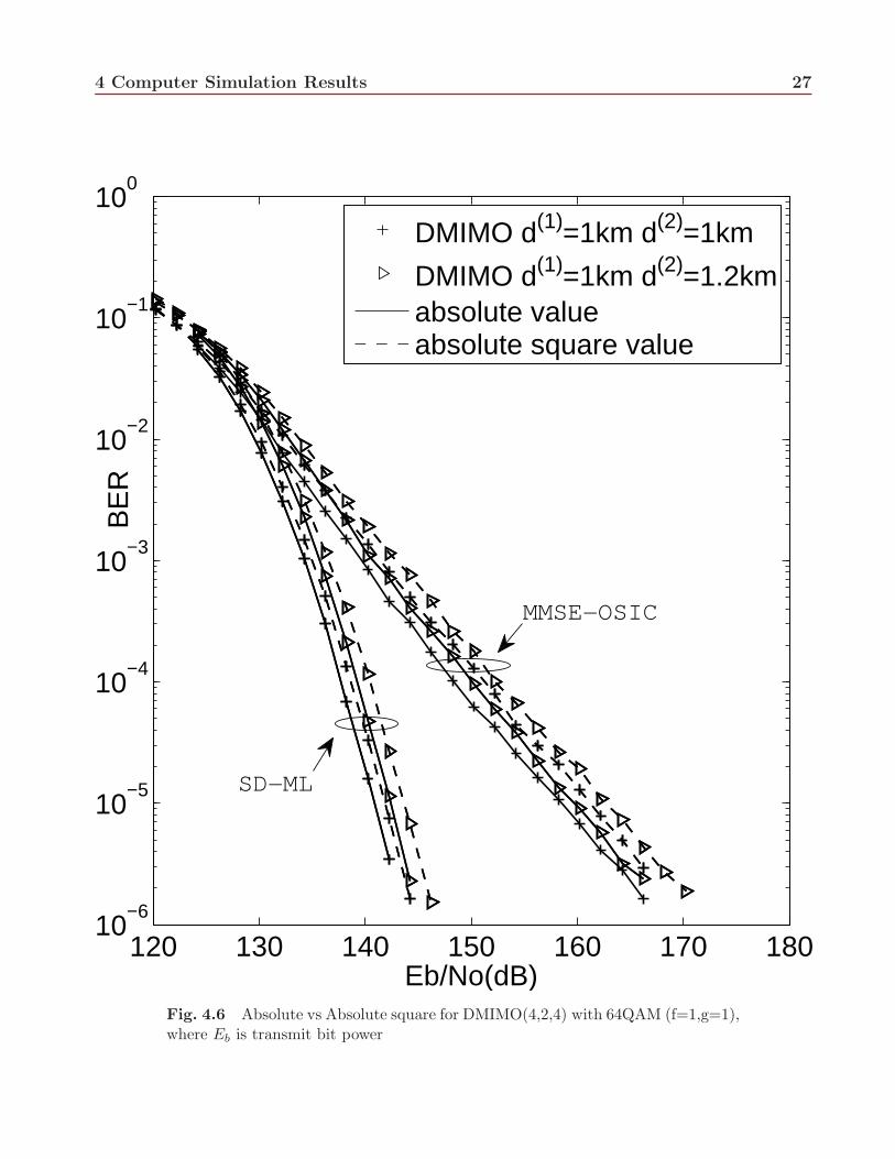
4.1 Simulations with Two Reliability Information Scheme
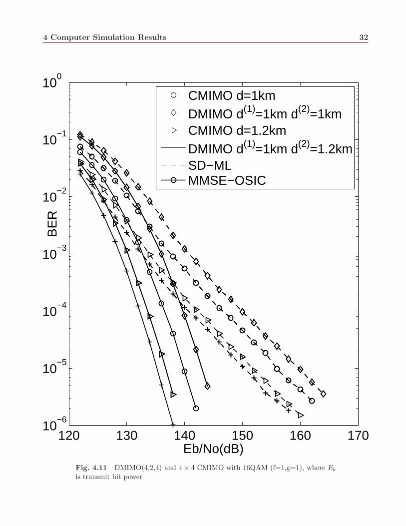
In this section, we present simulation results to show the effect of the reliability informationscheme on BER performance of D-MIMO. Two reliability information schemes are considered:reliability information with absolute value (3.25) and reliability information with absolute squarevalue (3.24). The considered modulation schemes are 16QAM, 32QAM and 64QAM. For eachmodulation scheme, parameter settings for the reliability information with f = 1, g = 1 andf = 0, g = 1 are considered. Two types of D-MIMO systems are considered: a (4,2,4) D-MIMOwith d(1) = d(2) = 1km and a (4,2,4) D-MIMO with d(1) = 1km, d(2) = 1.2km.
From Fig.4.2 ∼ Fig.4.7 we see that for all modulation schemes, the performance correspondingto reliability information based on absolute value is better than that based on absolute squarevalue. For SD-ML, the performance gain with reliability parameter settings f = 1, g = 1 (Fig4.2, Fig 4.4, Fig 4.6) is larger than that with f = 0, g = 1 (Fig 4.3, Fig 4.5, Fig 4.7), while forMMSE-OSIC, the performance gain with reliability parameter settings f = 0, g = 1 (Fig 4.3, Fig
4 Computer Simulation Results 18
0000000000
00001
00001
00010
00010
00011
00011
00100
00101
00110
00111
01000
01001
01010
01011
01100
01101
01110
01111
1000010000
10001
10001
10010
10010
10011
10011
10100
10101
10110
10111
11000
11001
11010
11011
11100
11101
11110
11111
Fig. 4.1 Construction of 32QAM from rectangular 32QAM
4.5, Fig 4.7) is larger than that with f = 1, g = 1 (Fig 4.2, Fig 4.4, Fig 4.6). At BER= 10−5,for SD-ML with reliability parameter settings f = 1, g = 1, the performance gain of reliabilityinformation with absolute value over that with absolute square value is 0.8dB, 1.0dB, 1.2dBfor 16QAM, 32QAM and 64QAM respectively, and for MMSE-OSIC with reliability parametersettings f = 0, g = 1, the performance gain of reliability information with absolute value over thatwith absolute square value is around 6.4dB, 5.3dB and 5.8dB for 16QAM, 32QAM and 64QAMrespectively. This varifies that our improvement of the reliability information scheme proposedin Chapter 3 provides gains, and this improvement has more significant effect on MMSE-OSICdetection scheme.
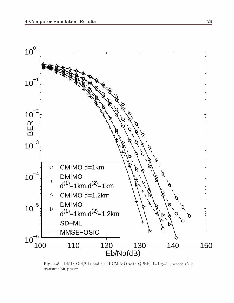
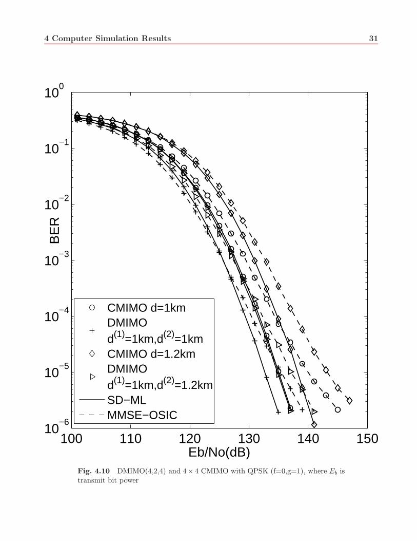
4.2 Simulations with Perfect Channel Information
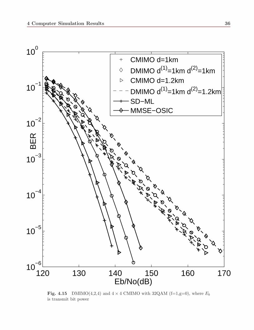
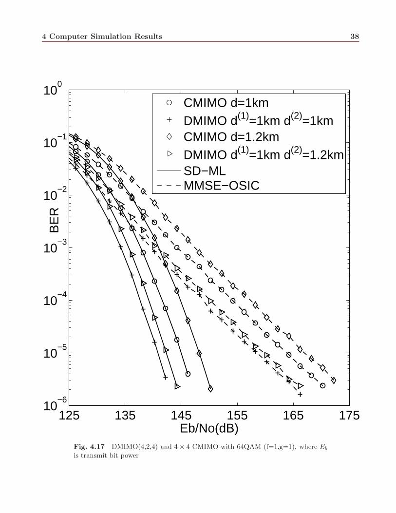
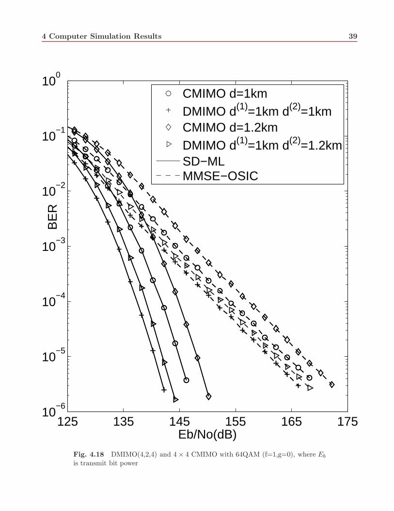
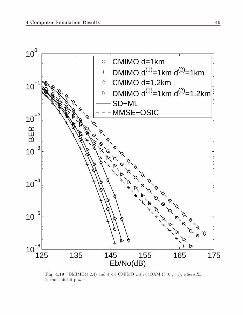
In this Section, we present simulation results of BER performance for uncorrelated D-MIMO andC-MIMO with perfect CSI. Fig 4.8, Fig 4.11, Fig 4.14, Fig 4.17 show the BER performance withreliability parameter settings f = 1, g = 1 for QPSK, 16QAM, 32QAM and 64QAM respectively.Fig 4.9, Fig 4.12, Fig 4.15, Fig 4.18 show the BER performance with reliability parameter settingsf = 1, g = 0 for QPSK, 16QAM, 32QAM and 64QAM respectively. Fig 4.10, Fig 4.13, Fig 4.16,Fig 4.19 show the BER performance with reliability parameter settings f = 0, g = 1 for QPSK,16QAM, 32QAM and 64QAM respectively. In all schemes, we present BER performance forthe following two kinds of D-MIMO systems: a (4,2,4) D-MIMO with d(1) = d(2) = 1km and a(4,2,4) D-MIMO with d(1) = 1km, d(2) = 1.2km, we also present results for two kinds of C-MIMOsystems: a 4 × 4 C-MIMO with d = 1km and a 4 × 4 C-MIMO with d = 1.2km.
We see that reliability parameter settings f and g play an important role on the performanceof D-MIMO with different detection schemes. According to Fig 4.9, Fig 4.12, Fig 4.15, Fig4.18, we see that for SD-ML with reliability parameter settings f = 1, g = 0, D-MIMO withd(1) = 1km, d(2) = 1.2km not only outperforms C-MIMO with d = 1.2km but also outperforms
4 Computer Simulation Results 19
C-MIMO with d = 1km; according to Fig 4.10, Fig 4.13, Fig 4.16, Fig 4.19, we see that forSD-ML with reliability parameter settings f = 0, g = 1, the performance of D-MIMO withd(1) = 1km, d(2) = 1.2km is better than that of C-MIMO with d = 1.2km, but it is worse thanthat of C-MIMO with d = 1km. Furthermore, for all modulation schemes, the performancegains of D-MIMO with d(1) = d(2) = 1km over C-MIMO with d = 1km for SD-ML detection withf = 1, g = 0 are much larger than that with f = 0, g = 1. So for D-MIMO with SD-ML, theperformances with reliability parameter setting f = 1, g = 0 are much better than those withreliability parameter settings f = 0, g = 1. We also see that for all modulation schemes, theperformances with reliability parameter setting f = 1, g = 0 (Fig 4.9, Fig 4.12, Fig 4.15, Fig4.18) are similar to those with reliability parameter settings f = 1, g = 1 (Fig 4.8, Fig 4.11, Fig4.14, Fig 4.17). This implies that for D-MIMO with SD-ML detection in all modulation schemes,the effect of symbol level SNR has more significant effect on the performance.
According to Fig 4.10, Fig 4.13, Fig 4.16, Fig 4.19, we see that for MMSE-OSIC with reliabilityparameter settings f = 0, g = 1, D-MIMO with d(1) = 1km, d(2) = 1.2km has significant betterperformance than both C-MIMO with d = 1.2km and C-MIMO with d = 1km; according toFig 4.9, Fig 4.12, Fig 4.15, Fig 4.18, we see that for MMSE-OSIC with reliability parametersettings f = 1, g = 0, D-MIMO with d(1) = 1km, d(2) = 1.2km still provide some improvementover C-MIMO with d = 1.2km, but it doesn’t outperform C-MIMO with d = 1km significantly.Furthermore, the performance gains of D-MIMO with d(1) = d(2) = 1km over C-MIMO withd = 1km for MMSE-OSIC detection with f = 0, g = 1 are much larger than that with f =1, g = 0. So for D-MIMO with MMSE-OSIC, the performances with reliability parameter settingf = 0, g = 1 are much better than those with reliability parameter settings f = 1, g = 0. Wealso see that for all modulation schemes, the performances with reliability parameter settingsf = 0, g = 1 (Fig 4.10, Fig 4.13, Fig 4.16, Fig 4.19) are a bit better than those with reliability
parameter settings f = 1, g = 1 (Fig 4.8, Fig 4.11, Fig 4.14, Fig 4.17) in the region of highEb
No
.
This implies that for D-MIMO with MMSE-OSIC detection the bit level reliability weight hasmore significant effect on the performance.
At BER= 10−5, the performance gains of a (4,2,4) D-MIMO over a 4 × 4 C-MIMO for SD-ML detection with reliability parameter settings f = 1, g = 0 (Fig 4.9, Fig 4.12, Fig 4.15, Fig4.18) corresponding to different modulation schemes are presented in Table 4.1. We see that theperformance gain for QPSK is a bit higher compared with the other three modulation schemes,and the performance gains for 16QAM, 32QAM and 64QAM are almost same which indicatesthat the performance improvment for D-MIMO with SD-ML is maintained as modulation sizeincreases. At BER= 10−5, the performance gains of a (4,2,4) D-MIMO over a 4 × 4 C-MIMOfor MMSE-OSIC with reliability parameter settings f = 0, g = 1 (Fig 4.10, Fig 4.13, Fig 4.16,Fig 4.19) corresponding to different modulation schemes are presented in Table 4.2. We see thatthe performance gain for QPSK is smaller compared with the other three modulation schemes.The performance gain for 16QAM is larger than that for 32QAM, and the performance gain for32QAM is larger than that for 64QAM. This indicates that the performance improvement forD-MIMO with MMSE-OSIC decreases when modulation size increases.
According to Table 4.1 and Table 4.2, we see that for both detection schemes, the performanceimprovement of D-MIMO with d(1) = 1km, d(2) = 1.2km over C-MIMO with d = 1.2km is greaterthan that of D-MIMO with d(1) = d(2) = 1km over C-MIMO with d = 1km, and the performanceimprovement of D-MIMO with d(1) = 1km, d(2) = 1.2km over C-MIMO with d = 1km is less
Table 4.2 The performance gain of D-MIMO over C-MIMO for MMSE-OSICwith f = 0, g = 1 at BER= 10−5
than that of D-MIMO with d(1) = d(2) = 1km over C-MIMO with d = 1km. Furthermore, for16QAM, 32QAM and 64QAM, the performance improvement of D-MIMO over C-MIMO forMMSE-OSIC with f = 0, g = 1 is larger than that for SD-ML with f = 1, g = 0.
4.3 Impact of Channel Estimation Errors
In this section, we consider the effect of channel estimation errors on the performance of D-
MIMO. Assume an L×M channel estimation matrix H(n)
, associated with the link between MSand Portn, as modeled in [33]:
H(n)
= H(n) + H(n)
(4.1)
where H(n) is the true channel matrix from MS to Portn, H(n)
is an L×M error matrix associatedwith Portn which is independent of H(n) and with i.i.d. CN (0, γ2σ2
n) entries, and γ2 is a constantindicating the relative error power with respect to the channel noise.
We consider two kinds of D-MIMO systems: a (4,2,4) D-MIMO with d(1) = d(2) = 1kmand a (4,2,4) D-MIMO with d(1) = 1km, d(2) = 1.2km, we also consider two kinds of C-MIMOsystems: a 4×4 C-MIMO with d = 1km and a 4×4 C-MIMO with d = 1.2km. Two modulationschemes are considered: 16QAM and 64QAM, both with Gray mapping. Two detection schemesare considered: SD-ML with reliability parameter settings f = 1, g = 0 and MMSE-OSIC with
4 Computer Simulation Results 21
reliability parameter settings f = 0, g = 1.Fig 4.20 ∼ Fig 4.27 present the BER performance with different values of γ2 for SD-ML and
MMSE-OSIC respectively. We observe that for all schemes, the performance improvement of D-MIMO over C-MIMO is maintained. The channel estimation error results in some degradationsin performance, which increases with γ2, and the degradations with a given channel estimationerror level γ2 are almost same for all modulation schemes. With SD-ML (Fig 4.20 ∼ Fig 4.23),at BER=10−5, the degradations are about 3dB for γ2 = 1 and about 10.3dB for γ2 = 10. WithMMSE-OSIC (Fig 4.24 ∼ Fig 4.27), at BER=10−5, the degradations are about 3dB for γ2 = 1and about 13dB for γ2 = 10.
4.4 Impact of Channel Spatial Correlation
In this section, we investigate the impact of channel spatial correlation on the performance ofD-MIMO. We consider a (4,2,4) D-MIMO system with d(1) = d(2) = 1km and a 4 × 4 C-MIMOwith d = 1km. The detection scheme is SD-ML with f = 1, g = 0. Three situations forspatial correlation are considered: spatial correlation at transmitter only, spatial correlation atreceiver only and spatial correlation at both transmitter and receiver. The channel model forspatial correlation employed is decribed in Chapter 2 (2.16), with R
(n)R and RT indicating the
receive correlation matrix at Portn (2.8) and transmit correlation matrix (2.5) respectively. Twomodulation schemes are considered: 16QAM and 64QAM, both with Gray mapping. We foundthat for both modulation schemes, performance with spatial correlation at receiver only is veryclose to that with spatial correlation at transmitter only, hence we do not include the resultswith spatial correlation at receiver only.
Fig. 4.28 ∼ Fig. 4.29 present the BER performance with correlation coefficient of 0.6 for16QAM and 64QAM respectively. We see that for both 16QAM and 64QAM, performanceimprovement of D-MIMO over C-MIMO is maintained. At BER=10−5, the improvement isaround 4.6dB for no space correlation, 4.2dB for space correlation at transmitter only and 3.8dBfor space correlation at both transmitter and receiver. We also observe that for both 16QAM and64QAM channel spatial correlation results in some degradations in performance, that increasesas space correlation increases.
4.5 Comparision between a (M,N,L) D-MIMO system and a M ×NL
C-MIMO system
In this section, we present simulation results for a (4,2,4) D-MIMO system with d(1) = d(2) = 1kmand a 4 × 8 C-MIMO system with d = 1km. Hence both systems have the same number oftransmit and receive antennas. We consider 16QAM with Gray code mapping and SD-MLdetection with f = 1, g = 0. The correlation coefficient in (2.5) and (2.8) in a given wave-field[34] is approximated as,
r(d) ≈ exp(−23Λ2d2) (4.2)
where Λ is the angular spread according to [34], d is the distance in wavelengths between twoantennas [27]. Assume uniform linear arrays at receiver with equidistant antenna spacing. Thenfor a 4× 8 C-MIMO system,using (4.2), we have when doubling the number of receive antennas
4 Computer Simulation Results 22
in the same space,r′ = exp(−23Λ2 · (d2/4)) = r
1/4. (4.3)
Fig(4.30) presents the BER performance for a (4,2,4) D-MIMO and a 4 × 8 C-MIMO withand without space correlation, where the same correlations at transmitter and receiver for bothD-MIMO and C-MIMO are considered. We see that the performance of an uncorrelated 4×8 C-MIMO is better than an uncorrelated (4,2,4) D-MIMO and the difference is 2.1dB at BER= 10−5.Performance for both C-MIMO and D-MIMO becomes worse as spatial correlation increases.When there is same spatial correlation at both transmitter and receiver, the performance ofC-MIMO is better than that of D-MIMO and the difference increases as spatial correlationincreases. At BER= 10−5, the difference is 2.5dB when t = r = 0.3, 2.92dB when t = r = 0.5 and3.75dB when t = r = 0.8. In this case, the detection scheme for a 4 × 8 C-MIMO is equivalentto implement a joint symbol detection of eight receive antennas from two base stations, whichneeds perfect channel state information (CSI) of two base stations together. According to thesystem assumption in Chapter 2, each base station only has its own perfect CSI. Hence, in orderto get perfect CSI for both base stations, connections between two basestations are requiredto exchange their CSI. However, such operations lead to large amount of information transferand increase the complexity and load of receiver. Hence, for case of same space correlation atreceiver, although the performance of a M × NL C-MIMO is better than a (M,N,L) D-MIMO,more complexity and heavier load are required at receiver of C-MIMO.
Fig(4.31) presents the BER performance for a (4,2,4) D-MIMO and a 4×8 C-MIMO with andwithout space correlation, where the same space restrictions at the receiver of C-MIMO and theradio ports of D-MIMO are considered. In this case, the detection scheme for a 4 × 8 C-MIMOis equivalent to implement a joint symbol detection of eight receiver antennas amounted on onebase station, which has the same space restriction to that of D-MIMO. Hence, space correlationat receiver is higher for a 4 × 8 C-MIMO (4.3) than for a (4,2,4) D-MIMO. With same spacecorrelation at transmitter for both 4 × 8 C-MIMO and (4,2,4) D-MIMO, the performance ofC-MIMO is a bit better than that of D-MIMO and the difference decreases as spatial correlationincreases. At BER= 10−5, the difference between C-MIMO with t = 0.3, r = 0.74 and D-MIMO with t = r = 0.3 is 0.43dB, the difference between C-MIMO with t = 0.5, r = 0.84and D-MIMO with t = r = 0.5 is 0.26dB and the performance of D-MIMO with t = r = 0.8is slightly better than that of C-MIMO with t = 0.8, r = 0.95. Simulation results verify thatin realistic systems with restricted space at receiver, space correlation among antennas is animportant factor. The proposed bit combining scheme for a (M,N,L) D-MIMO system providesa comparable performance to a M ×NL C-MIMO system with complexity suitable for practicalapplications, especially when space correlation increases.
4 Computer Simulation Results 23
120 130 140 150 160 17010
−6
10−5
10−4
10−3
10−2
10−1
100
Eb/No(dB)
BE
R
DMIMO d(1)=1km d(2)=1km
DMIMO d(1)=1km d(2)=1.2kmabsolute valueabsolute square value
MMSE−OSIC
SD−ML
Fig. 4.2 Absolute vs Absolute square for DMIMO(4,2,4) with 16QAM (f=1,g=1),where Eb is transmit bit power
4 Computer Simulation Results 24
120 130 140 150 160 17010
−6
10−5
10−4
10−3
10−2
10−1
100
Eb/No(dB)
BE
R
DMIMO d(1)=1km d(2)=1km
DMIMO d(1)=1km d(2)=1.2kmabsolute valueabsolute square value
SD−ML
MMSE−OSIC
Fig. 4.3 Absolute vs Absolute square for DMIMO(4,2,4) with 16QAM (f=0,g=1),where Eb is transmit bit power
4 Computer Simulation Results 25
120 130 140 150 160 17010
−6
10−5
10−4
10−3
10−2
10−1
100
Eb/No(dB)
BE
R
DMIMO d(1)=1km d(2)=1km
DMIMO d(1)=1km d(2)=1.2kmabsolute valueabsolute square value
SD−ML
MMSE−OSIC
Fig. 4.4 Absolute vs Absolute square for DMIMO(4,2,4) with 32QAM (f=1,g=1),where Eb is transmit bit power
4 Computer Simulation Results 26
120 130 140 150 160 17010
−6
10−5
10−4
10−3
10−2
10−1
100
Eb/No(dB)
BE
R
DMIMO d(1)=1km d(2)=1km
DMIMO d(1)=1km d(2)=1.2kmabsolute valueabsolute square value
SD−ML
MMSE−OSIC
Fig. 4.5 Absolute vs Absolute square for DMIMO(4,2,4) with 32QAM (f=0,g=1),where Eb is transmit bit power
4 Computer Simulation Results 27
120 130 140 150 160 170 18010
−6
10−5
10−4
10−3
10−2
10−1
100
Eb/No(dB)
BE
R
DMIMO d(1)=1km d(2)=1km
DMIMO d(1)=1km d(2)=1.2kmabsolute valueabsolute square value
MMSE−OSIC
SD−ML
Fig. 4.6 Absolute vs Absolute square for DMIMO(4,2,4) with 64QAM (f=1,g=1),where Eb is transmit bit power
4 Computer Simulation Results 28
120 130 140 150 160 170 18010
−6
10−5
10−4
10−3
10−2
10−1
100
Eb/No(dB)
BE
R
DMIMO d(1)=1km d(2)=1km
DMIMO d(1)=1km d(2)=1.2kmabsolute valueabsolute square value
MMSE−OSIC
SD−ML
Fig. 4.7 Absolute vs Absolute square for DMIMO(4,2,4) with 64QAM (f=0,g=1),where Eb is transmit bit power
Fig. 4.21 Effect of channel estimation error: DMIMO(4,2,4) d(1) = 1km, d(2) =1.2km and 4× 4 CMIMO d=1.2km with SD-ML for 16QAM, where Eb is transmitbit power
4 Computer Simulation Results 43
125 135 145 155 16510
−6
10−5
10−4
10−3
10−2
10−1
100
Eb/No(dB)
BE
R
CMIMO d=1kmDMIMO d(1)=1km d(2)=1kmSD−MLSD−ML γ2=1
SD−ML γ2=10
Fig. 4.22 Effect of channel estimation error: DMIMO(4,2,4) d(1) = d(2) = 1kmand 4×4 CMIMO d=1km with SD-ML for 64QAM, where Eb is transmit bit power
Fig. 4.23 Effect of channel estimation error: DMIMO(4,2,4) d(1) = 1km, d(2) =1.2km and 4× 4 CMIMO d=1.2km with SD-ML for 64QAM, where Eb is transmitbit power
Fig. 4.24 Effect of channel estimation error: DMIMO(4,2,4) d(1) = d(2) = 1kmand 4 × 4 CMIMO d=1km with MMSE-OSIC for 16QAM, where Eb is transmitbit power
Fig. 4.25 Effect of channel estimation error: DMIMO(4,2,4) d(1) = 1km, d(2) =1.2km and 4 × 4 CMIMO d=1.2km with MMSE-OSIC for 16QAM, where Eb istransmit bit power
Fig. 4.26 Effect of channel estimation error: DMIMO(4,2,4) d(1) = d(2) = 1kmand 4 × 4 CMIMO d=1km with MMSE-OSIC for 64QAM, where Eb is transmitbit power
Fig. 4.27 Effect of channel estimation error: DMIMO(4,2,4) d(1) = 1km, d(2) =1.2km and 4 × 4 CMIMO d=1.2km with MMSE-OSIC for 64QAM, where Eb istransmit bit power
Fig. 4.28 Effect of channel spatial correlation: DMIMO(4,2,4) d(1) = d(2) = 1kmand 4×4 CMIMO d=1km with SD-ML for 16QAM, where Eb is transmit bit power
Fig. 4.29 Effect of channel spatial correlation: DMIMO(4,2,4) d(1) = d(2) = 1kmand 4×4 CMIMO d=1km with SD-ML for 64QAM, where Eb is transmit bit power
4 Computer Simulation Results 51
120 125 130 135 140 145 15010
−7
10−6
10−5
10−4
10−3
10−2
10−1
100
Eb/No(dB)
BE
R
C t=r=0D t=r=0C t=r=0.3D t=r=0.3C t=r=0.5D t=r=0.5C t=r=0.8D t=r=0.8
Fig. 4.30 Same space correlation for DMIMO(4,2,4) d(1) = d(2) = 1km (’D’ inlegend) and 4× 8 CMIMO d=1km (’C’ in legend) with SD-ML for 16QAM, whereEb is transmit bit power
Fig. 4.31 Same space constraint at receiver of DMIMO(4,2,4) d(1) = d(2) = 1km(’D’ in legend) and 4× 8 CMIMO d=1km (’C’ in legend) with SD-ML for 16QAM,where Eb is transmit bit power
53
Chapter 5: D-MIMO Performance Analysis
In the previous chapter, we analyzed the BER performance of D-MIMO by using Monte-Carlosimulations. In this chapter, we present theoretical BER performance analysis for D-MIMOsystem. We consider a D-MIMO system with two base stations where bk ∈ {0, 1} is the kthtransmitted bit, k = 1, . . . ,MQ0. According to the bit level combining scheme implemented inthe Fusion Center (3.6)(3.7), the error probability for the kth bit of D-MIMO is:
Pr(ˆbk 6= bk) = Pr[(−1)b
(1)k w
(1)k + (−1)b
(2)k w
(2)k > 0|bk = 1] · Pr(bk = 1)
+ Pr[(−1)b(1)k w
(1)k + (−1)b
(2)k w
(2)k < 0|bk = 0] · Pr(bk = 0)
= A · Pr(bk = 1) +B · Pr(bk = 0) (5.1)
where w(n)k ≥ 0 is the kth element of w(n) (3.27), and
A = Pr[(−1)b(1)k w
(1)k + (−1)b
(2)k w
(2)k > 0|bk = 1] = A00 + A01 + A10 + A11. (5.2)
We have
A00 = Pr[w(1)k + w
(2)k > 0|bk = 1, b
(1)k = 0, b
(2)k = 0] · Pr(b(1)k = 0, b
(2)k = 0|bk = 1)
= Pr(b(1)k = 0|bk = 1)Pr(b
(2)k = 0|bk = 1) = p
(1)k · p(2)
k (5.3)
where the second equality is because b(1)k and b
(2)k are independent, w
(1)k , w
(2)k are positive with
probability 1, and p(n)k is the probability that b
(n)k is in error. Similarly, we have:
A01 = Pr[w(1)k − w
(2)k > 0|bk = 1, b
(1)k = 0, b
(2)k = 1] · Pr(b(1)k = 0, b
(2)k = 1|bk = 1)
= Pr[w(1)k − w
(2)k > 0|bk = 1, b
(1)k = 0, b
(2)k = 1] · p(1)
k · (1 − p(2)k ) (5.4)
A10 = Pr[w(1)k − w
(2)k < 0|bk = 1, b
(1)k = 1, b
(2)k = 0] · Pr(b(1)k = 1, b
(2)k = 0|bk = 1)
= Pr[w(1)k − w
(2)k < 0|bk = 1, b
(1)k = 1, b
(2)k = 0] · (1 − p
(1)k ) · p(2)
k (5.5)
A11 = Pr[−w(1)k − w
(2)k > 0|bk = 1, b
(1)k = 1, b
(2)k = 1] · Pr(b(1)k = 1, b
(2)k = 1|bk = 1) = 0 (5.6)
since w(1)k , w
(2)k cannot be negative. Similarly, we have
B = Pr[(−1)b(1)k w
(1)k + (−1)b
(2)k w
(2)k < 0|bk = 0] = B00 +B01 +B10 +B11 (5.7)
B00 = Pr[w(1)k + w
(2)k < 0|bk = 0, b
(1)k = 0, b
(2)k = 0] · Pr(b(1)k = 0, b
(2)k = 0|bk = 0) = 0 (5.8)
B01 = Pr[w(1)k − w
(2)k < 0|bk = 0, b
(1)k = 0, b
(2)k = 1] · Pr(b(1)k = 0, b
(2)k = 1|bk = 0)
= Pr[w(1)k − w
(2)k < 0|bk = 0, b
(1)k = 0, b
(2)k = 1] · (1 − p
(1)k ) · p(2)
k (5.9)
B10 = Pr[w(1)k − w
(2)k > 0|bk = 0, b
(1)k = 1, b
(2)k = 0] · Pr(b(1)k = 1, b
(2)k = 0|bk = 0)
= Pr[w(1)k − w
(2)k > 0|bk = 0, b
(1)k = 1, b
(2)k = 0] · p(1)
k · (1 − p(2)k ) (5.10)
B11 = Pr[−w(1)k − w
(2)k < 0|bk = 0, b
(1)k = 1, b
(2)k = 1] · Pr(b(1)k = 1, b
(2)k = 1|bk = 0)
= p(1)k · p(2)
k (5.11)
5 D-MIMO Performance Analysis 54
Since w(n)k , the bit reliability information, is related to the type of MIMO detection employed
at the Ports, we analyze the BER performance of D-MIMO based on the type of MIMO detectionemployed. In this thesis, we analyze the BER performance of D-MIMO with SD-ML detection.
5.1 Performance Analysis for C-MIMO with SD-ML Detection
To analyze BER performance of D-MIMO, we need to first find out p(n)k , the probability of
bit error for C-MIMO over a composite Rayleigh-lognormal environment. According to [9], thepairwise error probability (PEP) that the receiver mistakes the transmitted signal vector si foranother signal vector sj in an L×M MIMO system with SD-ML detection scheme is:
P (si → sj |H, si) = Q
(√
‖Hdij‖2
2σ2n
)
(5.12)
where dij = si − sj . Based on channel model (2.16), ‖Hdij‖2 = |hsh(d)|2 · ‖Hssfdij‖2. LetW = |hsh(d)|2 and V = ‖Hssfdij‖2, due to the independence of W and V , the average PEP is:
PEPavg = EW
[
EV
[
Q
(√
W · V2σ2
n
)]]
(5.13)
Let a = Hssfdij, since Hssf = R1/2R HwR
1/2T with Hw an L ×M matrix with i.i.d. CN (0, 1)
entries. Then a is complex normal distributed with mean vector E[a] = 0. Define R1/2T dij =
u = [u1, . . . , uM ]T . We have ‖R1/2T dij‖2 =
∑Mi=1 |ui|2. Then the covariance matrix:
Ra = E[aaH ] = E[
R1/2R HwR
1/2T dij · dH
ij (R1/2T )HHH
w (R1/2R )H
]
= R1/2R E
[HwuuHHH
w
](R
1/2R )H = R
1/2R E
[M∑
i=1
(hw)iui ·M∑
j=1
(hw)Hj u
∗j
]
(R1/2R )H
= R1/2R · I
M∑
i=1
|ui|2 · (R1/2R )H = ‖R1/2
T dij‖2 · RR (5.14)
where we used E[(hw)i · (hw)H
j
]=
{I i = j0 i 6= j
.
Since V = ‖a‖2 = aHQa is a Hermitian quadratic form in zero mean complex Gaussianrandom variables, where Q = I, we have the characteristic function of random variable V [35]:
ϕV (z) =1
det(I− z · Ra)=
1∏L
k=1(1 − zζk)(5.15)
where ζk are the eigenvalues of Ra. According to the receive correlation matrix model in Chapter2, the Hermitian matrix RR is positive definite, making the Hermitian matrix Ra is also positivedefinite, and hence, ζk are positive.
With the representation of the Q function obtained by Craig [36], we have:
Q
(√
W · V2σ2
n
)
=1
π
∫ π2
0
exp
[
− 1
2 sin2(φ)· W · V
2σ2n
]
dφ, (5.16)
5 D-MIMO Performance Analysis 55
and the first expectation in (5.13) becomes
EV
[
Q
(√
W · V2σ2
n
)]
=1
π
∫ π2
0
EV
[
exp
(
− W · V4 sin2(φ) · σ2
n
)]
dφ
=1
π
∫ π2
0
ϕV
(
− W
4 sin2(φ) · σ2n
)
dφ =1
π
∫ π2
0
1∏L
k=1
(
1 + W ·ζk
4σ2n sin2(φ)
)dφ. (5.17)
where the last equality is obtained using (5.15). To solve the integration in (5.17), we need to
perform partial fraction expension for rational function1
∏Lk=1
(1 + ck
x
) , where ck =Wζk4σ2
n
and
x = sin2(φ). The complete derivation of partial fraction expension is provided in Appendix A.
5.1.1 PEP in case of spatial correlation at receiver
In case of spatial correlation at receiver, RR is a Hermitian Toeplitz matrix. By using functioneig(·) in matlab to get eigenvalues of a 4 × 4 receive correlation matrix with different fadingcorrelation coefficient r = 0.1, . . . , 0.9, we find that the eigenvalues of each test are distinct. Fur-thermore, [37] mentioned that for a matrix with Hermitian Toeplitz structure, the eigenvalues areseldomly exactly equal. This leads to assume Hermitian Toeplitz matrix Ra has distinct eigenval-
ues ζk, k = 1, . . . , L, then the intergrand of (5.17)1
∏Lk=1
(
1 + W ·ζk
4σ2n sin2(φ)
) has L simple poles, with
partial fraction expansion (A.1):1
∏Lk=1
(
1 + W ·ζk
4σ2n sin2(φ)
) = 1+L∑
i=1
(−ci)L
∏Lk=1,k 6=i(ck − ci)(sin
2(φ) + ci),
where ck =Wζk4σ2
n
. The PEP averaged over small scale fading (5.17) will be:
EV
[
Q
(√
W · V2σ2
n
)]
=1
π
(
π
2+
L∑
i=1
(−ci)L
∏Lk=1,k 6=i(ck − ci)
∫ π2
0
1
sin2(φ) + cidφ
)
(5.18)
where
∫ π2
0
1
sin2(φ) + cidφ =
∫ π2
0
112
+ ci − 12cos(2φ)
dφ =1
2
∫ π
0
112
+ ci − 12cos t
dt =π
2√
c2i + ci(5.19)
where the first equality is because of sin2(φ) =1
2(1−cos(2φ)) and the third equality is according
to [38] (eq.3.661.4). With (5.19) and substitution of ck =Wζk4σ2
n
, (5.18) will be:
EV
[
Q
(√
W · V2σ2
n
)]
=1
2
(
1 +
L∑
i=1
(−ci)L
∏Lk=1,k 6=i(ck − ci)
· 1√
c2i + ci
)
=1
2
(
1 +L∑
i=1
(−ζi)L
∏Lk=1,k 6=i(ζk − ζi)
·√
W
ζ2i ·W + 4σ2
nζi
)
(5.20)
According to (2.13) in Chapter 2, we have:
W = |hsh(d)|2 =κ · φdτ
(5.21)
5 D-MIMO Performance Analysis 56
where 10 log10 φ ∼ N (0, σ2φdB
). Taking the logarithm of (5.21) we have:
10 log10 W = 10 log10(κ
dτ) + 10 log10 φ = µ+ 10 log10 φ (5.22)
where µ = 10 log10(κ
dτ) is a constant and we have: 10 log10W ∼ N (µ, σ2
φdB) ⇒ lnW ∼
N (λµ, (λσφdB)2), where λ =
ln 10
10. So random variable W is log-normally distributed with
pdf:fW (w) =
1√2π(λσφdB
)wexp
[
−(lnw − λµ)2
2(λσφdB)2
]
w > 0. (5.23)
Then the average PEP including large-scale fading (shadowing) is:
PEPavg = EW
[
EV
[
Q
(√
W · V2σ2
n
)]]
=
∫ ∞
0
EV
[
Q
(√
w · V2σ2
n
)]
· fW (w)dw
=1
2+
1
2
L∑
i=1
(−ζi)L
∏Lk=1,k 6=i(ζk − ζi)
∫ ∞
0
√w
ζ2i · w + 4σ2
nζifW (w)dw, (5.24)
where∫ ∞
0
√w
ζ2i · w + 4σ2
nζifW (w)dw =
1√2π(λσφdB
)
∫ ∞
0
√
1
ζ2i w
2 + 4σ2nζiw
exp
[
−(lnw − λµ)2
2(λσφdB)2
]
dw
=1√2π
∫ ∞
−∞
√
exp(λσφdBt+ λµ)
ζ2i · exp(λσφdB
t+ λµ) + 4σ2nζi
· exp
(
−t2
2
)
dt (5.25)
in the second equality we use the substitution t =lnw − λµ
λσφdB
.
Using Gauss-Hermite integration
∫ ∞
−∞
e−x2
f(x)dx =n∑
p=1
wpf(xp) where n is the order of
Hermite polynomials, xp are the zeros of Hermite polynomials and wp are the weights [39], then
PEPavg =1
2+
1
2√π
L∑
i=1
(−ζi)L
∏Lk=1,k 6=i(ζk − ζi)
n∑
p=1
wp
√
exp (λσφdB·√
2xp + λµ)
ζ2i exp (λσφdB
·√
2xp + λµ) + 4σ2nζi
(5.26)
5.1.2 PEP in case of no spatial correlation at receiver
In case of no spatial correlation at receiver, covariance matrix Ra has an eigenvalue ζ =
‖R1/2T dij‖2 with multiplicity L, the integrand in (5.17) will be
1(
1 + W ·ζ4σ2
n sin2(φ)
)Lwhich is a func-
tion with a pole at −W · ζ4σ2
n
of order L. Let c =W · ζ4σ2
n
, its partial fraction expansion (A.3) is:
1(
1 + W ·ζ4σ2
n sin2(φ)
)L= 1 +
L∑
i=1
(Li
)(−c)i
(sin2(φ) + c)i. The PEP averaged over small scale fading (5.17) is:
EV
[
Q
(√
W · V2σ2
n
)]
=1
π
(
π
2+
L∑
i=1
(L
i
)
(−c)i
∫ π2
0
1
(sin2(φ) + c)idφ
)
(5.27)
5 D-MIMO Performance Analysis 57
Similarly, according to [38] (eq.3.661.4), we have:∫ π
2
0
1
(sin2(φ) + c)idφ =
∫ π2
0
1
(12
+ c− 12cos(2φ))i
dφ =1
2
∫ π
0
1
(12
+ c− 12cos t)i
dt
=π
2· 1
(2c)i−1√c2 + c
i−1∑
k=0
(2(i− 1) − 2k − 1)!!(2k − 1)!!
(i− 1 − k)!k!·(
c
1 + c
)k
(5.28)
where (2n− 1)!! =∏n
i=1(2i− 1), (−1)!! = 1. Let j = i− 1 and substitude (5.28) in (5.27), then:
EV
[
Q
(√
W · V2σ2
n
)]
=1
2
[
1 +
L−1∑
j=0
(L
j + 1
)(−c)j+1
(2c)j√c2 + c
j∑
k=0
(2j − 2k − 1)!!(2k − 1)!!
(j − k)!k!·(
c
1 + c
)k]
=1
2
[
1 +
L−1∑
j=0
j∑
k=0
(L
j + 1
)
(−1)j+1
(1
2
)j(2j − 2k − 1)!!(2k − 1)!!
(j − k)!k!·(
Wζ
4σ2n +Wζ
)k+ 12
]
(5.29)
And the average PEP including large scale fading is:
PEPavg = EW
[
EV
[
Q
(√
W · V2σ2
n
)]]
=1
2+
1
2
L−1∑
j=0
j∑
k=0
(L
j + 1
)
(−1)j+1
(1
2
)j
·
(2j − 2k − 1)!!(2k − 1)!!
(j − k)!k!·∫ ∞
0
(wζ
4σ2n + wζ
)k+ 12
fW (w)dw (5.30)
where∫ ∞
0
(wζ
4σ2n + wζ
)k+ 12
fW (w)dw =1√
2π(λσφdB)
∫ ∞
0
(wζ
4σ2n + wζ
)k+ 12
· 1
wexp
[
−(lnw − λµ)2
2(λσφdB)2
]
dw
=1√2π
∫ ∞
−∞
(ζ · exp(λσφdB
t+ λµ)
4σ2n + ζ · exp(λσφdB
t+ λµ)
)k+ 12
· exp
(
−t2
2
)
dt (5.31)
Using Gauss-Hermite integration and with (5.31) we have
PEPavg =1
2+
1
2√π
L−1∑
j=0
j∑
k=0
(L
j + 1
)
(−1)j+1
(1
2
)j(2j − 2k − 1)!!(2k − 1)!!
(j − k)!k!·
n∑
p=1
wp
(
ζ · exp(λσφdB
√2xp + λµ)
4σ2n + ζ · exp(λσφdB
√2xp + λµ)
)k+ 12
. (5.32)
We have σ2n =
σ2s
γ=
1
M · γ . Numerical results show that n = 7 is enough to provide accurate
evaluation for PEPavg .
5.1.3 BER performance for C-MIMO over space uncorrelated channels
Consider the co-located MIMO system r = Hs + n, where s ∈ {s1, s2, . . . , sQM}. H is L ×Mcomposite fading channel matrix (2.16) with M ≤ L following Kronecker model,
H = hsh(d) · HSSF =√WR
1/2R HwR
1/2T (5.33)
5 D-MIMO Performance Analysis 58
where the small scale fading matrix HSSF = R1/2R HwR
1/2T with receive correlation matrix RR
and transmit correlation matrix RT deterministic and Hermitian [27], Hw is an L×M randommatrix with i.i.d complex Gaussian components. The shadowing coefficient
√W = hsh(d) is a
random variable with lognormal distribution.The conditional union bound on BER for a given transmit symbol vector si is [40]:
Pb,ub|W,Hw,si=
1
M · log2Q
QM∑
j=1,j 6=i
i(si, sj)P (si → sj|W,Hw, si) (5.34)
where i(si, sj) denotes the number of information bit errors corresponding to the pair of symbols(si, sj), P (si → sj |W,Hw, si) is the conditioned pairwise error probability (5.12) that receivermistakes transmit signal vector si for another signal vector sj for a given W , Hw and si.
Averaging (5.34) over Hw and W , and also over all possibilities of transmit symbol vector si,result in the average union bound on BER
Pb,ub =1
QM ·M · log2Q
QM∑
i=1
QM∑
j=1,j 6=i
i(si, sj)P (si → sj |si) (5.35)
where P (si → sj|si) is the average PEP over a composite Rayleigh-lognormal channel H (5.13).
BER evaluation technique for uncorrelated channels
For uncorrelated channels, the average PEP, obtained by using (5.32), is a function of ‖dij‖2
where dij = si − sj. Let d1 < d2 <, . . . , < dMmax be the distance spectrum of ‖dij‖. The doublesum in (5.35) can be simplified by using a transfer function approach [40],
Pb,ub =1
QM ·M · log2Q
Mmax∑
m=1
a(m)P2(dm) (5.36)
where Mmax indicates the largest Euclidean distance between si and sj, P2(dm) denotes av-erage PEP for uncorrlated channels, obtained by using (5.32) with ζ = d2
m, and a(m) =QM∑
i=1
QM∑
j=1,j 6=i
[i(si, sj)|(‖dij‖2 = d2m)] indicates the total number of information bit errors associ-
ated with a pair of symbol vectors satisfying ‖dij‖2 = d2m, that can be obtained by using the
transfer function [40],
a(m) =
[1
m!
dm
dDm
([d
dIT (D, I)
]
I=1
)]
D=0
. (5.37)
In [40], transfer functions for square QAM constellations with Gray code mapping are pre-sented. We extend the transfer function to a truncated square QAM constellation with quasi-Gray code mapping such as 32QAM in Appendix B. Table 5.1 shows the transfer function T (D, I)for QPSK, 16QAM, 32QAM and 64QAM respectively, with the assumption that same modula-tion schemes are used in all transmit antennas.
In Fig.(5.1), we see that the largest squared Euclidean distance between two signal pointsequals 2(
√Q− 1)2|dmin|2 for square QAM, and 34|dmin|2 for truncated 32QAM (solid line) with
dmin indicating the distance between two nearest neighbor symbols in the constellation. Letsk
i and skj be the kth component of si and sj respectively, k = 1, . . . ,M . Hence the largest
squared Euclidean distance between si and sj is the case that for all values of k, satisfying
Table 5.1 Transfer function for QPSK, 16QAM, 32QAM and 64QAM
32 QAM 16 QAM
Fig. 5.1 Largest Euclidean distance in 32 QAM and square QAM constellation
|ski − sk
j |2 =
{2(√Q− 1)2|dmin|2 square QAM
34|dmin|2 32QAM. Hence d2
Mmax= Mmax|dmin|2 with
Mmax =
{2M(
√Q− 1)2 square QAM constellation
34M 32 QAM(5.38)
The distance spectrum dm in 32QAM and a square QAM constellation can be expressed asd2
m = m|dmin|2, allowing a(m) = 0 for certain values of m.The union upper bound which is averaged over the composite fading channel H could be very
loose, especially at low SNR, since there is no dominant error event in PEP and many termscontribute significantly to the summations in (5.36). In [41], a much tighter upper bound isobtained by limiting the conditional union upper bound before averaging over H. However, dueto the minimization, the order of integration and summation cannot be changed and (ML+1)-foldintegration has to be carried out numerically, becomeing compuationally expensive. Furthermore,to obtain full union bound by computing all values of a(m) and P2(dm) for large number oftransmit antennas and symbol constellation size may be complex. Hence, we consider BERevaluation by using truncated union bound,
Pb =1
QM ·M · log2Q
K∑
m=1
a(m)P2(dm) K ≤Mmax (5.39)
K indicates the number of terms needed to evaluate the BER. Numerical results in the following
5 D-MIMO Performance Analysis 60
section show the values of K required for tight BER approximation at different ranges of BER.
Numerical Results
In this section, we present BER numerical evaluation and simulation results for uncorrelatedC-MIMO. In all schemes, BER is plotted versus Eb/No, where Eb is averaged receive bit power.
Computation of the average receive Eb/No
According to the composite fading channel model in Chapter 2 and considering the independenceof small-scale fading and large-scale fading, the averaged receive signal power on the j th receiveantenna is given by:
σ2s j = E
[M∑
i=1
M∑
k=1
hjih∗jksis
∗k
]
=M∑
i=1
M∑
k=1
E[hjih
∗jk
]E[sis
∗k]
=
M∑
i=1
E[|hji|2] ·PT
M=PT
M· E[h2
sh(d)] ·M∑
i=1
E[
|hji|2]
(5.40)
where hji is the small-scale fading coefficient from the ith transmit antenna to the j th receiveantenna, the second equality is because the independence of H from s, the third equality uses
E[sis∗k] =
{PT
Mi = k
0 i 6= k. According to (2.13), we have: E[h2
sh(d)] =κ
dτ·E[φ], indicating that the
large-scale fading gain is a function of d, the distance between transmitter and receiver. Sincelnφ ∼ N (0, (λσφdB
)2), with λ = ln 1010
, we have
E[φ] =
∫ ∞
0
xfφ(x)dx =
∫ ∞
0
1√2πλσφdB
exp
[
− (ln x)2
2(λσφdB)2
]
dx
=e
12(λσφdB
)2
√2πλσφdB
∫ ∞
−∞
exp
(
− 1
2(λσφdB)2
[t− (λσφdB)2]2)
dt
=e
12(λσφdB
)2
√2πλσφdB
∫ ∞
−∞
e− t′2
2(λσφdB)2 dt′ = e
12(λσφdB
)2 (5.41)
where we substitute ln x = t in the third equality, t′ = t − (λσφdB)2 in the fourth equality and
∫ ∞
−∞
e− t′2
2(λσφdB)2 dt′ =
√2πλσφdB
[38] (eq. 3.323.2). Assume d = 1000m and with parameters:
fc = 1.9GHz, d0 = 100m, τ = 4 and σφdB= 4, we have
According to (2.9), the small-scale fading matrix of C-MIMO is represented by a Kronecker
model, Hssf = R1/2R HwR
1/2T . Let ei be a unit vector with 1 in the ith position and 0 elsewhere.
Define R1/2T ei = g, we have ‖g‖2 = eH
i (R1/2T )HR
1/2T ei = (RT )ii = 1:
E[|hji|2] = E[eHj R
1/2R HwR
1/2T ei · eH
i (R1/2T )H(Hw)H(R
1/2R )Hej ]
= eHj R
1/2R · E[Hwg · gH(Hw)H ] · (R1/2
R )Hej = eHj R
1/2R ·E[
M∑
k=1
(hw)kgk ·M∑
l=1
(hw)Hl g
∗l ] · (R1/2
R )Hej
=M∑
k=1
|gk|2 · eHj R
1/2R (R
1/2R )Hej = ‖g‖2 · (RR)jj = 1 (5.43)
5 D-MIMO Performance Analysis 61
where we used E[(hw)k(hw)Hl ] =
{I k = l0 k 6= l
. Hence∑M
i=1E[
|h2ji
]
= M , and the averaged
receive symbol power on each receive antenna (5.40) will be:
σ2s j = σ2
s =PT
M·M ·E[h2
sh(d)] = PT · κdτ
· e 12(λσφdB
)2 (5.44)
andEb
No=
σ2s
Q0No.
Fig. (5.2) ∼ Fig. (5.7) present BER evaluation results for uncorrelated 2 × 2 C-MIMO withQPSK, 2× 2 C-MIMO with 16QAM, 4× 4 C-MIMO with QPSK, 4× 4 C-MIMO with 16QAM,2 × 4 C-MIMO with QPSK and 2 × 4 C-MIMO with 16QAM. For each system, the BER wasevaluated with different values of K (5.39). We see that BER results with K = 1 provides a lowerbound, becoming tighter as the number of receive antennas L increases, and becoming looser asthe size of constellation Q increases. BER evaluation results tend to converge as K increases,especially at range of low BER.
Fig. (5.8) ∼ Fig. (5.13) illustrate clearer the tightness of BER evaluations with differentvalues of K. In all figures, the solid lines denote the values of Eb/No required to achieve BER=10−2, BER= 10−4 and BER= 10−6 based on simulation results. Marker-”*”, marker-”+” andmarker-”x” stand for the required values of Eb/No based on (5.39) for different values of K toachieve BER= 10−2, BER= 10−4 and BER= 10−6 respectively. Considering the uncorrelated2 × 2 C-MIMO with 16QAM (Fig. 5.9), we see that BER evaluation with K = 2 provides tightapproximation at range of high BER, BER evaluations with K ≥ 5 provide tight approximationsat range of moderate-to-low BER. However, since the complexity of BER evaluation increasesas K increases, it seems that K = 5 is optimum to provide tight approximations at range ofmoderate-to-low BER. Furthermore, K = 3 provides good approximation for whole range ofBER. Similar analysis (Table. 5.2) can be extended to other C-MIMO systems presented in Fig.(5.8) ∼ Fig. (5.13).
high BER moderate BER low BER full BER range2 × 2 QPSK 2 2 2 22 × 2 16QAM 2 5 5 34 × 4 QPSK 2 3 4 34 × 4 16QAM 2 4 7 32 × 4 QPSK 1 2 2 22 × 4 16QAM 1 2 2 2
Table 5.2 Values of K required for tight BER approximation of uncorrelatedC-MIMO
Conclusion
For uncorrelated C-MIMO, the analysis of union bound for BER can be simplified by using atransfer function approach. We propose a BER evaluation technique based on truncated unionbound. Numerical results indicate that at different ranges of BER, different values of K haveto be used to provide tight BER approximation. The value of K for low BER is larger than forhigh BER. However, one can identify a common value of K that provides satisfactory accuracyfor an extended BER range for a several configurations.
5 D-MIMO Performance Analysis 62
10 15 20 25 30 35 4010
−7
10−6
10−5
10−4
10−3
10−2
10−1
Eb/No (dB)
BE
R
simulation BERBER−truncated2,3,4
1
Fig. 5.2 BER evaluation for uncorrelated 2×2 C-MIMO with SD-ML for QPSK.Numbers denote the values of K in (5.39), Eb is averaged receive bit power
15 20 25 30 35 40 4510
−7
10−6
10−5
10−4
10−3
10−2
10−1
Eb/No (dB)
BE
R
simulation BERBER−truncated3,. . . ,8
2
1
Fig. 5.3 BER evaluation for uncorrelated 2×2 C-MIMO with SD-ML for 16QAM.Numbers denote the values of K in (5.39), Eb is averaged receive bit power
5 D-MIMO Performance Analysis 63
5 10 15 20 25 3010
−7
10−6
10−5
10−4
10−3
10−2
10−1
100
Eb/No (dB)
BE
R
simulation BERBER−truncated4,. . . ,8
1
23
Fig. 5.4 BER evaluation for uncorrelated 4×4 C-MIMO with SD-ML for QPSK.Numbers denote the values of K in (5.39), Eb is averaged receive bit power
10 15 20 25 30 3510
−8
10−7
10−6
10−5
10−4
10−3
10−2
10−1
100
Eb/No (dB)
BE
R
simulation BERBER−truncated
4
3
2
1
5,. . .,10
Fig. 5.5 BER evaluation for uncorrelated 4×4 C-MIMO with SD-ML for 16QAM.Numbers denote the values of K in (5.39), Eb is averaged receive bit power
5 D-MIMO Performance Analysis 64
5 10 15 20 25 3010
−7
10−6
10−5
10−4
10−3
10−2
10−1
Eb/No (dB)
BE
R
simulation BERBER−truncated2,. . .,4
1
Fig. 5.6 BER evaluation for uncorrelated 2×4 C-MIMO with SD-ML for QPSK.Numbers denote the values of K in (5.39), Eb is averaged receive bit power
5 10 15 20 25 3010
−7
10−6
10−5
10−4
10−3
10−2
10−1
Eb/No (dB)
BE
R
simulation BERBER−truncated
1
2
3,. . .,8
Fig. 5.7 BER evaluation for uncorrelated 2×4 C-MIMO with SD-ML for 16QAM.Numbers denote the values of K in (5.39), Eb is averaged receive bit power
5 D-MIMO Performance Analysis 65
1 2 3 410
15
20
25
30
35
40
K
Eb/N
o(d
B)
10−2
10−4
10−6
BER=10−6
BER=10−4
BER=10−2
Fig. 5.8 BER evaluation for uncorrelated 2 × 2 C-MIMO with QPSK, Eb isaveraged receive bit power
1 2 3 4 5 6 7 815
20
25
30
35
40
45
K
Eb/N
o(d
B)
10−2
10−4
10−6
BER=10−2
BER=10−4
BER=10−6
Fig. 5.9 BER evaluation for uncorrelated 2 × 2 C-MIMO with 16QAM, Eb isaveraged receive bit power
5 D-MIMO Performance Analysis 66
1 2 3 4 5 6 7 810
15
20
25
30
K
Eb/N
o(d
B)
10−2
10−4
10−6
BER=10−2
BER=10−4
BER=10−6
Fig. 5.10 BER evaluation for uncorrelated 4 × 4 C-MIMO with QPSK, Eb isaveraged receive bit power
1 2 3 4 5 6 7 8 9 1010
15
20
25
30
35
K
Eb/N
o(d
B)
10−2
10−4
10−6
BER=10−2
BER=10−4
BER=10−6
Fig. 5.11 BER evaluation for uncorrelated 4 × 4 C-MIMO with 16QAM, Eb isaveraged receive bit power
5 D-MIMO Performance Analysis 67
1 2 3 45
10
15
20
25
K
Eb/N
o(d
B)
10−2
10−4
10−6
BER=10−2
BER=10−6
BER=10−4
Fig. 5.12 BER evaluation for uncorrelated 2 × 4 C-MIMO with QPSK, Eb isaveraged receive bit power
1 2 3 4 5 6 7 810
15
20
25
30
K
Eb/N
o(d
B)
10−2
10−4
10−6
BER=10−6
BER=10−4
BER=10−2
Fig. 5.13 BER evaluation for uncorrelated 2 × 4 C-MIMO with 16QAM, Eb isaveraged receive bit power
5 D-MIMO Performance Analysis 68
5.1.4 BER performance for C-MIMO over space correlated channels
In this section, we consider the BER performance of C-MIMO over space correlated channels.Three types of spatial correlation are considered: spatial correlation at receive side only, spatialcorrelation at transmit side only and spatial correlation at both transmit and receive sides.
Spatial correlation at receiver only
When there’s spatial correlation only at receiver, the average PEP obtained by using (5.26) is afunction of ζi, the ith eigenvalue of ‖dij‖2 ·RR, and hence it depends on ‖dij‖2 with dij = si−sj .The truncated union bound is similar to the case of no space correlation,
PRb =
1
QM ·M · log2Q
K∑
m=1
a(m)PR2 (dm) K ≤Mmax (5.45)
where PR2 (dm) denotes the average PEP in case of spatial correlation at receiver only, obtained by
using (5.26) with ζi be the ith eigenvalue of d2m ·RR, dm denotes the mth component of distance
spectrum of ‖dij‖ with d1 < d2 <, . . . , < dMmax , a(m) is the total number of information biterrors of all possible pairs (si, sj) satisfying ‖dij‖2 = d2
m.
Spatial correlation at transmitter only
When there’s spatial correlation only at transmitter, the average PEP obtained by using (5.32)
is a function of ‖R1/2T dij‖2. Let dT
1 < dT2 · · · < dT
MTmax
be the Euclidean distance spectrum of
‖R1/2T dij‖. The union bound will be:
P Tb,ub =
1
QM ·M · log2Q
MTmax∑
m=1
aT (m)P T2 (dT
m) (5.46)
where aT (m) is the total number of information bit errors of all possible pairs of (si, sj) satisfying
‖R1/2T dij‖2 = (dT
m)2, P T2 (dT
m) denotes the average PEP when spatial correlation at transmitteronly, obtained by using (5.32) with ζ = (dT
m)2. Due to RT , aT (m) can not be obtained by usingtransfer function. Hence it is complex to obtain aT (m) and dT
m for system with large number oftransmit antennas and large constellation size.
Consider dij = [s1i − s1
j , s2i − s2
j , . . . , sMi − sM
j ]T = [η1, η2, . . . , ηM ]T =∑M
k=1 ηkek, where smi
and smj denote the mth component of symbol vector si and sj respectively, em denotes the unit
vector with 1 in the mth component and 0 elsewhere. Hence, we have,
‖R1/2T dij‖2 = dH
ijRTdij =M∑
k=1
η∗keHk · RT ·
M∑
k=1
ηkek
=
M∑
k=1
|ηk|2(RT )kk +
M∑
k=1
M∑
l=1,l 6=k
η∗kηl(RT )kl = ‖dij‖2 +
M∑
k=1
M∑
l=1,l 6=k
η∗kηl(RT )kl (5.47)
where (RT )ij denotes the ij th element of RT and (RT )kk = 1. We see that when there is only
one non-zero element in dij , then ‖R1/2T dij‖2 = ‖dij‖2, otherwise
∑Mk=1
∑Ml=1,l 6=k η
∗kηl(RT )kl 6= 0.
Furthermore, we see that there could be multiple values of ηm, m = 1, . . . ,M correspondingto a specific ‖dij‖, hence, there are multiple values of ‖R1/2
T dij‖2 corresponding to a specificvalue of ‖dij‖2. This can be verified in Fig.(5.14) (5.15), where marker-’o’ denotes the values
5 D-MIMO Performance Analysis 69
of ‖R1/2T dij‖2, dash line indicates the values when ‖R1/2
T dij‖2 = ‖dij‖2 and x-axis denotes the
distance spectrum of ‖dij‖2. For square QAM, d2m = m|dmin|2 and |dmin|2 =
6σ2s
Q− 1=
6
M(Q− 1)[29]. In the following, two techniques are proposed so that BER evaluation can be performed byusing a transfer function approach despite the presence of RT .
0 2 4 6 80
2
4
6
8
10
12
d2
m
‖R1/2
Td
ij‖2
Fig. 5.14 ‖R1/2T dij‖2 and dm for C-MIMO with M = 2, Q = 16, t = 0.5
BER evaluation by using minimum value of ‖R1/2T dij‖2
Let b = ‖R1/2T dij‖−1a, where a = R
1/2R HwR
1/2T dij with covariance matrix E[aaH ] given by
(5.14). Hence, b is complex normal distributed CN (0, Cov(b)), and
Since b is complex normal distributed with zero mean vector and covariance matrix RR, we seethat the distribution of ‖b‖2 does not depend on ‖R1/2
T dij‖2. Hence, the conditional PEP is a
monotonic non-increasing function of ‖R1/2T dij‖2. The Q-function is monotonic non-increasing,
then Q(√Aδ1) > Q(
√Aδ2) when δ1 < δ2, taking the expectation of Q-function over A, we have
EA[Q(√
Aδ1) −Q(√
Aδ2)] > 0 ⇒ EA[Q(√
Aδ1)] > EA[Q(√
Aδ2)] (5.50)
Hence the average PEP is also a monotonic non-increasing function of ‖R1/2T dij‖2. Define dm =
min‖dij‖=dm
‖R1/2T dij‖, where the minimum is over all pairs of symbol vectors (si, sj) with ‖dij‖ = dm.
5 D-MIMO Performance Analysis 70
0 1 2 3 40
2
4
6
8
d2
m
‖R1/2
Td
ij‖2
Fig. 5.15 ‖R1/2T dij‖2 and dm for C-MIMO with M = 4, Q = 4, t = 0.5
The average PEP with ‖dij‖ = dm satisfies PEPavg(‖R1/2T dij‖) < PEPavg(dm). This indicates
that PEPavg(dm) will dominant BER performance over all possible (si, sj) with ‖dij‖ = dm. Anapproximation to the BER is given by
P Tb,min =
1
QM ·M · log2Q
K∑
m=1
a(m)P T2 (dm) K ≤Mmax (5.51)
where a(m) indicates total number of bit errors of all possible pairs of (si, sj) satisfying ‖dij‖2 =d2
m obtained by using the transfer function, P T2 (dm) is the average PEP obtained by using (5.32)
with ζ = d2m, and K indicates the number of terms used in BER evaluation.
BER evaluation by using average value of ‖R1/2T dij‖2
Let A = a1, . . . , aQ be the set of signal constellation points. Consider a pair (s′
i, s′
j) with
d′
ij = s′
i − s′
j , where its’ kth componet equals η′
k = (ski )
′ − (skj )
′
= am − an = µ, 1 ≤ m,n ≤ Q.
Then there exists another pair (s′′
i , s′′
j ) with d′′
ij = s′′
i − s′′
j , where the kth component of d′′
ij has
η′′
k = (ski )
′′ − (skj )
′′
= an − am = −µ and the other components of d′′
ij are the same as those
of d′
ij , indicating that ‖d′
ij‖2 = ‖d′′
ij‖2. Hence, all possible pairs (si, sj) can be divided into
groups, each group contains two pairs of vectors with the same property as (s′
i, s′
j) and (s′′
i , s′′
j ).
Assume there are total N possible vectors d(1)ij , . . . ,d
(N)ij with the same Euclidean norm square
‖d(n)ij ‖2 = |η(n)
1 |2 + |η(n)2 |2 + · · ·+ |η(n)
M |2 = d2m, n = 1, . . . , N . Using (5.47) the arithmatic mean of
‖R1/2T dij‖2 with a specific d2
m is,
E‖dij‖2=d2m[‖R1/2
T dij‖2] =1
N
N∑
n=1
‖R1/2T d
(n)ij ‖ =
1
N
N∑
n=1
‖d(n)ij ‖2+
1
N
M∑
k=1
M∑
l=1,l 6=k
N∑
n=1
[(η(n)k )∗(η
(n)l )](RT )kl
(5.52)
5 D-MIMO Performance Analysis 71
For each specific value of k and l, all these N possible dnij can be divided into N/2 groups
with each group contains a pair of vectors (d(p1)ij ,d
(p2)ij ) only differ in the kth component with
η(p1)k = −η(p2)
k , 1 ≤ p1, p2 ≤ N . Hence the conditioned summation(∑N
n=1[(η(n)k )∗(η
(n)l )]
) ∣∣∣k,l
in
(5.52) can be considered as a summation of all these N/2 groups, each group has the property,
(η(p1)k )∗(η
(p1)l ) + (η
(p2)k )∗(η
(p2)l ) = (η
(p1)k )∗(η
(p1)l ) + (−η(p1)
k )∗(η(p1)l ) = 0 (5.53)
Hence(∑N
n=1[(η(n)k )∗(η
(n)l )]
) ∣∣∣k,l
= 0, and the arithmetic mean in (5.52) is,
E‖dij‖2=dm[‖R1/2
T dij‖2] = d2m + 0 = d2
m (5.54)
Then, another method for BER evaluation is based on using the average value of ‖R1/2T dij‖2:
P Tb,avg =
1
QM ·M · log2Q
K∑
m=1
a(m)P T2 (dm) K ≤ Mmax (5.55)
where a(m) indicates total number of bit errors of all possible pairs of (si, sj) satisfying ‖dij‖2 =d2
m obtained by using transfer function, P T2 (dm) is the average PEP obtained by using (5.32)
with ζ = d2m, where d2
m is the mth element of the distance spectrum of ‖dij‖2, and K indicatesthe number of terms needed to approximate BER.
Furthermore, we notice that in square QAM when ‖dij‖2 = |dmin|2, indicating that for
each possible dij there is only one non-zero element so that ‖R1/2T dij‖2 = ‖dij‖2, hence BER
evaluations with K = 1 by using ’BER-min’ are same as those by using ’BER-avg’.
Spatial correlation at both transmitter and receiver
When there is spatial correlation at both transmitter and receiver, the average PEP obainedby using (5.26) is a function of ζi, the ith eigenvalue of ‖R1/2
T dij‖2 · RR. This average PEP
is a function of ‖R1/2T dij‖2. Hence, similar to the case of spatial correlation at transmitter, we
propose two techniques to evaluate BER performance.
BER evaluation by using minimum value of ‖R1/2T dij‖2
P TRb,min =
1
QM ·M · log2Q
K∑
m=1
a(m)P TR2 (dm) K ≤Mmax (5.56)
with dm = min‖dij‖=dm
‖R1/2T dij‖, a(m) indicates total number of bit errors of all possible pairs
(si, sj) satisfying ‖dij‖2 = d2m that can be obtained by using the transfer function, d2
m is themth element of the distance spectrum of ‖dij‖2, P TR
2 (dm) denotes the average PEP in case ofspatial correlation at both transmitter and receiver, obtained by using (5.26) with ζi be the itheigenvalue of d2
m ·RR, and K indicates the number of terms needed to evaluate the BER.
BER evaluation by using average value of ‖R1/2T dij‖2
P TRb,avg =
1
QM ·M · log2Q
K∑
m=1
a(m)P TR2 (dm) K ≤Mmax (5.57)
with a(m) indicates total number of bit errors of all possible pairs (si, sj) satisfying ‖dij‖2 = d2m
5 D-MIMO Performance Analysis 72
that can be obtained by using the transfer function, P TR2 (dm) denotes the average PEP when
space correlation at both transmitter and receiver, obtained by using (5.26) with ζi be the itheigenvalue of d2
m ·RR, d2m is the mth element of the distance spectrum of ‖dij‖2, and K indicates
the number of terms needed to evaluate the BER.
Numerical Results
In this section, we present BER numerical and simulation results for C-MIMO over space corre-lated channel. We consider both low and moderate correlation cases with correlation coefficientequals 0.3 and 0.5 correspondingly. Three types of space correlation are considered: space corre-lation at receiver, space correlation at transmitter and space correlation at both transmitter andreceiver. For cases with space correlation at transmitter and space correlation at both transmit-ter and reciever, we present numerical results for two types of BER evaluation techniques: BERevaluation by using minimum value of ‖R1/2
T dij‖2 noted as ’BER-min’, and BER evaluation by
using average value of ‖R1/2T dij‖2 noted as ’BER-avg’. In all schemes, BER is plotted versus
Eb/No, where Eb denotes averaged receive bit power.Fig.(5.16) ∼ Fig.(5.20) present BER numerical and simulation results for a correlated 2 × 2
C-MIMO system with QPSK and correlation coefficients equal 0.3. We see that in all figures,BER evaluation results with K = 1 provides lower bounds, which have a Eb/No gap of 1.2dBto simulation result at BER= 10−5, BER evaluation with K = 3 has almost the same value asK = 4, which is the full union bound. Fig.(5.16) presents the results for space correlation only atreceiver. We see that BER evaluation with K = 2 provides a tight approximation when BER≤10−3 with Eb/No gap less than 0.2dB at BER= 10−5. BER evaluation withK = 3 provides a tightapproximation at range of low BER with Eb/No gap less than 0.2dB at BER= 10−5. Fig.(5.17)and (5.18) present results for space correlation at transmitter using the ’BER-min’ and ’BER-avg’ technique respectivly. We see that using the ’BER-min’ technique, the results with ’K=2’provides an upper bound with an Eb/No gap around 0.6dB at BER= 10−5, BER evaluation withK = 3 and K = 4 provide looser upper bounds with an Eb/No gap around 1dB at BER= 10−5.For ’BER-avg’ technique, BER evaluation with K = 2 provides a tight approximation whenBER≤ 10−3 and Eb/No gap is less than 0.1dB at BER= 10−5, BER evaluations with K = 3 andK = 4 provide upper bound with Eb/No gap less than 0.4dB at BER= 10−5. Fig.(5.19) andFig.(5.20) present results for space correlation at both transmitter and receiver using the ’BER-min’ and ’BER-avg’ technique respectivly. The results are similar to those of space correlationat transmitter.
Fig.(5.21) ∼ Fig.(5.25) present BER numerical and simulation results for a correlated 2×2 C-MIMO system with 16QAM and correlation coefficients equal 0.3. We see that in all figures, BERevaluations withK = 1 provide lower bounds, which have a Eb/No gap of 3dB to simulation resultat BER= 10−5. BER evaluations with K = 6, 7, 8 are almost the same. Fig.(5.21) presents theresults for space correlation at receiver. We see that BER evaluation with K = 2 provides a lowerbound when BER≤ 10−2 and it becomes looser as Eb/No increases. The Eb/No gap is around1.1dB at BER= 10−5. BER evaluation with K = 3, . . . , 8 provide a tighter approximations.When BER decreases, the approximation becomes tighter as K increases. The minimum Eb/No
gap among them is less than 0.2dB at BER= 10−5. Fig.(5.22) and (5.23) present results forspace correlation at transmitter using the ’BER-min’ and ’BER-avg’ technique respectivly. Wesee that using the ’BER-min’ technique, the results with K = 2 provide a lower bound when
5 D-MIMO Performance Analysis 73
BER≤ 10−3 with Eb/No gap around 0.4dB at BER= 10−5. Results with K = 3, . . . , 8 provideupper bounds and they become looser as K increases, with minimum Eb/No gap around 0.3dBat BER= 10−5. Using the ’BER-avg’ technique, evaluation with K = 2 provides a lower boundwhen BER≤ 10−2 and it become looser as Eb/No increases, and Eb/No gap around 1.4dB atBER= 10−5. Results with K = 3, . . . , 8 provide a tighter BER approximations. When BERdecreases, the approximation becomes tighter as K increases, with minimum Eb/No gap lessthan 0.2dB at BER= 10−5. Fig.(5.24) and Fig.(5.25) present the results for space correlation atboth transmitter and receiver using the ’BER-min’ and ’BER-avg’ technique respectivly. Theresults are similar to those of space correlation at transmitter.
Fig.(5.26) ∼ Fig.(5.30) present BER numerical and simulation results for a correlated 4 × 4C-MIMO with QPSK and correlation coefficients equal 0.3. We see that in all figures, BERevaluation results with K = 1 provide lower bounds, which have a Eb/No gap of 1.4dB tosimulation result at BER= 10−5. BER evaluation with K = 4, . . . , 8 are almost same whenBER≤ 10−3. Fig.(5.26) presents the results for space correlation at receiver. We see thatevaluation with K = 2 provide a lower bound when BER≤ 10−3 and it becomes looser asEb/No increases, with Eb/No gap around 0.35dB at BER= 10−5. Evaluation with K = 3, . . . , 8provide a tight BER approximation at range of low BER, with Eb/No gap less than 0.1dB atBER= 10−6. Fig.(5.27) and (5.28) present results for space correlation at transmitter using the’BER-min’ and ’BER-avg’ technique respectivly. For the ’BER-min’ technique, BER evaluationwith K = 2, . . . , 8 provide upper bounds and they become looser as K increases, the minimumEb/No gap is around 0.3dB at BER= 10−5. Using the ’BER-avg’ technique, evaluation withK = 2 provides a lower bound when BER≤ 10−3 and it becomes looser as Eb/No increases, withEb/No gap around 0.6dB at BER= 10−5. Evaluations with K = 3, . . . , 8 provide upper boundsat range of high-to-moderate BER and it become looser as K increases. On the other hand, theyprovide lower bounds at range of moderate-to-low BER and becoming tighter as K increases,with Eb/No gap less than 0.3dB at BER= 10−5. Fig,(5.29) and Fig,(5.30) present results forspace correlation at both transmitter and receiver using the ’BER-min’ and ’BER-avg’ techniquerespectivly. The results are similar to those of space correlation at transmitter.
Fig.(5.31) ∼ Fig.(5.35) present BER numerical and simulation results for a correalted 2 × 4C-MIMO with QPSK and correlation coefficients equal 0.3. We see that in all figures, BERevaluation with K = 1 provides a lower bound, with a Eb/No gap of 0.36dB to simulation resultat BER= 10−5. BER evaluations with K = 3, 4 are almost the same. Fig.(5.31) presents resultsfor space correlation at receiver. We see that evaluations with K = 2, 3, 4 provide upper boundsand they converge to simulation results as Eb/No increases. The Eb/No gap is less than 0.2dB atBER= 10−5. Fig.(5.32) and (5.33) present results for space correlation at transmitter using the’BER-min’ and ’BER-avg’ technique respectivly. For the ’BER-min’ technique, evaluations withK = 2, 3, 4 provide upper bounds that converge as Eb/No increases. The Eb/No gap is around0.67dB at BER= 10−5. For the ’BER-avg’ technique, evaluations with K = 2, 3, 4 provide tightapproximations for BER≤ 10−4 with Eb/No gap less than 0.1dB at BER= 10−5. Fig.(5.34) andFig.(5.35) present results for space correlation at both transmitter and receiver using the ’BER-min’ and ’BER-avg’ technique respectivly. The results are similar to those of space correlationat transmitter.
Fig.(5.36) ∼ Fig.(5.40) present BER numerical and simulation results for a correlated 2 × 4C-MIMO with 16QAM and correlation coefficients equal 0.3. We see that in all figures, BERevaluation results with K = 1 provides a lower bound, with a Eb/No gap around 0.7dB to
5 D-MIMO Performance Analysis 74
simulation result at BER= 10−5. Evaluations withK = 3, . . . , 8 are almost the same when BER≤10−4. Fig.(5.36) presents the results for space correlation at receiver, showing that evaluationswith K = 2 provides a tight approximation when BER≤ 10−3 with Eb/No gap less than 0.1dBat BER= 10−5. BER evaluations with K = 3, . . . , 8 converge to the results for K = 2 whenBER≥ 10−5. Fig.(5.37) and (5.38) present results for space correlation at transmitter using the’BER-min’ and ’BER-avg’ technique respectivly. For the ’BER-min’ technique, evaluations withK = 2, . . . , 8 provide upper bounds converging when BER≤ 10−4. The minimum Eb/No gapamong these bounds is around 0.7dB at BER= 10−5. For the ’BER-avg’ technique, evaluationswith K = 2 provides a tight approximation when BER≤ 10−3 with Eb/No gap less than 0.1dBat BER= 10−5. Evaluations with K = 3, . . . , 8 converge when BER≤ 10−3 and they provide agood BER approximation at range of low BER with Eb/No gap less than 0.1dB at BER= 10−5.Fig.(5.39) and Fig.(5.40) present results for space correlation at both transmitter and receiverusing the ’BER-min’ and ’BER-avg’ technique respectivly. The results are similar to those ofspace correlation at transmitter.
Fig.(5.41) ∼ Fig.(5.45) present BER numerical and simulation results for a correlated 2 × 2C-MIMO with 16QAM and correlation coefficients equal 0.5. We see that in all figures, BERevaluation results with K = 1 provides a lower bound, with a Eb/No gap around 3.5dB tosimulation result at BER= 10−5. Evaluations with K = 6, . . . , 18 are almost the same whenBER≤ 10−1. Fig.(5.41) presents the results for space correlation at receiver, showing that eval-uations with K = 3, . . . , 18 provide a tight approximation when BER≤ 10−3. The maximumEb/No gap among these is less than 0.5dB at BER= 10−5. Fig.(5.42) and (5.43) present resultsfor space correlation at transmitter using the ’BER-min’ and ’BER-avg’ technique respectivly.For the ’BER-min’ technique, evaluations with K = 2, . . . , 18 provide upper bounds and thesebounds become looser as K increases. Evaluations with K = 2 provides tight upper boundwhen BER≤ 10−4 with Eb/No gap less than 0.05dB at BER= 10−5, however it can not providegood approximation at range of high BER with Eb/No gap around 1dB at BER= 10−2. Forthe ’BER-avg’ technique, evaluation with K = 6, . . . , 18 converge when BER≤ 10−1 and theyprovide a good BER approximation when BER≤ 10−3 with the maximum Eb/No gap less than0.05dB at BER= 10−5. Fig.(5.44) and Fig.(5.45) present results for space correlation at bothtransmitter and receiver using the ’BER-min’ and ’BER-avg’ technique respectivly. The resultsare similar to those of space correlation at transmitter.
Fig.(5.46) ∼ Fig.(5.50) present BER numerical and simulation results for a correlated 4 × 4C-MIMO with QPSK and correlation coefficients equal 0.5. We see that in all figures, BERevaluation results with K = 1 provides a lower bound, with a Eb/No gap around 1.8dB tosimulation result at BER= 10−5. BER evaluations with K = 4, . . . , 8 are almost the samewhen BER≤ 10−4. Fig.(5.46) presents the results for space correlation at receiver, showing thatevaluations with K = 3 provides a good approximation when BER≤ 10−4 with Eb/No gap lessthan 0.1dB. K = 4, . . . , 8 provide a tight approximation at range of high BER. Fig.(5.47) and(5.48) present results for space correlation at transmitter using the ’BER-min’ and ’BER-avg’technique respectivly. For the ’BER-min’ technique, evaluations with K = 2, . . . , 8 provide upperbounds and these bounds become looser as K increases, the minimum Eb/No gap among thesebounds is aroung 1dB at BER= 10−5. For the ’BER-avg’ technique, evaluation with K = 4, . . . , 8provide upper bounds at range of high-to-moderate BER and they become looser as K increases,on the other hand, they provide lower bounds at range of moderate-to-low BER and they becometighter as K increases, the minimum Eb/No gap is around 0.4dB at BER= 10−5. Fig.(5.49) and
5 D-MIMO Performance Analysis 75
Fig.(5.50) present results for space correlation at both transmitter and receiver using the ’BER-min’ and ’BER-avg’ technique respectivly. The results are similar to those of space correlationat transmitter.
As previously shown, BER evaluation results tend to converge as K increases, making itdifficult to see the differences for different values of K. Hence, we summarize the BER evaluationresults with different values of K in a more clear format presented in Fig.(5.51) ∼ Fig.(5.65). Foreach MIMO system, a group of three figures is presented, corresponding to space correlation atreceiver, space correlation at transmitter and space correlation at both transmitter and receiver.In all figures, the three solid lines denote the values of Eb/No required to achieve BER= 10−2,BER= 10−4 and BER= 10−6 based on simulation results. In figures corresponding to spacecorrelation at reciever (Fig.(5.51),(5.54),(5.57),(5.60),(5.63)), markers - ’*’,’+’ and ’x’ denotethe values of Eb/No using (5.45) for different values of K to achieve BER= 10−2, BER= 10−4
and BER= 10−6 respectively. In figueres corresponding to space correlation at transmitter(Fig.(5.52),(5.55),(5.58),(5.61),(5.64)), two sets of markers are used. Markers - ’o’,’♦’ and ’�’denote the values of Eb/No using the ’BER-min’ technique (5.51) for different values of K toachieve BER= 10−2, BER= 10−4 and BER= 10−6 respectively, and markers - ’*’,’+’ and ’x’denote the values of Eb/No using the ’BER-avg’ technique (5.55) for different values of K toachieve BER= 10−2, BER= 10−4 and BER= 10−6 respectively. In figures corresponding to spacecorrelation at both transmitter and reciever (Fig.(5.53),(5.56),(5.59),(5.62),(5.65)), we also usetwo sets of markers. Markers - ’o’,’♦’ and ’�’ denote the values of Eb/No using the ’BER-min’ technique (5.56) for different values of K to achieve BER= 10−2, BER= 10−4 and BER=10−6 respectively, and markers - ’*’,’+’ and ’x’ denote the values of Eb/No using the ’BER-avg’technique (5.57) for different values of K to achieve BER= 10−2, BER= 10−4 and BER= 10−6
respectively.We first investigate the BER evaluation with different values of K for MIMO systems with
light space correlation. Consider a group of three figures for a 2 × 2 C-MIMO with 16QAMand correlation coefficients equals 0.3 (Fig.5.54, Fig.5.55 and Fig.5.56 ). We see that for casewith spatial correlation at receiver only (Fig.5.54), BER evaluations with K = 2, K = 5 andK = 6 provide tight BER approximation at range of high BER, moderate BER and low BERrespectively. Furthermore, K = 3 provides reasonable approximation for whole range of BER.Fig.(5.55) presents the results for space correlation at transmitter only, we see that by using ’BER-avg’ technique, evaluations with K = 2, K = 5 and K = 6 provide tight BER approximationat range of high BER, moderate BER and low BER, evaluation with K = 3 provides goodapproximation for whole range of BER. By using ’BER-min’ technique, evaluations with K = 2provide better approximation over other values ofK for whole range of BER. It is seen that resultsfor case with space correlation at both transmitter and receiver (Fig.5.56) are similar to the casewith space correlation at transmitter only. Hence, by applying similar anlysis to other MIMOsystems, we summarize the values of K required to provide tight BER approximation at differentrange of BER in Table. 5.3, 5.4 and 5.5, which corresponding to space correlation at receiveronly, space correlation at transmit only by using ’BER-avg’ technique and space correlationat transmit only by using ’BER-min’ technique respectively. Furthermore, we see that in allschemes, the approximations using the ’BER-avg’ technique are tighter than using the ’BER-min’ technique. The probable reason behind this is the value of dm in the ’BER-min’ technique(5.51) (5.56) is smaller than dm in the ’BER-avg’ technique (5.55) (5.57), hence, according to theproperty of Q-function, the average PEP in the ’BER-min’ technique is larger than that in the
5 D-MIMO Performance Analysis 76
’BER-avg’ technique, making the BER evaluations using the ’BER-min’ technique larger thanthose using the ’BER-avg’ technique. This shows that it’s difficult to obtain good approximationby adjusting K in the ’BER-min’ technique.
high BER moderate BER low BER full BER range2 × 2 QPSK 2 2 2 22 × 2 16QAM 2 5 6 34 × 4 QPSK 2 3 4 32 × 4 QPSK 1 2 2 22 × 4 16QAM 1 2 2 2
Table 5.3 Values of K required for tight BER approximation of C-MIMO whenspace correlation at receiver only, r = 0.3
high BER moderate BER low BER full BER range2 × 2 QPSK 2 2 3 22 × 2 16QAM 3 5 6 34 × 4 QPSK 2 3 4 32 × 4 QPSK 1 2 2 22 × 4 16QAM 2 2 3 2
Table 5.4 Values of K required for tight BER approximation of C-MIMO whenspace correlation at transmitter only with ’BER-avg’ technique, t = 0.3
high BER moderate BER low BER full BER range2 × 2 QPSK 2 2 2 22 × 2 16QAM 2 2 3 24 × 4 QPSK 2 2 2 22 × 4 QPSK 1 1 1 12 × 4 16QAM 1 1 2 1
Table 5.5 Values of K required for tight BER approximation of C-MIMO whenspace correlation at transmitter only with ’BER-min’ technique, t = 0.3
We next investigate the BER evaluation with different values of K for MIMO systems withmoderate space correlation. Consider a group of three figures for a 2× 2 C-MIMO with 16QAMand correlation coefficients equals 0.5 (Fig. 5.66, Fig. 5.67 and Fig. 5.68). We see that whenthere is space correlation at receiver only (Fig. 5.66), BER evaluation with K = 2, K = 5 andK = 6 provide tight BER approximation at range of high BER, moderate BER and low BERrespectively. Furthermore, K = 3 provides reasonable approximation for the whole range of BER.For case of space correlation at transmitter only (Fig. 5.67), we see that by using ’BER-avg’technique, BER evaluation with K = 3, K = 10 and K = 14 provide tight BER approximation atrange of high BER, moderate BER and low BER respectively. Evaluation with K = 6 providesgood approximation for the whole range of BER. By using ’BER-min’ technique, evaluationwith K = 2 provide better approximation over other values of K for the whole range of BER,however, the approximations are looser than those by using the ’BER-avg’ technique. Similarresults can be obtained for case with space correlation at both transmitter and receiver (Fig.
5 D-MIMO Performance Analysis 77
5.68). Similarly, we summarize the values of K required to provide tight BER approximation atdifferent range of BER for other MIMO systems in Table. 5.6, 5.7 and 5.8, which correspondingrespectively to space correlation at receiver only, space correlation at transmitter only by using’BER-avg’ technique and space correlation at transmitter only by using ’BER-min’ technique.Furthermore, we see that when space correlation increases, BER evaluation using the ’BER-avg’technique need larger K to provide good approximation at range of moderate-to-low BER. Thisis because when using the ’BER-avg’ technique, the average PEP doesn’t depend on the levelof space correlation at transmitter ’t’, making the BER evaluation not affected by ’t’. However,according to the simulation result, we see that for a given Eb/No, BER increases as ’t’ increases.Hence, in order to provide good approximation, we need to consider more terms (larger K) inthe ’BER-avg’ technique as space correlation at transmitter increases.
high BER moderate BER low BER full BER range2 × 2 16QAM 2 5 6 34 × 4 QPSK 2 3 4 3
Table 5.6 Values of K required for tight BER approximation of C-MIMO whenspace correlation at receiver only, r = 0.5
high BER moderate BER low BER full BER range2 × 2 16QAM 3 12 14 64 × 4 QPSK 2 5 5 4
Table 5.7 Values of K required for tight BER approximation of C-MIMO whenspace correlation at transmitter only with ’BER-avg’ technique, t = 0.5
high BER moderate BER low BER full BER range2 × 2 16QAM 2 2 2 24 × 4 QPSK 2 2 2 2
Table 5.8 Values of K required for tight BER approximation of C-MIMO whenspace correlation at transmitter only with ’BER-min’ technique, t = 0.5
Conclusion
In this section, we present BER evaluation techniques for C-MIMO with space correlation atreceiver only, space correlation at transmitter only and space correlation at both transmitterand receiver. For cases with space correlation at transmitter only and space correlation at bothtransmitter and receiver, two techniques for BER evaluation, the ’BER-min’ technique and the’BER-avg’ technique, have been proposed. Numerical results show that the BER evaluationtechnique for space correlation at receiver only provides good approximation at different range ofBER by considering different values of K. When there is space correlation at transmitter only orat both transmitter and receiver, the ’BER-avg’ technique provides tighter approximation thanthe ’BER-min’ technique. When space correlation increases, the ’BER-avg’ technique needslarger K to provide good approximation. Furthermore, BER evaluation with K = 1 providelower bound of BER performance, and this lower bound tends to be tighter as L increase andlooser as Q increases.
5 D-MIMO Performance Analysis 78
10 15 20 25 30 35 4010
−7
10−6
10−5
10−4
10−3
10−2
10−1
Eb/No (dB)
BE
R
simulation BERBER−truncated2,3,4
1
Fig. 5.16 BER evaluation for 2× 2 C-MIMO with QPSK and r = 0.3. Numbersdenote the values of K in (5.45), Eb is averaged receive bit power.
10 15 20 25 30 35 4010
−7
10−6
10−5
10−4
10−3
10−2
10−1
Eb/No (dB)
BE
R
simulation BERBER−truncated−min
3,4
1
2
Fig. 5.17 BER evaluation using ’BER-min’ for 2 × 2 C-MIMO with QPSK andt = 0.3. Numbers denote the values of K in (5.51), Eb is averaged receive bitpower.
5 D-MIMO Performance Analysis 79
10 15 20 25 30 35 4010
−7
10−6
10−5
10−4
10−3
10−2
10−1
Eb/No (dB)
BE
R
simulation BERBER−truncated−avg2,3,4
1
Fig. 5.18 BER evaluation using ’BER-avg’ for 2 × 2 C-MIMO with QPSK andt = 0.3. Numbers denote the values of K in (5.55), Eb is averaged receive bitpower.
10 15 20 25 30 35 4010
−7
10−6
10−5
10−4
10−3
10−2
10−1
Eb/No (dB)
BE
R
simulation BERBER−truncated−min
3,4
2
1
Fig. 5.19 BER evaluation using ’BER-min’ for 2 × 2 C-MIMO with QPSK andt = r = 0.3. Numbers denote the values of K in (5.56), Eb is averaged receive bitpower.
5 D-MIMO Performance Analysis 80
10 15 20 25 30 35 4010
−7
10−6
10−5
10−4
10−3
10−2
10−1
Eb/No (dB)
BE
R
simulation BERBER−truncated−avg
1
2,3,4
Fig. 5.20 BER evaluation using ’BER-avg’ for 2 × 2 C-MIMO with QPSK andt = r = 0.3. Numbers denote the values of K in (5.57), Eb is averaged receive bitpower.
10 20 30 40 5010
−8
10−7
10−6
10−5
10−4
10−3
10−2
10−1
100
Eb/No (dB)
BE
R
simulation BERBER−truncated
3,. . .,8
1
2
Fig. 5.21 BER evaluation for 2×2 C-MIMO with 16QAM and r = 0.3. Numbersdenote the values of K in (5.45), Eb is averaged receive bit power.
5 D-MIMO Performance Analysis 81
10 20 30 4010
−8
10−7
10−6
10−5
10−4
10−3
10−2
10−1
100
Eb/No (dB)
BE
R
simulation BERBER−truncated−min
3,. . .,8
2
1
Fig. 5.22 BER evaluation using ’BER-min’ for 2× 2 C-MIMO with 16QAM andt = 0.3. Numbers denote the values of K in (5.51), Eb is averaged receive bitpower.
10 20 30 4010
−8
10−7
10−6
10−5
10−4
10−3
10−2
10−1
100
Eb/No (dB)
BE
R
simulation BERBER−truncated−avg3,. . .,8
1
2
Fig. 5.23 BER evaluation using ’BER-avg’ for 2× 2 C-MIMO with 16QAM andt = 0.3. Numbers denote the values of K in (5.55), Eb is averaged receive bitpower.
5 D-MIMO Performance Analysis 82
10 20 30 4010
−8
10−7
10−6
10−5
10−4
10−3
10−2
10−1
100
Eb/No (dB)
BE
R
simulation BERBER−truncated−min
1
2
3,. . .,8
Fig. 5.24 BER evaluation using ’BER-min’ for 2× 2 C-MIMO with 16QAM andt = r = 0.3. Numbers denote the values of K in (5.56), Eb is averaged receive bitpower.
10 20 30 4010
−8
10−7
10−6
10−5
10−4
10−3
10−2
10−1
100
Eb/No (dB)
BE
R
simulation BERBER−truncated−avg3,. . .,8
2
1
Fig. 5.25 BER evaluation using ’BER-avg’ for 2× 2 C-MIMO with 16QAM andt = r = 0.3. Numbers denote the values of K in (5.57), Eb is averaged receive bitpower.
5 D-MIMO Performance Analysis 83
5 10 15 20 25 3010
−7
10−6
10−5
10−4
10−3
10−2
10−1
100
Eb/No (dB)
BE
R
simulation BERBER−truncated
4,. . .,8
1
23
Fig. 5.26 BER evaluation for 4× 4 C-MIMO with QPSK and r = 0.3. Numbersdenote the values of K in (5.45), Eb is averaged receive bit power.
5 10 15 20 25 30 3510
−8
10−7
10−6
10−5
10−4
10−3
10−2
10−1
100
Eb/No (dB)
BE
R
simulation BERBER−truncated−min
4,. . . ,8
1
2
3
Fig. 5.27 BER evaluation using ’BER-min’ for 4 × 4 C-MIMO with QPSK andt = 0.3. Numbers denote the values of K in (5.51), Eb is averaged receive bitpower.
5 D-MIMO Performance Analysis 84
5 10 15 20 25 30 3510
−8
10−7
10−6
10−5
10−4
10−3
10−2
10−1
100
Eb/No (dB)
BE
R
simulation BERBER−truncated−avg
1
2
3
4,. . . ,8
Fig. 5.28 BER evaluation using ’BER-avg’ for 4 × 4 C-MIMO with QPSK andt = 0.3. Numbers denote the values of K in (5.55), Eb is averaged receive bitpower.
5 10 15 20 25 30 3510
−8
10−7
10−6
10−5
10−4
10−3
10−2
10−1
100
Eb/No (dB)
BE
R
simulation BERBER−truncated−min
1
2
3
4,. . .,8
Fig. 5.29 BER evaluation using ’BER-min’ for 4 × 4 C-MIMO with QPSK andt = r = 0.3. Numbers denote the values of K in (5.56), Eb is averaged receive bitpower.
5 D-MIMO Performance Analysis 85
5 10 15 20 25 30 3510
−8
10−7
10−6
10−5
10−4
10−3
10−2
10−1
100
Eb/No (dB)
BE
R
simulation BERBER−truncated−avg
1
2
3
4,. . .,8
Fig. 5.30 BER evaluation using ’BER-avg’ for 4 × 4 C-MIMO with QPSK andt = r = 0.3. Numbers denote the values of K in (5.57), Eb is averaged receive bitpower.
5 10 15 20 25 3010
−7
10−6
10−5
10−4
10−3
10−2
10−1
Eb/No (dB)
BE
R
simulation BERBER−truncated2,3,4
1
Fig. 5.31 BER evaluation for 2× 4 C-MIMO with QPSK and r = 0.3. Numbersdenote the values of K in (5.45), Eb is averaged receive bit power
5 D-MIMO Performance Analysis 86
5 10 15 20 25 3010
−7
10−6
10−5
10−4
10−3
10−2
10−1
Eb/No (dB)
BE
R
simulation BERBER−truncated−min
1
2,3,4
Fig. 5.32 BER evaluation using ’BER-min’ for 2 × 4 C-MIMO with QPSK andt = 0.3. Numbers denote the values of K in (5.51), Eb is averaged receive bitpower.
5 10 15 20 25 3010
−7
10−6
10−5
10−4
10−3
10−2
10−1
Eb/No (dB)
BE
R
simulation BERBER−truncated−avg
1
2,3,4
Fig. 5.33 BER evaluation using ’BER-avg’ for 2 × 4 C-MIMO with QPSK andt = 0.3. Numbers denote the values of K in (5.55), Eb is averaged receive bitpower.
5 D-MIMO Performance Analysis 87
5 10 15 20 25 3010
−7
10−6
10−5
10−4
10−3
10−2
10−1
Eb/No (dB)
BE
R
simulation BERBER−truncated−min
2,3,4
1
Fig. 5.34 BER evaluation using ’BER-min’ for 2 × 4 C-MIMO with QPSK andt = r = 0.3. Numbers denote the values of K in (5.56), Eb is averaged receive bitpower.
5 10 15 20 25 3010
−7
10−6
10−5
10−4
10−3
10−2
10−1
Eb/No (dB)
BE
R
simulation BERBER−truncated−avg2,3,4
1
Fig. 5.35 BER evaluation using ’BER-avg’ for 2 × 4 C-MIMO with QPSK andt = r = 0.3. Numbers denote the values of K in (5.57), Eb is averaged receive bitpower.
5 D-MIMO Performance Analysis 88
5 10 15 20 25 30 3510
−8
10−7
10−6
10−5
10−4
10−3
10−2
10−1
100
Eb/No (dB)
BE
R
simulation BERBER−truncated
1
2
3,. . .,8
Fig. 5.36 BER evaluation for 2×4 C-MIMO with 16QAM and r = 0.3. Numbersdenote the values of K in (5.45), Eb is averaged receive bit power
5 10 15 20 25 30 3510
−8
10−7
10−6
10−5
10−4
10−3
10−2
10−1
100
Eb/No (dB)
BE
R
simulation BERBER−truncated−min
3,. . .,8
1
2
Fig. 5.37 BER evaluation using ’BER-min’ for 2× 4 C-MIMO with 16QAM andt = 0.3. Numbers denote the values of K in (5.51), Eb is averaged receive bitpower.
5 D-MIMO Performance Analysis 89
5 10 15 20 25 30 3510
−8
10−7
10−6
10−5
10−4
10−3
10−2
10−1
100
Eb/No (dB)
BE
R
simulation BERBER−truncated−avg
1
2
3,. . .,8
Fig. 5.38 BER evaluation using ’BER-avg’ for 2× 4 C-MIMO with 16QAM andt = 0.3. Numbers denote the values of K in (5.55), Eb is averaged receive bitpower.
5 10 15 20 25 30 3510
−8
10−7
10−6
10−5
10−4
10−3
10−2
10−1
100
Eb/No (dB)
BE
R
simulation BERBER−truncated−min
3,. . .,8
1
2
Fig. 5.39 BER evaluation using ’BER-min’ for 2× 4 C-MIMO with 16QAM andt = r = 0.3. Numbers denote the values of K in (5.56), Eb is averaged receive bitpower.
5 D-MIMO Performance Analysis 90
5 10 15 20 25 30 3510
−8
10−7
10−6
10−5
10−4
10−3
10−2
10−1
100
Eb/No (dB)
BE
R
simulation BERBER−truncated−avg
3,. . .,8
1
2
Fig. 5.40 BER evaluation using ’BER-avg’ for 2× 4 C-MIMO with 16QAM andt = r = 0.3. Numbers denote the values of K in (5.57), Eb is averaged receive bitpower.
10 20 30 4010
−7
10−6
10−5
10−4
10−3
10−2
10−1
100
101
Eb/No (dB)
simulation BERBER−truncated
1
2
3
4,. . .,18
Fig. 5.41 BER evaluation for 2×2 C-MIMO with 16QAM and r = 0.5. Numbersdenote the values of K in (5.45), Eb is averaged receive bit power.
5 D-MIMO Performance Analysis 91
10 20 30 4010
−7
10−6
10−5
10−4
10−3
10−2
10−1
100
101
Eb/No (dB)
BE
R
simulation BERBER−truncated−min
1
2
3
4,. . .,18
Fig. 5.42 BER evaluation using ’BER-min’ for 2× 2 C-MIMO with 16QAM andt = 0.5. Numbers denote the values of K in (5.51), Eb is averaged receive bitpower.
10 20 30 4010
−7
10−6
10−5
10−4
10−3
10−2
10−1
100
101
Eb/No (dB)
BE
R
simulation BERBER−truncated−avg
1
2
3
4,. . .,18
Fig. 5.43 BER evaluation using ’BER-avg’ for 2× 2 C-MIMO with 16QAM andt = 0.5. Numbers denote the values of K in (5.55), Eb is averaged receive bitpower.
5 D-MIMO Performance Analysis 92
10 20 30 4010
−7
10−6
10−5
10−4
10−3
10−2
10−1
100
101
Eb/No (dB)
BE
R
simulation BERBER−truncated−min
3
4,. . .,18
2
1
Fig. 5.44 BER evaluation using ’BER-min’ for 2× 2 C-MIMO with 16QAM andt = r = 0.5. Numbers denote the values of K in (5.56), Eb is averaged receive bitpower.
10 20 30 4010
−7
10−6
10−5
10−4
10−3
10−2
10−1
100
101
Eb/No (dB)
BE
R
simulation BERBER−truncated−avg
1
2
3
4,. . .,18
Fig. 5.45 BER evaluation using ’BER-avg’ for 2× 2 C-MIMO with 16QAM andt = r = 0.5. Numbers denote the values of K in (5.57), Eb is averaged receive bitpower.
5 D-MIMO Performance Analysis 93
5 10 15 20 25 30 3510
−7
10−6
10−5
10−4
10−3
10−2
10−1
100
Eb/No (dB)
BE
R
simulation BERBER−truncated4,. . .,8
1
2
3
Fig. 5.46 BER evaluation for 4× 4 C-MIMO with QPSK and r = 0.5. Numbersdenote the values of K in (5.45), Eb is averaged receive bit power.
10 15 20 25 30 3510
−7
10−6
10−5
10−4
10−3
10−2
10−1
100
Eb/No (dB)
BE
R
simulation BERBER−truncated−min4,. . . ,8
1
2
3
Fig. 5.47 BER evaluation using ’BER-min’ for 4 × 4 C-MIMO with QPSK andt = 0.5. Numbers denote the values of K in (5.51), Eb is averaged receive bitpower.
5 D-MIMO Performance Analysis 94
10 15 20 25 3010
−7
10−6
10−5
10−4
10−3
10−2
10−1
100
Eb/No (dB)
BE
R
simulation BERBER−truncated−avg
1
2
3
4,. . . ,8
Fig. 5.48 BER evaluation using ’BER-avg’ for 4 × 4 C-MIMO with QPSK andt = 0.5. Numbers denote the values of K in (5.55), Eb is averaged receive bitpower.
5 10 15 20 25 30 3510
−8
10−7
10−6
10−5
10−4
10−3
10−2
10−1
100
Eb/No (dB)
BE
R
simulation BERBER−truncated−min
4,. . .,8
3
2
1
Fig. 5.49 BER evaluation using ’BER-min’ for 4 × 4 C-MIMO with QPSK andt = r = 0.5. Numbers denote the values of K in (5.56), Eb is averaged receive bitpower.
5 D-MIMO Performance Analysis 95
5 10 15 20 25 30 3510
−7
10−6
10−5
10−4
10−3
10−2
10−1
100
Eb/No (dB)
BE
R
simulation BERBER−truncated−avg
1
2
3
4,. . .,8
Fig. 5.50 BER evaluation using ’BER-avg’ for 4 × 4 C-MIMO with QPSK andt = r = 0.5. Numbers denote the values of K in (5.57), Eb is averaged receive bitpower.
1 2 3 410
15
20
25
30
35
40
K
Eb/N
o(d
B)
10−2
10−4
10−6
BER=10−2
BER=10−4
BER=10−6
Fig. 5.51 BER evaluation for 2 × 2 C-MIMO with QPSK and r = 0.3. Eb isaveraged receive bit power.
5 D-MIMO Performance Analysis 96
1 2 3 410
15
20
25
30
35
40
K
Eb/N
o(d
B)
Avg 10−2; Avg 10−4; Avg 10−6;
Min 10−2; Min 10−4; Min 10−6;
BER=10−2
BER=10−4
BER=10−6
Fig. 5.52 BER evaluation for 2 × 2 C-MIMO with QPSK and t = 0.3. ’Avg’denotes BER evaluation with ’BER-avg’ scheme, ’Min’ denotes BER evaluationwith ’BER-min’ scheme. Eb is averaged receive bit power.
1 2 3 410
15
20
25
30
35
40
K
Eb/N
o(d
B)
Avg 10−2; Avg 10−4; Avg 10−6;
Min 10−2; Min 10−4; Min 10−6;
BER=10−2
BER=10−4
BER=10−6
Fig. 5.53 BER evaluation for 2× 2 C-MIMO with QPSK and t = r = 0.3. ’Avg’denotes BER evaluation with ’BER-avg’ scheme, ’Min’ denotes BER evaluationwith ’BER-min’ scheme. Eb is averaged receive bit power.
5 D-MIMO Performance Analysis 97
1 2 3 4 5 6 7 815
20
25
30
35
40
45
K
Eb/N
o(d
B)
10−2
10−4
10−6
BER=10−2
BER=10−4
BER=10−6
Fig. 5.54 BER evaluation for 2 × 2 C-MIMO with 16QAM and r = 0.3. Eb isaveraged receive bit power.
1 2 3 4 5 6 7 815
20
25
30
35
40
45
K
Eb/N
o(d
B)
Avg 10−2; Avg 10−4; Avg 10−6;
Min 10−2; Min 10−4; Min 10−6;
BER=10−2
BER=10−4
BER=10−6
Fig. 5.55 BER evaluation for 2 × 2 C-MIMO with 16QAM and t = 0.3. ’Avg’denotes BER evaluation with ’BER-avg’ scheme, ’Min’ denotes BER evaluationwith ’BER-min’ scheme. Eb is averaged receive bit power.
5 D-MIMO Performance Analysis 98
1 2 3 4 5 6 7 815
20
25
30
35
40
45
K
Eb/N
o(d
B)
Avg 10−2; Avg 10−4; Avg 10−6;
Min 10−2; Min 10−4; Min 10−6;
BER=10−2
BER=10−4
BER=10−6
Fig. 5.56 BER evaluation for 2×2 C-MIMO with 16QAM and t = r = 0.3. ’Avg’denotes BER evaluation with ’BER-avg’ scheme, ’Min’ denotes BER evaluationwith ’BER-min’ scheme. Eb is averaged receive bit power.
1 2 3 4 5 6 7 810
15
20
25
30
K
Eb/N
o(d
B)
10−2
10−4
10−6
BER=10−2
BER=10−4
BER=10−6
Fig. 5.57 BER evaluation for 4 × 4 C-MIMO with QPSK and r = 0.3. Eb isaveraged receive bit power.
5 D-MIMO Performance Analysis 99
1 2 3 4 5 6 7 810
15
20
25
30
K
Eb/N
o(d
B)
Avg 10−2; Avg 10−4; Avg 10−6;
Min 10−2; Min 10−4; Min 10−6;
BER=10−6
BER=10−4
BER=10−2
Fig. 5.58 BER evaluation for 4 × 4 C-MIMO with QPSK and t = 0.3. ’Avg’denotes BER evaluation with ’BER-avg’ scheme, ’Min’ denotes BER evaluationwith ’BER-min’ scheme. Eb is averaged receive bit power.
1 2 3 4 5 6 7 810
15
20
25
30
K
Eb/N
o(d
B)
Avg 10−2; Avg 10−4; Avg 10−6;
Min 10−2; Min 10−4; Min 10−6;
BER=10−6
BER=10−4
BER=10−2
Fig. 5.59 BER evaluation for 4× 4 C-MIMO with QPSK and t = r = 0.3. ’Avg’denotes BER evaluation with ’BER-avg’ scheme, ’Min’ denotes BER evaluationwith ’BER-min’ scheme. Eb is averaged receive bit power.
5 D-MIMO Performance Analysis 100
1 2 3 4
10
15
20
25
K
Eb/N
o(d
B)
10−2
10−4
10−6
BER=10−2
BER=10−4
BER=10−6
Fig. 5.60 BER evaluation for 2 × 4 C-MIMO with QPSK and r = 0.3. Eb isaveraged receive bit power.
1 2 3 45
10
15
20
25
30
K
Eb/N
o(d
B)
Avg 10−2; Avg 10−4; Avg 10−6;
Min 10−2; Min 10−4; Min 10−6;
BER=10−2
BER=10−4
BER=10−6
Fig. 5.61 BER evaluation for 2 × 4 C-MIMO with QPSK and t = 0.3. ’Avg’denotes BER evaluation with ’BER-avg’ scheme, ’Min’ denotes BER evaluationwith ’BER-min’ scheme. Eb is averaged receive bit power.
5 D-MIMO Performance Analysis 101
1 2 3 45
10
15
20
25
30
K
Eb/N
o(d
B)
Avg 10−2; Avg 10−4; Avg 10−6;
Min 10−2; Min 10−4; Min 10−6;
BER=10−2
BER=10−4
BER=10−6
Fig. 5.62 BER evaluation for 2× 4 C-MIMO with QPSK and t = r = 0.3. ’Avg’denotes BER evaluation with ’BER-avg’ scheme, ’Min’ denotes BER evaluationwith ’BER-min’ scheme. Eb is averaged receive bit power.
1 2 3 4 5 6 7 810
15
20
25
30
K
Eb/N
o(d
B)
10−2
10−4
10−6
BER=10−2
BER=10−4
BER=10−6
Fig. 5.63 BER evaluation for 2 × 4 C-MIMO with 16QAM and r = 0.3. Eb isaveraged receive bit power.
5 D-MIMO Performance Analysis 102
1 2 3 4 5 6 7 810
15
20
25
30
K
Eb/N
o(d
B)
Avg 10−2; Avg 10−4; Avg 10−6;
Min 10−2; Min 10−4; Min 10−6;
BER=10−2
BER=10−4
BER=10−6
Fig. 5.64 BER evaluation for 2 × 4 C-MIMO with 16QAM and t = 0.3. ’Avg’denotes BER evaluation with ’BER-avg’ scheme, ’Min’ denotes BER evaluationwith ’BER-min’ scheme. Eb is averaged receive bit power.
1 2 3 4 5 6 7 810
15
20
25
30
K
Eb/N
o(d
B)
Avg 10−2; Avg 10−4; Avg 10−6;
Min 10−2; Min 10−4; Min 10−6;
BER=10−2
BER=10−4
BER=10−6
Fig. 5.65 BER evaluation for 2×4 C-MIMO with 16QAM and t = r = 0.3. ’Avg’denotes BER evaluation with ’BER-avg’ scheme, ’Min’ denotes BER evaluationwith ’BER-min’ scheme. Eb is averaged receive bit power.
5 D-MIMO Performance Analysis 103
1 2 3 4 5 6 7 8 9 1015
20
25
30
35
40
45
K
Eb/N
o(d
B)
10−2
10−4
10−6
BER=10−4
BER=10−6
BER=10−2
Fig. 5.66 BER evaluation for 2 × 2 C-MIMO with 16QAM and r = 0.5. Eb isaveraged receive bit power.
1 2 3 4 5 6 7 8 9 10 11 12 13 14 15 16 17 1815
20
25
30
35
40
45
K
Eb/N
o(d
B)
Avg 10−2; Avg 10−4; Avg 10−6;
Min 10−2; Min 10−4; Min 10−6;
BER=10−4
BER=10−6
BER=10−2
Fig. 5.67 BER evaluation for 2 × 2 C-MIMO with 16QAM and t = 0.5. ’Avg’denotes BER evaluation with ’BER-avg’ scheme, ’Min’ denotes BER evaluationwith ’BER-min’ scheme. Eb is averaged receive bit power.
5 D-MIMO Performance Analysis 104
1 2 3 4 5 6 7 8 9 10 11 12 13 14 15 16 17 1815
20
25
30
35
40
45
K
Eb/N
o(d
B)
Avg 10−2; Avg 10−4; Avg 10−6;
Min 10−2; Min 10−4; Min 10−6;
BER=10−2
BER=10−6
BER=10−4
Fig. 5.68 BER evaluation for 2×2 C-MIMO with 16QAM and t = r = 0.5. ’Avg’denotes BER evaluation with ’BER-avg’ scheme, ’Min’ denotes BER evaluationwith ’BER-min’ scheme. Eb is averaged receive bit power.
1 2 3 4 5 6 7 810
15
20
25
30
K
Eb/N
o(d
B)
10−2
10−4
10−6
BER=10−6
BER=10−4
BER=10−2
Fig. 5.69 BER evaluation for 4 × 4 C-MIMO with QPSK and r = 0.5. Eb isaveraged receive bit power.
5 D-MIMO Performance Analysis 105
0 2 4 6 810
15
20
25
30
35
K
Eb/N
o(d
B)
Avg 10−2; Avg 10−4; Avg 10−6;
Min 10−2; Min 10−4; Min 10−6;
BER=10−4
BER=10−6
BER=10−2
Fig. 5.70 BER evaluation for 4 × 4 C-MIMO with QPSK and t = 0.5. ’Avg’denotes BER evaluation with ’BER-avg’ scheme, ’Min’ denotes BER evaluationwith ’BER-min’ scheme. Eb is averaged receive bit power.
1 2 3 4 5 6 7 810
15
20
25
30
35
K
Eb/N
o(d
B)
Avg 10−2; Avg 10−4; Avg 10−6;
Min 10−2; Min 10−4; Min 10−6;
BER=10−2
BER=10−4
BER=10−6
Fig. 5.71 BER evaluation for 4× 4 C-MIMO with QPSK and t = r = 0.5. ’Avg’denotes BER evaluation with ’BER-avg’ scheme, ’Min’ denotes BER evaluationwith ’BER-min’ scheme. Eb is averaged receive bit power.
5 D-MIMO Performance Analysis 106
5.2 Performance Analysis for D-MIMO with SD-ML Detection
We see from the simulation results in Chapter 4 that the best performance of D-MIMO withSD-ML detection is achieved by using reliability parameter setting of f = 1 and g = 0. Hencewe use this parameter setting for analytical performance evaluation of D-MIMO. According to(3.26) and the channel model (2.16), the reliability information at Portn of D-MIMO is:
w(n)k,ML = ‖h(n)
i ‖2 = |hsh,n(d(n))|2‖h(n)
ssf,i‖2. (5.58)
where h(n)ssf,i is the ith column vector of H
(n)ssf . Let X(n) = |hsh,n(d
(n))|2 and Y(n)i = ‖h(n)
ssf,i‖2.Then A01 from (5.4) can be written as:
A01 = Pr[X(1)Y(1)i −X(2)Y
(2)i > 0|bk = 1, b
(1)k 6= bk, b
(2)k = bk] · p(1)
k · (1 − p(2)k ) (5.59)
Due to the presence of the product of random variables X(n) and Y(n)i , it is difficult to compute
the conditional probability of (5.59). Consider the expectation of Z written as:
We see that the receive SNR for symbol si on Portn is:σ2
s‖h(n)i ‖2
σ2n
= γX(n)Y(n)i , where γ =
σ2s
σ2n
.
Large scale fading, represented by X(n), affects all receiver antennas equally. Hence when γX(n)
for a symbol is higher, it’s more likely that the detection of the bit associated with that symbolwill be correct. Consider a threshold C that has the property:
b(n)k = bk : γX(n) > C with probability α and
γX(n) < C with probability 1 − α
b(n)k 6= bk : γX(n) < C with probability α and
γX(n) > C with probability 1 − α
(5.61)
where 1/2 ≤ α ≤ 1 and C > 0.
Then by using (5.60), we have the expectation of X(n) when b(n)k = bk, denoted as X
Since the random number X(n) = |hsh,n(d(n))|2 ≥ 0, we have:
X(n)<C =
1
FX(n)(C/γ)
∫ C/γ
0
x(n)fX(n)(x(n))dx(n). (5.79)
According to (2.13) in Chapter 2, we have: X(n) = |hsh,n(d(n))|2 =
κ · φn
[d(n)]τ, where 10 log10 φn ∼
N (0, σ2φdB
). Similar to the derivation of (5.21) ∼ (5.23) in Section 5.1.1, we have the probability
density function of X(n) as:
fX(n)(x(n)) =1√
2π(λσφdB)x(n)
e−
(ln x(n)−λµn)2
2(λσφdB)2 x(n) > 0 (5.80)
where µn = 10 log10
(κ
[d(n)]τ
)
is a constant corresponding to Portn and λ =ln 10
10.
5 D-MIMO Performance Analysis 109
With (5.75) and (5.80), we have:
X(n)>C =
1
1 − FX(n)(C/γ)
∫ ∞
C/γ
1√2π(λσφdB
)e− (ln x(n)
−λµn)2
2(λσφdB)2 dx(n)
=1
1 − FX(n)(C/γ)
∫ ∞
ln(C/γ)−λµnλσφdB
1√2πe−
s2
2+(λσφdB
s+λµn)ds
=e[
12(λσφdB
)2+λµn]
1 − FX(n)(C/γ)
∫ ∞
ln(C/γ)−λµnλσφdB
1√2πe−
(s−λσφdB)2
2 ds
=e[
12(λσφdB
)2+λµn]
1 − FX(n)(C/γ)
∫ ∞
ln(C/γ)−λµnλσφdB
−λσφdB
1√2πe−
t2
2 dt
=e[
12(λσφdB
)2+λµn]
1 − FX(n)(C/γ)Q
(ln(C/γ) − λµn − (λσφdB
)2
λσφdB
)
(5.81)
where in the second equality we use the substitution s =lnx(n) − λµn
λσφdB
and in the fourth equality
we use the substitution t = s− λσφdB. Q(·) is Q-function with Q(x) =
1√2π
∫ ∞
x
e−u2
2 du.
Similarly, with (5.79) and (5.80), we have:
X(n)<C =
1
FX(n)(C/γ)
∫ C/γ
0
1√2π(λσφdB
)e−
(ln x(n)−λµn)2
2(λσφdB)2 dx(n)
=1
FX(n)(C/γ)
∫ ln(C/γ)−λµnλσφdB
−∞
1√2πe(−
s2
2+λσφdB
s+λµn)ds
=e[
12(λσφdB
)2+λµn]
FX(n)(C/γ)
∫ ln(C/γ)−λµnλσφdB
−∞
1√2πe−
(s−λσφdB)2
2 ds
=e[
12(λσφdB
)2+λµn]
FX(n)(C/γ)
∫ ln(C/γ)−λµnλσφdB
−λσφdB
−∞
1√2πe−
t2
2 dt
=e[
12(λσφdB
)2+λµn]
FX(n)(C/γ)
[
1 −Q
(ln(C/γ) − λµn − (λσφdB
)2
λσφdB
)]
(5.82)
where FX(n)(C/γ) in (5.81) and (5.82) is:
FX(n)(C/γ) =
∫ C/γ
0
1√2π(λσφdB
)x(n)e−
(ln x(n)−λµn)2
2(λσφdB)2 dx(n)
=
∫ ln(C/γ)−λµnλσφdB
−∞
1√2πe−
s2
2 ds = 1 −Q
(ln(C/γ) − λµn
λσφdB
)
. (5.83)
5.2.2 Computation of the characteristic function of Y(n)i
Let U1 = X(1)err · Y (1)
i − X(2)noerr · Y (2)
i , U2 = X(1)noerr · Y (1)
i − X(2)err · Y (2)
i . According to (5.71), toobtain the bit error probability of D-MIMO, we need to compute the probability Pr[U1 > 0]
5 D-MIMO Performance Analysis 110
and Pr[U2 < 0], which can be obtained by finding the characteristic functions of U1 and U2
respectively, where:
ϕU1(jω) = E[ejωU1 ] = E[
ejωX(1)err ·Y
(1)i · e−jωX
(2)noerr·Y
(2)i
]
= ϕY
(1)i
(jωX(1)err ) · ϕY
(2)i
(−jωX(2)noerr) (5.84)
where the last equality is because of the independence of Y(1)i and Y
(2)i . Similarly,
ϕU2(jω) = E[ejωU2 ] = E[
ejωX(1)noerr·Y
(1)i · e−jωX
(2)err ·Y
(2)i
]
= ϕY
(1)i
(jωX(1)noerr) · ϕY
(2)i
(−jωX(2)err ) (5.85)
Hence to find ϕU1(jω) and ϕU2(jω), we need to firstly find the characteristic function of Y(n)i ,
where Y(n)i = ‖h(n)
ssf,i‖2.
According to small-scale fading channel matrix of D-MIMO (2.9), H(n)SSF = (R
(n)R )1/2H(n)
w (RT )1/2,where H(n)
w is an L ×M matrix with i.i.d. random complex entries with CN (0, 1). With given
correlation matrixes RnR and RT , h
(n)ssf,i, the ith column vector of H
(n)SSF , is complex normal dis-
tributed with mean vector E[h(n)ssf,i] = 0. Let ei be a unit vector with 1 in the ith position and 0
elsewhere, and define R1/2T ei = u = [u1, . . . , uM ]T . We have ‖u‖2 = eH
i (R1/2T )HR
1/2T ei = (RT )ii =
1. Then the covariance matrix:
Bni = E[h
(n)ssf,i(h
(n)ssf,i)
H ] = E[
(R(n)R )1/2H(n)
w R1/2T ei · eH
i (R1/2T )H(H(n)
w )H [(R(n)R )1/2]H
]
= (R(n)R )1/2E[H(n)
w uuH(H(n)w )H ][(R
(n)R )1/2]H = (R
(n)R )1/2E
[M∑
i=1
(h(n)w )iui ·
M∑
j=1
(h(n)w )H
j u∗j
]
[(R(n)R )1/2]H
= (R(n)R )1/2 · I · ‖u‖2 · [(R(n)
R )1/2]H = R(n)R (5.86)
where we used E[
(h(n)w )i · (h(n)
w )Hj
]
=
{I i = j0 i 6= j
.
Since Y(n)i = ‖h(n)
ssf,i‖2 is a Hermitian quadratic form in complex Gaussian random variables
with E[h(n)ssf,i] = 0, similar to the previous derivation in (5.15), we have the characteristic function
of quadratic form [35]:ϕ
Y(n)i
(jω) =L∏
k=1
(1 − jωλ(n)k )−1 (5.87)
where λ(n)k are the eigenvalues of Bn
i . According to (5.86), it is seen that Bni is a Hermitian and
positive definite matrix, so λ(n)k are positive. In case of space correlation at receiver, Bn
i is a
Hermitian Toeplitz matrix. As previously discussed in Section 5.1.1, we assume λ(n)k are distinct.
In case of no space correlation at receiver, λ(n)k = 1, k = 1, . . . , L.
5.2.3 BER Evaluation for D-MIMO
In this section, we first evaluate Pr[U1 > 0] and Pr[U2 < 0] based on the charateristic function
of Y(n)i , then we provide BER analysis for D-MIMO using (5.71).Using (5.84) and (5.87), we have the characteristic function of random variable U1:
ϕU1(jω) =L∏
k=1
[
(1 − jωX(1)errλ
(1)k )(1 + jωX(2)
noerrλ(2)k )]−1
(5.88)
5 D-MIMO Performance Analysis 111
The pdf fU1(u1) is given by the Fourier transform of ϕU1(jω). Let z = jω, the probability:
Pr[U1 > 0] =
∫ ∞
0
fU1(u1)du1 =
∫ ∞
0
1
2πj
∫ j∞
−j∞
ϕU1(z)e−zu1dzdu1
=1
2πj
∫ j∞+ǫ
−j∞+ǫ
ϕU1(z)
[∫ ∞
0
e−zu1du1
]
dz =1
2πj
∫ j∞+ǫ
−j∞+ǫ
ϕU1(z)
zdz (5.89)
where ǫ is a small positive number has been inserted in order to move the path of integrationaway from the singularity at z = 0 and allow for the interchange in the order of intergration [42].
Similarly, according to (5.85) and (5.87), the characteristic function of random variable U2 isgiven by:
ϕU2(jω) =
L∏
k=1
[
(1 − jωX(1)noerrλ
(1)k )(1 + jωX(2)
errλ(2)k )]−1
(5.90)
and
Pr[U2 < 0] =
∫ 0
−∞
fU2(u2)du2 =
∫ 0
−∞
1
2πj
∫ j∞
−j∞
ϕU2(z)e−zu2dzdu2
=1
2πj
∫ j∞−ǫ
−j∞−ǫ
ϕU2(z)
[∫ 0
−∞
e−zu2du2
]
dz = − 1
2πj
∫ j∞−ǫ
−j∞−ǫ
ϕU2(z)
zdz (5.91)
The integrals
∫ j∞+ǫ
−j∞+ǫ
ϕU1(z)
zdz and
∫ j∞−ǫ
−j∞−ǫ
ϕU2(z)
zdz can be evaluated by using coutour inte-
gration. Since
{ϕUk
(z)
z
}
k=1,2
are analytic on those closed coutours except for a finite number of
singular points, these coutour integrations can be evaluated by using the residue theorem [43].Detail process of evaluation of these two intergral by using residue theorem are represented inAppendix C.
When there is spatial correlation at receiver, using (C.3) and (C.6) in Appendix C, we havethe bit error probability for D-MIMO with SD-ML detection (5.71):
Pr(ˆbk 6= bk) ≈ p
(1)k · p(2)
k +
1 −
L∑
l=1
1∏L
k=1(1 +X
(1)err λ
(1)k
X(2)noerrλ
(2)l
)∏L
k′=1,k′ 6=l(1 − λ(2)
k′
λ(2)l
)
· p(1)
k · (1 − p(2)k )
+
L∑
l=1
1∏L
k=1(1 +X
(1)noerrλ
(1)k
X(2)err λ
(2)l
)∏L
k′=1,k′ 6=l(1 − λ(2)
k′
λ(2)l
)
· (1 − p
(1)k ) · p(2)
k (5.92)
When there is no spatial correlation at receiver, using (C.4) and (C.7) in Appendix C, thebit error probability for D-MIMO with SD-ML detection (5.71) will be:
Pr(ˆbk 6= bk) ≈ p
(1)k · p(2)
k +
1 +1
(L− 1)!(X(2)noerr)L
limz→− 1
X(2)noerr
dL−1
dzL−1
(
1
z · (1 −X(1)err z)L
)
· p(1)k · (1 − p
(2)k )
− 1
(L− 1)!(X(2)err )L
limz→− 1
X(2)err
dL−1
dzL−1
[
1
z(1 −X(1)noerrz)L
]
· (1 − p(1)k ) · p(2)
k (5.93)
5 D-MIMO Performance Analysis 112
where X(n)noerr and X
(n)err can be obtained from (5.65) and (5.66), p
(n)k is the BER evaluation of
C-MIMO which has been analized in Section 5.1. Let f(z) =dL−1
dzL−1
(
1
z · (1 −X(1)err z)L
)
, we see
from (5.98) that f(z) is continuous at − 1
X(2)noerr
, hence limz→− 1
X(2)noerr
f(z) = f
(
− 1
X(2)noerr
)
. Similar
computation applies to limz→− 1
X(2)err
dL−1
dzL−1
[
1
z(1 −X(1)noerrz)L
]
.
Computation ofdL−1
dzL−1
[z−a(1 − cz)−b
]
In this section, we first computedL−1
dzL−1
[z−a(1 − cz)−b
]for L = 1, 2, 3, 4, then derive the general
form of the (L-1 )th derivative of z−a(1 − cz)−b by using mathematical induction.When L = 1, we have:
where we use k′ = k + 1 in the fourth equality and d(M−1)0 = d
(M−1)M−1 = 1 in the last equality.
5 D-MIMO Performance Analysis 114
Let L = M + 1, we can get the M th derivative of z−a(1 − cz)−b from general form (5.98),
dM
dzM
[z−a(1 − cz)−b
]
=M∑
k=0
d(M)k (−1)M (a+M − 1 − k)!
(a− 1)!· (b+ k − 1)!
(b− 1)!(−c)kz−(a+M−k)(1 − cz)−(b+k)
=
k = 0︷ ︸︸ ︷
(−1)M (a+M − 1)!
(a− 1)!z−(a+M)(1 − cz)−b +
k = M︷ ︸︸ ︷
(−1)M (b+M − 1)!
(b− 1)!(−c)Mz−a(1 − cz)−(b+M)
+M−1∑
k=1
d(M)k (−1)M (a+M − 1 − k)!
(a− 1)!· (b+ k − 1)!
(b− 1)!(−c)kz−(a+M−k)(1 − cz)−(b+k) (5.102)
where we use d(M)k =
{1 k = 0,M
d(M−1)k + d
(M−1)k−1 k = 1, . . . ,M − 1
. With (5.101) and (5.102), we see
that the general form (5.98) holds for all L. Substitute this general form into (5.93) with a = 1,
b = L, c = X(1)err or c = X
(1)noerr, we obtain,
Pr(ˆbk 6= bk) ≈ p
(1)k · p(2)
k +
[
1 +1
(L− 1)!(X(2)noerr)L
·
limz→− 1
X(2)noerr
(L−1∑
k=0
d(L−1)k (−1)L−1(L− 1 − k)!
(L+ k − 1)!
(L− 1)!(−X(1)
err )kz−(L−k)(1 −X(1)
err z)−(L+k)
)
·p(1)k · (1 − p
(2)k ) − 1
(L− 1)!(X(2)err )L
·
limz→− 1
X(2)err
(L−1∑
k=0
d(L−1)k (−1)L−1(L− 1 − k)!
(L+ k − 1)!
(L− 1)!(−X(1)
noerr)kz−(L−k)(1 −X(1)
noerrz)−(L+k)
)
·(1 − p(1)k ) · p(2)
k with d(L−1)k =
{1 k = 0, L− 1
d(L−2)k−1 + d
(L−2)k k = 1, . . . , L− 2
. (5.103)
5.2.4 Numerical results for Analytical BER evaluation for D-MIMO
In this section, we present BER numerical results for an uncorrelated D-MIMO system withSD-ML detection. BER evaluation technique for uncorrelated D-MIMO is implemented by using(5.103), where p
(n)k is the BER evaluation for uncorrelated C-MIMO using (5.39). According to
the BER evaluation results for uncorrelated C-MIMO in Section 5.1.3, we see that K = 3 providereasonable results for all the systems we considered, especially for the range of moderate-to-lowBER. As an example, we use K = 3 for C-MIMO and evaluate the BER of D-MIMO.
Tight BER results for D-MIMO can be obtained by choosing suitable values of C and α (5.61).We first find suitable C and α for a (4, 2, 4) D-MIMO system, and then apply these values to otherD-MIMO systems such as a (2, 2, 2) and a (2, 2, 4) D-MIMO systems. The process of finding theoptimal C and α can be done in two steps: firstly, we find the regions for parameters C and α byimplementing experiments of comparing numerical and simulation BER for D-MIMO at differentBER points: BER= 10−3, BER= 10−4, BER= 10−5 and BER= 10−6, secondly, based on theseregions of C and α, we find optimal C and α by minimizing the difference between numerical
5 D-MIMO Performance Analysis 115
and simulation BER over the region from BER= 10−3 to BER= 10−6. Table 5.9 shows the resultof the optimal setting of C and α for BER evaluation of an uncorrelated (4,2,4) D-MIMO withSD-ML detection for QPSK and 16QAM. We see that when constellation size increase, the value
QPSK 16QAMC 3.0 26α 0.886 0.85
Table 5.9 C and α for D-MIMO with different modulation schemes
of α tends to decrease slightly and value of C tends to increase.Fig. 5.72 presents the numerical and simulation BER results for an uncorrelated (4,2,4) D-
MIMO with SD-ML for QPSK and 16QAM, employing the parameter settings C and α fromTable 5.9. We see that for both QPSK and 16QAM, the BER evaluation technique provides tightapproximation at range of moderate-to-low BER with Eb/No gap less than 0.7dB at BER= 10−3
and almost no Eb/No gap when BER≤ 10−5. However, the approxiamtion is looser at range ofhight-to-moderate BER with Eb/No gap around 1.67dB at BER= 10−2, this could be related withthe BER evaluation of C-MIMO by using K = 3, which doesn’t provide good approximation atrange of high-to-moderate BER. Hence, one possible solution to obtain good BER evaluation forD-MIMO at whole range of BER is to apply BER evaluation of C-MIMO by employing differentvalues of K at different ranges of BER, such as K = 2 at high-to-moderate BER and K = 3at moderate-to-low BER. Numerical and simulation BER results for an uncorrelated (2,2,2) D-MIMO with QPSK and 16QAM are presented in Fig. 5.73. It is seen that the BER evaluationtechnique using the parameter settings C and α from Table 5.9 provide good approximation foran uncorrelated (2,2,2) D-MIMO system. At BER= 10−3, the Eb/No gap is around 0.6dB forQPSK and 0.46dB for 16QAM. The Eb/No gap is less than 0.25dB for both QPSK and 16QAMwhen BER≤ 10−5. Fig. 5.74 presents BER numerical and simulation results for uncorrelated(2,2,4) D-MIMO with QPSK and 16QAM. We see that the BER evaluation techinique usingthe parameter settings C and α from Table 5.9 doesn’t provide good approximation for anuncorrelated (2,2,4) D-MIMO system, and the approximation become looser as the constellationsize increases. At BER= 10−5, the Eb/No gap is around 0.8dB for QPSK and 2dB for 16QAM.This indicates that BER evaluation with parameter settings C and α for a (M,N,L) D-MIMOsystem with M = L can not provide good BER evaluation for a (M,N,L) D-MIMO with M < L,especially when the constellation size increases. A suggestion to improve the BER evaluation fora (M,N,L) D-MIMO with M < L is to find another possible optimal setting of C and α.
The importance of deriving theoretical BER analysis for D-MIMO is that it provides aneffiecient way to obtain system performance of D-MIMO rather than by using time consumingMonte-Carlo simulation, which is averaged over at least 100000 channel realizations and 500frame errors for each Eb/No in our scheme. Such time difference is more obvious at range oflow BER and the system with high constellation size. We found that for uncorrelated (4, 2, 4)D-MIMO, it takes 2.64 hrs at BER= 4.23×10⁻⁷ for QPSK and 9.4 hrs at BER= 1.82×10⁻⁷ for16QAM to accumulate 500 frame errors, using the computer model: HP Pavilion Elite HPE-235f(BK450AA), AMD Phenom II x6 1035T, 2.6GHz, 4000MHz FSB.
The analytical results confirm the significant performance improvement provided by D-MIMOwith bit level combining, demonstrated by computer simulations.
5 D-MIMO Performance Analysis 116
115 120 125 130 135 140 14510
−8
10−7
10−6
10−5
10−4
10−3
10−2
10−1
100
Eb/No (dB)
BE
R
simulation BERanalytical BER
16QAM
QPSK
Fig. 5.72 Numerical and simulation BER for uncorrelated (4,2,4) DMIMO d(1) =d(2) = 1km with SD-ML for QPSK and 16QAM. Parameter settings C and α areemployed from Table 5.9, Eb is transmit bit power
5 D-MIMO Performance Analysis 117
120 130 140 15010
−7
10−6
10−5
10−4
10−3
10−2
10−1
Eb/No (dB)
BE
R
simulation BERanalytical BER
QPSK
16QAM
Fig. 5.73 Numerical and simulation BER for uncorrelated (2,2,2) DMIMO d(1) =d(2) = 1km with SD-ML for QPSK and 16QAM. Parameter settings C and α areemployed from Table 5.9, Eb is transmit bit power
5 D-MIMO Performance Analysis 118
115 120 125 130 135 14010
−7
10−6
10−5
10−4
10−3
10−2
10−1
Eb/No (dB)
BE
R
simulation BERanalytical BER
16QAM
QPSK
Fig. 5.74 Numerical and simulation BER for uncorrelated (2,2,4) DMIMO d(1) =d(2) = 1km with SD-ML for QPSK and 16QAM. Parameter settings C and α areemployed from Table 5.9, Eb is transmit bit power
119
Chapter 6: Conclusions
In this thesis, we considered a model for a (M,N,L) D-MIMO scheme, and a bit level combin-ing technique aided by bit reliability information for an uplink cellular system over a compositeRayleigh-lognormal channel. Bit reliability information is derived based on a modification oflogarithmic likelihood ratio (LLR) and is adjusted to different MIMO detection schemes throughparameters f and g. We have shown by simulations that f = 0, g = 1 is more favorable toD-MIMO with MMSE-OSIC, and f = 1, g = 0 is more favorable to D-MIMO with SD-ML.Simulation results demonstrate that significant performance gains can be obtained by using thisbit level combining scheme for a (M,N,L) D-MIMO over a M ×L C-MIMO with perfect, as wellas imperfect, channel estimation, and also for channel with spatial correlation. Furthermore, em-ploying this bit level combining scheme for a (M,N,L) D-MIMO provides comparable performanceto a M×NL C-MIMO, especially when space correlation becomes significant. Therefore, this bitlevel combining scheme could be attractive for uplink D-MIMO, yielding significant performanceimprovement with complexity suitable for practical applications.
Another contribution of this thesis is the performance analysis of C-MIMO. We provided theo-retical analysis of averaged PEP for C-MIMO with SD-ML detection over a composite Rayleigh-lognormal channel, and proposed BER evaluation techniques by using truncated BER unionbounds where the cases with no space correlation, space correlation only at transmitter or re-ceiver and space correlation at both transmitter and reciever are investigated. When there isspace correlation at transmitter, we proposed two types of BER evaluation technique, ’BER-min’and ’BER-avg’. By comparing the numerical results with the simulation results, we have shownthat BER evaluations for C-MIMO with no spatial correlation and spatical correlation only atreciever provide tight approximation by using different value of truncations K at different rangeof BER. When there is space correlation at transmitter, the ’BER-avg’ technique provides betterapproximation than the ’BER-min’ technique and the number of terms K required to providegood approximation in the ’BER-avg’ technique increases as space correlation increases.
Furthermore, we provide the performance analysis and BER approximation technique for D-MIMO with SD-ML over a composite Rayleigh-lognormal channel, where both spatial correlationand no spatial correlation are investigated. By comparing the numerical results with the simula-tion results, we have shown that the BER approximation technique provides good approximationfor uncorrelated D-MIMO by choosing optimal values of C and α. Furthermore, we noticed thatdifferent values of C and α are required to provide good BER approximation for a D-MIMO sys-tem with different modulation schemes. The parameter settings of C and α which can providegood approxmiations for BER performance of a (M,N,L) D-MIMO system with M = L didn’tprovide good approximations for a D-MIMO system with M < L, especially when constellationsize increases. These numerical results confirmed that significant performance improvement canbe obtained for a D-MIMO system by employing the bit level combining scheme.
It would have been good to finish theoretical BER performance analysis for C-MIMO andD-MIMO over a composite Rayleigh-lognormal channel with MMSE-OSIC detection scheme also.Due to the time limited for a Master program, we couldn’t consider also this subject, and henceit is left for a future research project.
120
Appendix A: Partial fraction expansion in integration
According to [38] (pp.56), to integrate an arbitrary rational functionF (x)
f(x), we first need to
perform a partial fraction expansionF (x)
f(x)= E(x) +
ϕ(x)
f(x), with E(x) a polynomial and
ϕ(x)
f(x)a
proper rational function meaning the degree of numerator is less than the degree of denominator.
In this section, we provide partial fraction expansion for1
∏Lk=1(1 + ck
x).
A.1 ck are distinct
When c1 6= c2 6= . . . 6= cL, thenF (x)
f(x)=
1∏L
k=1(1 + ck
x)
=xL
∏Lk=1(x+ ck)
with E(x) = 1, F (x) = xL
and ϕ(x) = F (x) − E(x) · f(x) = xL −L∏
k=1
(x + ck). According to [38] (pp.56),ϕ(x)
f(x)can be
decomposed into:ϕ(x)
f(x)=
b1x+ c1
+b2
x+ c2+ . . . +
bLx+ cL
where bi =ϕ(−ci)f ′(−ci)
. Since f ′(x) =
L∏
k=1,k 6=1
(x+ ck) +
L∏
k=1,k 6=2
(x+ ck) + . . .+
L∏
k=1,k 6=L
(x+ ck), we have bi =(−ci)L
∏Lk=1,k 6=i(ck − ci)
and
F (x)
f(x)=
1∏L
k=1(1 + ck
x)
= 1 +
L∑
i=1
(−ci)L
∏Lk=1,k 6=i(ck − ci)
· 1
x+ ci(A.1)
A.2 ck are same
When c1 = c2 = . . . = cL = c, thenF (x)
f(x)=
1∏L
k=1(1 + cx)
=xL
(x+ c)Lwith E(x) = 1, F (x) = xL
and ϕ(x) = F (x) − E(x) · f(x) = xL − (x + c)L. According to [38] (pp.56),ϕ(x)
f(x)can be
decomposed into:ϕ(x)
f(x)=
bL(x+ c)L
+bL−1
(x+ c)L−1+ . . . +
b1x+ c
, where bL−i =ψ(i)(−c)
i!with
ψ(x) =ϕ(x) · (x+ c)L
f(x)= xL − (x+ c)L and ψ(i)(−c) =
di
dxiψ(x)
∣∣∣∣x=−c
. We have ψ(i)(x) by using
mathmetical induction:
ψ(i)(x) =L!
(L− i)!· [xL−i − (x+ c)L−i], (A.2)
Hence, bL−i =L!
i!(L− i)!· (−c)L−i =
(L
L− i
)
(−c)L−i and
F (x)
f(x)=
1∏L
k=1(1 + cx)
= 1 +L∑
k=1
(Lk
)(−c)k
(x+ c)k(A.3)
121
Appendix B: Derivation of Transfer Function
This section presents the derivation of transfer function for a square QAM constellation suchas QPSK, 16QAM and 64QAM with Gray code mapping and a truncated square constellationsuch as 32QAM with quai-Gray code mapping.
B.1 Transfer function for square constellation
The transfer function method keeps track of the number of bit errors through the exponent ofthe dummy variable I, hence I i indicates i different digits between two constellation points. Itkeeps track of the squared Euclidean distance through the exponent of the dummy variable D,hence Dn2
indicates the Euclidean distance between two constellation points is (n|dmin|)2 withdmin denotes the distance between two nearest neighbor symbols in constellation, and n = 0means the distance between a constellation point and itself (see Fig B.1).
Square QAM modulation with constellation size of Q can be viewed as two PAM modulationwith constellation size of
√Q over the in-phase and quadrature carriers. For 16QAM, signals
over in-phase and quadrature use Gray code mapping {00,01,11,10}, consider only I-component,
• There are 4 possible symbol pairs giving 0 bit errors with Dn2corresponding to n = 0
• There are 6 possible symbol pairs giving 1 bit errors with Dn2corresponding to n = 1
• There are 4 possible symbol pairs giving 2 bit errors with Dn2corresponding to n = 2
• There are 2 possible symbol pairs giving 1 bit errors with Dn2corresponding to n = 3
The transfer function for 16QAM by considering both I -component and Q-component [40]:
T (D, I)16QAM = (4 + 6ID + 4I2D4 + 2ID9)2. (B.1)
Similarly, the transfer function for QPSK with Gray code mapping {0,1} on each component is,
T (D, I)QPSK = (2 + 2ID)2. (B.2)
For 64QAM, we use Gray code mapping {000,001,011,010,110,111,101,100} as I -component andQ-component, the transfer function for 64QAM is:
T (D, I)64QAM = [8+14ID+12I2D4 +(6I+4I3)D9 +8I2D16 +(2I+4I3)D25 +4I2D36 +2ID49]2.(B.3)
We see that (B.3) is a bit different than [40], due to different Gray codes used.
B.2 Transfer function for 32QAM
For a truncated square constellation, such as 32QAM, due to its quasi-Gray mapping, the transferfunction can be computed in two parts (Fig. B.2). Part I consists of a rectangular QAM with
D0
D1
D4
D9
Fig. B.1 Structure of Dn2in one branch of constellation
B Derivation of Transfer Function 122
00000 00001
00010 00011
00100
00101
00110
00111
01000
01001
01010
01011
01100
01101
01110
01111
1000010001
1001010011
10100
10101
10110
10111
11000
11001
11010
11011
11100
11101
11110
11111
Part I Part IIFig. B.2 Computation of transfer function for 32QAM
I -component {001,011,010,110,111,101} and Q-component {00,01,11,10}. Part II consists of 8points on both top and bottom which are {00010,00011,10011,10010,00000,00001,10001,10000}.
We first consider the I -component of Part I for 32QAM,• There are 6 possible symbol pairs giving 0 bit errors with Dn2
corresponding to n = 0• There are 10 possible symbol pairs giving 1 bit errors with Dn2
corresponding to n = 1• There are 8 possible symbol pairs giving 2 bit errors with Dn2
corresponding to n = 2• There are 4 possible symbol pairs giving 3 bit errors with Dn2
corresponding to n = 3• There are 2 possible symbol pairs giving 1 bit errors with Dn2
corresponding to n = 3• There are 4 possible symbol pairs giving 2 bit errors with Dn2
corresponding to n = 4• There are 2 possible symbol pairs giving 1 bit errors with Dn2
corresponding to n = 5Next, we consider the Q-component of Part I for 32QAM,• There are 4 possible symbol pairs giving 0 bit errors with Dn2
corresponding to n = 0• There are 6 possible symbol pairs giving 1 bit errors with Dn2
corresponding to n = 1• There are 4 possible symbol pairs giving 2 bit errors with Dn2
corresponding to n = 2• There are 2 possible symbol pairs giving 1 bit errors with Dn2
corresponding to n = 3Hence, we have the transfer function of Part I for 32QAM by considering both I -component
To compute the transfer function for Part II of 32QAM, we first consider transfer functionof each component in Part II, then add them together. Due to construction of 32QAM from arectangular 32QAM (Fig.4.1), the symbol constellaltion points with quasi-Gray code mappinghave geometrical symmetry horizontally and vertically, the transfer functions associated withconstellation points {00010}, {00000}, {10010} and {10000} are same, similarly, the transferfunctions associated with constellation points {00011}, {10011}, {00001} and {10001} are same.Hence, the transfer function corresponding to Part II of 32QAM is:
T (D, I)32QAM−PartII = 4 · [T (D, I)00010 + T (D, I)00011] (B.5)
where multiplier 4 is due to geometrical symmetry.
B Derivation of Transfer Function 123
We first consider the transfer function associated with constellation point {00010} and eachconstellation point in Part I from left to right and up to down:
where multiplier 2 is due to the pairs of symbols in Part II and symbols in Part I are ordered.We then consider the transfer function associated point {00010} and each point in Part II:
T (D, I)00010,PartII = 1 + ID + I2D4 + ID9 + ID25 + I2D26 + I3D29 + I2D34 (B.7)
Hence, the transfer function associated with constellation point {00010} of 32QAM is:
T (D, I)00010 = T (D, I)00010,PartI + T (D, I)00010,PartII (B.8)
Similarly, we have transfer function associated with constellation point {00011} and eachconstellation point in Part I:
We see that derivation of transfer function for a square constellation with Gray code mappingbecomes more complex when the constellation size increases, and the derivation of transferfunction for a truncated square constellation such as 32QAM is even more complex due to itsquasi-Gray code mapping.
124
Appendix C: Integral Evaluation with Residue Theorem
C.1 Computation of
∫ j∞+ǫ
−j∞+ǫ
ϕU1(z)
zdz
Define a closed contour C1 that passes along the imaginary line from −jR+ ǫ to jR+ ǫ and thencounter-clockwise along the semicircle Γ1 of radius R which lies in the half-plane of ℜ(z) < 0and let R tend to infinity. (see Fig. C.1). We have:
∫
C1
ϕU1(z)
zdz =
∫ jR+ǫ
−jR+ǫ
ϕU1(z)
zdz +
∫
Γ1
ϕU1(z)
zdz (C.1)
withϕU1(z)
z=
1
z∏L
k=1(1 − zX(1)errλ
(1)k )(1 + zX
(2)noerrλ
(2)k )
.
Based on the estimation lemma [43], a contour integral is upper bounded by:
∣∣∣∣
∫
Γ1
ϕU1(z)
zdz
∣∣∣∣≦
Ml(Γ1), where l(Γ1) is the arc length of Γ1 with l(Γ1) =1
2(2πR) = πR and M is an upper bound
of
∣∣∣∣
ϕU1(z)
z
∣∣∣∣
along Γ1. Since
∣∣∣∣
ϕU1(z)
z
∣∣∣∣
=|ϕU1(jR)|
R≤ 1
cR2L, where c is a constant and we have:
∫
Γ1
ϕU1(z)
zdz ≤
∣∣∣∣
πR
cR2L
∣∣∣∣
R→∞−−−→ 0.
Let c(1)l = X
(1)errλ
(1)l , c
(2)l = X
(2)noerrλ
(2)l . Since X(n)
>C (5.81) and X(n)<C (5.82) are positive, we
see that X(n)noerr (5.65) and X
(n)err (5.66) are also positive. When there is spatial correlation, the
eigenvalues λ(n)l are positive and assumed to be distinct. Then both c
(1)l and c
(2)l are positive,
andϕU1(z)
zhas 2L+ 1 simple and real poles: 0,
1
c(1)l
, − 1
c(2)l
with l = 1, 2, . . . , L. Hence,ϕU1(z)
z
is analytic in contour C1 except for a number of isolated singularities, the integral of a complexfunction over a contour can be evaluated by using residue theorem [43], which equals 2πj timesthe sum of its residues at singularities inside contour. Then (C.1) becomes:
∫ j∞+ǫ
−j∞+ǫ
ϕU1(z)
zdz =
∫
C1
ϕU1(z)
zdz = 2πj
∑
pξp≤0
Res
(ϕU1(z)
z, z = ξp
)
(C.2)
where ξp are the singularities ofϕU1(z)
zinside contour C1. In [43], it is shown that at a simple pole
ξ, the residue ofϕU1(z)
zis given by: Res
(ϕU1(z)
z, ξ
)
= limz→ξ
(z − ξ) · ϕU1(z)
z. Hence, evaluation
C Integral Evaluation with Residue Theorem 125
ℑ(z)ℑ(z)
ℜ(z)ℜ(z)
ξ0 ξ1 ξ2L ξ′0 ξ′1 ξ′2Lǫǫ
Γ1 Γ2
Contour C1Contour C2
Fig. C.1 Contour C1 and C2 in evaluating integral
of the integral (C.2) involves the residues at the poles less than or equal to 0:
∫ j∞+ǫ
−j∞+ǫ
ϕU1(z)
zdz = 2πj
Res
(ϕU1(z)
z, 0
)
+∑
lc(2)l >0
Res
(
ϕU1(z)
z,− 1
c(2)l
)
= 2πj
1 −
L∑
l=1
1∏L
k=1(1 +X
(1)err λ
(1)k
X(2)noerrλ
(2)l
)∏L
k′=1,k′ 6=l(1 − λ(2)
k′
λ(2)l
)
(C.3)
When there is no spatial correlation, then λ(1)l = λ
(2)l = 1, l = 1, . . . , L and
ϕU1(z)
z=
1
z(1 − zX(1)err )L(1 + zX
(2)noerr)L
will have real poles: ξ0 = 0 of order 1, ξ1 =1
X(1)err
of order L and
ξ2 = − 1
X(2)noerr
of order L. From [43], we see that if ξ is a pole of order L, then the residue ofϕU1(z)
z
around z = ξ can be found by: Res
(ϕU1(z)
z, ξ
)
=1
(L− 1)!limz→ξ
dL−1
dzL−1
[
(z − ξ)L · ϕU1(z)
z
]
. The
integral (C.2) is evaluated by considering the residues at the poles less than or equal to 0,∫ j∞+ǫ
−j∞+ǫ
ϕU1(z)
zdz = 2πj
[
Res
(ϕU1(z)
z, 0
)
+ Res
(ϕU1(z)
z,− 1
X(2)noerr
)]
= 2πj
1 +1
(L− 1)!(X(2)noerr)L
limz→− 1
X(2)noerr
dL−1
dzL−1
(
1
z · (1 −X(1)err z)L
)
(C.4)
C Integral Evaluation with Residue Theorem 126
C.2 Computation of
∫ j∞−ǫ
−j∞−ǫ
ϕU2(z)
zdz
Similarly, define a closed contour C2 (see Fig. C.1), we have:
∫
C2
ϕU2(z)
zdz =
∫ jR−ǫ
−jR−ǫ
ϕU2(z)
zdz +
∫
Γ2
ϕU2(z)
zdz (C.5)
withϕU2(z)
z=
1
z∏L
k=1(1 − zX(1)noerrλ
(1)k )(1 + zX
(2)errλ
(2)k )
and
∫
Γ2
ϕU2(z)
zdz
R→∞−−−→ 0.
Let d(1)l = X
(1)noerrλ
(1)l , d
(2)l = X
(2)errλ
(2)l . For the case with spatial correlation, the eigenvalues λ
(n)l
are positive and are assumed to be distinct. Since X(n)noerr, X
(n)err are positive, we see that d
(1)l > 0,
d(2)l > 0, and
ϕU2(z)
zhave 2L+1 simple and real poles: 0,
1
d(1)l
, − 1
d(2)l
with l = 1, 2, . . . , L. Hence
ϕU2(z)
zis analytic in contour C2 except for a number of isolated singularities, and the integral
∫ j∞−ǫ
−j∞−ǫ
ϕU2(z)
zdz can be evaluated by using residue theorem:
∫ j∞−ǫ
−j∞−ǫ
ϕU2(z)
zdz =
∫
C2
ϕU2(z)
zdz = 2πj
∑
pξ′p<0
Res
(ϕU2(z)
z, z = ξ′p
)
= 2πj
∑
ld(2)l >0
Res
(
ϕU2(z)
z,− 1
d(2)l
)
= −2πj
L∑
l=1
1∏L
k=1(1 +X
(1)noerrλ
(1)k
X(2)err λ
(2)l
)∏L
k′=1,k′ 6=l(1 − λ(2)
k′
λ(2)l
)
(C.6)
where ξ′p are the singularities ofϕU2(z)
zinside coutour C2.
For the case with no spatial correlation, λ(1)l = λ
(2)l = 1, l = 1, . . . , L.
ϕU2(z)
zhas real poles:
ξ′0 = 0 of order 1, ξ′1 =1
X(1)noerr
of order L and ξ′2 = − 1
X(2)err
of order L. By considering the residue
at the poles less than 0, the integral
∫ j∞−ǫ
−j∞−ǫ
ϕU2(z)
zdz will be:
∫ j∞−ǫ
−j∞−ǫ
ϕU2(z)
zdz = 2πj · Res
(ϕU2(z)
z,− 1
X(2)err
)
= 2πj · 1
(L− 1)!(X(2)err )L
limz→− 1
X(2)err
dL−1
dzL−1
[
1
z(1 −X(1)noerrz)L
]
(C.7)
127
Appendix D: Computer Simulation Overview and Guide
This section presents an overview of the software that generate the simulation results in thethesis. The relavant C code softeware is contained in the attached CD and grouped into twodirectories. Directory MMSE-OSIC contains all files related to MIMO receiver with MMSE-OSIC detection. These files are listed in Table D.1. Directory SD-ML contains all files relatedto MIMO receiver with SD-ML detection, and are listed in Table D.2. All simulation programsload simulation parameters from the ”DMIMO−input.txt” file at the start of execution. TableD.3 lists all the simulation parameters along with their possible input values.
For the compilation and execution of the software, the GNU Scientific Library (GSL) soft-ware package version GSL-1.13 was used, which is available at www.gnu.org. The software wascompiled and ran on a Red Hat’s Fedora Linux environment with gcc version 4.4.5. To run thesimulation related to MMSE-OSIC detection, we need to access the derectory ”MMSE-OSIC”and compile the code using GCC command:
gcc MMSEOSIC−Main−V2.c −lgsl −lgslcblas −lm −o [executable name]Similarly, to run the simulation related to SD-ML detection, we need to access the derectory”SD-ML” and compile the code using GCC command:
gcc spheredecsimulator−Main−V2.c −lgsl −lgslcblas −lm −o [executable name]The SNR step is determined in main function of C program, MMSEOSIC−Main−V2.c or sphere-decsimulator−Main−V2.c, by an integer variable ’Step’ with default value equals 2.
After running the executable file with input parameter configurations in ”DMIMO−input.txt”, the results are saved to the file defined in ”DMIMO−input.txt” by parameter ”FILE-NAME−OUTPUT”. There are a total of 11 columns in the output file, each column correspondsto a vector of real numbers. Vectors name and descriptions corresponding to each elementof vectors are listed in Table D.4. The length of each vector is equal to the number of SNRpoints that were simulated. The elements of each vector are ordered in accordence to the SNRpoints. The data of the output file can be loaded to a Matlab workspace as a matrix by usingMatlab function ’load’, then at each SNR point, the BER performance can be computed by
BER=biterrors
iterations ·Nt ·Q0, where Nt is the number of transmit antennas and Q0 = log 2(Q). Then
BER can be plotted versus Eb/No by using Matlab function ’semilogy’ with Eb/No = SNR −mwhere m = 10 log 10(Q0).
D Computer Simulation Overview and Guide 128
File name DescriptionMMSEOSIC−Main−V2.c Main system C-file applied for MIMO with MMSE-OSIC
detection for square MQAM and 32QAMgrayencoder.h Perform modulation for square MQAM with
MMSE−BLAST−lin.h Perform MMSE-OSIC detection for MIMOwith square MQAM
MMSE−BLAST−32QAM.h Perform MMSE-OSIC detection for MIMOwith 32QAM
MMSE32QAMresult.h Perform demodulation for symbol with 32QAMfirstdet.h Generate order pm and symbol estimate at the mth
iteration according to MMSE-OSIC algorithmmtx−inv.h Perform complex matrix inversion by using LU decomposition
Reliability−info−v2.h Generate bit reliability information matrix forD-MIMO with square MQAM
Reliability−info−32qam−v2.h Genereate bit reliability information matrix forD-MIMO with 32QAM
Harddetection−SymboltoBit.h Convert symbol level detection to bit level detectionFusionCenter−Detection.h Generate bit detection at the Fusion Center for D-MIMO
DMIMO−Biterr.h Count the number of bit errorDMIMO−input.txt File for input parameters
Table D.1 List of C software files for MMSE-OSIC detection scheme in enclosedCD
D Computer Simulation Overview and Guide 129
File name Descriptionspheredecsimulator−Main−V2.c Main system C-file applied for MIMO with SD-ML
detection for square MQAM and 32QAMgrayencoder.h Perform modulation for square MQAM with
rings.h Generate concentric rings for square MQAMrings32qam.h Generate concentric rings for 32QAM
ZFBLASTordering.h Applying zero-forcing (ZF) ordering to H tomaximize the probability that the firstfeasible solution of SD-ML is optimal
ZFfirstdet.h Find index of minimum value of diag[(HHH)−1]pos−def−mtx−inv.h Perform complex matrix inversion by
using cholesky decompositionSD.h Perform SD-ML detection for square MQAM
SD32qam.h Perform SD-ML detection for 32QAMcandidates.h Find the candiates of each layer of MIMO with square
MQAM by searching the constellation points withineach layer’s Disk according to SD-ML detection algorithm
candidates32qam.h Find the candiates of each layer of MIMO with 32QAMby searching the constellation points within each
layer’s Disk according to SD-ML detection algorithmpMLoutput−normal−order.h Perform demodulation for symbol with 32QAM
Reliability−info−v2.h Generate bit reliability information matrix forD-MIMO with square MQAM
Reliability−info−32qam−v2.h Genereate bit reliability information matrix forD-MIMO with 32QAM
Harddetection−SymboltoBit.h Convert symbol level detection to bit level detectionFusionCenter−Detection.h Generate bit detection at the Fusion Center for D-MIMO
DMIMO−Biterr.h Count the number of bit errorDMIMO−input.txt File for input parameters
Table D.2 List of C software files for SD-ML detection scheme in enclosed CD
D Computer Simulation Overview and Guide 130
Parameter Description Data Input Range/ValuesType
FILENAME−OUTPUT Name for output file char AnyStart−SNR Start SNR int AnyEnd−SNR End SNR int Any
Number−of−BaseStations−N Number of Base Stations (BS) int > 0Number−of−Tx−antennas−Nt Number of transmit antennas int > 0Number−of−Rx−antennas−Nr Number of receive antennas int > 0
Modulation−size−Q Size of constellation int 4,16,32,64Exponent−a Parameter f for bit reliability double 0,1
information in (3.26)Exponent−b Parameter g for bit reliability double 0,1
information in (3.26)Gamma−square Level of channel estimation double [0,1]
error γ2
tx−cor Level of spatial correlation double [0,1]at the transmitter
rx−cor Level of spatial correlation double [0,1]at the receiver
Shadow−indication−1/Y−0/N Indication of shadowing fading int 0 (no shadowing fading)1 (shadowing fading)
Channel−estimate−indication Indication of channel int 0 (perfect channel estimation)
−1/Y−0/N estimation error 1 (imperfect channel estimation)Channel−correlation−1/Y−0/N Indication of spatial correlation int 0 (no spatial correlation)
1 (spatial correlation)Distance−vector−d Distance vector between double > 0
MS and BS
Table D.3 Simulation parameters of the input file
Column Vector Description of each elementnumber Name
1 SNR One SNR point2 iterations Total iterations, at least 1 million channel realizations and a
minimum of 500 frame errors are accumulated for each SNR point3 frameerrors Number of frame errors for each SNR point4 symbolerrors Number of symbol errors for each SNR point5 biterrors Number of bit errors for each SNR point6 timeused Time used for each SNR point7 a Values of parameter f for bit reliability infromation in (3.26)8 b Values of parameter g for bit reliability infromation in (3.26)9 gamma Level of channel estimation error10 tx−cor Level of spatial correlation at transmitter11 rx−cor Level of spatial correlation at receiver
Table D.4 Parameters of the output file
131
References
[1] A. J. Paulraj, D. A. Gore, R. U. Nabar, and H. Bolcskei, “An Overview of MIMO Communications A Key to Gigabit Wireless,”Proceedings of the IEEE, vol. 92, pp. 198–218, Feb. 2004.
[2] P. W. Wolniansky, G. J. Foschini, G. D. Golden, and R. A. Valenzuela, “V-BLAST: An Architecture for Realizing Very HighData Rates Over the Rich-Scattering Wireless Channel,” in Proc. International Symposium on Signals, Systems, and Electronics(ISSSE), (Pisa, Italy), pp. 295–300, Sept. 1998.
[3] J. Benesty, Y. Huang, and J. Chen, “A Fast Recursive Algorithm for Optimum Sequential Signal Detection in a BLAST System,”IEEE Trans. Signal Processing, vol. 51, pp. 1722–1730, July 2003.
[4] M. O. Damen, H. Gamal, and G. Caire, “On maximum-likelihood detection and the search for the closest lattice point,” IEEETrans. Inform. Theory, vol. 49, pp. 2389–2402, Oct. 2003.
[5] B. M. Hochwald and S. ten Brink, “Achieving Near-Capacity on a Multiple-Antenna Channel,” IEEE Trans. Commun., vol. 51,pp. 389 – 399, Mar. 2003.
[6] D. Pham, K. R.Pattipati, P. K. Willett, and J. Luo, “An Improved Complex Sphere Decoder for V-BLAST Systems,” IEEESignal Processing Lett., vol. 11, pp. 748– 751, Sept. 2004.
[7] M. K. Varanasi, “Decision feedback multiuser detection: A systematic approach,” IEEE Trans. Inform. Theory, vol. 45, pp. 219–240, Jan. 1999.
[8] Z.Xu and R.D.Murch, “Performance Analysis of Maximum Likelihood Detection in a MIMO Antenna System,” IEEE Trans.Commun., vol. 50, pp. 187–191, Feb. 2002.
[9] L.G.Barbero and J.S.Thompson, “Performance of the complex sphere decoder in spatially correlated MIMO channels,” Com-munications, IET, vol. 1, pp. 122–130, Feb. 2007.
[10] M. Shin, D. S. Kwon, and C. Lee, “Performance Analysis of Maximum Likelihood Detection for MIMO Systems,” in VehicularTechnology Conference, 2006. VTC 2006-Spring IEEE 63rd, (Melbourne,Australia), pp. 2154–2158, May 2006.
[11] N. Prasad and M. K. Varanasi, “Analysis of Decision Feedback Detection for MIMO Rayleigh-Fading Channels and the Opti-mization of Power and Rate Allocations,” IEEE Trans. Inform. Theory, vol. 50, pp. 1009–1025, June 2004.
[12] S. Loyka and F. Gagnon, “Performance Analysis of the V-BLAST Algorithm: An Analytical Approach,” IEEE Trans. WirelessCommun., vol. 3, pp. 1326–1337, July 2004.
[13] Y. Jiang, X. Zheng, and J. Li, “Asymptotic Performance Analysis of V-BLAST,” in Proc IEEE GLOBECOM, (St Louis, MO),pp. 3882–3886, Nov. 2005.
[14] N. Kim, Y. Lee, and H. Park, “Performance Analysis of MIMO System with Linear MMSE Receiver,” IEEE Trans. WirelessCommun., vol. 7, pp. 4474–4477, Nov. 2008.
[15] H. Dai, “Distributed versus Co-located MIMO systems with Correlated Fading and Shadowing,” in IEEE International Con-ference on Acoustics, Speech and Signal Processing, 2006. ICASSP 2006 Proceedings, (Toulouse, France), pp. 561–564, May2006.
[16] W. Roh and A. Paulraj, “MIMO Channel Capacity for the Distributed Antenna Systems,” in 2002 IEEE 56th VehicularTechnology Conference, 2002. Proceedings. VTC 2002-Fall, (Vancouver, Canada), pp. 706–709, Sept. 2002.
[17] Z. Ni and D. Li, “Effect of Fading Correlation on Capacity of Distributed MIMO,” in 2004 IEEE 15th International Symposiumon Personal, Indoor and Mobile Radio Communications, PRMIC 2004, (Barcelona, Spain), pp. 1637–1641, Sept. 2004.
[18] D. Wang, X. You, J. Wang, Y. Wang, and X. Hou, “Spectral Efficiency of Distributed MIMO Cellular Systems in a CompositeFading Channel,” in IEEE International Conference on Communications, ICC 2008, (Beijing, China), pp. 1259–1264, May2008.
[19] F. Heliot, R. Hoshyar, and R. Tafazolli, “An Accurate Closed-Form Approximation of the Distributed MIMO Outage Probabil-ity,” IEEE Trans. Wireless Commun., vol. 10, pp. 5–11, Jan. 2011.
[20] L.-L. Yang and W. Fang, “Performance of Distributed-Antenna DS-CDMA Systems Over Composite Lognormal Shadowing andNakagami-m-Fading Channels,” IEEE Trans. Veh. Technol., vol. 58, pp. 2872–2883, July 2009.
[21] J. Chen, Y. Tang, and S. Li, “Sphere Decoding for Distributed Antenna Systems,” in 6th International Conference on ITSTelecommunications Proceedings, 2006, (Chengdu China), pp. 465–468, June 2006.
References 132
[22] V. Ponnampalam, D. McNamara, A. Lillie, and M. Sandell, “On Generating Soft Outputs for Lattice-Reduction-Aided MIMODetection,” in IEEE International Conference on Communications, 2007. ICC ’07, (Glasgow, Scotland), pp. 4144–4149, Sept.2007.
[23] L. Szczecinski, R. Bettancourt, and R. Feick, “Probability Density Function of Reliability Metrics in BICM with ArbitraryModulation: Closed-form through Algorithmic Approach,” IEEE Trans. Commun., vol. 56, pp. 736–742, May 2008.
[24] A. Alvarado, L. Szczecinski, R. Feick, and L. Ahumada, “Distribution of L-Values in Gray-mapped M2-QAM: Closed-FormApproximations and Applications,” IEEE Trans. Commun., vol. 57, pp. 2071–2079, July 2009.
[25] A. J. Viterbi, “An Intuitive Justification and a Simplified Implementation of the MAP Decoder for Convolutional Codes,” IEEEJ. Select. Areas Commun., vol. 16, pp. 260–264, Feb. 1998.
[26] M. Sauter, From GSM to LTE: An Introduction to Mobile Networks and Mobile Broadband. John Wiley and Sons, 1st ed.,2011.
[27] A. V. Zelst and J. S. Hammerschmidt, “A single coefficient spatial correlation model for multiple-input multiple-output (MIMO)radio channels,” in Proc. 27th General Assembly Int. Union of Radio Science (URSI), pp. 1103–1106, Aug. 2002.
[28] V. Erceg, L. J. Greenstein, S. Y. Tjandra, S. R. Parkoff, A. Gupta, B. Kulic, A. A. Julius, and R. Bianchi, “An EmpiricallyBased Path Loss Model for Wireless Channels in Suburban Environments,” IEEE J. Select. Areas Commun., vol. 17, pp. 1205– 1211, July 1999.
[29] A. Goldsmith, Wireless Communication. Camberidge University Press, 1st ed., 2005.
[30] D. S. Watkins, Fundamentals of matrix computations. Wiley-Interscience, 2nd ed., 2002.
[31] J. Lu, K. B. Letaief, J. C.-I. Chuang, and M. L. Liou, “M-PSK and M-QAM BER Computation Using Signal-Space Concepts,”IEEE Trans. Commun., vol. 47, pp. 181–184, Feb. 1999.
[32] P. K. Vitthaladevuni and M.-S. Alouini, “Exact BER Computation for the Cross 32-QAM Constellation,” in First InternationalSymposium on Control, Communications and Signal Processing, 2004., (Hammamet, Tunisia), pp. 643–646, Mar. 2004.
[33] E. G. Larsson, “Diversity and Channel Estimation Errors,” IEEE Trans. Commun., vol. 52, pp. 205–208, Feb. 2004.
[34] G.D.Durgin and T.S.Rappaport, “Effects of multipath angular spread on the spatial cross-correlation of received voltage en-velopes,” in 49th IEEE Vehicular Technology Conference, 1999, (Houston, Texas, USA), pp. 996–1000, May 1999.
[35] G.L.Turin, “The characteristic function of Hermitian quadratic forms in complex normal variables,” Biometrika, vol. 47, pp. 199–201, June 1960.
[36] J. Craig, “A new, simple and exact result for calculating the probability of error for two-dimensional signal constellations,” inMilitary Communications Conference, 1991. MILCOM’91. Conference Record, IEEE ’Military Communications in a ChangingWorld’., (McLean,VA,USA), pp. 571–575, Nov. 1991.
[37] F. Noor and S. D. Morgera, “Recursive and Iterative Algorithms for Computing Eigenvalues of Hermitian Toeplitz Matrices,”IEEE Trans. Signal Processing, vol. 41, pp. 1272–1280, Mar. 1993.
[38] I.S.Gradshteyn and I.M.Ryzhik, Table of Integrals,Series and Products. Academic Press, corrected and enlarged ed., 1979.
[39] H. E.Salzer, R. Zucker, and R. Capuano, “Table of the Zeros and Weight Factors of the First Twenty Hermite Polynomials,”Journal of Research of the National Bureau of Standards, vol. 48, pp. 111–116, Feb. 1952.
[40] G. Lindell, “Some Exact Union Bound Results for Maximum Likelihood Detection in MIMO Systems,” in International Sym-posium on Information Theory, 2005. ISIT 2005. Proceedings., (Adelaide, SA), pp. 2223–2227, Sept. 2005.
[41] E. Malkamaki and H. Leib, “Evaluating the Performance of Convolutional Codes Over Block Fading Channels,” IEEE Trans.Inform. Theory, vol. 44, pp. 1643–1646, July 1999.
[42] J. G. Proakis, Digital Communications. McGraw-Hill, 4th ed., 2001.
[43] I. Stewart and D. Tall, Complex Analysis. Cambridge University, 1st ed., 1983.