arX

iv:h

ep-t

h/96

0723

5v2

20

Aug

199

6

Black Holes in String Theory

Juan Martın Maldacena1

ABSTRACT

This thesis is devoted to trying to find a microscopic quantum description of black

holes. We consider black holes in string theory which is a quantum theory of gravity. We

find that the “area law” black hole entropy for extremal and near-extremal charged black

holes arises from counting microscopic configurations. We study black holes in five and

four spacetime dimensions. We calculate the Hawking temperature and give a physical

picture of the Hawking decay process.

A Dissertation Presented to the Faculty of Princeton University

in Candidacy for the Degree of Doctor of Philosophy

Recommended for Acceptance by the Department of Physics

June 1996

1 e-mail: malda@physics.rutgers.edu

1

TABLE OF CONTENTS

Acknowledgements 3

1. Introduction 4

1.1 Introduction 4

1.2 Perturbative string theory 6

1.3 String solitons and D-branes 10

2. Classical black hole solutions 19

2.1 Extended p-brane solutions 20

2.2 Oscillating strings and p-branes 24

2.3 d ≤ 9 black holes from d = 10 strings or p-branes 27

2.4 U-duality and quantization of the charges 30

2.5 Black hole solutions in five dimensions 33

2.6 Black hole solutions in four dimensions 43

3. D-brane description of black holes 50

3.1 Extremal five dimensional black holes 50

3.2 Near-extremal 5d black holes and Hawking radiation 60

3.3 Extremal and non-extremal four dimensional black holes 68

4. Discussion 73

References 76

2

ACKNOWLEDGEMENTS

I am very grateful to my advisor, Curtis Callan, for teaching me many things, sharing

his ideas with me and encouraging me. I am also grateful to Igor Klebanov and Andreas

Ludwig for the ideas they shared with me and the research we did together.

I am also very grateful to David Lowe, Gary Horowitz, Andy Strominger and Lenny

Susskind for very interesting discussions and collaborations in which some of this work was

done.

I am thankful to Amanda Peet for getting me interested in black holes and fruitful

collaboration. I also had nice and stimulating discussions with Finn Larsen, Eva Silverstein,

Clifford Johnson and Jose Luis Barbon. Thanks to all the other fourth floor dwellers, Vijay

Balasubramanian, Aki Hashimoto, Rajesh Gopakumar, Chetan Nayak, Victor Gurarie,

Marco Moriconi, Guy Moore, Ali Yegulalp. I am also indebted to the people in Argentina

that introduced me to this field, Gerardo Aldazabal, Eduardo Andres, Oscar Jofre and

Carmen Nunez.

I would also like to thank my friends outside physics, Tomas, George, Laifong, Su-

sanna, Karen, Karen, Nicole, Marco, Beatriz, Raul, Ramiro, Walter, Marcelo, Celso, Olga,

Jorgito, Monica, Marcelo, Leo, la familia Rodrıguez, la gente de Bariloche, and many

others. I also owe all the people in the Aquinas Catholic group special thanks.

Finally, I thank my family for their constant encouragement.

3

1. INTRODUCTION

1.1. Introduction

It has been a long-standing challege for theoretical physics to construct a

theory of quantum gravity. String theory is the leading candidate for a quantum

theory of gravity. General Relativity has the seeds of its own destruction in it,

since smooth initial data can evolve into singular field configurations [1]. Classi-

cally this is not a problem if the singularities are hidden behind event horizons

[2], since this means that nothing can come out from the region containing the

singularity. However, Hawking showed, under very general assumptions, that

quantum mechanics implies that black holes emit particles [3]. In his approxima-

tion this radiation is exactly thermal and contains no information about the state

of the black hole. This leads to the problem of “information loss”, since particles

can fall in carrying information but what comes out is featureless thermal radia-

tion [4]. Hawking argued that this would lead to non-unitary evolution, so that

one of the basic principles of quantum mechanics would have to be modified.

Black holes are thermal systems that obey the laws of thermodynamics [5].

In fact, they have an entropy proportional to the area of the event horizon. The

area of the horizon is just a property of the classical solution, it always increases

in classical processes like the collision of two black holes. In most physical systems

the thermodynamic entropy has a statistical interpretation in terms of counting

microscopic configurations with the same macroscopic properties, and in most

cases this counting requires an understanding of the quantum degrees of freedom

of the system. For black holes this has been a long-standing puzzle: what are

the degrees of freedom that the Hawking-Beckenstein entropy is counting?

String theory, being a theory of quantum gravity [6], should be able to de-

scribe black holes. Difficulties were very soon encountered because black holes

involve strong coupling and therefore one will have to go beyond simple perturba-

tive string theory to describe them. Recently there has been remarkable progress

in understanding some string solitons called “D-branes” [7],[8],[9]. They account

for some non-perturbative effects in string theory and they have a very simple

description.

Charged black holes in General Relativity are characterized by their mass

M and charge Q. The condition that the singularity is hidden behind a horizon

4

implies that M ≥ Q. The case of M = Q is called extremal [10]. These black

holes have smooth geometries at the horizon and a free-falling observer would

not feel anything as he falls through the horizon. The horizon area, and thus the

entropy, are nonzero, both for the extremal and non-extremal cases. The Hawk-

ing temperature vanishes for the extremal case and it increases as we increase

the mass moving away from extremality (keeping Q fixed). For very large mass

it decreases again.

We will be considering black holes in a theory, called N=8 supergravity [11],

that is not precisely usual General Relativity but that is very similar for the

kind of problems we are interested in. The difference with General Relativity is

that it contains many extra massless fields: U(1) gauge fields, scalar fields and

various fermionic fields. Despite this different field content, there is a charged

black hole solution that is exactly like the one in General Relativity: the metric

is exactly the same, there is only one gauge field excited (which is a particular

combination of the original ones) and the rest of the fields, including the scalars,

are all zero. This implies, as in General Relativity, that the geometry at the

horizon is smooth. N = 8 supergravity in four dimensions is the low energy

limit of type II string theory compactified on a six-torus T 6. String theory con-

tains “D-brane” solitons that are extended membranes of various possible spatial

dimensions [8], [9]. When these extended branes are wrapped around the com-

pact directions they appear to the four-dimensional observer as localized objects,

as charged particles. There is a symmetry, called U-duality, that interchanges

all these objects [12]. Superimposing many of these objects of different dimen-

sions we obtain a string soliton that has many of the properties of a black hole

[13],[14],[15],[16],[17],[18],[19],[20],[21]. There is a large degeneracy which gives

a statistical interpretation to the thermodynamic entropy. One great virtue of

considering this supergravity theory is that the extremal black holes become su-

persymmetric configurations so that certain quantities can be calculated at weak

coupling and are then valid for all values of the coupling. This has been the key

to providing a precise calculation of extremal black hole entropy. The entropy

calculated using the “D-brane” method agrees precisely, including the numerical

coefficient with the classical Hawking-Beckenstein “area law” [13],[15],[19],[20].

The near-extremal black holes can also be considered from this point of view and

they correspond to excited states of the solitons. These excited states result from

attaching open strings to the D-branes [7][8]. Hawking radiation is described by

5

open strings colliding and forming a closed string that leaves the soliton [14].

Doing an average over the initial state of the black hole we get thermal Hawking

radiation with the correct value for the temperature and the radiation rate is

proportional to the area of the black hole [14]. These near-extremal calculations

stand on a more shaky ground since one does not have supersymmetry to pro-

tect the calculations from strong coupling problems. The successful calculation

of the entropy gives evidence in favor of the proposed physical picture. Unfortu-

nately, these uncontrolled approximations for the near-extremal case will prevent

us from saying anything about the information loss problem, but deeper analysis

of this model might lead to an answer to this elusive problem.

In the rest of this chapter we review some general facts about string theory

and we introduce the string solitons called “D-branes”. In chapter 2 we describe

the classical black hole supergravity solutions. Using some string theory infor-

mation about the quantization and nature of the various charges, we rewrite the

entropy formulas in a very suggestive form in terms of basic constituents. In

chapter 3 we will show how to derive these entropy formulas for the extremal

case and then consider near-extremal black holes, suggesting a physical picture

for black holes in terms of D-branes. We conclude with a discussion on the

results.

1.2. Perturbative string theory.

String theory is a quantum theory of interacting relativistic strings. Much of

what we can presently do involves treating this interaction in perturbation theory

[6]. But before we say anything about interactions let us review some properties

of free string theory. We will be considering the theory of closed oriented strings.

The free string action is

S =1

4πα′

∫

d2σ[

∂αXµ∂αXµ + ψµ 6∂ψµ

]

(1.1)

where T = 12πα′ is the string tension. We also have to impose the additional

constraint that the two dimensional supercurrent and stress tensor associated

to (1.1) vanish [22]. In this fashion the bosonic part of the action, which in-

volves the ten spacetime coordinates Xµ, is just proportional to the area of the

worldsheet embedded in ten dimensional space. The string contains fermionic

6

degrees of freedom living on the worldsheet ψµ. Depending on the boundary

conditions of the fermions when they go around the loop there are four sectors

which correspond to whether the left and right moving fermions are periodic

or anti periodic as we go around the loop. The spacetime bosons come from

the sectors where the boundary conditions for the fermions are the same both

for left and right moving strings. They are the (NS,NS) and the (R,R) sectors,

NS stands for Neveu-Schwarz and R for Ramond. The (NS,NS) sector contains

massless fields corresponding to a graviton, a two form or antisymmetric tensor

Bµν and a scalar, the dilaton φ. The (R,R) sector contains antisymmetric tensor

fields of various number of indices, i.e. p+ 1 forms Ap+1.

Spacetime symmetries correspond to symmetries in the worldsheet conformal

field theory. In some cases the symmetry comes from a primary field conserved

current. This is the case for translations and for supersymmetry transformations.

The translations are associated to the primary fields ∂Xµ and the supersymme-

tries to the fermion vertex operators at zero momentum Vα(z). This is the

operator that, in CFT, switches between Ramond and NS sectors, as a space-

time supersymmetry should do. The left and right moving spinors on the world

sheet can have the same or opposite ten dimensional chiralities, giving the IIB

or IIA theory respectively.

It will be interesting to consider strings on compact spaces. We will concen-

trate on the simplest compactification which is called toroidal and is obtained by

identifying one the coordinates as X9 ∼ X9 +2πR [22]. In this case the momen-

tum P 9 becomes quantized in units of 1/R, P 9 = n/R. The string can also wind

along this compact direction so that when we go around the string the coordinate

has to satisfy the condition X9 → X9 + 2πRm. The two integers (n,m) are the

momentum and winding numbers of the string. The Virasoro constraints are

E2 =~P 2 +

(

n

R− mR

α′

)2

+4

α′NL ,

E2 =~P 2 +

(

n

R+mR

α′

)2

+4

α′NR ,

(1.2)

where ~P is the momentum in the directions 1, .., 8 and NL,R are the total net

oscillator level of the string2. Combining both equations in (1.2) we get the level

2 We are calculating NL,R it in the light front gauge, so there is no shift in NL,R .

7

matching condition

P 29R − P 2

9L = 4nm = 4(NL −NR) , (1.3)

where P9L,R = nR∓ mR

α′are the left and right moving momenta in the direction

9. Momentum and winding are conserved and appear as charges in the extended

dimensions 0, .., 8. In fact, from the 1+8 dimensional point of view they are cen-

tral charges because they appear in the supersymmetry algebra. The reason they

appear in the supersymmetry algebra is that they appear in the ten dimensional

algebra as the left and right moving momenta.

QLα, Q

Lβ = Γµ

αβPµL , QRα , Q

Rβ = Γµ

αβPµR . (1.4)

The supersymmetry algebra implies that P 0 ≥ | ~PL|, P 0 ≥ | ~PR|. These are the

so called Bogomolny bounds. If any of these bounds is saturated we can see

from (1.4) that some supersymmetries annihilate the state. If both bounds are

saturated, then we have pure momentum or pure winding, NL = NR = 0, and

half of the supersymmetries are broken. If only one bound, let us say the one

involving PR, is saturated, then NR = 0, NL is given by (1.3) and only 1/4 of

the supersymmetries are left unbroken.

We can see from (1.2) that the spectrum is left invariant under the change

of R → α′/R. This turns out to be a symmetry of the whole string theory, also

of the interactions, and we expect that it will be valid even non-perturbatively.

This very important symmetry of string theory is called T-duality. In fact in

order for it to be a symmetry of the interactions also we need to change the

coupling constant together with the radius as [23]

R→ R′ =α′

R, g → g′ =

g√α′

R. (1.5)

The change in the coupling constant is such that the d dimensional Newton

constant stays invariant.

8

String winding twiceString winding once

R dimension

Compact

Extended dimension

FIGURE 1: Strings winding around a compact direction.

Since string theory contains some massless particles, separated by a large

mass gap 1/√α′ from the massive states of the string, it is natural to study the

effective low energy action describing the interacting string theory. It has to

have the symmetries of the theory: N=2 local supersymmetry in ten dimensions.

To lowest order in string perturbation theory and long distances (we keep only

second derivative terms) this Lagrangian is that of type II ten dimensional super-

gravity. It is called type II because we have two supersymmetries. Depending on

the relative chirality of the supersymmetry generators we have the type IIA or

IIB theories, which are the limits the IIA or IIB string theories. Let us start with

the ten dimensional type IIA supergravity action [24]. This theory contains the

fields coming from the (NS,NS) sector which are the metric Gµν , a two form Bµν

and a scalar φ called the dilaton. The fields coming from the (R,R) sector are

a one form Aµ and a three form Cµνρ. It also has the supersymmetic fermionic

partners of all these fields. The bosonic part of the action is

S =1

16πG10N

∫

d10x√−G

[

e−2φ(R+ 4(∇φ)2 − 1

3H2) − α′G2 − α′

12F ′2

− α′

288ǫµ1...µ10Fµ1µ2µ3µ4

Fµ5µ6µ7µ8Bµ9µ10

] (1.6)

where G = dA, H = dB, F = dC and F ′ = dC + 2A ∧ H are the field

strengths associated with each of the differential forms.3 The supersymmetries

are generated by two spinors ǫL,R of opposite chirality. The gravitational part

3 In components Gµν = 2∂[µAµ], Hµνρ = 3∂[µBνρ], F ′

µνρσ = 4∂[µCνρσ]+8A[µHνρσ].

9

of the action can be put in the standard form (S ∼∫ √

gR) by defining a new

metric, called the Einstein metric, by gE = e−φ/2G, where G is the (so called)

string metric in (1.6).

The type IIB action contains the same fields coming from the (NS,NS) sector

and it contains therefore the first three terms in the action (1.6). The (R,R) fields

are a scalar χ (or zero form), a two form B′µν and and four form Aµνρδ whose

field strength is self dual F = dA = ∗F . Due to this condition it is not possible

to write a covariant action for the IIB theory, however the equations of motion

and the supersymmetry variations are known. We can also truncate the theory

setting F = 0 and then we have a covariant action for the rest of the fields.

Type IIB supergravity [25] has the interesting property that it is S-dual

under changing φ → −φ and interchanging the two antisymmetric tensor fields

B ↔ B′ [26]. In fact, the classical symmetry is SL(2,R) once one includes shifts

in the other scalar χ. In string theory an SL(2,Z) subgroup of this symmetry is

expected to survive [12]. We will later make use of this S-duality symmetry to

generate solutions and relate them to each other. This S-duality transformation

leaves the Einstein metric invariant but it changes the string metric. This means,

in particular, that if we have a compactified theory and the radii are measured in

string metric as in (1.2) then, under an S-duality transformation they all change

as

g → g′ =1

g, Ri → Ri =

Ri√g. (1.7)

We will define throughout this thesis the ten dimensional coupling constant g =

eφ∞ to be such that it transforms as (1.7) under S-duality. We will see in section

(2.4) that this fixes the ten dimensional Newton constant in (1.6) to be G10N =

8π6g2α′4. In compactified theories the S-duality and T-duality groups combine

to form a bigger group called U-duality [12].

1.3. String solitons and D-branes.

The low energy supergravity action contains p+ 1 forms Ap+1 coming from

the RR sector, p is even in IIA, and odd in IIB. There are no objects in per-

turbative string theory that carry charge under these fields, all vertex operators

10

involve the field strength of these forms. The objects that would carry charge

under a p+ 1 form are extended p branes. The coupling is

µp

∫

Vp+1

Ap+1 (1.8)

which naturally generalizes the electromagnetic coupling to an electric charge. In

addition, if we assume that the spectrum of electric p brane charges is quantized

we would expect also “magnetic” 6 − p branes that couple to the Dirac dual

A7−p form defined through equations of the type dA7−p = ∗dAp+1 (the details

are slightly more complicated) [27].

In fact, type II supergravities contain extended black p brane solutions which

carry this charge [28]. The extremal limit of these p branes saturates the BPS

bound for these charges. These solutions will be presented in chapter 2.

In string theory these solutions appear as some very special solitons [7][8].

They are extended objects with p spatial dimensions and are called “D-branes”.

Their description is very simple and it amounts to the following definition: D-

branes are p-dimensional extended surfaces in spacetime where strings can end. A

D-brane is the string theory solution (it is described by a CFT) whose low energy

limit is a supergravity extremal p brane. In type II theory we had only closed

strings in the vacuum. In the presence of a D-brane there are also open strings

which interact with the closed strings by usual splitting and joining interactions

[22]. These D-branes have the peculiar property that their mass (tension) goes

like 1/g and in fact they would lead to non-perturbative effects of order e−O(1/g).

Effects of this magnitude were observed in string theory, specially in matrix

models [29]. They also carry RR charges with the values predicted by U-duality.

An open string has a worldsheet that is topologically a strip. One has to

specify some boundary conditions on the boundaries of the strip, that is, at the

end of the string. The boundary conditions describing an open string attached

to a p brane sitting at xp+1 = · · · = x9 = 0 are

∂σXµ =0 for µ = 0, ..., p ,

Xµ =0 for µ = p+ 1, ..., 9 .(1.9)

These are Neumann boundary conditions on the directions parallel to the brane

and Dirichlet conditions on the directions perpendicular to the brane. This

11

is the reason they are called D(irichlet)-branes. These open strings have the

characteristic spectrum P 2 = 4α′Nopen, with the momentum P = (P 0, ..., P p)

being parallel to the brane. These open strings represent excitations of the

branes. In general, an excited brane corresponds to having a gas of these open

strings on the brane. Of particular interest to us will be the massless bosonic

open strings, those for which Nopen = 0. The massless open strings have a vector

index. If the index lies in the directions parallel to the brane they describe gauge

fields living on the brane and if the index is perpendicular to the brane they

describe oscillations of the brane in the perpendicular directions. As an example

let us take a D-string, consider it winding once around the compact direction 9.

Note that S-duality interchanges this D-string with a fundamental string [12][30].

The open strings attached to the D-string can have momentum in the direction

9 which is quantized in units of 1/R9. The energy of a D-brane containing a gas

of massless open strings is

E =R9

α′g+

∑

i

ǫi = E0 +NL +NR

R9. (1.10)

For each momentum n we have eight bosonic and eight fermionic modes. There

can be a number Nn of strings with momentum n and

NR =∑

n>0

nNn , NL =∑

n<0

nNn .

We see that the spectrum is the same as the one we would obtain for a superstring

winding around the 9th direction with tension TD = 12πgα′

if we expand (1.2) in

powers of R9. Note that the statistics and number of excitations corresponds

precisely with that of the fundamental string. In this fashion we can see that the

massless open strings describe oscillations of D-branes. Actually, for p > 1 not

only oscillations but also fluctuations in the world-brane gauge fields.

12

attached

with an open string

Closed string Winding fundamental string

DimensionCompact

This line is identified with the bottom line

Multiple D-branes

i

j

Single D-brane

FIGURE 2: D-branes winding around a compact direction with open strings attached.

Only closed strings exist between widely separated D-branes. Open strings

carry U(N) Chan Paton factors when we have several D-branes.

If one considers many D-branes of the same type sitting on top of each other,

the open strings carry Chan-Paton indices (i, j) specifying the starting and ending

point of the string [9][31]. The interactions of these massless open strings can be

described by a U(N) Yang-Mills action. Since T-duality transformations change

the dimensionality of D-branes the simplest way to obtain this action is to do a

T-duality transformation into 9-branes filling the space and we have an N=1 ten

dimensional YM Lagrangian

S =1

4g

∫

d10xTr[FµνFµν ] + fermions . (1.11)

This Lagrangian describes the low energy limit of open string amplitudes. If we

perform T-duality transformations the amplitudes will not change. The massless

vertex operators change a little, the vertex operators for coordinates with Neu-

mann boundary conditions involve the derivative along the boundary ∂tX while

the ones for coordinates with Dirichlet conditions involve the normal derivative

∂nX . T-duality interchanges the normal and tangential derivative. Another dif-

ference is that the momentum perpendicular to the branes vanishes. Otherwise

the amplitudes are exactly the same. So we conclude that the low energy action

13

describing the interaction of the massless modes on a D-brane is just the dimen-

sional reduction of (1.11) to p+ 1 dimensions. So we replace dx10 → dp+1x, the

fields Aα, α = 0, .., p, are gauge fields on the D-brane and AI , I = p+1, .., 10, are

related to the motion of the D-brane in the transverse dimensions. Separating

the branes corresponds to breaking the symmetry down to U(1)N by giving an

expectation value to the fields AI , I = p+1, .., 10. These expectation values have

to be commuting diagonal matrices (up to gauge transformations), the elements

on the diagonal represent the position of the branes [7][31]. In the case of a fun-

damental string we can have many different configurations depending on how the

string is wound in the compact direction. We could have a single string wound

N times or N strings each winding only once. For D-branes we have a similar

situation. Different windings correspond to different boundary conditions along

the compact direction. The physics will be different depending on how they are

wound. For example, if we have a single D-string winding Q times all the fields

will satisfy the boundary condition Aµ(x9 + 2πR9) = UAµ(x9)U−1 where U is

the transformation that cyclically permutes the Chan-Paton indices i → i + 1.

Now we are interested in finding states of the system corresponding to oscillating

D-strings. Naively we might think that Q D-strings have a set of Q2 indepen-

dent massless excitations, corresponding to the different components of the gauge

field. However we should be more careful because there are interactions, so if

we consider, for example, a configuration with waves along the diagonal Q direc-

tions corresponding to separating the D-strings, then the other components of

the gauge field become massive. In other words, in the worldbrane gauge theory

there are 8 scalars in the adjoint AI and there is a potential for these scalars,

coming from the commutator terms in the YM action, V =∑

IJ Tr[AI , AJ ]2. In

order to see this more explicitly let us take diagonal matrices

AI =

f1I (u, v)

..fQ

I (u, v)

, (1.12)

where v, u = x9 ± x0. If we insert this ansatz in the equations of motion we find

that fmI obey the massless wave equation. Now consider, on this background, a

small off diagonal component (δAI)mn 6= 0 ,where m 6= n are some fixed indices,

14

and all other components of δA are zero. The equation of motion will be of the

form

4∂u∂v(δAI)mn − (fnJ − fm

J )2(δAI)mn = 0 . (1.13)

We see that the oscillating background acts like a mass term for this off diagonal

component. The effect of this mass term is more clear if we consider purely

left moving excitations. Then we see that the maximum number of independent

oscillations is 8Q, corresponding to diagonal matrices AI , since the equation

(1.13) cannot be solved with purely left moving excitations if fnJ are arbitrary.

In the case that the fnJ contain both left and right moving waves it is reasonable

to assume that for generic f ′s we are not going to have any resonances and that

off diagonal excitations will be effectively massive.

In the case the D-string is multiply wound these diagonal elements fnI are

cyclically permuted in going around the compact direction fnI (x9 + 2πR9) =

fn+1I (x9) so that we could think that the momentum is quantized in units of

1/QR9. This correctly reproduces the energy levels of a multiply wound string

[32]

E =R9Q

gα′ +N ′

L +N ′R

QR9. (1.14)

The total physical momentum still has to be quantized in units of 1/R so P =

(N ′L − N ′

R)/QR9 = N/R9. This is the condition analogous to (1.3). Here we

have assumed that R9 is very big so that we can neglect interactions and massive

open strings.

The states with NR = 0 are BPS and supersymmetry ensures that (1.14)

is precisely right. This configuration is related by S duality to a fundamental

string of winding number Q carrying left moving oscillations. We can see that

the degeneracies are precisely the same since we have eight bosonic and fermionic

excitations with momenta quantized in units of 1/RQ. It was crucial to obtain

the reduction of the independent degrees of freedom from Q2 → Q. We will see

this mechanism working again for the black hole case.

It is quite straightforward to compute the interactions of these open strings

[33], the interactions of closed strings and open strings [34] and the scattering of

closed strings from the D-brane [35][36][37]. To lowest order in string perturba-

tion theory they reduce to calculations on the disc with vertex insertions at the

boundary associated with open strings and insertions in the interior of the disc

15

associated to closed string states. In this way we can compute the scattering of

closed strings from the D-brane and we indeed find that in the low energy limit

the stringy amplitudes agree with those calculated purely in the supergravity

p-brane solutions [36][34].

An excited D-brane

decays by emittingScattering of closed

strings off a D-brane.excitations on a D-brane.

a closed string.

Scattering of open string

FIGURE 3: String theory diagrams appearing in various scattering processes.

The second process is the relevant one for Hawking radiation.

In the presence of a D-brane it is easy to see how supersymmetries are bro-

ken. We said before that the right and left ten dimensional supersymmetries are

generated by the right and left moving spinors on the worldsheet. The presence of

a boundary in the world sheet relates the left and right moving spinors through a

boundary condition. This is something familiar from open string theories, which

have only one supersymmetry in ten dimensions (Type I). As argued in [36][9]

the boundary condition for the spinors is

SR(z) = ±Γ0 · · ·ΓpSL(z)∣

∣

z=z. (1.15)

The two choices of sign in (1.15) corresponds to opposite D-brane orientations

and therefore opposite D-brane charges. Note that in the type IIA theory we

have p even and therefore different chiralities for the worldsheet spinors, while

16

for IIB theory we have odd p and the same chirality for both spinors. This in

turn translates into the following condition for the parameters that generate the

unbroken supersymmetries in the presence of a p brane

ǫR = Γ0 · · ·ΓpǫL . (1.16)

Since the BPS p-brane solution is the extremal limit of a black p-brane

we would expect that D-branes provide a quantum description for these black

branes. This naive expectation is not quite so because the Schwarschild radius

of a D-brane is of order r7−ps ∼ g which is much smaller than

√α′ for small g.

So the strings are typically much larger than the black hole radius [9]. We might

try to solve this by considering many D-branes, in that case the Schwarschild

radius would grow like r7−ps = Qg. However in any process we consider there will

be open string loop corrections which will be of order gQ, the extra factor of Q

comes from the sum over the Chan Paton index. If we compactify the D-brane

to make a black hole we see that the supergravity solution already shows that

there are scalar fields that are blowing up as we approach the horizon, this also

indicates that near the brane the strings are not free any more and also that these

black holes are very different than the ones we are used to in General Relativity.

Of course the size of loop corrections depends on where the Q D-branes are,

if they are sitting on top of each other the corrections are big but if they are

separated in space the corrections are small. From the point of view of string

theory, separating the branes in space means giving an expectation value to the

translational zero modes of the brane, which means putting many open strings

on the D-brane.

We will show in what follows that there are some properties of black holes

that are correctly described by D-branes. But in order to describe those black

holes we need configurations with more than one type of D-branes.

If we introduce another type of D-brane we have even more types of open

strings. We would like to choose p-brane and p′-brane superpositions in such

a way that some supersymmetries are still preserved. The additional boundary

will introduce a new condition on the spinors of the type (1.16) with p → p′.

We can see that if p − p′ = 4, 8 we can have a supersymmetric configuration

preserving 1/4 of the supersymmetries if the p′-brane is parallel to the p-brane

[38]. Other configurations with non-parallel D-branes can be obtained from this

17

one by applying T-duality transformations. The different branes need not be

on top of each other and wherever the branes are, we have a supersymmetric

configuration that saturates the BPS bound M = cpQp + cp−4Qp−4, where c’s

are some fixed coefficients. If p − p′ = 2, 6 then two conditions of the type

(1.16) seem to be in conflict because they impose chirality conditions that cannot

be satisfied for real spinors. Nevertheless BPS configurations carrying p − 2

and p brane charges are predicted by U-duality, this basically comes from the

fact that fundamental strings can be bound to D-strings [31]. But the BPS

formula for this case [31] has a different structure, M ∼√

c′pQ2p + c′p−2Q

2p−2,

with nonzero binding energy and suggests that we indeed should not be able to

see this configuration as two separate D-branes in equilibrium at weak coupling.

If we have Q coinciding D-p-branes, there are instanton solutions of the

U(Q) world-brane-volume gauge theory with dimension p − 4 which carry RR

p− 4 brane charge. In fact the D-(p− 4)-brane corresponds to the zero size limit

of these instantons [38].

Intersecting D-brane configurations with (p, p′) = (1, 5) and (2, 6) will ap-

pear when we describe five and four dimensional black holes. In these cases the

low energy worldbrane field theory describing the interactions of the massless

modes is the dimensional reduction of an N = 1 theory in six dimensions, corre-

sponding to the case (p, p′) = (9, 5) [38]. In chapter 3 we will study this case in

more detail.

18

2. CLASSICAL BLACK HOLE SOLUTIONS

In general relativity plus electromagnetism there are charged black hole so-

lutions. They are the most general spherically symmetric, stationary solutions

and are characterized by the charge Q and the mass M . The cosmic censorship

hypothesis [2] which says that gravitational collapse does not lead to naked sin-

gularities implies that in physical situations only M ≥ Q black holes will form,

since the solution would otherwise contain a naked singularity. The case M = Q

is called extremal, since it has the minimum possible mass for a given charge.

This charged black holes are given by the Reissner-Nordstrom solution [10]

ds2 = −∆dt2 + ∆−1dr2 + r2dΩ22 , (2.1)

∆ =(

1 − r+r

)(

1 − r−r

)

.

The outer horizon is at r = r+ and the mass and charge are

M =1

2G4N

(r+ + r−) , Q =1

G4N

√r+r− . (2.2)

In this chapter we will find black hole solutions to type II supergravity com-

pactified down to d = 4, 5 dimensions. For d = 4 this leads to N = 8 supergravity.

The familiar solution (2.1) will be indeed one particular case of the black holes

we consider. Of course, the theory in which it is embedded is different but the

metric is the same and the gauge field will be a particular linear combination of

the ones appearing in N = 8 supergravity. These black holes can be thought of

as extended membranes wrapping around internal dimensions. We will therefore

start by studying the extended brane solutions in ten dimensions. In the following

section we will show how to construct oscillating BPS solutions, this section could

be skiped in a quick reading. Then we show how lower dimensional black holes

are obtained from the ten dimensional solutions. We discuss the role of U-duality

and Dirac duality for quantizing the charges. We finally consider extremal and

non-extremal black hole solutions in five and four dimensions. We will define

new variables identified with the number of some hypothetical non-interacting

“constituents” in terms of which the entropy takes a surprisingly simple form.

19

2.1. Extended p-brane solutions

We will now consider solutions to type II supergravity theories in ten di-

mensions. We will concentrate first with solutions that preserve some supersym-

metries, the so called BPS solutions. We start with one of the simplest, which is

the solution corresponding to the fields outside a long fundamental string [39]. It

only has fields in the first three terms in (1.6) excited and it is a solution in both

type II theories and also in the heterotic string theory. It carries charge under the

NSNS Bµν field, this charge appears as a central charge in the supersymmetry

algebra. The solution with the minimum mass for a given charge will then be

BPS. The simplest way to find this BPS solution is the following. Start with a

SO(1,1)×SO(8) symmetric ansatz for the metric, in string frame,

ds2 = h[

f−1s (−dt2 + dx2

9) + dx21 + · · ·+ dx2

8

]

. (2.3)

We also allow the dilaton φ and the component B09 of the antisymmetric tensor

to be nonzero and we set all other fields to zero. Now we try to find Killing

spinors, which generate infinitesimal local supersymmetry transformations that

leave the solution invariant. In order to be definite we consider the type IIA

theory, a similar treatment goes through for the IIB and heterotic theories. The

existence of unbroken supersymmetry implies that the gravitino and dilatino

variations

δλ =

[

∂µφγµΓ11 +

1

6Hµνργ

µνρ

]

η ,

δψµ =

[

∂µ +1

4

(

ωµab +Hµ

abΓ11

)

Γab

]

η,

(2.4)

should vanish for appropriate values of the spinor η, where η = ǫR + ǫL is the

sum the a possitive and negative chirality spinor. Greek letters label coordinate

indices, and latin letters label tangent space indices. Coordinate and tangent

indices are related by the zehnbeins eaµ and ωab

µ is the corresponding spin connec-

tion. Γa are the flat space gamma matrices satisfying Γa,Γb = 2ηab, γµ = eµ

aΓa

and γµ1···µn is the antisymmetrized product with unit weight (i.e. dividing by

the number of terms). In order for the equations (2.4) to have solutions, the

20

dilaton, the antisymmetric tensor field and the metric have to be related to each

other and take the form [39]

ds2 =f−1f (−dt2 + dx2

9) + dx21 + · · ·+ dx2

8 ,

B09 =1

2(f−1

f − 1) ,

e−2(φ−φ∞) =ff ,

(2.5)

where ff is a function of the transverse coordinates x1, ..., x8 and the rest of the

fields are zero. With this ansatz (2.5) the supersymmetry variations (2.4) vanish

if the spinors satisfy the conditions

ǫR,L = f−1/4f ǫ0R,L , Γ0Γ9ǫ0R = ǫ0R , Γ0Γ9ǫ0L = −ǫ0L , (2.6)

where the spinors ǫ0R,L are independent of position and are the asymptotic values

of the Killing spinors. So we see that the solution preserves half of the super-

symmetries for any function ff . Actually, the equations of motion of the theory

(related to the closure of the supersymmetry algebra) imply that ff is a har-

monic function ∂2ff = 0 where ∂2 is the flat Laplacian in the directions 1, · · · , 8.

Taking

ff = 1 +Qf

r6, (2.7)

we get a solution that looks like a long string. It is singular at r = 0 but in

fact one can see from the metric that it is a so called null singularity, there is

a horizon at the singularity and we do not have a naked singularity. In this

classical solution the constant Qf is arbitrary. However, this long string solution

carries a charge under the B field, this charge is carried in string theory by

the fundamental strings. The charge that the fundamental strings carry is their

winding number and it is not continuous, it is a multiple of some minimum

value. An easy way to see this is to consider this theory compactified on a circle

by periodically identifying the direction 9 by x9 ∼ x9 + 2πR. In that case the

Bµ9 components of the antisymmetric tensor field become a gauge field in the

extended dimensions. The “electric” charge associated with this gauge field is the

winding number along the direction 9 which counts how many strings are wound

along this circle. In string theory this number is an integer, there is a geometric

quantization condition. This is why we say that the fundamental strings can carry

21

only integer multiples of this charge. We conclude that Qf = c10f m, with m an

integer representing the winding number. One can determine c10f by comparing

the charge of (2.5) with that of a fundamental string with winding number m.

This is equivalent, due to the fact that both are BPS solutions, to comparing the

masses. The ADM mass is determined from (2.5) from the g00 component of the

Einstein metric of the extended 1 + 8 dimensional theory. This gives

c10f =8G10

N

α′6ω7, (2.8)

where ωd = 2πd/2

Γ(d/2) is the volume of the sphere in d dimensions Sd−1.

Since this supergravity solution carries the same charge and mass as the

fundamental string and has the same supersymmetry properties, it is natural

to regard (2.5)(2.7)(2.8) as describing the long range fields produced by a long

fundamental string. This is analogous to saying, in quantum electrodynamics,

that the electric field of a point charge describes the fields far from an electron.

Actually, in [39] this coefficient (2.8) was determined by matching the solution

(2.5) to a fundamental string source of the form (1.1).

It is interesting that the equations of motion just demand that ff in (2.5) is a

harmonic function. Taking it to be ff =∑

i c10f /(~r−~ri)6 we describe a collection

of strings sitting at positions ~ri in static equilibrium. The gravitational attraction

and the dilation force cancel against the electric repulsion. This “superposition

principle” is a generic property of BPS solutions and will appear several times

in the construction of BPS black holes. We indeed expect to have no force since

the energy of a BPS configuration with charge m, as given by the BPS formula,

does not depend on the position of the charges.

Now we turn to other ten dimensional solutions that preserve 1/2 of the

supersymmetries. The fundamental string solutions carried “electric” charge

under the B field. The corresponding field strength H = dB is dual to a seven

index field strength F7 ∼ ∗H and can be written in terms of a six form F7 = dB6.

This six form couples naturally to a five-brane. The supergravity solution, called

solitonic (symmetric) fivebrane, is again determined in terms of a single harmonic

function [40]. In string frame it reads

ds2 = − dt2 + fs5(dx21 + · · ·+ dx2

4) + dx25 + · · ·+ dx2

9 ,

e−2(φ−φ∞) =f−1s5 ,

Hijk =(dB)ijk =1

2ǫijkl∂lfs5 , i, j, k, l = 1, 2, 3, 4 ,

(2.9)

22

and all other fields are zero. ǫijkl is just the flat space epsilon tensor. The

harmonic function fs5 depends on the coordinates transverse to the fivebrane

(x1 · · ·x4) and for a single fivebrane takes the form fs5 = 1 + cs5

(x21+...+x2

4). The

constant cs5 is determined from the Dirac quantization condition. That is to

say, the B field that results from (2.9) cannot be defined over all space and

will have have some discontinuities. These discontinuities will be invisible to

fundamental strings if the fivebrane charge obeys the condition analogous to the

Dirac quantization condition for electric and magnetic charges. This condition

implies that cs5 = α′ [40], so that the mass of the fivebrane goes as 1/g2 showing a

typical solitonic behavior, what is more, the string metric (2.9) shows a geometry

with a long throat at r = 0 so that it has some “size”. The Killing spinors that

generate the unbroken supersymmetries are determined, as in the case of the

fundamental string (2.6), by some constant spinors at infinity which satisfy the

conditions

ǫ0L = Γ1Γ2Γ3Γ4ǫ0L , ǫ0R = −Γ1Γ2Γ3Γ4ǫ0R . (2.10)

Even though we have presented these solutions just as supergravity solutions it

is possible to show that they define conformal field theories, which implies that

they are solutions to the full string classical action, and not just to the low energy

supergravity.

In type II theories it is natural to look for supergravity solutions describing

the long range fields away from a D-brane. They will be extended branes of p spa-

tial dimensions, carrying “electric” charge under the Ap+1 forms, or “magnetic”

under the A7−p forms.

These solutions have the form, in string frame [28],

ds2 =f−1/2p (−dt2 + dx2

1 + · · ·+ dx2p) + f1/2

p (dx2p+1 + · · ·+ dx2

9) ,

e−2φ =fp−32

p ,

A0···p = − 1

2(f−1

p − 1) ,

(2.11)

where fp is again a harmonic function of the transverse coordinates xp+1, ..., x9.

All these solutions are BPS and break half of the supersymmetries through the

conditions (1.16). They correspond to the extremal limit of charged black p-

branes when the harmonic function is fp = 1 + nc10p /r7−p, where n is an integer

and c10p is related to the minimum charge of a D-brane and will be calculated

23

later using U-duality. In the type IIA we will have only solutions like (2.11) for p

even and in the type IIB only for p odd. In type IIB theory there are two kinds of

strings: the fundamental strings and the D-strings. Similarly there are two kinds

of fivebranes, the solitonic fivebrane and the D-fivebrane, the difference between

them is whether they carry charge under the antisymmetric tensor field Bµν or

B′µν . The dilaton and the string metric are also different in both solutions, but

they transform into each other under S duality. The three brane is self dual

under S-duality.

Note that all these extremal solutions are boost invariant for boosts along

the brane, in that sense they are relativistic branes like the fundamental string.

This property is related to the fact that they preserve some supersymmetries.

The extremal branes therefore cannot carry momentum in the longitudinal direc-

tions by just moving in a rigid fashion but, of course, they can carry transverse

momentum. In order to carry longitudinal momentum they have to oscillate in

some way, that is the topic of the next section. These oscillations propagate at

the velocity of light since the tension is equal to the mass per unit brane-volume.

2.2. Oscillating strings and branes.

This section is aimed at providing a more direct correspondence between

BPS oscillating strings and fundamental string states. It can be skipped in a

first quick reading.

As discussed in section 1.2 a fundamental string containing only left moving

oscillations is a BPS state breaking 1/4 of the supersymmetries. It is natural

to look for supergravity solutions that describe the long distance behaviour of

these oscillating strings. We can take R9 to be large and we can make coher-

ent states with the string oscillators, leading to macroscopic classical oscillations.

Therefore, we expect the supergravity solutions to exhibit these oscillations which

describe traveling waves on a fundamental string. The general method to con-

struct these solutions was developed by [41]. In the case of fundamental strings

the oscillating solutions take the form [42]

ds2 =f−1f du[dv + k(r)du+ 2F ′i(u)dyi] + dyidyi ,

Buv = − 1

4(f−1

f − 1) ,

Bui =f−1f F ′i(u) ,

e−2φ =ff ,

(2.12)

24

where u = x9 − t, v = x9 + t and F i(u) are arbitrary functions describing a

traveling wave on the string. ff and k are harmonic functions. The solution

(2.12) arises from the chiral null models studied in [43]. Since this metric is not

manifestly asymptotically flat, we prefer to make the simple change of coordinates

yi = xi − F i(u) , v = v +

∫ u[

F ′i(u0)]2du0 . (2.13)

which puts the fields in the form

ds2 =f−1f (~r, u)du

[

dv − 2(ff (~r, u) − 1)F ′i(u)dxi + k(~r, u)du]

+ dxidxi ,

k(~r, u) =k(~r, u) + (ff − 1) (F ′(u))2,

Buv = − 1

4(f−1

f (~r, u) − 1) ,

Bui =(

f−1f (~r, u) − 1

)

F ′i(u) ,

(2.14)

where ff (~r, u) = ff (~r − ~F (u)) and k(~r, u) = k(~r − ~F (u)). Here ff (r) is as in

(2.7)(2.8) with winding number m and k(r) = P (u)2πα′c10f /r6, with P (u) being

the physical momentum per unit length carried by the string. The metric is now

manifestly asymptotically flat, and, in the limit F i(u) → 0, it reduces to the

static solution (2.5).

This oscillating string solution (2.12) preserves 1/4 of the supersymmetries.

The spinors that generate the unbroken supersymmetries satisfy

ǫ0R = Γ0Γ9ǫ0R , ǫ0L = 0 . (2.15)

As a check on our understanding of the physics of these solutions, we should

verify that the excited strings do indeed transport physical momentum and angu-

lar momentum. Since we have written the metric in a gauge where it approaches

the Minkowski metric at spatial infinity, we can use standard ADM or Bondi mass

techniques to read off kinetic quantities from surface integrals over the deviations

of the metric from Minkowski form. Following [39][44], we pass to the physical

(Einstein) metric gE = e−φ/2Gstring, expand it at infinity as gEµν = ηµν + hµν

and use standard methods to construct conserved quantities from surface inte-

grals linear in hµν . We find that the transverse momentum per unit length on a

slice of constant u is

Pi =m

2πα′F′i(u) (2.16)

25

in precise accord with “violin string” intuition about the kinematics of distur-

bances on strings. Similarly, the net longitudinal/time energy-momentum per

unit length Θαβ , α, β = 0, 9, in a constant u slice is

(Θαβ) =

(

m2πα′

+ P (u) −P (u)−P (u) − m

2πα′ + P (u)

)

.

Finally, we consider angular momenta. For the string in ten dimensions there are

four independent (spatial) planes and thus four independent angular momenta

M ij per unit length. Evaluating as an example M12 we obtain [42]

M12 ∼ (f ′1f2 − f ′2f1)(u) . (2.17)

There are no surprises here, just a useful consistency check.

Note that a single fundamental string satisfies the level matching condition

(1.3) so we might wonder if there is an analogous condition in the supergravity

solution. One way to find this condition is to demand that the solution matches

to a fundamental string source [45]. Another way is to demand that the singu-

larity, when we approach the string is not naked but null [42]. This amounts to

demanding that the function k in (2.12) vanishes, which leads to

P (u)m

2πα=

m2

(2πα′)2F ′i(u)2 . (2.18)

There are also BPS multiple string solutions where the different strings are oscil-

lating independently. They are described in [42] and they involve new conformal

field theories which are a generalization of the chiral null models considered by

[43]. If we have such a superposition the condition (2.18) need not be satisfied.

Actually one has to effectively average over functions F i(u) [42]. For a general

ensemble of functions F ′i(u) will be uncorrelated with F j(u) and the gµi, Bµi

components of the metric and antisymmetric tensor will vanish, leaving just the

function k in (2.12). Note that this is not the case if they are carrying some net

angular momentum (2.17).

26

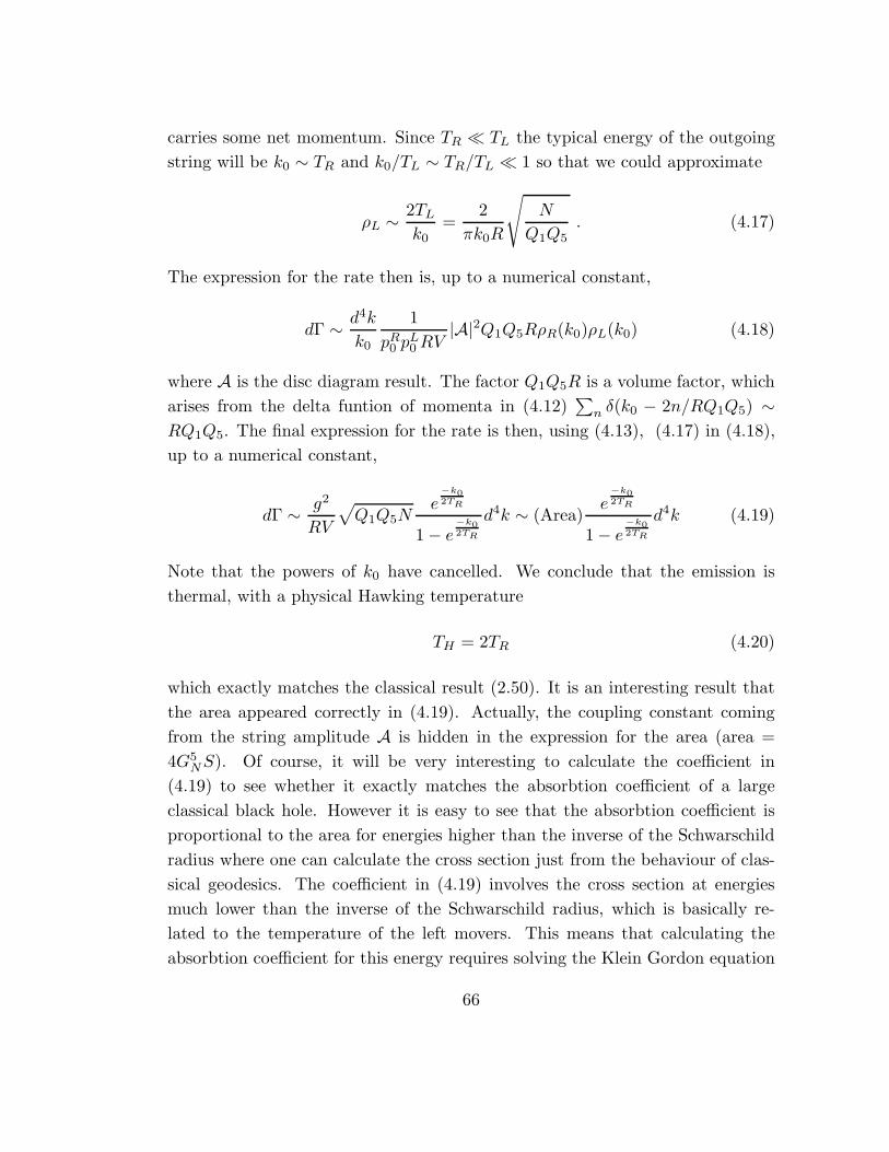
Waves

travel in

this direction

Compact dimensions

FIGURE 4: Ensemble of many oscillating strings carrying traveling waves.

In a very similar fashion it is possible to construct oscillating p-branes. In

fact, if we just average over the oscillations we simply get one more harmonic

function K = cP Nr7−p in the solution. The coefficient cP = α′

R29cf is calculated

using U-duality (see section 2.4) and N is the momentum, measured in units of

the minimum allowed. In conclusion, when momentum is carried in a direction

parallel to the brane (call it 9), then the solution can be found by replacing

−dt2 + dx29 → −dt2 + dx2

9 + k(dt − dx9)2 in the metric in (2.11) or (2.9) .

Adding momentum leads to BPS solutions preserving 1/4 of the supersymmetries

by imposing the additional constraints on the spinors at infinity, due to the

momentum,

ǫ0R = Γ0Γ9ǫ0R , ǫ0L = Γ0Γ9ǫ0L . (2.19)

2.3. d ≤ 9 Black Holes From d = 10 strings or branes.

Since all the BPS solutions treated in the previous section depend on

some harmonic function f one can make multiple brane solutions by taking

f = 1 +∑

i cp/(~r − ~ri)7−p which describes a set of branes at positions ~ri in

static equilibrium. The gravitational attraction is balanced by the repulsion due

to their charges.

In this section the word “brane” will indicate any of the BPS solutions

discussed above. We will now consider the type IIB theory compactified to d

dimensions on a torus T 10−d, identifying the coordinates by xi ∼ xi + 2πRi,

choosing periodic boundary conditions on this 10− d dimensional “box”. Fields

that vary over the box will acquire masses of the order m ∼ 1/R where R is

27

the typical compactification size. The easiest way to see this is by expanding

the fields in Fourier components along the internal dimensions. So if we are

interested in the low energy physics in d extended dimensions the fields will be

independent of the internal coordinates of the torus. If we want to find solutions

to this d dimensional supergravity theory, does it help us to know the solutions

in ten dimensions? Yes, it does. The key point to observe is that if we have any

solution in ten dimensions which is periodic under xi → xi + 2πRi, then it will

also be a solution of the compactified theory. For any p-brane, the solution is

automatically translational invariant in the directions parallel to the brane. In

order to produce a periodic solution we superimpose BPS solutions forming a

lattice in the transverse directions, producing a harmonic function

f = 1 +∑

~n∈Lattice

c

(~r − 2πRi~n)7−p. (2.20)

We can view this as solving the Laplace equation with the method of images in a

periodic box. It is this nice superposition principle for BPS solutions that enables

us to find a very direct correspondence between ten dimensional objects and the d

dimensional ones. We will be interested in solutions where the brane is completely

wrapped along the internal directions so that from the point of view of the

observer in d dimensions one has a localized, “spherically” symmetric solution.

These solutions will correspond to extremal limits of charged black hole solutions.

The first point to notice that if the brane wraps p of the torus dimensions then

the sum in (2.20) runs over a 10 − d − p dimensional lattice. If we are looking

at the solutions at distances much bigger than the compactification scale, then

we are allowed to replace the sum in (2.20) by an integral. This integral would

naturally appear also if we average over the position of the brane on the internal

torus. The net effect of the integral will be to give the function f = 1+c(d)P /rd−3,

where r is the distance in the extended d dimensional coordinates. Note that the

power of r is independent of p and is the appropriate one to be the spherically

symmetric solution to Laplace’s equation in d − 1 spatial dimensions. So when

we are in the d dimensional theory, the only way we have to tell that the black

hole contains a particular type of p brane is by looking at the gauge fields that

it excites. The final result is that the d dimensional solutions are given again by

(2.5), (2.9) and (2.11) but now in terms of d dimensional harmonic functions.

28

As a particular example we will consider the black holes resulting from com-

pactifying the oscillating strings treated in the previous section. The oscillation

will be along a compact direction, and we average over them. We could think

that we are looking at distances larger than the compactification radius, or that

we do an average over the phase of the oscillation. It is important that this

average is done at the level of the harmonic function that specifies the solu-

tion, and not on the individual components of the fields, which are non-linear in

terms of the harmonic functions. This procedure produces a solution of the d

dimensional supergravity theory. To be more precise, we build a periodic (9−d)dimensional array of strings by taking the harmonic function as in (2.20). For

large distances ρ in the extended dimensions we can ignore the dependence on

the internal dimensions and find,

f(d)f = 1 +

c(d)f m

ρd−3, where c

(d)f =

16πGdNR9

α′(d− 3)ωd−2, (2.21)

and ωd is the area of the d dimensional unit sphere and m is the total winding

number. We could have taken directly f(d)f as a solution of the Laplace equation

in the uncompactified dimensions, but we obtained it from superimposing solu-

tions to clarify the connection to underlying string states. As we will now show,

the result of this procedure can be interpreted as a lower-dimensional extremal

black hole. The general idea that ten-dimensional string solutions can be used

to generate four-dimensional black holes is not new and has been explored in

[46],[47],[48],[49],[42].

We now look in more detail at the d-dimensional fields generated by this

compactification. Using the dimensional reduction procedure of [50] , we find

that the d-dimensional fields obtained from wrapping a string with oscillations

are, in d-dimensional Einstein metric,

e−2φd =e−2φ10√

G99 =

√

f(d)f (1 + kd)

ds2E = − 1[

f(d)f (1 + kd)

]d−3d−2

dt2 +[

f(d)f (1 + kd)

]1

d−2

d~x2 .(2.22)

This and all the other fields obtained by dimensional reduction turn out to be the

type II analogs of Sen’s four-dimensional black holes and their higher-dimensional

29

generalizations [51], [52]. The Einstein metric of the d dimensional solution has

the same form if we consider any other oscillating brane completely wrapped

around the internal torus since the Einstein metric is invariant under U-duality.

We can check that for these black holes (2.22) the area of the horizon, which is

at ρ = 0, is zero, so that the classical entropy is zero. It is possible to define

a nonzero “classical” entropy at the “stretched” horizon which agrees up to a

numerical constant with the counting of states [53].

2.4. U-duality and quantization of the charges

We will show in this section how to quantize the charges using U-duality

[12]. There has been some disagreement in the literature concerning the precise

quantization condition so we have decided, for completeness, to explain it in

detail. Since the quantum of charge will depend on the normalization chosen for

the gauge field we find it more convenient to find the “quantum of mass”. This

quantity has a well defined meaning since the solution is BPS and the mass is

proportional to the charge and protected from quantum corrections so that it

can be calculated using the weakly coupled theory. When we perform S-duality

transformations we should remember that the mass measured in the Einstein

metric gE = e−φ/2G (which includes a power of g) stays invariant. This is not

how we normally measure masses, we normally leave a power of g in the Newton

constant. The masses we are going to calculate are defined in terms of a modified

Einstein metric which is gE = e−(φ−φ∞)

2 G = g1/2gE which agrees with the string

metric at infinity. All we are saying is that we keep the factor of g2 in the Newton

constant. Masses measured in the two metrics differ by ME = g1/4M , where M

is the mass measured in the metric gE which is the one we are going to use

here. The d dimensional Newton constant is GdN = G10

N /V10−d where V10−d is

the volume of the internal torus. We start with the minimum mass of a winding

string which is (1.2)

Mf =R9

α′ . (2.23)

Similarly the minimum mass for momentum states is M = 1/R. Now we want

to calculate the mass of a D-string with unit winding using ten dimensional S-

duality. We know that the Einstein metric is invariant under S-duality so that

ME is invariant, this implies

g′1/4M ′ = M ′E = ME = g1/4R9

α′ (2.24)

30

so that the mass of the D-string is

M1D =R9

gα′ , (2.25)

where we took into account the change in R9 as in (1.7). Applying T-duality

transformations (1.5) along a direction perpendicular to the D-string we turn it

into a D-twobrane with mass

M =R9

gα′ =R9R

′8

g′α′3/2. (2.26)

Proceeding in this fashion we find the minimum mass for any D-brane

MpD =R10−p · · ·R9

gα′(p+1)/2. (2.27)

Doing now an S-duality transformation on the D-fivebrane, as in (2.24) we get

the mass of the solitonic fivebrane

M s5 =R5 · · ·R9

g2α′3 . (2.28)

Our objective is to determine the coefficients that appear in the harmonic func-

tions specifying the solutions (2.5)(2.9)(2.11). Since we will be mainly interested

in four and five dimensional black holes we are interested in the coefficient that

appears in the d dimensional harmonic functions as in (2.21)(2.22). Actually

from (2.22) by setting k(d) = 0 we can read off the mass of these objects in terms

of the coefficients in the harmonic function f (d). The mass is calculated from the

behaviour of gE 00 of the metric at infinity [54]

gE 00 ∼ 16πGdNM

(d− 2)ωd−2

1

rd−3=d− 3

d− 2

c(d)

rd−3(2.29)

where ωn is the volume of the unit sphere Sn, ωn = 2πn/2

Γ(n/2) . This determines the

coefficients for all excitations. We still have to express GN in terms of g, remem-

ber that we defined g to be such that it goes to 1/g under S-duality (1.7). In

order to do that, we use Dirac duality of the fundamental string and the solitonic

fivebrane. The fundamental string carries electric charge under the NSNS Bµν

field while the solitonic fivebrane carries magnetic charge. It is not possible to

31

define globally the Bµν field of the fivebrane (2.9). This field will contain a sin-

gularity, analogous to the Dirac string for a monopole in electrodynamics. The

condition that this singularity is invisible for the fundamental strings fixes the

coefficient of the fivebrane harmonic function as c(5)s5 = α′ [40]4. Comparing this

value with the one resulting from (2.29) and (2.28) we find the ten dimensional

Newton constant

G10N = 8π6g2α′4 . (2.30)

In string theory one can independently calculate the mass of D-branes from

virtual closed string exchange diagrams, in a similar fashion as one calculates the

force between two charges in quantum electrodynamics. The string “miracle” [8]

is that this string theory calculation of masses of D-branes agrees with the masses

predicted by U-duality as above.

Now for later convenience let us quote the results, which are obtained from

(2.27)(2.29)(2.30) for the D-onebrane, D-fivebranes and momentum in five ex-

tended dimensions, which we will need for the five dimensional black holes,

c(5)1 =

4G5NR9

πα′g, c

(5)5 = gα′ , c

(5)P =

4G5N

πR9. (2.31)

We will also need the corresponding coefficients for D-twobranes, D-

sixbranes, solitonic fivebranes and momentum in four extended dimensions

c(4)2 =

4G4NR4R9

gα′3/2, c

(4)5 =

α′

2R4,

c(4)6 =

gα′1/2

2, c

(4)P =

4G4N

R9,

(2.32)

where we have used the value of the Newton constant (2.30).

4 Note that in comparing with [40] we only have to check that they used the same

definition of the string tension as in (1.1).

32

2.5. Black hole solutions in five dimensions.

In section 2.3 we considered black holes coming from wrapping just one type

of branes on the torus, or at most one type of branes with oscillations. All those

black holes have zero horizon area and are singular at the horizon, since there

are scalar fields diverging at the horizon. By looking at the classical solutions

we see that in almost all of them the dilaton is going to plus or minus infinity.

Also the physical longitudinal size goes to zero, measured in Einstein metric, for

all the branes with no oscillations. Adding momentum in the internal directions

does not help, we still have some diverging scalar. The three brane (2.11) has

constant dilaton but suffers of this problem about the physical size.

Our goal is to construct solutions with well defined geometries at the horizon,

like the ones appearing in General Relativity. The key principle is that we need to

balance the scalars at the horizon. Different branes have different scalar charges,

which can be interpreted as pressures or tensions in the compact direction. Note

that even the dilaton falls in this category when we think of it as the size of the

11th dimension in M-theory. If a scalar diverges when we approach the horizon

the d dimensional character of the solution is lost. This forces us to consider

more than one type of branes. We need three different types for black holes

in five dimensions and four different types for black holes in d = 4, here two

non-parallel p-branes count as being of different type.

2.5.1. Extremal black holes in five dimensions.

We construct the five dimensional black hole with nonzero area by superpos-

ing a number Q5 of D-fivebranes, Q1 D-onebranes and Kaluza-Klein momentum.

We consider type IIB compactified on T 5. We wrap a number Q5 of D-fivebranes

on T 5. Then we wrap Q1 D-strings along one of the directions of the torus, let us

pick the 9th direction. In addition we put some momentum P9 = N/R9 along the

string, i.e. in the direction 9. The solution is given by three harmonic functions

f5, f1 and k. We start writing the solution in terms of the ten dimensional string

33

metric, so that the relation to (2.11) becomes more apparent [55][14]

ds2str =f− 1

21 f

− 12

5

(

−dt2 + dx29 + k(dt− dx9)

2)

+

+f121 f

125 (dx2

1 + · · · + dx24) + f

121 f

− 12

5 (dx25 + · · ·+ dx2

8) ,

e−2(φ10−φ∞) =f5 f−11 ,

B′09 =

1

2(f−1

1 − 1) ,

H ′ijk =(dB′)ijk =

1

2ǫijkl∂lf5 , i, j, k, l = 1, 2, 3, 4

(2.33)

where ǫijkl is again the flat space epsilon tensor. The three harmonic functions

are

f1 = 1 +c(5)1 Q1

x2, f5 = 1 +

c(5)5 Q5

x2, k =

c(5)P N

x2(2.34)

with x2 = x21+· · ·+x2

4 and the coefficients are given in (2.31). The components of

the Ramond-Ramond antisymmetric tensor field, B′RRµν , that are excited behave

as gauge fields when we dimensionally reduce to five dimensions. The three

independent charges arise as follows: Q1 is a RR electric charge, coming from

B′RR09 and counts the 1D-branes. Q5 is a magnetic charge for the three form

field strength H ′RR3 = dB′RR

2 , which is dual in five dimensions to a gauge field,

F2 = ∗5H′RR3 . Q5 is thus an electric charge for the gauge field F2 and it counts the

number of 5D-branes. The third charge, N , corresponds to the total momentum

along the branes in the direction 9, and it is associated to the five dimensional

Kaluza-Klein gauge field coming from the G09 component of the metric.

Let us understand what happens to the supersymmetries. In the ten dimen-

sional type IIB theory the supersymmetries are generated by two independent

chiral spinors ǫR and ǫL ( Γ11ǫR,L = ǫR,L). The presence of the D-strings and the

D-fivebranes imposes additional conditions on the surviving supersymmetries

ǫR = Γ0Γ9ǫL , ǫR = Γ0Γ5Γ6Γ7Γ8Γ9ǫL , (2.35)

where the first condition is due to the presence of the string and the second to the

presence of the fivebrane (1.16). When we put momentum we break additional

supersymmetries through the conditions

Γ0Γ9ǫR = ǫR , Γ0Γ9ǫL = ǫL. (2.36)

34

Taken together with (2.35) we get the following decomposition of the spinor

under the group S0(1,1)×SO(4)E×SO(4)I , which is the subgroup of Lorentz

transformations that leaves the ten dimensional solution (2.33) invariant,

ǫL = ǫR = ǫ+SO(1,1)ǫ+SO(4)ǫ

+SO(4) . (2.37)

The positive chirality SO(4) spinor is pseudoreal and has two independent com-

ponents so that 1/8 (4 out of the original 32) supersymmetries are preserved

by this configuration. The first SO(4)E corresponds to spatial rotations in 4+1

dimensions. SO(4)I corresponds to rotations in the internal directions 5, 6, 7, 8

and is broken by the compactification. The solution is supersymmetric, and has

the same energy, independent on whether all the branes are sitting at the same

point or not, so in principle we can separate the different constituents of the black

hole. The resulting black hole will have lower entropy so this process violates the

second law of thermodynamics.

Now we dimensionally reduce (2.33) to five dimensions in order to read off

black hole properties. The standard method of [56] yields a five-dimensional

Einstein metric, g5E = e−4φ5/3G5

string,

ds2E = − 1

(f1f5(1 + k))23

dt2 + (f1f5(1 + k))13 (dx2

1 + · · ·+ dx24) , (2.38)

which describes a five dimensional extremal, charged, supersymmetric black hole

with nonzero horizon area. Calculating the horizon area in this metric (2.38) we

get the entropy

Se =AH

4G5N

= 2π√

NQ1Q5 . (2.39)

In this form the entropy does not depend on any of the continuous parameters like

the coupling constant or the sizes of the internal circles, etc. This “topological”

character of the entropy was emphasized in [57], [58], [55]. It is also symmetric

under interchange of N,Q1, Q5. In fact, U duality [12], [59], [60] interchanges the

three charges. To show it in a more specific fashion, let us define Ti to be the

usual T-duality that inverts the compactification radius in the direction i and S

the ten dimensional S duality of type IIB theory. Then a transformation that

sends (N,Q1, Q5) to (Q1, Q5, N) is U= T8T7T6T5ST6T9. Note however that

this transformation changes the coupling constant and the sizes of the T 5.

35

The standard five-dimensional extremal Reissner-Nordstrom solution [54] is

recovered when the charges are chosen such that

cPN = c1Q1 = c5Q5 = r2e . (2.40)

The crucial point is that, for this ratio of charges, the dilaton field and the in-

ternal compactification geometry are independent of position and the distinction

between the ten-dimensional and five-dimensional geometries evaporates. What

is at issue is not so much the charges as the different types of energy-momentum

densities with which they are associated. An intuitive picture of what goes on

is this [14]: a p-brane produces a dilaton field of the form e−2φ10 = fp−32

p , with

fp a harmonic function [28]. A superposition of branes produces a product of

such functions and one sees how 1-branes can cancel 5-branes in their effect on

the dilaton. A similar thing is true for the compactification volume: For any

p-brane, the string metric is such that as we get closer to the brane the volume

parallel to the brane shrinks, due to the brane tension, and the volume perpen-

dicular to it expands, due to the pressure of the electric field lines. It is easy to

see how superposing 1-branes and 5-branes can stabilize the volume in the di-

rections 6, 7, 8, 9, since they are perpendicular to the 1-brane and parallel to the

5-brane. The volume in the direction 5 would still seem to shrink, due to the ten-

sion of the branes. This is indeed why we put momentum along the 1-branes, to

balance the tension and produce a stable radius in the 5 direction. If we balance

the charges precisely (2.40) (we can always do this for large charges) the moduli

scalar fields associated with the compactified dimensions are not excited at all,

which is what we need to get the Reissner-Nordstrom black hole. Of course, if

we do not balance them precisely we still have a black hole with nonzero area,

as long as the three charges are nonzero.

2.5.2 Non-extremal black holes in five dimensions.

The five dimensional Reissner-Nordstrom black hole is a solution of the five

dimensional Einstein plus Maxwell action. The metric reads [54]

ds2 = −λdt2 + λ−1dr2 + r2dΩ23 , (2.41)

λ =

(

1 − r2+r2

)(

1 − r2−r2

)

.

36

There is a horizon at r = r+, mass and charge are given by

M =3π

8G5N

(r2+ + r2−) , Q =3π

4G5N

r+r− . (2.42)

The extremal solution is obtained by taking r+ = r− ≡ re and reduces to (2.38),

with the charges related by (2.40), after doing the coordinate transformation

r2 = x2 + r2e .

Now we would like to construct the non-extremal five dimensional black

holes with arbitrary values of the charges. The method is very simple [18][17].

First we start with the non-extremal Reissner-Nordstrom (2.41) which has some

constraints on the charges (2.40), then we lift up this configuration to ten dimen-

sions. That is done by inverting the standard dimensional reduction procedure

[56], and we find the ten dimensional form of the various fields. This gives a

non-extremal configuration where the charges are related by (2.40). We will

apply some transformations which remove the constraints of (2.40). We start

by boosting the solution along the direction of the onebranes (we called it 9).

This introduces some extra momentum, so that now the RR charges are con-

strained but the momentum is arbitrary. The result is a solution which can be

viewed as a black string in six dimensions [18]. Now we need to remove the

constraint on the RR charges. To that effect we do a U duality transforma-

tion that interchanges the three different charges. More precisely we perform the

transformation U=T8T7T6T5ST6T9 that sends (N,Q1, Q5) to (Q1, Q5, N). This

transformed one RR charge into momentum, so that we can boost the solution

to produce a solution with arbitrary value of this RR charge. After doing all

these transformations, and choosing some appropriate coordinates, the resulting

ten dimensional solution is, in string metric,

e−2(φ−φ∞) =

(

1 +r20sinh2γ

r2

) (

1 +r20sinh2α

r2

)−1

, (2.43)

ds2str =

(

1 +r20sinh2α

r2

)−1/2 (

1 +r20sinh2γ

r2

)−1/2[

−dt2 + dx29

+r20r2

(coshσdt+ sinhσdx9)2 +

(

1 +r20sinh2α

r2

)

(dx25 + . . .+ dx2

8)

]

+

(

1 +r20sinh2α

r2

)1/2 (

1 +r20sinh2γ

r2

)1/2[

(

1 − r20r2

)−1

dr2 + r2dΩ23

]

.

(2.44)

37

This solution is parameterized by the six independent quantities α, γ, σ, r0, R9 ≡R and V . The last two parameters are the radius of the 9th dimension and the

product of the radii in the other four compact directions V = R5R6R7R8. They

appear in the charge quantization conditions, indeed the three charges are

Q1 =V

4π2g

∫

eφ6 ∗H ′ =V r202g

sinh 2α,

Q5 =1

4π2g

∫

H ′ =r202g

sinh 2γ,

N =R2V r20

2g2sinh 2σ,

(2.45)

where ∗ is the Hodge dual in the six dimensions x0, .., x5. For simplicity we set

from now on α′ = 1. The last charge N is related to the momentum around the

S1 by P9 = N/R9. All charges are normalized to be integers.

Reducing (2.44) to five dimensions using [56], the solution takes the remark-

ably simple and symmetric form:

ds25 = −λ−2/3

(

1 − r20r2

)

dt2 + λ1/3

[

(

1 − r20r2

)−1

dr2 + r2dΩ23

]

, (2.46)

where

λ =

(

1 +r20sinh2α

r2

) (

1 +r20sinh2γ

r2

) (

1 +r20sinh2σ

r2

)

. (2.47)

This is just the five-dimensional Schwarzschild metric with the time and space

components rescaled by different powers of λ. The factored form of λ was known

to hold for extremal solutions (2.38) [49]. It is surprising that it continues to

hold even in the non-extremal case. The solution is manifestly invariant under

permutations of the three boost parameters as required by U-duality. The event

horizon is clearly at r = r0. The coordinates we have used present the solution in

a simple and symmetric form, but they do not always cover the entire spacetime.

When all three charges are nonzero, the surface r = 0 is a smooth inner horizon.

This is analogous to the situation in four dimensions with four charges [61].

When at least one of the charges is zero, the surface r = 0 becomes singular.

Several thermodynamic quantities can be associated to this solution. They can

38

be computed in either the ten dimensional or five dimensional metrics and yield

the same answer. For example, the ADM energy is

E =RV r202g2

(cosh 2α+ cosh 2γ + cosh 2σ) . (2.48)

The Bekenstein-Hawking entropy is

S =A10

4G10N

=A5

4G5N

=2πRV r30

g2coshα cosh γ coshσ. (2.49)

where A is the area of the horizon and we have used the value (2.30) for the

Newton constant. The Hawking temperature is

T =1

2πr0 coshα cosh γ cosh σ. (2.50)

In ten dimensions, the black hole is characterized by pressures which describe how

the energy changes for isentropic variations in R and V . In five dimensions, these

are ‘charges’ associated with the two scalar fields coming from the components

G99 and G55 in (2.44), which can be interpreted as the pressures in the directions

9 and 5 respectively, and they read

P1 =RV r202g2

[

cosh 2σ − 1

2(cosh 2α+ cosh 2γ)

]

,

P2 =RV r202g2

(cosh 2α− cosh 2γ) .

(2.51)

The extremal limit corresponds to the limit r0 → 0 with at least one of the

boost parameters α, γ, σ → ±∞ keeping R, V and the associated charges (2.45)

fixed. If we keep all three charges nonzero in this limit, one obtains

Eext =R|Q1|g

+RV |Q5|

g+

|N |R

,

Sext = 2π√

|Q1Q5N | ,Text = 0 ,

P1ext =|N |R

− R|Q1|2g

− RV |Q5|2g

,

P2ext =R|Q1|g

− RV |Q5|g

.

(2.52)

39

The first equation is the saturated Bogomolnyi bound for this theory.

We now show that there is a formal sense in which the entire family of

solutions discussed above can be viewed as “built up” of branes, anti-branes, and

momentum. The extremal limits with only one type of excitation are obtained

by letting r0 go to zero and taking a boost parameter go to infinity keeping only

one charge fixed. These extremal metrics represent a D-onebrane wrapping the

S1, or a D-fivebrane wrapping the T 5, or the momentum modes around the S1.

From (2.48) and (2.51) we see that a single onebrane or anti-onebrane has mass

and pressures

M =R

g, P1 = − R

2g, P2 =

R

g. (2.53)

Of course a onebrane has Q1 = 1, while an anti-onebrane has Q1 = −1. A single

fivebrane or anti-fivebrane has

M =RV

g, P1 = −RV

2g, P2 = −RV

g. (2.54)

For left- or right-moving momentum

M =1

R, P1 =

1

R, P2 = 0 (2.55)

Given (2.53) - (2.55), and the relations (2.45), (2.48), and (2.51), it is

possible to trade the six parameters of the general solution for the six quan-

tities (N1, N1, N5, N5, NR, NL) which are the “numbers” of onebranes,

anti-onebranes, fivebranes, anti-fivebranes, right-moving momentum and left-

moving momentum respectively. This is accomplished by equating the total

mass, pressures and charges of the black hole with those of a collection of

(N1, N1, N5, N5, NR, NL) non-interacting “constituent” branes, antibranes

and momentum. By non-interacting we mean that the masses and pressures are

simply the sums of the masses and pressures of the constituents. The resulting

40

expression for the N ’s are

N1 =V r204g

e2α,

N1 =V r204g

e−2α ,

N5 =r204ge2γ ,

N5 =r204ge−2γ ,

NR =r20R

2V

4g2e2σ,

NL =r20R

2V

4g2e−2σ.

(2.56)

(2.56) is the definition of the N ’s, but we will refer to them as the numbers of

branes, antibranes and momentum because (as will be seen) they reduce to those

numbers in certain limits where these concepts are well defined.

In terms of the numbers (2.56), the charges are simply Q1 = N1−N1, Q5 =

N5 −N5, N = NR −NL, the total energy is

E =R

g(N1 +N1) +

RV

g(N5 +N5) +

1

R(NR +NL) , (2.57)

and the volume and radius are

V =

(

N1N1

N5N5

)1/2

, (2.58)

R =

(

g2NRNL

N1N1

)1/4

. (2.59)

From (2.52) we see that the extremal solutions correspond to including either

branes or anti-branes, but not both. Notice that for the general Reissner-

Nordstrom solutions (α = γ = σ) the contribution to the total energy from

onebranes, fivebranes, and momentum are all equal:

R

g(N1 +N1) =

RV

g(N5 +N5) =

1

R(NR +NL). (2.60)

41

The actual number of branes of each type depends on R and V and can be very

different.

Of course there seems to be no reason for neglecting interactions between

collections of branes and momentum modes composing a highly non-extremal

black hole at strong or intermediate coupling. Hence the definitions (2.56) would

seem to be inappropriate for describing a generic black hole. However, the utility

of these definitions can be seen when we reexpress the black hole entropy (2.49)

in terms of the N ’s. It takes the remarkably simple form

S = 2π(√

N1 +√

N1)(√

N5 +√

N5)(√

NL +√

NR) . (2.61)

In the next chapter we will compute this formula in string theory in some special

limits. An interesting property of this entropy formula (2.61) is that if one takes

the brane-antibrane numbers to be free variables and then one maximases the

entropy (2.61) subject to the constraints that the charges and the total energy

(2.57) are fixed, then one gets the relations (2.59)(2.58) and hence (2.56) for the

brane-antibrane numbers. So, in this very specific sense, the black hole solution

represents a system of branes and antibranes in thermodynamic equilibrium.

A puzzling feature of (2.61) is that it only involves onebranes, fivebranes, and

momentum. This is understandable for extremal solutions with these charges,

but when one moves away from extremality, one might expect pairs of threebranes

and anti-threebranes or fundamental string winding modes to contribute to the

entropy. To understand the roles of these other objects, one should start with

the full Type II string theory compactified on T 5. The low energy limit of this

theory is N = 8 supergravity in five dimensions (we measure N in four d terms,

i.e. by the amount of supersymmetry that it has reduced to d = 4). This theory

has 27 gauge fields, 42 scalars and a global E6 symmetry. Since only the scalar

fields which couple to the gauge fields are nontrivial in a black hole background,

we expect the general solution to be characterized by 27 scalars in addition to

the 27 charges. One can interpret the 27 scalar parameters as 26 scalars plus

the ADM energy. Each charge corresponds to a type of soliton or string. Thus

we expect the solution to again be characterized by the number of solitons and

anti-solitons. For an extremal black hole, the entropy can be written in the E6

invariant form [62], [63]

S = 2π|TABCVAV BV C |1/2 , (2.62)

42

where V A is the 27 dimensional charge vector and TABC is a symmetric cubic

invariant in E6. For the non-extremal black holes, the above argument suggests

that one can introduce two vectors V Ai i = 1, 2 which represent the number of

solitons and anti-solitons. Although we have not done the calculation, the general

black hole entropy might take the E6 invariant form

S = 2π∑

i,j,k

|TABCVAi V B

j V Ck |1/2 , (2.63)

where i, j, k = 1, 2, V A1 indicates the number of charges and V A

2 the number of

anticharges, each is a vector in the 27 of E6. The entropy of non-extremal black

holes can be represented in terms of charges and anti-charges in many different

(equivalent) ways which are related by E6 transformations. Now we see that our

choice of D-onebranes, D-fivebranes and momentum was like a choice of basis

and other configurations are related by E6(Z) U-duality transformations.

One can similarly construct rotating black holes in five dimensions. The

spatial rotation group is SO(4)E ∼ SU(2)R×SU(2)L. We we can view the an-

gular momentum as a 4×4 antisymmetric matrix. We can choose a basis such

that it reduces to 2×2 blocks, each block corresponds to a rotation on a plane

and there are two orthogonal planes. The angular momentum is characterized

by the angular momentum eigenvalues J1, J2 on these two planes. Also the an-

gular momenta are characterized by the U(1) charges FR/2, FL/2 which are two

eigenvalues of the SU(2)’s (we define FR,L to have integer eigenvalues). We have

J1 =1

2(FR + FL), J2 =

1

2(FR − FL) . (2.64)

The solution with angular momentum can be found in [15], [16], [64], we will be

just interested in the entropy of that solution in the extremal limit, for which the

mass is the minimum consistent with a given angular momentum and charges.

The entropy is then

Sext = 2π√

NQ1Q5 − J1J2 . (2.65)

For J1 = J2 the solution is also BPS [15].

43

2.6. Black hole solutions in four dimensions

Now we turn to the more realistic case of four dimensional black holes. It

is still not totally realistic since the compactification we will consider is on T 6

which is not the one that describes our four dimensional world. The supergravity

theory however contains black hole solutions which are exactly those of General

Relativity. The difference between the two theories is that the N=8 supergravity

theory one obtains by compactifying on T 6 has many more gauge fields (28 of

them) and massless scalars (70 of them). Black hole solutions are characterized

by 56 charges, 28 electric and 28 magnetic. One hopes that the general features

of black hole physics will not depend too much on the content of the theory, as

long as it includes gravity and one is studying black holes with the same metric

as the ones appearing in General Relativity. In fact some of the solutions we

study are also solutions in general relativity.

2.6.1 Extremal black holes in four dimensions

Let us start with the extremal black holes [19], [20]. Taking the configura-

tion of 1D-branes, 5D-branes and momentum that we had in d = 5 and putting it

on T 6 we obtain a black hole solution that preserves 1/8 of the supersymmetries.

In order to put it on T 6 one has to form a lattice of the extremal five dimensional

black holes (2.33) and define new harmonic functions as in (2.20). This makes

all harmonic functions to depend on 1/r where now r is the spatial distance in

1+3 dimensions. The unbroken supersymmetries are given by (2.37). Now we do

a T duality transformation (along the direction 4) to the IIA theory and we get

a system of 2D-branes, 6D-branes and momentum. In addition we flip the chi-

rality of the ten dimensional spinor ǫR. We will have ǫIIAR = Γ4ǫIIB

R , so that the

chirality that is flipped in ǫR is that of the “external” SO(4)E . Of course, only

the SO(3) subgroup corresponding to spatial rotations in the directions 1, 2, 3 is

a symmetry of the solution. However, this black hole has zero area and has a

singular geometry at the horizon. The reason is that some of the scalar fields are

unbalanced, for example, we can see from (2.11) that the dilaton field will not

go to a constant as we approach the horizon, e−2φ = f−1/22 f

3/26 . It is interesting

that one can put an additional type of charge without breaking any additional

supersymmetry. This charge has to be a solitonic fivebrane, it is the only one al-

lowed by supersymmetry that is not just a U-duality tranformation of the others.

44

This, in a sense, is analogous to putting left moving oscillations on a macroscopic

heterotic string [42] which does not break any additional supersymmetry. It also

has the virtue of balancing all the scalars, for example the dilaton now behaves

as e−2φ = f−1/22 f

3/26 f−1

s5 . In order to be more precise let us say that our torus is

T 6 = T 4 × S′1 × S1 and we have the 6D-branes wrapping all T 6, the 2D-branes

wrap S′1 × S1 (directions 4, 9), the solitonic fivebranes wrap T 4 × S1 (directions

5, 6, 7, 8, 9) and the momentum is flowing along S1 (direction 9). Notice that the

momentum flows parallel to the fivebranes and the two D-branes.

We can see from (1.16),(2.19) and (2.10) that the fivebrane does not break

any additional supersymmetry. The final configuration still preserves 1/8 of

the original supersymmetries. Decomposing the surviving spinor in terms of

SO(1,1)×SO(4)E×SO(4)I we find

Γ4ǫR = ǫL = ǫ+SO(1,1)ǫ+SO(4)ǫ

+SO(4) . (2.66)

The extremal four dimensional black hole, constructed this way, written in

ten dimensional string metric, has the form [55]

ds2str =f− 1

22 f

− 12

6

(

−dt2 + dx29 + k(dt− dx9)

2)

+ fs5f− 1

22 f

− 12

6 dx24+

+f122 f

− 12

6 (dx25 + · · · + dx2

8) + fs5f122 f

126 (dx2

1 + · · ·+ dx23) ,

e−2(φ10−φ∞) =f−1s5 f

− 12

2 f326 ,

Hij4 =1

2ǫijk∂kfs5 i, j, k = 1, 2, 3 ,

C049 =1

2(f−1

2 − 1) ,

(dA)ij =1

2ǫijk∂kf6 i, j, k = 1, 2, 3 ,

(2.67)

where ǫijk is the flat space epsilon tensor. The harmonic functions are

f2 = 1+c(4)2 Q2

r, f5 = 1+

c(4)s5 Q5

r, f6 = 1+

c(4)6 Q6

r, k =

c(4)P N

r, (2.68)

where the coefficients c(4)’s are given in (2.32) and the charges Q2, Q5, Q6, N are

integers. Calculating the entropy we find

S =A4

4G4N

= 2π√

Q2Q5Q6N , (2.69)

45

which is, as (2.39), U-dual and independent of the moduli.

2.6.2 Non-extremal black holes in four dimensions

In a similar way as we did for five dimensions one can construct the non-

extremal four dimensional solution. After doing the dimensional reduction to

four dimensions the Einstein metric reads [61]5

ds2 = −χ−1/2(r)(

1 − r0r

)

dt2 + χ1/2(r)

[

(

1 − r0r

)−1

dr2 + r2(dθ2 + sin2 θdφ2)

]

,

χ(r) =

(

1 +r0 sinh2 α2

r

) (

1 +r0 sinh2 α5

r

) (

1 +r0 sinh2 α6

r

) (

1 +r0 sinh2 αp

r

)

.

(2.70)

This metric is parameterized by the five independent quantities α2, α5, α6, αp

and r0. The event horizon lies at r = r0. The special case α2 = α5 = α6 = αp

corresponds to the Reissner-Nordstrom metric (2.1), so that we see that, as we

promised, the General Relativity solution is among the cases studied. The overall

solution contains three additional parameters which are related to the asymptotic

values of the three scalars. From the ten-dimensional viewpoint, these are the

product of the radii of T 4, V = R5R6R7R8, and the radii of S1 and S′1, R9

and R4, and they appear in the quantization condition for the charges. There

are, in addition, U(1) gauge fields excited, corresponding to the four physical

charges. One is the Kaluza Klein gauge field coming from the component G09

of the metric, which carries the momentum charge, N . Then we have a RR

gauge field coming from the component C049 of the three form RR potential

which carries the 2D-brane charge, Q2. The 6D brane charge, Q6, appears as

magnetic charge for the one form RR potential Aµ, and finally the fivebrane

charge, Q5 also appears as magnetic charge for the gauge field coming from the

NS antisymmetric tensor with one index along the direction 4, Bµ4.

5 We use the classical solution from [61] but with our quantization condition for

the charges derived in section (2.4).

46

The physical charges are expressed in terms of these quantities as [21]

Q2 =r0V

gsinh 2α2 ,

Q5 = r0R4 sinh 2α5 ,

Q6 =r0g

sinh 2α6 ,

N =r0V R

29R4

g2sinh 2αp ,

(2.71)

where we have again set α′ = 1 and from (2.30) the four-dimensional Newton

constant becomes G4N = g2/(8V R4R9).

The ADM mass of the solution is

M =r0V R4R9

g2(cosh 2α2 + cosh 2α5 + cosh 2α6 + cosh 2αp) (2.72)

and the Bekenstein-Hawking entropy is

S =A4

4G4N

=8πr20V R4R9

g2coshα2 coshα5 coshα6 coshαp . (2.73)

There are three nontrivial scalar fields present in the solution and associated

with these scalar fields are three pressures (scalar charges)

P1 =r0V R4R9

g2(cosh 2α2 + cosh 2α6 − cosh 2α5 − cosh 2αp) ,

P2 =r0V R4R9

g2(cosh 2α2 − cosh 2α6) ,

P3 =r0V R4R9

g2(cosh 2α5 − cosh 2αp) .

(2.74)

As we did for the five dimensional black hole in section (2.5) we calculate the

values for the mass and scalar charges of each type of brane or string. This can be

calculated from the solution we have presented by taking the four extremal limits:

r0 → 0, αi → ±∞ with Qi and αj (j 6= i) fixed. We find that D-twobranes have

mass and pressures [21]

M = P1 = P2 =R4R9

g, P3 = 0 , (2.75)

47

while for the D-sixbranes we have

M = P1 = −P2 =V R4R9

g, P3 = 0 . (2.76)

For the solitonic fivebrane we have

M = −P1 = P3 =V R9

g2, P2 = 0 , (2.77)

and for the momentum we find

M = −P1 = −P3 =1

R9, P2 = 0 . (2.78)

Using these relations plus the charges (2.71) we trade in the eight parameters

of the solution for the eight quantities (NR, NL, N2, N2, N5, N5, N6, N6) which are

the numbers of right(left)-moving momentum modes, twobranes, anti-twobranes,

fivebranes, anti-fivebranes, sixbranes and anti-sixbranes. We do this by match-

ing the mass (2.72), pressures (2.74), and gauge charges (2.71) with those of a

collection of noninteracting branes. This leads to

NR =r0V R

29R4

2g2e2αp ,

N2 =r0V

2ge2α2 ,

N5 =r0R4

2e2α5 ,

N6 =r02ge2α6 ,

NL =r0V R

29R4

2g2e−2αp ,

N2 =r0V

2ge−2α2 ,

N5 =r0R4

2e−2α5 ,

N6 =r02ge−2α6 .

(2.79)

In terms of the brane numbers, the ADM mass is reexpressed as

M =1

R1(NR +NL) +

R9R4

g(N2 +N2) +

V R9

g2(N5 +N5) +

V R9R4

g(N6 +N6) ,

(2.80)

the gauge charges are simply differences of the brane numbers, and the other

parameters are

V =

√

N2N2

N6N6

, R4 =

√

N5N5

g2N6N6

, R29R4 =

√

g2NRNL

N2N2

. (2.81)

48

The entropy (2.73) then takes the surprisingly simple form

S = 2π(√

NR +√

NL)(√

N2 +√

N2)(√

N5 +√

N5)(√

N6 +√

N6) . (2.82)

This is the analog of (2.61) for four-dimensional black holes. When one term

in each factor vanishes, the black hole is extremal (2.69). Although we cannot

derive the general formula from counting string states, we will do so in certain

limits corresponding to near-extremal black holes.

Since the full theory should be E7 invariant we should be able to write

the general entropy formula in an invariant way. If we denote by V A1 the 56-

dimensional vector giving the number of solitons and by V A2 the number of anti-

solitons, the formula for the entropy takes the form [65][66]

S = 2π∑

i,j,k,l

√

TABCDVAi V B

j V Ck V D

l , (2.83)

where TABCD is the E7 quartic invariant.

We now consider adding rotation to the black holes discussed above. Since

the rotation dependent terms in the solution fall off faster at infinity than the

charges, the definition of the brane numbers (2.79) is unchanged. If we take nearly

extremal black holes with N2 ∼ N5 ∼ N6 ∼ 0, and R1 large, the Bekenstein-

Hawking entropy takes the form [64]

S = 2π(

√

NRN2N5N6 +√

NLN2N5N6 − J2)

. (2.84)

where J is the angular momentum of the black hole.

49

3. D-BRANE DESCRIPTION OF BLACK HOLES

In this chapter we will describe some properties of the black holes that we

studied in chap. 2 in terms of the D-brane string solitons described in chap. 1.

The black holes we study have non-zero horizon area and contain, as special cases,

the charged black holes of general relativity. The description that will emerge

depends on some detailed properties of the string theory D-brane solitons which

are obvious from just the supergravity theory. The key property that will be

used is that when many D-branes sit at the same point there is a large number of

massless states coming from open strings with ends attached to different branes

[9].

We will start with the five dimensional black hole which is simpler because it

involves only three different kinds of charge. Then we treat the four dimensional

case. In both cases we will start with the BPS extremal black holes where the

calculation of the entropy can be justified on the basis of supersymmetry and

then we will explore the near-extremal limits.

4. Extremal Five dimensional black holes.

We consider the type IIB theory on T 5 = T 4 × S1. We consider a config-

uration of Q5 D-fivebranes wrapping the whole T 5, Q1 D-strings wrapping the

S1 and momentum N/R9 along the S1, choosing this S1 to be in the direction

9. All charges N,Q1, Q5 are integers (2.38).

Since extremal D-branes are boost invariant along the directions parallel to

the branes they cannot carry momentum along S1 by just moving rigidly. Our

first task will be to identify the D-brane excitations that carry the momentum. In

the discussion of the oscillating fundamental string in sec. (2.2) the momentum

was carried by the oscillations. However, just oscillations of the branes do not

have enough entropy to match the classical result. As we saw in the D-brane sec-

tion, oscillations of the branes are described by massless open strings with both

ends attached to the same brane. There are many types of open strings to con-

sider: those that go from one 1-brane to another 1-brane, which we denote as (1,1)

strings, as well as the corresponding (5,5), (1,5) and (5,1) strings (the last two

being different because the strings are oriented). We want to excite these strings

50

and put some momentum on them. As it was shown for oscillating D-branes in

section 1.3 exciting some of them makes others massive so we have to see what is

the way to excite the stings so that a maximum number remains massless, since

this configuration will have the highest entropy. Let us work out the properties

of (1,5) and (5,1) strings. The string is described by the action (1.1) where two

of the coordinates have Neumann-Neumann boundary conditions (X0, X9), four

coordinates have Dirichlet-Dirichlet boundary conditions (X1, X2, X3, X4) and

the other four have Neumann-Dirichlet conditions (X5, X6, X7, X8). The vac-

uum energy of the worldsheet bosons is E = 4(−1/24 + 1/48). Consider the NS

sector for the worldsheet fermions, the 4 that are in the ND directions will end

up having R-type quantization conditions. The net fermionic vacuum energy is

E = 4(1/24−1/48) and exactly cancels the bosonic one. This vacuum is a spinor

under SO(4)I , is acted on by Γ5,Γ6,Γ7,Γ8, and obeys the GSO chirality condi-

tion Γ5Γ6Γ7Γ8χ = χ. What remains is a two dimensional representation. There

are two possible orientations and they can be attached to any of the different

branes of each type. This gives a total of 4Q1Q5 different possible states for these

strings. Now consider the Ramond sector, the four internal fermions transverse

to the string will have NS type boundary conditions. The vacuum again has

zero energy and is an SO(1,5) spinor and a spacetime fermion. Again the GSO

condition implies that only the positive chirality representation of SO(1,5) sur-

vives. When it is also left moving only the 2++ under SO(1,1)×SO(4)E survives.

This gives the same number of states as for the bosons. Note that the fermionic

(1,5) (or (5,1)) strings carry angular momentum under the spatial rotation group

SO(4)E but the bosonic (1,5) (or (5,1)) strings do not carry angular momentum.

51

open strings.

9

directions

Compact

carried by the

6

Momentum

D-strings

D-fivebranes

FIGURE 5: Configuration of intersecting D-branes. We show two of the internal

dimensions and several types of open strings. The open strings going between

1 and 5 branes are the most relevant for the black holes that we analyze.

In order to be more definite about the number of massless degrees of freedom

it is necessary to know something about the interactions of these open strings.

It was shown in [38] that this interaction Lagrangian is determined by super-

symmetry and gauge symmetry. The 1+1 dimensional field theory is a (4,4)

supersymmetric theory, which has the same amount of supersymmetry as N = 2

in four dimensions or N = 1 in six dimensions. For simplicity we will discuss just

the bosonic part of the Lagrangian. We saw in chapter 1 that the Lagrangian for

the (1,1) or (5,5) strings is the dimensional reduction of the d = 10 Yang Mills

Lagrangian and a way to see this was to do T-duality transformations so that

the p-branes became 9-branes. In the same spirit we do T-duality transforma-

tions that map our 1D and 5D branes into 5D and 9D branes. Now we have a

six dimensional theory on the fivebrane. Let us denote by α, β = 0, 1, 2, 3, 4, 9

the indices along the fivebrane, by I, J = 5, ..8 the indices perpedicular to the

fivebranes and by µ, ν = 0, .., 9 the full ten dimensional indices. For simplicity

we will concentrate only on the bosonic part of the Lagrangian, and we will give

only the bosonic part of the supermultiplets. We have N=1 supersymmetry in

52

six dimensions. There are two possible supermultiplets, the vector multiplet and

the hypermultiplet. The vector contains a six dimensional vector field Aα and

its spin 1/2 superpartner. The hypermultiplet contains four scalar fields, and the

spin 1/2 superpartners. The ten dimensional vector Aµ describing (5,5) strings

decomposes into a six dimensional vector Aα plus a hypermultiplet containing

the four scalars AI representing the transverse motion of the fivebranes. Both of

these fields are in the adjoint of the U(Q1) gauge group6. The YM Lagrangian

(1.11) has N=2 supersymmetry in six dimensions and it can, of course, be thought

of as an N=1 Lagrangian. The (5,9) and (9,5) strings together form a hypermulti-

plet with fields which transform as the product of the fundamental of U(Q1) and

the anti-fundamental of U(Q5) and their complex conjugate. These are the fields

χBa discussed above, χ was a 2+ spinor under the SO(4)I and a and B represent

U(Q1)×U(Q5) Chan Paton factors. The other two components of this hypermul-

tiplet are their complex conjugate χ† aB . The interaction Lagrangian is determined

largely by supersymmetry. The only allowed coupling between vector and hyper-

multiplets is the gauge coupling. The hypermultiplets could, in principle, have a

metric in the kinetic term but to lowest order in the string coupling this metric is

flat. Supersymmetry requires, however, some potential for the hypermultiplets,

this is given by the so called “D-terms” (no relation to “D”-branes). They arise

when we have gauge symmetries, there are three D-terms for each gauge gener-

ator. One way to think about them is through the SO(4)I language as self dual

antisymmetric tensors DIJ = 12ǫIJKLDKL, such a tensor has three independent

components. The potential is given by V ∼∑

aDa212 +Da2

13 +Da214 . D-terms have

the structure Da ∼ φ†T aφ′ where φ are components of the hypermultiplets and

T a are the gauge group generators. As an example of D-terms let us consider

the pure YM Lagrangian dimensionally reduced to six dimensions. The potential

term for the hypermultiplets comes simply form the commutator terms in the

YM Lagrangian

V = TrFIJFIJ =

∑

IJ

Tr[AI , AJ ]2 =∑

a

Da212 +Da2

13 +Da214 (4.1)

6 The index of Q1 reminds us that in the aplication of interest these fivebranes are

D-strings, hopefully this will not cause confusion.

53

where DaIJ is defined through

DaIJT

a = [AI , AJ ] +1

2ǫIJKL[AK , AL] (4.2)

In checking (4.1) with (4.2) one should use the Jacobi identity for the commuta-

tors. We would have obtained the same result if we had taken the antiself dual

part of [AI , AJ ] in (4.2), this a reflection that the YM Lagrangian (1.11) really

has N=2 supersymmetry as a six dimensional theory.

Now let us consider the D-terms for the full theory, they have the form

DaIJ = fa

bc(AbIA

cJ +

1

2ǫIJKLA

bKA

cL) + χ†T aΓIJχ (4.3)

V =∑

aIJ

Da2IJ

where the index a runs over the gauge group generators, first of U(Q1) and then

of U(Q5). Note that the first term involves (5,5) or (9,9) fields depending on

which generator we consider. The second term is automatically self dual due to

the chirality condition of the spinor χ. We have not been very careful with the

precise numerical normalization of these two terms because we will not need it

in what follows. The full action has the form, up to numerical normalizations,

S =1

g

∫

Tr(FαβFαβ) + Tr(F ′

αβF′αβ) + Tr[(∂αAI + [Aα, AI ])

2]+

+Tr[(∂αA′I + [A′

α, A′I ])

2] + |(∂α +AaαT

a + A′aα T

a)χ|2 +∑

aIJ

Da2IJ ,

(4.4)

where we denoted by Aα, A′α the gauge fields of U(Q1) and U(Q5) respectively.

The index a in the D-terms runs over both gauge groups.

Now that we understand better the Lagrangian let us do a T-duality trans-

formation back to the 1D and 5D branes. Now we have an N=4 theory in two

dimensions, the supermultiplets are just the dimensional reduction of the six di-

mensional ones and therefore recieve the same name. Some of the components of

the six dimensional vector multiplet become scalars and they represent the mo-

tion of the D-string or the D-fivebrane transverse to the fivebrane. The motion

of the D-string on the fivebrane, as well as the fivebrane gauge fields transverse

to the string are hypermultiplets in this language.

54

The BPS states that we are considering have only left moving excitations.

One can view these states classically as traveling waves propagating along S1. In

order to have traveling wave solutions the mass terms have to vanish exactly. If

we set all the fields in the Lagrangian to zero then we can have traveling waves for

any field. However once we have a wave for one field the potential terms in (4.4)

in the case of hypermultiplets or gauge couplings in the case of vector multiplets

imply that there will be mass terms for other waves as in (1.13). One should find

which is the way to excite the system in such a way that a maximum number

of particles remains massless. For determining the mass terms, as in (1.13), it is

the same to consider configurations that are u = x9 − t dependent or not. The

problem is analogous to finding the sector of the moduli space of vacua with the

largest number of massless particles. If we give some expectation value to the

scalars coming from the six dimensional vector fields, then we see that we are

effectively separating the strings and fivebranes and we expect a small number

of massless particles (proportional to Q1 +Q5). Indeed there are mass terms for

the hypermultiplets in the fundamental due to the gauge couplings χ†AαAαχ

(4.4). This mass term also implies that if the (1,5) strings condense then there

is a mass term for the transverse motion. In fact a configuration with a large

number of massless particles is achieved by exciting the hypermultiplets, both

the ones in the fundamental and the ones in the adjoint. This gives mass to

the scalars describing the transverse motion of the branes which means that we

have a bound state. The total number of components of the hypermultiplets is

4Q21+4Q2

5+4Q1Q5. In order to preserve supersymmetry we must set the potential

to zero, which also minimizes the energy. This implies that the D-terms (4.3)

should vanish, imposing 3Q21 + 3Q2

5 constraints. In addition we should identify

gauge equivalent configurations. The number of possible gauge transformations is

Q21 +Q2

5. This implies that the remaining number of massless degrees of freedom

is 4Q1Q5. The counting, as we have done it here, is correct for large charges

up to possible subleading corrections. One can think that what we did was to

determine the dimension of the classical moduli space of vacua of this theory and

then considered oscillations around a given vacuum.

Let us remark for later use that in this picture the momentum is carried by

the hypermultiplets. The bosonic components of the hypermultiplets do not carry

angular momentum under SO(4)E of the external rotations, while the fermions

do indeed carry it. In fact the SO(4)E ∼SU(2)L×SU(2)R symmetry appears as

55

an R-symmetry of the theory and left or right moving fermions carry spin under

SU(2)L,R respectively [15].

The state counting is the same as that of the left moving oscillator modes of

4Q1Q5 superconformal fields. These modes will be carrying purely left moving

momentum. In order to calculate the entropy we notice that we have a gas of

left moving particles with NB,F = 4Q1Q5 bosonic and fermionic species with

energy E = N/R9 on a compact one dimensional space of length L = 2πR9. The

standard entropy formula gives [13][14]

Se =√

π(2NB +NF )EL/6 = 2π√

Q1Q5N , (4.5)

in perfect agreement, including the numerical coefficient, with (2.39).

It is interesting to understand the relation of this description in terms of

open strings and the approach taken in the original derivation [13]. In [13] the

D-strings were viewed as intantons on the U(Q5) fivebrane gauge theory [38][67].

Due to some Chern Simons couplings these instantons carry RR 1D-brane charge

[38]. The moduli space of these instantons is given by a (4,4) superconformal

field theory with central charge c = 6Q1Q5. The Q5 factor comes basically from

all the possible orientations of the instanton, and this is where the entropy comes

from (for large Q5). These instantons live on the fivebrane and it is only when

they shrink to zero size that they become a D-string and are allowed to leave the

fivebrane. Note that the steps followed in determining the number of massless

open string modes above is very similar to calculations of instanton moduli spaces

in [68].

In our previous argument we implicitly took the D-strings and the fivebranes

to be singly wound. For large N , N ≫ Q1Q5, the entropy (4.5) is the same no

matter how we the branes are wound. However for N ∼ Q1 the winding starts

to matter. The reason is that in order for the asymptotic formula to be correct

for low N we need to have enough states with small energies [50]. Let us study

the effect of different wrappings. We begin with an analogy from elementary

quantum mechanics. Consider a circular loop of wire of unit radius whose center

is at the origin of the r, θ plane. A bead of unit mass moves on the wire and

for obvious reasons the angular momentum of the bead is quantized in integer

multiples of h. The energy spectrum is given by

E =l2

2(4.6)

56

for all integer l. Now consider a wire which is wrapped n times around the same

circle. Eq. (4.6) still gives the energy levels if we allow l to be an integer multiple

of 1/n. The system simulates fractional angular momentum. The real physical

system of wire plus bead must, of course, have integer angular momentum but the

energy spectrum may be expressed in terms of a “psuedo-angular momentum”

which is not the true generator of spatial rotations but rather the generator of

rotations of the bead relative to the physical wire.

Next let us consider a set of Q1 1-branes wrapped on S1, ignoring for the

time being, the 5-branes. We may distinguish the various ways the branes inter-

connect. For example, they may connect up so as to form one long brane of total

length R′ = RQ1. At the opposite extreme they might form Q1 disconnected

loops. The spectra of open strings is different in each case. For the latter case

the open strings behave like Q1 species of 1 dimensional particles, each with en-

ergy spectrum given by integer multiples of 1/R. In the former case they behave

more like a single species of 1 dimensional particle living on a space of length

Q1R. The result [32] is a spectrum of single particle energies given by integer

multiples of 1Q1R . In other words the system simulates a spectrum of fractional

charges. For consistency the total charge must add up to an integer multiple of

1/R but it can do so by adding up fractional charges. Note that in this case, as

opposed to the bead and wire example, the branes by themselves cannot carry

any momentum since they are invariant under boosts along directions parallel to

the branes.

Now let us return to the case of both 1 and 5 branes. By suppressing

reference to the four compact directions orthogonal to x9 we may think of the

5 branes as another kind of 1 brane wrapped on S1. The 5-branes may also be

connected to form a single multiply wound brane or several singly wound branes.

Let us consider the spectrum of (1,5) type strings (strings which connect a 1-

brane to a five-brane) when both the 1 and 5 branes each form a single long

brane. The 1-brane has total length Q1R and the 5-brane has length Q5R. A

given open string can be indexed by a pair of indices [i, j] labelling which loop of

1-brane and 5-brane it ends on. As a simple example choose Q1 = 2 and Q5 = 3.

Now start with the [1, 1] string which connects the first loop of 1-brane to the

first loop of 5-brane. Let us transport this string around the S1. When it comes

back to the starting point it is a [2, 2] string. Transport it again and it becomes a

[1, 3] string. It must be cycled 6 times before returning to the [1, 1] configuration.

57

It follows that such a string has a spectrum of a single species living on a circle of

size 6R. More generally, if Q1 and Q5 are relatively prime the system simulates

a single species on a circle of size Q1Q5R. If the Q′s are not relatively prime the

situation is slightly more complicated but the result is the same. For example

suppose Q1 = Q5 = Q, again assume the 5 and 1-branes each form a single long

brane, then a string will return to its original configuration after cycling around

Q times. This time the system simulates Q species living on a circle of length Q.

But it is also possible to remove one loop from either the 1 or 5 brane and allow

it to form a separate disconnected loop. In this case we have a system consisting

of a brane of length QR, one of length (Q − 1)R and a short loop of length R.

Since Q and Q− 1 are relatively prime the open strings which connect them live

on an effective brane of length Q(Q−1)R. Thus there is always a way of hooking

up branes so that the effective length is of order Q1Q5R. In fact we will argue

that this type of configurations give the largest entropy, and will therefore be

dominant [50].

It can also be seen from the original derivation of the black hole entropy

by Vafa and Strominger [13], that the system should have low energy modes

with energy of order 1/RQ1Q5. In this derivation the degrees of freedom that

carry the momentum were described by a superconformal field theory on the

orbifold (T 4)Q1Q5/S(Q1Q5). A careful analysis of this theory shows that low

energy modes are present. For example, excitations with angular momentum

are associated to energies δE ∼ J2/RQ1Q5 [15][16] so that for small angular

momentum we are having a gap of the correct magnitude.

We can easily see that this way of wrapping the branes gives the correct

value for the extremal entropy. Let us consider the case where Q1 and Q5 are

relatively prime. As in [14] the open strings have 4 bosonic and 4 fermionic

degrees of freedom and carry total momentum N/R. This time the quantization

length is R′ = Q1Q5R and the momentum is quantized in units of (Q1Q5R)−1.

Thus instead of being at level N the system is at level N ′ = NQ1Q5. In place

of the original Q1Q5 species we now have a single species. The result is

S = 2π√N ′ = 2π

√

NQ1Q5 (4.7)

The picture is very reminiscent of that proposed in [58] although the details

differ.

58

The case we have been considering so far corresponds to black holes in

N = 8 supergravity. With these methods we can also calculate the entropy for

black holes in N = 4 supergravity. This theory is the low energy limit of the

heterotic string compactified on T 5. These are the dyonic black holes considered

by various authors [58], [55], [69], [70]. In that case, the analogous D-brane

description takes place in the type I theory, which is S-dual to the heterotic

theory. Type I string theory indeed contains D-strings and D-fivebranes (but no

other D-branes). These two D-branes correspond to the fundamental string and

the solitonic fivebrane on the heterotic side [71]. The D-brane counting can also

be done, and it is interesting to notice that to get the correct result one must

include the 5D-brane SU(2) degrees of freedom found in [68].

Something remarkable has happened here. We started with some configu-

ration of D-branes sitting at r = 0, a point in 5-dimensional space. To start

with, this is a “point with nothing inside it.” However, having put all these

open strings on the branes we find that the configuration matches a solution of

the classical low energy action such that r = 0 is really a 3-sphere with non-zero

area! What happened? Well, the ten dimensional classical solutions for D-branes

show that as we get closer to the D-brane the transverse space expands and the

longitudinal space shrinks. This configuration has expanded the transverse space

in such great way that what previously was a point is now a sphere. The most

exciting aspect of this is that the classical solution continues beyond the horizon,

into the black hole singularity, whereas, according to the D-brane picture space

simply stops at r = 0. States inside the horizon would have to be described by

the massless modes on the D-brane. The basic horizon degrees of freedom are

denumerated by three integers: the momentum, the index labeling the 1-brane

and the index labeling the 5-brane. When a string “falls” into the black hole and

crosses the horizon, it turns into open strings traveling on the D-branes (see fig-

ure 2). There should be a mapping between the closed string degrees of freedom,

like the angle on S3 where the infalling particle hit the horizon and the open

string states. Of course, the transformation of “physical” space coordinates and

open strings on the D-brane could be very complicated. All of this is reminiscent

of the “holographic” principle [72], as well as the membrane paradigm [73],[74],

in that dynamics occurring inside the black hole would be described as occurring

on the horizon.

59

B

x=0 x=0

x=0B

r 5 Penrose Diagram

AA

FIGURE 6: D-brane description of a string before and after falling through the horizon.

4.1. Near-Extremal 5 d Black Holes and Hawking Radiation.

We now turn to a discussion of nearly extremal five-dimensional black holes

(2.46). Since the coupling constant (2.43) in these solutions is bounded in space

we can choose it to be weak everywhere. This should be a favorable case for

examining the non-BPS states of the D-brane, doing perturbative computations

of their interactions and comparing to the canonical expectations for the non-

extremal black holes (2.46). We will see that for the near-extremal case the

agreement between the two approaches is just as impressive as in the extremal

case. There is, however, a hitch: the presence of a large number of D-branes

(Q1, Q5 ≫ 1) amplifies the effective open string coupling constant and, in princi-

ple, renders any perturbative analysis of horizon dynamics unreliable [13],[18],[9].

We think the situation may not be so desperate and will present a (non-rigorous!)

argument that open string loop corrections might not, in fact, change the essen-

tial physics. The near-extremal entropy was also calculated for D-branes that do

not excite the dilaton, for example the three brane, but the factors do not quite

agree [75][76]. In those cases the corresponding black holes have scalar fields

blowing up as we approach the horizon. For the cases we consider the agree-

ment is precise. It will be interesting to understand the origin of the numerical

disagreement for the calculations in [75][76].

We perturb away from the BPS limit in a macroscopically small but mi-

croscopically large fashion (M ≫ δM ≫ mass of typical excitations). There

are many ways to do this by adding stringy excitations to the basic D-brane

60

configuration. We are interested in those excitations which cause the entropy

to increase most rapidly with added energy. One could add fundamental string

modes traveling on the torus, but they have too small a central charge to be

relevant. Massive open or closed string excitations also give a subleading contri-

bution since the entropy of a gas of these excitations increases at most as δM2/3,

and we will find a leading contribution going as δM1/2. One could have five

brane excitations in any direction, but that entropy increases as δMp

p+1 for a

membrane of p dimensions. So we conclude that the most important will be the

ones along the string. There are various modes associated to the open strings

going between the various branes. Some of these are massive due to the pres-

ence of a large number of left movers. The ones that are massless will give the

dominant contribution and correspond, as in the case of left movers, to oscilla-

tions on the moduli space of vacua. We are saying that the first right moving

strings to be excited will be the ones that continue keeping the D-terms (4.3)

zero. Note the very important fact that if the branes are multiply wrapped, as we

argued they had to be, these excitations will be very light, with masses of order

1/RQ1Q5. This alone will favor these excitations over the ones we listed above.

If we perturb away from a purely left-moving extremal background by adding

δNR right-moving oscillations, we also have to add δNL = δNR left-moving os-

cillations to keep the total N = NL −NR charge fixed. These oscillations have

4 bosons and 4 fermions, so the central charge is the same as it was before. The

change in left-moving entropy is proportional to√N + δNR−

√N and is of order

δNR/NL. The change in right-moving entropy is, however, of order√

δNR/NL

and dominates. More specifically, we find that

∆S

Se

∣

∣

∣

∣

oscill

=

√

δNR

N. (4.8)

This result agrees with (2.61) when the number of antibranes is zero, N1 = N5 =

0. We can make these numbers to be zero by taking R9 to be very large (2.56).

In that case we have the long string limit considered in [18]. Notice that we are

using here the number of branes and antibranes obtained in (2.56).

If we want to consider more general near-extremal black holes, we need to

find the contribution to the entropy due to the addition of a small amount of

antibranes. We have already calculated the increase in entropy due to a small

61

amount of rightmovers (4.8) we need to find the corresponding increments due to

δN1, δN5. They are presumably independent and should be added to get the total

entropy increment. We have already calculated the increase due to the right and

left movers, but it is not obvious what the entropy increase due to the anti-branes

will be. There is however a U-duality transformation [12],[59],[67],[60] that, for

example, turns anti-1-branes into right moving momentum states at the price of

some transformation of coupling and compactification radii. Since the entropy

increase is independent of the coupling constant and the compactification radii,

we will take the duality argument as telling us that the counting of the brane-

antibrane states is just the same as the counting of the left- and right-moving

oscillator states. The net result for the entropy increment is

∆S

S

∣

∣

∣

∣

anti−1−branes

=

√

δN1

Q1. (4.9)

Since the same argument applies to δN5. These increments were calculated ex-

plicitly in limit in which they are dominant, for small R9 or small V , in [17]. The

nontrivial, not completely justified, assumption is that we can extrapolate those

results to a regime there the three contributions are comparable. Making this

naive extrapolation we find that the total entropy of the non-extremal solution

is

∆S

S

∣

∣

∣

∣

total

=

√

δNR

N+

√

δN1

Q1+

√

δN5

Q5(4.10)

which agrees with the classical formula (2.61) when the antibrane numbers are all

small. In the Reissner-Nordstrom case we can see from (2.40) and (2.56) that the

the three terms in (4.10) are equal and in terms of the mass above extremality

we getδSe

S

∣

∣

∣

∣

string

=3√2

√

δM

Me(4.11)

This is the standard Bekenstein-Hawking result for the strict five-dimensional

Reissner-Nordstrom black hole, with the correct normalization and functional

dependence on mass. Although the arguments that led us here are less than

rigorous (especially the duality argument for entropies associated with branes and

antibranes), the simple end result gives us some confidence in the intermediate

steps.

62

These non-BPS states will decay. The simplest decay process is a collision

of a right moving string excitation with a left moving one to give a closed string

that leaves the brane. We will calculate the emission rate for chargeless particles,

so that the basic process is a right moving open string with momentum p9 =

n/R9Q1Q5 colliding with a left moving one of momentum p9 = −n/R9Q1Q5 to

give a closed string of energy k0 = 2n/RQ1Q5. Notice that we are considering the

branes to be multiply wound since that is the configuration that had the highest

entropy. If the momenta are not exactly opposite the outgoing string carries

some momentum in the 9th direction and we get a charged particle. Notice that

the momentum in the 9th direction of the outgoing particle has to be quantized

in units of 1/R9. This means that outgoing charged particles have a very large

mass, and we see that they will be thermally suppressed. All charged particles

will have a masses of at least the compactification scale.

Sea of

Hawking Radiation

Closed string massless modes

left movers

Right mover

Extended dimension

Compact dimensions

FIGURE 7: D-brane picture of the Hawking radiation emision process.

63

We will calculate the rate for this process according to the usual rules of rel-

ativistic quantum mechanics and show that the radiation has a thermal spectrum

if we do not know the initial microscopic state of the black hole.

The state of the black hole is specified by giving the left and right moving

occupation numbers of each of the bosonic and fermionic oscillators. In fact, the

nearly extremal black holes live in a subsector of the total Hilbert space that is

isomorphic to the Hilbert space of a one dimensional gas of massless particles of 4

different types, either bosons or fermions. This state |Ψi〉 can then emit a closed

string and become |Ψf 〉. The rate, averaged over initial states and summed over

final states, as one would do for calculating the decay rate of an unpolarized

atom, is

dΓ ∼ d4k

k0

1

pR0 p

L0 V R

δ(k0 − (pR0 + pL

0 ))∑

i,f

|〈Ψf |Hint|Ψi〉|2 (4.12)

We have included the factor due to the compactified volume RV . The relevant

string amplitude for this process is given by a correlation function on the disc

with two insertions on the boundary, corresponding to the two open string states

and an insertion in the interior, corresponding to the closed string state (see

figure 3). The boundary vertex operators change boundary conditions for four

of the coordinates when we are dealing with a (1,5) or (5,1) string. We consider

the case when the outgoing closed string is a spin zero boson in five dimensions,

so that it corresponds to the dilaton, the internal metric, internal Bµν fields,

or internal components of RR gauge fields. This disc amplitude, call it A, is

proportional to the string coupling constant g and to k20 [34]. The reason for this

last fact is that it has to vanish when we go to zero momentum, otherwise it would

indicate that there is a mass term for the open strings (since one can vary the

vacuum expectation value of the corresponding closed string fields continuosly).

It cannot be linear either since the amplitude is symmetric under k0 → −k0 and

X0 → −X0, at least for these polarizations of the vertex operators. In conclusion,

up to numerical factors,

A ∼ gk20. (4.13)

Note that performing the average over initial and sum over final states will

just produce a factor of the form ρL(n)ρR(n) with

ρR(n) =1

Ni

∑

i

〈Ψi|aR†n aR

n |Ψi〉 (4.14)

64

where Ni is the total number of initial states and aRn is the creation operator

for one of the 4 bosonic open string states. The factor ρL(n) is similar. Since

we are just averaging over all possible initial states with given value of δNR,

this corresponds to taking the expectation value of a†nan in the microcanonical

ensemble with total energy ER = δNR/R9 = δN ′R/R9Q1Q5 of a one dimensional

gas. Because δN ′R is large compared to one (but still much smaller than N ′

L), we

can calculate (4.14) in the canonical ensemble. Writing the partition function as

Z =∑

N ′

qN ′

d(N ′) =∑

N ′

qN ′

e2π√

N ′

,

doing a saddle point evaluation and then determining q from

δNRQ1Q5 = δN ′R = q

∂

∂qlogZ,

we find log q = −π√

1/Q1Q5δNR. Then we can calculate the occupation number

of that level as

ρR(k0) =qn

1 − qn=

e−k02TR

1 − e−k02TR

.

We can read off the “right moving” temperature

TR =1

π

1

R

√

δNR

Q1Q5.

Now using (2.56) we find

TR =r20R9V

2gSe(4.15)

in the near-extremal case, when r0 very small. There is a similar factor for the

left movers ρL with a similar looking temperature

TL =1

π

1

R

√

N

Q1Q5. (4.16)

The two temperatures TL,R can be thought of as the effective temperature of the

gas of left movers and the gas of right movers. They are different because the gas

65

carries some net momentum. Since TR ≪ TL the typical energy of the outgoing

string will be k0 ∼ TR and k0/TL ∼ TR/TL ≪ 1 so that we could approximate

ρL ∼ 2TL

k0=

2

πk0R

√

N

Q1Q5. (4.17)

The expression for the rate then is, up to a numerical constant,

dΓ ∼ d4k

k0

1

pR0 p

L0RV

|A|2Q1Q5RρR(k0)ρL(k0) (4.18)

where A is the disc diagram result. The factor Q1Q5R is a volume factor, which

arises from the delta funtion of momenta in (4.12)∑

n δ(k0 − 2n/RQ1Q5) ∼RQ1Q5. The final expression for the rate is then, using (4.13), (4.17) in (4.18),

up to a numerical constant,

dΓ ∼ g2

RV

√

Q1Q5Ne

−k02TR

1 − e−k02TR

d4k ∼ (Area)e

−k02TR

1 − e−k02TR

d4k (4.19)

Note that the powers of k0 have cancelled. We conclude that the emission is

thermal, with a physical Hawking temperature

TH = 2TR (4.20)

which exactly matches the classical result (2.50). It is an interesting result that

the area appeared correctly in (4.19). Actually, the coupling constant coming

from the string amplitude A is hidden in the expression for the area (area =

4G5NS). Of course, it will be very interesting to calculate the coefficient in

(4.19) to see whether it exactly matches the absorbtion coefficient of a large

classical black hole. However it is easy to see that the absorbtion coefficient is

proportional to the area for energies higher than the inverse of the Schwarschild

radius where one can calculate the cross section just from the behaviour of clas-

sical geodesics. The coefficient in (4.19) involves the cross section at energies

much lower than the inverse of the Schwarschild radius, which is basically re-

lated to the temperature of the left movers. This means that calculating the

absorbtion coefficient for this energy requires solving the Klein Gordon equation

66

on the black hole background. In fact the result should not depend on the inter-

nal polarizations of the outgoing particles7 The string theory calculation for (1,5)

strings could be done using techniques similar to those in [80]. Note that the gas

of antibranes is also at the temperature (4.20) and they also seem to contribute

to Hawking radiation. Notice that if we were emitting a spacetime fermion then

the left moving string could be a boson and the right moving string a fermion,

this produces the correct thermal factor for a spacetime fermion. The opposite

possibility gives a much lower rate, since we do not have the enhancement due

to the large ρL (4.17). Notice also that when separation from extremality is very

small, then the number of right movers is small and the statistical arguments

used to derive (4.19) fail. Classically this should happen when the temperature

is so low that the emission of one quantum at temperature T causes the tem-

perature to change by a large amount. This occurs when the specific heat is of

order one corresponding to a mass difference from extremality [81]

δMmin ∼ G5N

r4e(4.21)

for a Reissner-Nordstrom black hole, with re as in (2.40) . The D-brane approach

suggests the existence of a mass gap of order

δMmin ∼ 1

Q1Q5R(4.22)

which using (2.31)(2.40) scales like (4.21). This is an extremely small energy for

a macroscopic extremal black hole. In fact, it is of the order of the kinetic energy

that the black hole would have, due to the uncertainty principle, if we want to

measure its position with an accuracy of the order of its typical gravitational

radius re: δM ∼ (∆p)2/M with ∆p ∼ 1/re.

We now examine the range of validity of these approximations. For the

purposes of this argument, we take the compactification radii to be of order α′

and set α′ = 1. In this case (2.40) implies Q1 ∼ Q5 ≡ Q and Q ∼ gN . Then,

by (2.39), we find that the area of the horizon is A ∼ (g2N)3/2. In order for

7 Recently this question was addressed in [77][78] [79]. They calculated [78] the

precise numerical coefficient in (4.19) and they found that the two calculations agree

when R is very large.

67

the classical black hole interpretation to hold, this area has to be much larger

than α′, so g2N ≫ 1. Since we want g to be small, N is very large. This seems

to invalidate the perturbative D-brane picture since open string loop corrections

are of order gQ = g2N , and, due to the large number Q of D-branes, they are

likely to be large [13], [18], [9] . We will try to argue that open string corrections

might in fact be suppressed. We note that the loop will be in a nontrivial

background of open strings. In fact, this background was crucial to obtain a

small five dimensional coupling constant and non-zero area, which implies that

somehow the D-branes might be “separated” from each other. We suspect that

this background of open strings suppresses open string loops, enabling us to get

results off extremality. This is, of course, something to be checked in detail. It is

clear, however, that there are some circumstances where open string backgrounds

suppress loop contributions. For example, compare loop contributions of n D-

branes on top of each other and n widely separated D-branes. The difference is

just a background of open string translational zero modes. It could be that the

modes related to the entropy and Hawking radiation are weakly interacting while

higher energy modes might indeed recieve large corrections. In this respect we

might recall an entirely different, but apparently analogous, physical situation:

electrons and nuclei in a metal. The low energy thermodynamics can be fairly

well reproduced by considering the electrons to be free, though there are lots of

charges present. In that case we have a better understanding as to which physical

questions can be answered by regarding the electrons as free and which require

taking into account the interactions. Hopefully, further studies of these models

will provide a similar understanding for the black hole case.

Finally, the fact that the perturbative D-brane treatment of non-extremal

physics gives the right results strongly suggests that there is more than a grain of

truth here. We think it quite possible that open string quantum corrections are

not as large as suggested by naive estimates. The skeptic is entitled to disagree!

4.2. Extremal and Near-Extremal Four Dimensional Black Holes.

The extremal black hole solution of type IIA compactified on T 6 = T 4×S′1×

S1 is constructed by wrapping Q6 D-sixbranes on the whole T 6, Q2 D-twobranes

on S′1 × S1, Q5 solitonic fivebranes along T 4 × S1 and momentum N/R flowing

along S1. All charges Q2, Q5, Q6, N are integers [19]. The supergravity solution

68

was given in (2.67). Note that if we momentarily set Q5 = 0 we just simply have

a configuration which is T-dual to the one we had for the five dimensional black

hole, so that the entropy is√Q2Q6N and is calculated as before in terms of open

strings going between the D-twobranes and the D-sixbranes. Alternatively, as in

[13] we could view the D-twobranes as instantons on the D-sixbrane and then

the entropy comes from putting some left moving momentum along one direction

in the 2+1 dimensional field theory whose target space is the moduli space of

these instantons (T 4)Q2Q6/S(Q2Q6) where S(q) is the permutation group of q

elements [67].

flowing along

this direction

S

S’

Momentum

T

4

1

1

4

6

9

D-twobranes

Solitonic

fivebranes

D-sixbranes

( filling the whole T )

FIGURE 8: Brane picture of a four dimensional black hole showing

how the branes are wrapped in the compact dimensions.

Let us see what happens when we introduce the fivebranes. The fivebranes

intersect the two branes along the S1. Different fivebranes will be at different

positions along the S′1. The two branes can break and the ends separate in T 4

when it crosses the fivebrane. This was derived in [82],[83] and it follows, using

U-duality, from the fact that fundamental strings can end on D-branes. Hence

the Q2 toroidal twobranes break up into Q5Q2 cylindrical twobranes, each of

69

which is bounded by a pair of fivebranes. The momentum-carrying open strings

now carry an extra label describing which pair of fivebranes they lie in between.

The number of species becomes NB = NF = 4Q2Q5Q6. The number of BPS-

saturated states of this system as a function of Q2, Q5, Q6 and N follows from

the standard (1 + 1)-dimensional entropy formula for a gas of massless particles

S = 2π

√

(2NB +NF )ER9

12, (4.23)

where NB (NF ) is the number of species of right-moving bosons (fermions), E is

the total energy and 2πR9 is the size of the box. UsingNB = NF = 4Q2Q5Q6 and

E = N/R9, we find the R9-independent result for the large N thermodynamic

limit

Sstat = 2π√

Q2Q5Q6N. (4.24)

which indeed reproduces the classical result (2.69). This formula can be justified

using the usual BPS arguments.

This result can also be extended to black hole solutions in N = 4 super-

gravity by replacing T 4 in the previous argument by K3 [50]. The entropy is the

same as for the N = 8 case (4.24).

Again, as in the five dimensional case, the calculation leading to (4.24)

implicitly assumed that the branes were singly wound and it is valid when N is

very large, N ≫ Q2Q5Q6. For not so big values of N the entropy comes from

configurations where the branes are multiply wound. In a fashion analogous

to the five dimensional case this leads to just 4 species of fermions and bosons

propagating on a circle of radius RQ2Q5Q6 with the same result (4.24) for the

entropy. Indeed, the classical energy gap for an extremal black hole is [81]

δM ∼ G4N

r3e∼ 1

RQ2Q5Q6(4.25)

which agrees with the multiply wound D-brane result.

Now we consider near-extremal four dimensional black holes [21]. The sim-

plest case to consider is when the size R9 is much bigger than the rest of the

compact dimensions. This corresponds to taking N2 ∼ N5 ∼ N6 ∼ 0. Note that

70

these antibrane excitations are very massive when R9 is large. When we have

both left and right movers, using the above arguments we find the entropy

S = 2π√

N2N5N6(√

NR +√

NL) (4.26)

which is the classical result (2.82) in the limit we are considering.

Now we consider the case with angular momentum, again in the limit of

large R9. With just twobranes and sixbranes present, the D-brane excitations of

this system are described by a 1+1-dimensional field theory which turns out to be

a (4, 4) superconformal sigma model [15]. The fivebrane breaks the right-moving

supersymmetry [84], leaving us with (0, 4) superconformal symmetry. The N =

4 superconformal algebra gives rise to a left-moving SU(2)L symmetry. Since

fermionic states in the sigma model become spinors in spacetime, the action of

O(3) spatial rotations has a natural action on this SU(2)L. The charge FL under

one U(1) subgroup of this SU(2)L will then be related to the four-dimensional

angular momentum (along one of the three axes) carried by the left movers

by J = FL/2. Due to the presence of the fivebrane the right-moving SU(2)R

symmetry of the original (4, 4) superconformal field theory is broken and the right

movers cannot carry macroscopic angular momentum. The number of states with

fixed NL, NR, FL ≫ 1 may be computed as in [15],[16] to yield the entropy

S = 2π

√

c

6(√

NR +

√

NL) , (4.27)

where nL = nL − 6J2/c is the effective number of left movers that one is free

to change once one has demanded that we have a given macroscopic angular

momentum. For our problem the central charge is c = 6N2N5N6 [19], thus the

entropy (2.84) agrees with the D-brane formula (4.27).

It is interesting to take the extremal limit of these rotating black holes, when

the mass takes the minimum value consistent with given angular momentum and

charges. This happens when nL = 0, so the left movers are constrained to just

carry the angular momentum and do not contribute to the entropy. When the

angular momentum is nonzero, even the extremal black hole is not supersym-

metric. Using (4.27) and writing the result in terms of the charge N = NR −NL

we find

S = 2π√

J2 +NQ2Q5Q6 , (4.28)

71

which indeed agrees with the entropy of an extremal charged rotating black hole

[64]. Notice the surprising fact that although we derived this formula in the large

R1 regime (and J/M2 ≪ 1), it continues to be valid for arbitrary values of the

parameters. Since this is far from the BPS state, we had no reason to expect the

weak-coupling counting to continue to agree with the black hole entropy.

All the worries we had about possible strong coupling effects in five dimen-

sions are also a source of concern for these four dimensional black holes, but the

successful calculation for the entropies encourages us to take this picture more

seriously. The discussion on Hawking radiation also carries over with almost no

modification, giving the correct Hawking temperature.

72

5. DISCUSSION

We have studied black holes in type II supergravity compactified to five and

four dimensions. These theories have several U(1) charges and we considered

black holes that carry several of these charges. The extremal black holes have a

direct correspondence with a superposition of string solitons and they preserve

some of the supersymmetries. For extremal black holes the entropy does not

depend on any of the continuous parameters and it is given just in terms of

the integer values of the quantized charges. In addition we constructed the non-

extremal versions of these black holes. This construction can be done by applying

U-duality symmetries and boosts to the standard Reissner-Nordstrom solution

in four or five dimensions. We have shown how U-duality relates the different

quantization conditions on the charges. Black holes have some scalar charges

which are determined, due to the no hair theorem, by the U(1) charges and the

mass. If we compare the U(1) charges, the scalar charges, and the mass with the

corresponding values for a non-interacting collection of branes and antibranes we

can calculate the number of hypothetical “non-interacting” constituents of the

black hole. The entropy formula has a very suggestive form when it is written in

terms of these numbers.

We then viewed the same collection of branes and strings from the point

of view of string theory. Applying the rules for quantizing D-brane solitons we

were able to count the number of microscopic states of such configurations. In

the extremal case this counting can be justified rigorously by using the standard

BPS arguments. In the near-extremal case one can certainly do the counting

on the string theory side when the coupling is very weak. However, in order

to compare to the black hole answer we need to make the coupling bigger. It

turns out that the necesary size of the coupling is such that one might expect

large corrections. However, the near extremal entropy is precisely accounted for

by this weak coupling argument. D-branes account for some non-perturbative

effects, so the question is whether they account for all the necessary ones to

describe black holes. The answer is that they seem to be doing that, at least

as far as entropy calculations is concerned8. These near-extremal black holes

8 See also [77][78][79] regarding the comparison of scattering amplitudes between

the classical approach and the D-brane approach.

73

have many free paramenters, in fact one can also consider solutions with angular

momentum. For all these cases it is possible to account for the entropy, indicating

that the understanding of the black hole degrees of freedom seems to be not too

far from reality. The energy gap for excitations of an extremal black hole also

agrees using both methods (classical and D-brane).

Hawking radiation is viewed in this approach as the collision of two op-

positely moving open strings attached to the branes that decay into a closed

string that leaves the brane. As expected from thermodynamics arguments, the

Hawking temperature is precisely the classical result. Furthermore, the Hawking

radiation rate shows that the D-brane calculation “knows” about the geometry,

since the rate is proportional to the area of the black hole. The overall coeffi-

cient in this rate is proportional to the absorbtion cross section of the black hole

for that particular mode. It will be interesting to study these more dynamical

questions to understand better whether this object really represents a black hole

or not.

One might worry that we are not considering a realistic conpactification since

our world is not described by N = 8 supergravity, at least at small energies. It

will be indeed very interesting to extend these results for the case of N = 2, 1, 0

and see how much of this description carries over. From a purely theoretical point

of view, the problem of black hole entropy is as puzzling in N = 8 supergravity

as it is in General Relativity, but it is easier to analyse in N = 8 supergravity.

All our results carry over to the N = 4 theory, both in their type II version (type

II on K3) as in the heterotic theory (type I) compactified on a torus.

On a more speculative note we would say that if this picture were qualita-

tively right, there would be no information loss, the information would stay on

the open strings that live on the branes which sit at the horizon (for an extremal

black hole). In this picture, the classical region inside the horizon would be an ef-

fective description of the dynamics of these open strings. What would happen is

that an observer, made of closed strings, that falls through the horizon is turned

into open strings together with all his measuring apparatus, so it seems plausible

that he would not notice the difference. There should be a way to describe the

subsequent dynamics in terms of some effective closed strings that falled through

the horizon. Note that the problem of information loss could be analysed in

terms of near-extremal black holes. Because of our lack of control on the strong

coupling problem we cannot say anything definite about information loss. This

74

D-brane description is the description of the physics as seen by the asymptotic

observer. It is for this observer that evolution should be unitary since he sees

the black hole formation and evaporation process.

Let us end by saying that black holes are an excellent theoretical laboratory

for understanding some features of quantum gravity. One could say that they

are the “Hydrogen atom” of quantum gravity. It will be interesting to see what

string theory will say about this in the future.

75

References

[1] R. Penrose, Phys. Rev. Lett. 14 (1965) 57.

[2] R. Penrose, “Singularities and Time Asymmetry” and R. Geroch and G.

Horowitz “Global Structure of Spacetimes”, both in General Relativity, an

Einstein Centenary Survey, ed. S. Hawking and W. Israel (Cambridge Uni-

versity Press)(1979)

[3] S.W. Hawking, Comm. Math. Phys. 43 (1975) 199.

[4] S. Hawking, Phys. Rev. D 14 (1976) 2460; For a recent review see S. Gid-

dings, The Black Hole Information Paradox, hep-th/9508151 and references

therein.

[5] J. Beckenstein, Phys. Rev. D7 (1973) 2333; Phys. Rev. D 9 (1974) 3292; S.

W. Hawking, Phys. Rev. D13 (1976) 191.

[6] For some reviews see: M. Green, J. Schwarz, and E. Witten, “Superstring

Theory,” two volumes (Cambridge University Press, 1987);

A.M. Polyakov, “Gauge Fields and Strings,” (Harwood, 1987) ;

M. Kaku, “Introduction to Superstrings,” (Springer-Verlag, 1988) ;

D. Lust and S. Theisen, “Lectures on String Theory,” (Springer-Verlag,

1989);

M. Kaku, “Strings, Conformal Fields, and Topology: An Introduction,”

(Springer-Verlag, 1991);

L. Alvarez-Gaume and M. A. Vazquez-Mozo, “Topics in String Theory and

Quantum Gravity,” in Gravitation and Quantizations, Eds. B. Julia and J.

Zinn-Justin, (North Holland 1995) hep-th/9212006.

[7] J. Dai, R. Leigh and J. Polchinski, Mod. Phys. Lett. A 4 (1989) 2073; P.

Horava, Phys. Lett. B231 (1989) 251.

[8] J. Polchinski, Phys. Rev. Lett. 75 (1995) 4724, hep-th/9510017.

[9] J. Polchinski, S. Chaudhuri and C. Johnson, Notes on D-Branes, hep-

th/9602052.

[10] Some books on General Relativity are: C. Misner, K. Thorne and J. Wheeler,

Gravitation (1973) Feeman and Co. USA; R. Wald, General Relativity,

The University of Chicago Press, 1984; B. Schutz, A first course in General

Relativity , Cambridge University Press (1990); S. Hawking and G. Ellis,

The Large Scale Structure of Space-time, Cambridge University Press, 1973.

76

[11] E. Cremmer and B. Julia, Nucl. Phys. B159 (1979) 141; B. De Wit and H.

Nicolai, Nucl. Phys. B208 (1982) 323.

[12] C. Hull and P. Townsend, Nucl. Phys. B438 (1995) 109, hep-th/9410167.

[13] A. Strominger and C. Vafa, Microscopic Origin of the Bekenstein-Hawking

Entropy, hep-th/9601029.

[14] C. Callan and J. Maldacena, D-brane Approach to Black Hole Quantum

Mechanics, hep-th/9602043.

[15] J. Breckenridge, R. Myers, A. Peet and C. Vafa, D–branes and Spinning

Black Holes, hep-th/9602065.

[16] J. Breckenridge, D. Lowe, R. Myers, A. Peet, A. Strominger and C. Vafa,

Macroscopic and Microscopic Entropy of Near-Extremal Spinning Black

Holes, hep-th/9603078.

[17] G. Horowitz, J. Maldacena and A. Strominger, Nonextremal Black Hole Mi-

crostates and U-duality , hep-th/9603109.

[18] G. Horowitz and A. Strominger, Counting States of Near-Extremal Black

Holes, hep-th/9602051.

[19] J. Maldacena and A. Strominger, Statistical Entropy of Four-Dimensional

Extremal Black Holes, hep-th/9603060.

[20] C. Johnson, R. Khuri, R. Myers, Entropy of 4D Extremal Black Holes, hep-

th/9603061.

[21] G. Horowitz, D. Lowe and J. Maldacena, Statistical Entropy of Nonextremal

Four-Dimensional Black Holes and U-Duality, hep-th/9603195.

[22] M. Green, J. Schwarz, and E. Witten, “Superstring theory,” vols. I and II

(Cambridge University Press, 1987).

[23] T. Buscher, Phys. Lett. 194B(1987) 59, Phys. Lett. 201 B (1988) 466.

[24] I. Campbell and P. West, Nucl. Phys. B243 (1984) 112; F. Giani and M.

Pernici, Phys. Rev. D30(1984) 325; M. Huq and M. Namazie, Class. Quant.

Grav. 2 (1985) 293.

[25] M. Green and J. Schwarz, Phys. Lett. B(1982) 444.

[26] J. Schwarz, Nucl. Phys. B226(1983) 269.

[27] R. Nepomechie, Phys. Rev. D31 (1985) 1921; C. Teitelboim, Phys. Lett.

B176 (1986) 69.

[28] G. Horowitz and A. Strominger, Nucl.Phys B 360 (1991) 197.

[29] S. Shenker, in “Random Surfaces and Quantum Gravity”, eds. O. Alvarez,

E. Marinari and P. Windey (Plenum, 1991).

77

[30] J. Schwarz, Phys.Lett. B360 (1995) 13; ERRATUM-ibid.B364 (1995) 252.

[31] E. Witten, Nucl. Phys. B460 (1996) 335, hep-th/9510135.

[32] S.R. Das and S.D. Mathur, Excitations of D-strings, Entropy and Duality,

hep-th/9601152.

[33] C. Callan and I. Klebanov, D-Brane Boundary State Dynamics, hep-

th/9511173.

[34] A. Hashimoto and I. Klebanov, Decay of excited D-branes, hep-th/9604065.

[35] I. Klebanov and L. Thorlacius, Phys. Lett. B371 (1996) 51, hep-th/9510200.

[36] S. Gubser, A. Hashimoto, I. Klebanov and J. Maldacena, Gravitational lens-

ing by p-brane, hep-th/9601057.

[37] M. Garousi and R. Myers,Superstring Scattering from D-Branes, hep-

th/9603194.

[38] M. Douglas, Branes within Branes, hep-th/9512077.

[39] A. Dabholkar and J. Harvey, Phys. Rev. Lett. 63 (1989) 478; A. Dabholkar,

G. Gibbons, J. Harvey and F. Ruiz-Ruiz, Nucl. Phys. B340 (1990) 33.

[40] C. Callan, J. Harvey and A. Strominger, Nucl. Phys. B359 (1991) 611.

[41] T. Vachaspati and D. Garfinkle, Phys. Rev. D42 (1990)1960; D. Garfinkle,

Phys. Rev. D46 (1992) 4286.

[42] C.C. Callan, J.M. Maldacena and A.W. Peet, Extremal Black Holes As Fun-

damental Strings , hep-th/9510134, to appear in Nucl. Phys. B.

[43] G.T. Horowitz and A.A. Tseytlin, Phys. Rev. D50 (1994) 5204, hep-

th/9406067.

[44] D. Waldram, Phys. Rev. D47 (1993) 2528.

[45] A. Dabholkar, J. Gauntlett, J. Harvey and D. Waldram, Strings as Solitons

& Black Holes as Strings, hep-th/9511053.

[46] G.T. Horowitz and A.A. Tseytlin, Phys. Rev. Lett. 73 (1994) 3351, hep-

th/9408040.

[47] K. Behrndt, Nucl.Phys.B455:188-210,1995, hep-th 9506106.

[48] R. Kallosh, D. Kastor, T. Ortın and T. Torma, Phys. Rev. D50 (1994) 6374,

hep-th/9406059; E. Bergshoeff, R. Kallosh and T. Ortın, Phys. Rev. D50

(1994) 5188, hep-th/9406009; R. Kallosh and A. Linde, SU-ITP-95-14, hep-

th/9507022.

[49] M. Cvetic and A. Tseytlin, General class of BPS saturated dyonic black holes

as exact superstring solutions, hep-th/9510097.

[50] J. Maldacena and L. Susskind, D-branes and Fat Black Holes, hep-th/9604042.

78

[51] A. Sen, Nucl. Phys. B440 (1995) 421, hep-th/9411187.

[52] A. Peet, Entropy and supersymmetry of D dimensional extremal elec-

tric black holes versus string states, (to appear in Nucl. Phys. B), hep-

th/9506200.

[53] A. Sen, Mod. Phys. Lett. A10 (1995) 2081, hep-th/9504147.

[54] F. Tangherlini, Nuovo Cimento 77 (1963) 636; R. Myers and M. Perry, Ann.

Phys. 172 (1986) 304.

[55] M. Cvetic and D. Youm, Dyonic PBS saturated black holes of heterotic string

theory on a six torus, Phys. Rev. D53 (1996) 584, hep-th/9507090 ; A.A.

Tseytlin, Extreme dyonic black holes in string theory, hep-th/9601177.

[56] J. Maharana and J. Schwarz, Nucl.Phys. B390 (1993) 3; A. Sen, Nucl. Phys.

D404 (1993) 109.

[57] S. Ferrara, R. Kallosh and A. Strominger, Phys. Rev. D 52 (1995) 5412,

hep-th/9508072; M. Cvetic and D. Youm, hep-th/9507090; G. Gibbons and

P. Townsend, Phys. Rev. Lett. 71 (1993) 3754.

[58] F. Larsen and F. Wilczek, Internal Structure of Black Holes, hep-th/9511064.

[59] A. Sen, T-Duality of p-Branes, hep-th/9512203.

[60] M. Bershadsky, C. Vafa and V. Sadov, D-Strings on D-Manifolds, hep-

th/9510225; A. Sen, U-duality and Intersecting D-branes, hep-th/9511026.

[61] M. Cvetic and D. Youm, BPS Saturated and Non-Extreme States in Abelian

Kaluza-Klein Theory and Effective N = 4 Supersymmetric String Vacua,

hep-th/9508058; General Static Spherically Symmetric Black Holes of Het-

erotic String on a Six Torus, hep-th/9512127.

[62] J. Polchinski, private communication.

[63] S. Ferrara and R. Kallosh,Supersymmetry and Attractors, hep-th/9602136.

[64] M. Cvetic and D. Youm, Entropy of Non-Extreme Charged Rotating Black

Holes in String Theory, hep-th/9603147.

[65] R. Kallosh and A. Rajaraman, Brane-Antibrane Democracy , hep-th/9604193.

[66] R. Kallosh and B. Koll, E(7) Symmetric Area of the Black Hole Horizon, hep-

th/9602014; R. Dijkgraaf, E. Verlinde and H. Verlinde, BPS Spectrum of the

Five-Brane and Black Hole Entropy, hep-th/9603126; R. Dijkgraaf, E. Ver-

linde and H. Verlinde, BPS Quantization of the Five-Brane, hep-th/9604055.

[67] C. Vafa, Gas of D-Branes and Hagedorn Density of BPS States, hep-

th/9511088; C. Vafa, Instantons on D-branes, hep-th/9512078.

[68] E. Witten, Nucl. Phys. 460 (1996) 541, hep-th/9511030.

79

[69] G. Horowitz and A. Tseytlin, Phys.Rev.D51 (1995) 2896, hep-th/9409021.

[70] M. Cvetic and D. Youm, BPS Saturated Dyonic Black Holes of N = 8

Supergravity Vacua, hep-th/9510098.

[71] J. Polchinski and E. Witten, Nucl. Phys. B460 (1996) 506, hep-th/9510169.

[72] L. Susskind, J. Math. Phys. 36 (1995) 6377.

[73] L. Susskind, RU-93-44, Some Speculations about Black Hole Entropy in

String Theory, hep-th/9309145.

[74] K. Thorne, R. Price and D. MacDonald,“ Black Holes: The Membrane

Paradigm ”, Yale University Press, 1986; L. Susskind, L. Thorlacius, J.

Uglum Phys. Rev. D48 (1993) 3743, hep-th/9306069.

[75] S. Gubser, I. Klebanov and A. Peet, Entropy and Temperature of Black 3-

Branes, hep-th/9602135; A. Strominger, unpublished notes.

[76] I.Klebanov and A. Tseytlin, Entropy of Near-Extremal Black p-branes, hep-

th/9604089.

[77] A. Dhar, G. Mandal and S. Wadia, Absorption vs Decay of Black holes in

string theory and T-symmetry, hep-th/9605234.

[78] S. Das and S. Mathur, Comparing decay rates for black holes and D-branes,

hep-th/9606185.

[79] S. Das and S. Mathur, Interactions involving D-branes, hep-th/9607149.

[80] J. Maldacena and A. Ludwig, Majorana Fermions, Exact Mapping between

Quantum Impurity Fixed Points with four bulk Fermion species, and Solution

of the “Unitarity Puzzle” , cond-mat/9502109; C. Callan, I. Klebanov, A.

Ludwig, J. Maldacena, Nucl. Phys. B422 (1994) 417, hep-th/9402113.

[81] J. Preskill, P. Schwarz, A. Shapere, S. Trivedi and F. Wilczek, Mod. Phys.

Lett.A 6 (1991) 2353; C. Holzhey and F. Wilczek, Nucl. Phys. B380 (1992)

447, hep-th/9202014; P. Kraus and F. Wilczek, Nucl. Phys. B433 (1995)

403.

[82] A. Strominger, Open p-branes, hep-th/9512059.

[83] P. Townsend, D-branes from M-branes, hep-th/9512062.

[84] J.A. Harvey and A. Strominger, Nucl. Phys. B449 (1995) 535.

80