Blind Calibration of Sensor Networks

www.ece.wisc.edu/~nowak

Laura Balzano (UCLA)

Robert Nowak(UW-Madison)

www.ee.ucla.edu/~sunbeam/

This work was supported by the National Science Foundation

Wireless Sensing Challenges

solar cell solar cell

sensorsensor

processorprocessor GPS GPS

radio radio

battery battery

Networking, Communications, Resource Management, Signal Processing

BUT if sensors aren’t calibrated, then all is for naught !

Srivastava Megerian

Sensing in a Box

time

sensor

Ideal (Calibrated) Temperature ReadingsActual (uncalibrated) Temperature Readings

9 temp sensors in a styrofoam box

warm

cool

Outline

• Preliminaries and Problem Formulation

• Approach and Intuition

• Identifiability

• Implications

• Proof of Gain Identifiability

• Simulations and Experiments

Outline

• Preliminaries and Problem Formulation

• Approach and Intuition

• Identifiability

• Implications

• Proof of Gain Identifiability

• Simulations and Experiments

Preliminaries: Linear Calibration Model

“Uncalibrated” Sensor Measurements:

Calibrated Measurements:

gain correction for sensor j

offset correction for sensor j

Vector Notation:

Hadamard product: entrywise multiplication

Preliminaries Continued

• No sensor gain is zero

• The gain and offset remain constant throughout the course of blind calibration. As we will see later, this is a reasonable assumption because blind calibration does not take many measurements.

gain correction for sensor j

offset correction for sensor j

Blind Calibration Problem

Given k uncalibrated “snapshots” (e.g., at different times):

Estimate Gain and Offset Corrections:

Find and such that for i = 1,…,k

Without additional assumptions this is an impossible problem

Outline

• Preliminaries and Problem Formulation

• Approach and Intuition

• Identifiability

• Implications

• Proof of Gain Identifiability

• Simulations and Experiments

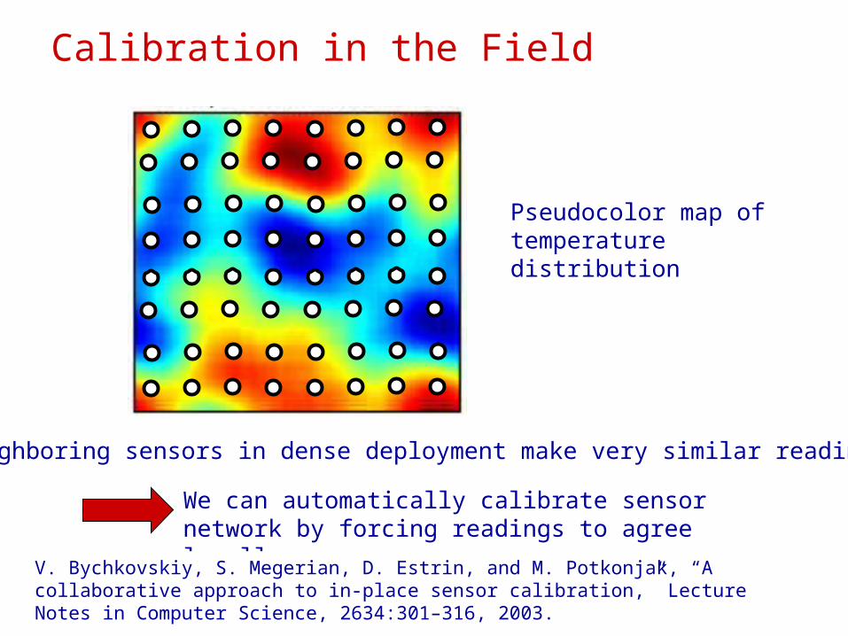
Calibration in the Field

Pseudocolor map of temperature distribution

Neighboring sensors in dense deployment make very similar readings

We can automatically calibrate sensor network by forcing readings to agree locally

V. Bychkovskiy, S. Megerian, D. Estrin, and M. Potkonjak, “A collaborative approach to in-place sensor calibration,” Lecture Notes in Computer Science, 2634:301–316, 2003.

Calibration by Local Agreement

space

Calibration via local agreement is based on assumption:

Linear deployment of sensors:

Ideal (calibrated) sensor readings:

These conditions define a signal subspace (constant functions)

Calibration by Local Agreement

space

Calibration via local agreement is based on assumption:

Linear deployment of sensors:

Ideal (calibrated) sensor readings:

These conditions define a signal subspace (constant functions)

Calibration assuming second derivatives are approx zero:

These conditions define a signal subspace (linear functions)

Signal Subspaces and Calibration

Calibration via signal subspace matching is based on assumption:

Ideal (calibrated) sensor readings:

Example of Constant Subspace:Example of Linear Subspace:

Signal Subspaces and Calibration

Calibration via signal subspace matching is based on assumption:

Ideal (calibrated) sensor readings:

P is called the orthogonal projection matrix corresponding to the orthogonal complement to the signal subspace

Ex: If the signal is a bandlimited signals, P projects onto the space outside of that band. If the signal is a “smooth” signal, P projects onto a the space of “rough” signals.

• The calibrated signals are a linear function of the uncalibrated snapshots:

• The calibrated signals lie in a known r-dimensional subspace of Rn

Assumptions

Let P denote the projection on to the orthogonal complement of the signal subspace, so Px = 0

Blind Calibration

k “snapshots” result in the following system of equations:

Which we can try to solve for and

…There is hope!

We now have a set of nk linear equations, and 2n unknowns. As long as there are enough linearly independent equations, we can solve for our unknowns!

Outline

• Preliminaries and Problem Formulation

• Approach and Intuition

• Identifiability

• Implications

• Proof of Gain Identifiability

• Simulations and Experiments

Identifiability Preview

We cannot identify the component of in the signal subspace. This component is indistinguishable from true signal.

However, since yi “modulates” , under certain

conditions on P it is possible exactly recover up to a scalar constant. We cannot distinguish between and (scalar constant) x .

Offsets:

Gains:

More explanation to come!

Matrix-Vector Formulation

Diag Operation:

System of Calibration Equations:

Then we must solve

However, the matrix P is rank n-r, so this equation gives us n-r equations and n unknowns.

There are r degrees of freedom– so if we calibrate (non-blind) only r sensor offsets, we can recover all of them!

Offset Solutions

Say we know α and let

Offset Solutions

where

Note:

• Every offset solution is a simple function of sensor data and gains

• If the true signals are zero-mean, and if we can estimate the gains correctly, then we correctly recover the offsets!

One possible estimate when we don’t know α would be:

Gain Solutions

A unique solution exists iff the matrix

has rank n-1 (i.e., a single vector in its right nullspace)

Exact Recovery of Calibration Gains

Assumptions:

Oversampling: The ideal sensor network signals lie in a known r-dimensional signal subspace

Randomness: The signals are random enough (for example, spread out over time so that they are changing) such that they are linearly independent

Incoherence: The signal subspace is incoherent with the canonical spatial basis (i.e., δ basis) (more on this in the proof)

When does have a unique solution?

Exact Recovery of Calibration Gains

Theorem 1: Under assumptions A1, A2 and A3, the gains can be perfectly recovered from any k ≥ r signal measurements by solving the linear system of equations

Theorem 2: If the signal subspace is defined by a subset of the DFT vectors (i.e., a frequency-domain subspace), then incoherence condition is automatically satisfied, and the gains can be perfectly recovered from any k ≥ 1 + (n-1)/(n-r) signal measurements

Outline

• Preliminaries and Problem Formulation

• Approach and Intuition

• Identifiability

• Implications

• Proof of Gain Identifiability

• Simulations and Experiments

ImplicationsWhat does it mean that we can perfectly recover the gains? These theorems have stated that it is possible to estimate the gain vector exactly under these assumptions.

Assumption A1 (Oversampling) is a given for slowly varying fields. This technique will not work for fields with spatial frequencies too high to be oversampled.

Assumption A2 (Randomness) is very reasonable, because it is possible to spread out measurements enough so that they are sufficiently different.

Assumption A3 (Incoherence) is easily checked and is met by commonly used subspaces like frequency subspaces and polynomial subspaces.

ImplicationsWhat does it mean that we can perfectly recover the gains? These theorems have stated that it is possible to estimate the gain vector exactly under these assumptions.

However, this theory has been carried out assuming signals are noise-free and assuming exact knowledge of the projection matrix P.

The Great News:There are computational ways to solve the system

of equations in the presence of noise and model error (not knowing P)!

In fact, many mathematical techniques have dealt with problems of system identification and blind equalization that can potentially be applied here.

ImplicationsWhat about the offsets? As we said, if the signals are zero-mean we can recover the offsets.

If the signals are not zero-mean, we need to collect r true offsets in order to calibrate all the offsets.

In the case of the Cold Air Drainage temperaturedata, we calibrated the transect on one side of the valley and found that r = 4.

So we only need to calibrate (non-blind) 4 sensors in order to discover all the sensor offsets!

Outline

• Preliminaries and Problem Formulation

• Approach and Intuition

• Identifiability

• Implications

• Proof of Gain Identifiability

• Simulations and Experiments

Proof Sketch

Oversampling: Signals lie in an r-dimensional subspace of Rn.

Randomness: k ≥ r snapshots span signal subspace with probability 1

Incoherence:

First, let α* be the true gains, and write system of equations in terms of calibrated signals

or equivalently

Proof Sketch

Calibration equations

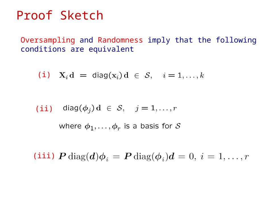
Proof Sketch

Oversampling and Randomness imply that the followingconditions are equivalent

(i)

(ii)

(iii)

Proof Sketch

(iii)

Let

Then the equation should have

only one solution, .

Invoke the assumption:

Thus, the single solution to our set of equations will be the true gains, α = α*

Incoherence Condition

What does it mean that this matrix has rank n-1 ?

What we know so far is that most frequency subspaces (low-pass, bandpass, high-pass) and polynomial subspaces (constant, linear, quadratic, etc) meet this condition.

It is an interesting question to ask: Why? And what other subspaces meet the condition?

Outline

• Preliminaries and Problem Formulation

• Approach and Intuition

• Identifiability

• Implications

• Proof of Gain Identifiability

• Simulations and Experiments

Robust Recovery of Calibration Gains

Gain equations may hold only approximately due to noise/errors:

Robust solutions:

Simulation Experiment

simulated temperature field 8x8 sensor readings

• field is smoothed GWN process

• approximate signal subspace = span of lowpass DFT vectors

Simulation Experiment

robust to noise

Error at 1% noise:

Gain: >.01%Offset: >2.4%

robust to mismodeling

Error at 10%:

Gain: >1%Offset: >4%

Simulation Experiment: Implementation

Estimating Gains

Partial information is best, but without information then the svd outperforms the least-squares method.

Estimating Offsets

Again, partial information is always best. Interestingly, when the signals are not zero-mean, LS does better even though it is using gains with more error!

Implementation Matters!

Sensing in the Box

Ideally all sensors should read the same temperature

1-d signal subspace of constant functions

time

sensor

warm

cool

Sensing in the Wild

temperature sensing at James Reserve

Sensing in the Wild

temperature sensing at James Reserve

4-dimensional signal subspace determined from calibrated sensor data

Future Work

• Noise analysis: From our formulations, we hope to derive bounds on blind calibration given a particular subspace P and a noise variance σ.

• Visiting the Cold Air Drainage sensors and calibrating them by hand was a cumbersome process. A hand-held device like the EcoPDA that could be carried to the sensors would be ideal. We could use it to show whether blind calibration can truly be done accurately with only r sensors.

• Model Uncertainty and Implementation: It isn’t clear how to proceed in order to understand how model uncertainty affects the output of blind calibration. More understanding of model errors on the singular value decomposition and optimization techniques is needed.

and possible collaboration topics

Conclusions• Sensor calibration gains and (partially) offsets can be determined from routine sensor measurements with some knowledge of calibrated signal characteristics (e.g., frequency band, smoothness)

• The key necessary condition is “incoherence” between signal subspace and canonical (spatial) basis; the condition is a nonlinear requirement on the signal basis and is easy to check in general

• Our experience is that solutions are robust to noise and mismodeling in some cases, and sensitive in others; we do not have a good understanding of the robustness of the methodology at this time

• Extensions are possible to handle more exotic calibration functions (e.g., nonlinear)

More info: Balzano and Nowak, “Blind Calibration of Sensor Networks,” IPSN 2007