Blind Super-Resolution Kernel Estimation using an Internal-GAN

Sefi Bell-Kligler Assaf Shocher Michal IraniDept. of Computer Science and Applied Math

The Weizmann Institute of Science, IsraelProject website: http://www.wisdom.weizmann.ac.il/∼vision/kernelgan

Abstract

Super resolution (SR) methods typically assume that the low-resolution (LR) imagewas downscaled from the unknown high-resolution (HR) image by a fixed ‘ideal’downscaling kernel (e.g. Bicubic downscaling). However, this is rarely the casein real LR images, in contrast to synthetically generated SR datasets. Whenthe assumed downscaling kernel deviates from the true one, the performance ofSR methods significantly deteriorates. This gave rise to Blind-SR – namely, SRwhen the downscaling kernel (“SR-kernel”) is unknown. It was further shownthat the true SR-kernel is the one that maximizes the recurrence of patches acrossscales of the LR image. In this paper we show how this powerful cross-scalerecurrence property can be realized using Deep Internal Learning. We introduce“KernelGAN”, an image-specific Internal-GAN [29], which trains solely on the LRtest image at test time, and learns its internal distribution of patches. Its Generatoris trained to produce a downscaled version of the LR test image, such that itsDiscriminator cannot distinguish between the patch distribution of the downscaledimage, and the patch distribution of the original LR image. The Generator, oncetrained, constitutes the downscaling operation with the correct image-specificSR-kernel. KernelGAN is fully unsupervised, requires no training data other thanthe input image itself, and leads to state-of-the-art results in Blind-SR when pluggedinto existing SR algorithms. 1

1 Introduction

The basic model of SR assumes that the low-resolution input image ILR is the result of down-scalinga high-resolution image IHR by a scaling factor s using some kernel ks (the "SR kernel"), namely:

ILR = (IHR ∗ ks) ↓s (1)

The goal is to recover IHR given ILR. This problem is ill-posed even when the SR-Kernel is assumedknown (an assumption made by most SR methods – older [8, 32, 7] and more recent [5, 20, 19, 21, 38,35, 12]). A boost in SR performance was achieved in the past few years introducing Deep-Learningbased methods [5, 20, 19, 21, 38, 35, 12]. However, since most SR methods train on syntheticallydownscaled images, they implicitly rely on the SR-kernel ks being fixed and ‘ideal’ (usually a Bicubicdownscaling kernel with antialiasing– MATLAB’s default imresize command). Real LR images,however, rarely obey this assumption. This results in poor SR performance by state-of-the-art(SotA) methods when applied to real or ‘non-ideal’ LR images (see Fig. 1a).

The SR kernel of real LR images is influenced by the sensor optics as well as by tiny camera motionof the hand-held camera, resulting in a different non-ideal SR-kernel for each LR image, even if takenby the same sensor. It was shown in [26] that the effect of using an incorrect SR-kernel is of greaterinfluence on the SR performance than any choice of an image prior. This observation was later shown

1Project funded by the European Research Council (ERC) under the Horizon 2020 research & innovationprogram (grant No. 788535)

arX

iv:1

909.

0658

1v6

[cs

.CV

] 7

Jan

202

0

(a) Comparison to SotA SR methods (SR×4):Since they train on ’ideal’ LR images, they perform poorly on real non-ideal LR images.

Bicubic EDSR+ RCAN+ KernelGAN(Ours) GroundTruth HRLR Input image interpolation [21] [38] SR method: [30]

(b) Comparison to SotA Blind-SR methods (SR×4):

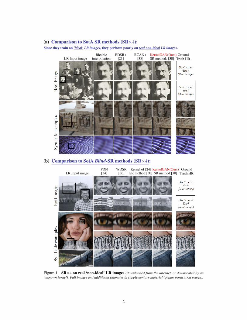
PDN WDSR Kernel of [24] KernelGAN(Ours) GroundTruth HRLR Input image [34] [36] SR method:[30] SR method:[30]

Figure 1: SR×4 on real ‘non-ideal’ LR images (downloaded from the internet, or downscaled by anunknown kernel). Full images and additional examples in supplementary material (please zoom in on screen).

2

to hold also for deep-learning based priors [30]. The importance of the SR-kernel accuracy wasfurther analyzed empirically in [27].

The problem of SR with an unknown kernel is known as Blind SR. Some Blind-SR methods [33, 17,14, 13, 3] were introduced prior to the deep learning era. Few Deep Blind-SR methods [34, 36] wererecently presented in the NTIRE’2018 SR challenge [31]. These methods do not explicitly calculatethe SR-kernel, but propose SR networks that are robust to variations in the downscaling kernel. Awork concurrent to ours, IKC [10], performs Blind-SR by alternating between the kernel estimationand the SR image reconstruction. A different family of recent Deep SR methods [30, 37], while notexplicitly Blind-SR, allow to input a different image-specific (pre-estimated) SR-kernel along withthe LR input image at test time. Note that SotA (non-blind) SR methods cannot make any use of animage-specific SR kernel at test time (even if known/provided), since it is different from the fixeddownscaling kernel they trained on. These methods thus produce poor SR results in realistic scenarios– see Fig. 1a (in contrast to their excellent performance on synthetically generated LR images).

The recurrence of small image patches (5x5, 7x7) across scales of a single image, was shown to be avery strong property of natural images [8, 39]. Michaeli & Irani [24] exploited this recurrence propertyto estimate the unknown SR-kernel directly from the LR input image. An important observationthey made was that the correct SR-kernel is also the downscaling kernel which maximizes thesimilarity of patches across scales of the LR image. Based on their observation, they proposed anearest-neighbor patch based method to estimate the kernel. However, their method tends to fail forSR scale factors larger than ×2, and has a very long runtime.

This internal cross-scale recurrence property is very powerful, since it is image-specific and unsu-pervised (requires no prior examples). In this paper we show how this property can be combinedwith the power of Deep-Learning, to obtain the best of both worlds – unsupervised SotA SR-kernelestimation, with SotA Blind-SR results. We build upon the recent success of Deep Internal Learn-ing [30] (training an image-specific CNN on examples extracted directly from the test image), and inparticular on Internal-GAN [29] – a self-supervised GAN which learns the image-specific distributionof patches.

More specifically, we introduce "KernelGAN" – an image-specific Internal-GAN, which estimates theSR kernel that best preserves the distribution of patches across scales of the LR image. Its Generatoris trained to produce a downscaled version of the LR test image, such that its Discriminator cannotdistinguish between the patch distribution of the downscaled image, and the patch distributionof the original LR image. In other words, G trains to fool D to believe that all the patches ofthe downscaled image were actually taken from the original one. The Generator, once trained,constitutes the downscaling operation with the correct image-specific SR-kernel. KernelGAN isfully unsupervised, requires no training data other than the input image itself, and leads to state-of-the-art results in Blind-SR when plugged into existing SR algorithms.

Since downscaling by the SR-kernel is a linear operation applied to the LR image (convolution andsubsampling – see Eq. 1), our Generator (as opposed to the Discriminator) is a linear network (withoutnon-linear activations). At first glance, it may seem that a single-strided convolution layer (whichstems from Eq. 1) should suffice as a Generator. Interestingly, we found that using a deep linearnetwork is dramatically superior to a single-strided one. This is consistent with recent findings intheoretical deep-learning [28, 2, 18, 11], where deep linear networks were shown to have optimizationadvantages over a single layer network for linear regression models. This is further elaborated inSec. 4.1.

Our contributions are therefore several-fold:

• This is the first dataset-invariant deep-learning method to estimate the unknown SR kernel (acritical step for true SR of real LR images). KernelGAN is fully unsupervised and requires notraining data other than the input image itself, hence enables true SR in "the wild".

• KernelGAN leads to state-of-the-art results in Blind-SR when plugged into existing SR algorithms.• To the best of our knowledge, this is the first practical use for deep linear networks (so far used

mostly for theoretical analysis), with demonstrated practical advantages.

3

Figure 2: KernelGAN: The patch GAN trains on patches of a single input image (real). D tries to distinguishreal patches from those generated by G (fake). G learns to downscale X2 the image while fooling D i.e.maintaining the same distribution of patches. Both networks are fully convolutional, which in the case of imagesimplies that each pixel in the output is a result of a specific receptive field (i.e. patch) in the input.

2 Overview of the Approach

Given only the input image, our goal is to find its underlying image-specific SR kernel. We seek thekernel that best preserves the distribution of patches across scales of the LR image. More specifically,we aim to "generate" a downscaled image (e.g. by a factor of 2) such that its patch distribution is asclose as possible to that of the LR image.

By matching distributions rather than individual patches, we can leverage recent advances in dis-tribution modeling using Generative Adversarial Networks (GANs) [9]. GANs can be understoodas a tool for distribution matching [9]. A GAN typically learns a distribution of images in a largeimage dataset. It maps examples from a source distribution, px, to examples indistinguisable froma target distribution, py: G : x→ y with x∼px, and G(x)∼py. An internal GAN [29] trains on asingle input image and learns its unique internal distribution of patches.

Inspired by InGAN [29], KernelGAN is also an image specific GAN that trains on a single inputimage. It consists of a downscaling generator (G) and a discriminator (D) as depicted in Fig. 2. BothG and D are fully-convolutional, which implies the network is applied to patches rather than thewhole image, as in [16]. Given an input image ILR, G learns to downscale it, such that, for D, at thepatch level, it is indistinguishable from the input image ILR.

D trains to output a heat map, referred to as D-map (see fig. 2) indicating for each pixel, how likelyis its surrounding patch to be drawn from the original patch-distribution. It alternately trains onreal examples (crops from the input image) and fake ones (crops from G’s output). The loss is thepixel-wise MSE difference between the output D-map and the label map. The labels for training Dare a map of all ones for crops extracted from the original LR image, and a map of all zeros for cropsextracted from the downscaled image.

We adopt a variant of the LSGAN [23] with the L1 Norm, and define the objective of KernelGAN as:G∗(ILR) = argmin

GmaxD

{Ex∼patches(ILR)[|D(x)− 1|+ |D(G(x)))|] +R

}(2)

whereR is the regularization term on the downscaling SR-kernel resulting from the generator G (seemore details in Sec. 4.2). Once converged, the generator G∗ constitutes, implicitly, the ideal SRdownscaling function for the specific LR image.The GAN trains for 3,000 iterations, alternating single optimization steps of G and D, with theADAM optimizer (β1 = 0.5, β2 = 0.999). Learning rate is 2e−4, decaying ×0.1 every 750 iters.

3 Discriminator

The goal of the discriminator D is to learn the distribution of patches of the input image ILR anddiscriminate between real patches belonging to this distribution and fake patches generated by G.D’s real examples are crops from ILR, while fake examples are crops currently outputed by G.

We use a fully-convolutional patch discriminator, as introduced in [16], applied to learn the patchdistribution of a single image as in [29]. To discriminate small image patches, we use no pooling

4

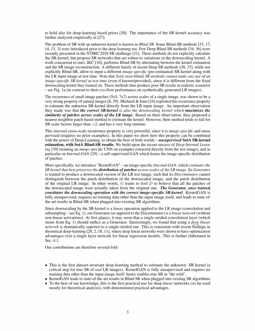
Figure 3: Fully Convolutional PatchDiscriminator: A 7×7 convolution filterfollowed by six 1×1 convolutions, includ-ing Spectral normalization [25], Batchnormalization [15], ReLU and a Sigmoidactivations. An input crop of 32×32 re-sults with a 32×32 map∈ [0,1].

or strides, thus achieving a small receptive field of a 7×7 patch. In this setting, D is implicitlyapplied to each patch separately and produces a heat-map (D-map) where each location in the mapcorresponds to a patch from the input. The labels for the discriminator are maps (matrices of real/fake,i.e. 1/0 labels, respectively) of the same size as the input to the discriminator. Each pixel in D-mapindicates how likely is its surrounding patch to be drawn from the learned patch distribution. SeeFig. 3 for architecture details of the discriminator.

4 Deep Linear Generator = The downscaling SR-Kernel

4.1 Deep Linear GeneratorThe generator G constitutes the downscaling model. Since downscaling by convolution and subsam-pling is a linear transform (Fig. 1), we use a linear Generator (without any non-linear activations).We refer to the model of downscaling from Eq. 1. In principle, the expressiveness of a single stridedconvolutional layer should cover all possible downscaling methods captured by Eq. 1. However, weempirically found that such architecture does not converge to the correct solution (see 6). We attributethis behavior to the following conjecture: A generator consisting of a single layer has exactly one setof parameters for the correct solution (the set of weights that make the ground-truth kernel). Thismeans that there is only one point on the optimization surface that is acceptable as a solution and it isthe global minimum. Achieving such a global minimum is easy when the loss function is convex(as in linear regression). But in our case the overall loss function is a non-linear neural network-D which is highly non-convex. In such case, the probability for getting from some random initialstate to the global minimum using gradient based methods is negligible. In contrast to a single layer,standard (deep) neural networks are assumed to converge from a random initialization due to the factthat there are many good local minima and negligibly few bad local minima [6, 18]. Hence, for aproblem that by definition has one valid solution, optimizing a single layer generator is impossible.

A non-linear generator would not be suitable either. Without an explicit constraint on G to be linear,it will generate physically unwanted solutions for the optimization objective. Such solutions includegenerating any image that contains valid patches but has no downscaling relation (Eq. 1). Oneexample is generating a tile of just several patches from the input. This would be a solution thatcomplies with eq. 2 but is unwanted.

This conjecture motivated us to use deep linear networks. These are networks consisting of asequence of linear layers with no activations, and are used for theoretical analysis [28, 2, 18, 11].The expressiveness of a deep linear network is exactly as the one of a single linear layer (i.e. Linearregression), however, its optimization has several different aspects. While it can be convex withrespect to the input, the loss would never be convex with respect to the weights (assuming more thanone layer). In fact, linear networks have infinitely many equally valued global minima. Any choice ofnetwork parameters matching to one of these minima would be equivalent to any other minimum point-they are just different factorizations of the same matrix. Motivated by these observations, we employa deep linear generator. By that we allow infinitely many valid solutions to our optimization objective,all equivalent to the same linear solution. Furthermore, it was shown by [2], that gradient-basedoptimization is faster for deeper linear networks than shallow ones.

Fig. 4 depicts the architecture of G. We use 5 hidden convolutional layers with 64 channels each.The first 3 filters are 7×7, 5×5, 3×3 and the rest are 1×1. This makes a receptive field of 13 ×13(allowing for a 13 × 13 SR kernel). This setting of filters takes into account the effective receptivefield [22]; maintaining the same receptive field while having filters bigger than 1×1 following thefirst layer encourages the center of the kernel to have higher values. To provide a reasonable initialstarting point, the generator’s output is constrained to be similar to an ideal downscaling (e.g. bicubic)of the input, for the first iterations. Once satisfied, this constraint is discarded.

5

Figure 4: Deep linear G: A 6 layerconvolutional network without non-linear activations.The deep linear network on the left hasequal expressiveness power as the sin-gle strided convolution downscalingmodel, on the right.

4.2 Extracting the explicit kernelAt any iteration during the training, the generator G constitutes the currently estimated downscalingoperation for the specific LR input image. The image-specific kernel is implicitly captured by thetrained weights of G. However, there are two reasons to explicitly extract the kernel from G. First,we are interested in having a compact downscaling convolution kernel rather than a downscalingnetwork. This step is trivial; convolving all the filters of G sequentially with sride 1 results in theSR-kernel k (see Fig. 4). When extracted, the kernel is just a small array that can be supplied toSR algorithms. The second reason for explicitly extracting the kernel is to allow applying explicitand physically-meaningful priors on the kernel. This is the goal of the regularization term R inEq.2 which decreases the hypotheses space to a sub-set of the plausible kernels, that obey certainrestrictions. Such restrictions are that the kernel would sum up to 1 and be centered so it will notshift the image. The regularization also ameliorates faulty tendencies of the optimization process toproduce kernels that are too spread out and smooth. However, it is not enough to extract the kernel,this extraction must be differentiable so that the regularization losses can be back-propagated throughit. At each iteration, we apply a differentiable action of calculating the kernel (convolving all thefilters of G sequentially with stride-1). The regularization loss termR is then applied and included inthe optimization objective.

The regularization term in our objective in eq. 2 is the following:

R = αLsum_to_1 + βLboundaries + γLsparse + δLcenter (3)

where α = 0.5, β = 0.5, γ = 5, δ = 1, and:

• Lsum_to_1 =∣∣∣1−∑i,j ki,j

∣∣∣ encourages k to sum to 1.• Lboundaries =

∑i,j |ki,j ·mi,j | penalizing non-zero values close to the boundaries. m is a

constant mask of weights exponentially growing with distance from the center of k.• Lsparse =

∑i,j |ki,j |

1/2 encourages sparsity to prevent the network from oversmoothing kernels.

• Lcenter =∥∥∥(x0, y0)− ∑

i,j ki,j ·(i,j)∑i,j ki,j

∥∥∥2

encourages k’s center of mass to be at the center of thekernel, where (x0, y0) denote the center indices.

SR kernels are not only image specific, but also depend on the desired scale-factor s. However,there is a simple relation between SR-kernels of different scales. We are thus able to obtain akernel for SR ×4 from G that was trained to downscale by ×2. This is advantageous for tworeasons: First, it allows extracting kernels for various scales by one run of KernelGAN. Second,it prevents downscaling the LR image too much. Small LR images downscaled by a scale factorof 4 may result in tiny images (×16 smaller than the HR image) which may not contain enoughdata to train on. KernelGAN is trained to estimate a kernel k2 for a scale-factor of 2. It is easyto show that the kernel for a scale factor of 4, i.e. k4, can be analytically calculated by requiring:ILR ∗ k4 ↓4= (ILR ∗ k2 ↓2) ∗ k2 ↓2.It implies that k4 = k2 ∗ k2_dilated , where k2_dilated[n1, n2] =

{k2[n1

2 ,n2

2

]n1, n2 even

0 elseFor a mathematical proof of the above derivation, as well as an ablation study of the various kernelconstraints – see our project website.

5 Experiments and resultsWe evaluated our method on real LR images, as well as on ‘non-ideal’ synthetically generated LRimages with ground-truth (both ground-truth HR images, as well as the true SR-kernels).

6

Figure 5: SR kernel estimation: We compareground truth kernel, Michaeli and Irani [24]and KernelGAN (ours). PSNR of ZSSR [30],when supplied with those kernels, is noted inthe bottom right of each kernel, emphasizing thesignificance of kernel estimation accuracy. Ourmethod outperforms [24] in SR performance (aswell as in visual similarity to ground truth SR kernel)

Method ×2 ×4Class 1: Bicubic Interpolation 28.731 / 0.8040 25.330 / 0.6795

SotA SR algorithms Bicubic kernel + ZSSR [30] 29.102 / 0.8215 25.605 / 0.6911(trained on bicubically EDSRplus [21] 29.172 / 0.8216 25.638 / 0.6928downscaled images) RCANplus [38] 29.198 / 0.8223 25.659 / 0.6936

Class 2: PDN [34] - 1st in NTIRE track4 - 26.340 / 0.7190Blind-SR WDSR [36] - 1st in NTIRE track2 - 21.546 / 0.6841

NTIRE’18 [31] WDSR [36] - 1st in NTIRE track3 - 21.539 / 0.7016winners WDSR [36] - 2nd in NTIRE track4 - 25.636 / 0.7144Class 3: Michaeli & Irani [24] + SRMD [37] 25.511 / 0.8083 23.335 / 0.6530

kernel estimation Michaeli & Irani [24] + ZSSR [30] 29.368 / 0.8370 26.080 / 0.7138+ KernelGAN (Ours) + SRMD [37] 29.565 / 0.8564 25.711 / 0.7265

non Blind-SR algorithm KernelGAN (Ours) + ZSSR [30] 30.363 / 0.8669 26.810 / 0.7316Class 4: Ground-truth kernel + SRMD [37] 31.962 / 0.8955 27.375 / 0.7655

Upper bound Ground-truth kernel + ZSSR [30] 32.436 / 0.8992 27.527 / 0.7446

Table 1: SotA SR performance (PSNR(dB) / SSIM) on 100 images of DIV2KRK (sec. 5.2) . Red indicates thebest performance, blue indicates second best.

5.1 Evaluation MethodThe performance of our method is analyzed in 2 ways: Kernel estimation accuracy and SR perfor-mance. The latter is done both visually (see fig. 1a and supplementary material), and empirically onthe synthetic dataset analyzing PSNR and SSIM measurements (Table 1). Evaluation is done usingthe script provided by [19] and used by many works, including [30, 20, 21]. For evaluation of thekernel estimation we chose two non-blind SR algorithms that accept a SR-kernel as input [30, 37],provide them with different kernels (bicubic, ground truth SR-kernel, ours and [30]) and comparedtheir SR performance. We present four types (categories) of algorithms for the analysis:

• Type 1 includes the non-blind SotA SR methods trained on bicubically downscaled images.• Type 2 are the winners of the NTIRE’2018 Blind-SR challenge [31].• Type 3 consists of combinations of 2 methods for SR-kernel estimation, [24] and ours, and 2

non-blind SR methods, [30, 37], that regard the estimated kernel as input. This combination isitself, a full Blind-SR algorithm.

• Type 4, is again the combination above, only with the use of the ground truth SR-kernel, thusproviding an upper bound to Type 3.

When providing a kernel to ZSSR [30] (whether ours, [24]’s, ground-truth kernel), we provide boththe ×2 and ×4 kernels, in order to exploit the gradual process of ZSSR (using 2 sequential SR steps).

We compare our kernel estimation to Michaeli & Irani [24] which, to the best of our knowledge, isthe leading method for SR-kernel estimation from a single image.

5.2 Dataset for Blind-SRThere is no adequate dataset for quantitatively evaluating Blind-SR. The data used in the NTIRE’2018Blind-SR challenge [31] has an inherent problem; it suffers from sub-pixel misalignments betweenthe LR image and the HR ground truth, resulting in subpixel misalignments between the reconstructedSR images and the HR ground truth images. Such small misalignments are known to prefer (i.e.give lower error to) blurry images over sharp ones. A different benchmark suggested by [4] is notyet available, and is only restricted to 3 SR blur kernels. As a result, we generated a new Blind-SRbenchmark, referred to as DIV2KRK (DIV2K random kernel).

7

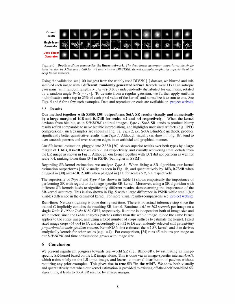
Figure 6: Depth is of the essence for the linear network: The deep linear generator outperforms the singlelayer version by 3.8dB and 1.6dB for ×2 and ×4 over DIV2KRK. Kernel examples emphasize superiority of thedeep linear network.

Using the validation set (100 images) from the widely used DIV2K [1] dataset, we blurred and sub-sampled each image with a different, randomly generated kernel. Kernels were 11x11 anisotropicgaussians with random lengths λ1, λ2∼U(0.6, 5) independently distributed for each axis, rotatedby a random angle θ∼U [−π, π]. To deviate from a regular gaussian, we further apply uniformmultiplicative noise (up to 25% of each pixel value of the kernel) and normalize it to sum to one. SeeFigs. 5 and 6 for a few such examples. Data and reproduction code are available on project website.

5.3 ResultsOur method together with ZSSR [30] outperforms SotA SR results visually and numericallyby a large margin of 1dB and 0.47dB for scales ×2 and ×4 respectively. When the kerneldeviates from bicubic, as in DIV2KRK and real images, Type 1, SotA SR, tends to produce blurryresults (often comparable to naive bicubic interpolation), and highlights undesired artifacts (e.g. JPEGcompression), such examples are shown in Fig. 1a. Type 2, i.e. SotA Blind-SR methods, producesignificantly better quantitative results, than Type 1. Although visually (as shown in Fig. 1b), tend toover-smooth patterns and over-sharpen edges in an artificial and graphical manner.

Our SR-kernel estimation, plugged into ZSSR [30], shows superior results over both types by a largemargin of 1.1dB, 0.47dB for scales ×2, ×4 respectively, and visually recovering small details fromthe LR image as shown in Fig 1. Although, our kernel together with [37] did not perform as well forscale ×4, ranking lower than [34] in PSNR (but higher in SSIM).

Regarding SR-kernel estimation, we analyze Type 3. When fixing a SR algorithm, our kernelestimation outperforms [24] visually, as seen in Fig. 1b, and quantitatively by 1dB, 0.73dB whenplugged in [30] and 4dB, 2.3dB when plugged in [37] for scales ×2, ×4 respectively.

The superiority of Type 3 and Type 4 (as shown in Table 1) shows empirically the importance ofperforming SR with regard to the image specific SR-kernel. Moreover, using a SR algorithm withdifferent SR-kernels leads to significantly different results, demonstrating the importance of theSR-kernel accuracy. This is also shown in Fig. 5 with a large difference in PSNR while small (butvisible) difference in the estimated kernel. For more visual results+comparisons see project website.

Run-time: Network training is done during test time. There is no actual inference step since thetrained G implicitly contains the resulting SR-kernel. Runtime is 61 or 102 seconds per image on asingle Tesla V-100 or Tesla K-80 GPU, respectively. Runtime is independent both of image size andscale factor, since the GAN analyzes patches rather than the whole image. Since the same kernelapplies to the entire image, analyzing a fixed number of crops suffices to estimate the kernel. Fixedsized image crops (64×64 to G, and accordingly 32×32 to D) are randomly selected with probabilityproportional to their gradient content. KernelGAN first estimates the ×2 SR-kernel, and then derivesanalytically kernels for other scales (e.g., ×4). For comparison, [24] runs 45 minutes per image onour DIV2KRK and time consumption grows with image size.

6 ConclusionWe present significant progress towards real-world SR (i.e., Blind-SR), by estimating an image-specific SR-kernel based on the LR image alone. This is done via an image-specific internal-GAN,which trains solely on the LR input image, and learns its internal distribution of patches withoutrequiring any prior examples. This gives rise to true SR "in the wild". We show both visuallyand quantitatively that when our kernel estimation is provided to existing off-the-shelf non-blind SRalgorithms, it leads to SotA SR results, by a large margin.

8

References[1] Eirikur Agustsson and Radu Timofte. Ntire 2017 challenge on single image super-resolution: Dataset and

study. In The IEEE Conference on Computer Vision and Pattern Recognition (CVPR) Workshops, July2017.

[2] Sanjeev Arora, Nadav Cohen, and Elad Hazan. On the optimization of deep networks: Implicit accelerationby overparameterization. In Jennifer G. Dy and Andreas Krause, editors, ICML, volume 80 of Proceedingsof Machine Learning Research, pages 244–253. PMLR, 2018.

[3] Isabelle Begin and Frank P. Ferrie. Blind super-resolution using a learning-based approach. In InternationalConference on Pattern Recognition, ICPR ’04, Washington, DC, USA, 2004. IEEE Computer Society.

[4] Jianrui Cai, Hui Zeng, Hongwei Yong, Zisheng Cao, and Lei Zhang. Toward real-world single imagesuper-resolution: A new benchmark and a new model, 2019.

[5] Kaiming He Xiaoou Tang Chao Dong, Chen Change Loy. Learning a deep convolutional network forimage super-resolution. In European Conference on Computer Vision (ECCV), 2014.

[6] Anna Choromanska, MIkael Henaff, Michael Mathieu, Gerard Ben Arous, and Yann LeCun. The LossSurfaces of Multilayer Networks. In Guy Lebanon and S. V. N. Vishwanathan, editors, Proceedings of theEighteenth International Conference on Artificial Intelligence and Statistics, volume 38 of Proceedings ofMachine Learning Research, pages 192–204, San Diego, California, USA, 09–12 May 2015. PMLR.

[7] Gilad Freedman and Raanan Fattal. Image and video upscaling from local self-examples. ACM Trans.Graph., April 2011.

[8] Daniel Glasner, Shai Bagon, and Michal Irani. Super-resolution from a single image. In ICCV, 2009.

[9] Ian Goodfellow, Jean Pouget-Abadie, Mehdi Mirza, Bing Xu, David Warde-Farley, Sherjil Ozair, AaronCourville, and Yoshua Bengio. Generative adversarial nets. In Z. Ghahramani, M. Welling, C. Cortes,N. D. Lawrence, and K. Q. Weinberger, editors, Advances in Neural Information Processing Systems 27,pages 2672–2680. Curran Associates, Inc., 2014.

[10] Jinjin Gu, Hannan Lu, Wangmeng Zuo, and Chao Dong. Blind super-resolution with iterative kernelcorrection. In The IEEE Conference on Computer Vision and Pattern Recognition (CVPR), June 2019.

[11] Moritz Hardt and Tengyu Ma. Identity matters in deep learning. CoRR, abs/1611.04231, 2016.

[12] Muhammad Haris, Greg Shakhnarovich, and Norimichi Ukita. Deep back-projection networks for super-resolution. In IEEE Conference on Computer Vision and Pattern Recognition (CVPR), 2018.

[13] He He and Wan-Chi Siu. Single image super-resolution using gaussian process regression. In Proceedingsof the 2011 IEEE Conference on Computer Vision and Pattern Recognition, CVPR ’11, pages 449–456,Washington, DC, USA, 2011. IEEE Computer Society.

[14] Yu He, Kim-Hui Yap, Li Chen, and Lap-Pui Chau. A soft map framework for blind super-resolution imagereconstruction. Image Vision Comput., 27(4):364–373, March 2009.

[15] Sergey Ioffe and Christian Szegedy. Batch normalization: Accelerating deep network training by reducinginternal covariate shift. In Proceedings of the 32Nd International Conference on International Conferenceon Machine Learning - Volume 37, ICML’15, pages 448–456. JMLR.org, 2015.

[16] Phillip Isola, Jun-Yan Zhu, Tinghui Zhou, and Alexei A Efros. Image-to-image translation with conditionaladversarial networks. The IEEE Conference on Computer Vision and Pattern Recognition (CVPR), 2017.

[17] Neel Joshi, Richard Szeliski, and David J. Kriegman. Psf estimation using sharp edge prediction. 2008IEEE Conference on Computer Vision and Pattern Recognition, pages 1–8, 2008.

[18] Kenji Kawaguchi. Deep learning without poor local minima. In D. D. Lee, M. Sugiyama, U. V. Luxburg,I. Guyon, and R. Garnett, editors, Advances in Neural Information Processing Systems 29, pages 586–594.Curran Associates, Inc., 2016.

[19] Jiwon Kim, Jung Kwon Lee, and Kyoung Mu Lee. Accurate image super-resolution using very deepconvolutional networks. In The IEEE Conference on Computer Vision and Pattern Recognition (CVPR)Workshops, pages 1646–1654, 06 2016.

[20] Jiwon Kim, Jung Kwon Lee, and Kyoung Mu Lee. Deeply-recursive convolutional network for imagesuper-resolution. In The IEEE Conference on Computer Vision and Pattern Recognition (CVPR Oral),June 2016.

9

[21] Bee Lim, Sanghyun Son, Heewon Kim, Seungjun Nah, and Kyoung Mu Lee. Enhanced deep residualnetworks for single image super-resolution. In The IEEE Conference on Computer Vision and PatternRecognition (CVPR) Workshops, July 2017.

[22] Wenjie Luo, Yujia Li, Raquel Urtasun, and Richard Zemel. Understanding the effective receptive field indeep convolutional neural networks. In D. D. Lee, M. Sugiyama, U. V. Luxburg, I. Guyon, and R. Garnett,editors, Advances in Neural Information Processing Systems 29, pages 4898–4906. Curran Associates,Inc., 2016.

[23] Xudong Mao, Qing Li, Haoran Xie, Raymond Y. K. Lau, and Zhen Wang. Least squares generativeadversarial networks. In Computer Vision (ICCV), IEEE International Conference on, 2017.

[24] T. Michaeli and M. Irani. Nonparametric blind super-resolution. In International Conference on ComputerVision (ICCV), 2013.

[25] Takeru Miyato, Toshiki Kataoka, Masanori Koyama, and Yuichi Yoshida. Spectral normalization forgenerative adversarial networks. In International Conference on Learning Representations, 2018.

[26] Alexander Apartsin Boaz Nadler Anat levin Netalee Efrat, Daniel Glasner. Accurate blur models vs. imagepriors in single image super-resolution. In ICCV, 2013.

[27] G. Riegler, S. Schulter, M. Rüther, and H. Bischof. Conditioned regression models for non-blind singleimage super-resolution. In 2015 IEEE International Conference on Computer Vision (ICCV), pages522–530, Dec 2015.

[28] Andrew M. Saxe, James L. McClelland, and Surya Ganguli. Exact solutions to the nonlinear dynamics oflearning in deep linear neural networks, 2013.

[29] Assaf Shocher, Shai Bagon, Phillip Isola, and Michal Irani. Ingan: Capturing and remapping the “dna” ofa natural image. In arXiv, 2019.

[30] Assaf Shocher, Nadav Cohen, and Michal Irani. Zero-shot super-resolution using deep internal learning.In The IEEE Conference on Computer Vision and Pattern Recognition (CVPR), 2018.

[31] Radu Timofte, Shuhang Gu, Jiqing Wu, Luc Van Gool, Lei Zhang, Ming-Hsuan Yang, Muhammad Haris,et al. Ntire 2018 challenge on single image super-resolution: Methods and results. In The IEEE Conferenceon Computer Vision and Pattern Recognition (CVPR) Workshops, June 2018.

[32] Radu Timofte, Vincent De Smet, and Luc Van Gool. A+: Adjusted anchored neighborhood regression forfast super-resolution. In ACCV, 2014.

[33] Qiang Wang, Xiaoou Tang, and Harry Shum. Patch based blind image super resolution. In Proceedings ofthe Tenth IEEE International Conference on Computer Vision (ICCV’05) Volume 1 - Volume 01, ICCV ’05,pages 709–716, Washington, DC, USA, 2005. IEEE Computer Society.

[34] Wang Xintao, Yu Ke, Hui Tak-Wai, Dong Chao, Lin Liang, and Change Loy Chen. Deep poly-densenetwork for image superresolution. NTIRE challenge, 2018.

[35] W. Yifan, F. Perazzi, B. McWilliams, A. Sorkine-Hornung, O Sorkine-Hornung, and C. Schroers. A fullyprogressive approach to single-image super-resolution. In CVPR Workshops, June 2018.

[36] Jiahui Yu, Yuchen Fan, Jianchao Yang, Ning Xu, Zhaowen Wang, Xinchao Wang, and Thomas S. Huang.Wide activation for efficient and accurate image super-resolution. CoRR, abs/1808.08718, 2018.

[37] Kai Zhang, Wangmeng Zuo, and Lei Zhang. Learning a single convolutional super-resolution network formultiple degradations. In IEEE Conference on Computer Vision and Pattern Recognition, pages 3262–3271,2018.

[38] Yulun Zhang, Kunpeng Li, Kai Li, Lichen Wang, Bineng Zhong, and Yun Fu. Image super-resolutionusing very deep residual channel attention networks. In ECCV, 2018.

[39] Maria Zontak and Michal Irani. Internal statistics of a single natural image. In The IEEE Conference onComputer Vision and Pattern Recognition (CVPR), 2011.

10