UGMM-101 Differential Calculus BLOCK-1 SET, RELATION, FUNCTION AND ITS PROPERTY 03-130 UNIT-1 Set and Relation 05-36 UNIT-2 Functions 37-78 UNIT-3 Limits 79-110 UNIT-4 Continuity 111-130 BLOCK-2 DIFFERENTIAL CALCULUS 131-232 UNIT-5 Differentiability and derivatives 133-160 UNIT-6 Derivative of hyperbolic functions and some special 161-192 Functions UNIT-7 Successive differentiation 193-218 UNIT-8 Mean value theorems 219-232 Uttar Pradesh Rajarshi Tandon Open University DIFFERENTIAL CALCULUS UGMM-101/1
Transcript
UGMM-101Differential Calculus
BLOCK-1 SET, RELATION, FUNCTION AND ITS PROPERTY 03-130
UNIT-1 Set and Relation 05-36 UNIT-2 Functions 37-78 UNIT-3 Limits 79-110 UNIT-4 Continuity 111-130
BLOCK-2 DIFFERENTIAL CALCULUS 131-232 UNIT-5 Differentiability and derivatives 133-160
UNIT-6 Derivative of hyperbolic functions and some special 161-192 Functions
UNIT-7 Successive differentiation 193-218 UNIT-8 Mean value theorems 219-232
Uttar Pradesh Rajarshi Tandon Open University
DIFFERENTIAL CALCULUS
UGMM-101/1
Curriculum Design Committee Prof. K.N. Singh Vice Chancellor Uttar Pradesh Rajarshi Tandon Open University Dr. Ashutosh Gupta Chairman Director, School of Science, UPRTOU, Prayagraj Prof. Sudhir Srivastava Member Professor, Dept. of Mathematics, Pt. Deen Dayal Upadhyay University, Gorakhpur, University Prof. P.K. Singh Member Dept. of Mathematics, University of Allahabad, Prayagraj Prof. Mona Khare Member Dept. of Mathematics, University of Allahabad, Prayagraj Dr. A.K. Pandey Member Associate Professor, E.C.C. University of Allahabad, Prayagraj Dr. Vikas Singh Member Academic Consultant, School of Science, UPRTOU, Prayagraj Dr. S. S. Tripathi Member Academic Consultant, School of Science, UPRTOU, Prayagraj
Course Preparation Committee Dr. Vikas Singh Author Academic Consultant, (Block-1 (Unit-1), Block-2, (Unit-7, 8) School of Science, UPRTOU, Prayagraj Dr. Yasmin Begawadi Author Assistant Professor, Symbiosis University, Pune (Block-1 (Unit-2,3,4), Block-2, (Unit-5, 6) Dr. S.S. Tripathi Editor Academic Consultant, School of Science, UPRTOU, Prayagraj. Dr. Ashutosh Gupta, Chairman Director, School of Computer and Information Science, UPRTOU, Prayagraj
Faculty Members, School of Sciences Dr. Ashutosh Gupta, Director, School of Science, UPRTOU, Prayagraj. Dr. Shruti, Asst. Prof. (Statistics), School of Science, UPRTOU, Prayagraj Dr. Marisha Asst. Prof. (Computer Science), School of Science, UPRTOU, Prayagraj Mr. Manoj K Balwant Asst. Prof. (Computer Science), School of Science, UPRTOU, Prayagraj Dr. Dinesh K Gupta Academic Consultant (Chemistry), School of Science, UPRTOU, Prayagraj Dr. S.S. Tripathi, Academic Consultant (Maths), School of Science, UPRTOU, Prayagraj Dr. Dharamveer Singh, Academic Consultant (Bio-Chemistry), School of Science, UPRTOU, Prayagraj Dr. R.P. Singh, Academic Consultant (Bio-Chemistry), School of Science, UPRTOU, Prayagraj Dr. Susma Chauhan, Academic Consultant (Botany), School of Science, UPRTOU, Prayagraj Dr. Deepa Chaubey, Academic Consultant (Zoology), School of Science, UPRTOU, Prayagraj Dr. Arvind Kumar Mishra, Academic Consultant (Physics), School of Science, UPRTOU, Prayagraj
1.7 Venn diagram 1.8 Cartesian product of two sets
1.9 Relation, Definition and Examples
1.10 Domain and Range of a Relation
1.11 Types of Relations in a set
1.12 Composition of Relation
1.13 Equivalence relation in a set
1.14 Partition of a Set
1.15 Quotient set of a set
1.16 Oder Relation and Examples
1.17 Summary
1.1. INTRODUCTION
The notations and terminology of set theory which was originated in the year 1895 by the German mathematician G. Cantor. In our daily life, we often use phrases of words such as a bunch of keys, a pack of cards, a class of students, a team of players, etc. The words bunch, pack, class and team all denote a collection of several discrete objects. Also, the dictionary meaning of set is a group or a collection of distinct, definite and distinguishable objects selected by means of some rules or description.
In this unit we will introduce set and various examples of sets. Then we will discuss types and some operations on sets. We will also UGMM-101/5
Set, Relation, Function And Its Property
introduce Venn diagrams, a pictorial way of describing sets. Cartesian product of two sets, relation, equivalence relation, order relation, equivalence class, partition of a set. Knowledge of the material covered in this unit is necessary for studying any mathematics course, so please study this unit carefully.
Objectives After studying this unit you should be able to:
Use the notation of set theory;
Find the union, intersection, difference, complement, and Cartesianproduct of sets;
Identify a set, represent sets by the listing method, propertymethod and Venn diagrams;
Prove set identities, and apply De Morgan’s laws;
Recall the basic properties of relations;
Derive other properties with the help of the basic ones;
Identify various types of relations;
Understand the relationship between equivalence classes andpartition;
1.2 Set Theory
It was first of all used by George Cantor. According to him, ‘A set is any collection into a whole of definite and distinct objects of our intuition or thought’. However, Cantor’s definition faced controversies due to the forms like ‘definite’ and ‘collection into a whole’. Later on, a single word ‘distinguishable’ used to make the definition acceptable. ‘A set is any collection of distinct and distinguishable objects around us’. By the form ‘distinct’, we mean that no object is repeated and some lack the term ‘distinguishable’ we mean that whether that object is in our collection or not. The objects belonging to a set are called as elements or members of that set. For example, say A is a set of stationary used by any student i.e.
A = {Pen, Pencil, Eraser, Sharpener, Paper}
A set is represented by using all its elements between bracket {} and by separating them from each other by commas (if there are more than one element). As we have seen sets are denoted by capital letters of English alphabet while the elements are divided in general, but small letters. If x is an element of a set A, we write x∊A (read as ‘x belongs to A’). If x is not an element of A, we write x∉A (read as x does not belong to A). Examples: UGMM-101/6
(i) Let A = {4, 2, 8, 2, 6}. The elements of this collection are distinguishable but not distinct, hence A is not a set. Since 2 is repeated in A.
(ii) Let B ={a, e ,i, o, u} i.e. B is set of vowels in English. Here elements of B are distinguishable as well as distinct. Hence B is a set.
Two Forms of Representation of a Set 1. ‘Set-builders from’ representation of set, and
2. ‘Tabular form’ or ‘Roaster form’ representation of set.
In ‘set-builder form’ of representation of set, we write between the braces { } a variable x which stands for each of the elements of the set, then we state the properties possessed by x. We denote this property of p(x) by a symbol: or (read as ‘such that’)
A = { x: p (x)}
A ={x : x is Capital of a State}
A = { x: x is a natural number and 2 < x < 11}
‘Tabular Form’ or ‘Roaster Form’, the elements of a set listed one by one within bracket { } and one separated by each other by commas.
B = {Lucknow, Patna, Bhopal, Itanagar, Shillong}, B = { 3, 4, 5, 6, 7, 8, 9, 10}
1.3 Types of Set
II. Finite Set: A set is finite if it contains finite number of differentelements. For examples,
a) The set of months in a year.
b) The set of days in a week.
c) The set of rivers in U.P.
d) The set of students in a class.
e) The set of vowels in English alphabets.
f) A = {1, 2, 4, 6} is a finite set because it has four elements.
g) B = a null set ϕ, is also a finite set because it has zero number ofelements.
III. Infinite Set: A set having infinite number of elements i.e. a setwhere counting of elements is impossible, is called an infinite set.For examples,
a) A = { x : x is the set of all points in the Euclidean planes}.
Set And Relation
UGMM-101/7
Set, Relation, Function And Its Property
b) B = {The set of all straight lines in a given plane}.
c) A = { x : x is a set of all natural numbers}.
IV. Null set (or Empty Set or Void Set) : A set having no element iscalled as empty set or void set. It is denoted by ϕ or { }. Forexamples,
a) A = {x: x is an even number not divisible by 2 }.
b) A = {x: x2+4=0, x is real}.
c) 𝜑 = 𝑠𝑒𝑡 𝑜𝑓 𝑎𝑙𝑙 𝑡ℎ𝑜𝑠𝑒 𝑥 𝑤ℎ𝑖𝑐ℎ 𝑎𝑟𝑒 𝑛𝑜𝑡 𝑒𝑞𝑢𝑎𝑙 𝑡𝑜 𝑥 𝑖𝑡𝑠𝑒𝑙𝑓 i.e. ={x: 𝑥 ≠ 𝑥}.
V. Singleton Set: A set having single element is called a singleton set.For examples,
a) A = {x : x is present Prime Minister of India}.
b) N = {2 }.
c) A = {x: 4< 𝑥 < 6, 𝑥 𝑖𝑠 𝑎𝑛 𝑖𝑛𝑡𝑒𝑔𝑒𝑟}.
VI. Pair Set: A set having two elements is called a pair set.
Examples: {1, 2}, {0, 3}, {4, 9} etc.
VII. Equality of sets: Two sets A and B are said to be equal if everyelement of A is an element of B and also every element of B is anelement of A. The equality of two sets A and B is donated by A=B. Symbolically,
A = B if and only if x∈ 𝐴 ⇔ x ∈ B
Examples: A = {4, 3, 2, 1} and B = { 1, 3, 2, 4}
Then A =B, because both have same and equal numbers.
VIII. Subsets and Supersets: Let A and B be two non-empty sets. Theset A is a subset of B if and only if every element of A is anelement of B. In other words, the set A is a subset of B if x ∊ A ⇒x ∊ B. Symbolically, this relationship is written as
A ⊆ B if x ∊ A ⇒ x ∊ B
which is read as ‘A is a subset of B’or’A is contained in B’. If A ⊆ B, then
B is called the superset of A and we write B ⊆ A which is read as ‘B is a
superset of A’ or B contains A’.
If the set A is not a subset of the B, that is, if at least one element of A does not belong to B and we write, 𝐴 ⊄ 𝐵. In other words, if x ∈ 𝐴 ⇔ x ∉ B which is read as ‘A is not a subset of B’.
UGMM-101/8
Properties of subsets a) If the set A is a subset of the Set B, then the set B is called superset
of the set A.
b) If the set A is subset of the Set B and the Set B is a subset of theset A, then the sets A and B are said to be equal , i.e., A ⊆ B. andB ⊆ A⇒ A=B.
c) If the set A is a subset of the B and the set B is a subset of C, then Ais a subset of C, i.e., A ⊆ B and B ⊆ C ⇒ A ⊆ C.
Example: Let A = {4, 5, 6, 9} and B = { 4, 5, 7, 8, 6}then we write A ⊈ B,
another example A = {1,2,3}, B = {2,3,1}⇒ A ⊆ B also B ⊆ A.
Here A ⊆ B can also be expressed equivalently be writing B ⊇ A, read as B is a superset of A. So, a set A is said to be superset of another set B, if set A contains all the element of Set B.
IX. Proper Subset: Set A is said to be a proper subset of a set B if
(a) Every element of set A is an element of set B, and
(b) Set B has at least one element which is not an element of set A.
This is expressed by writing A ⊂ B and read as A is a proper subset of B , if A is not a proper subset of B then we write it as A ⊄ B.
Examples
(i) Let A = {4,5,6} and B = {4, 5, 7, 8, 6} So, A ⊂ B
(ii) Let A = {1,2,3}, and B = {3, 2, 9} So, A ⊄ B .
X. Comparability of Sets: Two sets A and B are said to be comparable if either one of these happens.
(i) A ⊂ B
(ii) B ⊂ A
(iii) A = B
Similarly if neither of these above three exist i.e. A ⊄ B, B ⊄ A and A ≠ B, then A and B are said to be incomparable.
Example A = (1, 2, 3}, and B = {1,2}. Hence set A & B are comparable.
But A = {1, 2, 3} and B = {2,3,6,7} are incomparable
XI. Universal Set: Any set which is super set of all the sets underconsideration is known as the universal set and is either denoted byΩ or S or ∪. It is to note that universal set can be chosen arbitrarilyfor discussion, but once chosen, it’s is fixed for the discussion.
Set And Relation
UGMM-101/9
Set, Relation, Function And Its Property
Example: Let A = {1,2,3} B = {3,4,6,9} and C = {0,1} We can take S = {0,1,2,3,4,5,6,7,8,9} as Universal Set for these sets A, B and C.
XII. Power Set: The set or family of all the subsets of a given set A issaid to be the power set of A and is expressed byP(A).Mathematically, P(A)= {B :B ⊆ A} So, B ∈P(A) ⇒ B ⊆ A
Example: If, A = {1} then P(A) ={φ, {1}} If, A = {1,2}, thenP(A) {φ, {1}, {2}, {1,2}} Similarly if A = {1, 2, 3}, then P(A) ={φ, {1}, {2}, {3}, {1,2}, {1,3}, {2,3}, {1,2,3}} So, trends showthat if A has n elements then P(A) has 2n elements.
XIII. Complements of Set: The complement of a set A, also known as‘absolute complement’ of A is the sets of all those elements of theuniversal sets which are not element of A. it is denoted by Ac orA1. Infact A1 or Ac = U – A. Symbolically A1 = {x : x ∈ U andx ∉ A}.
Example: Let U ={1,2,3,4,5,6,7,8,9} and A = { 2,3,5,6,7}, thenA1= U – A = {1,4,8,9}
1.4 Operations on sets
We will discuss mainly three operations on sets i.e. Union of sets, Intersection of sets and Differences of Sets.
Union of Sets: The union of two sets A and B is the set of all those elements which are either in A or in B or in both. This set is denoted by A ∪ B and read as ‘A union B’. Symbolically, A ∪ B = {x : x ∈ A or x ∈B}
Example: Let, A = {4,5,6}, and B = {2,1,3,8} then A ∪ B = {1,2,3,4,5,6,8}.
Properties of Union of Sets:
(a) The Union of Sets is commutative, i.e. A and B are any two sets, then A ∪ B = B ∪ A.
(b) The Union of Sets is associative ,i.e. A ,B and C are any three sets, then A ∪ (B ∪ C) = (A ∪ B) ∪ C.
(c) The Union of Sets is idempotent i.e., if A is any set, then
A ∪ A = A.
(d) A ∪ ϕ = A. where 𝜑 is the null set.
(e) A ∪ U = U.
Intersection of sets: The intersection of two sets A and B is the set of all the elements, which are common in A and B. This set is denoted by A ∩ B UGMM-101/10
and read as ‘A intersection of B’. i.e. Symbolically A∩B = {x : x ∈ A and x ∈ B}
Example: Let, A = {1,2,3}, and B = {2,1,5,6} then A ∩ B = {1,2}.
Properties of Intersection of Sets:
(a) The Intersection of Sets is commutative, i.e. A and B are any two sets, then A ∩ B = B ∩ A.
(b) The Intersection of Sets is associative ,i.e. A ,B and C are any three sets, then A ∩ (B ∩ C) = (A ∩ B) ∩ C.
(c) The Intersection ∩ of Sets is idempotent i.e., if A is any set, then
A ∩ A = A.
(d) A ∩ϕ = ϕ. where 𝜑 is the null set.
(e) A ∩ U = A.
Difference of Sets: The difference of two sets A and B, is the set of all those elements of A which are not elements of B. Sometimes, we call difference of sets as the relative components of B in A. It is denoted by A – B. i.e. Symbolically,
A – B = {x : x ∈ A and x ∉ B} similarly B – A = {x : x ∈ B and x ∉ A}
Example: if A = {4,5,6,7,8,9}, and B = {3,5,2,7} then A – B = {4,6,8,9} and B – A = {3,2} It is mention that A – B ≠ B – A So, difference of two sets is not commutative.
Properties of Difference of Sets:
(a) A – A = ϕ.
(b) A – ϕ = A.
(c) (A – B) ∩B = ϕ.
(d) (A – B) ∪A = A.
(e) A – B, B – A, and A ∩ B are mutually disjoint.
Symmetric Difference : They symmetric difference of two sets A and B is the set of all those elements which are in A but not in B, or which are in B but not in A. It is denoted by A ∆ B. Symbolically A ∆ B = ( A – B) ∪ (B – A).
It is to note that A ∆ B = B ∆ A, i.e. symmetric difference is commutative in nature.
Examples : Let A = {1,2,3,4,5} and B = {3,5,6,7} then A – B = {1,2,4} and B – A = {6,7} , ∴ A ∆ B= (A – B) ∪ (B – A) = {1,2,4,6,7}
Set And Relation
UGMM-101/11
Set, Relation, Function And Its Property
1.5 Laws Relating Operations
These two laws are known as associative law of union and intersection. This law holds even for three sets i.e.
(i) A ∪ (B ∪ C) = (A ∪ B) ∪ C
(ii) A ∩ (B ∩ C) = (A ∩ B) ∩ C.
Theorem 1: For any three sets A, B and C, the following distributive laws hold:
a. A ∪ (B ∩ C) = (A ∪ B) ∩ (A ∪ C)
b. A ∩ (B ∪ C) = (A ∩ B) ∪ (A ∩ C)
i.e. union and intersection are distributive over intersection and union respectively.
1.6 De Morgan’s Law
For any two sets A and B the following laws known as De Morgan’s Law.
1. (A ∪ B)′ = A′ ∩ B′, and
2. (A ∩ B)′ = A′ ∪ B′.
Proof: (1) If x ∈ ( A ∪ B)′ ⇒ x ∉ (A ∪ B) ⇒ x ∉ A and x ∉ B ⇒ x ∈ A′ and x ∈ B′ ⇒x ∈ A′ ∩ B′ ⇒ x ∈ (A ∪ B)′ ⇒ x ∈ A′ ∩ B′ So, (A ∪ B)′ = A′ ∩ B′
(2) Say x∈ (A ∩ B)′ ⇒ x ∉ A ∩ B ⇒ x ∉ A or x ∉ B ⇒ x ∈ A′ or x ∈ B′ So x ∈ ( A ∩ B)′ = A′ ∪ B′ Hence (A ∩ B)′ = A′ ∪ B′
Some more results on operations on sets
Theorem 2: If A and B are any two sets, then
(a) (A – B) = A ⇔ A ∩ B =ϕ.
(b) (A – B) ∪B = A ∪ B .
UGMM-101/12
Check your progress
(1) (i) Represent the set A = {a, e, i, o, u} in set builder form.
(ii) Represent the set B ={x: x is a letter in the word ‘STATISTICS’} in tabular form.
(iii) Represent the set A = {x : x is an odd integer and 3 ≤ x < 13} in tabular form.
(2) Are the following sets equal? A = { x : x is a letter in the word ‘wolf’}
B = {x : x is a letter in the word ‘follow’}
C = { x : x is a letter in the word How}
(3) Find the proper subset of following sets (i) φ
(ii) {1,2,3}
(iii) {0,2,3,4}
(4) Find the power sets of the following sets
(i) {0}
(ii) {1 (2,3)}
(iii) {4,1,8}
(5) If A = {2,3,4,5,6}, B={3,4,5,6,7}, C= {4,5,6,7,8}, then find
(i) (A ∪B) ∩ (A∪C)
(ii) (A∩B) ∪ (A∩C)
(iii) (A – B) and (B – C)
1.7 Venn Diagram
Here we will learn the operations on sets and its applications with the help of pictorial representation of the sets. The diagram formed by these sets is said to be the Venn Diagram of the statement.
A set is represented by circles or a closed geometrical figure inside the universal set. The Universal Set S, is represented by a rectangular region.
Set And Relation
UGMM-101/13
Set, Relation, Function And Its Property
First of all we will represent the set or a statement regarding sets with the help of Venn Diagram. The shaded area represents the set written.
1.7(a) Subset:
1.7 (b) Union of sets: Let A ∪ B = B. Here, whole area represented by B represents A ∪ B.
1.7 (c) Intersection of Sets: (A ∩ B): A ∩ B represents the common area of A and B.
AUB
UGMM-101/14
1.7 (d) Difference of sets: (A – B) represents the area of A that is not in B.
1.7(e)I Complement of Sets (A′): A′ or Ao is the set of those elements of Universal Set S which are not in A.
From the above Venn-Diagram, the following results are clearly true n(A) = n(A – B) + n(A∩B)
(a) n(B) = n(B – A) + n(A∩B)
(b) n(A) ∪(B)= n(A – B) + n(B – A)+ n(A∩B)
Then result, n(A∩B) = n(A) + n(B) – n(A∩B) can be generalized as,
Example:- In a college there are 100 students, out of them 60 study English, 50 study Hindi, and 40 study Bengali and 40 study both English and Hindi, 35 study Hindi and Bengali, and 20 study Bengali and English and 15 study all the subjects . Is this record accurate?
Solution:- Let E → English, H →Hindi and B →Bengali.
Example:- In a college 20 play Football, 15 play Hockey and 10 play both Football and Hockey. How many play only Football? Or only Hockey?.
n(F∩H’) = n(F) – n(F∩H)
=20-10=10
n(H∩F’) = n(H) – n(H∩F)
=15-10=5
1.8 Cartesian product of two sets
Ordered pair: An ordered pair consisting of two elements, say a and b in which one of them is designated as the first element and the other as the second element. An ordered pair is usually denoted by (a, b).
The element is a called the first coordinate (or first member) and the element b is called the second coordinate (or second member) of the
UGMM-101/16
ordered pair (a, b). There can be ordered pairs which have the same first and the second elements such as (1,1),(a, a), (2, 2), etc.
Two ordered pair (a, b) and (c, d) are said to be equal if and only if a=c and b = d.
Let us understand it by an example; the ordered pairs (1, 2) and (2, 1) though consist of the same elements 1 and 2, are different because they represent different points in the co-ordinate plane.
Cartesian product: The Cartesian product of two sets A and B is the set of all those pairs whose first co-ordinate is an element of A and the second co-ordinate is an element of B. The set is denoted by A×B and is read as ‘A cross B or product set of A and B’. i.e.
And B ×A = {(3, 1), (3, 2), (3,3), (5,1), (5,2), (5,3)}
So, it is clear that A×B ≠ B × A
Similarly, we can define the Cartesian product for n set A1, A2, …., An
A1× A2 × A3, ×……….. An= {(x1, x2, x3,…., xn)} : x1∈ A, x2∈ A2, x3∈ A3…. , and xn∈An}
The element (x1, x1.,….. xn) is called as an n-tuple of x1, x2,….. xn.
Note:- 1. 𝐴 × 𝜑 = 𝜑 × 𝐴 = 𝜑.
𝐴 × A = {(x, y): x, y ∈ A}
{𝜑} ≠ 𝜑
�{𝜑}� ≠ {𝜑} ≠ 𝜑
3. Let A={1,2,3} and B= {𝜑}
4. Then 𝐴 × 𝐵 = {(1, 𝜑), (2, 𝜑), (3, 𝜑)}
Example: If A = {a, b}, and B = {b, c, d} then, find A×B and B ×A and also show that it is not commutative.
Example: If A = {1, 2,3}, B = {3, 4, 5}and C = {1, 3, 5} then, find A×B and B ×A, 𝐴 × (𝐵∪C) , A× (B∩C).
Set And Relation
UGMM-101/17
Set, Relation, Function And Its Property
1.9 Relations
Definition :- Let X and Y be two sets, then a relation R from X to Y, that is between 𝑥∈𝑋 and 𝑦∈𝑌 is defined to be a subset R of X×Y, that is R⊆ X × Y.
If (x, y)∈ R, we say that x does stand in relation R to y or briefly as xRy. In case (x, y)∉R we say xRy (that is x is not R related to y). Similarly we may define a relation R between two elements of the same set X or a relation R in X by R⊆X×X. If (x1, x2)∈ R, then x1Rx2.
Let X be the set of all women and Y the set of all men. Then the relation ‘is wife of’ between women (element of X) and men (element of Y) will give us a set of ordered pairs R=(x, y) : x∈X, y∈Y, and x is wife of y}.
The ordered pairs (Kamla Nehru, Jawahar Lal Nehru), (Kasturba Gandhi, Mahatma Gandhi) are elements of R. It is clear that R ⊆ X × Y.
A relation is binary if it is between two elements. Thus ‘is wife of’ is a binary relation involving two persons, viz Kamla Nehru is the wife of Jawahar Lal Nehru). Conversely if we are given the set R of ordered pairs (x, y) which correspond to the relation ‘is wife of’ man y and when not, we are only to find if (x, y) does or does not belong to R. Hence we find if we know the relation we know the set R and if we know the set R we know the relation. Thus we are led to the following definition.
A relation is binary operation between two sets. Thus ‘is wife of’ is a binary relation involving two persons, viz Kamla Nehru is the wife of Jawahar Lal Nehru).
Example 1: Let S be a set. Let R be a relation in p(S), R ⊆ p(S)×p(S) given by
R={(A, B) : A, B∈p(S) and A⊆B}, Now (A, B)∈R⇒A⊆B. Or ARB⇒A⊆B.
Example 2: Let X be a set and let ∆ is called the relation of equality or diagonal relation in X and we write x ∆y iff x =y.
Example 3: If R = X × X - ∆. Then (x, y)∈R⇒(x, y)∈X×X, (x, y)∉∆ i.e. xRy iff x ≠ y
R is called the relation of inequality in X. Thus we can say that the relation R of inequality in a set X is the complement of the diagonal relation ∆ in X×X.
Example 4: Let R be a relation in the set Z of integers given by R={x, y) : x< y, x , y∈ Z} where ‘<’ has the usual meaning in Z. Since 3<4, therefore (3, 4) ∈R or 3R4. But (4,3)∉ R, since 4> 3.
UGMM-101/18
Let A and B be two finite sets having m and n elementsrespectively. Find the number of distinct relations that can bedefined from A to B. The number of distinct relations from A to Bis the total number of subsets of A×B. Since A×B has mn elementsso total number of subsets of A×B is 2𝑚𝑛 . Hence total number ofpossible distinct relations from A to B 2𝑚𝑛.
Definition:- Let R be a relation between sets X, Y, that is R ⊆X×Y. Then the domain and the range of R written as dom R, range R are defined by :
Dom R = {x∈X: for some y∈Y, (x, y) ∈ R or x R y}, range R ={y∈Y : for some x∈ X, (x, y) ∈ R or xRy }.
If R is the relation ‘is wife of’ between the set X of women and the set Y of men, then dom R= set of wife, range R = set of husbands.
Binary Relations in a Set
A binary relation R is said to be defined in a set A then R ⊆ A × A. if for any ordered pair (x, y)∈ A × A, it is meaningful to say that xRy is true or false. In other words, R = {(x, y) ∈ A × A: xRy is true.
That is, a relation R in a set A is a subset of A × A. So, the binary relation is a relation between two sets, these sets may be different or may be identical, For the sake of convenience a binary relation will be written as a relation.
1.10 Domain and Range of a Relation
The domain D of the relation R is defined as the set of elements of first set of the ordered pairs which belongs to R, i.e., D = {(x, y) ∈R, for x∈A}.
The range E of the relation R is define as the set of all elements of the second set of the ordered pairs which belong to R, i.e., E = {y : (x, y)∈ R, for y ∈ B}. Obviously, D ⊆ A and E ⊆B.
Example: Let A = {1,2,3,4} and B = {a,b,c}. Every subset of A×B is a relation from A to B. So, if R={(2, a), (4, a), (4, c)}, then the domain of R is the set {2,4} and the range of R is the set {a,c}
Remark:- Total number of Distinct Relation from a set A to a set B
Let the number of elements of A and B be m and n respectively. Then the number of elements of A×B is mn. Therefore, the number of elements of the power set of A×B is 2mn. Thus, A×B has 2mn different subsets. Now every subset of A×B is a relation from A to B. Hence the number of different relations A to B is 2mn.
Set And Relation
UGMM-101/19
Set, Relation, Function And Its Property
Relations as Sets of Ordered Pairs
Let R* be any subset of A×B. We can define a relation R where xRy ready ‘(x,y)∈R*’. The solution set of this relation R is the original set R*. Thus, to every relation R there corresponds a unique solution set R* ⊆ A×B and to every subset of R* of A×B there corresponds a relation R for which R* is its solution set.
1.11 Types of Relation in a set
We consider some special types of relations in a set.
1. Reflexive relation:- Let R be a relation in a set A that is R issubset of A cross A then R is called a reflexive relation if eachelement of the set A is related to itself. i.e
(x, y)∈R, ∀𝑥∈𝐴 𝑜𝑟 𝑥𝑅𝑥, ∀𝑥∈𝐴 .
Example Let A= {1,2,3} and consider a relation R in A such that
R1 = {(1,1), (2,2), (3,3)} is reflexive relation (same element)
But R2 = {(1,1), (2,2)} is not reflexive because (3,3) ≠ R2
R3= {(1,1), (2,2), (3,3), (1,2)} is reflexive .
2. Symmetric relation:- Let R be a relation in a set A that is R ⊆A×A. then R is said to be symmetric relation if
(x, y)∈R, ⇒(y, x) ∈R,
Or xRy ⇒ yRx .
Example Let A= {1,2,3} and consider a relation R in A such that
R1 = {(1,2), (2,1), (3,3)} then R1 is symmetric relation.
But R2 = {(1,1), (3,3)(1,2)} is not symmetric and R3= {(1,1)} issymmetric.
3. Transitive relation:- Let R be a relation in a set A that is R ⊆A×A. then R is said to be a transitive relation if
(x, y)∈R, (y, z) ∈R, then (x , z) ∈R,
Or xRy and yRz then xRz .
Example Let A = {1,2,3} and consider a relation R in A such that
R1 = {(1,2), (2,3), (1,3)} then R1 is transitive relation because
(1, 2) and (2 , 3) ⇒(1 , 3) ∈R
But R2 = {(1,2), (2,3), (3,1), (1,3)} is not transitive because 1R2,2R3⇒1R3 ∈R, but (2,3), (3,1)∈𝑅 𝑏𝑢𝑡 (2,1) ≠ R3.
UGMM-101/20
4. Identity Relation: A relation R in a set A is said to be identityrelation, if IA={(x,x) : x∈A}. Generally it is denoted by IA.
Example : Let A = {1,2,3} then R=A×A={(1,1), (1,2), (1,3), (2,1),(2,2), (2,3), (3,1), (3,2),(3,3) }is a universal relation in A.
5. Void (empty) Relation: A relation R in a set A is said to be a voidrelation if R is a null set, i.e., if R= φ.
Example: Let A = {2,3,7} and let R be defined as ‘aRb if and onlyif 2a = b ’ then we observe that R=φ ⊂ A × A is a void relation.
6. Antisymmetric Relation: Let A be any set. A relation R on set Ais said to be an antisymmetric relation iff ( a , b ) ∈ R and ( b , a)∈R ⇒ a = b for a, b ∈ A.
Example The identity relation on a set A is an antisymmetricrelation.
7. Inverse Relation: Let R be a relation from the set A to the set B,then the inverse relation R-1 from the set B to the set A is definedby R-1 ={(b, a) : (a, b)∈R}.
In other words, the inverse relation R-1 consists of those orderedpairs which when reversed belong to R. Thus every relation R fromthe set A to the set B has an inverse relation R-1 from B to A.
Example 1: Let A = {1,2,3}, B={a,b} and R={(1,a), (1, b), (3,a),(2, b) }be a relation from A to B.The inverse relation of R is R-1 ={(a,1), (b, 1), (a, 3), (b,2)}
Example 2: Let A= {2,3,4}, B={2,3,4} and R={x,y) : |x – y| = 1} bea relation from A to B. That is, R = {3,2), (2,3), (4,3), (3, 4)}. Theinverse relation of R is R-1= {(3,2), (2, 3), (4, 3), (3, 4)}. It may benoted that R=R-1.
Note: Every relation has an inverse relation. If R be a relation fromA to B, then
R-1 is a relation from B to A and (R-1)-1=R.
Theorem: If R be a relation from A to B, then the domain of R isthe range of
R-1 and the range of R is the domain of R-1.
Proof: Let y ∈domain of R-1. Then there exist x∈A and y∈B, (y,x)∈R-1. But (y, x)∈R-1⇒(x, y)∈R. ⇒ y∈ range of R.
Therefore, y∈ domain R-1⇒ y∈ range of R. Hence domain of R-1⊆range of R. In a similar way we can prove that range of R⊆ domainof R-1. Therefore, domain of R-1= range of R. In a similar mannerit can be shown that domain of R=range of R-1.
Example: Let A = {1,2,3}. We consider several relations on A.
Set And Relation
UGMM-101/21
Set, Relation, Function And Its Property
(4) Let R1be the relation defined by m < n, that is, mR1n if and only if m < n.
(ii) Let R2 be the relation defined by mR2n if and only if |m – n| ≤ 1.
(5) Define R3 by m ≡ n (mod 3), so that mR3n if and only if m ≡ n (mod 3).
(6) Let E be the ‘equality relation’ on A, that is, mEn if and only if m=n.
Example : Let A = {1,2,3,4,5} and B={a, b, c} and let R= {(1, a), (2,a), (2, c), (3, a,), (3, b), (4, a), (4, b), (4, c), (5, b)}.
1.12 Composition of Relation Let R1 be a relation from the set A to the set B and R2 be a relation
from the set B to the set C. That is R1 ⊆A×B and R2 ⊆B×C. The composite of the two relations R1 and R2 denoted by R2oR1 is a relation from the set A to C, that is R2 oR1⊆A×C defined by : R2oR1= {(a, c) ∈ A×C : for some b∈B, (a, b) ∈R1 and (b, c) ∈ R2}. a(R2oR1)c ⇒ for some b∈B, aR1b and bR2c.
Example1: Let X = Set of all women, Y= Set of all men, Z=Set of all human beings.
Let R1 be a relation from X to Y given by R1 ={(x, y) : x∈X, y∈Y and x is wife of y}
And let R2 be a relation from Y to Z given by R2= {(y, z): y∈Y, z∈Z and y is father of z}. Therefore R2oR1= {(x, z) ∈X×Z : for some y∈Y (x, y)∈R1 and (y, z)∈R2}. Here R2oR1 is the relation ‘is mother of’ provided a man can have only wife.
Example2: If R1 be a relation form the set X to the set Y, R2 a relation from the set Y to the set Z and R3 is a relation from the set Z to the set W. Then R3o (R2oR1) = (R3oR2)oR1, that is composition of relation is associative.
Now R2 o R1⊆ X × Z and R2 ⊆ Z ×W. Therefore R2 o (R2OR1) ⊆ X×W, that is, a relation from X to W. Similarly (R2oR1)oR1⊆X×W; that is, a relation from X to W. Now (x, w) ∈R2o (R2oR1) ⇔ ∃z∈Z|(x,z)∈R1 and (y, z)∈R2 & (z, w)∈R2 ⇔ ∃ z∈Z, y∈Z, y∈Y (x, y)∈R1 and (y, z)∈R2 & (z, w)∈R2
Definition :- Inverse of a relation: If R be a relation from a set X to a set Y then R-1 is a relation from Y to X defined by R-1={(y, x) ∈ Y×X : (x, y)∈R}. Thus(x, y)∈R⇔(y, x)∈R-1 or xRY⇔ yR-1x. UGMM-101/22
Check your progress
Example: A relation which is reflective but not symmetric and not transitive.
Solution: Let A= {1,2,3} and R is reflective in A as
R1 = {(1,1), (2,2), (3,3), (1,2), (2,3)} then 1 R is reflexive relation 2 R is not symmetric because (1 , 2) )∈R but ( 2 , 1)≠ 𝑅 3 R is not transitive because (1,2), (2,3) ∈ R but (1,3) ∉ 𝑅
Example: A relation which is symmetric but not reflective and not transitive.
Solution: Let A= {1,2,3} and R= {(1,2), (2,1)} then
R is symmetric.
R is not reflexive relation.
R is not transitive because (1,2), (2,1) ∈ R but (1,1 ) ∉ 𝑅.
Example: A relation which is reflective and symmetric but not transitive.
Solution: Let A={1,2,3} and R={(1,1),(2,2),(3,3),(1,2),(2,1),(2,3),(3,2)}
then, R is reflexive and symmetric relation.
R is not transitive because (1,2), (2,3) ∈ R but (1,3) ∉ 𝑅.
Example: A relation which is symmetric and transitive but not reflective.
Solution: Let A= {1,2,3} and R= {(1,1)} then
R is not reflexive relation since { (2,2), (3,3)} ∉ 𝑅
R is symmetric and transitive
Example: A relation which is reflective, symmetric and transitive.
Solution: Let A= {1,2,3} and R= {(1,1), (2,2), (3,3)}
Example: A relation which is reflective and transitive but not symmetric.
Solution : Let A= {1,2,3} and R= {(1,1), (2,2), (3,3), (1,2)}
Example: Prove that (R-1)-1=R.
Set And Relation
UGMM-101/23
Set, Relation, Function And Its Property
Solution: Let R⊆ X×Y. then R-1⊆Y×Y. Therefore (R-)-1⊆X×Y.
Now (x, y)∈R⇔(y, x)∈R-1 ⇔(x, y)∈(R-1)-1 Hence R=(R-1)-1.
(1.2) Prove that (R2oR1)-1=R1-1oR2
-1.
Solution: Let R1⊆X×Y, R2⊆Y×Z. then R2oR1⊆ X×Z.
Hence (R2oR1)-1⊆Z×X. Now R1-1 oR2
-1⊆Z×X (prove)
Now (z, x)∈(R2oR1)-1⇔ (x, z)∈R2oR1 ⇔ (x, y)∈R1 and (y, z)∈R2 for some y∈Y
⇔( y, x)∈R1-1 and (z, y)∈R2
-1 for some y∈Y ⇔(z, y)∈R2-1 and
(y, x)∈R1-1 for some y∈Y ⇔(z, x)∈R1
-1 oR2-1.Hence (R2oR1)-
1=R1-1 oR2
-1.
Reversal Rule: From the above we get the inverse of the composite of two relations is the composite of their inverse in the reverse order.
1.13 Equivalence relation in a set
Definition:- A relation R in a set S is called an equivalence relation if
(α) R is reflexive, that is ∀x∈S, xRx or (x,x)∈R that is, ∆⊆R;
(β) R is symmetric, that is, x, y∈S, xRy⇒yRx or (x, y)∈R⇔(y, x)∈R i.e. R-
1=R.
(γ) R is transitive, that is, x, y,z∈S, [xRy, yRz]⇒xRz Or (x, y)∈R, (y, z)∈R⇒(x, z)∈R., i.e. RoR⊆R.
Example 1: Prove that if R is an equivalence relation then R-1is also an equivalence relation.
Solution: Reflexive: Since R is reflexive ⇒ (x, x) ∈ R , ∀x∈R
⇒ (x, x) ∈ R−1 , ∀x∈R
Therefore R−1 is reflexcive.
Symmetric: Let (x, y) ∈ R−1 ,
⇒ (y, x) ∈ R
⇒ (x, y) ∈ R because R is symmetric
⇒ (y, x) ∈ R−1
UGMM-101/24
Therefore 𝐑−𝟏 is symmetric.
Transitive: Let (x, y) and (y, z) ∈ R−1 ,
⇒ (y, x)and (z, y) ∈ R
⇒ (z, y)and (y, x) ∈ R
⇒ (z, x) ∈ R since R is transitive.
⇒ (x, z) ∈ R−1
Therefore R−1 is transitive
Hence R−1 is equivalence relation.
Example: Define a relation R in the set of integer Zsuch that aRb iff a ≡ b (mod m) (read a is congruent to b or m divides a-b) where m is a positive integers. Is R is an equivalence relation?
1. For Reflexive R is reflexive if aRa ∀a ∈Z
i.e if m/a-a i.e. m/0
therefore R is reflexcive.
2. For symmetric Let aRb
⇒ m divides a – b
⇒ m divides b- a
⇒ bRa
Therefore R is symmetric.
3. For Transitive Let aRb and bRc
⇒ m divides a – b and m divides b – c
⇒ m divides ( a – b ) + ( b – c )
⇒ m divides a – c
⇒ aRc
Therefore R is transitive .
Hence R is an equivalence.
Example 2: The diagonal or the equality relation ∆ in a set S is an equivalence relation in S. For if x, y∈S the x∆y iff x=y. Thus
(α) x∆x ∀x∈S (reflexivity)
(β) x∆y ⇒ x =y ⇒y=x⇒y ∆x (Symmetry)
Set And Relation
UGMM-101/25
Set, Relation, Function And Its Property
(γ) for x, y, z∈S, [x∆y, y∆z]⇒[x=y, y=z ⇒x =⇒x∆z. Hence [x∆y, and y∆z]⇒ ∆ (transitivity).
Example 3: Let N be the set of natural numbers. Consider the relation R in N×N given by (a, b) R(c, d) if a+d=b+c, where a, b, c d∈N and + denotes addition of natural numbers, R is an equivalence relation in N×N.
(α) (a, b)R(a, b) since a+b=b+a (Reflexivity)
(β) (a, b)R(c, d)⇒ a+d=b+c⇒c+b=d+a⇒(c,d)R(a, b) (Symmetry)
Example 4: Let a relation R in the set N of natural numbers be definedby: If m, n∈N, then mRn if m and n are both odd. Then R is not reflexive, since 2 is not related to 2. Thus (𝑥, 𝑥) ∉ 𝑅 ∀x∈N. But R is symmetric and transitive as can be verified.
Example 5: Let X be a set. Consider the relation R in p(x) given by : forA, B∈p(X). ARB if A⊆B. Now R is reflexive, since A⊆A, ∀A∈p(X) R is transitive, since [A⊆B, B⊆C] ⇒A⊆C where A, B, C∈p(X). But R is not symmetric, since A⊆B ≠ ⇒B⊆A.
Example 6: Let S be the set of all lines L in three dimensional space.Consider the relation R in S given by; for L1, L2∈S, L1RL2 if L1 is coplanar with L2. Now R is reflexive, since L1 is coplanar with L1, R is symmetric, since L1 coplanar with L2⇒L2 coplanar with L1. But R is not transitive, since (L1 coplanar with L2 and L2 coplanar with L3)≠⇒ L1 coplanar with L3.
Example 7: (a) Let X ={x, x2, x3, x4}. Define the following relations in X :
R1 is symmetric, transitive but not reflexive since( x4, x4 ) ∉R1
R2 is reflexive, transitive but not symmetric since x2R2x4 but (x4, x2
) ∉R2
R3 is reflexive, symmetric but not transitive since x2R3x3 and x3R3x4 but ( x2, x4 ) ∉R3.
UGMM-101/26
Note: Examples prove that the three properties of an equivalence relation viz. reflexive, symmetric and transitive are independent of each other, i.e. no one of them can be deduced from the other two.
Example8: Let A be the set of all people on the earth. Let us define a relation R in A, such that xRy if and only if ‘x is father of y’, Examine R is (i) reflexive, (ii) symmetric, and (iii) transitive. We have
(7) For x∈A, xRx does not holds, because, x is not the father of x. That is R is not reflexive.
(ii) Let xRy, i.e., x is father of y, which does not imply that y is father of x. Thus yRx does not hold. Hence R is not symmetric.
(8) Let xRy and yRz hold. i.e., x is father of y and y is father of z, but x is not father of z, i.e., xRz does not holds. Hence R is not transitive.
Example 9: Let A be the set of all people on the earth. A relation R is defined on the set A by aRb if and only if a loves b’ for a, b ∈ A. Examine R is (i) reflexive, (ii) symmetric, and (iii) transitive. Here,
(9) R is reflexive, because, every people loves himself. That is, aRa holds.
(ii) R is not symmetric, because, if a loves b then b not necessarily loves, i.e., aRb does not always imply bRa. Thus, R is not symmetric.
(10) R is not transitive, because, if a loves b and b loves c then a not necessarily loves c, i.e., if aRb and bRc but not necessarily aRc. Thus R is not transitive. Hence R is reflexive but not symmetric and transitive.
Example 10: Let N be the set of all natural numbers. Define a relation R in N by ‘xRy if and only if x + y = 10’. Examine R is (i) reflective, (ii) symmetric, and (iii) transitive. Here,
(11) Since 3 + 3 ≠ 10 i.e., 3R3 does not hold. Therefore R is not reflexive.
(ii) If a + b = 10 then b + a = 10, i.e., if aRb hold then bRa holds. Hence R is symmetric.
(12) We have, 2+8=10 and 8+2=10 but 2+2≠10, i.e. 2R8 and 8R2 holds but 2R2 does not hold. Hence R is not transitive therefore R is not reflexive and transitive but symmetric.
Example 11: Let I be the set of all integers and R be a relation defined on I such that ‘xRy if and only if x > y’. Examine R is (i) reflexive, (ii) symmetric and (iii) transitive. Here,
Set And Relation
UGMM-101/27
Set, Relation, Function And Its Property
(13) R is not reflexive, because, x > x is not true, i.e., xRx is not true.
(ii) R is not symmetric also, because, if x > y then y≯ x. i.e., R is not symmetric
(14) R is transitive because if xRy and yRz holds then xRz hold. Therefore R is not reflexive and symmetric but transitive.
Example 12: Let A be the set of all straight lines in 3-space. A relation R is defined on A by ‘lRm if and only if l lies on the plane of m’ for l. m ∈ A. Examine R is (i) reflexive, (ii) symmetric and (iii) transitive. Here,
(15) Let l ∈ A. then l is coplanar with itself. Therefore lRl holds for all
l∈ A. Hence R is reflexive.
(ii) Let l, m ∈ A and lRm hold. Then l lies on the plane of m. Therefore m lies on the plane of l. Therefore, lRm⇒mRl. Thus R is symmetric.
(16) Le l,m,n,∈A and lRm and mRn both hold. The l lies on the plane of m and m lies on the plane of n. This does not always imply that l lies on the plane of n. e.g., if l is a straight line on the x – y plane and m be another straight line parallel to y axis and n be a line on the y – z plane then lRm and mRn hold but lRn does not hold because l and n lie on x – y plane and y – z plane respectively. Thus R is not transitive. Hence R is reflexive and symmetric but not transitive.
Example 13: Let A be a family of sets and let R be the relation in A defined by ‘A is a subset of B’. Examine R is (i) reflexive, (ii) symmetric and (iii) transitive. Then R is
(17) Reflexive, because, A ⊆ A is true.
(ii) Not symmetric, because if A ⊆ B then B is not necessarily a subset of A.
(18) Transitive, because, if A ⊆ B and B ⊆ C then A ⊆ C., i.e., if ARB and BRC hold then ARC holds. Thus R is reflexive and transitive but not symmetric.
Example 14: A relation R is defined on the set I, the set of integers, by ‘aRb if and only if ab > 0’ for a≠0, b≠ 0∈I. Examine R is (i) reflexive, (ii) symmetric and (iii) transitive. Here,
UGMM-101/28
(19) Let a ∈ R. Then a.a.>0 holds. Therefore aRa holds for all a∈ I. Thus R is reflexive.
(ii) Let a, b ∈ I and aRb holds. If ab > 0 then ba > 0. Therefore, aRb ⇒ bRa. Thus R is symmetric.
(20) Let a, b, c ∈ I and aRb, bRc hold. Then ab > 0 and be > 0. Therefore, (ab) (bc)>0. This implies ac > 0 since b2>0. So aRb and bRc⇒. Thus R is transitive. Hence R is reflecsive, symmetric and transitive, hence R is an equivalence relation.
( ) Let R be a relation in a set S which is symmetric and transitive. Then aRb⇒bRa (by symmetry) [aRb and bRa]⇒aRa (by Transitivity).
From this it may not be concluded tht fefelxivity follows from symmetry and transitivity. The fallacy involved in the above argument is : for a∈S, to prove aRa, we have started with aRb⇒bRa. Now it might happen that ∃ no element b∈S such that aRb.
Check your progress
1. Examine whether each of the following relations is anequivalence relation in the accompanying set –
(i) The geometric notion of similarity in the set of all triangles in the Euclidean plane. [Ans: It is an equivalence relation]
(ii) The relation of divisibility of a positive integer by another, the relation being defined in the set of all positive integers as follows: a is divisible by b if ∃ a positive integer c such that a=bc.
[Ans: The relation is reflexive, transitive but not symmetric. ]
2. R is a relation in Z defined by: if x, y, ∈Z, then xR1 if 10+xy >0. Prove that R is reflexive, symmetric but not transitive.Hint: -2R3 and 3R6 but (– 2, 6) ∉ R
1.14 Partition of a Set
Let X be a set. A collection C of disjoint non-empty subsets of X whose union is X is called a partition of X. For example, let X= {a, b, c, d, e, f}. Then a partition of X is [{a}, {b, c, d}, {e, f}], since intersection of any two subset of this collection is φ and their union is X. There may be
Set And Relation
UGMM-101/29
Set, Relation, Function And Its Property
other partitions of X. An equivalence relation in a set S may be denoted b ~. Then ‘x~a’ will be read as ‘x is equivalent to a’.
Example: Let A= {a, b, c }. Then A1 = {a }. A2= { b, c } are the partition of A.
Example: Find all the partition of X = {a, b, c, d }.
Definition Equivalence Class: If ~ is an equivalence relation in a set S and a∈S , the set {x∈S : x ~ a} is called an equivalence class of determined by a and will be denoted by a . If the equivalence relation ~ is denoted by R, then the equivalence class of S determined by a may be denoted by Ra.
Theorem: If ~ is an equivalence relation in a set S, and a, b ∈S, then
(21) 𝑎�, 𝑏� are not empty.
(ii) if b ~ a, then 𝑎�= 𝑏�.
Proof : Since a ~ a by reflexive property, a∈𝑎�, hence 𝑎� is a not empty. similarly 𝑏� is not empty.
(22) Now x∈𝑎� ⇒ x~a. b~a⇒~b (by symmetry). Hence we get x~a, and a~b. Therefore x ~ b (by transitivity)
Theorem:- Any equivalence relation in a set S partition S into equivalence classes. Conversely any partition of S into non-empty subsets, induces an equivalence relation in S, for which these subsets are the equivalence classes.
(23) Given an equivalence ~ in S. We are to prove that the collection of equivalence classes is a partition of S. Let �̅�1, �̅�2, �̅� i, etc. be the equivalence classes where xi∈S. We are to prove U�̅�=S.
Now x∈∪ �̅�i⇒x∈ �̅�i, for some �̅�i. ⇒x∈S [since �̅�i⊆S]. Hence i �̅�I
⊆S
Again 𝑥∈S⇒𝑥∈�̅� I ⇒𝑥 i∈i �̅� I Therefore
i �̅� i=S. Now we prove
that any two equivalence class �̅�, 𝑦� where x, y∈S are disjoint or identical. Let �̅� ∩ 𝑦� ≠ φ z∈�̅� ∩ 𝑦� , then z∈�̅� and z∈𝑦�. Now z∈�̅�⇒ z ~x ⇒x ~ z (by symmetry) z∈𝑦� ⇒z ~ y. Hence z∈�̅� ∩ 𝑦� ⇒ [x ~ z, z ~ y]. ⇒x ~ y (by transitivity) ⇒ 𝑥� = 𝑦�.Thus �̅� ∩ 𝑦� ≠ φ ⇒ �̅� = 𝑦�. Hence �̅�≠ 𝑦� ⇒ �̅� ∩ 𝑦� =φ.This completes the proof of the first part of the theorem.
UGMM-101/30
(24) Let the collection C = {Ai} be a partition of S. Then S =∪ Ai and Ai’s are mutually disjoint non-empty subsets of S. Now x∈S ⇒x∈Ai for exactly one i.
We define a relation R in S by : for x, y∈S. xRy if x and y are element of the same subset Ai. It can be proved that R is an equivalence relation is S and the subsets Ai are the equivalence clauses.
1.15 Quotient set of a set S
Definition: The set of equivalence classes obtained from an equivalence relation in a set S is called the quotient set of S which is denoted by �̅� or by S|~, or by S|R when the equivalence relation is denoted by R.
(1). Let S be the set of all points in the x.y plane. We define a relation R in S by: For a, b∈S, aRb if the line through the point a parallel to the X-axis passes through the point b. It can easily be proved that R is an equivalence relation in S. Now the equivalence class 𝑎� determined by the point a is the line throughthe point a parallel to the x-axis and the quotient set.
𝑆̅= set of all straight lines in the x-y plane parallel to the x-axis.
(25) The diagonal relation or the relation of equality in a set S is an equivalence relation. If a∈S, then
𝑎�={a}. i.e. each equivalence class is a singleton and 𝑆̅=set of all singletons.
(2) If S is a set, then R=S×S is an equivalence relation in S and the only equivalence class is the set S. 𝑆̅={S}.
(3) If X be the set of points in a plane and R is a relation on X defined by A, B∈X, ARB if A and B are equidistant from the origin. prove that R is an equivalence relation. Describe the equivalence classes. The equivalence class RA=Set of points on the circle with centre as origin O and radius OA.
Hence the quotient set X|R is the set of circles on the plane with centre as O
1.16 Order relation
Definition: A relation, R in a set A is called a partial order or partial ordering relation if and only if it following three conditions
(1) R is reflexive i.e. xRx ∀x∈A
(2) R is anti symmetric i.e. xRy and yRx iff x = y, where x, y, ∈A
Set And Relation
UGMM-101/31
Set, Relation, Function And Its Property
(3) R is transitive i.e. for x, y, z∈A. [xRy, yRz]⇒xRz.
If in addition ∀x, y∈A, either xRy or yRx, then R is called a linear order or total order relation. A set with a partial order relation is called a partially ordered set and a set with a total order relation is called a totally ordered set or a chain.
Note. 1: Generally the partial order relation is denoted by the symbol ≤ and is read as ‘less than or equal to’.
In the set Z+ of positive integers, the relation given by for m, n∈Z+, m≰n if m divides n, is a partial order relation not a total order relation. For (1) m ≤ m ∀m ∈Z, since m divides m.
(2) m ≤ n and n ≤ m ⇒ m divides n and n divides m => m = n.
(3) [m ≤ n, n ≤ 1] k ⇒ m divides n, n divides k⇒ m divides k⇒ m ≤ k.Thus the relation is a partial order relation.
But it is not a total order relation, since for m, n∈Z+ it may happen that neither m divides n nor n divides m i.e. neither m ≤n nor n ≤ m.
Example: In the set R of real numbers, the relation ≤ having its usual meaning in R is a total order relation. The proof is left as an exercise.
Example: If S be a set, then the relation in p (S) given by : for A, B∈p(S). A⊆B, is a partial order relation but not a total order relation. The proof is left as an exercise.
Definition Let (S, ≤) be a partially ordered set. If x≤y and x≠y, then x is said to be strictly smaller than or strictly predecessor of y. We also say that y is strictly greater than or strictly successor of y. denote it by x < y.
An element a∈S is said to be a least or first (respectively greatest or last) element S if a≤(respectively x ≤ A)∀x∈S). An element a∈S is called minimal (respectively maximal) element of S is x≤a (respectively a ≤ x) implies a=x where x∈S.
Check your progress (1) (N, ≤), (the relation ≤ having its usual meaning) is a partially
ordered set. 2 is strictly smaller than 5 or 2 < 5. 1 is the least or first element of N. since, 1≤ m ∀ m∈N, There is no greatest or last element of N. 1 is the only minimal element since if x∈N, Then x ≤ 1⇒x =1.
(2) Consider the set S = {1, 2, 3, 4, 12}. Let ≤ be defined by a≤b if a divides b. Then 2 is strictly smaller than 4 or 2 < 4. 12 is strictly greatest than 4 or 4 < 12. Since I divides each of the number 1, 2, 3, 4, 12 so 1≤x ∀x∈S, hence 1 is the least element of S. Again since x≤12∀x∈S i.e. each element of S divides 12, so 12 is the UGMM-101/32
greatest or last element of S. Here also I is the only minimal element, since x∈S, then x≤1 i.e. x divides 1 implies x= 1.
(3) Let S be a set. Then (𝑷 (𝑆).≤) where ≤ is the set inclusion relation ⊆, is a partially ordered set. Then φ is the least element, since φ ⊆A∀A∈ P (S), and S is the greatest element since A⊆S ∀ A∈ P
(S). Every singleton is a minimal element. For if a∈S, {a}∈ P (S) and if X∈P (S), then X⊆{a}⇒X={a}.
Definition) Infimum and Supermum: Let (S, ≤) be a partially ordered set and A a subset of S. An element a∈S is said to be a lower bound (respectively upper bound) of A if a≤x (respectively x≤a) ∀x∈A.
In case A has a lower bound, we say that A is bounded below or bounded on the left. When A has an upper bound we say that A is bounded above or bounded on the right. Let L(≠φ) be the set of all lower bounds of A, then greatest element of L if it exists is called the greatest lower bound (g l b) or infimum of A. Similarly if U(≠φ) be the set of all upper bounds of A,then the least element of U if it exists is called the least upper bounded (l.u.b.) or supremum of A
Example: Consider the partially ordered set (N, ≤), where m ≤ n if m divides n. Consider the subset A={12, 18}. 2 is a lower bound of A since 2 divides both 12 and 18. i.e. 2≤12 and 2≤18. The set of al lower bounds of A viz L={1,2,3,6} and 6 is the greatest element of L. Hence g.l.b. or infimum of A=6. It is called the greatest common divisor (g.c.d) of A. Now 36, 72, 108 etc. are upper bounds of A since x divides 36 or 72 or 108 ∀x ∈A thus x ≤ 36 or 72 or 108 ∀x∈A. Now the set of upper bounds of A viz {36, 72, 108, …}, the least element of 36. Hence the l.u.b or supremum of A= 36. It is also called the L.C.M. of 12 and 18.
Example: Set S be a non-empty set which is not a singleton, consider the set Y= P (φ, S} partially ordered by the inclusion relation. Now Y has no least or no greatest element. Each singleton as in Ex. (5.6) is the minimal element.
Let A⊆Y, G=∩ {Xα : Xα∈A}. If G ≠ φ, then G is g.l.b of A. Similarly L=U {Xα : Xα∈A} is the l.u.b of A and exists if L≠A.
Theorem : The least (respectively greatest) element of a partially set (s, ≤), if it exists, is unique.
Proof. If possible let l and l’ be two least element of S. Since l is the least element, so l ≤ x ∀x∈S hence l ≤ l’ since l’∈S. Similarly taking l’ as lest element l’ ≤ l. Hence l ≤ l’ and l’ ≤ l. Therefore by anti-symmetry l=l’. Similar proof can be given for the greatest element.
Set And Relation
UGMM-101/33
Set, Relation, Function And Its Property
Remark : In contrast to the above theorem, maximal and minimal elements of a partially ordered set X need not be unique. In example (5.6) or (5.8)* we have shown that every singleton is a minimal element. Sometimes minimal element can also be a maximal element. For example consider the partially ordered set {X ∆} where ∆ is the diagonal relation. Every element of X is a minimal as well as a maximal element of X. For let a∈X. Then x∆a⇒x=a, a∆x⇒x⇒a.
Definition : A partially ordered set (S, ≤) is said to be well ordered if every non empty subset of S has a least element.
Theorem : A well ordered set (S, ≤) is always totally ordered or linearly ordered or a chain.
Proof: Let x, y be any two element of S. Consider the subset {x, y} of S, which is non empty and hence has a least element either x or y, then x ≤ y or y ≤ x. Hence every two element of S are comparable and so S is totally ordered. We now state two important statements without proof.
Well ordering principle: Every set can be well ordered.
Zorn’s Lemma: Let S be a non empty partially ordered set in which every chain i.e. every totally ordered subset has an upper bound, then S contains a maximal
Totally Ordered Sets: Two elements a and b are said to be not comparable if a ≰ b and b ≰ a, that is, if neither element precedes the other. A total order in a set A is a partial order in A with the additional property that a < b, a=b or b < a for any two elements a and b belonging to A. A set A together with a specific total order in A is called a totally ordered set.
Example : Let R be a relation in the set of natural numbers N defined by ‘x is a multiple of y’, then R is a partial order in N. 6 and 2, 15 and 3, 20 and 20 are all comparable but 3 and 5, 7 and 10 are not comparable. So N is not a totally ordered set.
Example : Let A and B be totally ordered sets. Then Cartesian product A ×B can be totally ordered as follows: (a, b) < (a′, b′) if a < a′ or if a = a′ and b < b′. This order is called the lexicographical order of A× B, since it is similar to the way words are arranged in a dictionary.
Theorem: Every subset of a well-ordered set is well-ordered.
1.17 Summary
In this Unit, we have studied the types of sets, union and intersection of sets. Cartesian product of sets i.e. A x B, A x A, definition UGMM-101/34
of relation as a subset of A x B and as subset of A x A. Types of relation in a set A i.e. reflexive, symmetric and transitive relation, equivalence relation and equivalence classes are also studied. Domain and range of a relation is also described. Partition of a set and partition theorem, composition of two relations R and S, inverse of relation R, and its properties are studied. Quotient, set, order relation, partially ordered sets and totally ordered set, infimum and supremum of a set A is described.
1.18 Terminal Questions
1. Define a relation R in NxN where N is the set of natural numberssuch that (a, b) R (c, d) iff a + d = b + c. Prove that the relationis an equivalence relation.
2. How many relations can be defined in a set containing 10elements? If A = {1, 2, 3} then write down the smallest and biggestreflexive relations in the set A.
3. Define a relation R in NxN such that R={(x,y) such that 2x + y=10}. find the relation R and its inverse R-1. (Answer: R = {(1,8),(2,6), (3,4), (4,2)}
4. Give examples of the following relations:
(i) Reflexive but not symmetric & not transitive
(ii) Symmetric but not reflexive & not transitive
(iii) Transitive but not reflexive & not symmetric
5. If R1 and R2 be two equivalence relation then prove that R1 ∩ R2is an equivalence relation but 𝑅1 ⋃ 𝑅2 need not be an equivalencerelation.
6. Define a relation in a plane such that any two points of the planeare related if they are equidistant from the origin. Is R anequivalence relation?
Set And Relation
UGMM-101/35
UGMM-101/36
UNIT-2
FUNCTIONS
Structure 2.1 Introduction
Objectives
2.2 Functions or mapping
2.2.1 One to one function (or Injective function)
2.2.2 Onto function (Or Surjective function)
2.2.3 One-to-one Correspondence (Or Bijection)
2.3 Direct and inverse images of subsets under maps
2.4 Real valued Functions
2.5 Inverse functions
2.6 Graphs of functions and their algebra
2.7 Operations on functions
2.8 Composite of functions
2.9 Even and odd functions
2.10 Monotone functions
2.11 Periodic functions
2.12 Axiomatic introduction of Real Numbers
2.13 Absolute value
2.14 Intervals on the real line
2.15 Summary
2.16 Terminal Questions/ Answers
2.1 INTRODUCTION As we know the notion of a function is one of the most
fundamental concepts in mathematics and is used knowingly or unknowingly to our day to day life at every moment. Computer Science and Mathematics is an area where a number of applications of functions can be seen. We thought it would be a good idea to acquaint with some basic results about functions. Perhaps, we are already familiar with these UGMM-101/37
Set, Relation, Function And Its Property
results. But, a quick look through the pages will help us in refreshing our memory, and we will be ready to tackle the course. We will find a number of examples of various types of functions, and also we are introduced to whole numbers, integers, rational and irrational numbers leading to the notion of real numbers. The integers and rational numbers arise naturally from the ideas of arithmetic. The real numbers essentially arise from geometry.
Greeks in 500 BC discovered irrational numbers a consequence of Pythagoras theorem. Actually this discovery shook their understanding of numbers to its foundations. They also realized that several of their geometric proofs were no longer valid. The Greek mathematician Eudoxus considered this problem and mathematicians remained unsettled by irrational numbers. Geometrically, rational numbers when represented by points on the line, do not cover every point of the line.
The modern understanding of real numbers began to develop only during the 19th century. The mathematicians were forced to invent a set of numbers which is bigger than that of rational numbers and which satisfy the equation of the type 2=nx for all n .
A set of axioms for the real numbers was developed in a middle part of the 19th century. These particular axioms have proven their worth without doubt.
Objectives After reading this unit you should be able to:
Describe a function in its different forms
Derive other properties with the help of the basic ones
Define a function and examine whether a given function is one –one/onto
Recall the basic and other properties of real numbers.
Recognize the different types of intervals.
Define the function and recognize its types and inverse functions.
Define and determine even and odd functions.
Define and test the period of the given function.
2.2. Functions or (Mapping)
A function is a kind of relation between various objects with certain conditions.
OR A function is a rule which maps a number to another unique number. In other words, if we start with an input, and we apply the function, we get an output. UGMM-101/38
For example: 1) The volume V of a cube is a function of its side x.
2) The velocity v of a moving body at any time t is a
function of its initial velocity v0 and time t.
Mathematically, a function is defined as follows;
1) For the sets A and B, a function from A to B is denoted byBAf →: , is a correspondence which assigns to every element
Ax ∈ , a unique element Bxf ∈)( . The value of the function f at an element x in A is denoted by )(xf , which is an element in B.
2) For a function BAf →: , the set A is called the domain of f andthe subset { }AxxfAf ∈= :)()( of B (i.e., set of images of f ) iscalled the range of f .
3) If ℜ⊆B then f is said to be real valued. If ℜ⊆A , then domainof f is the set of all ℜ∈x for which ℜ∈)(xf .
Function is also known as mapping.
Alternatively
Let A and B are two sets. A function f from A to B is a rule thatassigns every element Ax ∈ to a unique By ∈ . It is written as
one element of A can be mapped to more than one element of B.
A is called domain and B is called co-domain. y is image of x under fand x is pre-image of y under f . Range is subset of B with pre-images.
Equivalently,
Let YXf →: , where X and Y are two sets, and consider the subset XS ⊂ . The image of the subset S is the subset of Y that consists of the images of the elements of S : { }SssfSf ∈= ),()(
Arrow Diagram of Function Or Mapping
Functions
UGMM-101/39
Set, Relation, Function And Its Property
Note:
1. If we consider 𝑓: 𝑅 → 𝑅 is a function then f is called a real valuedfunction of a real variable.
2. 𝑓: 𝑅𝑛 → 𝑅 ( n > 1) is called a real valued function of a vectorvariable.
3. 𝑓: 𝑅 → 𝑅𝑚 ( m > 1) is called a vector valued function of a realvariable.
4. 𝑓: 𝑅𝑛 → 𝑅𝑚 is called a vector valued function of a vector variable.
Example 1: Domain { }4,3,2,1=X and Co-domain { }6,5,3,2=Y alsoRange is { }2,3,6,5=Y Solution: YXg →: is not a function because the element 1 in set X is assigned to two elements 5 and 6 in Y Arrow diagram of the given mapping is
Example 2: Domain { }cbaX ,,= and Codomain { }4,3,2,1=Y also Range is { }4,2=YSolution: YXf →: is a function because every element in set X is assigned to exactly one element in Y.
Arrow diagram of the given mapping is
Example 3: If { }9,6,4,2=A and { }54,27,18,6,4=B , BbAa ∈∈ , , find the set of ordered pairs such that ''a is factor of ''b and ba < .
UGMM-101/40
Solution: We have to find a set of ordered pairs ),( ba such that ''a is factor of ''b and ba < . Since 2 is a factor of 4 and 42 < . So )4,2( is one such ordered pair.
Similarly, etc,)18,6(),54,2(),18,2(),6,2( are other such ordered pairs.
Thus, the required set of ordered pairs is; { })54,9(),27,9(),18,9(),54,6(),18,6(),54,2(),18,2(),6,2(),4,2( .
Example 4: Find the domain and range of the function ZZf →:defined by 2)( xxf = where Z is set of integers.
Solution: Domain and codomain of the given function ZZf →: is Z . Its range is { }......,16,9,4,1,0 .
The Functions Vs Non Functions
Consider { }cbaX ,,= and { }4,3,2,1=Y . Then we can observe thefollowing,
Fig.1 and Fig.2 f is not a function but in fig.3, f is a function.
2.2.1 One To One Function (or Injective Function)
A function YXf →: is one-to-one (or injective), iff )()( yfxf = implies yx = for all x and y in the domain X of f . In other words “All elements in the domain of f have different images”.
Equivalently; ])()([, yxyfxfXyx =⇒=∈∀ .
If YXf →: is subjective then Range = Co-domain
Example 1: Consider the function BAf →: with { }cbaA ,,= and{ }4,3,2,1=B
Functions
UGMM-101/41
Set, Relation, Function And Its Property
Example 2: Is the function ℜ→ℜ:f defined by 35)( −= xxfinjective? Where, R is the set of real numbers .
Solution: Consider
injectiveisfyxyx
yxyfxf
''55
3535)()(
⇒=⇒=⇒
−=−⇒=
Example 3: Is the function ℜ→ℜ:f defined by 2)( xxf =injective?
Solution: Consider
functioninjectiveannotisfxyOryxyx
yxyfxf
''
22)()(
22
22
⇒±=±=⇒=⇒
=⇒
=
2.2.2 Onto Function (or surjective function)
A function YXf →: is onto (or surjective), if for every element Yy ∈ there is an element Xx ∈ with yxf =)( . In other words
“Each element in the co-domain of f has pre- image”. Equivalently; if YXf →: is surjective then range = co-domain
])( yxfthatsuchXxYy =∈∃∈∀ . Example 1: Consider the function BAf →: with
{ }dcbaA ,,,= and { }3,2,1=B
Example 2: Is the function ℜ→ℜ:f defined by 2)( xxf = onto? Solution: Take an element 1−=y , then for any
yxxfx =−≠=ℜ∈ 1)(, 2 Therefore, ℜ→ℜ:f is not onto. UGMM-101/42
2.2.3 One-to-one Correspondence (Or Bijection)
A function f is one-to-one correspondence (or bijection), iff f is both one-one (or injective) and onto (or surjective).
In other words;
“ No element in the co-domain of f has two (or more) pre-images” and “Each element in the co-domain of f has pre-image”.
Example 1: Consider the function BAf →: with { }cbaA ,,= and{ }4,3,2,1=B
Example 2: Consider an identity function on set { }ecaA ,,= defined asAAI →: , AxxxI ∈∀=)(
Note: Identity map is bijective
2.3 Direct and Inverse image of sets
Definition: Let f: X→Y be a map and let A ⊆ X, B ⊆ Y, then the direct image of A under f denoted by f (A) and is given by f (A) ={y∈Y | ∃ x∈A with f (x) =y},
Functions
UGMM-101/43
Set, Relation, Function And Its Property
that is f (A) is the set of images of all the elements of A. the above diagram illustrates it. Thus x∈A ⇒ f (x) ∈f (A) the reserve implication viz
f (x)∈f (A) ⇒ x∈A is only true when f is injective. If x∈X, then f ({x}) = {f (x)} and f(X) = range f and f (φ) =φ.
etc)B(ffor)B(fwriteshallWe:Note 11 −
The inverse image of B under f denoted by f-1(B) is given by f-1(B) = {x∈X: f(x)∈B } thus x∈f-1(B) ⇒∃ x∈X such that f(x)∈B.
The reverse implication viz f(x) ∈B ⇒ x∈f-1 (B) is also true.
Note : We shall write f1 (B) for f -1 (B) etc.
In case there is no element x∈X such that f(x) ∈B (which may happen when f is not surjective), then f-1(B) =φ. Example1: Let f: R→R be given by f(x) =x2, x∈R. Let A = {x∈R: 1≤ x ≤ 2} = [1, 2] ⊂R. Then f (A) = {y∈R: 1 ≤ y≤ 4} = [1, 4]. [Since 1≤ x ≤ 2⇒ 1≤ x2 ≤ 4] Let B ={y∈R: 4 ≤ y ≤ 9} = [4, 9]. Then f-1(B) = [- 3, - 2] ⋃ [2, 3]. If C= [- 4, -1], then f-1(C) =φ, since x∈R such that f(x) =x2 is positive. Example2: (a) Let A = {nπ: n is an integer} and R be the set of real numbers.
Let f: A → R be defined by f (α) = cos α ∀α∈A. Find f (A) and f 1 ({0}).
Now f (nπ) = cos nπ = + 1 or -1, Hence f (A) = {- 1, 1}.
If f (α) =0 or cos α =0 or α = (2n + 1} .2π
Hence f-1({0})= {(2n+1) 2π
| n ∈Z}
Now (2n+1)2π
∉ {nπ}, So, f-1(0) = φ.
Example3:Let f: X → Y be a map and let A and B be subsets of X, then
(i) A ⊆B ⇒ f (A) ⊆ f (B)
(ii) f (A ⋃ B) = f (A) ⋃ f (B) UGMM-101/44
(iii) f (A⋂B) ⊆f (A)⋂ f (B). Equality holds when f is injective.
Proof: (i) If A ⊆ B, then x∈ A ⇒x∈B. Now y∈ f (A)
⇒ ∃ x∈A s.t. f (x) = y.
⇒ ∃ x∈B s.t. y = f (x). ⇒y = f(x)∈ f (B) since x∈B, ⇒ f(x)∈f (B)
Therefore y∈f (A) ⇒ y∈f (B) hence f (A)⊆ f (B).
(ii) y∈f (A⋃ B)⇒∃ x∈(A ⋃ B )s.t. y = f (x)
⇒∃x∈A or x∈B s.t. y = f (x)
⇒ y = f (x) ∈f (A) or y =f (x) ∈f(B). (since x∈A ⇒f (x) ∈f (A) and
x∈B⇒ f (x)∈ f (B)).
Hence, y ∈ f (A⋃B) ⇒ y ∈ f (A) ⋃f (B).
Therefore f (A⋃ B) ⊆ f (A) ⋃ f (B).
Again A⊆A ⋃ B, B⊆A ⋃ B therefore by (i) f (A) ⊆ f (A ⋃ B),
f (B) ⊆ f (A⋃B) therefore, f (A)⋃ f (B)⊆ f (A ⋃B).
From the above we get f (A⋃ B) = f (A) ⋃ f (B).
(iii) A⋂ B⊆A, A⋂ B ⊆ B, therefore by (i) f (A⋂ B) ⊆ f (A),
f (A⋂B) ⊆ f (B). Hence, f (A⋂B) ⊆ f (A) ⋂ f (B).
Note: f (A) ⋂f (B) ⊆f (A⋂B) is not true. Since y∈ f (A) ⋂f (B)
⇒y∈f (A) and y∈f (B) ⇒∃x1∈A | f(x1) =y and
∃ x2∈B such that f(x2) =y ⇏ ∃ x ∈A ⋂B such that f(x) = y.
Since x1∈ A but x1 may not be an element of B, similarly x2∈B but x2 may not be an element of A, so there may not exist a common element x of A and B such that f(x)=y.
But if f is injective, then f(A)⋂f(B) ⊆f(A⋂B) will be true and
hence in that case f(A⋂B)=f(A)⋂f(B).
Example4: When f (A) ⋂f (B) ⊈ f (A⋂B).
Consider map f: R→R given by f(x) = x2, It is clear f is not injective.
Let A= {-1, - 2, -3, 4} and B= {1, 2, -3} be subsets of Dom f.
Then A⋂B = {-3}. So, f (A ⋂ B) = {(-3)2}.
Now f(A)={(-1)2, (-2)2, (-3)2, (4)2}, f (B)={12, 22, (-3)2} , ( x2 = (-x)2)
So, f (A) ⋂ f (B) = {12, 22, (-3)2} ⊈ {(-3)2}.
Functions
UGMM-101/45
Set, Relation, Function And Its Property
So, f (A) ⋂ f (B) ⊈ f (A ⋂ B). (Since y = f(x1) = f(x2) => x1 = x2 because f is injective).
Example5: Let f: X → Y be a map and let A and B be subsets of Y.
Then (i) A ⊆ B ⇒ f-1(A) ⇒ f-1(B)
(ii) f-1(A ⋃ B) =f-1(A) ⋃ f- 1(B)
(iii) f-1 (A ⋂ B) = f-1 (A) ⋂ f-1 (B).
Proof: (i) x∈f-1(A) ⇒f(x)∈A ⇒f (x) ∈B (since A⊆B)
So, x∈f-1(B). Therefore f-1(A) ⊆ f-1(B).
(ii) X∈f-1(A ⋃ B) ⟺ f (x) ∈A ⋃ B
⟺f (x) ∈A or f (x) ∈B ⟺x∈f-1(A)
or x∈f-1(B) ⟺ x∈ f-1(A) ⋃ f-1 (B).
Therefore f-1(A ⋃ B) = f-1(A)⋃ f-1(B).
(iii) x∈f-1(A ⋂ B) ⟺ f(x) ∈ A ⋂ B
⟺ f (x) ∈A and f (x) ∈B ⟺ x∈f-1 (A) and
x∈f-1(B) ⟺x∈f-1(A) ⋂ f-1 (B).
Therefore f-1 (A⋂ B) = f-1(A) ⋂ f-1(B).
Thus (ii) and (iii) show that union and intersection are preserved under inverse image.
Check your progress (2.1) Prove that f: X → Y is injective iff f-1({y}) = {x} ∀y ∈f (X),
and some x∈X
(2.2) Prove that f: X → Y is sujrective iff f-1(B) ≠ φ ∀ B⊆ Y and B ≠ φ.
(2.3) Prove that f: X → Y is bijective iff ∀y∈Y, f-1({y}) = {x}, x∈ X.
(2.4) f f: X → Y and A ⊆ X, B ⊆ Y, prove that
(a). f (f-1 (B)) ⊆ B.
(b). f-1 (f(A)) ⊇ A.
(c). f-1(Y) = X. UGMM-101/46
(d) let f: X → Y and let A ⊆ Y, then prove f-1(Y – A) = X – f-1 (A).
(2.5) Give examples when
(i) f (f-1 (B)) is a proper subset of B
(ii) A is a proper subset of f-1(f (A)).
(2.6) Consider f: R → R such that f (x) = 4x +1. Is f injective, Is f surjective. Also find f-1 (1/2).
(2.7) Consider f: R → R such that f (x) = 2x2 +7. Is f injective, Is f surjective.
Answer/solution
2.5 (i) Consider map f: R→R given by f (x) = x2. So f is not surjective
Let B = { - 1, - 2, 3, 4} ⊆ co-dom f. Then f-1(B) = {±√3, ±2},
hence f (f-1(B)) = {(± 3 )2, (±2)2} = {3, 4}.
Thus f (f-1(B)) is a proper subset of B.
(ii) Consider the above map. Let A= {- 1, -2, 3, 4}⊂ dom (f).
Then f (A) = {12, 22, 32, 42}.
Hence f-1 {f (A)} = { ±1, ±2, ±3, ±4} (Prove).
Thus A is a proper subset of f-1((f (A)).
Functions
UGMM-101/47
Set, Relation, Function And Its Property
2.5 Inverse Functions
Let BAf →: be a one-to-one correspondence (i.e., one-one and onto Or bijection). Then the inverse function of f , ABf →− :1 is defined as
)(1 bf − such that baf =)( for an unique element Aa ∈ . Here f is also known as invertible.
Note:
1) Functions that are one-to-one are invertible functions.
2) The inverse of one to one function f is obtained from f byinterchanging the coordinates in each ordered pair of f .
3) if f is to be map, then every b∈B must be the f image of somea∈A, that is f must be surjective. Further two differentelements x1 and x2 of A must not have the same f-image y∈B,for in that case f (y) =x1 also x2, so f cannot be a map. Hence fmust be injective. Thus when f is bijective we can define theabove map f which is called inverse of f and will be denotedby f-1. Thus the inverse of a bijective map f is defined as: f-1:B→ A given by ∀y∈B, f-1(y) = x∈A such that f(a) = b.
Remarks (2.1): Inverse map of f should not be confused with the inverse image of a subset under f, denoted by the same symbol viz f-1.
Example 1: Find the inverse function of BAf →: with { }dcbaA ,,,=and { }4,3,2,1=B Defined by
Solution: The function BAf →: is bijective. Therefore ABf →− :1 exists. UGMM-101/48
Then,
AaandBbafbabf ∈∀∈∀=⇔=− )()(1 . It is given by
Example 2: Find the inverse of ℜ→ℜ:f defined by 14)( −= xxf .
Solution: Let ℜ∈y . Then, )(xfy = gives
411414
)(+
=+=−=
=yxOryxOrxy
xfy
𝑓−1(𝑦) = 𝑦+14
is the inverse of f.
Example 3: Find the inverse of ℜ→ℜ:f defined by 24)( xxf =
Solution: )(xfy = gives two values for 2y
x ±= . Therefore its
inverse doesn’t exists.
Note: )(xfy = can be made to have inverse with restricted domain to [0, ∞).
Example 4: Find the inverse of ℜ→ℜ:f defined by 3)3()( 2 ≥−= xforxxf .
Solution: f is a one-to-one function with domain [ )∞,3 and therange [ )∞,0 . Therefore the domain of the inverse function is[ )∞,0 and its range is [ )∞,3 . Now consider,
( ) yxOryxOrxy
xfy
±=±=−−=
=
333
)(2
We can have only yx += 3 with domain of 1−f to be [ )∞,0
Inverse of the map f: X → Y only exists when f is bijective that is the inverse map f-1: X → Y only exists when f is bijective and the inverse map f-1: Y → X is such that f-1((y) = x ⇔ f(x) = y.
Functions
UGMM-101/49
Set, Relation, Function And Its Property
Example 5: Let X = [- π/2, π/2], Y = [- 1, 1]. Let f: X → Y be given by f (x) = sin x, x∈X. It can be easily proved that f is a bijection. So f-1: Y → X given by
f-1 (y) = sin-1 y= x∈X. such that sin x=y. Thus sin-1 y =x. ⇔ sinx= y.
Example 6: If f: X → Y is a bijection, then the inverse map f-1: Y → X is also a bijection. For let f-1(y1) = x1, where y1∈Y and x1∈X. Then f(x1) = y1, and f-1(y2) = x2, y2∈Y and x2∈X. Then f (x2) = y2. Now f-1(y1)= f-1(y2) ⇒ x1= x2 ⇒ f (x1) = f (x2) ⇒ y1 = y2.
[since f is map Therefore f-1 is injective.
Again since f is bijective, every element y∈Y is the f-image of a unique element x∈X. Hence every x∈X is the f-1 image of an element y∈Y. Therefore f-1 is surjective.
Example7: Check whether the map f: R → R such that f (x) = Sinx is bijective? If we take f: [- π/2, π/2], → [- 1, 1] as f (x) = Sinx. Then f is bijective check it.
2.6 Graphs of Functions and Inverse Functions
Horizontal Line Test: It says that a function is a one-to-one function if there is no horizontal line that intersects the graph of the function at more than one point.
Note: By applying the Horizontal Line Test, we can not only determine if a function is a one-to-one function, but more importantly we can determine if a function has an inverse or not.
Example 1: Determine if the function 243)( +−= xxf is one-to-
one function.
Solution: To determine if )(xf is an one-to-one function, we need to look at the graph of )(xf .
x -4 -3 -2 -1 0 1 2 3 4
)(xf 5 8.5 3.5 2.75 2 1.25 0.5 -0.25 -1
UGMM-101/50
It can be seen in the graph that, any horizontal line drawn on the graph will intersect the graph of )(xf only once. Therefore, )(xf is an one-to-one function and it has an inverse.
Example 2: Determine if the function xxxg 4)( 3 −= is one-to-one function.
Solution: To determine if )(xg is an one-to-one function, we need to look at the graph of )(xg .
x -2 -1 0 1 2 3
)(xg 0 3 0 -3 0 15
It can be seen in the graph that, any horizontal line drawn on the graph intersects the graph of )(xg more than once. Therefore,
)(xg is not an one-to-one function and it does not have an inverse.
Example 3: Determine inverse of )(xf if the function 2)( xxf = and draw the graphs of )(xf and )(1 xf − .
Example 4: Determine inverse of the function 1)( −= xxf and graph the )(xf and )(1 xf − on the same pairs of axes.
Solution: )(xfy = then 11 2 +=−= yxOrxy .
Let’s consider 1)( −= xxf and 01)( 21 ≥+=− xforxxf . Since range of )(xf is the set of nonnegative real numbers [ )∞,0 .Therefore we must restrict the domain of )(1 xf − to be [ )∞,0 .
2.7 Operations on function
1) Addition of two real functions:
Let RAf →: and RAg →: be any two real functions, whereℜ⊆A . Then, RAgf →+ : defined by
( ) Axxgxfxgf ∈∀+=+ )()()( .
Example: Let 224 2)(12)( xxgandxxxf −=++= then,
( ) ( ) 3212)()())((
24224 ++=−+++=
+=+
xxxxxxgxfxgf
2) Subtraction of real function from another real function:
Let RAf →: and RAg →: be any two real functions, whereℜ⊆A . Then, RAgf →− : defined by
( ) Axxgxfxgf ∈∀−=− )()()( .
Example: Let 224 2)(12)( xxgandxxxf −=++= then,
( ) ( ) 13212)()())((
24224 −+=−−++=
−=−
xxxxxxgxfxgf
3) Multiplication by a scalar:
Let RAf →: be any real function and α be any scalarbelonging to ℜ , Then, RAf →:α defined by
( ) Axxfxf ∈∀= )()( αα .
Example: Let 5and1x2x)x(f 24 =++= α then,
( ) 510512)5())(( 2424 ++=++= xxxxxfαUGMM-101/52
4) Multiplication of two real functions:
Let RAf →: and RAg →: be any two real functions, whereℜ⊆A . Then, product of these two functions is RAgf →:
defined by ( ) Axxgxfxgf ∈∀= )()()( .
Example: Let 224 2)(12)( xxgandxxxf −=++= then,
( )( )232242
212)()())((
2624264
224
++−=−+−+−=
−++=
=
xxxxxxxxxx
xgxfxfg
5) Quotient of two real functions:
Let RAf →: and RAg →: be any two real functions, where
ℜ⊆A . Then, the quotient of these two functions is RAgf
→:
defined by Axxgprovodedxgxfx
gf
∈∀≠=
0)(,
)()()( .
Note:
1) Domain of the sum function gf + , difference function gf − andthe product function fg is { }gf DDxx ∈: , where fD is thedomain of the function f and gD is te domain of the function g .
2) Domain of the quotient functiongf is
{ } 0)(: ≠∈ xgandDDxx gf
Example 1: If 1)(2)( 2 +=−−= xxgandxxxf . Evaluate 3)()( −=xatxgandxf , hence find )3)(( −+ gf .
Solution: We have 1)(2)( 2 +=−−= xxgandxxxf .
21013239
1)3()3(2)3()3()3( 2
−==+−=−+=
+−=−−−−−=−∴
andand
gandf
Now, Consider
8)2(10
)3()3()3)((
=−+=
−+−=−+ gfgf
Example 2: If 4)(12)( +=−= xxgandxxf . Find ))(( 2xgf + .
Functions
UGMM-101/53
Set, Relation, Function And Its Property
Solution: We have 4)(12)( +=−= xxgandxxf .
Consider,
[ ] [ ]
33412
4)(1)(2)()())((
2
22
22
222
+=
++−=
++−=
+=+
xxx
xxxgxfxgf
Example 3: If 5)(42)( 2 +−=−= xxxgandxxf . Find ))(( xgf − .
Solution: We have 5)(42)( 2 +−=−= xxxgandxxf .
Consider,
93)5()42(
)()())((
2
2
−+−=
+−−−=
−=−
xxxxx
xgxfxgf
Example 4: If 13)(42)( +−=−= xxgandxxf . Evaluate 5)()( =xatxgandxf , hence find )5)(.( gf .
Solution: We have 13)(42)( +−=−= xxgandxxf .
146115410
1)5(3)5(4)5(2)5(
−==+−=−=
+−=−=∴
andand
gandf
Now, Consider
84)14.(6
)5().5()5)(.(
−=−=
= gfgf
Example 5: If 4)(12)( +=−= xxgandxxf . Find )3)(.( xgf .
Solution: We have 4)(12)( +=−= xxgandxxf .
Consider,
[ ][ ]
42118)43).(16(
4)3(.1)3(2)3().3()3)(.(
2 −+=
+−=+−=
=
xxxx
xxxgxfxgf
UGMM-101/54
Example 6: If 5)(54)( 2 −=−−= xxgandxxxf . Find )(xgf
.
Solution: We have 5)(54)( 2 −=−−= xxgandxxxf .
Consider,
)1()5(
)1).(5(5
54
)()()(
2
−=−
+−=
−−−
=
=
xx
xxx
xx
xgxfx
gf
x≠ 5
Exercise Problems:
2.8 Composite Function ( Or Composition of Functions )
It is nothing but the function of function. If )()( xgandxf are two functions, then composition of these two functions is defined as
)]([))(( xgfxfog = . The domain of ))(( xfog is the set of all numbers x in the domain of g such that )(xg is in the domain of f
To calculate the composition of function, we evaluate the inner function and substitute the answer into the outer function.
Example 1: If 5)(12)( 2 −=+−= xxgandxxxf . Evaluate )3)(( fogSolution: Consider,
[ ][ ]
[ ]
9144
1)2(2)2(2)3)((
25)3()3()3()3)(()())((
2
=++=
+−−−=
−=∴−=−=
=⇒=
ffoggWhere
gffogxgfxfog
Functions
UGMM-101/55
Set, Relation, Function And Its Property
Example 2: If 3)()( 2 +=−= xxgandxxxf . Show that))(())(( xgofxfog ≠ Solution: Consider,
[ ]
[ ]
65396
)3()3()3())((
3)()())((
2
2
2
++=
−−++=
+−+=
+=∴+=
=
xxxxx
xxxfxfog
xxgWherexgfxfog
And consider,
[ ]
[ ]
33)()())((
)()())((
2
2
2
2
+−=
+−=
−=∴
−=
=
xxxx
xxgxgofxxxfWherexfgxgof
Thus, ))(())(( xgofxfog ≠
Example 3: If 1
4)(12)(−
=−=x
xgandxxf . Then, find )2)(( fog and
)3)(( −gof
Solution: Consider,
[ ][ ]
[ ]7181)4(2
4)2)((
412
4)2(
)2()2)(()())((
=−=−==∴
=−
=
=⇒=
ffog
gWhere
gffogxgfxfog
And consider,
[ ][ ]
[ ]
21
84
174
7)3)((71)3(2)3(
)3()3)(()())((
−=
−=
−−=
−=−∴−=−−=−
−=−⇒=
ggoffWhere
fggofxfgxgof
Thus, In general ))(())(( xgofxfog ≠ .
Problem: Let f: R → R and g : R → R be defined as f (x) = 2Sinx+ 1 and g(x) = ex. Find (gof)(x) and (fog)(x). UGMM-101/56
2.9 Even and Odd Functions
1) Even Function: The function )(xfy = is said to be even (orsymmetric), if for each x in the domain of )(xf , )()( xfxf =− .
Geometrically, the graph of an even function is symmetrical aboutY-axis.
For Example: (i) 2)( xxf = (ii) 1)( 4 += xxf (iii) xxf cos)( =
For Example: The graph of the function 2)( xxf = is given by
2) Odd Function: The function )(xfy = is said to be odd ( orantisymmetric), if for each x in the domain of )(xf ,
)()( xfxf −=− .
Geometrically, the graph of an odd function is symmetrical about origin or in opposite quadrants ( i.e., the graph has 180 degrees rotational symmetry about origin).
Functions
UGMM-101/57
Set, Relation, Function And Its Property
For Example: (i) 3)( xxf = (ii) 3)( 5 += xxf (iii) xxf sin)( =
For Example: The graph of the function 3)( xxf = is given by
Some useful properties of even and odd functions, which are easy to verify from their definitions: i) The product of two even functions is even
eveneveneven =×⇒ )()( .ii) The product of two odd functions is even
evenoddodd =×⇒ )()( .iii) The product of an odd function with an even functions is odd
oddevenodd =×⇒ )()( .iv) The sum of two even functions is even eveneveneven =+⇒ )()(
.v) The sum of two odd functions is odd oddoddodd =+⇒ )()( .vi) The sum of an odd function with an even functions is neither
odd nor even evennoroddneitherevenodd =+⇒ )()( .UGMM-101/58
Example 1: Determine algebraically the function 8)( 2 += xxf is even or odd or neither.
Solution: Consider,
Thus, 8)( 2 += xxf is an even function.
Example 2: Determine algebraically the function 13)( 2 +−= xxxf is even or odd or neither.
Solution: Consider,
Thus, 13)( 2 +−= xxxf is neither even nor odd function.
Example 4: Determine graphically the following function is even or odd or neither.
Solution: As symmetry is in opposite quadrants. Therefore, the function is odd.
Example 5: Determine graphically the following function is even or odd or neither.
)(88)()(
8)(
2
2
2
xfxxxf
xxf
=+=
+−=−⇒
+=
131)(3)()(
13)(
2
2
2
++=
+−−−=−⇒
+−=
xxxxxf
xxxf
Functions
UGMM-101/59
Set, Relation, Function And Its Property
Solution: As symmetry is about Y-axis. Therefore, the function is even.
Example 6: Determine graphically the following function is even or odd or neither.
Solution: As symmetry is not about Y-axis nor in opposite quadrants. Therefore, the function is neither even nor odd.
Practice Problems:
Determine algebraically the function 13)( 2 +−= xxxf is even or odd or neither. Is f (x) = Sinx+ cosx is an even fuction?.
UGMM-101/60
2.10 Monotone (Or Monotonic) Functions
A function is said to be increasing, if 21 xx < implies )()( 21 xfxf ≤ .
OR
if 12 xx > implies )()( 12 xfxf ≥ .
A function is said to be strictly increasing, if 21 xx < implies )()( 21 xfxf < .
OR
if 12 xx > implies )()( 12 xfxf > .
A function is said to be decreasing, if 21 xx < implies )()( 21 xfxf ≥ .
OR
if 12 xx > implies )()( 12 xfxf ≤ .
Functions
UGMM-101/61
Set, Relation, Function And Its Property
A function is said to be strictly decreasing, if 21 xx < implies )()( 21 xfxf > .
OR
if 12 xx > implies )()( 12 xfxf < .
A function is said to be monotonic if it is either increasing ordecreasing.
A function is said to be strictly monotonic if it is either strictlyincreasing or strictly decreasing.
Example 1: The function xxf sin)( = is strictly monotonic in
each interval of .....,3,2,1,0;2
,2
±±±=
++− kkk ππππ
as it
is strictly increasing in the interval
.....,6,4,2,0;2
,2
±±±=
++− kkk ππππ
And it is strictly
decreasing in the interval .....,5,3,1;2
,2
±±±=
++− kkk ππππ
UGMM-101/62
2.11 Periodic Functions
A function )(tf is periodic if the function values repeat at regular intervals of the independent variable t . The regular interval is referred to as the period.
If P denotes the period, then tofvalueanyfortfPtf )()( =+ .
The most obvious examples of periodic functions are the trigonometric functions tsin and tcos , both of which have period π2 . This follows since tt sin)2sin( =+ π and tt cos)2cos( =+ π .
The amplitude of these sinusoidal ( or trigonometric ) functions is the maximum displacement from 0=y .
Consider ntAy sin= , which has maximum amplitude A and
period nπ2 .
For example:
(i) ty 2sin= is a sinusoid of amplitude 1 and period ππ=
22
since ttt 2sin)22sin()(2sin =+=+ ππ for any value of t .
Functions
UGMM-101/63
Set, Relation, Function And Its Property
We can observe that ty 2sin= has half the period of tsin , π as opposed to π2 in the following figure.
Some standard results on periodic functions
Example1 : Find period for
(i) Cos4 x, has period π as n is even.
(ii) Sin3 x, has period 2 π as n is odd.
(iii) √𝑐𝑜𝑠𝑥 has the period 2 π as n is in fraction.
(iv) cos√𝑥 , is not periodic.
Properties of periodic function:-
(i) If f(x) is periodic with period T, then:
(ii) c. f(x) is periodic with period T.
(iii) f(x+c) is periodic with period T.
(iv) f(x)+c is periodic with period T.
Where c is any constant i.e. If constant is added, subtracted, multiplied or divided in periodic function, period remains same.
Functions Periods
1. Sinn x, Cosn x, Sexn x, Cosecn x π ; if n is even 2π ; if n is odd or fraction
Example 2: We know that sinx has period 2π, then f(x) = 3sinx+2 is also periodic with period 2π .
If f(x) is periodic with period T, then
f(cx) is periodic with period 𝑇|𝑐|
.
i.e. period is only affected by coefficient of x.
f(x) = sinx period 2π then period of sin2x = 2π2
= π
sin3x = 2π3
, sin4x = 2π4
, tan4x = π4
Example 3: State the amplitude and period of ty 5cos2=
ty 5cos2= is a sinusoid of amplitude 2 and period 5
2π since
ttt 5cos)25cos(5
25cos =+=
+ ππ
for any value of t
State the amplitude and period of the following:
Non- Sinusoidal Periodic Functions:
These non-sinusoidal periodic functions are often called “waves”
1) Square Wave:
This fuction is defined as;
)()2(0;1
0;1)(
tftft
ttf
=+
<<+<<−−
=
ππ
π
2) Saw-tooth wave:This fuction is defined as;
)()2(20;2)(
tftftttf
=+<<=
Functions
UGMM-101/65
Set, Relation, Function And Its Property
3) Triangular wave:This fuction is defined as;
)()2()(
,0;
0;)(
tftfttf
conciselymoreOrtt
tttf
=+
=
<<+<<−−
=
π
ππ
Practice Problems:
1) Write down the function for the following graph;
2) Sketch the graph of the periodic function defined by;
)()8(
86;064;8
40;2
)(
2
tftf
tt
tt
tf
=+
<<<<
<<
=
3) Sketch the graph of the periodic function defined by;
)()2(20;2)( 2
tftfttttf
=+<<−=
UGMM-101/66
2.12 Axiomatic introduction of Real Numbers
Basic Properties of Real Numbers: The basic properties of real numbers include:
1. Closure Property
2. Commutative Property
3. Associative Property
4. Distributive Property
5. Ordered Property
6. Completeness Property
7. Archimedean Property
These are known as algebraic properties of real numbers.
There are two binary operations defined on ℜ , one called addition, denoted by baba +→),( , and other called multiplication, denoted by
baba ⋅→),( .
1. Closure Propertyℜ∈+ ba and 𝑎, 𝑏 ∈ ℜ for every 𝑎, 𝑏 ∈ ℜ
2. Commutative Property:For all abbaandabbathenba ⋅=⋅+=+ℜ∈,
(a) The commutative property of addition: Example : a-b ≠ b-a i.e. difference is not commutative There exists an element in ℜ , denoted by 0 read as zero is known as additive identity with the following properties;
(i) ℜ∈=+=+ aallforaaa 00 ( Existence of additive identity ) (ii) For every ℜ∈a , there exists an unique element
ℜ∈− a Such that
ℜ∈=+−=−+ aallforaaaa 0)( � ( 𝐸𝑥𝑖𝑠𝑡𝑒𝑛𝑐𝑒 𝑜𝑓 𝑎𝑑𝑑𝑖𝑡(iii) Also there exist an element 1 in ℜ known as multiplicative
identities with the following properties (i) 1.a=a.1,for ever ℜ∈a
(ii) for ever ℜ∈a (a ≠ 0) there exist 1𝑎 ℜ∈ s.t. ..1 aa
a= 1
𝑎= 1
Functions
UGMM-101/67
Set, Relation, Function And Its Property
(b) The commutative property of Multiplication: Example:
(a) ..1 bba
= 1𝑎 (a≠0)
(b) )2(3)2(33)2( +=+⋅=⋅+ xxx
(c) xyyxxy −=⋅−=⋅− 555
There exists an element in ℜ , denoted by 1 read as one or unity is known as multiplicative identity with the following properties;
(i) ℜ∈=⋅ aallforaa1 (Existence of multiplicative identity) (ii) For every ℜ∈≠ 0a , there exists an unique element
ℜ∈
=−
aa 11 such that ℜ∈=⋅ − aallforaa 1)( 1 ( Existence of
multiplicative inverse)
3. Associative Property:For all
)()()()(,, cbacbaandcbacbathencba ⋅⋅=⋅⋅++=++ℜ∈
(a) The Associative property of addition: Example:
)63(26)32( ++=++ Let A={1,2,3,4,5} then addition holds in A. i.e. closed in A and addition is associative in A.
(b) Associative property of Multiplication: Example:
(b) difference is not associative since (𝒂 − 𝒃) − 𝒄 ≠ 𝒂 − (𝒃 − 𝒄) Remarks:
On the basis of addition property, one can define the operation of subtraction by )( baba −+=− . On the basis of multiplication property, one can define the operation
of division by )0(1≠
⋅= bif
ba
ba
.
UGMM-101/68
5. Ordered Properties of Real Numbers:There exists an order, denoted by <, between the elements of ℜ
with the following properties; i) For ,, ℜ∈ba one and only one of the following relations hold;
abbaba <=< ,, This is known as Law of Trichotomy
ii) 000, >+>⋅⇒> baandbaba
iii) cacbandba >⇒>>
Geometrically, set of all points on a line represent the set of all real numbers. There are some special subsets of ℜ which are important. These are the familiar number systems as shown in the above flowchart.
6. Completeness Property Geometrically, rational numbers when represented by points on the line, do not cover every point of the line. Therefore, the property of the real numbers that distinguishes them from the rational numbers is called the completeness property.
7. Archimedean Property For every ,ℜ∈a there exists Nn ∈ such that an >
2.13 Absolute Value
The absolute value of a , denoted by a , read as “the absolute value of a ”, describes the distance ‘ a ’ on the number line fromzero without considering which direction from zero the number lies. The absolute value the number is never negative.
Example 1: 55 = , as 5 is five units to the right of zero. But also
55 =− , because -5 is five units to the left of zero.
The absolute value does get a little more complicated when dealing with variables, since we don’t know the sign of the variable.
For example: If 5=a , then we need to consider a is 5 or -5. Thereforesolution to the equation is 5 or -5.
Definition: The absolute value of a real number ‘ a ’ is denoted by aand is defined as
<−≥
=00
aifaaifa
a
Functions
UGMM-101/69
Set, Relation, Function And Its Property
For example: (i) 77 = ( ii) 53
53
53
=
−−=
−(iii) 00 =
Note:
1 The effect of taking the absolute value of a number is to strip away the minus sign if the number is negative and to leave the number unchanged if it is nonnegative.
2 |𝑎| = 𝑏 → 𝑎 = ±𝑏 → |𝑎| = |𝑏| → 𝑎 = ±𝑏
Example 1: Solve 23 =−x
Solution: Consider,
Positive side if x> 3 Negative side if x < 3
53233
23
=+=+−
=−
xxx
13233
23
=+−=+−
−=−
xxx
Verification: 22
235
23
=
=−
=−x
Verification: 22
231
23
=−
=−
=−x
Example 2: Solve 1532 =−x if x < 0
Solution: Consider,
Positive side Negative side
9182
3153321532
==
+=+−=−
xxxx
6122
3153321532
−=−=
+−=+−−=−
xxxx
Since solution of 1532 =−x is x = -6
Example 3: Solve 713 +=− xx
Solution: Since ba = → 𝑎 = ±𝑏
UGMM-101/70
Consider,
Positive side Negative side
482
8317113
713
==
+=++=+−
+=−
xx
xxxx
xx
2364
631)7(113
)7(13
−=
−=−−=
++−=+−+−=−
x
xxx
xxxx
Check Your Progress
Solve the following
1) 53 =−x 2) 1052 =−x 3) 515 =+x
4) 1173 =−x 5) 13 =+x
6) 4523 +=− xx 7) 132 +=− xx 8) 4316 +=+ xx
9) 413 +=− xx
Properties of Absolute Value
If a and b are real numbers, then
1) 0≥a if and only if 0=a , [ that is 0=a if 0=a and conversely
0=a if 0=a
2) aa =− [A number and its negative have the same absolute value]
3) ba ≤ if and only if bxb ≤≤−
4) baba +≤+ [ The Triangle Inequality]
5) baba −≤−
6) baba ⋅=⋅ [The absolute value of a product is the product of the absolute values]
7) 0; ≠= bba
ba [The absolute value of a ratio is the ratio of
the absolute values]
Functions
UGMM-101/71
Set, Relation, Function And Its Property
Geometric Interpretation of Absolute Value:
The notion of absolute value arises naturally in distance problems. Suppose A and B are the points on a real number line that have coordinates a and b respectively. Depending on the relative positions ofthe points as shown in the figure, the distance between them will be
b-a a-b
In either case, the distance can be written as abd −=
Inequalities with Absolute values
i) For 0>k , kax <− , x is within k units of a ;kaxkaOrkaxk +<<−<−<− . It can be shown
geometrically
(Figure)
ii) For 0>k , kax >− , x is more than k units away from a ;kaxOrkaxORkaxOrkax +>−<>−−<− . It can be
shown geometrically (Figure); Example 1: Solve for x and express the solution in terms of intervals;
36 <+x
Solution: We have 36 <+x . Then,
396363
)6(363
−<<−−<<−−
−<+<−
xx
obtainwethroughoutAddingx
Which can be written in the interval notation as (-9, -3). Example 2: Solve for x and express the solution in terms of intervals;
57 ≤− xUGMM-101/72
Solution: We have 57 ≤− x . Then,
122122)7(5)7(5)7(
≤≥⇒−≥−−≤−−−≥−≤−
xOrxxOrxthroughoutAddingxOrx
Which can be written in the interval notation as (2, 12). Example 3: Solve for x and express the solution in terms of intervals;
412
3≥
−x, x≠ 1
2
Solution: We have 412
3≥
−x . Then,
213
211,2
13211112)12(12
121243
12
≤≤−
≤≤−≤−≤−
≤−≤−
xbythriughoutDiving
xthroughoutAddingx
xOrx
Which can be written in the interval notation as (-11/2, 13/2).
Check Your Progress
Solve for x and express the solution in terms of intervals for thefollowing;
1) 43 <−x , 2) 24 ≥+x , 3) 632 ≤−x ,
2) 4) , 532
1>
−x, 5) 5
131
≥+x
, 6). 43
2<
+x.
2.14 Intervals on the real line
A useful way of describing the set of real numbers is by using interval notation [ In spite there exists many other ways viz, rosters, tables, number lines etc].
Interval notation is a frequent option to express a set of numbers between two values, a and b . Basically used two symbols are parentheses ( ) and brackets [ ].
( ) is used for less than <, or greater than >. This means that specified values for a or b are not included.
[ ] is used for less than or equal to ≤ , or greater than or equal to ≥ . This means that specified values for a or b are included.
Functions
UGMM-101/73
Set, Relation, Function And Its Property
Definition:
i) Given any two extended real numbers ba < , the set;},:{),( bxaxxba <<ℜ∈= is called an open interval.
Thus, Open Interval: },:{),( bxaxxba <<ℜ∈=
Half Open Intervals: },:{),[ bxaxxba <≤ℜ∈= and},:{],( bxaxxba ≤<ℜ∈=
Infinite Open Intervals: },:{),( bxxxb <<∞−ℜ∈=−∞ Or},:{),( ∞<<ℜ∈=∞+ xaxxa .
ii) Given any two finite real numbers ba ≤ , the set;},:{],[ bxaxxba ≤≤ℜ∈= , },:{],( bxxxb ≤ℜ∈=−∞ and
And },:{),[ axxxa ≥ℜ∈=∞+ Or },:{),[ ∞<≤ℜ∈=∞+ xaxxa
iii) Empty Open Interval: φ=),( aa
Singleton Closed Intervals: }{],[ aaa = Or },:{),( ∞<<ℜ∈=∞+ xaxxa
Hence, We can summarize as follows
A closed interval [ ]ba, describes all real numbers x wherebxa ≤≤ .
An open interval ( )ba, describes all real numbers x wherebxa << .
A half-open (or half-closed) interval describes one of the following
• [ )ba, describes all real numbers x where bxa <≤ .
• ( ]ba, describes all real numbers x where bxa ≤< .
We use ∞ and - ∞ to signify that the values continue getting larger without end (unbounded to the right on the real number line) and smaller without end (unbounded to the left on the real number line) respectively.
[ )∞,a describes all real numbers x where ax ≥ .
( )∞,a describes all real numbers x where ax > .
( ]a,∞− describes all real numbers x where ax ≤ .UGMM-101/74
( )a,∞− describes all real numbers x where ax < .
As stated above, shall assume that the set of real numbers can be identified with points on the straight line. If the point O represent the number 0, then the points on the left of O represent negative real numbers and points on the right of O represent positive real numbers. Intervals are part of the real number line.
This identification of the real numbers is useful in visualizing various properties of real numbers. An open interval of the type ( )δδ +− aa , is called an δ- neighborhood of ℜ∈a .
Example 1: The inequality 33 <<− x reflects all the real numbers between -3 and 3 without including both. Using interval notation, this inequality is written as )3,3(− . The graph of the solution set is given by
Example 2: The inequality 33 ≤≤− x reflects all the real numbers between -3 and 3 including both. Using interval notation, this inequality is written as [ ]3,3− . The graph of the solution set is given by
Example 3: The inequality 33 <≤− x reflects all the real numbers between -3 and 3 including -3 but not 3. Using interval notation, this inequality is written as [ )3,3− . The graph of the solution set is given by
Example 4: The inequality 33 ≤<− x reflects all the real numbers between -3 and 3 including 3 but not -3. Using interval notation, this inequality is written as ( ]3,3− . The graph of the solution set is given by
Example 5: Write the inequality 2≤≤∞− x in interval notation and graph it.
Solution: The in equality 2≤≤∞− x reflects all the real numbers between -∞ and 2 including both. This inequality is written in the interval notation as [ ]2,∞− . The graph of the solution set is given by
Functions
UGMM-101/75
Set, Relation, Function And Its Property
Exercise Problems:
Write the following inequalities in interval notation and graph it.
1. 3≤x 2) 42 ≤≤− x 3) 09 ≤≤− x 4) 4−>x
5) 3−<x 6) 6≥x
Express each of the following intervals in set-builder notation.
1) )8,2( 2) )0,5[− 3) ),3( ∞ 4) ]4,( −−∞
5) ]3,7[−
2.15 Summary
Function or mapping as a relation with some conditions, types of mapping i.e. injective map , surjective map, bijective map is described in the unit. Direct image and inverse image of a subset i.e. f(A) and f ‘(B) and operation of union and intention on them is discussed . Inverse map and condition when it is defined, Graph of a function, Composite of two function f and g i.e. gof and fog properties are explained in the unit. Even and odd function, monotonic increasing and mono-tonic deceasing functions, periodic functions, axiomatic introduction for the set of real numbers as complete ordered field is explained. Basic properties of the set of real, absolute value and its properties are explained. Meaning of |x-a| ≤ b is studied in this unit.
2.16 Terminal Questions
1. Define a map f: R R such that f(x) = -5x +3. Is f bijective? Ifyes find f ‘(-1/2).
2. Consider f: R R such that f(x) = 4x2 – 3. is f injective?
3. Let f: A B & g: B C be maps. Show that
(i) If g 0 f is injective then f is injective
(ii) If g 0 f is subjective the g is surjective
4. Let A and B be two sets containing m and n elements respectively,then
(i) How many maps can be defined from A to B?
UGMM-101/76
(ii) If m=n then how many bijective maps can be defined from A to B?
5. Let A = { nπ : n is an integer}
Define a map f : A R such that f(x) = Sin x. then find f(A)
6. Define f : R R such that f(x) = x/(1+x2). find the range of thefunction f.
Answers to Selected terminal Questions
1. Yes, f ‘(-1/2) = 7/10
2. No
4. (i) nm (ii) n!
5. f(A) = {0}
6. [-1/2, ½]
Functions
UGMM-101/77
UGMM-101/78
UNIT-3
LIMITS
Structure 3.1. Introduction
3.2. Objectives
3.3. Definition of limit
3.4. Algebra of Limits
3.5. Infinite Limits (Limits as 𝒙 → ±∞)
3.6. One Sided Limits
3.7. Summary
3.8 Terminal Questions/Answers
3.1 INTRODUCTION We begin the study of calculus, starting with the concept of ‘limit’.
As we read the later units, we will realize that the seeds of calculus were sown as early as the third century B.C. But it was only in the nineteenth century that a rigorous definition of a limit was given by Weierstrass. Before him, Newton, D’Alembert and Cauchy had a clear idea about limits, but none of them had given a formal and precise definition. They had depended, more or less, on intuition or geometry.
The introduction of limits revolutionized the study of calculus. The cumbersome proofs which were used by the Greek mathematicians have given way to neat, simpler ones. We already have an intuitive idea of limits. In Section.3 of this unit, we shall give a precise definition of this concept. This will lead to the study of continuous functions. We shall also give some examples of discontinuous functions in section 7 and section 8.
In the early development of mathematics the concept of limit was very vague. The calculation of a limit was so fundamental to understand certain aspects of calculus, that it required the precise definition. A more formal ε-δ (read epsilon-delta) definition of a limit was finally developed around the 1800’s. This formalization resulted from the combined research into into limits developed by the mathematicians Weierstrass, Bolzano and Cauchy. UGMM-101/79
The concept of a limit or limiting process, essential to the understanding of the calculus, has been around for thousands of years. In fact, early mathematicians used a limiting process to obtain better and better approximations of areas of circles. Yet the formal definition of the limit- as we know and understand it today-did not appear until the 19th century.
3.2 Objectives
After reading this unit students should be able to:
• understand the need and use of limits and its algebra
• calculate the limits of functions whenever they exits.
• Identify and evaluate one sided limits and infinite limits
3.3 Definition of Limit
In this section we will introduce you to the notion of ‘limit’. We start with considering a situation which a lot of us are familiar with, such as train travel. Suppose we are travelling from Delhi to Agra by a train which will reach Agra at 10.00am. As the time gets closer and closer to 10.00 am., the distance of the train from Agra gets closer and closer to zero (assuming that the train is running on time!). Here, if we consider time as out independent variable, denoted by t and distance as a function of time, say f(t), then we see that f(t) approaches zero as t approaches 10. In this case we say that the limit of f(t) is zero as t tends to 10.
Now consider the function f: R →R defined by f(x) = x2+1. Let us consider Tables 1(a) and 1(b) in which we give the values of f(x) as x takes values nearer and nearer to 1. In Table 1(a) we see values of x which are greater than 1. We can also express this by saying that x approaches 1 from the right. Similarly, we can say that x approaches 1 from the left in Table 1(b).
Table 1(a)
X 1.2 1.1 1.01 1.001
f(x) 2.44 2.42 2.02 2.002
Table 1(b)
X 0.8 0.9 0.99 0.999
f(x) 1.64 1.81 1.9801 1.9989
We find that, as x gets closer and closer to 1, f(x) gets closer and closer to 2. Alternatively, we express this by saying that as x approaches 1 (or tendsto 1), the limit of f(x) is 2. Let us now give a precise meaning of ‘limit’.
Set, Relation, Function And Its Property
UGMM-101/80
To show that the limit of f(x) as x → p equals the number L, we need to show that the gap between f(x) and L can be made “as small as we choose” if x is kept “close enough” to p. Let us see what this would require if we specified the size of the gap between f(x) and L.
Let’s consider the following example.
Example 1:Consider the function y = 2x – 1 near x = 4, Intuitively it appears that y is close to 7 when x is close to 4, so 7)12(lim
4=−
→
xx
.
However, how close to x = 4 does x have to be so that y = 2x – 1 differs from 7 by, say, less than 2 units?.
Solution: We are asked: For what values of x is 27 <−y ?.To find the
answer we first express 7−y in terms of x:
827127 −=−−=− xxy .
The question then becomes: what values of x satisfy the inequality 282 <−x ?. To find out we solve the inequality:
141531026
2822282
<−<−<<<<
<−<−
<−
xxxx
x
Keeping x with 1 unit of x = 4 will keep y within 2 units of y = 7 as shown in the following figure.
Figure: Keeping x within 1 unit of x = 4will keep y within 2 units of y = 7
Limits
UGMM-101/81
In the above example we determined how close x must be to a particular value p to ensure that the outputs f(x) of some function lie within a prescribed interval about a limit value L. To show that the limit of f(x) as x → p actually equals L, we must be able to show that the gap between f(x) and L can be made less than any prescribed error, no matter how small, by holding x close enough to p.
Definition 1: Let f be a function defined at all points near p (except possibly at p). Let L be a real number. We say that f approaches the limit L as x approaches p if, for each real number ε> 0, we can find a real number δ> 0 such that
0 < |x –p | <δ⇒ | f(x) – L | <ε.
As you know from Unit 1, |x – p| <δ means that x ∈ ] p – δ, p + δ [ and 0 < |x – p| means that x≠ p. That is, 0 < |x – p| <δ means that x can take any value lying between p – δ and p + δ except p.
The limit L is denoted by px→
lim f(x). We also write f(x) → L as x → p.
Note that, in the above definition, we take any real number ε> 0 and then choose some δ > 0, so that L – ε< f(x) < L + ε, whenever |x – p| <δ that is, p – δ < x < p + δ .
In unit 1 we have also mentioned that |x – p| can be thought of as the distance between x and p.
Equivalently,
Let f(x) be defined on an open interval about p, except possibly at p itself. We say the limit of f(x) as x approaches p is the number L, and write
Lxfpx
=→
)(lim , if , for every number ε > 0, there exists a corresponding
number δ > 0 such that for all x, εδ <−⇒<−< Lxfpx )(0 .
The relation of δ and ε in the definition of the limit is shown as in the following figure;
Set, Relation, Function And Its Property
UGMM-101/82
Figure : The relation of δ and ε in the definition of limit Remark 1: The number ε is given first and the number δ is to be produced. An important point to note here is that while taking the limit of f(x) as x → p, we are concerned only with the values of f(x) as x takes values closer and closer to p, but not when x = p. For example, consider
the function11)(
2
−−
=xxxf . This function is not defined for x = 1, but is
defined for all other x ∈ R. However, we can still talk about its limit as x →1. This is because for taking the limit we will have to look at the values of f(x) as x tends to 1, but not when x = 1.
Example 2: Consider the function f : R →R defined by f(x) = x3. How can we find
0lim
→xf(x)? Solution:We will see that when x is small, x3 is also
small. As x comes closer and closer to 0, x3 also comes closer and closer to zero. It is reasonable to except that lim f(x) = 0 as →0. Let us prove that this is what happens. Take any real number ε> 0.Then, | f(x) – 0 | <ε⇔ |x3| <ε⇔ |x| <ε1/3. Therefore, if we choose δ = ε1/3 we get | f(x) – 0 | <ε whenever 0 < |x – 0| < δ. This gives us
0lim
→x f(x) = 0.
A useful general rule to prove ax→
lim f(x) = L is to write down f(x) – L and
then express it in terms of (x – a) as much as possible.
Let us now see how to use this rule to calculate the limit in the following examples.
Example 3: Show that 2)35(lim1
=−→
xx
.
Solution: Set p=1, 35)( −= xxf and L = 2 in the definition of the limit. For any given ε > 0, we have to find a suitable δ > 0 so that if x ≠ 1 and x is within distance δ of p = 1, that is, whenever δ<−< 10 x . It is true that
f(x) is within distance ε of L = 2, so ε<− 2)(xf . We find δ by working backward from the ε-inequality:
.5/1
15
55235
ε
ε
ε
<−=
<−=
<−=−−
x
x
xx
Thus, we can take 5/εδ = (as shown in the following figure). If 5/10 εδ =<−< x then εε =<−=−=−− )5/(515552)35( xxx ,
which proves that 2)35(lim1
=−→
xx
. The value of 5/εδ = is not the only
value that will make δ<−< 10 x simply ε<− 55x . Any smaller positive δ will do as well. The definition does not ask for a “best” positive δ, just one that will work.
Limits
UGMM-101/83
Set, Relation, Function And Its Property
Figure: If 35)( −= xxf , then 5/10 ε<−< x guarantees that
ε<− 2)(xf .
Examples 4: Prove that cxcx
=→
lim .
Solution: Let ε > 0 be given. We must find δ > 0 such that for all x,
δ<−< cx0 Implies ε<− cx
This implication will hold if δ equals ε or any smaller positive number (as shown in the following figure).
Figure: For the function f(x) = x, we find that δ<−< cx0 will guarantee
ε<− cxf )( whenever δ ≤ ε.
Remark 2: If f is a constant function on R, that is, if f(x) = k ∀ x ∈ R, where k is some fixed real number, then
pxlim
→ f(x) = k.
Examples 5: Prove that kkcx
=→
lim .Where k is constant UGMM-101/84
Solution: Let ε > 0 be given. We must find δ > 0 such that for all x,
δ<−< cx0 Implies ε<− kk .
Since k – k = 0, we can use any positive number for δ and the implication will hold ( as shown in the following figure). This proves that kk
cx=
→lim
Figure: For the function f(x) = k, we find that ε<− kxf )( for any positive δ.
Remark 3:In the above examples 2.3.2, 2.3.3 and 2.3.4, the interval of values about c (or p) for which Lxf −)( was less than ε and we could take δ to be half the length of the interval. When such symmetry is absent, as it usually is, we can take δ to be the distance from c( or p) to the interval’s nearer endpoint.
Examples 6: For the limit, 21lim5
=−→
xx
, find aδ> 0 that works for ε =
1. That is, find δ > 0 such that for all x, 12150 <−−⇒<−< xx δ .
Solution: We organize the search into two steps.
i. Solve the inequality 121 <−−x to find an interval containing
x = 5 on which the inequality holds for all x ≠ 5.
102911
311
1211
121
<<<−<
<−<
<−−<−
<−−
xx
x
x
x
ii. Find a value of δ > 0 to place the centered interval 5 – δ <x < 5 + δ(centered at x = 5) inside the interval (2, 10). The distance from 5to the nearer endpoint of (2, 10) is 3 (as shown in the following
Limits
UGMM-101/85
Set, Relation, Function And Its Property
figure 1). If we take δ = 3 or any smaller positive number, then the inequality δ<−< 50 x will automatically place x between 2 and
10 to make 121 <−−x (as shown in the following figure 2):
350 <−< x ⇒ 121 <−−x .
Figure 1: An open interval of radius 3 about Figure 2: The function and intervals in the
x=5 will lie inside the open interval (2, 10) example.
Examples 7: Let us calculate 1x1xlim
2
1x −−
→ . We know that division by
zero is not defined. Thus, the function 1x1x)x(f
2
−−
= is not defined at x =
1. But, as we have mentioned earlier, when we calculate the limit as xapproaches 1, we do not take the value of the function at x = 1. Now, to
obtain 1x1xlim
2
1x −−
→, we first note that
x2 – 1 = (x – 1) (x + 1), so that 1x1x2
−−
= x + 1 for x ≠1. Therefore
1x1xlim
2
1x −−
→=
1xlim
→(x + 1). As x approaches 1, we can intuitively see that
this limit approaches 2. To prove that the limit is 2, we first write f(x) – L = x + 1 – 2 = x – 1, which is itself in the form x – a, since a = 1 in this case. Let us take any number ε> 0. Now,
| (x + 1) – 2 | <ε⇔ | x – 1| <∈
Thus, if we choose δ = ε⇒ | f(x) – L | =| x – 1 | <ε. This shows that 1x
lim→
(x
+ 1) = 2. Hence, 21x1xlim
2
1x=
−−
→ . UGMM-101/86
Example 8: Let us prove that ∀ε> 0 ∃δ> 0 such that |x2 + 4 – 13 |< ε whenever | x – 3| <δ. Here, f(x) – L= (x2 + 4) – 13 = x2 – 9, and x – a = x – 3.
Now we write |x2 – 9| in terms of | x – 3| : |x2 – 9| = |x + 3| |x – 3|
Thus, apart from |x – 3|, we have a factor, namely |x + 3| of [x2 – 9]. To decide the limits of |x + 3|, let us put a restriction on δ.
Remark 4: we have to choose δ. So let us say we choose a δ≤ 1. |x – 3| <δ⇒ |x – 3| < 1 ⇒ 3 – 1 < x <3 + 1 ⇒ 2 < x < 4 ⇒ 5 < x + 3 < 7.
Thus, we have |x2 – 9| < 7 | x – 3 | <ε. Now when will this be true? It will be true when δ≤ 1. This means that given ε> 0, the δ choose should satisfyδ≤ 1 and also δ≤ε/7. In other words, δ = min {1, ε/7}, should serve our purpose.
Examples 9: Prove that 4)(lim2
=→
xfx
,if
=≠
=2,12,
)(2
xxx
xf
Solution: our aim is to show that given ε > 0 there exists δ < 0 such that for all x,
εδ <−⇒<−< 4)(20 xfx
i. Solve the inequality ε<− 4)(xf to find an open interval containing x0 = 2 on which the inequality holds for all x ≠ x0.
For x ≠ x0 = 2, we have f(x) = x2, and the inequality to solve is ε<− 42x .
εε
εε
εε
εε
ε
+<<−
+<<−
+<<−
<−<−
<−
44
44
444
4
2
2
2
x
x
xx
x
The inequality ε<− 4)(xf holds for all x ≠ 2 in the open interval
)4,4( εε +− (as shown in the following figure).
ii) Find a value of δ > 0 that places the centered interval (2 - δ, 2 + δ)inside the interval )4,4( εε +− .
Take δ to be the distance from x0 = 2 to the nearer endpoint of )4,4( εε +− . In other words, take { })24,4(2min −+−−= εεδ
, the minimum (the smaller) of the two numbers
Limits
UGMM-101/87
Set, Relation, Function And Its Property
2442 −+−− εε and . If δ has this or any smaller positive value, the
inequality δ<−< 20 x will automatically place x between
εε +− 44 and to make ε<− 4)(xf . For all x,
εδ <−⇒<−< 4)(20 xfx .
Figure: An interval containing x = 2 so that the function satisfies ε<− 4)(xf .
3.4. Algbera of Limits
Let us state some basic properties of limits (their proofs are beyond the scope of this course).
Theorem 1: Let f and g be two functions such that px
lim→
f(x) = L and px
lim→
g(x) = M exist. Where L, M, k, p are real numbers. Then,
i. px
lim→
[f(x) + g(x)] = px
lim→
f(x) + px
lim→
g(x) =L + M (Sum Rule)
[i.e., Limit of the sum is sum of the limits]
ii. px
lim→
[f(x) - g(x)] = px
lim→
f(x) - px
lim→
g(x) =L – M (Difference Rule)
[i.e., Limit of the difference is difference of the limits]
iii. px
lim→
[k f(x)] = k [px
lim→
f(x)] [px
lim→
g(x) = kL
(Constant Multiple Rule)
[i.e., Limit of the constant times the function is the constant time the limit of the function]
iv. px
lim→
[f(x) g(x)] = [px
lim→
f(x)] [px
lim→
g(x)] = LM (Product Rule)
[i.e., Limit of the product is product of the limits] UGMM-101/88
v. Mxgxg
px
1)(lim
1)(
1==
→
, provided px
lim→
g (x) = M≠ 0
(Reciprocal Rule)
[i.e., Limit of the reciprocal relation exists provided limit of the denominator is non zero]
vi. ML
xg
xf
xgxf
px
px
px==
→
→
→ )(lim
)(lim
)()(lim , provided
pxlim
→g (x) = M≠ 0
(QuotientRule)
[i.e., Limit of the quotient is quotient of the limits provided limit of the denominator is non zero]
vii. [ ] nn
pxLxf =
→
)(lim , n a positive integer (Power Rule)
viii. [ ] nnnn
pxLLxf /1)(lim ==
→
, n is a positive integer (Root Rule)
[ If n is even, we assume that px
lim→
f(x) = L > 0]
We have already proved two more results in the above Theorem 2.3.3 and Theorem 2.3.4 in addition to these. Those are :
ix. px
lim→
k = k
(Constant Function Rule)
x. px
lim→
x = p (Identity Function Rule)
We now state and prove a theorem whose usefulness will be clear to you in Unit 4.
Theorem 2:px
lim→
f(x)=L and px
lim→
f(x) = M, then L = M.
Proof. Suppose L ≠ M, then |L – M | > 0. Since px
lim→
f(x) = L. If we take ε=
2|ML| − then ∃δ1> 0 such that |x – p| <δ1⇒ |f (x) – L| <ε
Similarly, since px
lim→
f(x) = M, ∃δ2>0 such that |x – p | <δ2⇒ |f (x) – M |
<ε
If we choose δ = min |δ1,δ2|, then δ> 0 and |x – p | <δ we mean that |x – p |<δ1 and |x – p | <δ2.
In this case we will have both |f(x) – L | <ε, as well as, |f(x) – M | <ε.
Limits
UGMM-101/89
Set, Relation, Function And Its Property
So that | L – M | = L – f(x) + f(x) + f(x) – M | ≤ | f(x) – L | + | f(x) – M | <ε + ε = 2ε = | L – M |. That is, we get | L – M | < | L – M |,
Which is a contradiction. Therefore, our supposition is wrong. Hence L = M.
The Sandwich Theorem
This theorem enables us to calculate a variety of limits. It is called the Sandwich Theorem because it refers to a function f whose values are sandwiched between the values of two other functions f and h that have the same limit L at a point c. Being trapped between the values of two functions that approach L, the values of f must also approach L (as shown in the following figure).
The graph of f is sandwiched between the graphs of g and h
Theorem 3: (The Sandwich Theorem):
Suppose that )()()( xhxfxg ≤≤ for all x in some open interval containing c, except possibly at x = c itself. Suppose also that
Lxhxgcxcx
==→→
)(lim)(lim . Then, Lxfcx
=→
)(lim .
Equivalently, Theorem 4: Let f, g, and h be functions defined on an interval I containing a, except possibly at a, Suppose
(i) f(x) ≤ g (x) ≤ h(x) ∀x∈ I \ |a|
(ii) )x(flimax→
= L = )x(hlimax→
(iii) Then ax
lim→
g(x) exist and is equal to L.
Proof. By the definition of limit ε> 0, ∃δ1> 0 and δ2> 0 such that |f(x) – L | <ε for 0< | x – a|<δ1and |h(x) – L | <ε for 0 < | x – a| <δ2.
Let δ = min {δ1, δ2}. Then 0 < | x – a| <δ⇒ | f(x) – L | <ε and | h(x) – L | <ε
⇒ L - ε≤ f(x) ≤ L + ε, and L - ε≤ h(x) ≤ L + ε
We also have f(x) ≤ g(x) ≤ h(x) ∀ x ∈ I/{a}. Thus, we get 0 < | x – a| <δ UGMM-101/90
⇒ L - ε≤ f(x) ≤ g(x) ≤h (x) ≤L + ε. In other words, 0 < | x – a| <δ
⇒ | g(x) – L | <ε. Therefore ax
lim→
g(x) = L. Theorem 2 is also called the
sandwich theorem (Or the Squeeze theoremOr the Pinching Theorem), because g is being sandwiched between f and h.
Let us see how this theorem can be used.
Example 1: Given that |f(x) -1| ≤ 3(x + 1)2∀ x ∈ R, can we calculate 1x
lim−→
f(x)?
We know that – 3 (x + 1)2≤ f(x) - 1≤ 3 (x + 1)2∀ x. This means that
– 3 (x + 1)2+1 ≤ f(x) ≤ 3 (x + 1)2+1 ∀ x. Using the sandwich theorem andthe fact that
1xlim
−→[ - 3 (x + 1)2 + 1] = 1 =
1xlim
−→ [3 (x + 1)2+1], we get
1xlim
−→ f(x) = 1.
|f (x) – L | = | x – p| <ε whenever |x – p | <δ, if we choose δ = ε.
Example 2:Given that 2
1)(4
122 xxux
+≤≤− for all x ≠ 0. Find
)(lim0
xux→
.
Solution: Since 14
12
0lim =
−
→
xx
and 12
12
0lim =
+
→
xx
. Then by
Sandwich Theorem, it implies that 1)(lim0
=→
xux
. [ We can observe the
following figure).
Figure: Any function u(x) whose graph lies in the region between 2
12xy += and
41
2xy −= has limit 1 as x → 0.
Example 3: Let us evaluate 1x2x4x3lim
2
2x ++
→
Limits
UGMM-101/91
Set, Relation, Function And Its Property
Now 2x
lim→
2x + 1 = 2x
lim→
2x + 2x
lim→
1 by using (i) = 2x
lim→
2 2x
lim→
x + 2x
lim→
1
by using (ii)
∴we can use (v) of theorem 2.4.1. Then the required limit is
2x2x
2x
2
2x
2x
2
2x
1limx2limx4limx3lim
)1x2(lim)x4x2(lim
→→
→→
→
→
+
+=
+
+by using
(i) 1limxlim2lim
xlim4limxlimxlim3lim
2x2x2x
2x2x2x2x2x
→→→
→→→→→
+
+= by using
(ii) 4520
12224223
==+×
×+××=
Check your progress (1) Show that
i. 1
x1lim
1x=
→
ii. .31x1xlim
3
1x=
−−
→
(2) Show that 3x3lim
1x=
→.
(3) Calculate
+
+→ 2
2
1x x1x5x2lim
(4) The following graph of the function fsatisfies 2)(lim2
=→
xfx
. In
the following exercises, determine a value of δ>0 that satisfies each statement.
UGMM-101/92
i. If δ<−< 20 x then 12)( <−xf
ii. If δ<−< 20 x then 5.02)( <−xf
4) The following graph of the function fsatisfies 1)(lim3
−=→
xfx
. In the
following exercises, determine a value of δ>0 that satisfies each statement.
i. If δ<−< 30 x then 11)( <+xf
ii. If δ<−< 30 x then 21)( <+xf
5) The following graph of the function fsatisfies 2)(lim3
=→
xfx
. In
the following exercises, for each value of ε, find a value of δ>0such that the precise definition of limit holds true.
i. ε = 1.5
ii. ε = 3
6) In the following exercises, use the precise definition of limit toprove the given limits
i. 18)85(lim2
=+→
xx
Limits
UGMM-101/93
Set, Relation, Function And Its Property
ii. 6392
3lim =
−−
→ xx
x
iii. 52
232 2
2lim =
−−−
→ xxx
x
iv. 8)2( 2
2lim =+
→
xxx
3.5 Infinite Limits (Limits as 𝒙 → ±∞) Or Limits as x →∞ (or - ∞)
Take a look at the graph of the function f(x)= 0,1>x
x.This is a decreasing
function of x. In fact, we see f(x) comes closer and closer to zero as x gets larger and larger. This situation is similar to the one where we have a function g(x) getting closer and closer to a value L as x comes nearer and nearer to some number p, that is when
pxlim
→g(x) = L. The only difference is
that in the case f(x), x is not approaching any finite value , and is just becoming large and larger. We express this by saying that f(x) →0 as x →∞, or
→∞xlim f(x)=0.
Note that, ∞ is not a real number. We write x →∞ merely to indicate that x becomes larger and larger.
Let us look again at the function x
xf 1)( = as +→ 0x , the values of f grow
without bound, eventually reaching and surpassing every positive real number. That is, given any positive real number B, however large, the values of f become larger still (as shown in the following figure). Thus, f has no limit as +→ 0x . It is nevertheless convenient to describe the behavior of f by saying that f(x) approaches ∞ as +→ 0x . We write
∞==++ →→ x
xfxx
1)( limlim00
.
In writing this equation, we are not saying that the limit exists. Nor are we saying that there is a real number ∞, for there no such number. Rather, we
are saying that xx
1lim0+→
does not exists because x1 becomes arbitrarily
large and positive as +→ 0x . UGMM-101/94
Figure: One sided infinite limits: ∞=+→ xx
1lim0
and −∞=−→ xx
1lim0
As −→ 0x , the values of x
xf 1)( = become arbitrarily large and negative.
Given any negative real number –B, the values of f eventually lie below –B (as shown in the just above figure). We write
−∞==−− →→ x
xfxx
1)( limlim00
.
Again, we are not saying that the limit exists and equals the number -∞. There is no real number -∞. We are describing the behavior of a function whose limit as −→ 0x does not exist because its values become arbitrarily large and negative.
Example 1: Find the1
1lim1 −+→ xx
and1
1lim1 −−→ xx
Solution: Geometrically, the graph of 1
1−
=x
y is the graph of x
y 1=
shifted 1 unit to the right (as shown in the following figure). Therefore
11−
=x
y behaves near 1 exactly the way x
y 1= behaves near 0;
∞=−+→ 11lim
1 xxand −∞=
−−→ 11lim
1 xx.
Limits
UGMM-101/95
Set, Relation, Function And Its Property
Analytically, we can think about the number x – 1 and its reciprocal. As +→ 1x , we have +→− 0)1(x and ∞→
−11
x. As −→ 1x , we have
−→− 0)1(x and −∞→−11
x.
Example 2: Discuss the behavior of the function 2
1)(x
xf = as 0→x .
Solution: As x approaches zero from either side, the value of 2
1x
are
positive and become arbitrarily large (as shown in the just below figure). This means that ∞==
→→2
00
1)( limlim xxf
xx
Figure: The graph of 2
1)(x
xf = approaches infinity as 0→x
UGMM-101/96
The function x
y 1= shows no consistent behavior as 0→x . We have
∞→x1 if +→ 0x , but −∞→
x1 if −→ 0x . All we can say about xx
1lim0→
is
that it does not exist. The function 2
1x
y = is different. Its values approach
infinity as x approaches zero from either side, so we can say that
∞=→
20
1lim xx
.
Example 3: The following examples illustrate that rational functions can behave in various ways near zeros of the denominator.
i. 0)2()2(
)2)(2()2(
4)2( limlimlim
2
2
22
2
2=
+−
=+−
−=
−−
→→→ xx
xxx
xx
xxx
ii. 41
)2(1
)2)(2()2(
4)2( limlimlim
222
2=
+=
+−−
=−
−
→→→ xxxx
xx
xxx
iii. −∞=+−
−=
−−
++ →→ )2)(2()3(
4)3( limlim
22
2 xxx
xx
xx
iv. ∞=+−
−=
−−
−− →→ )2)(2()3(
4)3( limlim
22
2 xxx
xx
xx
v. )2)(2(
)3(4)3( limlim
22
2 +−−
=−−
→→ xxx
xx
xx does not exists
vi. −∞=−−
=−
−−=
−−
+++ →→→2
23
23
2 )2(1
)2()2(
)2(2 limlimlim xx
xx
xxxx
Precise Definitions of Infinite Limits:
Instead of requiring f(x) to lie arbitrarily close to a finite number L for all x sufficiently close to x0, the definition of the infinite limit require f(x) to lie arbitrarily far from zero. (See the figures below).
Definition 1:We say that f(x) approaches infinity as x approaches x0, and write ∞=
→
)(lim0
xfxx
, if for every positive real number B there exists a
corresponding δ > 0 such that for all x,
Bxfxx >⇒<−< )(0 0 δ .
Limits
UGMM-101/97
Set, Relation, Function And Its Property
Definition 2: We say that f(x) approaches minus infinity as x approaches x0, and write −∞=
→
)(lim0
xfxx
, if for every negative real number - B there
exists a corresponding δ > 0 such that for all x,
Bxfxx −<⇒<−< )(0 0 δ .
For x0 – δ < x < x0 + δ, the graph of f(x) lies above the line y = B
Forx0 – δ < x < x0 + δ, the graph of f(x) lies below the line y =- B
Equivalently,
Definition 3: A function f is said to tend to a limit L as x tends to ∞ if, for each ε> 0 it is possible to choose K > 0 such that |f (x) – L | <ε whenever x > K.
In this case, as x gets larger and larger, f(x) gets nearer and nearer to L. We now give another example of this situation.
Example 4: Let f be defined by setting f(x) = 1/x2 for all x∈R -{0}. Here f is defined for all real values of x other than zero. Let us substitute larger and larger value of x in f(x) – 1/x2 and what happens (see table 2)
Table 2
X 100 1000 100,000
f(x) = 1/x2 0001 000001 0000000001
We see that as x becomes larger and larger, f(x) comes closer and closer to
zero. Now, let us choose any ε> 0. If x > 1/ ε , we find that x > K ⇒ |f (x) | <ε. Thus,
→∞xlim f(x) = 0.
UGMM-101/98
Sometimes we also need to study the behavior of a function f(x), as x takes smaller and smaller negative values. This can be examined by the following definition.
Definition 4: A function f is said to tend to a limit L as x → - ∞ if, for each ε> 0, it is possible to choose K > 0, such that |f(x) – L| <ε whenever x < - K.
Example 5: Consider the function f : R →R defined by 2x11)x(f
+=
What happens to f(x) as x takes smaller and smaller negative values? Let us make a table (Table 3) to get some idea.
Table 3
x -10 -100 -1000
2x11)x(f
+=
1/101 1/10001 1/1000001
We see that x takes smaller and smaller negative values, f(x) comes closer and closer to zero. In fact 1/1(1 + x2) <ε whenever 1 + x2 > 1/ε, that is, whenever x2> (1/ε) – 1, that is, whenever either
2/12/1
1111−>−−<
εεxorx . Thus we find that if we take
2/1
11K −ε
=
, then x < - k ⇒ | f(x)| <ε. Consequently, −∞→x
lim f(x)=0. In the above
example we also find that ∞→x
lim f(x) = 0.
In the above example, we have the function f(x) = 1/(1+x2), and as x→∞, or x→ - ∞, f(x) → 0. From Fig. 5 you can see that , as x →∞ or x → - ∞, or x → - ∞, nearer and nearer the straight line y = 0, which is the x-axis.
Similarly, if we say that ∞→x
lim g(x) = L, then it means that, as x →∞ the
curve y = g(x) comes closer and closer to the straight line y = L.
Example 6: Let us show that ∞→x
lim 1)x1(
x2
2
=+
Now, |x2/ (1 + x2) -1 | = 1/ (1 + x2). In the previous example we have shown that |1/ (1 +x2)} <ε for x > K, when K = |1/ε - 1 |1/2. Thus, given
ε>o we choose K=|1/ε - 1|1/2, so that x > K then ε<−+
11 2
2
xx
. This
means that 1x1
xlim 2
2
x=
+→∞
Limits
UGMM-101/99
Set, Relation, Function And Its Property
Example 7: Suppose, we want to find ∞→x
lim5x21x3
++
Note: We cannot apply Theorem 3 directly since the limits of the numerator and the denominator as x →∞ cannot be found.
Instead, we rewrite the quotient by multiplying the numerator and
denominator by 1/x for x ≠0. Then, )x/5(2)x/1(3
5x21x3
++
=++ . For x≠ 0. Now
we use theorem 3 and the fact that ∞→x
lim 1/x = 0, to get ∞→x
lim =++
5213
xx
∞→xlim
)x/5(2)x/1(3
++
23
0203
)x/52(lim)x/13(lim
x
x =++
=+
+=
→∞
→∞
Remark 1: In case we have to show that a function f does not tend to a limit L as x approaches p, we shall have to negate the definition of limit. Let us see what this means. Suppose we want to prove that
∞→xlim f(x) ≠L.
Then, we should find some ε> 0 such that for every δ> 0, there is some x 𝜖] p - δ, p + δ for which |f(x) – L | >δ. Through our next example we shall illustrate the negation of the definition of the limit of f(x) as x →∞.
Example 8: To show that 11lim ≠∞→ xx
, we have to find some ε> 0 such that
for any K (however large) we can always find an x > K such that
ε>−11x
.
This clearly shows that 11lim ≠∞→ xx
.
Example 9: Prove that ∞=→
20
1lim xx
.
Solution: Given B > 0, we want to find δ > 0 such that
Bx
x >⇒<−< 2
100 δ .
Now, Bx
>2
1 if and only if B
x 12 <
Or equivalently, B
x 1<
Thus choosing B
1=δ (or any smaller positive number), we see that
UGMM-101/100
Bx
x ≥>⇒< 22
11δ
δ .
Therefore, by definition, ∞=→
20
1lim xx
.
Check your progress
(1) In the following exercises, use the precise definition of the limit to prove the given infinite limits. i. ∞=
→2
0
1lim xx
ii. ∞=+−→
21 )1(
3lim xx
iii. ∞=−→
22 )2(
1lim xx
3.6. One-Sided Limits
In the last section, we consider limits at infinity (or negative infinity) by letting x approach the imaginary point ∞ (or - ∞). In this section we consider the limits at the point p on the real line by letting x approach p. Because x can approach p from the left-side or from the right side, we have left-side and right-side limits. They are called one-sided limits.
In this section we extend the limit concept to one sided limits, which are limits as x approaches the number p from the left-hand side (where x < p) or the right- hand side (x > p) only.
To have a limit L as x approaches p, a function f must be defined on both sides of p and its values f(x) must approach L as x approaches pfrom either side. Because of this, ordinary limits are called two-sided.
If f fails to have a two-sided limit at p, it may still have a one-sided limit, that is, a limit if the approach is only from one side. If the approach is from the right, the limit is a right-hand limit. From the left, it is a left-hand limit.
The function xxxf =)( (see the following figure) has limit 1 as x
approaches 0 from the right, and limit – 1 as x approaches 0 from the left. Since these one sided limit values are not the same, there is no single number that f(x) approaches as x approaches 0. So f(x) does not have a (two-sided) limit at 0.
Limits
UGMM-101/101
Set, Relation, Function And Its Property
Figure: Different right-hand and left-hand limits at the origin
Intuitively, if f(x) is defined on an interval (c, b), where c < b, and approaches arbitrarily close to L as x approaches c from within that interval, then f has right-hand limit L at c. We write Lxf
cx
=+→
)(lim . The
symbol x → c+ means that we consider only values x greater than c.
This informal definition of right-hand (one-sided) limit is illustrated in the below figure.
Figure : Lxfcx
=+→
)(lim
Similarly, if f(x) is defined on an interval (a, c), where a < c, and approaches arbitrarily close to M as x approaches c from within that interval, then f has left-hand limit M at c. We write Mxf
cx
=−→
)(lim . The
symbol x → c- means that we consider only values x less than c.
This informal definition of left-hand (one-sided) limit is illustrated in the below figure.
UGMM-101/102
Figure : Mxfcx
=−→
)(lim
The function xxxf =)( has limit 1 as x approaches 0 from the right, and
limit – 1 as x approaches 0 from the left. Since these one sided limit values are not the same, there is no single number that f(x) approaches as x approaches 0. So f(x) does not have a (two-sided) limit at 0. Therefore, wehave 1)(lim
0
=+→
xfx
and 1)(lim0
−=−→
xfx
. (Illustrated in the following
figure).
Figure: Different right-hand and left-hand limits at the origin
Consider the following example
Example 3.6.1: The domain of 24)( xxf −= is [-2, 2]; its graph is the semicircle in the following figure, we have
04 2
2lim =−
+→
xx
and 04 2
2lim =−
−→
xx
.
The function does not have a left-hand limit at x = -2 or a right-hand limit at x = 2. It does not have ordinary two- sided limits at either -2 or 2.
Limits
UGMM-101/103
Set, Relation, Function And Its Property
Figure: 04 2
2lim =−
+→
xx
and 04 2
2lim =−
−→
xx
Remark 3.6.1: One sided limits have all the properties listed in Theorem 2.4.1 in section 2.4. The right-hand limit of the sum of two functions is the sum of their right-hand limits, and so on. The theorems for limits of polynomials and rational functions hold with one-sided limits, as do the Sandwich Theorem.
Theorem 3.6.1: A function f(x) has a limit as x approaches c if and only if it has left-hand and right-hand limits there and these one-sided limits are equal:
LxfandLxfLxfcxcxcx
==⇔=+− →→→
)()()( limlimlim .
Equivalently, Theorem 3.6.1: The following statements are equivalent:
(i) px
lim→
f(x) exists
(ii) +→px
lim f(x) and px
lim→
exist and are equal
Proof. To show that (i) and (ii) are equaling, we have to show that (i) ⇒ (ii) and (ii) ⇒ (i). We first prove that (i) = (ii). For this we assume that
pxlim
→ f(x) = L. Then given ⇒ε> 0.∃δ> 0 such that |f (x) – L | <ε for 0 < | x
– p | <δ.
Now, 0 < | x – p | <δ⇒ p < x < p + δ and p - δ< x < p. Thus, we have |f(x)–
L|<ε for p < x < p + δ and p - δ< x < p. This means that px
lim→
f(x) = L +→pxlim
f(x). we now prove the converse, that is, (ii) ⇒ (i). For this, we assume
that px
lim→
f(x) = +→pxlim f(x) = L. Then given ε> 0, ∃δ1> 0. Such that
|f(x) – L | <ε for p – δ1< x < p ⇒|f(x) – L | <ε for p < x < p + δ2
Let δ = min {δ1, δ2}. Then for both p - δ<x < p and p < x < p + δ, we have |f(x) – L| <ε. Hence
pxlim
→f(x) = L.
UGMM-101/104
Thus, we have shown that (i) ⇒ and (ii) ⇒ (i), proving that they are
equivalent. Also exist and further. px
lim→
f(x) = +→pxlim f(x) = −→px
lim f(x) . Example 3.6.2: Consider the graph of the function y = f(x)
At x = 0: 1)(lim0
=+→
xfx
,
)(lim0
xfx −→
and )(lim0
xfx→
do not exists. The function is not
defined to the left of x = 0.
At x = 1: 0)(lim1
=−→
xfx
, even though 1)1( =f
1)(lim1
=+→
xfx
,
)(lim1
xfx→
does not exists. The right and left-hand limits are
not equal.
At x = 2: 1)(lim2
=−→
xfx
,
1)(lim2
=+→
xfx
, 1)(lim2
=→
xfx
,
Even though 2)2( =f .
At x = 3: 2)3()()()( limlimlim333
====→→→ +−
fxfxfxfxxx
.
At x = 4: 1)(lim4
=−→
xfx
even though 1)4( ≠f
)(lim4
xfx +→
and )(lim4
xfx→
do not exists. The function is not defined
to the right of x = 4.
At every other point c in [0, 4], f(x) has limit f(c).
Limits
UGMM-101/105
Set, Relation, Function And Its Property
Precise Definitions of One Sided Limits
Definition 3.6.1: We say that f(x) has right-hand limit L at x0, and write
Lxfxx
=+→
)(lim0
(see the figure below)
If for every number ε > 0 there exists a corresponding number δ > 0 such that for all x
εδ <−⇒+<< Lxfxxx )(00 .
Figure: Intervals associated with the definition of right hand limit
Definition 3.6.2: We say that f(x) has left-hand limit L at x0, and write
Lxfxx
=−→
)(lim0
(see the figure below)
If for every number ε > 0 there exists a corresponding number δ > 0 such that for all x
εδ <−⇒<<− Lxfxxx )(00 .
Figure: Intervals associated with the definition of left hand limit UGMM-101/106
Equivalently,
Definition 3.6.1: Let f be a function defined for all x in the interval ]p, q[, f is said to approach a limit L as x approaches p from right if, given any ε> 0, there exist a number δ> 0 such that p < x < p + δ⇒ |f(x) – L | <ε.
In symbols we denote this limit by +→px
lim f(x) = L.
Similarly, the function f: ]a, p[ → R is said to approach a limit L as x approaches p from the left if, given any ε> 0, ∃δ> 0 such that p - δ< x < p ⇒|f(x) - L | <ε.
This limit is denoted by −→px
lim f(x).
If we consider the graph of function f(x) = [x], (as shown in the figure) we see that f(x) does not see to approached any fixed value as x approaches 2. But from the graph we cansay that if x approaches 2 from the left then f(x) seems to tend to 1. At the same time, if x approaches 2 from the right, then f(x) seems to tend to 2. This means that the limit of f(x) exists if x approaches 2 from only one side (left or right) at a time. This example suggests that we introduce the idea of a one-sided limit.
Note that in computing these limits the values of f(x) for x lying on only one side of p. Let us apply this definition to the function f(x) = [x], we know that for x ∈x [1, 2], [x] = 1. That is, [x] is a constant function [1, 2[, Hence
−→2xlim [x] = 1. Arguing similarly, we find that since [x] = 2 for all x ∈
[2, 3], x [x] is, again, a constant function on [2, 3[, and +→2x
lim [x] = 2.
Remark 3.6.1: if you apply theorem 3.6.1 to the function f(x) = x – [x] { see example 3.6.2), you will see that
1xlim
→{ x – [x]} does not exist as
+→1xlim
{x – [x]} ≠1x
lim→
{x – [x]}.
Let us improve our understanding of the definition of one-sided limits by looking at some more examples.
Example 3.6.1: Let be defined on R by setting f(x) = x
|x|, when x ≠ 0 .
f(0) = 0
we still show that `0x
lim−→
f(x) equals –1 . When x < 0, |x| = - x , and therefore,
f(x)=(-x)/x= -1. In order to show that `0x
lim−→
f(x) exists and equal – 1. We
have to start with any ε> 0 and then find a δ> 0 such that, if - δ< x < 0, then |f(x) – (- 1 ) | <ε.
Limits
UGMM-101/107
Set, Relation, Function And Its Property
Since f(x) = - 1 for all x < 0, |f(x) – (- 1 ) | = 0 and, hence any number δ> 0 will work. Therefore, whatever δ> 0 we may choose, if - δ< x < 0, then |f (x) – (- 1) |=0 <ε. Hence
`0xlim
−→f(x) = - 1.
Example 3.6.2: f is a function defined on R by setting f(x) = x – [x], for all x ∈ R.
Let us examine whether `1x
lim−→
f(x) exists. This function is given by f(x) = x,
if 0 ≤ x < 1.f(x) = x – 1 if 1 ≤ x < 2, and, in general f(x) = x – n if n ≤ x < n + 1
Since f(x) = x for values of x less than 1 but close to 1, but it is reasonable to except that
`1xlim
−→f(x) = 1. Let us prove this by taking any ε> 0 and
choosing δ = min | 1, ε |. We find 1 - δ< x < 1 ⇒ f(x) = x and |f(x) – 1 | = x – 1| <δ≤ε.
Therefore `1x
lim−→
f(x) = 1. Processing exactly as above, the noting that f(x) =
x – 1 if 1 ≤ x < 2, we can similarly prove that f(x) = 0.
Example 3.6.3: Prove that 0lim0
=+→
xx
Solution: Let ε > 0 be given. Here x0 = 0 and L = 0, so we want to find a δ > 0 such that for all x
εδ <−⇒<< 00 xx , or εδ <⇒<< xx0
Squaring both sides of this last inequality gives 2ε<x if δ<< x0 .
If we choose 2εδ = we have
εεδ <⇒=<< xx 20 or εε <−⇒<< 00 2 xx
According to the definition, this shows that 0lim0
=+→
xx
(see the figure
below)
Figure: 0lim0
=+→
xxUGMM-101/108
The functions examined so far have had some kind of limit at each point of interest. In general, that need not be the case. Let’s consider the following example to see this fact.
Example 3.6.4: Show that
=
xy 1sin has no limit as x approaches zero
from either side.
Solution: As x approaches zero, its reciprocal, 1/x , grows without bound
and the values of
x1sin cycle repeatedly from -1 to 1. There is no single
number L that the function’s values stay increasingly close to as x approaches zero. This is true even if we restrict x to positive values or to negative values. The function has neither a right-hand nor a left-hand limit at x = 0.
Figure: The function
=
xy 1sin has neither a right-hand nor a left-hand
limit as x approaches zero.
Check your progress In the following exercises, use the precise definition of limit to prove the
given one-sided limits.
i. 04lim4
=−+→
xx
.
ii. 05lim5
=−−→
xx
.
iii. 2)(lim0
−=+→
xfx
where
≥−<−
=0,240,38
)(xifxxifx
xf
iv. 3)(lim1
=−→
xfx
where
≥−<−
=0,170,25
)(xifxxifx
xf
Limits
UGMM-101/109
Set, Relation, Function And Its Property
3.7 Summary
Definition of limit of a function at a given point and to find δ > 0 for given ε > 0, uniqueness of limit of a function is discussed. Algebra of limits i.e. the limit of sum of two functions i.e. f(x)+g(x), limits of production of two function i.e. f(x).g(x), limit of 𝑓(𝑥)
𝑔(𝑥) when g(x) ≠0 etc.
is also described in the unit. Infinite limits i.e. limit of f(x) when x→ ±∞, one sided limit i.e. left hand limit and right hand limit at a given point is studied.
3.8 Terminal Questions
1. By ε – δ method prove the following:
(i) lim𝑥→0 𝑥 𝑆𝑖𝑛 1𝑥
= 0
(ii) lim𝑥→0 𝑥2 𝑆𝑖𝑛 1𝑥
= 0
(iii) lim𝑥→2|3 𝑥 − 1| = 5
2. If lim𝑥→𝑎 𝑓(𝑥) = 𝑙 then show that lim𝑥→𝑎| 𝑓(𝑥)} = |𝑙|
(Hint: Use |f(x) –l| ≥ | | f(x) | - |l| |
3. By ε – δ method show that
lim𝑥→1
𝑥2 − 1𝑥 − 1
= 2
4. Give an example to show that if lim𝑥→𝑎 |𝑓(𝑥)| exists thenlim𝑥→𝑎 𝑓(𝑥) may not exist.
Selected Answers To Terminal Questions
1. (i) δ = ε (ii) δ = √ε (iii) δ = ε/3
3. δ = ε
UGMM-101/110
UNIT-4
CONTINUITY
Structure 4.1. Introduction
4.2. Objectives
4.3. Continuity (Definitions and Examples)
4.4. Algebra of continuous functions
4.5. Properties of continuous functions
4.6. Local Boundedness supremum and infimum of a function
4.7. Boundedness and intermediate value properties of continuous functions over closed intervals
4.8 Type of discontinuity
4.9. Image of a closed interval under continuous maps.
4.10. Summary
4.11 Terminal Questions/Answers
4.1 INTRODUCTION A continuous process is one that goes on smoothly without any
abrupt change. Continuity of a function can also be interpreted in similar way.
Continuous functions play a very important role in calculus. As you proceed, you will be able see that many theorems which we have stated in this course are true only for continuous functions. You will also see that continuity is a necessary condition for the derivability of a function. But let us give a precise meaning to “a continuous function” now.
4.2. Objectives
After reading this unit students should be able to:
• Define and evaluate the continuity of a function
• understand the need and use of algebra and properties ofcontinuous functions
• Understand the Local boundedness and local maintenance of signUGMM-101/111
Set, Relation, Function And Its Property
• Understand the Boundedness and intermediate value properties ofcontinuous functions over closed intervals
• Understand the Image of a closed interval under continuous maps
4.3 Continuity (Definitions and Examples)
In this section we shall give you the definition and some examples of a continuous function. We shall also give you a short list of conditions which a function must satisfy in order to be continuous at a point.
Definition 4.3.1: let f be a function defined on a domain D, and let r be a positive real number such that the interval ]p – r, p + r[⊂ D. f is said to be continuous at x = p if
pxlim
→ f(x) = f(p). By the definition of limit this
means that f is continuous at p is given ε> 0,∃ δ> 0 such that |f(x) – f(p)| <ε whenever |x – p| <δ.
Example 4.3.1: Let us check the continuity of the function f: R →R such that f(x) = x at the point x = 0. Now, f(0) = 0. Thus we want to know if
0xlim
→f(x) = 0. This is true because given ε> 0, we can choose δ= ε and
verify that |x| <δ⇒ |f(x)| <ε Thus f is continuous at x = 0.
Remark 4.3.1: f is continuous at x = p provided the following two criteria are met :
(i) px
lim→
f(x) exists
(ii) px
lim→
f(x) = f (p)
Criterion (i) is not met by f, whereas f fails to meet criterion (ii). If you read Remark 4.3.1 again, you will find that f(x) = x – [x] is not continuous as x = 1. [ ]x is the largest integer ≤ x. But we have seen that we cancalculate one-side limits of f(x) = x – [x] at x = 1. This leads us to the following definition.
Definition 4.3.2: A function f :]p, q[ → R is said to be continuous from the right at x=p
if +→pxlim f(x) = f(p). We say that f is continuous from the left at q if −→qx
limf(x) = f(q).
Thus, f(x) = x – [x] is continuous from the right but not from the left at x = 1
since +→x
lim f(x) = f(1) = 0.
UGMM-101/112
Definition 4.3.3: Let f be a real valued function defined on an interval I. Then,
(i) The function f is continuous at the point Ip ∈ if )()(lim pfxf
px=
→
(ii) The function f is said to be continuous on I if f is continuous at every Ip ∈
Using this definition of the limit, it follows that
• F is continuous at Ip ∈ if and only if for every 0∈> , there
exists δ>0 such that <∈− )()( pfxf whenever
δ<−∈ pxIx , .
Remark 4.3.2: Suppose the domain of the function f is not specified explicitly. Even then we can say that f is continuous at a point ℜ∈p to mean that f is defined on an interval containing p and f is continuous at p.
Theorem 4.3.1: A function ℜ→If : is continuous at Ip ∈ if and only if
for every sequence >< nx in I with pxn → we have )()( pfxf n → .
Remark 4.3.3: The greatest integer function f : R →R : f(x) = [x] is discontinuous at x = 2. To prove this
−→2xlim f(x) = 1 and
+→2xlim f(x) = 2.
Thus, since these two limits are not equal 2x
lim→
f(x) =1. Therefore, f is not
continuous at x = 2. In fact [ ]( )f x x= is discontinues at each integralpoint.
Example 4.3.2: Let f(x) = |x| for all x ∈ R. This is continuous at x = 0. Here f(x) = x, if x ≥0, and f(x) = -x if x < 0. You can show that
+→0xlim f(x)
= −→ox
lim (- x) = 0 = f(0). Thus 0x
lim→
f(x) exists and equal f(0). Hence f is
continuous at x = 0.
Note: f is also continuous at every other point of R.
4.4. Algebra of Continuous Functions
Suppose f and g are defined on an interval I and both f and g are continuous at Ip ∈ . Then we have the following facts.
i. gf ± is continuous at p
ii. fk is continuous at p
iii. fg is continuous at p
Continuity
UGMM-101/113
Set, Relation, Function And Its Property
iv. 0)( ≠pgforgf
is continuous at p
Example 4.4.1: If f(x) is a polynomial say k
k xaxaaxf +++= ................)( 10 , then f is continuous on ℜ .
Example 4.4.2: Let f(x) = xn for all x∈R and an n ∈ Z+. Show that f(x) is continuous at x = p for all p∈ R. We know that
pxlim
→ x = p for any p ∈ R.
Then, by the product rule in 4.4.3, we get px
lim→
xn =(px
lim→
x) (px
lim→
x) ……. (
pxlim
→ x) (n times)
= p.p ……… p (n times) = pn. Therefore, px
lim→
f(x) exists and equals f(p).
Hence f is continuous at x = p. Since p was any arbitrary number in R, we can say that f is continuous.
Example 4.4.3: For given ℜ∈0x , let 0)( xxxf −= , ℜ∈x . Then f is continuous on ℜ . To see this, note that, for ℜ∈p ,
pxxpxxxpxxpfxf −=−−−≤−−−=− )()()()( 0000 .
Hence, for every ε>0, we have εε <−⇒<− )()( pfxfpx
Example 4.4.4: Suppose we want to find whether f(x) = 1x1x2
−−
is
continuous at x = 0. It is the line y = x + 1 except for the point (1, 2).
Example 4.4.5: Let 24)(
2
−−
=x
xxf for }2{\ℜ∈x and 4)2( =f . Then, f
is continuous on ℜ .
Example 4.4.6: The function ℜ→ℜ:f given by 42
53
153)(xx
xxxxf++++
=
is continuous on ℜ since it is a rational function whose denominator never vanishes.
Theorem 4.4.1: Suppose f and g are defined on an interval I and both f and g are continuous at Ip ∈ . Then, if 0)( ≠pg , then there exists
00 >δ such that 0)( ≠xg for every x in the interval
),(0 δδ +−= ppII , and the function gf
defined on I0 is continuous
at p. UGMM-101/114
Theorem 4.4.2: Suppose RAf →: and RBg →: where BAf ⊂)( . If f is continuous at Ap ∈ and g is continuous at Bpf ∈)( then
RAfog →: is continuous at p.
Theorem 4.4.3: Suppose RAf →: and RBg →: where BAf ⊂)( . If f is continuous on A and g is continuous at )(Af then fog is continuous on A.
Theorem 4.4.4: Every polynomial function is continuous on ℜ and every rational function is continuous on its domain.
Proof: The constant function f(x)= 1 and the identity function g(x) = x are continuous on ℜ . Repeated application of the article 4.4 for scalar multiples, sums and products implies that every polynomial is continuous
on ℜ . It also follows that a rational function gf
is continuous at every
point where 0≠g .
Example 4.4.4: The function,
=
≠
=00
01sin)(
xif
xifxxf
Is continuous on }0{\ℜ ,
Example 4.4.5: The function,
=
≠
=00
01sin)(
xif
xifx
xxf
is continuous on }0{\ℜ , since it is the product of the functions that are continuous on }0{\ℜ and yy sin , which is continuous on ℜ . f is also
continuous at 0 as xx
xfxf ≤
=−
1sin)0()( for 0≠x . So f is
continuous on ℜ .
Example 4.4.5: Using ε-δ definition to show that the function
ℜ→∞),0(:f defined by xxf =)( is continuous on (0, ∞).
Solution: Let a > 0 so ),0( ∞∈a . Given ε > 0 we want ε<− axf )( .
This is true
ε
ε
<+
−⇔
<−⇔
axax
ax
Continuity
UGMM-101/115
Set, Relation, Function And Its Property
But aax
axax −
<+
−
So let aεδε = . With this choice, if εδ<− ax we have
ε<− )()( afxf . To show this we need a chain of implications.
Because ,
ε
ε
ε
δε
<−⇒
<−
<+
−⇒
<−⇒
<−
)()( afxfaax
axax
aax
ax
Therefore f is continuous at x = a. Since this is true for every a in the open interval (0, ∞), f is continuous on (0, ∞).
Check your progress
i. Show that ∞→x
lim (1/x + 3/x2+5)=5
ii. If for some ε> 0, and for every K,∃ x > K s.t.|f(x) – L | >ε,what will you infer?
iii. If ∞→x
lim f(x) ≠ L, how can you express it in the ε - δ form?.
iv. Prove that (a) `3x
lim−→
x [x] = 1 (b) 1x
|x|lim0x
=+→
(c)
2x
|x|)2x(lim2
0x−=
+−→
v. Give ε - δ definition of continuity at a point from the rightas well as from the left.
vi. Show that function f : ]p – r, p + r [ → R is continuous at x= p if and only if f is continuous from the right as well asfrom the left at x = p (use theorem 4).
i. Let ℜ→ℜ:f be defined by, 4)( xxf = . Show that fis continuous on ℜ .
ii. Let ℜ→ℜ:f be defined by, 0)( =xf . If x isrational and f(x)=1 if x is irrational. Show that f is notcontinuous at any point of ℜ .(see the example 4.8.5)
UGMM-101/116
4.5. Properties of Continuous Functions
Theorem 4.5.1: (Intermediate value theorem). The function which is continuous on an interval and which is positive at some point and negative at another must be zero somewhere on the interval. (Proved in Theorem 4.7.3)
Theorem 4.5.2: (Boundedness theorem). A continuous function on a closed bounded interval is bounded and attains its bounds. (Proved in Theorem 4.7.2)
Equivalently, Suppose f is a real valued function defined on a closed and bounded interval [ ]ba, . Then f is a bounded function.
4.6. Local Boundedness supremum and infimum of a function
Definition 4.6.1: Let ℜ→If : be a function defined on some set ℜ⊂I
. The supremumof f on I, denoted by )(sup xfIx∈ , is defined as
=∈ )(sup xfIx the smallest M such that Mxf ≤)( for all x Є I.
If the function is bounded above, its supremum is finite. If f is not bounded above on I , then we set ∞=∈ )(sup xfIx .
Definition 4.6.2: Let ℜ→If : be a function defined on some set ℜ⊂I
. The infimumof f on I, denoted by )(inf xfIx∈ , is defined as =∈ )(inf xfIx
the largest m such that mxf ≥)( for all x Є I.
If the function is bounded below, its infimum is finite. If f is not bounded below on I, then we set −∞=∈ )(inf xfIx .
Remark 4.6.1:
i) We say that f attains its upper bound if there is some c Є I suchthat )(sup)( xfcf Ix∈= . In this case we also write
)(supmax xfIxIx ∈∈ = , f(c) is called maximum of the function f on I.
ii) We say that f attains its lower bound if there is some d Є I suchthat )()( xfInfdf Ix∈= . In this case we also write
)(infmin xfIxIx ∈∈ = , f(d) is called minimum of the function f on I.
However, in many situations it is important to talk about localmaximum or a local minimum. Hence,
Continuity
UGMM-101/117
Set, Relation, Function And Its Property
Definition 4.6.3: We can say that functionf has a local maximum at c if there is some interval containing c such that f attains its maximum in this interval at the point c, note that the interval may be very small so no information about the behavior of f outside this interval is included in the definition.
Thus,
We define f(c) to be local maximum of the function f if there is δ > 0 such that δ<− cx implies )()( cfxf ≤ .
Definition 4.6.4: We can say that functionf has a local minimum at d if there is some interval containing d such that f attains its minimum in this interval at the point d, note that the interval may be very small so no information about the behavior of f outside this interval is included in the definition.
Thus,
We define f(d) to be local minimum of the function f if there is δ > 0 such that δ<− dx implies )()( dfxf ≥ .
Equivalently,
Definition 4.6.5: If f defined on some deleted neighborhood D of a point p or on some open interval with endpoint p (i.e., some set of the form (p-δ, p) or (p, p+δ), but f is not necessarily defined at p, then f is locallyunbounded at p if and only if f is unbounded on every deleted neighborhood of p.
Symbolically, f is “locally unbounded at p” if and only if for every M ≥ 0 and δ > 0 there exists x such that δ<−< px0 and Mxf >)( .
Definition 4.6.6: If f defined on some deleted neighborhood D of a point p or on some open interval with p as endpoint, then f is locally bounded at p if and only if f is bounded on some deleted neighborhood of p.
Symbolically, f is “locally bounded at p” if and only if ∃ M ≥ 0 , δ > 0 and for every x, δ<−< px0 and Mxf ≤)( .
Remark 4.6.2: The basic property of continuous functions is “Continuous functions are locally bounded”.
Example 4.6.1: consider the function defined by x
xf 1)( = can be locally
bounded at every point of (0, 1), since it is continuous at every point of (0, 1).
UGMM-101/118
Example 4.6.2: Consider the function ℜ→]1,0(:f defined by
xxf 1)( = for ]1,0(∈x is continuous, but does not attain its
supremum.
Example 4.6.3: Consider the function ℜ→]1,0[:f defined by
=
∈=
0,1
]1,0(,1)(
x
xxxf is neither continuous nor the domain is
closed and bounded.
Example 4.6.4: Consider the function ℜ→)1,0[:f defined by
∈∈
=)1,2/1[,1)2/1,0[,0
)(xx
xf is neither continuous nor the domain is
closed, but f attains both its maximum and minimum.
4.7. Boundedness and Intermediate Value Properties of Continuous Functions over Closed Intervals
Continuous functions on closed intervals not only have to be bounded, but much more is true: they also have to attain their bounds.
Definition 4.7.1: A real valued function f defined on a set S of ℜ is said to be bounded if and only if there exists some real number 0≥M such that for every Sx ∈ , Mxf ≤)( .
Remark 4.7.1:
i) A real valued function f defined on a finite set S of ℜ ,thenevery function defined on S is bounded on S.
ii) If S is bounded subset of ℜ , then S has infimum andsupremum
iii) Suppose S is bounded, and let α=Sinf and β=Ssup , then
there exists the sequences >< ns and >< nt in S such that
α→ns and β→nt .
iv) A subset S of ℜ is unbounded is and only if there exists a
sequence >< ns in S such that ∞→ns as ∞→n .
Definition 4.7.2: A real valued function f defined on a set S is unbounded if and only if it is not bounded on S, i.e., iff no matter how large we take M to be, there is always some point x in S with Mxf >)( .
Continuity
UGMM-101/119
Set, Relation, Function And Its Property
Equivalently,
Definition 4.7.3: A real valuedfunction defined on a set ℜ⊆S is said to be a bounded function if the set { }Sxxf ∈:)( is bounded.
A function is said to be an unbounded if it is not bounded.
Remark 4.7.2:
i) A function ℜ→Sf : is bounded if and only if there exists
M>0 such that SxMxf ∈∀≤)( .
ii) A function ℜ→Sf : is unbounded if and only if there exists
a sequence Sxn ∈)( such that ∞→∞→ nasxf n )( .
Theorem 4.7.1: Let f is a real valued function defined on a closed and bounded interval [a, b]. Then, f is a bounded function.
The following result explains why closed bounded interval have nicer properties than other ones.
Theorem 4.7.2: (Boundedness Theorem): A continuous function on a closed bounded interval is bounded and attains its bounds.
Proof: Suppose f is defined and continuous at every point of the interval [a, b].
Let us assume f is not bounded above. Then, we could find a point x1 with f(x1)>1, a point x2 with f(x2)>2,………,.. . Now look at the sequence (xn). By the Bolzano Weierstrass theorem it has a subsequence (xi) which converges to a point ],[ ba∈α . By our construction the sequence (f(xi)) is unbounded, by the continuity of f, this sequence should converge to f(α) and we have a contradiction.
Similarly it can be proved that f is bounded below.
UGMM-101/120
Now, to show that f attains its bounds. Let M be the least upper bound of the set { }],[/)( baxxfS ∉= . We need to find a point ],[ ba∈β with
Mf =)(β . To do this, we can construct the sequence in the following
manner. For each n Є N, let xn be a point for which n
xfM n1)( <− . Such
a point must exists otherwise n
M 1− would be an upper bound of X.
Some subsequence of (x1, x2, …….) converges to β (say) and Mxfxf →.....)),(),(( 21 and by continuity Mf =)(β as required.
Similarly, it can be proved that f attains its lower bound.
Let us consider the following examples to show why we must have a close bounded interval for the above result to work.
Example 4.7.1: Consider the cases where interval is not closed
i) The function ℜ→]1,0(:f defined byx
xf 1)( = is continuous
but not bounded as it does not attain its supremum.
ii) The function ℜ→)1,0[:f defined by xxf =)( is continuousand bounded but does not attain its least upper bound of 1
Example 4.7.2: Consider the cases where interval is not bounded
i) The function ℜ→∞),0[:f defined by xxf =)( iscontinuous but not bounded as it does not attain its infimum.
ii) The function ℜ→∞),0[:f defined by x
xf−
=1
1)( is
continuous and bounded but it does not attain its least upperbound of 1.
Theorem 4.7.3: (Intermediate Value Theorem): Let f be continuous real valued function defined on a set ℜ⊆S in the closed interval [a, b]. Suppose c is a real number lying between f(a) and f(b). (That is, f(a) < c < f(b) or f(a) > c > f(b)). Then there exists some x0∈]a, b[, such that f(x0)=c.
Proof: Without loss of generality, assume that ba < . Let [ ]{ }cxfbaxS <∈= )(:, . Then,
S is non-empty (since )Sa ∈ and bounded above (since 2xx ≤ for all )Sx ∈ .
Let sup S = α. Then there exists a sequence )( nx in S such that α→nx . Note that [ ]ba,∈α .
Hence, by continuity of f , )()( αfxf n → . Since cxf n <)( for all Nn ∈ , we have cf ≥)(α . Note that b≠α since )()( bfcf <≤α .
Continuity
UGMM-101/121
Set, Relation, Function And Its Property
Now, let )( ny be a sequence in ),( bα such that α→ny . Then, again by the continuity of f, )()( αfyf n → . Since α>ny , Syn ∉ and hence
cyf n ≥)( . Therefore, cf ≥)(α .
Thus, we have proved that there exists α=0x such that )()( 00 xfcxf <≤ so that f(x0)=c.
Note: How can we interpret this geometrically? We have already seen that the graph of a continuous function is smooth. It does not have any breaks or jumps. This theorem says that, if the points {a, f(a)) and (b, f(b)) lie on two opposite sides of a line y = c then the graph of f must cross the line y = c.
The following corollaries are immediate consequences of the above theorem.
Corollary 4.7.1: Let f be a continuous function defined on an interval. Then range of f is an interval.
Corollary 4.7.2: Suppose f is a continuous real valued function defined on an interval I. If a, b Є I satisfy a < b and f(a)f(b) < 0, then there exists
Ix ∈0 such that bxa ≤≤ 0 and f(x0) = 0.
Example 4.7.3: Consider the continuous function ]1,0[]1,0[: →f . Then there is some point ]1,0[∈c such that f(c) = c.
Solution: First we observe that clearly f(c) = c means f(c) – c = 0. This motivates one to introduce function g(x) = f(x) – x. We immediately see that g is continuous ( on [0, 1] ) as the difference of two continuous functions. We also have g(0) = f(0) ≥ 0 and g(1) = f(1) -1 ≤ 0 because of the assumption that 0 ≤ f(x) ≤ 1 for all x Є [0, 1]. But now the intermediate value theorem assures us that there is some c Є [0, 1] such that g(c)=0, i.e., we have f(c) = c as required.
Theorem 4.7.4 Let a function f be defined and is continuous on a closed interval[ ],a b then f attains its supremum.
UGMM-101/122
Proof Let M be the supremum of f on the interval[ ],a b then we show
that there exist a point [ ]0 ,x a b∈ such that 0( )f x M= if possible let( , )f x M for all x I< ∈
then ( ) 0M f x− > for all x ∈ [ ],a b .
Let g be the function defined on [ ],a b as
1( )( )
g xM f x
=−
for all x ∈ [ ],a b
since f(x) is continuous on[ ],a b and therefore g(x) is also continuous on
[ ],a b . Since every continuous function on a closed interval is boundedtherefore g(x) is bounded that is there exist a real number k such that g(x)≤k for all x ∈ [ ],a b
therefore 1( )M f x−
≤ k for all x ∈ [ ],a b
or [ ]1( ) ,f x M for all x a bk
≤ − ∈
and so1Mk
− is an upper bound of f and this contradicts the fact that M is
the supremum of f and therefore there exist some 0x ∈ [ ],a b such that f(
0x ) = M.
Theorem 4.7.5. Let a function f be defined and continuous on a closed interval[ ],a b then f attains its infimum.
Proof Let m be the infimum of f then we show that there exist a point 0x ∈ [ ],a b
such that f( 0x ) = m .
Now we apply the theorem 4.7.5 to the function – f
Note: If the interval is not closed then there 4.7.4 and 4.7.5 will not old. For example
Example4.7.4: Let f be defined on open interval (0, 1) such that f(x) =x, for all x∈ (0,1) then f is continues in (0,1). It is bounded above in (0,1). The supf = 1but there is no point in (0,1) at which f(x) = 1.
Example 4.7.5: Let f be defined as
2
1( )1
f xx
=+
for all x∈R.
Continuity
UGMM-101/123
Set, Relation, Function And Its Property
then f is continous on R. It is bounded both below and above. Supf = 1 and inf f = 0 supf is attend at x = 0 but inf f i.e. not attained is there is no point in R at which
( ) 0f x Inf f= = Example 4.7.6: Show that there exists an )1,0(0 ∈x such that
00 )cos( xx = .
Solution: Let ℜ→]1,0[:f be defined by xxxf −= cos)( . Then, f(x) is continuous function on [0, 1] and f(1) < 0 < f(0). Therefore by the intermediate value theorem there exist a point )1,0(0 ∈x such that
0)( 0 =xf . i.e., 00 )cos( xx = .
Using Intermediate Value Theorem to show the root exists
Remark4.7.3: Continuous functions on closed interval are bounded.
Example 4.7.7: The function f(x) = x2 is bounded on the interval I = (-1, 1). Indeed, we have
0 ≤ f(x) < 1 for all x Є I.
Example 4.7.8: The functionx
xf 1)( = on I = (0, 1) is bounded below but
not above. Indeed the image of I under f is f (I) = (1, ∞), so f on I is bounded below but not above.
Example 4.7.9: The function xxf tan)( = on )2/,2/( ππ−=I is bounded neither above nor below on I. Indeed we can easily see that f (I) = (-∞, ∞).
Note: Thus, we may have all the possibilities of functions being bounded or unbounded on open intervals. However, this changes completely if the interval I is closed.
UGMM-101/124
4.8 Type of discontinuity
Definition 4.8.1: Let f be a function defined on an interval[ ],a b . of f is
discontinuous at a point p∈[ ],a b then we have the following types ofdiscontinuity
1. Removable discontinuity:- f has removable discontinuity at thepoint p if lim ( )
x pf x
→ exist but is not equal to the value f(p).
2. Discontinuity of the first kind:- f has discontinuity of the firstkind at the point p if the left hand limit ( LHL) and right handlimit(RHL) limit exist at p but they are not equal.
3. Discontinuity of the second kind:- f has discontinuity of thesecond kind at the point p if neither left hand limit nor right handlimit exist at the point p.
4. Infinite discontinuity:- A function is said to have infinitediscontinuity at a point x p= if f(x) is infinite at x = p
Example 4.8.1: Let f be defined on R as
0 0
sin( ) , x
sinlim ( ) lim
0
1x x
xf xx
xthen f xx→ →
= ≠
= =
0lim ( )x
f x→
∴ exist but is not equal to f(0).
∴ f has a removable discontinuity.
Example 4.8.2: Let f be defined on R as
1
1
0, 0
( )0
1
x
x
when x
f x e when xe
==
≠ +
11
10 0 0
1
10 0
10
lim ( ) lim 0 ( lim 00 )1
lim ( ) lim1
1li1
1
0
m
hh
h h hh
h
h hh
hh
then at x LHL
then at x RHL
ef o h ee
ef o he
e
−−
→ → →−
→ →
→ −
= =
=
− = = ∴ =+
+ =+
=+
=
=
Continuity
UGMM-101/125
Set, Relation, Function And Its Property
∴ LHL and RHL at x = 0 both exist but they are not equal. Therefore, f has discontinuity of first kind.
Example 4.8.3: Let f be defined on R such that
0, 0( ) 1sin 0
when xf x
when xx
==
≠
Here none of the limits 0
lim ( )h
f o h→
− and 0
lim ( )h
f o h→
+ exists. Therefore,
f has discontinuity of second kind.
SOME TYPICAL EXAMPLES
Example 4.8.4: (Dirichlet function) Let f defined on R as
1,( )
1,when x is rational
f xwhen x is irrational
= −
then f is discontinuous at every point in R
Case 1 Let p be a rational number, for each positive integer n let pn be an
irrational number such that 1np pn
− < then the sequence{ }np Converse
to p it is given that ( ) 1nf p = − , for all n (∴ pn is irrational)
lim ( ) 1 ( ) 1nnf p and f p
→∞= − = since p is rational
Thus lim ( ) ( )nnf p f p
→∞≠ so f is discontinuous at p.
Case 2 Let p be irrational. Now for each positive integer n let np be a rational number such that
| 𝑝𝑛 − 𝑝| < 1𝑛 Then { }np converges to p
Now lim ( ) 1nnf p
→∞= (science np is a rational number) and f(p) = - 1
science p is irrational Therefore lim ( ) ( )nnf p f p
→∞≠ .Thus f is discontinuous
at p.
Example 4.8.5: Let f be defined on the interval[ ]1,1− such that
0,( )
,if x is rational
f xx if x is irrational
=
Thus f is continuous only at x = 0.
Let p be any point of [ ]1,1− for each positive integer n choose a rational
number na and irrational number nb belonging to[ ]1,1− such thatUGMM-101/126
| 𝑎𝑛 − 𝑝| < 1𝑛
and 1nb pn
− <
Then lim lim ................(1)n nn na p b
→∞ →∞= =
f is continuous at the point p then we must have
lim ( ) ( ) lim ( )n nn nf a f p f b
→∞ →∞= = for all n
But ( ) 0nf a = (∴ na is rational )
And (b ) bn nf = (∴ bn is irrational)
Therefore we have
0 ( ) lim ( )
0 ( ) (1)nn
f p f b
or f p p form→∞
= =
= =
Therefore 0 is the only positive point of discontinuity we show that f is discontinuous at the point 0
For ∋ > 0 let δ = ϵ/2 then
0 ( ) (0 ) 0x f x fδ −< ⇒− = if x is rational
And 0 ( ) (0) x f x f xδ δ− − <=< ⇒ < ∋ if x is irrational
Therefore 0 ( ) (0 ) x f x fδ −< ⇒ <− ∋ and so f is continuous at x = 0.
Bracket function:-
Definition 4.8.21: Let x be a real number then[ ]x (bracket x ) is defined
as largest integer ≤ x. i.e. if x is an integer then [ ]x = x
And if x≠ an integer but x lies between the integer n and n+1 then[ ]x = x
Example 4.8.6:
[ ] [ ] [ ][ ][ ]
[ ]
0 0, 1.9 1, 1.9 2
0 0,
2 2,
2 2,etc
1
3
1 .
x x
x x
x x
= = − = −
⇒ =
⇒ =
− ⇒ =≤ −
≤ <
≤ <
< −
Example 4.8.7: Let [ ]( )f x x= where [ ]x is the largest integer ≤ x thenf(x) is continuous at each point in R except at the integral points.
Case1 First we show that if x = a is an integer then f (x) is discontinuous at x = a
Continuity
UGMM-101/127
Set, Relation, Function And Its Property [ ]
0
0
(at x a) lim (a )
lim a
1
h
h
LHL f h
h
a
→
→
= = −
= −
= −
(∴where h 0→ then a – h lies between the
integer a – 1 and a)
[ ]0
0
(at x a) lim (a )
lim ah
h
RHL f h
h
a
→
→
= = +
= +
=
(∴where h 0→ then a + h lies between the
integer a and a +1)
Since LHL≠ RHL at x = a
Therefore f is not continues at x = a.
Case 2 Let 0x ≠ an integer. We show that f is continues at 0x
Let 0x lies between the integer x and x+1
[ ]0 00
00
(at x ) lim ( )
limh
h
LHL x f x h
x h
x
→
→
= = −
= −
=
(∴where h 0→ then 0x – h lies between
the integer x and x+1)
[ ]0 00
00
(at x ) lim ( )
limh
h
RHL x f x h
x h
x
→
→
= = +
= +
=
(∴where h 0→ then 0x + h lies between the
integer x and x +1)
Value at 0 0( )x x f x= =
[ ]0x x=
Since 0x lies between the integer x and x +1
Example 4.8.8: Let f defined on R as
2
2
05 4 0 1
( )4 3 1 25 4 2
x where xx where x
f xx x where xx where x
− ≤ − ≤ =
− ≤ + ≥
<
<
Discuss for continuity
(Hint test for continuity at the points x = 0, 1, 2 the function will be continuous at all other points).
UGMM-101/128
Example 4.8.9: Let f defined on R as
1
1
0, 0
( ) sin1/ x 01
x
x
when x
f x e when xe
==
≠ +
Test for continuity at the point x = 0.
Example 4.8.10: Let f defined on R as
𝑓(0) = 0
𝑓(𝑥0) =12
− 𝑥 𝑤ℎ𝑒𝑟𝑒 0 < 𝑥 < 12
𝑓 �12� =
12
𝑓(𝑥0) =32
− 𝑥 𝑤ℎ𝑒𝑟𝑒 12
< 𝑥 < 1
𝑓(1) = 1
Show that f is discontinues at x = 0,12
, 1
4.9. Image of a Closed Interval under Continuous Maps
Theorem 4.9.1: The image of an interval under a continuous map is also an interval.
Proof: Let ℜ→If : be a function defined on some interval ℜ⊂I . If)()(),( Ifbfaf ∈ and c lies between them, then by the intermediate value
theorem there is an x between a and b with
f(x) = c.
Theorem 4.9.2: The image of a closed bounded interval under a continuous map is closed and bounded.
Proof: By theTheorem 4.7.1, the image of an interval I = [a, b] is bounded and is a subset of [m, M], where m and M are the least upper bound and greatest lower bound of the image. Since the function attains its bounds,
)(, IfMm ∈ and so the image is [m, M].
Continuity
UGMM-101/129
Set, Relation, Function And Its Property
4.10 Summary
Definition of continuity by ε-δ method, to find δ > 0 for a given function for a given ∈> 0 is studied. Algebra of continuous function i.e. continuity of a f(x) ± g(x), f(x).g(x), f(𝑦)
g(𝑥) ,g(x) ≠ 0 c.f(x) is discussed.
Continuity of composite of two functions, properties of a continuous function on a closed interval with reference to bounded function is described. Supermem and infemum of a function, intermediate value theorem, image of a closed interval under continuity is described. Examples of continuous function with the help of left hand limit and right hand limit, types of discontinuity of a function at a given point is discussed. Examples to be done with the help of LHL & RHL are also provided for better understanding.
4.11 Terminal Questions
1. Show that lim𝑥→0𝑒
1𝑥− 𝑒
−1𝑥
𝑒1𝑥 + 𝑒
−1𝑥
does not exist.
2. Let f be defined on R as
𝑓(𝑥) = �1
1 − 𝑒1𝑥
, 𝑥 ≠ 0
0, 𝑥 = 0
Is f continuous at x = 0? (Answer: No)
3. Let f be defined on R as
𝑓(𝑥) = �1 𝑖𝑓 𝑥 > 0
−1, 𝑖𝑓 𝑥 < 00, 𝑖𝑓 𝑥 = 0
Show that f has a discontinuity of the first kind at x =0.
UGMM-101/130
BLOCK
2 Differential Calculus
UNIT 5 133-160
DIFFERENTIABILITY AND DERIVATIVES
UNIT 6 161-192
193-218 UNIT 7
SUCCESSIVE DIFFERENTIATION
UNIT 8 219-232
MEAN VALUE THEOREMS
UGMM-101Differential Calculus
Uttar Pradesh Rajarshi Tandon Open University
DERIVATIVE OF HYPERBOLIC FUNCTIONS AND SOME SPECIAL FUNCTIONS
UGMM-101/131
UGMM-101/132
Curriculum Design Committee Vice Chancellor Prof. K.N. Singh
Uttar Pradesh Rajarshi Tandon Open University Chairman Dr. Ashutosh Gupta
Director, School of Science, UPRTOU, Prayagraj Member Prof. Sudhir Srivastava
Professor, Dept. of Mathematics, Pt. Deen Dayal Upadhyay University, Gorakhpur, University
Member Prof. P.K. Singh Dept. of Mathematics, University of Allahabad, Prayagraj
Member Prof. Mona Khare Dept. of Mathematics, University of Allahabad, Prayagraj
Member Dr. A.K. Pandey Associate Professor, E.C.C. University of Allahabad, Prayagraj
Member Dr. Vikas Singh Academic Consultant, School of Science, UPRTOU, Prayagraj
Member Dr. S. S. Tripathi Academic Consultant, School of Science, UPRTOU, Prayagraj
Course Preparation Committee Author
(Block-1 (Unit-1), Block-2, (Unit-7, 8) Dr. Vikas Singh Academic Consultant, School of Science, UPRTOU, Prayagraj
Author Dr. Yasmin Begawadi Assistant Professor, Symbiosis University, Pune (Block-1 (Unit-2,3,4), Block-2, (Unit-5, 6)
Editor Dr. S.S. Tripathi Academic Consultant, School of Science, UPRTOU, Prayagraj.
Chairman Dr. Ashutosh Gupta, Director, School of Computer and Information Science, UPRTOU, Prayagraj
Faculty Members, School of Sciences Dr. Ashutosh Gupta, Director, School of Science, UPRTOU, Prayagraj. Dr. Shruti, Asst. Prof. (Statistics), School of Science, UPRTOU, Prayagraj Dr. Marisha Asst. Prof. (Computer Science), School of Science, UPRTOU, Prayagraj Mr. Manoj K Balwant Asst. Prof. (Computer Science), School of Science, UPRTOU, Prayagraj Dr. Dinesh K Gupta Academic Consultant (Chemistry), School of Science, UPRTOU, Prayagraj Dr. S.S. Tripathi, Academic Consultant (Maths), School of Science, UPRTOU, Prayagraj Dr. Dharamveer Singh, Academic Consultant (Bio-Chemistry), School of Science, UPRTOU, Prayagraj Dr. R.P. Singh, Academic Consultant (Bio-Chemistry), School of Science, UPRTOU, Prayagraj Dr. Susma Chauhan, Academic Consultant (Botany), School of Science, UPRTOU, Prayagraj Dr. Deepa Chaubey, Academic Consultant (Zoology), School of Science, UPRTOU, Prayagraj Dr. Arvind Kumar Mishra, Academic Consultant (Physics), School of Science, UPRTOU, Prayagraj
5.4. Definition of derivative of a function and its geometrical interpretation
5.5. Differentiability on an interval; One-Sided Derivatives
5.6. Derivatives of some simple functions
5.7. Algebra of derivatives
5.8. Continuity versus Differentiability
5.9. Chain Rule
5.10. Sign of derivatives and monotonicity of functions
5.11. Derivatives of Exponential Functions
5.12. Derivatives of Logarithmic Functions
5.13. Summary
5.14. Terminal Questions
INTRODUCTION The history of mathematics presents the development of calculus
as being accredited to Sir Isaac Newton (1642-1727) an English physicist, mathematician and Gottfried Wilhelm Leibnitz (1646-1716) a German physicist, mathematician. The introduction of calculus created an explosion in the development of physical sciences and other areas of science as calculus provided a way of describing natural and physical laws in a mathematical format which is easily understood.
It is another property of a functions. The co-founders of calculus are generally recognized to be Gottfried Wilhelm von Leibnitz (1646-1716) and Sir Isaac Newton (1642-1727). Newton approached calculus by solving a physics problem involving falling objects, while Liebnitz approached calculus by solving a geometry problem. Surprisingly,
UGMM-101/133
solution of these two problems led to the same mathematical concept called the derivative.
In the previous units we have studied the concepts of limits and continuity. In this unit we can see the interpretations of the derivative of a function at a point. We then extend the concept of derivative from a single point to the derivative of a function; we develop the rules of finding derivatives of functions easily, without having to calculate any limits directly. These rules are used to find derivatives of most of the common functions as well as various combinations of them.
The differentiability (Or derivative) is one of the key ideas in calculus, and is used to study a wide range of problems in mathematics, science, economics, medicine, engineering etc.
5.2. Objectives
After reading this unit you should be able to:
define the differentiability of a function and its geometricalinterpretation
evaluate the derivative of the given function
identify the rule of differentiation to find the derivative of a givenfunction
Differentiate the trigonometric, inverse trigonometric, hyperbolicand inverse hyperbolic functions.
Understand the need of logarithmic differentiation, implicitfunctions differentiation and chain rule.
5.3. Differentiability of a function at a point
Definition 5.3.1: The derivative of a function f at a point a, denoted by )(/ af is defined as
hafhafaf
h
)()()( lim0
/ −+=
→
Provided this limit must exist
OR
Geometrically,
The important generalization of the ‘the tangent line to the graph of a function )(xfy = at a point ))(,( cfcP = on its graph is defined as the
line containing the point P whose slope is cx
cfxfmcx −
−=
→
)()(lim provided
Differential Calculus
UGMM-101/134
this limit exists. If the slope m exists, an equation of the tangent is given by )()( cxmcfy −=− .
Now, let’s define the derivative of the function )(xfy = at the point c .
5.4. Definition of derivative of a function and its geometrical interpretation
Definition 5.4.1: Let f be a function defined on an interval I containing a.
If ax ≠ is in I, then the expression ax
afxfm−−
=)()(
sec is called
difference quotient.
Geometrically, This gives the slope of the secant line by choosing a value of x near a and drawing the line through the points (a, f(a)) and (x, f(x)) as shown in the following figure
Also, if 0≠h is chosen so that ha + is in I, then the difference quotient
is given by h
afhafm )()(sec
−+= .
Differentiability And Derivatives
UGMM-101/135
Geometrically,
We can also obtain the slope of the secant line by replacing the value of x with a + h , where h ia a value close to a and drawing a line through the points (a, f(a)) and (a+h, f(a+h)) with the increment h as shown in the following figure.
Definition 5.4.2: The derivative of the function f(x) with respect to the variable x is the function /f whose value at x is
hxfhxfxf
h
)()()( lim0
/ −+=
→
Provided this limit must exist.
We use the notation f(x) in the definition to emphasize the independent variable x with respect to which the derivative function )(/ xf is being defined. The domain of /f is the set of points in the domain of f for which the limit exists, which means that the domain may be the same as or smaller than the domain of f. If /f exists at a particular x, we say that f is differentiable ( has a derivative) at x. If /f exists at every point in the domain of f, we call f is differentiable.
If we write hxz += then xzh −= and h approaches to zero if and only if z approaches to x. Therefore, an equivalent definition of the derivative is as follows ( see the figure). This formula is sometimes more convenient to use when finding a derivative function, and focuses on the point z that approaches x.
Differential Calculus
UGMM-101/136
Thus, the alternate formula for the derivative is given by
xzxfzfxf
xz −−
=→
)()()( lim/
Remark 5.4.1: The process of calculating a derivative is called differentiation. To emphasize the idea that differentiation is an operation
performed on a function )(xfy = , we use the notation )(xfdxd as
another way to denote the derivative )(/ xf . Thus, for the function)(xfy = , each of the following notations represents the derivative of f(x):
)(/ xf , dxdy , /y , ( ))(xf
dxd .
Equivalently,
• The notationdxdy , often referred to as the Leibnitz’s notation.
• It can also be written as [ ])()( xfdxdy
dxd
dxdy
== . Where [ ])(xfdxd
is an instruction to compute the derivative of the function f withrespect to its independent variable x .
• A change in the symbol used for the independent variable does not
affect the meaning. If )(tfs = is a function of t, then dtds is an
instruction to differentiate f with respect to t.
5.5. Differentiability on an interval; One-Sided Derivatives
A function )(xfy = is differentiable on an interval (finite or infinite) if it has a derivative at each point of the interval. It is differentiable on a closed interval [a, b] if it is differentiable on the interior (a, b) and if the limits
hafhaf
h
)()(lim0
−++→
Right-hand derivative at a and, h > 0
hbfhbf
h
)()(lim0
−+−→
Left-hand derivative at b, h< 0
exist at the endpoints (as shown in the following figure).
Right-hand and Left-hand derivatives may be defined at any point of a function’s domain. Because, a function has a derivative at a point if and only if it has left-hand and right-hand derivatives there, and these one-sided derivatives are equal.
Differentiability And Derivatives
UGMM-101/137
Note:
If h > 0 then left hand derivative at ‘a’ is 0
( ) ( ) '( )limh
f a h f a Lf ah−→
− −=
−
And right hand derivative at ‘a’ is 0
( ) ( ) '( )limh
f a h f a Rf ah+→
+ −=
'( ) '( )f will be differenciable at x aif Lf a Rf a
==
Figure: Derivatives at the end points are one sided limits Consider the following example,
Example 5.5.1: Show that the function xy = is differentiable on (-∞, 0) and (0, ∞) but has no derivative at x = 0.
Solution: From the section 3.3, the derivative of bmxy += is the slope m. Thus, to the right of the origin,
( ) 1)..1()( === xdxdx
dxdx
dxd .
And, to the left of the origin,
( ) 1)..1()( −=−=−= xdxdx
dxdx
dxd .
There is no derivative at the origin (See the following figure), because the one-sided derivatives differ there.
Differential Calculus
UGMM-101/138
Right-hand derivative of x at zero = hh
limh0h0
lim0h0h ++ →→
=−+
11lim
0hwhenhhhh
lim
0h
0h
==
>==
+
+
→
→
Left-hand derivative of x at zero = 1h
hlimh–
0h0lim
0h0h−=
−=
−−++ →→
Example 5.5.2: Show that0, 0
( ) 1sin 0
when xf x
x when xx
==
≠
is continuous but
not differentiable at x = 0.
First we check limit at x = 0
0 0 00
0 00
1 1lim ( ) lim (0 ) lim sin( ) lim sin
0 ( 1 1)0
1lim ( ) lim (0 ) lim sin
0 ( 1 1)0
h h hx
h hx
LHL f x f h h hh h
finite number between to
RHL f x f h hh
finite number between to
−
+
→ → →→
→ →→
= − = − − =
= × − +=
= + =
= × − +=
LHL = RHL = Value of the function at x = 0 is 0 i.e. f(0) = 0.
This shows that function is continuous at x = 0 .
Now we check differentiability at x = 0.
Differentiability And Derivatives
UGMM-101/139
0 0
0
1sin( ) 0( ) (0)lim lim
1lim sin( )
a number which is 1 1
h h
h
hf o h f hh h
hoscillates btween to
dose not exist
LHD
y
→ →
→
− − −− −=
− −
= −
= −=
0 0
0
1sin( ) 0( ) (0)lim lim
1limsin( )
a number which is 1 1
h h
h
hf o h f hh h
hoscillates btween to
RHD
dose not existy
→ →
→
−+ −=
=
= −=
RHD and LHD does not exists, thus f(x) is not differentiable at x = 0 but it
is continuous.
Example 5.5.3:
Show that2 1sin 0
( )0, 0
x when xf x x
when x
≠= =
is continuous and differentiable
at x = 0.
First we check limit at x = 0
2 2
0 0 00
2 2
0 0 00
1 1lim ( ) lim (0 ) lim (0 ) sin( ) lim sin0
0 ( 1 1)0
1 1lim ( ) lim (0 ) lim(0 ) sin lim sin0
0 ( 1 1)0
h h hx
h h hx
LHL f x f h h hh h
finite number between to
RHL f x f h h hh h
finite number between to
−
+
→ → →→
→ → →→
= − = − = −−
= × − +=
= + = + =+
= × − +=
LHL = RHL = Value of the function at x = 0 = f(0) = 0.
This shows that function is continuous at x = 0.
Now to check differentiability at x = 0.
Differential Calculus
UGMM-101/140
2
0 0
0
1( ) sin( ) 0( ) (0)lim lim
1lim h sin( )
0 (a number which is 1 1)0
h h
h
hf o h f hh h
hoscillates btwee
L
n t
H
o
D→ →
→
− − −− −=
− −
=
= × −=
2
0 0
0
1sin( ) 0( ) (0)lim lim
1lim h sin( )
0 (a number which is 1 1)0
h h
h
RHDhf o h f h
h h
hoscillates btween to
→ →
→
−+ −=
=
= × −=
RHD and LHD are exists, thus f(x) is differentiable at x = 0 and it is continuous
( ) 2
22
1sin
1 1 1'( ) .cos sin .2
1 12 sin cos 0'( )
0 0
xx
f x x xx x x
x for x
F
f x x x
x
for x
=
= − +
− ≠= =
.
To check continuity of f’(x) at x = 0.
0 00
0
0
1 1lim ( ) lim '(0 ) lim 2(0 )sin( ) cos( )0 0
1 1lim 2 sin cos
10 lim cos
0
h hx
h
h
LHL f x f h hh h
hh h
hdoes not exist
does not exist
− → →→
→
→
= − = − −− −
= −
= −
= −=
0 00
1 1lim '( ) lim '(0 ) lim 2(0 )sin cos
0h hx
RHL f x f h hh h
does not existdoes not exist
+ → →→= + = + −
== −=
Hence f’(x) are not continues at x = 0.
Differentiability And Derivatives
UGMM-101/141
Check Your Progress
Find the derivatives of the following functions at their given points
1) xxxf 9)( 2 += at the point x = 22) 2)( −= xxf at the point x = 6
3) 3
1)(−
=x
xf at the point x = -1
4) x
xf 1)( = at the point x = 4
5) 3
1)(x
xf = at the point x = 1
6) Discuss the continuity and differentiability of f(x) at x = 021 sin 0
( )0, 0
x when xf x x
when x
≠= =
7) To discuss the nature of the function f(x) at x = 11(x 1)sin 1
( ) 10, 1
when xf x x
when x
− ≠= − =
5.6 Derivatives of some simple functions
Example 5.6.1: Differentiate the function1−x
x .
Solution: Consider, 1
)(−
=x
xxf .
By the definition 5.4.2; h
xfhxfxfh
)()()( lim0
/ −+=
→
/
0 0
2 2
20 0
( )( 1) ( 1)1 1( ).(x 1)(x h 1)
1( 1)( 1) ( 1)( 1) ( 1)
lim lim
lim limh h
h h
x h xx h x x x hx h xf x
h hx x hx h x xh x h
h x x h h x x h x
→ →
→ →
+− + − − + −+ − −∴ = =
− + −
− + − − − + −= = −
− + − − + − −=
Example 5.6.2: Find the derivative of the function xxxf
21)( −
= at the
point x = -1.
Solution: By the definition 5.3.1; h
afhafafh
)()()( lim0
/ −+=
→
Differential Calculus
UGMM-101/142
21
221
)22()22()22()2(
1)1(2)]1(1[
)1()1()1(
limlimlim
lim
lim
000
0
0
/
−=
−=
−=
−−+−
=
++−+−−
=
−−+−=−∴
→→→
→
→
hhhh
hhhh
hhh
hfhff
hhh
h
h
Example 5.6.3: Differentiate the function xsin .
Solution: Consider, xxf sin)( = .
By the definition 5.4.2; h
xfhxfxfh
)()()( lim0
/ −+=
→
1sinsin.cossinhcossinsinhcossin
sinsinhcoscoshsinsin)sin()(
limlimlim
limlim
000
00
/
===−+
=
−+=
−+=∴
→→→
→→
xxcex
hx
hxxx
hxxx
hxhxxf
xhh
hh
Example 5.6.4: Find the derivative of the function xxf =)( at the point x = 4.
Solution: By the definition 5.3.1; h
afhafafh
)()()( lim0
/ −+=
→
( ) 41
24)24(4)4(
242424
44
)4()4()4(
limlim
lim
lim
lim
00
0
0
0
/
=++
=++
−+=
++++
×−+
=
−+=
−+=∴
→→
→
→
→
hhh
hhh
hh
hhhh
hfhff
hh
h
h
h
Example 5.6.5: Differentiate the function 3−x .
Solution: Consider, f(x) = 3−x .
By the definition 5.4.2; h
xfhxfxfh
)()()( lim0
/ −+=
→
321
)33()33()3()3(
33333333)(
limlim
limlim
00
00
/
−=
−+−+−+−+−−−+
=
−+−+−+−+
×−−−+
=−−−+
=∴
=→→
→→
xxhxhh
xhxhxhx
xhxxhx
hxhx
hxhxxf
hh
hh
Differentiability And Derivatives
UGMM-101/143
Example 5.6.6: Differentiate the function x
1 .
Solution: Consider, x
xf 1)( = .
By the definition 5.4.2; h
xfhxfxfh
)()()( lim0
/ −+=
→
( )
( ) ( ) xxxxxxhxxhxxhh
hxxhxxhhxx
hxxhxx
hxxhhxx
hxhxxf
h
h
hh
21
)(1
)()()(
)()()()(
)()()()(
)()()(
11
)(
lim
lim
limlim
0
0
00
/
−=
+−=
+++−
++++−
=
++++
×+
+−=
−+=∴
=→
→
→→
Example 5.6.7: Differentiate the function xxf =)( . Graph both )(xfand )(/ xf
Solution: By the definition 5.4.2; h
xfhxfxfh
)()()( lim0
/ −+=
→
( ) ( ) xxhxhh
xhxhxhx
xhxxhx
hxhx
hxhxxf
hh
hh
21
)(
limlim
limlim
00
00
/
=++
=++
−+=
++++
×−+
=−+
=∴
→→
→→
It we graph the functions )(xf and )(/ xf as shown in the following figure. First we notice that )(xf is increasing over its entire domain, which means that the slopes of its tangent lines at all points are positive. Consequently, we expect 0)(/ >xf for all values of x in its domain. Furthermore, as x increases, the slopes of the tangent lines to )(xf are decreasing and we expect to see a corresponding decrease in )(/ xf . We also observe that )0(f is undefined and that +∞=
+→
)(lim0
xfx
,
corresponding to a vertical tangent to )(xf at 0.
Differential Calculus
UGMM-101/144
The derivative is positive everywhere because function f(x) is increasing.
Example 5.6.8: Differentiate the function xxxf 2)( 2 −= . Graph both )(xf and )(/ xf .
Solution: By the definition 5.4.2; h
xfhxfxfh
)()()( lim0
/ −+=
→
.22)22(22
2222
)2()](2)[()(
limlim
lim
lim
0
2
0
222
0
22
0
/
−=−+
=−+
=
+−−−++=
−−+−+=∴
→→
→
→
xh
hxhh
hhxhh
xxhxhxhxh
xxhxhxxf
hh
h
h
The graphs of )(xf and )(/ xf as shown in the following figure. Observe that )(xf is decreasing fir x < 1. For these same values of x, 0)(/ <xf . For values of x > 1, )(xf is increasing and 0)(/ >xf . Also )(xf has horizontal tangent at x = 1 and 0)1(/ =f .
The derivative 0)(/ <xf where the function )(xf is decreasing and 0)(/ >xf where )(xf is increasing. The derivative is zero where the
function has a horizontal tangent.
Example 5.6.9: To graph the derivative of the function )(xfy = as shown in the figure (a).
Solution: We sketch the tangents to the graph of f at frequent intervals and use their slopes to estimate the values of )(/ xf at these points. We plot the corresponding ))(,( / xfx pairs and connect them with a smooth curve as shown in the figure (b).
Differentiability And Derivatives
UGMM-101/145
The following points can be noted from the graph of )(/ xfy = .
i. where the rate of change of f is positive, negative or zero;
ii. the rough size of the growth rate at any x and its size in relationto the size of of f(x);
iii. where the rate of change itself is increasing or decreasing.
In the above figures, we made the graph of )(/ xfy = in (b) by plotting slopes from the graph )(xfy = in (a). The vertical coordinate of B/ is the slope at B and so on. The slope at E is approximately 8/4 = 2. In (b) we see that the rate of change of f is negative for x between A/ and D/; the rate of change is positive for x to the right of D/.
Differentiate the following functions and graph it
1) 12
)(+
=xxxf
2) 2
1)(x
xf =
3) xxf =)(4) xxf cos)( =
5.7. Algebra of derivatives
5.7.1. Derivative of a Constant Function
If f has the constant value cxf =)( then, 0)( == cdxd
dxdf .
Proof: By the definition 5.4.2; h
xfhxfxfh
)()()( lim0
/ −+=
→
000)( limlimlim000
/ ===−
=∴→→→ hhh hh
ccxf
Differential Calculus
UGMM-101/146
5.7.2. Derivative of a Positive Integer Power
If ‘n’ is a positive integer, then 1)( −= nn nxxdxd
Proof: By the definition 5.4.2; h
xfhxfxfh
)()()( lim0
/ −+=
→
.)......(
......
......)()(
112
21
0
222
1
0
222
1
00
/
lim
lim
limlim
−−−−
→
−−
→
−−
→→
=+++
=
+++=
−++++=
−+=∴
nn
nnnnn
h
nn
nnnn
h
nnn
nnnnn
h
nn
h
nxh
hChxCnxhh
hChxChnxh
xhChxChnxxh
xhxxf
Example 5.7.2 (i): Find the derivative of the function 2)( xxf =
Solution: 122/ 2)()( −== xxdxdxf .
Example 5.7.2 (ii): Find the derivative of the function 3/4)( −= xxf
Solution: 3/713/43/4/
34
34)()( −−−− −=−== xxx
dxdxf .
5.7.3. Derivative of a Constant Multiple Rule
If u is a differentiable function of x, and c is a constant, then
dxduccu
dxd
=)( .
Proof: By the definition 5.4.2; h
xfhxfxfh
)()()( lim0
/ −+=
→
dxduc
hxuhxuc
hxcuhxcuxf
hh=
−+=
−+=∴
→→
)()()()()( limlim00
/
Example 5.7.3: Find the derivative of the function 35)( xxf =
Solution: 2233/ 15)3(55)5()( xxxdxdx
dxdxf ==== .
5.7.4. Derivative Sum/Difference Rule
If u and v are differentiable functions of x, then their sum vu ± is differentiable at every point where u and v are both differentiable. At such points,
Differentiability And Derivatives
UGMM-101/147
dxdv
dxduvu
dxd
±=± )( .
Proof: By the definition 5.4.2; h
xfhxfxfh
)()()( lim0
/ −+=
→
[ ] [ ]
dxdv
dxdu
hxvhxv
hxuhxu
hxvxuhxvhxuxf
hh
h
±=−+
±−+
=
±−+±+=∴
→→
→
)()()()(
)()()()()(
limlim
lim
00
0
/
Example 5.7.4(i): Find the derivative of the function 2 2( ) (sin tan )f x x x= +
Solution: / 2 2 2 2( ) (sin tan ) (sin ) (cos )
2sin .cosx 2cosx .sinx
d d df x x x x xdx dx dx
x
= + = +
= −.
5.7.5. Derivative Product Rule If u and v are differentiable at x, then so is their product uv and
dxduv
dxdvuuv
dxd
+=)( .
Proof: By the definition 5.4.2; h
xfhxfxfh
)()()( lim0
/ −+=
→
[ ] [ ]
[ ] [ ]
dxduv
dxdvu
dxxduxv
dxxdvxu
hxuhxuxv
hxvhxvhxu
hxuhxuxvxvhxvhxu
hxvxuxvhxuxvhxuhxvhxuxf
obtainwenumeratortheinxvhxuSubtractandAddh
xvxuhxvhxuxf
hhhh
h
h
h
+=+=
−++
−++=
−++−++=
−+−++++=
+
−++=∴
→→→→
→
→
→
)()()()(
)()()()()()(
)]()()[()]()()[(
)()()()()()()()()(
,,)()(
)()()()()(
limlimlimlim
lim
lim
lim
0000
0
0
/
0
/
Example 5.7.5: Find the derivative of the function )35)(3()( 245 xxxxf +−=
Solution: Consider,
Differential Calculus
UGMM-101/148
[ ]
)5)(35()620)(3(
)3()35()35()3(
)35)(3()(
42435
524245
245/
xxxxxx
xdxdxxxx
dxdx
xxxdxdxf
+++−=
−+++−=
+−=
5.7.6. Derivative Quotient Rule
If u and v are differentiable at x and if 0)( ≠xv , then the quotient vu is
differentiable at x, and
2vdxdvu
dxduv
vu
dxd −
=
Proof: By the definition 5.4.2; h
xfhxfxfh
)()()( lim0
/ −+=
→
2/
0
0
0
/
00
/
)()(
)()()()()(
)()(
)()()()()()(
)()()]()()[()]()()[(
)()()()()()()()()()()(
,,)()()()(
)()()()()()(
)()(
)(
lim
lim
lim
limlim
vdxdvu
dxduv
xvxvdx
xdvxudx
xduxvxf
hxvxvh
xvhxvxuh
xuhxuxv
hxvxhvxvhxvxuxuhxuxv
hxvxhvhxvxuxvxuxvxuxvhxuxf
obtainwenumeratortheinxvxuSubtractandAddhxvxhv
hxvxuxvhxuh
xvxu
hxvhxu
xf
h
h
h
hh
−=
−=∴
+
−+−
−+
=
+−+−−+
=
++−+−+
=
++−+
=−
++
=∴
→
→
→
→→
5.8. Continuity versus Differentiability
Differentiable functions are continuous. In other words, a function is continuous at every point where it has a derivative.
Definition 5.8.1: A function )(xf is called differentiable at the point x = c if )(/ xf exists and )(xf is called differentiable on an interval if the derivative exists for each point in the interval.
Theorem 5.8.1: (Differentiability implies continuity). If f has a derivative at x = c, then f is continuous at x = c.
Differentiability And Derivatives
UGMM-101/149
Proof: Given that )(/ cf exists, we must show that )()(lim cfxfcx
=→
. If
0≠h , then
( )
hh
cfhcfcf
cfhcfcfhcf
⋅−+
+=
−++=+)()()(
)()()()(
Now, take limits as 0→h , then
).(0)(
0)()(
)()()()(
/0000
limlimlimlim
cfcf
cfcf
hh
cfhcfcfhcfhhhh
=+=
⋅+=
⋅−+
+=+→→→→
Similar arguments with one-sided limits show that if f has a derivative from one side (right or left) at x = c then f is continuous from that side at x = c.
If a function has a discontinuity at a point, then it cannot be differentiable there.
The converse of this theorem is not true. “A function need not have a derivative at a point where it is continuous”.
To show this, consider the following example. To discuss the continuity of xxf =)( at 0=x .
The function xxf =)( at 0=x is defined as follows,
≥<−
==0;0;
)(xxxx
xxf The graph of the function is given by,
The left hand limit of )(xf as x approaches 0 is given by,
Differential Calculus
UGMM-101/150
0|)0(|lim
||lim)(lim
0
00
=−−=
−=
→
→→ −−
h
xxf
h
xx
The right hand limit of )(xf as x approaches 0 is given by,
0|)0(|lim
||lim)(lim
0
00
=−=
=
→
→→ −−
h
xxf
h
xx
The value of the function )(xf at 0=x is given by, 00)0( ==f .
Thus, 0)0()(lim)(lim00
===+− →→
fxfxfxx
. Therefore, the function xxf =)(
is continuous.
Now, We know that, the Derivative of the function )(xfy = at x is
given by h
xfhxfxfh
)()(lim)(0
/ −+=
→.
Therefore, the derivative of the function )(xfy = at 0=x is given by
hfhff
h
)0()0(lim)0(0
/ −+=
→, to evaluate this limit ,
Consider, the left hand limit of it; /
0
(0 ) (0)(0) limh
f h ffh−→
− −= and
0
00
0 0, 0
1
lim
lim limh
hh
hh
hh hh h
−
−
→
→→
− −>
−
−= = = −
− −
=
The right hand limit of it; /
0
(0 ) (0)(0) limh
f h ffh+→
+ −= .
= 0 0
0 01lim lim
h h
h h hh h h+ +→ →
+ −= = =
Since the left and right hand limits are not equal.
hxfhxfxf
h
)()(lim)(0
/ −+=∴
→ does not exists.
Thus, the function defined by xxf =)( is continuous but not
differentiable at a point 0=x .
Differentiability And Derivatives
UGMM-101/151
5.9. Chain Rule
If )(uf is differentiable at the point )(xgu = and )(xg is differentiable at x , then the composite function ))(())(( xgfxfog = is differentiable at x , and
)())(()()( /// xgxgfxfog ⋅= .
In Leibnitz’s notation, if )(ufy = and )(xgu = , then
dxdu
dudy
dxdy
⋅= , wheredudy is evaluated at )(xgu = .
The derivative of the composite function ( ))(xgf at x is the derivative of f at )(xg times the derivative of g at x . This is known as the Chain
Rule ( See the following figure).
Note: The chain rule provides us to decompose the composite function into simple functions to find its derivative.
“Outside-Inside” Rule A difficulty with the Leibniz notation is that it doesn’t state specifically where the derivatives in the chain rule are supposed to be evaluated. So it sometimes helps to think about the Chain Rule using functional notation.
If ))(( xgfy = , then )())(( // xgxgfdxdy
⋅=
In words, differentiate the “outside” function f and evaluate it at the “inside” function )(xg left alone; then multiply by the derivative of the “inside function”.
Example 5.9.1: Find 2(sin )d t if t xdx
=
(sin )d tdx
= 2(sin ). cos .2 cos .2d dtt t x x xdt dx
= =
Differential Calculus
UGMM-101/152
Example 5.9.2: Find (tanx)ddu
(tanx)ddu
= (tanx)d dxdx du
Example 5.9.3: Find 5
4 4
(5 9)
5(5 9) .5 25(5 9)
d tdx
t t
−
= − = −
5.10. Sign of derivatives and monotonicity of functions
5.10.1 Monotone Function:
We consider two types of functions: (i) Increasing and (ii) Decreasing
Any function which conforms to any one of these types is called a monotone function. Does the profit of a company increase with production? Does the volume of gas decrease with increase in pressure? Problems like these require the use of increasing or decreasing functions. Now let us see what we mean by an increasing function. Consider the
function g defined by
>≤−
=0,1
0,)(
xifxifx
xg
Note that whenever x2> x1, implies g(x2) > g(x1).
Fig. 15
In other words, as x increases, g(x) also increases. In this case we see that if x2>x1, Equivalently, we can say that g(x) increase (or does not decreases) as x increases. Function like g is called increasing or non-decreasing function.
Differentiability And Derivatives
UGMM-101/153
Thus, a function f defined on a domain D is said to be increasing (or non-decreasing) if, for every pair of elements x1, x2∈ D, x2> x1⇒ f(x2) ≥ f(x1). Further, we say that f is strictly increasing if x2> x1⇒ f(x2) > f(x1) (strict inequality).
Clearly, the function g (x) = x3 , is a strictly increasing function We shall now study another concept which is, in some sense, complementary to that of an increasing function. Consider the function f1 defined on R by setting.
≥−<<−−
−≤=
1,111,
1,1)(1
xifxifx
xifxf The graph of f1 is as shown in
Fig. (16)
From the graph we can easily see that as x increases f1 does not increase.
That is, x2> x1⇒ f1(x2) ≤ f1(x1). Now consider the function f2 (x) = - x3 (x∈ R)
The graph of f2 is shown in
Fig. (17).
Since x2> x1⇒ -x23 < -x1
3 ⇒ x23⇒< f2(x2) < f2(x1), we find that as x
increases, f2(x) decreases. Functions like f1 and f2 are called decreasing or
Differential Calculus
UGMM-101/154
non-increasing functions. A function f defined on a domain D is said to be decreasing (or non-increasing) if for every pair of elements x1, x2, x2> x1⇒ f(x2) ≤ f(x1). Further, f is said to be strictly decreasing if x2> x1⇒ f(x2) < f(x1).
We have seen that, f2 is strictly decreasing, while f1 is not strictly decreasing.
A function f defined on a domain D is said to be a monotone function if it is either increasing or decreasing on D. The functions (g, f1, f2) discussed above are monotone functions. The word ‘monotonically increasing’ and ‘monotonically decreasing’ are used for ‘increasing’ and ‘decreasing’, respectively.
There are many other functions which are not monotonic. f (x)= x2 ( x ∈ R).
This function is neither increasing nor decreasing. If we find that a given function is not monotonic, we can still determine some subsets of the domain on which the function is increasing or decreasing. The function f(x) = x2 is strictly decreasing on] - ∞, 0] and is strictly increasing in [0, ∞ [.
5.11. Derivatives of Exponential Functions
Exponential and logarithmic functions are pivotal mathematical concepts; they play central roles in advanced mathematics including calculus, differential equations and complex analysis.
If we apply the definition of the derivative to xaxf =)( , we obtain
haaa
dxd xhx
h
x −=
+
→lim
0)(
haaa xhx
h
−⋅=
→lim
0
x
numberfixeda
h
h
h
h
ah
ah
axa ⋅
−=
−=
→→⋅
�� ��� ��
11 limlim00
.
Thus, we see that the derivative of xa is a constant multiple of xa . The constant multiple is a limit unlike any we have encountered earlier section. Note, however, that it equals the derivative of 0)( == xataxf x .
=−
=−
=→→ h
ah
aafh
h
h
h
1)0( limlim0
0
0
/ Constant.
This limit is therefore the slope of the graph of xaxf =)( where it crosses the Y-axis. In earlier section, we have seen the logarithmic and
Differentiability And Derivatives
UGMM-101/155
exponential functions, we prove that the limit L exists and has the value )log.,.(ln aeia e . For now we investigate the values the limit by graphing
the function h
ayh 1−
= and studying its behavior as h approaches 0.
Figure: The position of the curve h
ayh 1−
= , a > 0, varies continuously with ‘a’
The figure shows the graphs of h
ayh 1−
= for four different values of a.
The valu of the limit is approximately 0.69 if a = 2, about 0.92 if a = 2.5, and about 1.1 if a = 3. It appears that the value of L is 1 at some number a chosen between 2.5 and 3. That number is given by a =e = 2.718281828. With this choice of base we obtain the natural exponential function
xexf =)( and it satisfies the property,
11)0( lim0
/ =−
=→ h
efh
h.
This limit is 1 implies an important relationship between the natural exponential function ex and its derivative.
xxxh
h
x eeeh
eedxd
=⋅=⋅
−=
→
11)( lim0
Therefore the natural exponential function is its own derivative.
Consider, xexfy == )(
Differential Calculus
UGMM-101/156
Derivative of the function )(xfy = at x is given by
hxfhxfxf
h
)()(lim)(0
/ −+=
→
oaax
aSince
eeeh
ee
hee
heee
heee
dxdxf
e
x
x
xe
xh
h
x
hx
h
xhx
h
xhx
h
x
>=
−
==
−=
−=
−=
−==
→
→
→→
+
→
;log1lim
log)1(lim
)1(limlim
lim)()(
0
0
00
0
/
Geometrically,
Example 5.11.1 Find the derivative of 1tan xa
−
.
1 1
1
tan tan 1
tan2
( ) .log . (tan )
1.log .1
x x
x
d da a a xdx dx
a ax
− −
−
−=
=+
Example 5.11.2 Find the derivative of 4 22 8x xe − +
4 2
4 2
2 8 4 2 4 2
3
( 2 8) 3
( ) ( ) ( 2 8) 2 8
.(4 4 )
.(4 4 )
x x t
t
x x
d d de e x x where t x xdx dt dx
e x x
e x x
− +
− +
= − + = − +
= −
= −
Example 5.11.3 Find the derivative of 1
2 cosa). 2 , b). 7 , c). .x
x x xe+
Differentiability And Derivatives
UGMM-101/157
5.12. Derivatives of Logarithmic Functions
Derivative of the natural logarithmic function xelog :
We know that the function xe and xelog are inverse to each other. Therefore, Finding derivative of xe is relatively easier than it’s inverse function, xelog .
Consider,
( ) ( )
[ ]x
xdxdThus
xedxdy
dxdyeOre
dxdx
dxd
sidesbothonsderivativeTakingexthenxy
e
y
yy
ye
1log,
.11
1
,log
=
==∴
==
==
Note: [ ]dxdu
uu
dxd
e1log =
Derivative of the general logarithmic function xalog :
To find the derivative of xalog for an arbitrary base ( 1,0 ≠> aa), we use the change of base formula for logarithms to express
xalog in terms of a natural logarithms, as axxa log
loglog = . Then,
( )
( )ax
xdxd
a
ax
dxdx
dxd
a
log1log
log1
logloglog
==
=
Note: If u is a differentiable function of x and 0>u , the formula is as follows.
For 0>a and 1≠a , then ( )dxdu
auu
dxd
a ⋅=log1log .
Example 5.12.1. Find the differential coefficient of log(cos ) xx .
logLet y (cos ) .logs, log log .logcosx
,1 1 1. log . .( sin ) logcos
cos
xxTaking y xDifferentiating onboth sides we get
dy x x xy dx x x
==
= − +
Differential Calculus
UGMM-101/158
[ ]log(cos ) log .( tan ) (logcos ) /xdyTherefore x x x x xdx
= − +
5.13 Summary
Differentiability of a function at a point, Left hand dentine L f ‘(a) and right hand derivative R f ‘(a) at a given point x=a, Geometrical meaning of differentiability is discussed in the unit. Examples of differentiability with the help of left hand derivative & right hand derivatives, algebra of derivatives are studied in the unit. Differentiability implies continuity but not the converse. Chain rule, sign of derivatives and their implications for monotonic increasing and decreasing functions are also described. Derivative of exponential and logarithmic functions, derivative of function of the type [𝑓(𝑥𝑥)]𝑔(𝑥) is also described.
5.14 Terminal Questions
1. Find 𝑑𝑦𝑑𝑥
𝑤ℎ𝑒𝑛 𝑦 = 𝑥𝑥𝑥 + 𝑥𝑥1𝑥
[Hint : Let u = xx & v = x1/x the y = u +v
Therefore, 𝑑𝑦𝑑𝑥
= 𝑑𝑢𝑑𝑥
+ 𝑑𝑣𝑑𝑥
− − − − − (1)
log u = x log x
Therefore differentiating 1𝑢
𝑑𝑢𝑑𝑥
= 𝑥𝑥 1𝑥
+ log 𝑥𝑥 = 1 + log 𝑥𝑥
Therefore 𝑑𝑢𝑑𝑥
= 𝑢(1 + 𝑥𝑥)
similarly find 𝑑𝑣𝑑𝑥
]
2. Find 𝑑𝑦𝑑𝑥
𝑤ℎ𝑒𝑛 𝑦 = (1 + 1𝑥)𝑥 + 𝑥𝑥(1+1
𝑥)
[Hint: Do as above]
3. If y = (cot x) 1/x + (tan x) cos x then find 𝑑𝑦𝑑𝑥
[Hint: Do as above]
4. Differentiate tan -1 x with respect to log x2.
[Hint:𝑑(𝑡𝑎𝑛−1𝑥)
𝑑(𝑙𝑜𝑔𝑥2 )=
𝑑𝑑𝑥𝑡𝑎𝑛 −1𝑥
𝑑𝑑𝑥𝑙𝑜𝑔𝑥2
= 1
1+𝑥21
𝑥2.2𝑥 𝑒𝑡𝑐]
5. Differentiate x sinx with respect to (tanx )x.
[Hint: Do as above]
Differentiability And Derivatives
UGMM-101/159
6. If xy = e x-y then prove that 𝑑𝑦𝑑𝑥
= log 𝑥(1+𝑙𝑜𝑔𝑥)2
[Hint: Taking lograthimic on both sides;
y log x = (x-y) (since log e =1)
therefore, 𝑦 = 𝑥1+log 𝑥
, 𝑁𝑜𝑤 𝑓𝑖𝑛𝑑 𝑑𝑦𝑑𝑥
]
UGMM-101/160
UNIT-6
DERIVATIVE OF HYPERBOLIC FUNCTIONS AND SOME SPECIAL FUNCTIONS
Structure 6.1 Introduction / Objectives
6.2 Definition of Hyperbolic Functions
6.3 Derivative of Inverse Hyperbolic Functions
6.4 Methods of Differentiation (Derivative of xr)
6.5 Logarithmic Differentiation
6.6 Derivatives of functions defined in terms of a parameter
6.7 Derivatives of Implicit Functions
6.8 Derivatives of Trigonometric Functions
6.8.1. Derivative of the Sine Function
6.8.2. Derivative of the Cosine Function
6.8.3. The Derivatives of the other trigonometric functions
6.8.4. Derivative of the Tangent Function
6.9 Derivatives of Inverse Functions
6.10 Derivatives of Inverse Trigonometric Functions
6.11 Use of Transformations
6.12 Summary
6.13 Terminal Questions/Answers
INTRODUCTION In many of the applications of advance mathematical sciences, we
very often come across with the functions involving the combinations of xe and xe− .These are known as hyperbolic functions. Therefore,
hyperbolic functions are nothing more than simple combinations of the exponential functions xe and xe− . The basic hyperbolic functions are hyperbolic sine denoted by xsinh and hyperbolic cosine denoted by
xcosh . These name suggests that hyperbolic functions are analogs of trigonometric functions and they will have similar properties to trigonometric functions. The first systematic consideration of hyperbolic UGMM-101/161
functions was done by Swiss mathematician Johana Heinrich Lambert in 17th century. Now let’s define these functions. Why these functions are called “hyperbolic”?.
For the trigonometric functions, if we substitute θcos=x and θsin=y . Then we get 122 =+ yx , this is an equation of an unit circle.
On the same lines, if we substitute θcosh=x and θsinh=y . Then we get 122 =− yx , this is an equation of an hyperbola.
For any real number x , the hyperbolic sine and the hyperbolic cosine functions are defined as the following combination of exponential functions.
The derivatives of the hyperbolic functions follow immediately from their basic definitions as simple combinations of exponential functions. For any real number '' x , we define the their derivative results.
Objectives
After studying this unit you should be able to;
find the derivative of exponential and logarithmic functions.
define hyperbolic functions and discuss the existence of theirinverse.
differentiate hyperbolic functions and Inverse hyperbolicfunctions.
use the method of logarithmic differentiation for solving someproblems.
differentiate implicit function and also those functions which aredefined with the help of a parameter.
6.2 Definition of Hyperbolic functions
Definition 6.2.1: The hyperbolic sine function, written as xsinh , is
defined by the relation 2
sinhxx eex
−−= . It graph is shown as below
Differential Calculus
UGMM-101/162
Theorem 6.2.1: Prove that, ( ) xxdxd coshsinh =
Proof: By the definition, we have 2
sinhxx eex
−−=
( )
[ ] xeeee
edxde
dxd
eedxd
eedxdx
dxd
xxxx
xx
xx
xx
cosh2
)()(21
)()(21
)(21
2sinh
=+
=−−=
−=
−=
−=∴
−−
−
−
−
Definitions 6.2.2: The hyperbolic cosine function, written as xcosh , is
defined by the relation 2
coshxx eex
−+= . Its graph is as shown below,
Theorem 6.2.2: Prove that, ( ) xxdxd sinhcosh =
Proof: By the definition, we have 2
coshxx eex
−+=
( )
[ ] xeeee
edxde
dxd
eedxd
eedxdx
dxd
xxxx
xx
xx
xx
sinh2
)()(21
)()(21
)(21
2cosh
=−
=−+=
+=
+=
+=∴
−−
−
−
−
We can define four additional hyperbolic functions from hyperbolic sine and hyperbolic cosine as follows.
Derivative Of Hyperbolic
Functions And Some Special
Functions
UGMM-101/163
Definitions 6.2.3: xx
xx
eeee
xxx −
−
+−
==coshsinhtanh . Its graph is as shown
below,
Theorem 6.2.3: Prove that, ( ) xhxdxd 2sectanh =
Proof: By the definition, we have xx
xx
eeeex −
−
+−
=tanh
( )
+−
=∴ −
−
xx
xx
eeee
dxdx
dxd tanh
( ) 2
( ) ( ) ( ) ( )tanh
( )
x x x x x x x x
x x
d de e e e e e e ed dx dxxdx e e
− − − −
−
+ − − − +∴ =
+
2
2 2 2 2
2
22
2
( )( ) ( )( )( )
( 2 ) ( 2 )( )
4 2 sec( ) ( )
x x x x x x x x
x x
x x x x
x x
x x x x
e e e e e e e ee e
e e e ee e
h xe e e e
− − − −
−
− −
−
− −
+ + − − −=
+
+ + − − +=
+
= = = + +
Alternatively,
Consider, xxx
coshsinhtanh =
( )
xhxx
xxx
xxxxx
xdxdxx
dxdx
xdxd
222
22
2
2
seccosh
1cosh
sinhcosh)(cosh
))(sinh(sinh))(cosh(cosh)(cosh
)(cosh)(sinh)(sinh)(coshtanh
==−
=
−=
−=∴
Differential Calculus
UGMM-101/164
Similarly, we can also define echxcos , hxsec and xcoth as follows
1) xx eexechx −−
==2
sinh1cos
2) xx eexechx −+
==2
cosh1cos
3) xx
xx
eeee
xx
xx −
−
−+
===sinhcosh
tanh1coth
Remark 6.2.1: The derivatives of remaining hyperbolic functions can be proved. Thus, they are given as follows
1) xechxechxdxd cothcos)(cos −=
2) xhxhxdxd tanhsec)(sec −=
3) xechxdxd 2cos)(coth −=
Remark 6.2.2: Like trigonometric identities, we can have hyperbolic identities also. For this purpose there exists a rule called Osborn’s Rule, this rule is to find the formula for hyperbolic functions from the corresponding identity for trigonometric function. “Replace the trigonometric function by the corresponding hyperbolic function, and change the sign of every product of sine terms”.
Example 6.2.1: consider the trigonometric identity 1cossin 22 =+ xx .
To get the hyperbolic identity by using the Osborn’s rule as follows.
Step 1: Wtrite down the given trigonometric identity in terms of hyperbolic functions as; 1coshsinh 22 =+ xx
Step 2: Change the sign of every product of sine terms; 1coshsinh 22 =+− xx
Therefore, the required hyperbolic identity is 1sinhcosh 22 =− xx .
Alternate Method:
Consider,
RHSeeee
eeee
xxLHS
xxxx
xxxx
===+−
−++
=
−−
+=
−=
−−
−−
144
42
42
22
sinhcosh
2222
22
22
Derivative Of Hyperbolic
Functions And Some Special
Functions
UGMM-101/165
Example 6.2.2: consider the trigonometric identity yxyxyx sinsincoscos)cos( −=+ .
To get the hyperbolic identity by using the Osborn’s rule as follows.
Step 1: Write down the given trigonometric identity in terms of hyperbolic functions as; yxyxyx sinhsinhcoshcosh)cosh( −=+
Step 2: Change the sign of every product of sine terms; yxyxyx sinhsinhcoshcosh)cosh( +=+
Therefore, the required hyperbolic identity isyxyxyx sinhsinhcoshcosh)cosh( +=+ .
Alternate Method:
Consider,
( )
cosh( )
2
x y x y
LHS x y
e e+ − +
= +
+=
( ) ( )
( ) ( )
( ) (
cosh cosh sinh sinh
2 2 2 2
4 4
42 2
4
x x y y x x y y
x y x y y x x y x y x y y x x y
x y x y y x x y x y x y y x x y
x y x y x y x
RHS x y x y
e e e e e e e e
e e e e e e e e
e e e e e e e e
e e e e
− − − −
+ − − − + + − − − +
+ − − − + + − − − +
+ − + + −
= +
+ + − −= +
+ + + − − +
= +
+ + + + − − +=
+ += =
)
2
y+
Thus, LHS = RHS
Example 6.2.3: Consider the trigonometric identity yxyxyx sincoscossin)sin( −=− .
To get the hyperbolic identity by using the Osborn’s rule as follows.
Step 1: Wtrite down the given trigonometric identity in terms of hyperbolic functions as; yxyxyx sinhcoshcoshsinh)sinh( −=−
Step 2: Change the sign of every product of sine terms; as there are no such terms to change the sign, therefore identity remains as it is
yxyxyx sinhcoshcoshsinh)sinh( −=−
Therefore, the required hyperbolic identity is yxyxyx sinhcoshcoshsinh)sinh( −=− .
Differential Calculus
UGMM-101/166
Alternate Method:
Consider, ( )
sinh( )
2
x y x y
LHS x y
e e− − −
= −
−=
( ) ( )
sinh cosh cosh sinh
2 2 2 2
4 4
x x y y x x y y
x y x y y x x y x y x y y x x y
RHS x y x y
e e e e e e e e
e e e e e e e e
− − − −
+ − − − + + − − − +
= −
− + + −= −
+ − − − + −
= −
2422
4)(
)()(
yxyxxyyx
yxxyyxyxyxxyyxyx
eeee
eeeeeeeeRHS
−−−−−
+−−−++−−−+
−=
−=
+−+−−−+=∴
Thus, LHS = RHS.
Further, we can notice the following results,
i. xx sinh)sinh( −=− .
Proof: Since,2
sinhxx eex
−−=
( ) xeeee
eex
xxxx
xx
sinh22
2)sinh(
)(
−=−−
=−
=
−=−⇒
−−
−−−
ii. xx cosh)cosh( =− .
Proof: Since,2
coshxx eex
−+=
xeeee
eex
xxxx
xx
sinh22
2)cosh(
)(
=+
=+
=
+=−⇒
−−
−−−
Similarly, we can prove, xx tanh)tanh( −=− , hxxh sec)(sec =− , echxxech cos)(cos −=− and xx coth)coth( −=− .
Derivative Of Hyperbolic
Functions And Some Special
Functions
UGMM-101/167
6.3. Derivative of Inverse hyperbolic functions
For a function to have an inverse, it must be one-to-one. Just like in case of inverse trigonometric functions, by restricting the domains on which they are one-to-one. The notations we will use for the hyperbolic
inverses are x1sinh − , x1cosh − , x1tanh − , xech 1cos − , xh 1sec − and
x1coth − . Since the hyperbolic functions are defined as the combinations of exponential functions. It would seem reasonable to expect that their inverses could be expressed in terms of logarithmic functions.
Definition 6.3.1: The Inverse Hyperbolic Sine Function ( x1sinh − ):
It is defined as xy 1sinh −= iff xy =sinh with ),( ∞−∞∈y and
),( ∞−∞∈x .
To obtain an expression for x1sinh − ;
Consider,
sinh sin2 2
x x y ye e e ex y− −− −
= ⇒ =
212 2
y y
y y yy
e ex
x e e Or x ee
−
−
−∴ =
∴ = − = −
0121212
22
2
=−−−==
−=
xzzOrzxzthenzeLetexe
y
yy
This represents a quadratic equation in z.
12
442 22
+±=+±
=∴ xxxxz
Since 0>= yez 12 +±=⇒ xxz
[ ][ ]1logsinh,
1log121
22
++==
++=++=∴− xxxyThus
xxyOrxxe y
Differential Calculus
UGMM-101/168
Derivative of Inverse Hyperbolic Sine Function:
Theorem 6.3.1: Prove that ( ) ∞<<∞−+
=− xx
xdxd ;
11sinh2
1 .
Proof: Consider xy 1sinh −= then xy =sinh
( )
22
22
11
sinh11
sinh1coshsincosh
11cosh
)(sinh
xydxdy
yyguByydx
dyOrdxdyy
xdxdy
dxd
+=
+=
+=
==⋅
=∴
Thus, ( ) ∞<<∞−+
=− xx
xdxd ;
11sinh2
1
Alternatively;
We have,
++== − 1logxsinhy xx 221
( ) [ ]{ }
( ) ( )1xxdxd
1xx1
1xxlogdxdxsinh
dxd
dxdy
22
21
++⋅++
=
++==∴ −
( )
+⋅
++⋅
++= )1(
1211
11 2
22x
dxd
xxx
( )
( ) 11
11
1)(sinh
1221
11
222
21
22
+=
+++
++==∴
++⋅
++=
−
xxxx
xxx
dxd
dxdy
xx
xx
Definition 6.3.2: The Inverse Hyperbolic Cosine Function ( cosh−1 x ):
It is defined as xy 1cosh −= iff xy =cosh with ),0[ ∞∈y and ),1[ ∞∈x .
Derivative Of Hyperbolic
Functions And Some Special
Functions
UGMM-101/169
To obtain an expression for x1cosh − ;
Consider,
yyy
yy
yyxx
eeex
eeyx
eeyeex
122
2cosh
2cosh
2cosh
+=+=∴
+==∴
+=⇒
+=
−
−−
0121212
22
2
=+−+==
+=
xzzOrzxzthenzeLetexe
y
yy
This represents a quadratic equation in z.
12
442 22
−±=−±
=∴ xxxxz
Since 0>= yez 12 −±=⇒ xxz
[ ][ ]1logcosh,
1log121
22
−+==
−+=−+=∴− xxxyThus
xxyOrxxe y
Derivative of Inverse Hyperbolic Cosine Function:
Theorem 6.3.2: Prove that ( ) 1;1
1cosh2
1 >−
=− xx
xdxd .
Proof: Consider xy 1cosh −= then xy =cosh
( )
ydxdyOr
dxdyy
xdxdy
dxd
sinh11sinh
)(cosh
==⋅
=∴
11
1cosh1
sinh1coshsin
22
22
−=
−=
=−
xydxdy
yyguBy
Thus, ( ) 1;1
1cosh2
1 >−
=− xx
xdxd
Differential Calculus
e− y Or x
UGMM-101/170
Alternatively;
We have, [ ]1logcosh 21 −+== − xxxy
( ) [ ]{ }
( ) ( )
( )
−⋅
−+⋅
−+=
−+⋅−+
=
−+==∴ −
)1(12
111
1
11
1
1logcosh
2
22
2
2
21
xdxd
xxx
xxdxd
xx
xxdxdx
dxd
dxdy
( )
( ) 1;1
111
1
1221
11
222
2
22
>−
=−−+
−+=∴
−+⋅
−+=
xxxxx
xxdxdy
xx
xx
Definition 6.3.3: The Inverse Hyperbolic Tangent Function ( x1tanh − ):
It is defined as xy 1tanh −= iff xy =tanh with ]1,1[−∈y and
],[ ∞−∞∈x .
To obtain an expression for x1tanh − ;
Consider,
11
1
1
tanh
tanhtanh
2
2
+−
=+
−==∴
+−
=⇒+−
= −
−
−
−
y
y
yy
yy
yy
yy
xx
xx
ee
ee
ee
yx
eeeey
eeeex
Let’s solve for y , then we obtain
−+
=
−+
=
−+
=∴
−+
=+−=−∴
−=+
−
xxxThus
xxyOr
xxy
xxeOrxex
exe
yy
yy
11log
21tanh,
11log
21
11log2
11)1()1(
1)1(
1
22
22
Derivative Of Hyperbolic
Functions And Some Special
Functions
UGMM-101/171
Derivative of Inverse Hyperbolic Tangent Function:
Theorem 6.3.3: Prove that ( ) 11;1
1tanh 21 <<−
−=− x
xx
dxd .
Proof: Consider xy 1tanh −= then xy =tanh
( )
22
22
22
11
tanh11
sectanh1,sinsec
11sec
)(tanh
xydxdy
yhyguByyhdx
dyOrdxdyyh
xdxdy
dxd
−=
−=
=−
==⋅
=∴
Thus, ( ) 11;1
1tanh 21 <<−
−=− x
xx
dxd
Alternatively;
We have,
−+
=xxy
11log
21
( )1 1 1tanh log2 1
1 1 12 1 1
dy d d xxdx dx dx x
x d xx dx x
− + ∴ = = − − + = ⋅ ⋅ + −
2
2
2 2
(1 ) (1 ) (1 ) (1 )1 12 1 (1 )
1 1 (1 )(1) (1 )( 1)2 1 (1 )
2(1 ) 1 ; 1 12(1 )(1 ) 1
d dx x x xx dx dxx x
x x xx x
dy x xdx x x x
− + − + − −= ⋅ + −
− − − + −
= ⋅ + − −
∴ = = − < <+ − −
Definition 6.3.4: The Inverse Hyperbolic Secant Function ( xh 1sec − ):
It is defined as xhy 1sec −= iff xhy =sec with ),1[ ∞∈y and ),0[ ∞∈x
To obtain an expression for xh 1sec − ;
Consider,
Differential Calculus
UGMM-101/172
2 2sec sec
2sec
x x y y
y y
hx hye e e e
x hye e
− −
−
= ⇒ =+ +
∴ = =+
2
2
2
2 2
2
2 21 1
2 02 0
2 4 4 1 12
1 10
y
yy
y
y y
y
y
ex Or xee
eOr xe e xLet z e then xz z x
x xzx x
xSince z e zx
∴ = =++
− + =
= − + =
± − ± −∴ = =
+ −= > ⇒ =
( ) xxx
xxhyThus
xx
yOrx
xe y
log11log11
logsec,
11log
11
22
1
22
−−+=
−+==
−+=
−+=∴
−
Derivative of Inverse Hyperbolic Secant Function:
Theorem 6.3.4: Prove that ( ) 10;1
1sec2
1 <<−
−=− x
xxxh
dxd .
Proof: Consider xhy 1sec −= then xhy =sec
( )
yhydxdyOr
dxdyyhy
xdxdhy
dxd
tanhsec11tanhsec
)(sec
−==⋅−
=∴
22
22
11
sec1sec1
sectanh1sin
xxyhhydxdy
yhyguBy
−
−=
−
−=∴
=−
Thus, ( ) 10;1
1sec2
1 <<−
−=− x
xxxh
dxd
Alternatively;
We have, ( ) xxx
xxhy log11log
11logsec 2
21 −−+=
−+== −
Derivative Of Hyperbolic
Functions And Some Special
Functions
UGMM-101/173
( ) [ ]{ }
( ) ( )
( ) xx
dxd
xx
xx
dxd
x
xxdxdxh
dxd
dxdy
1)1(12
1111
111111
log11logsec
2
22
2
2
21
−
−⋅
−⋅
−+=
−−+⋅−+
=
−−+==∴ −
( )
( )[ ]
[ ] 1;1
1)1(1
)1(1
1111
112
2111
222
222
22
22
>−
−=
−+−
−+−−−=
−−−+
−=∴
−
−
−⋅
−+=
xxxxxx
xxx
xxxx
dxdy
xxx
x
Similarly, we can prove the following two more results.
• ( ) xxx
xxechy log11log
11logcos 2
21 −++=
++== −
• ( ) 0;1
1cos2
1 ≠+
−=− x
xxxech
dxd
•
−+
=−
11log
21coth 1
xxx
• ( ) 11;1
11
1coth 221 <<−
−=
−−
=− xxx
xdxd
6.4. Methods of differentiation (Derivative of xr) Already we know that, for any rational number ‘ r ’, ( ) 1−⋅= rr xrx
dxd .
Now we will see this result, when ‘ r ’ any real number. Consider 0; >= xxy r and for any ℜ∈r
We can write it as xrx eeyr log)log( ==
( )
1log
log
log
1)(log
)log(
−⋅=⋅⋅=⋅⋅=
=
=∴
rrxr
xr
xr
xrx
rxxdxdre
xrdxde
edxd
dxdy
Differential Calculus
UGMM-101/174
Thus, ( ) 1−⋅= rr xrxdxd ; for 0>x and ℜ∈r .
Example6.4.1. Differentiate 2xDo yourself
6.5. Logarithmic Differentiation
This rule provides the method to differentiate the algebraically complicated functions or functions for which the ordinary rules of differentiation do not apply. For example, the problems those involve expressions where the variable is raised to a variable power.
Let’s see some illustrations of this method.
Example6.5.1. Find the differential coefficient of log(sin ) xx .
logLet y (sin ) .logs, log log .logsin
,1 1 1. log . .cos logsin
sin
xxTaking y x xDifferentiating onboth sides we get
dy x x xy dx x x
==
= +
[ ]log(sin ) log .cot (logsin ) /xdyTherefore x x x x xdx
= +
Example6.5.2. Find the differential coefficient of log(sin ) xx .
Do your self
Methods of finding differencial coefficient of logarithmic function of [ ] 2 ( )
1(x) f xf
[ ]
[ ] [ ]
[ ]
2
2 2
2
( )1
2 1
' '2 1 2 1
1
( ) ( ) ' '1 1 2 1 2 1
1
( )1 1
(x)log , logy ( ) log ( )
. . .1 1( ). . ( ) ( ).logf ( )
( )
1(x) (x) ( ). . ( ) ( ).logf ( )( )
(x) (
f x
f x f x
f x
Let y fTaking f x f x
Differentiating w r t x we havedy f x f x f x x
y dx f x
dy d f f f x f x f x xdx dx f xd f fdx
=
=
= +
= = +
= [ ] [ ]2 2( ) 1 ( )' '2 1 1 2 1x) . ( ) ( ) (x) . ( ).logf ( )f x f xf x f x f f x x− +
i.e. to differentiate [ ] 2 ( )1(x) f xf ,differentiate first as if 2 ( )f x were
constant,then differentiate as if 1( )f x were costant, and add the two results.
Derivative Of Hyperbolic
Functions And Some Special
Functions
UGMM-101/175
Example6.5.3. Find the differential coefficient of sin1. xx ,
2. costan xx ,log3. x (sin ) .x xx+
6.6. Derivatives of functions defined in terms of a parameter
Some relationships between two quantities or variables are so complicated that sometimes, it is essential to introduce a third quantity or variable in order to make things simple to handle. In mathematics this third quantity or variable is called parameter.i.e., Instead of a function y being defined explicitly in terms of the independent variable x , it is sometimes useful to define both x and y in terms of a third variable t (say), known as a parameter. In other words, Instead of single equation relating two variables x and y , we have two equations, one relating x with the parameter and another relating y with parameter.
The process of differentiating such functions is known as parametric differentiation.
Working Method 2
2
' '
( ) ( )Then find
, ( ) ( )
so (t), (t)
dy d yIf x f t and y t anddx dx
Here x f t and y tdx dyfdt dt
φ
φ
φ
= =
= =
= =
' '
' '
(t)(t)
dy dy dxNowconsiderdt dtdx f f
φ φ= = =
2 ' '' ' ''
2 ' 2 '
' '' ' ''
' 3
1.( )
( )
d y f fagain differentintiondx f f
f ff
φ φ
φ φ
−=
−
=
Example6.6.1. Find 2 , 2 .dy if x at y at wheret is parameterdx
= =
We differentiate the given equations w.r.t.,t, and get
2 , 2dy dxa atdt dt
= =
2 12
dy ady dxNowconsiderdt dtdx at t
= = =
Example6.6.2. If cos , sinx a y bθ θ= = where θ is parameter.
Differential Calculus
UGMM-101/176
Find dydx
and2
2
d ydx
We differentiate the given equations w.r.t.,t, and get
2
2
cos , sin
cos cotsin
1cot cos .sin
dy dxb ad d
dy b bdy dxNowconsiderd ddx a a
d y d dy dAgain finddx dx dx dx
b eca a
θ θθ θ
θ θθ θ θ
θ
θ θθ
= = −
= = = −−
=
=−
Example6.6.3. If 2
22log , 1. dy d yx y Find and
dx dxφ φ= = −
2
22 2 2
2
2 21
(2 ) (2 ). 4
dy dy dxd ddx
d y d d ddx dx d dx
φφ φ φ
φφ φ φφ
= = =
= = =
Example6.6.4. If2
8 1021, 1. d yx t y t Find
dx= + = +
92
7
22 6
2
10 58 4
5 5( )4 16
dy tdy dxNowconsider tdt dtdx t
d y d dtt tdx dt dx
= = =
= =
2
22cos cos 2 , 2sin sin 2 . .6.5 dy d yIf x t t y t t Find anddx dx
= − = −Example 6
6.7 Derivatives of Implicit Functions Instead of expressing y as a direct function of x written as )(xfy = , is known as explicit function, if the relation between x and y is expressed implicitly, written as 0),( =yxf or cyxf =),( . Then also it is possible to find the derivative.
A function which we cannot represent )(xfy = is called implicit function. Suppose cyxf =),( is a implicit function i.e. cyxf =),(
Then by differentiation of total differential coefficient of ( , )f x y c=
Derivative Of Hyperbolic
Functions And Some Special
Functions
φ
UGMM-101/177
0
. . . , treated y as cnstant
. . . , treated as cnstant
f dx f dyx dx y dxf dy fy dx x
dy f fx ydx
differenction of f w r t xdifferenction of f w r t y x
∂ ∂+ =
∂ ∂∂ ∂
= −∂ ∂
∂ ∂= −
∂ ∂
=
1
1
y c.
. . . , treated yas cnsta
.7.1
nt. . . , treated as cnstant
loglog
. y x
y x
y x
dyIf x Finddx
dy f fx ydx
differenctionof f w r t xdifferenctionof f w r t y xyx y yx x xy
−
−
+ =
∂ ∂= −
∂ ∂
=
+= −
+
Example 6
Example 6.7.2 Find dydx
if x and y are related by
2 22 2 2 0ax hxy by gx fy c+ + + + + =
Here 2 2( , ) 2 2 2f x y ax hxy by gx fy c= + + + + +
. . . , treated yas cnstant
. . . , treated as cnstant
dy f fx ydx
differenctionof f w r t xdifferenctionof f w r t y xax hy ghx by f
∂ ∂= −
∂ ∂
=
+ += −
+ +
Example 6.7.3 Find dydx
if x and y are related by2 22 2 2 0ax hxy by gx fy c+ + + + + =
Example 6.7.4 Find dydx
if x and y are related as
2 33 3 2 2
3 2
2 2
3 21 03 2
1
x y xy yx y x y xy Ansx y xy x
xx y Ansy
− ++ + + = −
+ +
+ = −
Differential Calculus
UGMM-101/178
6.8 Derivatives of Trigonometric Functions Trigonometry is the branch of Mathematics that has made itself indispensable for other branches of higher mathematics. Otherwise just cannot be processed without encountering trigonometric functions. Further within the specific limit, trigonometric functions give us the inverses as well. The purpose is to explore the rules of finding the derivatives studied by us so far in developing the formulae for derivatives of trigonometric functions and their inverses.
Let us note the important limits of trigonometric functions.
• 0sinlim0
=→
xx
• 1sinlim0
=→ x
xx
• 1coslim0
=→
xx
• 1tanlim
0=
→ xx
x
Many phenomena of nature are approximately periodic (electromagnetic fields, heart rhythms, tides, weather). The derivatives of sines and cosines play a key role in describing periodic changes. This section shows how to differentiate the six basic trigonometric functions.
6.8.1 Derivative of the Sine Function
To calculate the derivative of xxf sin)( = for x measured in radians, we combine the limits with the angle sum identity for the sine function:
sinhcoscoshsin)sin( xxhx +=+
If xxf sin)( = , then
hxfhfxxf
h
)())( lim0
/ −+=
→
by the definition of derivative
hxhx
h
sin)sin(lim0
−+=
→
h
xxxh
sinsinh)coscosh(sinlim0
−+=
→
h
xxh
sinhcos)1(coshsinlim0
+−=
→
Derivative Of Hyperbolic
Functions And Some Special
Functions
UGMM-101/179
⋅+
−
⋅=→→ h
xh
xhh
sinhcos)1(coshsin limlim00
xxh
xh
xhh
cos1cos0sinhcos1coshsin limlim00
=⋅+=
⋅+
−
⋅=→→
Thus, xxdxd cos)(sin = .
6.8.2 Derivative of the Cosine Function
Consider,
hxhxx
dxd
h
cos)cos()(cos lim0
−+=
→
by the definition of derivative
Using sinhsincoshcos)cos( xxhx −=+
hxxxx
dxd
h
cossinh)sincosh(cos)(cos lim0
−−=∴
→
hxx
h
sinhsin)1(coshcoslim0
−−=
→
hx
hx
hh
sinhsin1coshcos limlim00
⋅−−
⋅=→→
hx
hx
hh
sinhsin1coshcos limlim00
⋅⋅−−
⋅=→→
xxx sin1sin0cos −=⋅−⋅=
Thus, xxdxd sin)(cos −=
6.8.3 The derivatives of the other trigonometric functions
i. xxdxd 2sec)(tan =
ii. xecxdxd 2cos)(cot −=
iii. xxxdxd tansec)(sec =
Differential Calculus
UGMM-101/180
iv. xecxecxdxd cotcos)(cos −=
Let’s now find the derivative of tanx and remaining are left as an exercise.
6.8.4 Derivative of the Tangent Function
Consider,
=
xx
dxdx
dxd
cossin)(tan
x
xdxdxx
dxdx
2cos
)(cossin)(sincos −=
xxx
xxx
xxxx
222
22
2
seccos
1cos
sincoscos
)sin(sin)(coscos
==+
=
−−=
xxdxd 2sec)(tan =∴ .
6.9. Derivatives of inverse functions
Theorem 6.9.1: (Immediate consequence of inverse function and chain rule of derivatives)
Let f be a function defined in the interval ),( ba . If f has an inverse function )()(1 xgxf =− (say), then )(xg is differentiable for all ),( bax ∈ .
Moreover, [ ])(1)( / xgf
xg = Or ( ) [ ])(1)( 1/
/1
xffxf −
− = .
Proof: Since )(xf and )()(1 xgxf =− are inverse functions of each other and x is in the domain of )()(1 xgxf =− .
Then, [ ] [ ] xxffxgf == − )()( 1 ,
Taking the derivative w.r.t. x on both sides
[ ] [ ] ( ) 1)()()()( /11/// =⋅=⋅ −− xfxffxgxgf
[ ] ( ) [ ])(1)(
)(1)( 1/
/1/
/
xffxfOr
xgfxg −
− ==∴
Derivative Of Hyperbolic
Functions And Some Special
Functions
UGMM-101/181
Theorem 6.9.2: (Inverse Function Theorem)
If f is differentiable and strictly monotonic on an interval, then 1−f is
differentiable at the corresponding point )(xfy = and ( ))(
1)( /
/1
xfyf =− .
This can also be written as
dxdydy
dx 1= .
Equivalently,
Let [ ] ℜ→baf ,: be a continuous function. If f is differentiable on),( ba and ),(0)(/ baxxf ∈∀> )),(0)(( / baxxfOr ∈∀< then f has
an inverse function 1−f which is differentiable. If )(xfy = then,
( ))(
1)( /
/1
xfyf =− Or equivalently,
dxdydy
dx 1= .
Proof: We begin by noting that if /f is always positive then f is strictly increasing on ),( ba . Therefore it is one to one function also. Hence an inverse function 1−f exists. To find the derivative of 1−f at the point
)(xfy = . We are required to look at,
kxkyf
kyfkyf
kk
−+=
−+ −
→
−−
→
)(lim)()(lim1
0
11
0 since )(1 yfx −= .
If we take xkyfh −+= − )(1 then )(1 kyfhx +=+ −
so that )()( kyhxf +=+ Or )()()( xfhxfkyhxf −+==−+ .
For 0≠k , we get 0≠h .
Differential Calculus
UGMM-101/182
hxfhxfxfhxf
hk
yfkyf)()(
1)()(
)()( 11
−+=
−+=
−+∴
−−
This gives rise to; )(
1)()(
1lim)()(lim /0
11
0 xfh
xfhxfkyfkyf
hk=
−+=
−+→
−−
→
This shows that )(1 yf − is differentiable.
( ))(
1)( /
/1
xfyf =∴ − Or ( )
)(
1)(1
xfdxd
yfdyd
=− Or
dxdydy
dx 1=
6.10. Derivatives of inverse trigonometric functions
Already we are familiar of the inverse function theorem. Now we shall see the how this theorem is useful in finding the derivatives of inverse trigonometric functions. Inverse of a function exists if the function is one-to-one and onto (i.e., bijective). Since the trigonometric functions are many one over their domains. We restrict their domains and codomains in order to make them one-to-one and onto and then find their inverses.
Theorem 6.10.1: Derivative of Inverse Sine function (sin-1x):
In order to define the inverse sine function, we will restrict its domain to
−
2,
2ππ . The function xxf sin)( = is an increasing function in the
interval
−
2,
2ππ . Therefore xxf sin)( = is one-to-one and consequently
it has an inverse written as xxf 11 sin)( −− = . This function is called as
inverse sine function with domain [ ]1,1− and range
−
2,
2ππ .
Proof: By inverse function theorem, we have
( )
[ ]( )
( )( )
( )x
ydydOr
xdxd
ydyd
xfdxd
yfdydei
xfyf
cos1sin
sin
1sin)(
1)(.,.
)(1)(
1
11
/
/1
=
=⇒=
=
−
−−
−
Using the identity, xxOrxx 222 sin1cos1cossin −==+
Derivative Of Hyperbolic
Functions And Some Special
Functions
UGMM-101/183
( )22
1
11
sin11sin
yxy
dyd
−=
−=∴ −
Thus, ( )2
1
11sin
xx
dxd
−==−
Remark 6.10.1: 1) 11 )(sinsin −− ≠ xx . Where as , x
xsin
1)(sin 1 =− and
xx 1sinsin 1 =−
2) [ ]1,1)sin(sin 1 −∈∀=− xxx
3)
−∈∀=−
2,
2)(sinsin 1 ππxxx
4) xy 1sin −= if and only if yx sin=
Theorem 6.10.2: Derivative of Inverse Cosine function (cos-1x) In order to define the inverse cosine function, we will restrict the function
xxf cos)( = over the interval [ ]π,0 as it is always decreasing in thisinterval. Therefore )(xf is ono-to –one function. Hence its inverse is written as xxf 11 cos)( −− = . This is called as inverse cosine function. Proof: By inverse function theorem, we have
( )
[ ]( )
( )( )
( )x
ydydOr
xdxd
ydyd
xfdxd
yfdydei
xfyf
sin1cos
cos
1cos)(
1)(.,.
)(1)(
1
11
/
/1
−=
=⇒=
=
−
−−
−
Using the identity, xxOrxx 222 cos1sin1cossin −==+
Differential Calculus
UGMM-101/184
( )22
1
11
cos11cos
yxy
dyd
−
−=
−
−=∴ −
Thus, ( )2
1
11cosx
xdxd
−
−==−
Remark 6.10.2: 1) 11 )(coscos −− ≠ xx . Where as , x
xcos
1)(cos 1 =− and
xx 1coscos 1 =−
2) [ ]1,1)cos(cos 1 −∈∀=− xxx
3) [ ]π,0)(coscos 1 −∈∀=− xxx
4) xy 1cos−= if and only if yx cos=
Theorem 6.10.3: Derivative of Inverse Tangent function (tan-1x)
In order to define the inverse tangent function, we will restrict the function
xxf tan)( = over the interval
−
2,
2ππ as it is increasing in this interval.
Therefore )(xf is one-to –one function. Hence its inverse is written as xxf 11 tan)( −− = . This is called as inverse tangent function.
Proof: By inverse function theorem, we have
( )
[ ]( )
( )( )
( )x
ydydOr
xdxd
ydyd
xfdxd
yfdydei
xfyf
21
11
/
/1
sec1tan
tan
1tan)(
1)(.,.
)(1)(
=
=⇒=
=
−
−−
−
Using the identity, xx 22 sectan1 =+
Derivative Of Hyperbolic
Functions And Some Special
Functions
UGMM-101/185
( ) 221
11
tan11tan
yxy
dyd
+=
+=∴ −
Thus, ( ) 21
11tanx
xdxd
+==−
Remark 6.10.3: 1) 11 )(tantan −− ≠ xx . Where as , x
xtan
1)(tan 1 =− and
xx 1tantan 1 =−
2) xxx ∀=− )tan(tan 1
3)
−∈∀=−
2,
2)(tantan 1 ππxxx
4) xy 1tan −= if and only if yx tan=
Theorem 6.10.4: Derivative of Inverse Secant function (sec-1x):
In order to define the inverse cosine function, we will restrict the function
xxf sec)( = over the domain )1,1(−−ℜ and the range [ ]2
,0 ππ − .
Therefore )(xf is ono-to –one function. Hence its inverse is written as xxf 11 sec)( −− = . This is called as inverse secant function. Consider,
=∴
==∴
==
−
−
xy
xyOrx
y
xyOrxy
1cos
1coscos
1secsec
1
1
Differential Calculus
UGMM-101/186
Using the result ( )2
1
11cosx
xdxd
−
−==−
( ) 11
1sec
111
1
1
11
11cos
2
1
222
2
1
>−
=∴
−=
−
⋅−
−=
⋅
−
−==
=∴
−
−
xforxx
xdxd
xxxxx
xdxd
x
xdxd
dxdy
Theorem 6.10.5: Derivative of Inverse Cosecant function (cosec-1x):
In order to define the inverse cosine function, we will restrict the function
ecxxf cos)( = over the domain )1,1(−−R and the range
−
2,
2ππ -{0}
.Therefore )(xf is ono-to-one function. Hence its inverse is written as
xecxf 11 cos)( −− = . This is called as inverse cosecant function. Consider,
=∴
==∴
==
−
−
xy
xyOrx
y
xecyOrxecy
1sin
1sinsin
1coscos
1
1
Using the result ( )2
1
11sin
xx
dxd
−==−
( ) 11
1cos
111
1
1
11
11sin
2
1
222
2
1
>−
−=∴
−
−=
−
⋅−
=
⋅
−
==
=∴
−
−
xforxx
xecdxd
xxxxx
xdxd
x
xdxd
dxdy
Theorem 6.10.6: Derivative of Inverse Cotangent function (cot-1x):
In order to define the inverse cotangent function, we will restrict the function xxf cot)( = over the interval [ ]π,0 . Therefore )(xf is one-to –
Derivative Of Hyperbolic
Functions And Some Special
Functions
UGMM-101/187
one function. Hence its inverse is written as xxf 11 cot)( −− = . This is called as inverse cotangent function.
Proof: By inverse function theorem, we have
( )
[ ]( )
( )( )
( )xec
ydydOr
xdxd
ydyd
xfdxd
yfdydei
xfyf
21
11
/
/1
cos1cot
cot
1cot)(
1)(.,.
)(1)(
−=
=⇒=
=
−
−−
−
Using the identity, xecx 22 coscot1 =+
( ) ( ) 221
11
cot11cot
yxy
dyd
+−
=+−
=∴ −
Thus, ( ) 21
11cotx
xdxd
+−
==−
List of Derivatives of Inverse Trigonometric Functions:
( )2
1
11sin
xx
dxd
−==−
( )2
1
11cosx
xdxd
−
−==−
( ) 21
11tanx
xdxd
+==−
( ) 11
1sec2
1 >−
=− xforxx
xdxd
( ) 11
1cos2
1 >−
−=− xfor
xxxec
dxd
( ) 21
11cotx
xdxd
+−
==−
6.11. Use of transformations
We can observe by considering some illustrations here, how the making use of suitable transformations reduces the process of finding the derivatives to simplest form.
Differential Calculus
UGMM-101/188
2 22 2
2 2
2 2
2 22 2
2 2
2 2
2 22 2
2 2
2 2
11. ,
1,
tan cot12. ,
1,
sec cosec13.
1
sin cos
x ax a
x ax a
Putting x a or x a
x ax a
x ax a
Putting x a or x a
a xa x
a xa x
Putting x a or x a
θ θ
θ θ
θ θ
++
++
= =
−−
−−
= =
−−
−−
= =
Example6.11.1 2 2
1
2 2
1 1tan , find1 1
x x dyIf ydxx x
− + + −=
+ − −
2
2 21
2 2
2 21
2 2
1
1
cos 2
1 2cos 1 1 1 2sintan1 2cos 1 1 1 2sin
2cos 2sintan2cos 2sin
2 cos (1 tan )tan2 cos (1 tan )
tan tan( 4 )4
putting x
y
y
θ
θ θθ θ
θ θθ θ
θ θθ θ
π θπ θ
−
−
−
−
=
+ − + − +=
+ − − − +
+=
−
+=
−
= += +
2 1 2 1 2
1 2
4
4
1sin cos 2 2 cos cos2
14 cos2
1 1, .22 1
1
ce x so x and x
Therefore y x
dyNowdifferentiating we get xdx x
dy xdx x
θ θ θ
π
− −
−
= = =
= +
= −
−
= −−
Derivative Of Hyperbolic
Functions And Some Special
Functions
UGMM-101/189
2 21
2 2
4
1 1tan , find1
. 21
1
. x x dyIf ydxx x
dy xAnsdx x
− + − −=
+ + −
=−
Example6 11
Example6.11.3 1 1 1tan , find1 1
x x dyIf ydxx x
− + − −=
+ + −
1
2 21
2 2
1
1
1 1tan1 1
cos 2
2cos 2sintan2cos 2sin
1 tantan1 tan
tan tan4
x xyx x
putting x then
y
θ
θ θθ θ
θθπ θ
−
−
−
−
+ − −=
+ + −=
−=
+−
=+
= −
1
2
41 cos sin cos 2
4 21
2 1
y
y x ce x
dydx x
π θ
π θ−
= −
= − =
=−
6.12 Summary
Definition of hyperbolic function and the differentiation, logarithmic differentiation, differentiation of a function defined in parametric form x=f(t) ,y=g(t), differentiation of an implicit function, differentiation of trignometrical function, derivative of inverse function 𝑓−1, derivative of inverse trignometrical function, differentiation by using transformation in polar coordinates i.e. taking x=rcos𝜃 & y=r sin𝜃 is discussed and studied in this unit.
6.13 Terminal Questions
Find the derivatives of the fallowing functions using suitable transformations
Differential Calculus
UGMM-101/190
1 3
1 3
1 2
12
21
2
31
2
1) sin (3x 4 x )2) cos (4 x 3x)3) cos (1 2 x )
24) sin115) cos136) tan1 3
xxxx
x xx
−
−
−
−
−
−
−
−
−
+−+−
−
7) If x = a(t – sin t), y = a(1- cos t) then find 𝑑𝑦𝑑𝑥
8) Find 𝑑𝑦𝑑𝑥
if x = acos 3 t, y = a sin3 t
Answers to Selected Terminal Questions
[Hint for Q1): Put x = sinθ, then y = sin-1(3x – 4x3) = sin-1(sin3θ ) = 3θ = 3 sin-1x] rest step do your self
[Hint for Q1): Put x = cosθ, then y = cos-1(cos3θ ) = 3θ = 3 cos-1x] rest step your self
[Hint for Q4): Put x = tan θ
[Hint for Q5): Put x = tan θ
[Hint for Q6): Put x = tan θ
Derivative Of Hyperbolic
Functions And Some Special
Functions
UGMM-101/191
UGMM-101/192
UNIT-7
SUCCESSIVE DIFFERENTIATION
Structure 7.1. Introduction
Objectives
7.2. Second and Third order Derivatives
7.3. nth Order Derivatives
7.3.1 Some Standard Results of the nth derivative 7.4. Leibnitz’s Theorem
7.4.1. Value of the nth derivative of a function for x = 0.
7.5. Expansion of Functions
7.5.1 Infinite series
7.5.2 Maclaurin’s Theorem
7.6. Taylor’s Theorem
7.7. Summary
7.8. Terminal questions
7.1 Introduction Derivative is one of most important idea of differential calculus
which measures rate of change of variable. Derivative is very useful in engineering, science, medicine, economic and computer science. The higher order derivatives of a given function used in Taylor’s Theorem by which we can express any differentiable function in power of series form.
In this unit we will introduce second, third and higher order derivatives. Then we will discuss Leibnitz’s Theorem. We will also introduce Taylor’s Series and Maclaurin’s Series.
Objectives: After reading this unit you should be able to;
• Calculate higher order derivatives of a given function.
• Use maxima and minima of functions.
• Use increasing and decreasing functions.UGMM-101/193
• Use the Leibnitz’s formula to find the nth order derivatives ofproducts of functions.
• Use in curve tracing for concavity and convexity of curves.
• Calculate velocity, acceleration, rate of change of temperature,curvature of curves etc.
7.2 Second and third order Derivatives
Let us consider ( )y f x= be a function of x, then ( )dy d f xdx dx
= is called
the first derivative of y with respect to x. If this derivative is again
differentiable, then its derivative d dydx dx
is called the second derivative
of y with respect to x and is denoted by2
2
d ydx
. Similarly, if2
2
d ydx
is
differentiable then its derivative2
2
d d ydx dx
is called the third derivative of
y and is denoted by3
3
d ydx
and so on.
The different notations are used for the successive derivatives of y with respect to x. They are as follows
1
22
22
2 33
32 3
( ) then
( ) Dy f'(x) y' y
'' ''(x) y
''' '''(x) y
Let y f xdy d df x where Ddx dx dx
d dy d yso D y y fdx dx dx
d d y d ySimilarly D y y fdx dx dx
=
= = = = = =
= = = = =
= = = = =
this shows that the process of differentiating given again and again in succession is called successive differentiation
Example7.2.1: If y = a cos (log x) + bsin(log x), show
That 0222 =++ y
dxdyx
dxydx
We have y = acos (log x) + b sin (log x)
Differentiating w.r.t. x, we get
xxb
xxa
dxdy 1)].cos(log[1)].sin(log[– +=
Differential Calculus
UGMM-101/194
)cos(log)sin(log– xbxadxdyx +=
Differentiating again w.r.t. x, we get
xxb
xxa
dxdy
dx
ydx 1).sin(log[–1)].cos(log[–2
2+=+
= )]sin(log)[cos(log1– xbxx
+ =xy–
Hence 02
22 =++ ydxdyx
dx
ydx
Example7.2.2: If 36 11 2y x x= + + Find dydx
Here 36 11 2y x x= + +
Differentiating w.r.t. x, we get
218 11dy xdx
= +
Again differentiating w.r.t. x, we have
2
2 36 xd ydx
=
3
3 36d ydx
=
Example 7.2.3: If x axyy =+ 22 –1–1 , show that
2/22
2
)–1(– 3=
xa
dxyd
We have axyyx =+ 22 –1–1 ………. (1)
Let x = cosα and y = cosβ, then (1) becomes
a=+ αcos–1βcosβcos–1αcos 22
or, cosα sin β + cosβsin α = a or, sin (α + β) = a
or, α + β = sin–1a or cos–1x + cos–1y = sin–1a
Successive Differentiation
UGMM-101/195
Differentiating w.r.t., x, 0–11–
–11–
22=dx
dyyx
or.
2
2
–1
–1–
xy
dxdy
= (2)
Differentiating again w.r.t.x, we get
2
2
dxyd
= 2
2
2
2
2
–1
)2(––121.–1–)2(–
–121.–1
x
xx
ydxdyy
yx
2
2
2
2
2
2
2
–1
.–1–1
––1–1
–.–1–1–
–x
xxy
xyy
yx
+
=
2/32
22
)–1(–1–1
–x
yxxy += [by (2)]
∴ 2/322
2
)–1(–xa
dxyd
=
7.3 nth Order Derivatives
Definition and Notation: If y be a function of x, its differential coefficient dy/dx will be in general, a function of x which can be differentiated. The differential coefficient of dy/dx is called the second differential coefficient of y. Similarly, the differential coefficient of the second differential coefficient is called the third differential coefficient, and so on. The successive differential coefficients of y are denoted by
.........,,, 3
3
2
2
dxyd
dxyd
dxdy
the𝑛 𝑛𝑡ℎdifferential coefficient of y being n
n
dxyd
Alternative methods of writing the nth differential coefficient are
)(,,,, nn
n
nn
n
ydx
ydyyDydxd
In the last case, the first, second, third etc, differential coefficients would be written as y1, y2, y3, etc. The value of a differential coefficient at x = a is usually indicated by adding a suffix; thus (yn)x = a or (yn) a. If y =f(x), the same thing can also be indicated by f(n) (a).
Differential Calculus
UGMM-101/196
7.3.1 Some Standard Results of the nth derivative (1) If y = eax,
then y1 = aeax,
y2 = a2eax,
y3 = a3eax, etc.
In general, Dneax = aneax. Or yn = aneax
(2) If y =(ax +b)m,
then y1 = m. a (ax + b)m–1.
Y2 = a2m(m – 1). (ax + b)m-2
y3 = a3m(m – 1)(m-2). (ax + b)m-3
Hence
( ) ( –1)( – 2)......( – 1) ( )n m m m nD ax b m m m m n a ax b −+ = + +
In particular if m = n
. . ( )
( ) !1, 0!
n
n
i e y ax bn n nD ax b n a
if a b we get y xy n
= +
+ =
= = ==
If m is a positive integer, the (m +1)th and all the successive differential coefficients of (ax +b)m would be zero.
(3) If y = ax to find the nth differential co-efficient.
12
2
log ,
(log )
(log )
x
xe
xe
x nn e
y athen y a ay a ay a a
=
=
=
=
(4) If 1–)(1),log( baxaythenbaxy +=+=
2
2 –2(–1) ( ) ,23 3(–1) 2! ( ) ,3
y ( 1)( 2)( 3)........ ( 1)( ) n nn
y a ax b
y a ax b
n ax b a−
= +
−= +
= − − − − − +
In general, yn = n+ =+
n – 1 n(–1) (n – 1)!anD log(ax b)(ax b)
Successive Differentiation
UGMM-101/197
. 1, 0, log
n n
Cor if a b y x
then yx=
= = =n – 1(–1) (n – 1)!
(5) If y = sin (ax + b) then
++=+= π
21sin)cos(1 baxabaxay ’
( )ππ ++=
++= baxabaxay sin2
21cos2
2 ,
++= π
23sin3
3 baxay ;etc.
In general, ny + = = + +
1n nD sin(ax b) a sin ax b nπ2
(6) To find the nth differential co-efficient of cos(ax+b)
If y = cos(ax+b) then
1sin( ) cos1 2y a ax b a ax b π = − + = + +
’
( )12 2sin cos2 2y a ax b a ax bπ π = − + + = + +
,
In general ;
33 cos3 2y a ax b π = + +
;etc.
cos cosnn nax b y a ax b n + = = + +
1D ( ) π2
Note: Putting a = 1 and b = 0, we have
+= nπxxnD
21sinsin ,
And
+= nπxxnD
21coscos
(7) To find the nth differential co-efficient of
( ) ( ) 1 1/ y ax b ax b −= + = + where bxa
≠ −
Then 21 ( 1)( )y ax b a−= − +
Differential Calculus
UGMM-101/198
3 2 2 3 22
4 3 3 4 33
( 1)1
( 1)( 2)( ) ( 1) 2!( )
( 1)( 2)( 3)( ) ( 1) 3!( )
( 1) !( 1)( 2)( 3)......( )( )( )
n nn n
n n
y ax b a ax b ay ax b a ax b a
n asimilarly y n ax b aax b
− −
− −
− ++
= − − + = − +
= − − − + = − +
−= − − − − + =
+
(8) If y = eax sin (bx + c), to find yn
then y1= eaxbcos (bx + c) + aeax sin (bx + c).
y1= eax(bcos (bx + c) +asin (bx + c)).
[ ][ ]
[ ]
2 2 2 2 2
1
1
2 2
1
2
,
r a +b a +b
tan tan
a +b
cos . ( ) rsin cos(bx c)
cos . ( ) sin cos(bx c)
( )
( ) .
ax
ax
ax
ax
Putting a rcos and b rsin
rb ba a
y e in bx c
e in bx c
e in bx c
we have y re sin bx cSimilar
r
l
s
r
s
y y
s
r
α α
α α
α
α
α
α α
α
−
= =
= → =
= → =
= +
+
+ +
+ +
= +
=
+
=
+ +
= 2 ( ) 2 ; . ,axe sin bx c etc In generalα+ +
Putting a = rcosφ and b = rsinφ, we have y1 = reax sin (bx + c +φ).
Similarly y2 = r2eax sin (bx + c +2φ); etc. In general
{ sin( )} sin( )n ax n axD e bx c r e bx c nα+ = + + , where
2 2 1/ 2 –1( ) ,and tan ( / )r a b b aα= + =
(9) To find the nth differential co-efficient of
( cos( )) { cos( )}nax n axy e bx c D e bx c+ = +
[ ]1
cos( ))
then y cos( ) b sin( )
a cos( ) bsin(bx c)
axIf y e bx cax axae bx c e bx c
axe bx c
= +
= + − +
= + − +
Successive Differentiation
UGMM-101/199
[ ][ ]
[ ]
2 2 2 2 2
1
1
2 2
,
r a +b a +b
tan tan
cos cos . ( ) rsin sin(bx c)
cos .cos ( ) sin s
a +b
in(bx c)
cos( )
ax
ax
ax
r
r
Putting a rcos and b rsin
rb ba a
y e bx c
e bx c
e bx c
α α
α α
α α
α α
α
−
= =
= → =
= → =
= − +
= + +
=
+
+
+ +
Thus y1 is obtained from y on multiplying it by the constant r and increasing the angle by the constant α repeating the same rule to y1, we have
y2 = r2eax cos (bx + c +2α );
y3 = r3eax sin (bx + c +2α );
Similarly
( cos( )) { cos( )} cos( )nax n ax n axy e bx c D e bx c r e bx c nα+ = + = + + .
Example 7.3.1: Find the 𝑛𝑡ℎ differential coefficient of tan–1(x/a).
2. If y = Asin mx + B cos mx, prove that, y2 + m2y = 0.
3. If y = eax sin bx, prove that y2 – 2ay1 + (a2 + b2) y =0.
4. y= eex+b
5. y= sin3x
6. y= cos4x.
7. y= eaxcos2bx.
8. If y = tan–1x,
7.4 Leibnitz’s Theorem:
This theorem is useful for finding the nth differential coefficient of product of two functions. This theorem states that if u and v be two functions of x, then
0 21 1 2 2( ) ............. ........ .n
n n n r rn n n n n
n rn n nu v Cd uv C u v u v u v uvdx
C C C− − −= + + + ++ 1
or
Dn(uv) = (D n u). v + nC1Dn–1u. Dv + nC2Dn–2u. D2v+…..+ nCrDn–r u. Drv + …. + u. Dn v.
Successive Differentiation
UGMM-101/201
Remark Theorem is true for all positive integral values of n.
Proof: This theorem will be proved by induction method, by actual differentiation we know that
1 1
2
1 12
2 1 1 2
1 1 1 22
2
(uv)
(uv) ( )
2
d uv u vdx
d d uv u vdx dx
uv u v u vuv uC v u v
= +
= +
= + +
= + +
Thus, the theorem is true for n = 1, 2.
Now Let us assume that the theorem is true for n = m.
0 2 221 1 ............. ........d (uv) = mm
mm m m
m rm m r mm mru v u v u v uvdx
u v C C C C− − −+ + + + +1
Differentiating both sides, we get
0 1 2
0 1 0 2 2 3
1
1 1 1 2 1 2 2 31
1 1 1 1
1 1 2 2 3
1
( ) ) ( ) ( ) .............
( ) ........ ( )
) ) ( ) ...
(
( .. .( . .
(
m m mm
m mr m
m m m m m m mm
m
m
m m m m mm
m r r m r r m
m
m
m m m
d uv C u v u v u v u v u vdx
u v u v u v uvC
u v C C
CC u v u v u v
Cu v C C C C CC
+
− − −+
− + − +
+
− −+
−
+
= + + + + +
+ + +
+ +
+ + +
+ +
= + + + +
+ +
1
1 1
1 1
1 1 21 1 1 1 1
0 1 2 3 13 12 1
) .
........ .
m mm m
m m m m m mm m
m m
m m m m mm
u v uvC u v u v u v u v
C Cu v C C vC C uC+ + + + +
+ − +
+
− +
+
= + + ++ + +1
Therefore, Theorem is true for n = m +1
Example.7.4.1. If y1/m + y–1/m = 2x,
prove that 2 2 22 1( –1) (2 1) ( – ) 0n n nx y n xy n m y+ ++ + + =
We have xyy mm 2/1–/1 =+
i.e. 012– /1/2 =+mm xyy
Or, 1–2
4–42 22
/1 xxxxy m ±=±
=
i.e. mxxy )1–( 2±=
Differentiating w.r.t. x, we get
Differential Calculus
m C
UGMM-101/202
2 –11 2
2
2
2
2( –1) 12 –1
( –1)–1
–1
m
m
xy m x xx
m x xx
myx
= ± ±
±=
=
Or 21( –1)x y my=
Squaring both sides, we get (x2 – 1)y12 = m2y2
Differentiating again w.r.t. x, we get 2(x2 –1) y1y2 + 2xy12 = 2 m2yy1
⇒(x2 –1) y2 + xy1 – m2 yy1 = 0.
Applying Leibnitz’s Theorem, we get (differentiating n times)
0–2.2.)1–( 2112112
2 =+++ +++ nnn
nnn
nn
n ymyCxyyCxyCyx
⇒ (x2 –1)yn + 2 + (2n +1) xyn+1 (n2 – m2
) yn= 0
Example.7.4.2. If ,1–sin xaey =
Prove that (1 – x2)y n + 2 –(2n + 1)xyn+ 1 –(n2 + a2)y = 0
Since ,1–sin xaey =
we have 2
–1sin1 2 1–1–
a aya xy exx
= =
Squaring both sides, we get (1 – x2)y12 = a2 y2
Differentiating w.r.t. x, we get (1 – x2)2y1 y2 –2xy12 = 2a2y y1
or(1 – x2)y2 – xy1 = a2y.
Applying Leibnitz’s theorem, we get (differentiating n times)
nnnnnn yanyxyynnnxyyx 2112
2 ––)1–(2–)–1( =+++
0)(–)12(–)–1( 2212
2 =++ ++ nnn yanxynyx
Example7.4.3.Differentiate n times the equation
0–)–1( 22
22 =+ ya
dxdyx
dxydx
Here =})–1{( 221– yxDn
nnn ynnyxnyx )2}(–!2/)1–({)2.(–)–1( 122 ++ ++
'––)(– 11 nnn nyxyxyD += .)( 22
nn yayaD =
Successive Differentiation
UGMM-101/203
Adding nnn yanxynyx )–(–)12(–)–1(0 2212
2++ +=
i. e. 0)–(–)12(–)–1( 221
1
2
22 =+ +
+
+
+
n
n
n
n
n
n
dxydan
dxydxn
xd
ydx
Example7.4.4. If },1log{ 2xxy ++=
Prove that 0)12()1( 211
2 =++++ ++ nnn ynxyxyx
Let },1log{ 2xxy ++=
Differentiating w.r.t. x, we get
}2.)1(211{
11 2/1–2
2xx
xxdxdy
++++
=
2
2 2
2
1 1.1 1
11
x xx x x
x
+ +=
+ + +
=+
Squaring both sides, we get (1 + x2)y12 = 1,
By differentiation, we get (1 + x2)2y2y2 + 2xy12 = 0.
Value of the nth derivative of a function for x = 0
Working rule to find the value of nth derivative of a function for x = 0
Step 1 Equate the given function to y.
Step 2 Find y1
Step3 Again find y2
Step 4 Differentiate both sides n times by Leibnitz theorem
Step 5 Put x = 0 two cases arises
(1) When n = 0 odd integer
(2) When n = 0 even integer
Differential Calculus
UGMM-101/204
Example7.4.5 1sin( sin )y m x−=
2 2 22 1Then prove that (1 x ) (2 1) (n m ) y 0n n ny n xy− +− − + − − = .
and also find the value of yn when x = 0.
We have 1sin( sin )y m x−= …….(1)
Then 11 2
cos( sin ).1
my m xx
−=−
2 111 . cos( sin )x y m m x−− =
2 2 2 21(1 ) (1 ).......(2)x y m y− = −
Differentiating w.r.t. x, we get
2 2 21 2 1 1
2 22 1
(1 )2 y . 2 .2 y.y
(1 ). y y 0...........(3)
x y xy mx y x m
− − = −
− − + =
Differentiating n times using Leibnitz rule, we get
2 22 1 1
2 2 22 1
(1– ) 2 ( –1) 0
(1– ) (2 1) ( ) 0........(4)n n n n n n
n n n
x y nxy n n y xy ny m yx y n xy n m y
+ + +
+ +
− − − − + =
− + − − =
So we have 1sin( sin )........(1)y m x−=
2 2 2 21(1 ) (1 ).......(2)x y m y− = −
2 22 1(1 ). y y 0...........(3)x y x m− − + =
2 2 22 1(1– ) (2 1) ( ) 0........(4)n n nx y n xy n m y+ +− + − − =
Putting x = 0 in equation (1), (2), (3) and (4), we get
1(0) sin( sin 0) 0 (0) 0y m y−= = ⇒ =
2 2 21
2 21 1
22 2
2
(1 0) (0) (1 (0))
(0) (0)(0) 0
( )n n
y m yy m y myy n m y+
− = −
= ⇒ ==
= −
For n = 1, 2, 3, 4, ….. we have
Successive Differentiation
UGMM-101/205
For n = 1 2 2 2 2 2 2
3 1 12 2 2 2
2 2 4 22 2 2 2 2 2
3 2 5 32 2 2 2
4 2 6 4
5 2 7
For n 1 (0) (1 ) (1 ) (0) (1 )
For n 2, (0) (0) (2 ) (0) (1 ).0 0
For n 3, (0) (0) (3 ) (0) (1 )(3 )
For n 4, (0) (0) (4 ) (0) (4 ).0
For n 5, (0) (0)
y m y m y m my y m y my y m y m m my y m y my y
+
+
+
+
= = − = − = −
= = = − = − =
= = = − = − −
= = = − = −
= = 2 2 2 2 2 2 2 25(5 ) (0) (5 ). (1 )(3 )m y m m m m= − = − − −
So, we have 2 4 6 8 10(0) (0) (0) (0) (0) (0)............ 0y y y y y y= = = = = =
and
1(0)y m=
2 23
2 2 2 25
2 2 2 2 2 27
2 2 2 2 2 2 2 2 2 2 2 2
2 2 2 2 2 2
(0) (1 )
(0) (3 )(1 ) m
(0) (5 )(3 )(1 ) m
So (0) if n is odd (n 2) (n 4) .......(5 )(5 )(3 )(1 ) m
0;(0)
(n 2) (n 4) .......(5 )
n
n
y m my m my m m m
y m m m m m m
when nis eveny
m m m
= −
= − −
= − − −
= − − − − − − − −
= − − − − −
2 2 2 2 2 2(5 )(3 )(1 ) mm m m − − −
Example7.4.6 If 1log tany x−= show that
22 1(1 x ) (2( 1) 1) ( 1) y 0n n ny n x y n n+ ++ + + − + + =
3 4 5 0 , ,and he y y and ynce fi d at xn =
Solution We have 1log tany x−=
If –1tan ........(1)xy e=
Differentiating w.r.t. x, we get
2
–1 1tan1 21
(1 ) ................(2)1
xy ex
x y y
=+
+ =
Again differentiating w.r.t. x, we have
(1 + x2) y2 +2xy1 = y1……….(3)
Differentiating n times applying Leibnitz’s theorem, we get 2
2 1 1 1(1 ) 2 ( –1) 2 xy 2n n n n n nx y nxy n n y ny y+ + + ++ + + + + =
Differential Calculus
UGMM-101/206
0)(–)12(–)–1( 2212
2 =++ ++ nnn yanxynyx
22 1(1 x ) (2( 1) 1) ( 1) y 0n n ny n x y n n+ ++ + + − + + =
So we have
–1tan ........(1)xy e=
2(1 ) ................(2)1x y y+ =
(1 + x2) y2 +2xy1 = y1……….(3) 2
2 1(1 x ) (2( 1) 1) ( 1) y 0......(4)n n ny n x y n n+ ++ + + − + + =
Putting x = 0 in equation (1), (2), (3) and (4), we get
0–1tan 0 e 1 y(0) 1y e= = = ⇒ =
By equation (2), we get
(1 0) (0) (0) 1 (0) 11 1y y y+ = = ⇒ =
By equation (3), we get
2 (0) 1y =
and by equation (4), we get by putting x = 0
2 1 ( 1) y 0n n ny y n n+ +− + + =
For n = 1, 2, 3, 4, ….. we have
1 2 1 1 1 3 2 1
3 3
2 2 3 2 4
3 2 5 4 3 5
For n 1 1(1 1) y 0, (0) (0) 2 y 01 2 0 1
For n 2, (0) (0) 6 (0) 0 (0) 7For n 3, (0) (0) (0) 12 (0) (0) 5
y y y yy y
y y y yy y y y y
+ +
+
+
= − + + = − + =⇒ − + = ⇒ = −
= − + = ⇒ = −= = − + ⇒ =
Example.7.4.7. If ,1–sin xaey =
Then prove that (1 – x2)y n + 2 –(2n + 1)xyn+ 1 –(n2 + a2)yn = 0
Deduce that 2 22
0lim n
xn
y n ay
+
→= + ,Hence find (0)ny .
Since –1sin ...........(1)a xy e=
2
–1sin1 2 1–1–
a aya xy exx
= =
Successive Differentiation
UGMM-101/207
Squaring both sides, we get (1 – x2)y12 = a2 y2……..(2)
Differentiating w.r.t. x, we get (1 – x2)2y1 y2 –2xy12 = 2a2y y1
or(1 – x2)y2 – xy1 - a2y. ………..(3)
Applying Leibnitz’s theorem, we get
nnnnnn yanyxyynnnxyyx 2112
2 ––)1–(2–)–1( =+++
2 2 22 1(1– ) – (2 1) – ( ) 0.........(4)n n nx y n xy n a y+ ++ + =
Putting x = 0 in equation (1), (2), (3) and (4), we get
–1sin 0(0) 1ay e= = ,
1 12
2
y (0) (0) y (0)
(0)
ay ay a
= ⇒ =
=
2 22 ( )n ny n a y+ = +
For n = 1, 2, 3, 4, ….. we have
2 2 2 21 2 3 1
2 2 2 2 22 2 4 2
2 2 2 2 2 23 2 5 3
2 2 2 2 24 2 6 4
For n 1 (0) (0) (1 ) (1 )
For n 2, (0) (0) (2 ) (0) (2 )a
For n 3, (0) (0) (3 ) (0) (3 )(1 )a
For n 4, (0) (0) (4 ) (0) (4 ).
y y a y a ay y a y ay y a y a ay y m y a a
+
+
+
+
= = = + = +
= = = + = +
= = = + = + +
= = = + = +
So 2 2 2 2 2 2 2
2 2 2 2 2 2 2 2
(2 )(4 ).......((n 2) ) when(0)
a(1 )(3 )(5 ).......((n 2) ) when n is oddn
a a a a nis eveny
a a a a
+ + − −= + + + − +
Divides equation (4) by yn and then taking limit 0x → ,we get
2 2 22 1(1– ) – (2 1) – ( ) 0n n
n n
y xyx n n ay y
+ ++ + =
0limx→
2 2 22 1(1– ) – (2 1) – ( ) 0n n
n n
y xyx n n ay y
+ + + + =
0limx→
2 22 ( )n
n
y n ay
+ = +
Differential Calculus
UGMM-101/208
Check your progress
1. If y = acos (log x) + b sin (log x), show that
0)1()12( 212
2 =++++ ++ nnn ynxynyx
2. If y = Ae–ktcos (pt + c) show that 02 22
2
=++ yndxdyk
dtyd
where n2 = p2 + k2
3. If y = x2ex, show that
.)2–)(1–(21)2–(–)1–(
21
2
2
ynndxdynn
dxydnn
dxydn
n
+=
7.5 Expansion of Functions
7.5.1 Infinite series
We have seen that the ordinary processes of addition, subtraction, multiplication, division, rearrangement of terms, raising to a given power, taking limits, differentiation, etc., though applicable to the sum of a finite number of terms, may break down for an infinite series. The expansions in the form of infinite series obtained by the methods given below therefore to be regarded merely as formal expansion, which may not be true in exceptional cases
7.5.2 Maclaurin’s Theorem
Let f(x) be a function of x which can be expanded in ascending powers of x and let the expansion be differentiable term by term any number of times. Then f(x) can be expanded as
f(x) = A0 + A1x + A2x2 + A3x3 + ……. Anxn +………
where A0 , A1, A2, A3,……. An……… are constants.
Then by successive differentiation we have
f′(x) = A1 + 2A2x + 3A3x2 + 4A4x3…….,
f′′(x) = 2.1 A2 + 3.2A3x + 4.3A4x2 + …….,
f′′′(x) = 3.2.1 A3 + 4.3.2A4x + ……., etc.
Putting x = 0 in each of these, we get
f (0) = A0, f ′(0) = A1, f′′(0) = 2! A2, f′′′(0) = 3! A3, … etc.
Substituting all these values in f(x), we have
Successive Differentiation
UGMM-101/209
Hence )0(''!2
)0(')0()(2
fxxffxf ++=
......)0(!
.......)0('''!3
3
++++ nn
fnxfx
This result is generally known as Maclaurin’s Theorem.
Working Rule for Maclaurin's Theorem
Step 1 Put the given function equal to step to f(x).
Step 2 Differentiate f(x), a number of times and find f’(x), f’’(x), f’’’(x), f’’’’(x) ….. and show on.
Step 3 Put x = 0 in the results obtained in step 2 and find f(0). f’(0), f’’(0), f’’’(0), f’’’’(0) ….. and so on.
Step 4 Now substituting the values of f(0), f’(0), f’’(0), f’’’(0), f’’’’(0) ….. and so on.
Example7.5.4. Apply Maclaurin’s theorem to obtain the expansion of log (1 + sin x).
Let y = log (1 + sin x), then y (0) = 0
xxy
sin1cos
1 += , y1 = 0 ---------------(1)
2
2
2 )sin1(cos–)sin1)(sin(–
xxxxy
++
=2)sin1(
)sin1(2)sin1(
)2cos2(sin–(sin–
x
x
x
xxx
+
+=
+
+=
Successive Differentiation
UGMM-101/211
Or, x
ysin11–2 +
=,
y2 (0) = –1 -----------(2)
2)sin1(
cos2)sin1(
cos0).sin1(3 x
x
x
xxy+
=+
++= Or, y3 = –y1y2, y3(0) = 1 ------- (3)
Using (1), (2) and (3), we get y4 = –y2y2 – y1y3 = – y22 – y1y3
y4 (0) = –2 ------------(4)
Using (1), (2), (3) and (4), we get y5 = –2y2y3 – y2y3 = – y1y3 – y1y4 = –3y2y3 – y1y4
y5 (0) = 5, Hence by Maclaurin’s theorem,
....5.!5
5)2(–
!441.
!33)1(–
!2
21.0)sin1log( ++++++=+
xxxxxx
Or, ......24
5
12
4–
6
3
2
2–)sin1log( +++=+
xxxxxx
Example:7.5.5. Expansion of 1cos x−
( )
1
12
2
2 4 6
cos. . . ,
1 11
3 151 .......2 8 48
Let y xdifferenction w r t x we getdy xdx x
x x x
−
−
=
= − = − −−
= − + + + +
By integration between limits 0 to x, we get
2 4 6
3 5
3 15(1 .......)2 8 48
3(x .......)6 40
x x xdy dx
x x
∫ = ∫ + + + +
= − + + +
NOTE: When the nth differential coefficient of the function cannot be found, the n th term of the expansion cannot be ascertained. It is possible, however, that the n th differential coefficient be known for x = 0.
Differential Calculus
UGMM-101/212
Check your progress
Expand the fallowing function by Maclaurin’s theorem.
1. cosx,
2. secx
3. sin–1x
4. cot–1x
5. cos–1x
6. Secx
7. (1+ x)m
8. log (1 + x)
9. )1log( xxe +
10. )2sin1log( x+
Remark 12, , logx cotx cosecex an xd cannot be expanded by
Maclaurin’s theorem because function and its derivative does not exist at x = 0.
7.6 Taylor’s Theorem
Let f (a + h) be a function of h which can be expanded in powers of h, and let the expansion be differentiable any number of times with respect to h. Its expansion is given as
f (a + h) = A0 + A1h + A2h2 + A3h3 +…..
By successive differentiation with respect to h, we have
....3442
33221)(' ++++=+ hAhAhAAhaf
since ,).()(dhdttf
dhdhaf
dhd
=+ where t = a + h,
....243.432.321.2)('' +++=+ hAhAAhaf
...42.3.431.2.3)(''' ++=+ hAAhaf etc.
Putting h = 0 in f (a + h) and its derivatives, we get
Successive Differentiation
UGMM-101/213
( ) ,0'( ) 1
''( )22!
'''( ) ,...... so on33!
f a A
f a A
f a A
f a A
=
=
=
=
Putting all these values in equation (1), we get
Hence ....)(!
.....)('''!3
3)(''
!2
2)(')()( ++++++=+ anf
n
nhafhafhahfafhaf (1)
This is known as Taylor’s Theorem, If we put a = 0 and h = x we get the particular case know as Maclaurin’s Theorem. A more useful form is obtained on replacing h by (x – a ). Thus
sin(bx+c), f(x) = eaxcos(bx+c), Leibritiz theorem for nth derivatives of
product of two functions, nth derivative at origin, expansion of functions
like Maclaurin’s theorem, Taylor’s theorem for expansion of f(x+h) or
f(a+h), expansion of function in some given power is discussed in this
unit.
Differential Calculus
UGMM-101/216
7.8 Terminal Questions
1. Expand log (x + a) in powers of x by Taylor’s theorem.
2. tan (x +h) in powers of h up to h4
3. tan–1 x in powers of )–( 41 πx
4. Prove that
...)(''')1–(!3
1)(''.)1–(!2
1)('.)1–()()( 3322 ++++= xfxmxfxmxfxmxfmxf
5. Prove that ......–1–114
3
32 ++=+ x
hxh
xxhx
Successive Differentiation
UGMM-101/217
UGMM-101/218
UNIT-8
MEAN VALUE THEOREMS
Structure 8.1 Introduction
Objectives
8.2 Rolle’s Theorem
8.3 Lagrange mean value theorem
8.4 Cauchy mean value theorem
8.5 General mean value theorem
8.6 Summary
8.7 Terminal Questions
8.1 Introduction In the unit we shall study four important theorems in differential
calculus which are Roll’s theorem, Lagrange form of mean value theorem, Cauchy form of mean value theorem and General mean value theorem. For this we shall need the concept of continuity & differentiability of a function in an interval.
(i) A function is said to be continuous at a given point c € R If
limℎ→0 𝑓(𝑐 − ℎ) = limℎ→0 𝑓( 𝑐 + ℎ) = 𝑓(𝑐)
Left limit at (𝑥𝑥 = 𝑐) = right limit at (𝑥𝑥 = 𝑐) = value at (𝑥𝑥 = 𝑐)
A function is said to be continuous in an interval if it is continuous at each point of the interval.
(ii) A function is said to be differentiable at given point c € R if
L𝑓 ′(𝑐) = limℎ→0𝑓(𝑐−ℎ)−𝑓(𝑐)
−ℎ= limℎ→0
𝑓(𝑐+ℎ)−𝑓(𝑐)ℎ
= R𝑓 ′(𝑐)
Left derivations at (𝑥𝑥 = 𝑐) = Right derivations at (𝑥𝑥 = 𝑐)
A function is said to be differential in an interval if it is differentiable at each point in the interval.
Note: - Every differentiable function is continuous but a continuous function need not be differentiable.
Objectives: After reading this unit you should be able to; UGMM-101/219
• Familiarize with the concept of continuity & differentiability of afunction in an interval
• Understand Roll’s theorem and its proof.
• Understand Lagrange form of mean value theorem and its proof.
• Understand Cauchy form of mean value theorem and its proof.
• Understand General mean value theorem and its proof
8.2 Rolle’s Theorem
Let 𝑓 be defined on the closed in table [a , b] such that
(i) 𝑓(𝑥𝑥)is continuous in the closed interval [ a, b]
i.e. 𝑎 ≤ 𝑥𝑥 ≤ 𝑏
(ii) 𝑓(𝑥𝑥) is differentiable is an open interval (a , b)
i.e 𝑎 < 𝑥𝑥 < 𝑏
If 𝑓(𝑎) = 𝑓(𝑏) then there exist a real number 𝑥𝑥0 between a & b such that 𝑓′(𝑥𝑥0) = 0
i.e a<𝑥𝑥0 < 𝑏
(or tangent at 𝑥𝑥 = 𝑥𝑥0 is parallel to X axis)
Proof:- since 𝑓 is continues on the closed interval [a,b] and therefore 𝑓(𝑥𝑥) is bounded ns [a,b].
Let M be the least upper bound (or supremum) & m be the greatest lower bound (or infenum) at [a, b]
Differential Calculus
UGMM-101/220
Then we have the following cases:
Case 1- When M = m then 𝑓(𝑥𝑥) is a constant function and there for 𝑓′(𝑥𝑥) = 0, ∀𝑥𝑥 ∈ [𝑎, 𝑏]
Case 2- M ≠ m
Now suppose that M ≠ 𝑓(𝑎) where 𝑓(𝑎) = 𝑓(𝑏)
Since 𝑓 is continuous in the closed interval [a , b]
Therefore 𝑓 attains its supremum & so there exist a real number 𝑥𝑥0 in [a, b] such that 𝑓(𝑥𝑥0) = 𝑀
Since 𝑓(𝑎) ‡ 𝑓(𝑏) therefore 𝑥𝑥0 is different from a & b therefore 𝑥𝑥0 exists in the open interval (a, b)
Note 1:- In Rolle’s theorem there exist at least one point or more that one point at which 𝑓′(𝑥𝑥) = 0
Note 2: if 𝑓(𝑥𝑥) is polynomial and all the condition of the Roll’s theorem are satisfied and 𝑓(𝑎) = 𝑓(𝑏) = 0
Then between any two roots of the equation 𝑓(𝑥𝑥) = 0
There is at least one root of 𝑓′(𝑥𝑥) = 0
Mean Value Theorems
UGMM-101/221
Example 1: Examine the validity and conclusion of the roll’s theorem for the function f(x) =(x-1)2/3.
Solution ;- (i) 𝑓(𝑥𝑥) is continuous at each point in [0,2]
(ii) 𝑓′(𝑥𝑥) = 23
(𝑥𝑥 − 1)−13 = 2
3(𝑥−1)13
∴ 𝑓′(𝑥𝑥) does not exist at 𝑥𝑥 = 1 or 𝑓(𝑥𝑥) is not
differentiable is [0 , 2]
(iii) 𝑓(0) = 𝑓(2)
From (ii) roll’s theorem is not valid for the given function 𝑓(𝑥𝑥)
Example 2: Is the roll’s theorem valid for 𝑓(𝑥𝑥) = 𝑠𝑖𝑛𝑥𝑥 in the interval [0, 𝜋]?
Solution:- 𝑓(𝑥𝑥) = 𝑠𝑖𝑛𝑥𝑥 is continuous & differentiable at each point in the interval also
𝑓(0) = 𝑠𝑖𝑛0 = 0 & 𝑓(𝜋) = 𝑠𝑖𝑛𝜋 = 0) therefore the conditions &of the Roll’s
theorem are satisfied & so there exist 𝑥𝑥0between 0 & 𝜋 for which 𝑓′(𝑥𝑥0) = 0
Or 𝑐𝑜𝑠𝑥𝑥0 = 0 or 𝑥𝑥0 = 𝜋2
Test your knowledge
(1) Examine the validity & conclusion & the roll’s theorem in the following function
(a) 𝑓(𝑥𝑥) = ⃓𝑥𝑥 ⃓ is [-1, 1]
(b) 𝑓(𝑥𝑥) = 𝑥𝑥3 − 6𝑥𝑥2 + 1𝑥
− 6 𝑖𝑠 [1 ,3]
(c) 𝑓(𝑥𝑥) = cos 𝑥𝑥 is [− 𝜋2
, 𝜋2
]
8.3 Langrange’s mean value theorem
Theorem:- let 𝑓 be a function defined in [a, b] such that
(1) 𝑓(𝑥𝑥) is continuous is the closed interval [a, b]
(2) 𝑓(𝑥𝑥) is differentiable in the open interval (a, b)
Then there exist a real number 𝑥𝑥0𝜖 (a, b)
Such that 𝑓(𝑏)−𝑓(𝑎)𝑏−𝑎
= 𝑓′(𝑥𝑥0)
Or 𝑓(𝑏) − 𝑓(𝑎) = (𝑏 − 𝑎)𝑓′(𝑥𝑥0)
Differential Calculus
UGMM-101/222
Proof:- Let ∅ be a function defined on [a, b] such that ∅(𝑥𝑥) = 𝑓(𝑥𝑥) +⋋. 𝑥𝑥 ………………...(1)
Where ⋋ is a constant to be chosen suitably. From (1), since 𝑓 is continuous on the closed interval [a, b] & 𝑓1(𝑥𝑥) =⋋ 𝑥𝑥 is also continuous on [a, b] therefore
From (1)
(i) ∅(𝑥𝑥) is continuous because sum & two continuous functions is continuous
(ii) since 𝑓 is differentiable on (a, b) and 𝑓1(𝑥𝑥) =⋋ 𝑥𝑥 is also differentiable & so
from (1) ∅(𝑥𝑥) is differentiable is (a, b) as the sum of two differentiable function is differentiable.
We now choose the constant ⋋ such that
∅(𝑎) = ∅(𝑏)
∴ from (1)𝑓(𝑎) +⋋ 𝑎 = 𝑓(𝑏) +⋋ 𝑏
∴ 𝑓(𝑏)−𝑓(𝑎)𝑎−𝑏
=⋋ …………………… (2)
Then for this value of ⋋ the function ∅(𝑥𝑥) satisfied the conditions of Roll’s theorem. & therefore there exist a point 𝑥𝑥0 is (a, b)
Such that ∅′(𝑥𝑥0) = 0
∴from (1) 𝑓′(𝑥𝑥0) +⋋= 0
Or ⋋= −𝑓′(𝑥𝑥0) …………………… (3)
From (2)& (3)……….
Mean Value Theorems
UGMM-101/223
𝑓(𝑏)−𝑓(𝑎)𝑏−𝑎
= 𝑓′(𝑥𝑥0)
Or 𝑓(𝑏) − 𝑓(𝑎) = (𝑏 − 𝑎)𝑓′(𝑥𝑥0)
Note:- In the above theorem of we takes b = a + h then b –a = h therefore
𝑥𝑥0 = 𝑎 + 𝜃ℎ , 0 < 𝜃 < 1
Where 𝜃 is a real number than the roll’s theorem can be written or
𝑓(𝑎 + ℎ) − 𝑓(𝑎) = ℎ𝑓′(𝑎 + 𝜃ℎ)
Example 1: Discuss the applicability of Langrange’s mean value theorem for 𝑓(𝑥𝑥) = √𝑥𝑥2 − 4 in the interval [2, 4]
Solution:-
(1) 𝑓(𝑥𝑥) = √𝑥𝑥2 − 4 is continuous in [2, 4] and
(2) 𝑓′(𝑥𝑥) = 𝑥√𝑥2−4
is defined is (2, 4)
∴ 𝑓(𝑥𝑥) is differential is (2, 4)
Therefore the conditions of the mean value theorem are satisfied and so there exist a number 𝑥𝑥0 𝜖 (2, 4) such that
𝑓(4) − 𝑓(2) = 𝑓′(𝑥𝑥0). (4 − 2)
Or 2√3 − 0 = 2. 𝑥0
�𝑥02−4
Or √3 = 𝑥0
�𝑥02−4
Or 2𝑥𝑥02 = 12 or 𝑥𝑥0 = ±√6
Hence the value √6 lies between 2 & 4 hence the Lagrange mean value theorem is applicable in the given interval .
Example 2: Find 𝑥𝑥0 of the mean value theorem if 𝑓(𝑥𝑥) = 𝑥𝑥(𝑥𝑥 − 1)
(𝑥𝑥 − 2) is interval [0 , 12]
Since 𝑓(𝑥𝑥)is a polynomial in 𝑥𝑥 and so 𝑓 is continuous in [0, ½ ] & differentiable in (0 , ½ ) therefore all the conditions of mean value theorem are satisfied for 𝑓 is [0 , ½ ]. Therefore by language’s mean value theorem these exist a point 𝑥𝑥0𝜖 �0 , 1
2� such that
𝑓(𝑏) − 𝑓(0) = 𝑓′(𝑥𝑥0)(𝑏 − 𝑎)
Or 𝑓 �12� − 𝑓(0) = 𝑓′(𝑥𝑥0) �1
2− 0�……………. 2
Now for (1), 𝑓(0) = 0 , 𝑓 �12� = 3
8
Differential Calculus
UGMM-101/224
Also 𝑓′(𝑥𝑥) = 3𝑥𝑥2 − 6𝑥𝑥 + 2
∴ 𝑓′(𝑥𝑥0) = 3𝑥𝑥02 − 6𝑥𝑥0 + 2
∴ From (2); 38
− 0 = 12
𝑓′(𝑥𝑥0) = 12
(3𝑥𝑥02 − 6𝑥𝑥0 + 2)
Or 12𝑥𝑥02 − 24𝑥𝑥0 + 5 = 0
Or 𝑥𝑥0 = 6±√216
but 𝑥𝑥0 = 6+√216
∉ (0 , 12)
Therefore 𝑥𝑥0 = 6−√216
є(0, ½ )
Test your knowledge
Example 3: Verify the hypothesis’ and conclusion of the Langrange’s mean value theorem of the following function
(1) 𝑓(𝑥𝑥) = 𝑥𝑥2 − 2𝑥𝑥 + 3 𝑖𝑛 [ 1, 12 ]
(2) 𝑓(𝑥𝑥) = 1 + 𝑥𝑥23 𝑖𝑛 [−8, 1]
(3) 𝑓(𝑥𝑥) = ⃓𝑥𝑥⃓ in [-1 , 2]
Geometrical interpretation of Langrange’s mean Value theorem
In the adjacent diagram.
b – a = AC
𝑓(𝑏) − 𝑓(𝑎) = 𝐵𝐶 s
∴ 𝑓(𝑏)−𝑓(𝑎)𝑏−𝑎
= 𝐵𝐶𝐴𝐶
= tan(∠𝐵𝐶𝐴) = 𝑡𝑎𝑛𝜃 where 𝜃 is the angle made by chord AB with X axis.
∴ 𝑓(𝑏)−𝑓(𝑎)𝑏−𝑎
in the slope of tangent at D = 𝑓′(𝑥𝑥0)
∴ 𝑓(𝑏)−𝑓(𝑎)𝑏−𝑎
= 𝑓′(𝑥𝑥0)
0 a 𝑥𝑥0 b x
C D
A
B
B
D
Mean Value Theorems
UGMM-101/225
8.4 Cauchy’s means value theorem
Theorem : Let 𝑓 & g be functions defined on the interval [a, b] such that
(1) 𝑓(𝑥𝑥) and 𝑔(𝑥𝑥) are continuous are [a, b]
(2) 𝑓(𝑥𝑥) and 𝑔(𝑥𝑥) are differentiable in (a, b)
(3) 𝑔′(𝑥𝑥) ≠ 0 , ∀𝑥𝑥𝜖(𝑎, 𝑏)
Then there exist a real number 𝑥𝑥0𝜖 (𝑎, 𝑏) such that
𝑓(𝑏)−𝑓(𝑎)𝑔(𝑏)−𝑔(𝑎)
= 𝑓′(𝑥0)𝑔′(𝑥0)
Proof: Consider a function ∅ defined m [a, b] such that
∅(𝑥𝑥) = 𝑓(𝑥𝑥) +⋋. 𝑔(𝑥𝑥) for 𝑥𝑥𝜖 [𝑎, 𝑏].
Where ⋋ is a constant …………….. (1)
Now (1) since 𝑓(𝑥𝑥)𝑎𝑛𝑑 𝑔(𝑥𝑥)are continuous on the interval [a, b], therefore From (1) ∅(𝑥𝑥) is continuous in [a, b]
(2) since 𝑓(𝑥𝑥) & 𝑔(𝑥𝑥) are differentiable in (a, b) therefore from (1) ∅(𝑥𝑥) is differentiable in (a, b)
(3) we now choose the number ⋋ such that ∅(𝑥𝑥) = ∅(𝑏)
∴ from 𝑓(𝑎) +⋋ 𝑔(𝑎) = 𝑓(𝑏) +⋋ 𝑔(𝑏)
Or 𝑓(𝑏)−𝑓(𝑎)𝑔(𝑎)−𝑔(𝑏)
= − ⋋ …………….. (2)
Therefore for this value of ⋋ & from (1) & (2) the function ∅(𝑥𝑥) satisfies the conditions of the
Roll’s theorem in [a, b] & so there exist a real number 𝑥𝑥0 in (a, b) such that .
Then above theorem can be stated as follows: if 𝑓 & 𝑔 are continues or [𝑎, 𝑎 + ℎ] and differentiable in (a, a+h) & 𝑔′(𝑥𝑥) ‡ 0 for all 𝑥𝑥𝜖(𝑎, 𝑎 + ℎ) then there in a real number 𝜃 between 0 & 1 such that
Differential Calculus
UGMM-101/226
𝑓(𝑎+ℎ)−𝑓(𝑎)𝑔(𝑎+ℎ)−𝑔(𝑎)
= 𝑓′(𝑎+𝜃ℎ)𝑔′(𝑎+𝜃ℎ)
Note : if we take 𝑔(𝑥𝑥) = 𝑥𝑥 for all 𝑥𝑥 in [a, b] then from the Cauchy’s mean value theorem.
𝑓(𝑏)−𝑓(𝑎)𝑏−𝑎
= 𝑓′(𝑥0)1
Or 𝑓(𝑏)−𝑓(𝑎)𝑏−𝑎
= 𝑓′(𝑥𝑥0), 𝑥𝑥0 < (𝑎, 𝑏)
Which is the Langrange’s mean value theorem
Example 1: Calculate the value of 𝑥𝑥0 for which.
𝑓(𝑏)−𝑓(𝑎)𝑔(𝑏)−𝑔(𝑎)
= 𝑓′(𝑥0)𝑔′(𝑥0)
For the following function
1. 𝑓(𝑥𝑥) = 𝑠𝑖𝑛𝑥𝑥 , 𝑔(𝑥𝑥) = 𝑐𝑜𝑠𝑥𝑥 𝑖𝑛 [− 𝜋2
, 0]
𝟐. 𝑓(𝑥𝑥) = 𝑒𝑥, 𝑔(𝑥𝑥) = 𝑒−𝑥 in [0 , 1]
8.5 General mean value theorem
Theorem: Let the three function f ,g & h be defined on [a, b] such that
Note 1: If we take 𝑔(𝑥𝑥) = 𝑥𝑥 & ℎ(𝑥𝑥) = 1 , ∀𝑥𝑥𝜖[𝑎, 𝑏] then form (3)
)(xo1θ �
𝑓′(𝑥𝑥0) 1 0𝑓(𝑎) 𝑎 1𝑓(𝑏) 𝑏 1
� = 0
Or 𝑓′(𝑥𝑥0){𝑎 − 𝑏} − 1{𝑓(𝑎) − 𝑓(𝑏)} = 0
Or 𝑓′(𝑥𝑥0) = 𝑓(𝑎)−𝑓(𝑏)𝑎−𝑏
= 𝑓(𝑏)−𝑓(𝑎)𝑏−𝑎
which is Langrange’s form of mean value theorem.
Note 2: If we take ℎ(𝑥𝑥) = 1, ∀𝑥𝑥𝜖[𝑎, 𝑏] then from (3)
�𝑓′(𝑥𝑥0) 𝑔′(𝑥𝑥0) 0𝑓(𝑎) 𝑔(𝑎) 1𝑓(𝑏) 𝑔(𝑏) 1
� = 0
Or 𝑓′(𝑥𝑥0){𝑔(𝑎) − 𝑔(𝑏)} − 𝑔′(𝑥𝑥0){𝑓(𝑎) − 𝑓(𝑏)} = 0
Or 𝑓(𝑎)−𝑓(𝑏)𝑔(𝑎)−𝑔(𝑏) = 𝑓′(𝑥0)
𝑔′(𝑥0)
Or 𝑓(𝑏)−𝑓(𝑎)𝑔(𝑏)−𝑔(𝑎) = 𝑓′(𝑥0)
𝑔′(𝑥0)
Which in Cauchy’s form of the mean value theorem.
Note 3: if Cauchy’s form of mean value theorem we have –
𝑓(𝑏)−𝑓(𝑎)𝑔(𝑏)−𝑔(𝑎)
= 𝑓′(𝑥0)𝑔′(𝑥0)
Hence 𝑔(𝑎) ‡ 𝑔(𝑏). because If 𝑔(𝑎) = 𝑔(𝑏) then function 𝑔(𝑥𝑥) will satisfy all the
Conditions of the Roll’s theorem in the interval [a, b] and therefore for some 𝑥𝑥 in (𝑎, 𝑏)
we must have 𝑔′(𝑥𝑥) = 0 which contradicts that 𝑔′(𝑥𝑥) ‡0, ∀𝑥𝑥𝜖(𝑎, 𝑏)
Differential Calculus
UGMM-101/228
Example 1: Show that there is no real number 𝑘 for which the equation 𝑥𝑥3 − 3𝑥𝑥 + 𝑘 = 0 has two distend roots is [0,1]
Solution:- we know that if 𝑓(𝑥𝑥) is a polynomial and all the conditions
of the roll’s theorem
are satisfied is [a, b] & 𝑓(𝑎) = 𝑓(𝑏) = 0 then between any two roots of the equation 𝑓(𝑥𝑥) = 0 there is at least one root of 𝑓′(𝑥𝑥) = 0
on the contrary suppose that there is a number k1 such that the equation
𝑥𝑥3 − 3𝑥𝑥 + 𝑘1 = 0 has two distinct root’s 𝑥𝑥1 & 𝑥𝑥2 is [0, 1 where 𝑥𝑥1 < 𝑥𝑥2 [𝑥𝑥1 ‡ 𝑥𝑥2]
Since 𝑥𝑥1, 𝑥𝑥2 are roots of equation (1)
∴ 𝑥𝑥13 − 3𝑥𝑥1 + 𝑘1 = 0 & 𝑥𝑥2
3 − 3𝑥𝑥2 + 𝑘1 = 0 ……….. (2)
Now let 𝑓(𝑥𝑥) = 𝑥𝑥3 − 3𝑥𝑥 + 𝑘1 for 𝑥𝑥 𝜖[𝑥𝑥1, 𝑥𝑥2]
Then 𝑓(𝑥𝑥) is continuous on [ 𝑥𝑥1, 𝑥𝑥2 ] and differentiable is (𝑥𝑥1, 𝑥𝑥2) , also 𝑓(𝑥𝑥1) = 𝑓(𝑥𝑥2) = 0 from (2)
Therefore all the condition of the Roll’s theorem are satisfied for the function 𝑓(𝑥𝑥) in (3)
And so ∃ 𝑥𝑥0𝜖(𝑥𝑥1, 𝑥𝑥2) such that 𝑓′(𝑥𝑥0) = 0 ……………….(4)
Or 3𝑥𝑥02 − 3 = 0 or 𝑥𝑥0
2 = 1 , or 𝑥𝑥0 = ±1
& therefore 𝑥𝑥0 ∉ 0, 1)
=> 𝑥𝑥0 ∉ (𝑥𝑥1, 𝑥𝑥2)
Which is a contradiction to (4)
Therefore there exist no real number k for which the given equation has two distinct roots in [0, 1].
Example 2: Find the value of c in the Cauchy’s mean value theorem for the functions
𝑓(𝑥𝑥) = 𝑒𝑥 & 𝑔(𝑥𝑥) = 𝑒−𝑥 𝑜𝑛 [𝑎, 𝑏]
Solution: We have 𝑓′(𝑥𝑥) = 𝑒𝑥 & 𝑔′(𝑥𝑥) = −𝑒−𝑥 ‡ 0 , ∀𝑥𝑥𝜖(𝑎, 𝑏)
Theorem by Cauchy’s mean value theorem there exist a number 𝑐𝜖(𝑎, 𝑏) such that
𝑓(𝑏)−𝑓(𝑎)𝑔(𝑏)−𝑔(𝑎)
= 𝑓′(𝑐)𝑔′(𝑐)
Or 𝑒𝑏−𝑒𝑎
𝑒−𝑏−𝑒−𝑎 = 𝑒𝑐
−𝑒−𝑐
Or (𝑒𝑏−𝑒𝑎)𝑒𝑎+𝑏
𝑒𝑏−𝑒𝑎 = 𝑒2𝑐
Mean Value Theorems
UGMM-101/229
Or 𝑒𝑎+𝑏 = 𝑒2𝑐
Or 𝑎 + 𝑏 = 2𝑐 𝑜𝑟 𝑐 = 𝑎+𝑏2
𝜖(𝑎, 𝑏) is the required value
Example 3: Verify Roll’s theorem.
For 𝑓(𝑥𝑥) = 𝑒−𝑥(𝑠𝑖𝑛𝑥𝑥 − 𝑐𝑜𝑠𝑥𝑥) in �𝜋4
, 5𝜋4
� …………….. (1)
Solution :- since 𝑒−𝑥, 𝑠𝑖𝑛𝑥𝑥 , 𝑐𝑜𝑠𝑥𝑥 are all continuous function and the product & difference of two continuous function is continuous and also 𝑒9
−𝑥 𝑠𝑖𝑛𝑥𝑥 , 𝑐𝑜𝑠𝑥𝑥 are differentiable therefore;
𝑓(𝑥𝑥) = 𝑒−𝑥 (𝑠𝑖𝑛𝑥𝑥 − 𝑐𝑜𝑠𝑥𝑥) is continuous in
�𝜋4
, 5𝜋4
� and differentiable in �𝜋4
, 5𝜋4
� also
𝑓 �𝜋4
� = 𝑒−𝜋4 �𝑠𝑖𝑛 𝜋
4− cos 𝜋
4� = 0
𝑓 �5𝜋4
� = 𝑒−5𝜋4 �𝑠𝑖𝑛 5𝜋
4− cos 5𝜋
4� = 0
Therefore 𝑓 �𝜋4
� = 𝑓 �5𝜋4
� = 0
Thus all the conditions of the Roll’s theorem are satisfied therefore there is at leat one value of 𝑥𝑥0 𝜖 �𝜋
4 , 5𝜋
4� such that
𝑓′(𝑥𝑥0) = 0 …………….. (2)
But 𝑓′(𝑥𝑥) = 𝑒−𝑥(𝑐𝑜𝑠𝑥𝑥 + 𝑠𝑖𝑛𝑥𝑥)−𝑒−𝑥(𝑠𝑖𝑛𝑥𝑥 − 𝑐𝑜𝑠𝑥𝑥)
= 𝑒−𝑥[𝑐𝑜𝑠𝑥𝑥 + 𝑠𝑖𝑛𝑥𝑥 − 𝑠𝑖𝑛𝑥𝑥 + 𝑐𝑜𝑠𝑥𝑥]
= 𝑒−𝑥[2𝑐𝑜𝑠𝑥𝑥]
∴ 𝑓′(𝑥𝑥0) = 𝑒−𝑥0 [2𝑐𝑜𝑠𝑥𝑥0]
From (1) 𝑒−𝑥0[2𝑐𝑜𝑠𝑥𝑥0] = 0
Or 𝑒−𝑥0𝑐𝑜𝑠𝑥𝑥0 = 0
Or 𝑐𝑜𝑠𝑥𝑥0 = 0 (∴ 𝑒−𝑥0 ‡ 0)
Or 𝑥𝑥0 = 𝜋2
& 𝜋2
𝜖 �𝜋4
, 5𝜋4
�.
8.6 Summary
Rolle’s Theorem and its geometrical meaning and applications i.e. to find roots of f ’(x)=0 if roots of f(x) =0 is given. Langrang’s mean value theorem and its geometrical meaning, Cauchy mean value theorem, the general mean value theorem and deduction of Langrang’s form of mean value theorem and Cauchy form of mean value theorem from the general mean value theorem is discussed. Applicability and conclusion of the
Differential Calculus
UGMM-101/230
above theorems for the given function f(x) or functions f(x) and g(x) in a given interval is also discussed.
8.7 Terminal Questions
1. Verify the truth of Rolle’s theorem for the functions
(a) f(x) = x2 – 3x + 2 on [1,2]
(b) f(x) = (x-1)(x-2)(x-3) on [1,3]
(c) f(x) = sin x on [0,π]
2. The function f(x) = 4x3 + x2 -4x -1 has roots 1 and -1. Find the rootof the derivative f ’(x)mentioned in Rolle’s theorem.
3. Verify Lagrange’s formula for the function f(x) = 2x –x2 on [0,1].
4. Apply Lagrange theorem and prove the inequalities
(i) ex ≥ 1 + x (ii) ln(1+x) < x (x > 0)
(iii) bn – an < nbn-1(b-a) for (b > a)
5. Using Cauchy’s mean value theorem show that lim𝑥→0𝑆𝑖𝑛 𝑥
𝑥= 1.
6. Write the Cauchy formula for the functions f(x) = x2, g(x) = x3 on[1, 2].


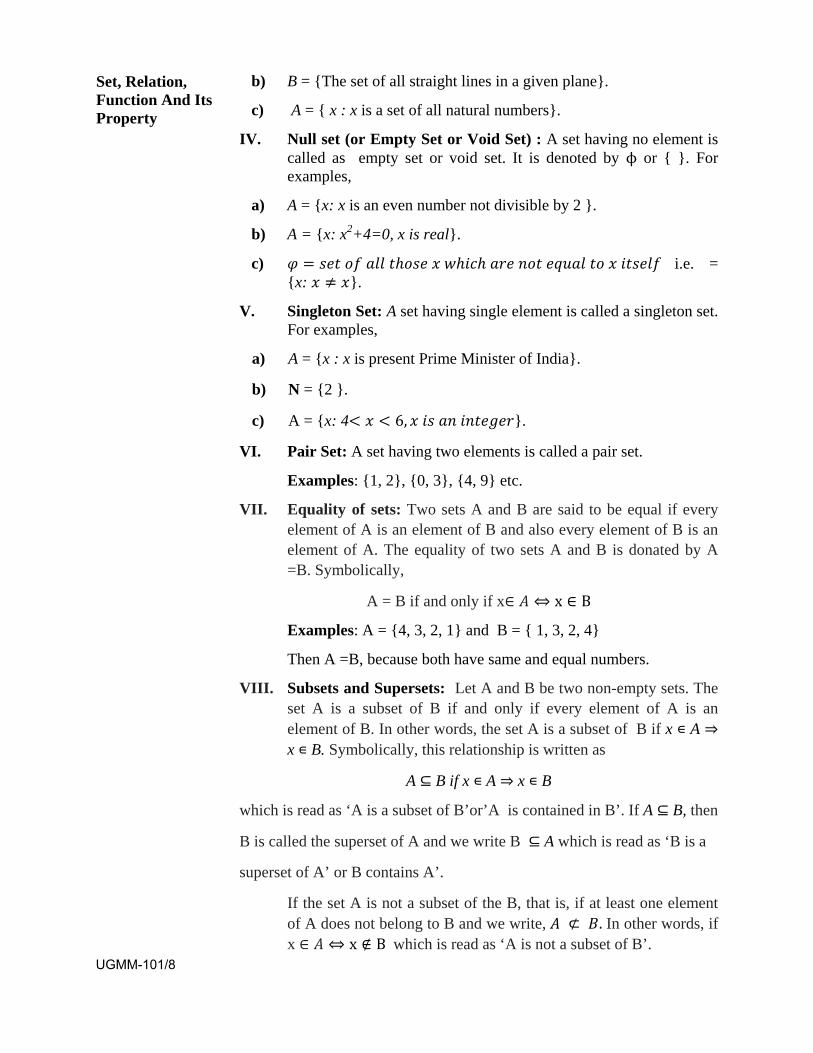


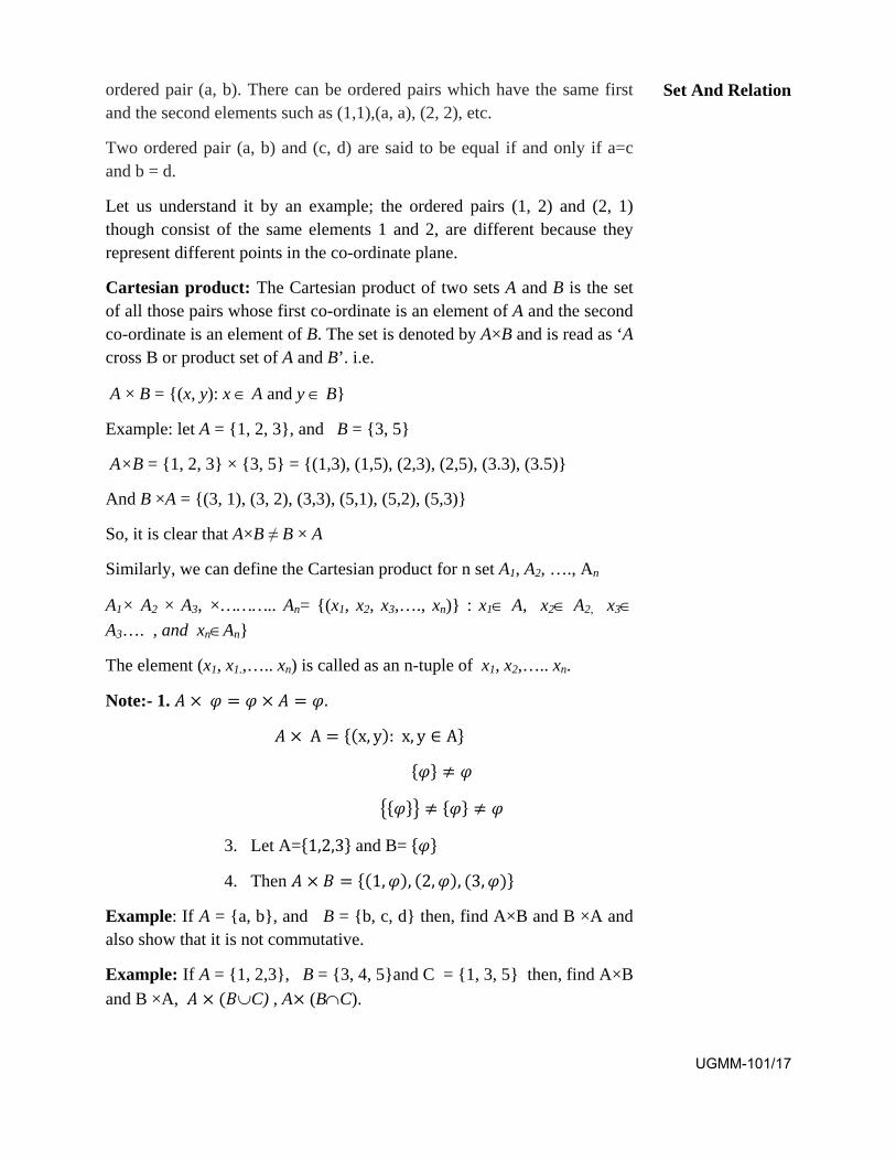


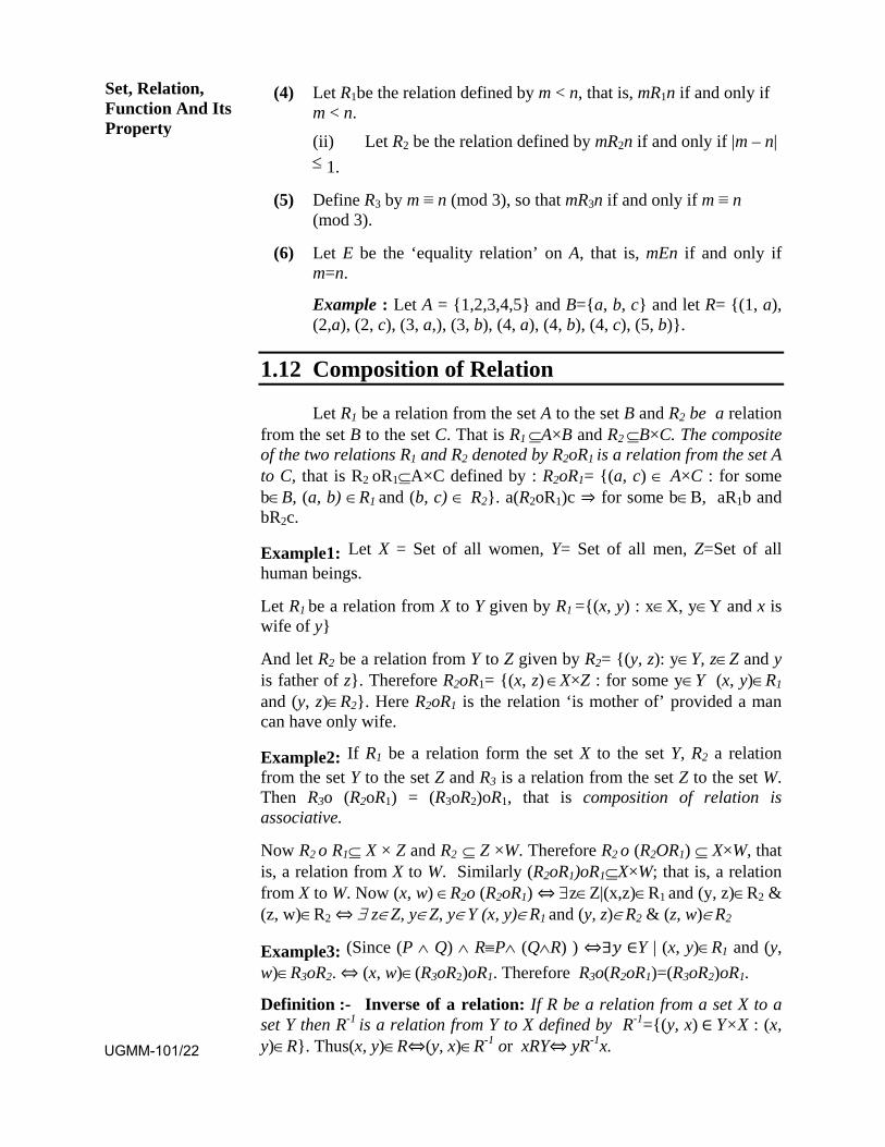


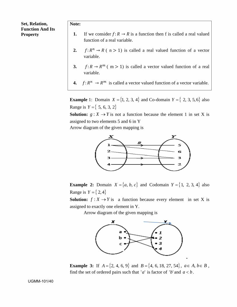
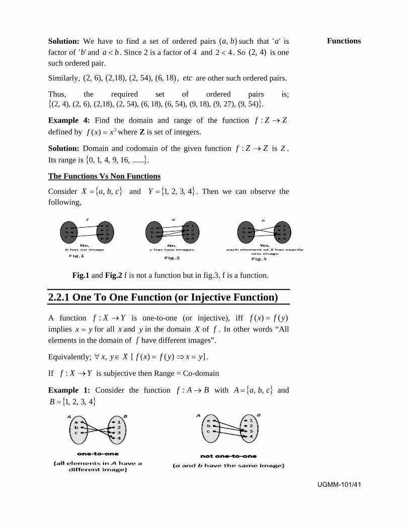


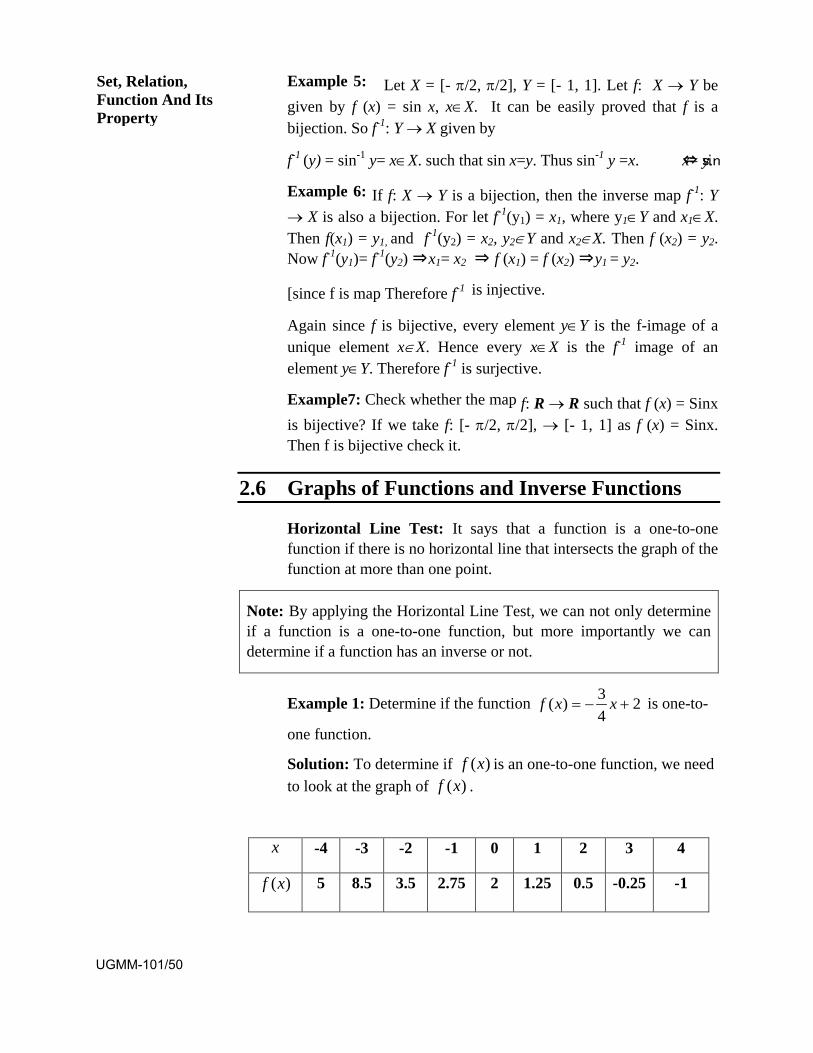


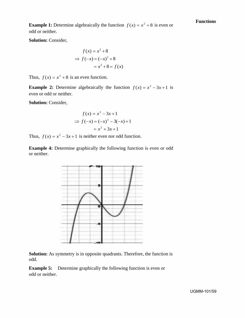


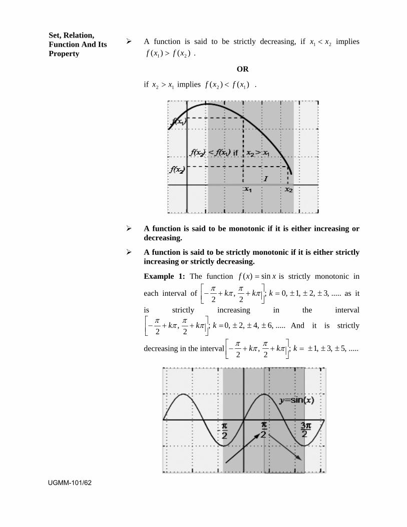
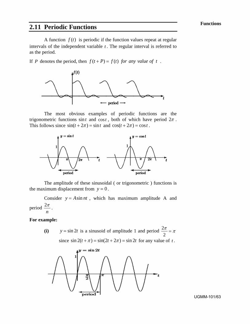


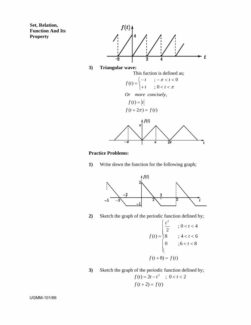

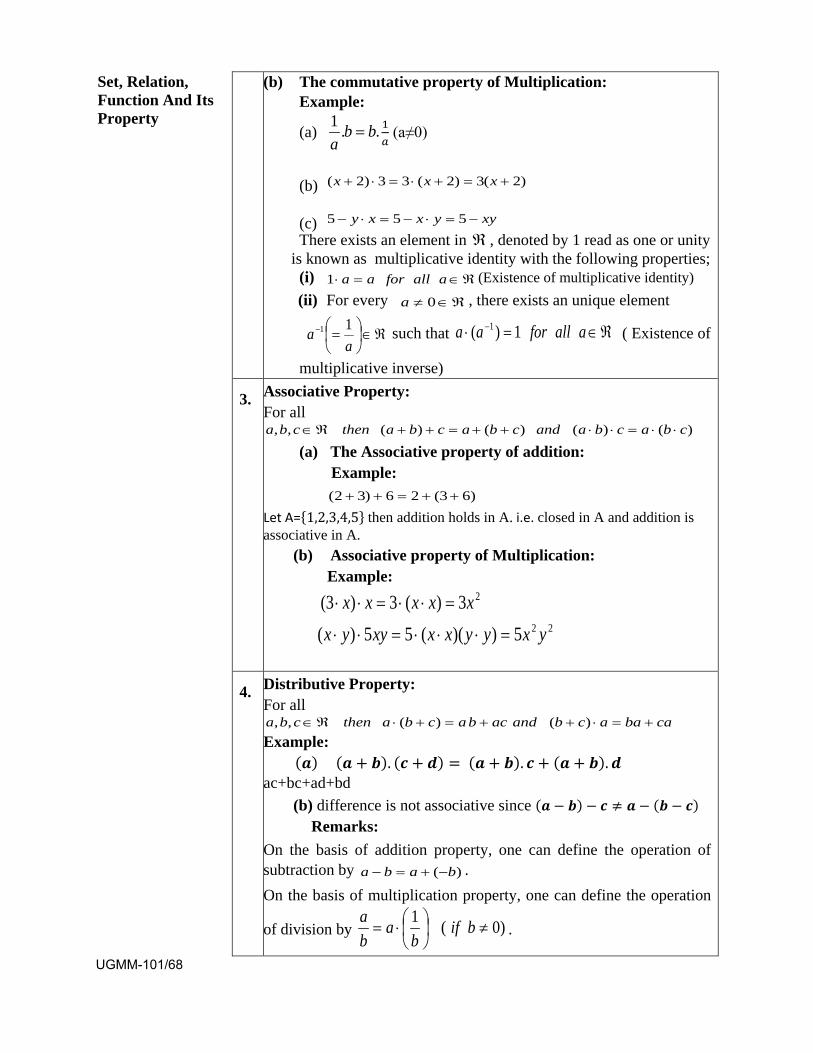


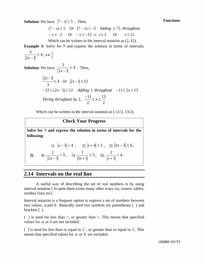


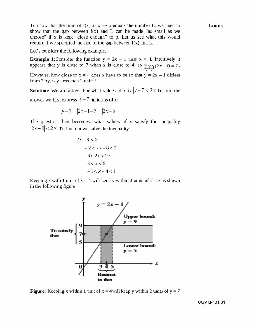


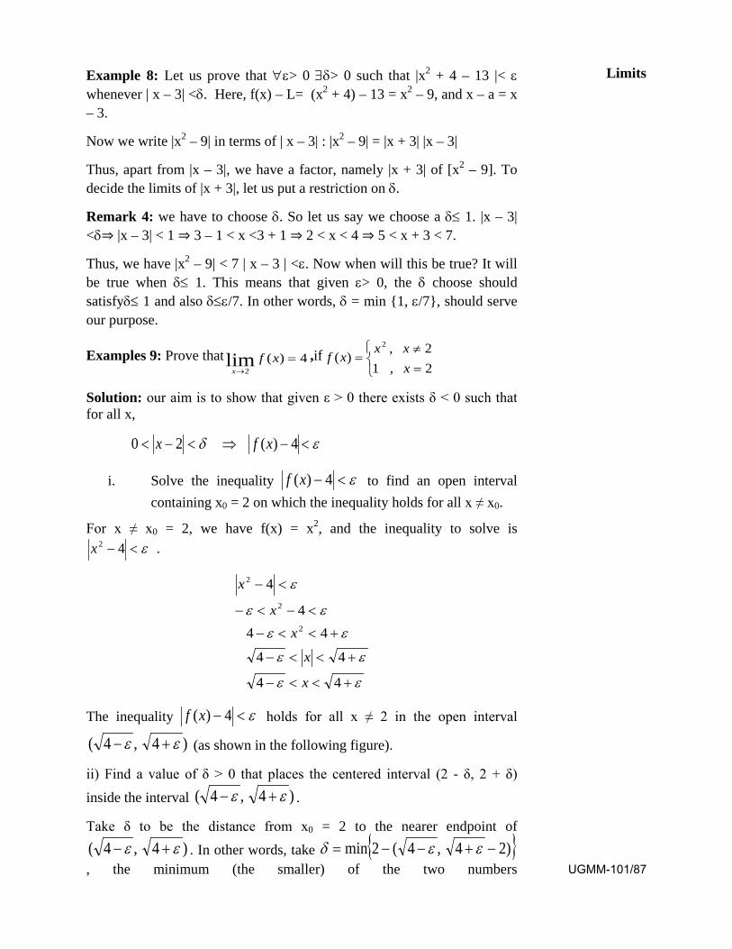
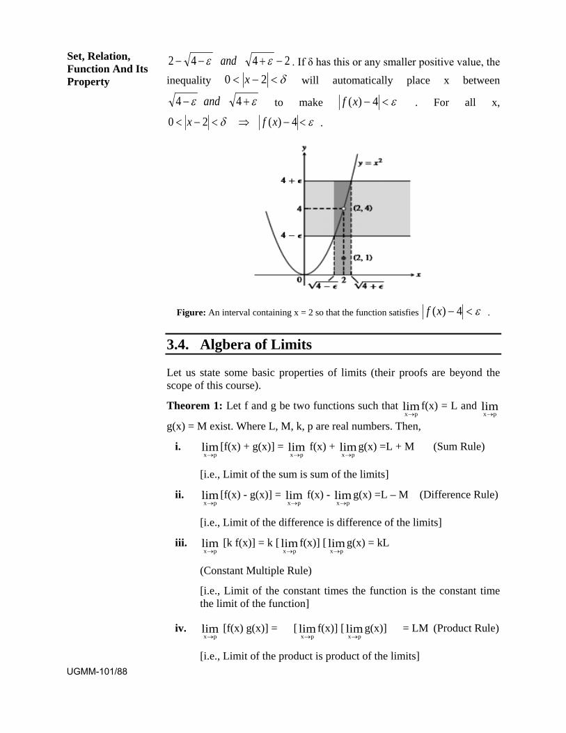


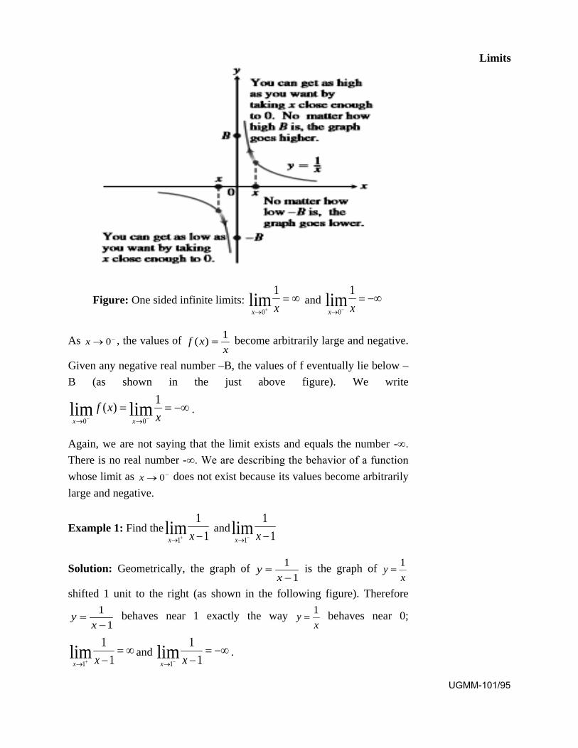


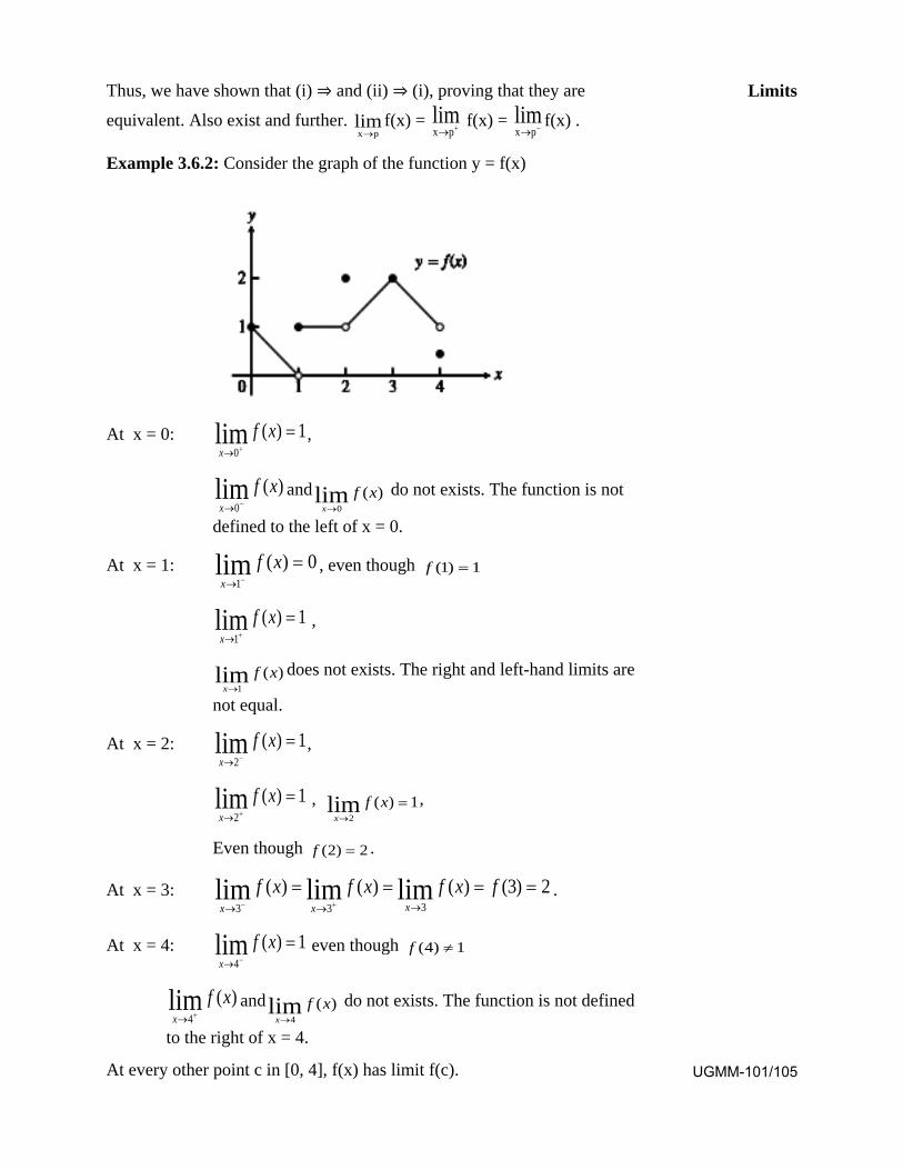


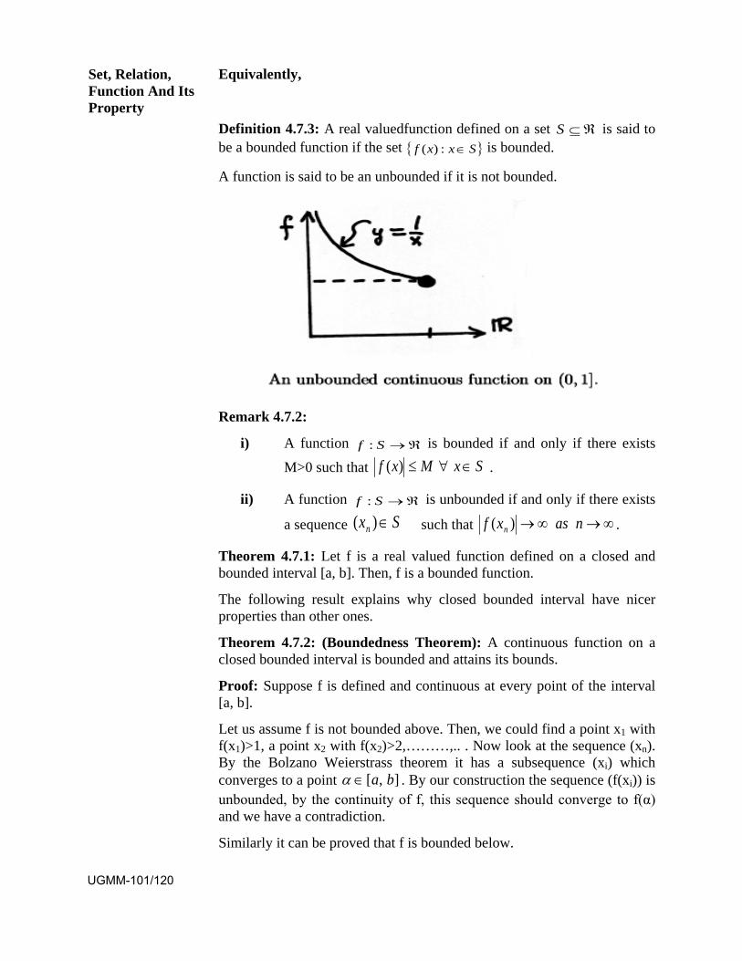

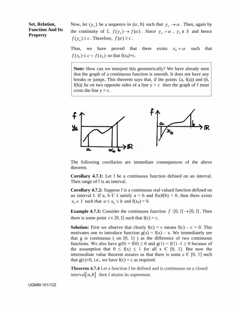


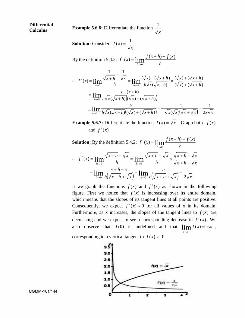


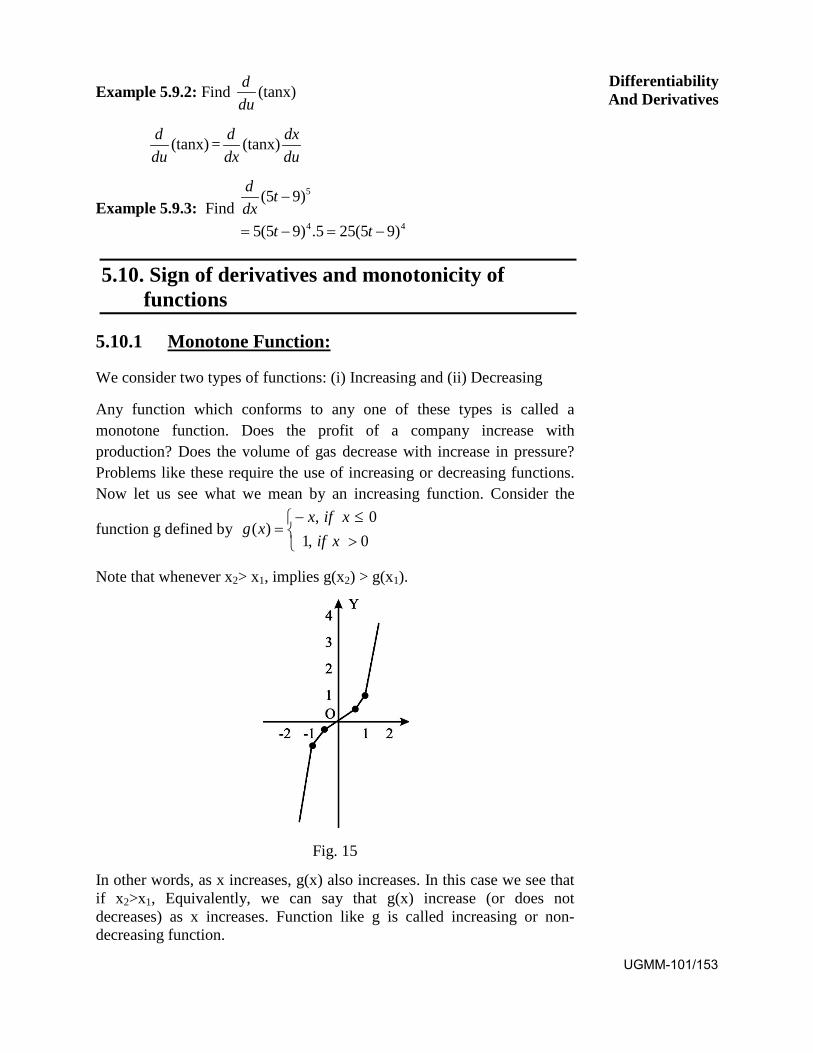


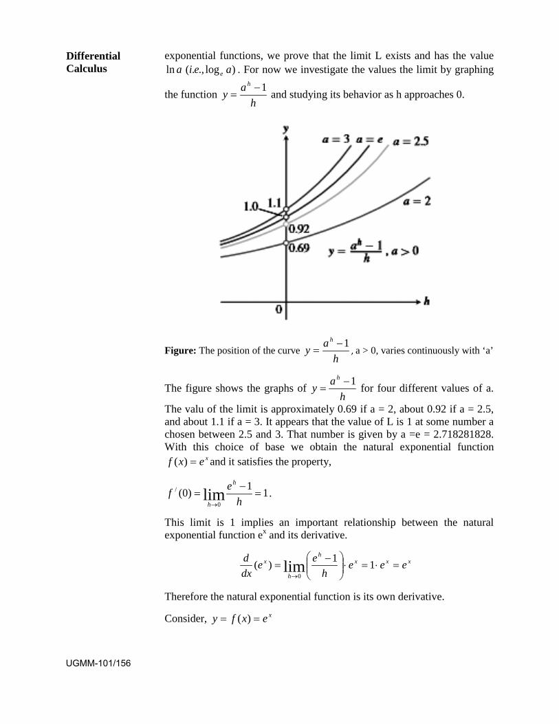
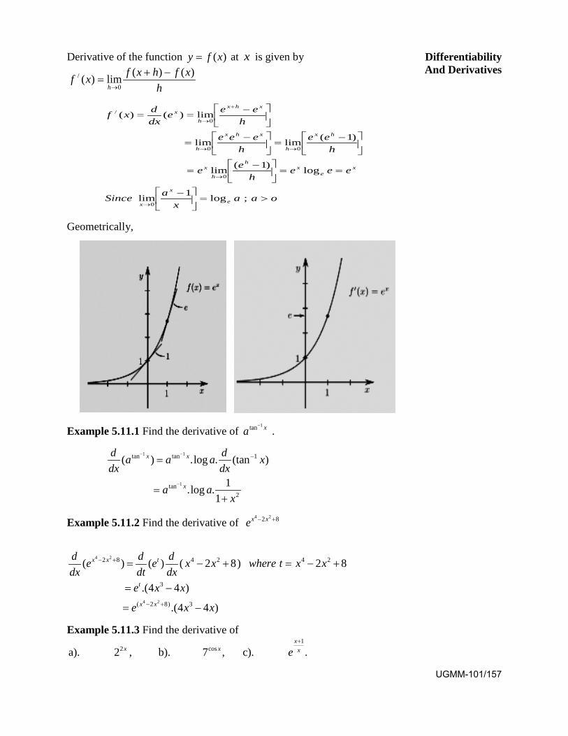


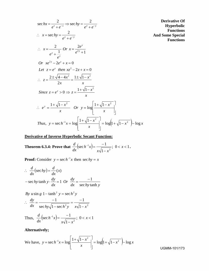

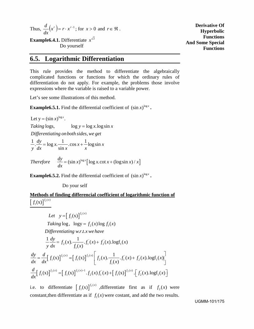
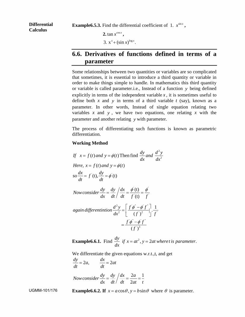


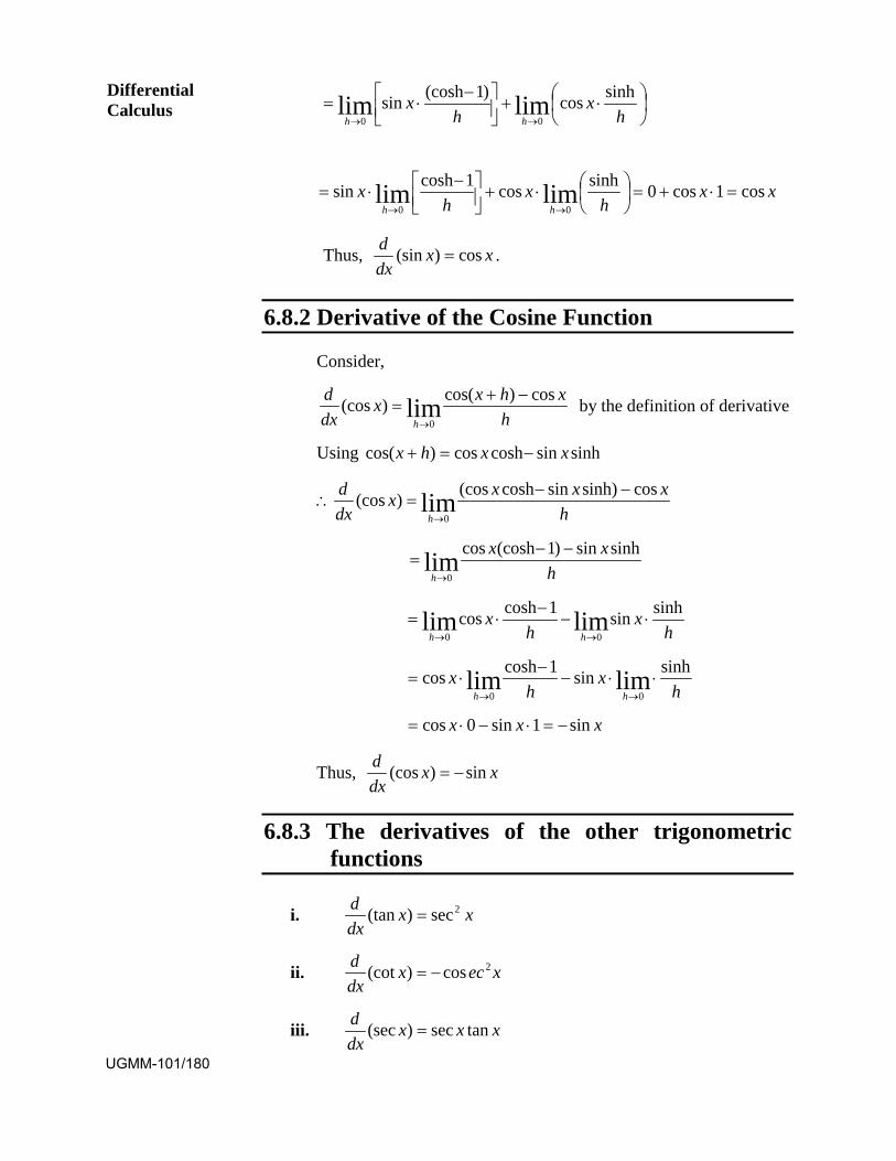
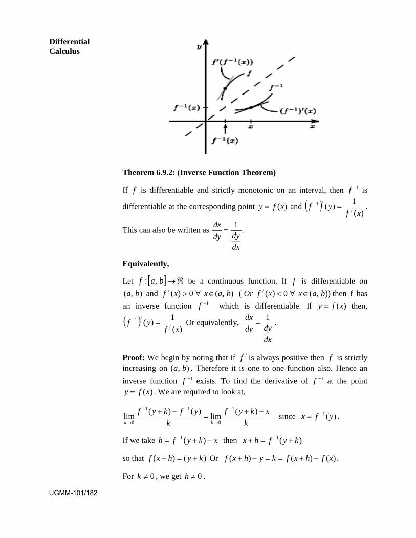
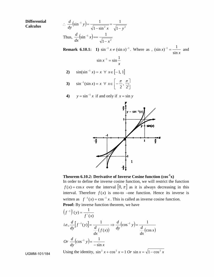
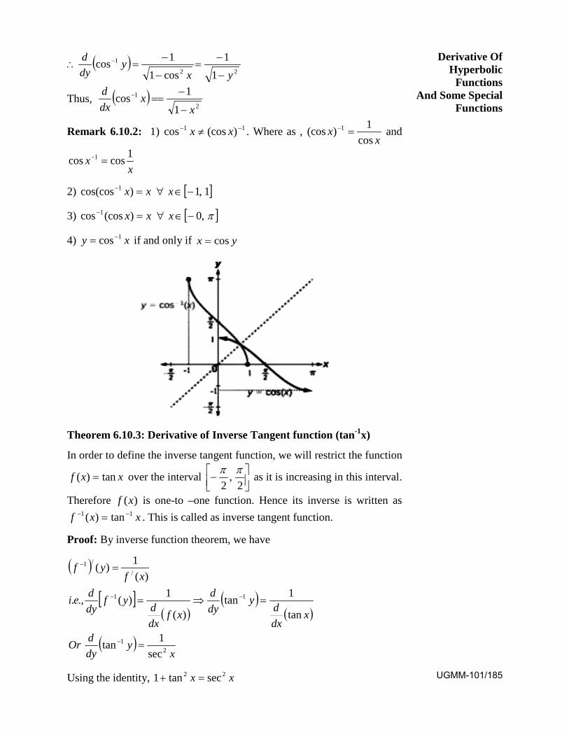


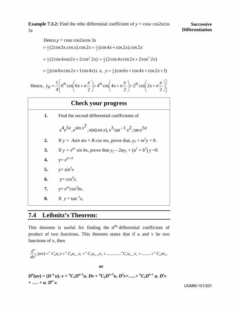


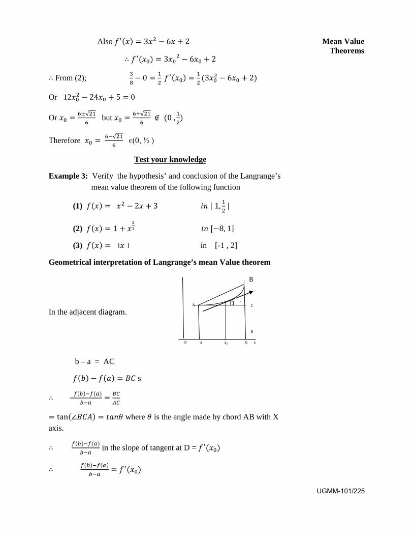


![Wimbledon AX3/5 BLOCK DIAGRAM 01 · Custom Block Diagram 1A Wednesday, November 25, 2009 130 Custom 3&% 67$&. 83 Wimbledon AX3/5 BLOCK DIAGRAM 01 / PAGE 29 RTL8103EL $]DOLD 5HDOWHN](https://static.documents.pub/doc/80x56/5e89ff4c3514a836a87544c8/wimbledon-ax35-block-diagram-01-custom-block-diagram-1a-wednesday-november-25.jpg)

