92
Bluelink Strategic Plan 2025

Bluelink Strategic Plan 2025


Strategic Plan 2025 Document Structure1. Goal2. Vision 3. Objectives 4. Scope 5. About the Partnership 6. Ocean Modelling 7. Bluelink Infrastructure 8. Bluelink Partnership Delivery Pathways 9. Governance Structure and Bluelink Documents 10. Communication and Stakeholder Engagement11. Risk Management
AnnexesA. Bluelink Collaborating Partners B. Bluelink Portfolio Roadmap C. Bluelink Management Committee Terms of
Reference D. Bluelink Operations and Development
Committee Terms of Reference E. Bluelink MSA-OSOFS KPIs

GoalDevelop and maintain world-leading global, regional, and littoral ocean forecast systems to support Defence applications and maintain a national ocean forecasting capability for Australia.

VisionBluelink capabilities are world-leading in prediction of the upper ocean in priority areas including the Indo-Pacific-Southern Ocean domain. Bluelink forecast systems deliver fit-for-purpose atmospheric, wave and ocean forecasts to the Department of Defence at global, regional, shelf and littoral-scales, including user-initiated forecasts.

Objectives1. Sustainment of world-leading global and high-resolution ocean-atmosphere-wave forecasts. 2. Enhance ocean forecasting capabilities through a portfolio of research and development activities. 3. Collaborate as strong partners in the ocean forecasting enterprise, to generate synergies from partner efforts and provide leadership for the benefit of Australia.

Annex A Bluelink Collaborating PartnersBesides the three Bluelink partners, there are crucial collaborating partners which are IMOS, DSTG, NCI, and the University sector. BoM and CSIRO’s extensive experience in the development and sustainment of ocean forecasting services is complimented by each of the Collaborating Partners, who deliver critical support to Bluelink partners.

Australia’s National Science Agency
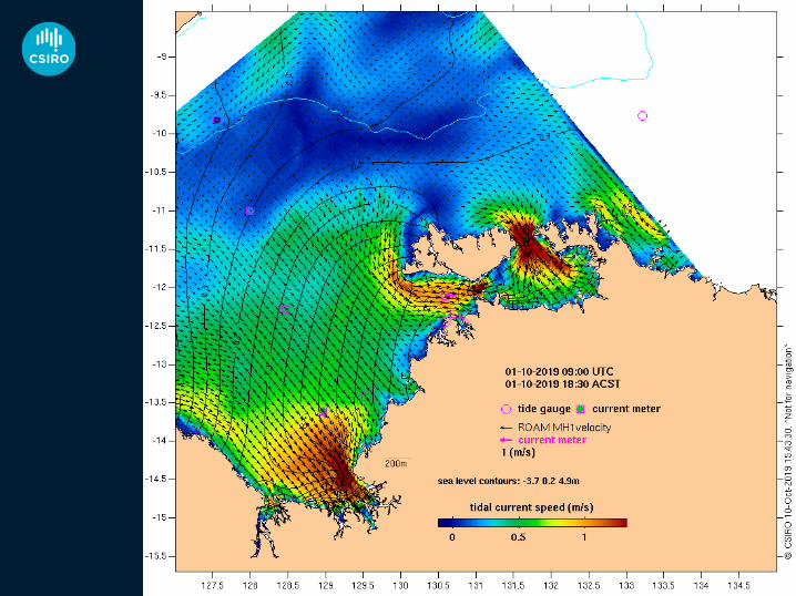
Bluelink regional-scale ocean modelling –basic test: barotropic tides
David Griffin (+many CSIRO colleagues)| 16 October 2019

• This is why IMOS (and other) in situ ocean observations are important to Bluelink, even if those obs are not used by the model• ROAM = Relocatable Ocean Atmosphere Model• Nested within OceanMAPS, adds tides. Hourly output. • But how credible is it? Would you make an operational
decision, with lives or $M at stake, based on it?
Advice is useless unless you know how credible it is

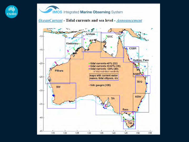
• And in many places, it is most of the variance• So why is there not an official tidal current prediction, but
only predictions of tidal sea level?• Because the credibility of tidal current predictions is either
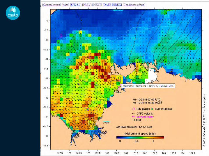
too low, unknown, or both.• OceanCurrent now has a tides section, presenting OTPS
predictions and comparison with 82 IMOS and other current meters. • Let’s start with Palm Passage, near Townsville.
The most predictable thing about the ocean is the tide.
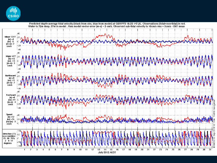


• For those regions where tides are dominant, useful predictions of currents can be made as far ahead as you like.• (not shown, but trust me) The next most predictable thing is
the response to wind, e.g. flooding in Adelaide. This is also predictable. But so are the energetic inertial oscillations.• The challenges: internal tides (NW especially, but elsewhere
too) and eddies/boundary currents.
Conclusions

Australia’s National Science Agency
CSIRO Oceans and AtmosphereDavid Griffin
+61 3 [email protected]
Thank you

Australia’s National Science Agency
AtRegional & Littoral
ScalesEdward King | 16/10/2019For: • Emlyn Jones & Uwe Rosebrock, and• Ron Hoeke, Paul Branson & Stephanie Contardo

How much information do you need to manage risk?
Imagine you are diving and this is the only piece of information you have to decide if it is safe.

How much information do you need to manage risk?
What about now?

How much information do you need to manage risk?
What about now?

How much information do you need to manage risk?
… or now?
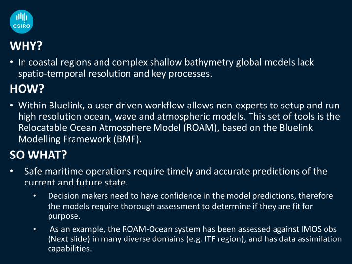
WHY?• In coastal regions and complex shallow bathymetry global models lack
spatio-temporal resolution and key processes.HOW?• Within Bluelink, a user driven workflow allows non-experts to setup and run
high resolution ocean, wave and atmospheric models. This set of tools is the Relocatable Ocean Atmosphere Model (ROAM), based on the BluelinkModelling Framework (BMF).
SO WHAT?• Safe maritime operations require timely and accurate predictions of the
current and future state.• Decision makers need to have confidence in the model predictions, therefore
the models require thorough assessment to determine if they are fit for purpose.
• As an example, the ROAM-Ocean system has been assessed against IMOS obs(Next slide) in many diverse domains (e.g. ITF region), and has data assimilation capabilities.

ROAM-Ocean: SST forecast error growth

ROAM-Ocean: Indonesian throughflow 1. T at Surface

ROAM-Ocean: Indonesian throughflow2. T at 100m

• 2003 - ‘What if we could allow a non-expert user to reliably run small-scale ocean and atmosphere models’• Originally conceived as desktop client for remote (and
dedicated) HPC
Bluelink Modelling Framework 1
Supports:• SHOC (Sparse Hydro Ocean Code), CSIRO• COMPAS (Coastal Ocean Marine
Prediction Across Scales , unstructured grids), CSIRO
• CCAM (Cubic Conformal Atmospheric Model), CSIRO
• SWAN wave mode, Deltares• XBEACH littoral zone model, Deltares• & several others (now obsolete) DSHPC
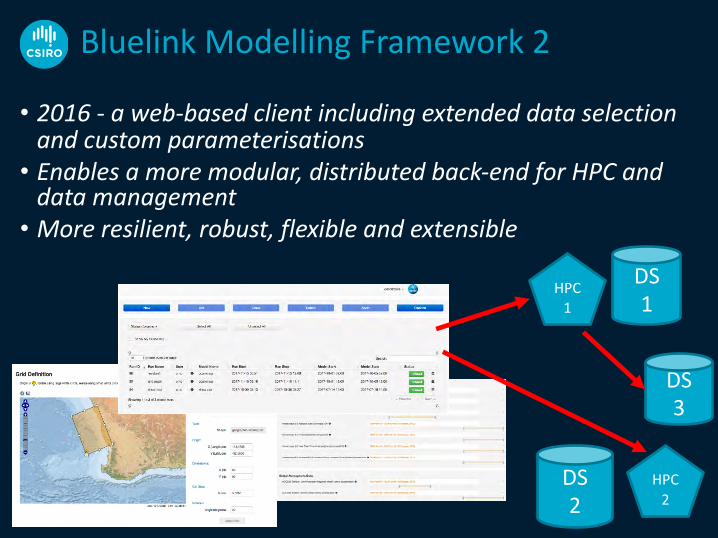
Bluelink Modelling Framework 2
• 2016 - a web-based client including extended data selection and custom parameterisations• Enables a more modular, distributed back-end for HPC and
data management• More resilient, robust, flexible and extensible
DS1
DS3
DS2
HPC1
HPC2

• Will be user-driven by client and scientific needs• Data flows
• Tighter and more seamless coupling between component models• New data streams for assimilation (Himawari-8 and SWOT)
• Underlying models• Taking advantage of new modelling technologies (e.g. unstructured grids – COMPAS and SWAN)• Compute architecture changes
• Ongoing deployment of field-based modelling capability• You don’t always have access to HPC infrastructure when in the field, but still need to make informed
decisions.• Data assimilation and automated model assessments
• Ongoing refinement of the DA methods to take advantage of observing system upgrades and new observational products.
• Real-time and automated assessment of model skill to alert decision makers if/when degraded performance is apparent.
BMF Strategic Development
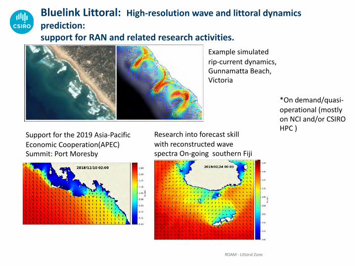
Research into forecast skill with reconstructed wave spectra On-going southern Fiji
Support for the 2019 Asia-Pacific Economic Cooperation(APEC) Summit: Port Moresby
*On demand/quasi-operational (mostly on NCI and/or CSIRO HPC )
Bluelink Littoral: High-resolution wave and littoral dynamics prediction:support for RAN and related research activities.
ROAM - Littoral Zone
Example simulated rip-current dynamics, Gunnamatta Beach, Victoria
Ron Hoeke, Paul Branson, Stephanie Contardo
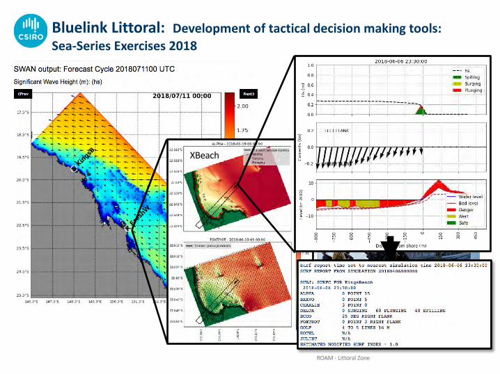
XBeach
ROAM - Littoral Zone
Bluelink Littoral: Development of tactical decision making tools:Sea-Series Exercises 2018
ROAM - Littoral Zone
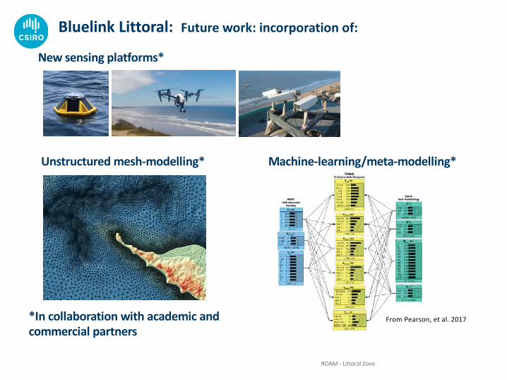
Bluelink Littoral: Future work: incorporation of:
New sensing platforms*
Unstructured mesh-modelling* Machine-learning/meta-modelling*
*In collaboration with academic and commercial partners
From Pearson, et al. 2017

Australia’s National Science Agency
Oceans & AtmosphereBluelink Lead: [email protected]
Regional Forecasting: [email protected]
Littoral Forecasting: [email protected]
Thank you

Operational ocean forecasting @ BoMoperational since 2007
Brassington, Entel, Zhong, Sakov, Divakaran, Beggs, Huang, Sweeney, Velic, Freeman, Beckett

Overview
Global ocean forecasting system statussee talk Sweeney AMOS-2019see poster Brassington OceanPredict’19 see talk Divakaran, Bluelink science workshop
Next generation global ocean forecastingsee talk Sakov, Bluelink science workshopsee talk Kiss, AMOS-2019see talk Brassington, OceanPredict’19
Next generation regional ocean forecastingsee talk Brassington AMOS-2019
0
0.5
1
1.5
2

Ocean Model Analysis and Prediction System OceanMAPS version 3.2
Ocean ModelMOM 5z* vertical coordinateSmith and Sandwell, v11.13599×1499×51
0-360, 75S-75N (0.1°×0.1°)0-15 m (Δz = 5 m)15-90 m (Δz~5 to 10 m)90-200m (Δz=10 m)Minimum column depth – 15 m
GOTM, K-eps mixed layer schemeNo tidesNo sea-ice
Data AssimilationENKF-C (Sakov, 2014)Ensemble optimal interpolationState vector (eta, T, S, u, v)144-member ensemble Restart initialisation
Observations Satellite altimetry (Jason3, Sentinel3A, Cryosat2, AltiKa) Satellite SST (Metop-A, Metop-B, VIIRS, AVHRR, AMSR2)In situ profiles Argo, CTD, XBT
ForcingACCESS-G APS2 (fluxes)Climatological river discharge
Thanks also to GFDL, the global ocean observing system, IMOS and JCOMM

1st$$$$$2nd$$$$3rd$$$$4th$$$$5th$$$$6th$$$$7th$$$$8th$$$$9th$$$10th$$11th$$12th$$13th$$14th$$15th$$16th$$17th$$18th$$19th$$20th$$21st$$22nd$23rd$$$�
9th�
10th�
11th�
12th�
13th�
$$14th�
15th�
16th�
Date$of$e
xecu:o
n�
BRT hindcast!
NRT and BRT!use a common !
background !
;144h$;120h$$;96h$$$;72h$$$;48h$$$$;24h$$$$$$0$$$$$$$24h$$$$$48h$$$$72h$$$$$96h$$$120h$$144h�
3-cycle mean�
Valid$date$for$the$hindcast$and$forecast$�
Forecast cycle�
NRT !hindcast! Forecast!
BRT assimilation!
NRT 24hr initialisation!
BRT 24hr initialisation!
NRT assimilation!
Forecast$hour�+/;$1.5$days$Al:metry$Profiles$SST$
+/;$1.5$days$Al:metry$Profiles$SST$
Sea surface temperature ensemble STDJan 2013
Sea surface temperature ensemble STD (degC)
0.0 0.1 0.2 0.3 0.4 0.5 0.6 0.7 0.8 0.9 1.0Data Min = 0.0, Max = 5.7
0.1
0.1
0.1
0.20.2
0.2
0.2
0.2
0.2
0.2
0.2
0.2
0.20.2
0.2
0.20.2
0.2
0.2
0.2
0.2
0.2 0.2
0.3 0.3 0.3
0.3
0.3
0.3
0.30.3
0.3
0.3
0.3
0.3
0.3
0.3
0.3
0.4
0.4 0.40.4 0.
4
0.4
0.40.
4
0.4
0.4
0.5
0.5
0.5
0.5
0.6
0.60.6
0.7
0.7
0.7
34S
36S
38S
40S
42S
144E 146E 148E 150E 152E 154E 156E 158E 160E 162E 164E 166E
Sea surface temperature ensemble meanJan 2013
Sea surface temperature ensemble mean (degC)
13.0 14.0 15.0 16.0 17.0 18.0 19.0 20.0 21.0 22.0 23.0 24.0 25.0 26.0 27.0Data Min = -1.1, Max = 40.1
15.0 15.0
15.0
16.0
16.0
16.0
17.0
17.0
17.0
18.0
18.0
19.020.0
21.0
22.0
23.0
24.0
25.0
34S
36S
38S
40S
42S
144E 146E 148E 150E 152E 154E 156E 158E 160E 162E 164E 166E
Jan 2013Jan 2013
Sea surface temperature ensemble meanJan 2012
Sea surface temperature ensemble mean (degC)
13.0 14.0 15.0 16.0 17.0 18.0 19.0 20.0 21.0 22.0 23.0 24.0 25.0 26.0 27.0Data Min = -1.1, Max = 39.6
15.0 15.016.0
16.0
16.0
17.0 17.0
17.0
18.0
18.0
19.0
19.0
19.0
20.0
21.0
22.0
22.0
23.0
24.0
34S
36S
38S
40S
42S
144E 146E 148E 150E 152E 154E 156E 158E 160E 162E 164E 166E
SST monthly average ensemble mean SST monthly average ensemble STD
Sea surface temperature ensemble STDJan 2013
Sea surface temperature ensemble STD (degC)
0.0 0.1 0.2 0.3 0.4 0.5 0.6 0.7 0.8 0.9 1.0Data Min = 0.0, Max = 5.7
0.1
0.1
0.1
0.20.2
0.2
0.2
0.2
0.2
0.2
0.2
0.2
0.20.2
0.2
0.20.2
0.2
0.2
0.2
0.2
0.2 0.2
0.3 0.3 0.3
0.3
0.3
0.3
0.30.3
0.3
0.3
0.3
0.3
0.3
0.3
0.3
0.4
0.4 0.40.4 0.
4
0.4
0.4
0.4
0.4
0.4
0.5
0.5
0.50.5
0.6
0.60.6
0.7
0.7
0.7
34S
36S
38S
40S
42S
144E 146E 148E 150E 152E 154E 156E 158E 160E 162E 164E 166E
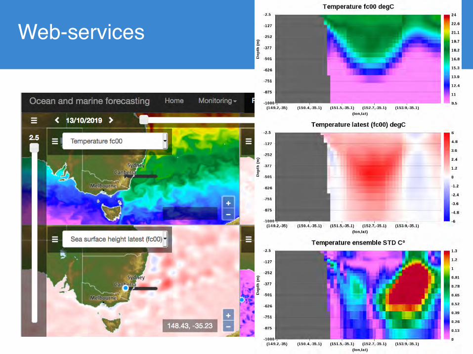
Web-services

Intercomparison – Argo (2018)Day 1 forecast
Mean Absolute Difference
-Australia - UK - France - Canada
Tem
pera
ture
Salin
ity
Mean Difference
Australian region
Global baseline performanceTemperature comparable MD/MAD Salinity outlier in MD

TCcold-core
eddy
•Hot water everywhere 18th
March 2019
•Along comes TC Veronica …
EarthData NASA
CASE STUDY 3
see Sweeney, AMOS 2019 talk

144 hrs 120 hrs
96 hrs 72 hrs
48 hrs 24 hrs
Forecasts for 24th
March 2019 by lead time
0 hrs
TCcold-core
eddy
Was it forecasted?

4-hour SST an –25th 00z
6-day SST an – centred 25th 00z
IMOS Ocean Current
Model 24-hr avg – centred 25th 00z
The cloud cleared on the 24th …
TCcold-core
eddy

Unusual cold-core
eddy
1st percentile exceedence
Temp at 48 m
SLA
• Extreme cold eddy south of Java
• Temps over 6 deg cooler than 1st
percentile
CASE STUDY 4

NOAA: YouTube
RAN dropped XBTs5th Dec 2018
Temp at 105 m
Comparison with XBTs
Unusual cold-core
eddy

Ocean Model Analysis and Prediction System OceanMAPS version 3.3 – TARGET 2018
Ocean ModelMOM 5.1z* vertical coordinateSmith and Sandwell, v11.13599×1499×50
0-360, 75S-75N (0.1°×0.1°)0-15 m (Δz = 5 m)15-90 m (Δz~5 to 10 m)90-200m (Δz=10 m)Minimum column depth – 15 m
GOTM, K-epsNo tidesNo sea-ice
Data AssimilationENKF-C (Sakov, 2014)Ensemble optimal interpolationState vector (eta, T, S, u, v)144-member ensemble Restart initialisation
ObservationsSatellite altimetry (Jason3, Sentinel3A, Cryosat2, AltiKa) Satellite SST (Metop-A, Metop-B, VIIRS, AVHRR, AMSR2)In situ profiles Argo, CTD, XBT
ForcingACCESS-G APS3 (bulk-formulae)Climatological river discharge
Thanks also to GFDL, the global ocean observing system, IMOS and JCOMM

SST Data Assimilation stats
see Divakaran

OceanMAPS v3.x
SkilfulFirst glimpse at forecast uncertaintyOutperforming BRANInternationally competitiveRobust and up to dateCapable of capturing synoptic anomalous conditions
Highly recommended for downscaling
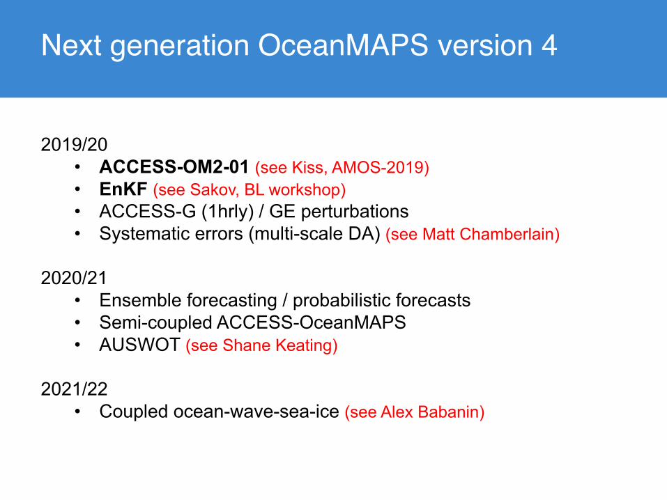
Next generation OceanMAPS version 4
2019/20• ACCESS-OM2-01 (see Kiss, AMOS-2019)• EnKF (see Sakov, BL workshop)• ACCESS-G (1hrly) / GE perturbations• Systematic errors (multi-scale DA) (see Matt Chamberlain)
2020/21• Ensemble forecasting / probabilistic forecasts• Semi-coupled ACCESS-OceanMAPS• AUSWOT (see Shane Keating)
2021/22• Coupled ocean-wave-sea-ice (see Alex Babanin)

ACCESS-OM2-01
Kiss, Hogg,Spence, England,
Heil, Oke,Brassington,
Hannah, Fiedler,Heerdegen, Ward
The ACCESS-OM2 model suiteACCESS-OM2 is being developed by COSIMA (cosima.org.au)
I Ocean model: Modular Ocean Model (MOM) 5.1I global (90�N – 81�S); tripolar in Arctic; Mercator for 65�N – 65�SI three resolutions: 1�, 0.25�, 0.1� horizontal resolutionI z⇤ vertical coordinate, 50 or 75 levelsI Initial condition and salt restoring: World Ocean Atlas 2013v2
I Sea-ice model: CICE 5.1I classic EVP dynamics (for now)I ridging scheme with 5 thickness categoriesI mushy ice thermodynamics at 0.1� (for now), 4 ice layers + 1 snow
I Prescribed atmospheric forcing: JRA55-doI Coupler: OASIS3-MCTI End-users:
I for nationwide use in ocean and sea ice process studiesI to form the dynamical core of Bluelink (OceanMAPSv4.0), to extend Bluelink
reanalyses and forecasts to global coverage, including sea iceI to inform the development of higher-resolution future versions of the ACCESS
coupled climate model
ACCESS-OM2-01
Kiss, Hogg,Spence, England,
Heil, Oke,Brassington,
Hannah, Fiedler,Heerdegen, Ward
ACCESS-OM2-01,
a global 0.1-degree
ocean-sea ice modelfor the next phase of Bluelink
Andrew Kiss ([email protected]),Andy Hogg (ANU), Paul Spence (UNSW), Matthew England (UNSW),
Petra Heil (AAD & ACE CRC, UTas), Peter Oke (CSIRO),Gary Brassington (BOM), Nicholas Hannah (Double Precision),
Russell Fiedler (CSIRO), Aidan Heerdegen (ANU), Marshall Ward (ANU),
December 4, 2018
Next generation OceanMAPS v4.0 (model)
cosima.org.auCOSIMA
Herding theAustralian ocean
modellingcommunity
to work together
Kiss, Hogg,Spence, England,
Heil, Oke,Brassington,Nikurashin,
Hannah, Fiedler,Heerdegen,Munroe, Wu,
Stewart, Morrison,Ward, Freeman
COSIMA andACCESS-OM2
Progress
Results
Future
Vertical resolution
�z=1.1 – 198m (cf. 5 – 1000m in OFAM3)75 level vertical grid is finer than OFAM3 at all depths other than 100 – 260mSpacing optimised for resolving baroclinic modes
Relative error in baroclinic modesGrid E (R1) E (R2) E (R3)KDS75 0.346 0.384 0.408OFAM51 0.490 0.542 0.562
(Stewart et al., 2017)
Stewart et al., (2017)

ACCESS-OM2-01
Kiss, Hogg,Spence, England,
Heil, Oke,Brassington,
Hannah, Fiedler,Heerdegen, Ward
The ACCESS-OM2 model suiteACCESS-OM2 is being developed by COSIMA (cosima.org.au)
I Ocean model: Modular Ocean Model (MOM) 5.1I global (90�N – 81�S); tripolar in Arctic; Mercator for 65�N – 65�SI three resolutions: 1�, 0.25�, 0.1� horizontal resolutionI z⇤ vertical coordinate, 50 or 75 levelsI Initial condition and salt restoring: World Ocean Atlas 2013v2
I Sea-ice model: CICE 5.1I classic EVP dynamics (for now)I ridging scheme with 5 thickness categoriesI mushy ice thermodynamics at 0.1� (for now), 4 ice layers + 1 snow
I Prescribed atmospheric forcing: JRA55-doI Coupler: OASIS3-MCTI End-users:
I for nationwide use in ocean and sea ice process studiesI to form the dynamical core of Bluelink (OceanMAPSv4.0), to extend Bluelink
reanalyses and forecasts to global coverage, including sea iceI to inform the development of higher-resolution future versions of the ACCESS
coupled climate model
ACCESS-OM2-01
Kiss, Hogg,Spence, England,
Heil, Oke,Brassington,
Hannah, Fiedler,Heerdegen, Ward
ACCESS-OM2-01,
a global 0.1-degree
ocean-sea ice modelfor the next phase of Bluelink
Andrew Kiss ([email protected]),Andy Hogg (ANU), Paul Spence (UNSW), Matthew England (UNSW),
Petra Heil (AAD & ACE CRC, UTas), Peter Oke (CSIRO),Gary Brassington (BOM), Nicholas Hannah (Double Precision),
Russell Fiedler (CSIRO), Aidan Heerdegen (ANU), Marshall Ward (ANU),
December 4, 2018
Next generation OceanMAPS v4.0 (model)
Expected benefits
Defence: Afternoon effect, Mixed layer, ThermoclineMaritime Safety: 1.1m (top cell), hrly, Mixed layer currents, Sea-ice concentration etc.Coastal operations: Improved surge/upwelling, CTW’sWeather forecasting: Full global SST and sea-ice concentration forecastsDownscaling: Reduced systematic biases

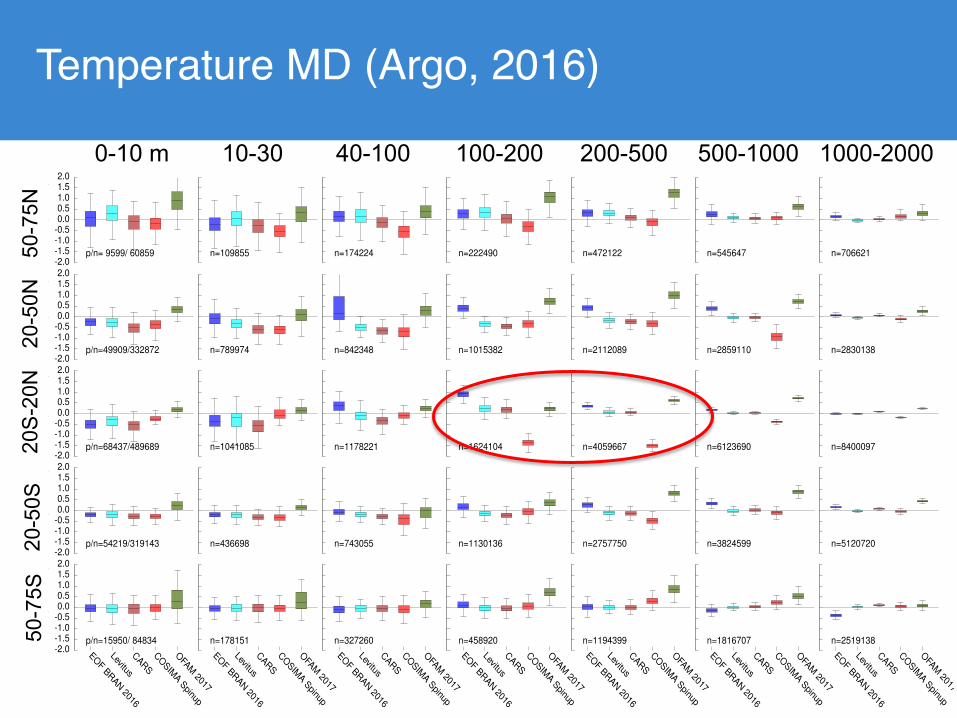
Temperature MD (Argo, 2016)
Temperature Bias compared to observations (2016)
-2.0
-1.5
-1.0
-0.5
0.0
0.5
1.0
1.5
2.0
p/n= 9599/ 60859 n=109855 n=174224 n=222490 n=472122 n=545647 n=706621
-2.0
-1.5
-1.0
-0.5
0.0
0.5
1.0
1.5
2.0
p/n=49909/332872 n=789974 n=842348 n=1015382 n=2112089 n=2859110 n=2830138
-2.0
-1.5
-1.0
-0.5
0.0
0.5
1.0
1.5
2.0
p/n=68437/489689 n=1041085 n=1178221 n=1624104 n=4059667 n=6123690 n=8400097
-2.0
-1.5
-1.0
-0.5
0.0
0.5
1.0
1.5
2.0
p/n=54219/319143 n=436698 n=743055 n=1130136 n=2757750 n=3824599 n=5120720
-2.0
-1.5
-1.0
-0.5
0.0
0.5
1.0
1.5
2.0
EOF
BRAN
2016
Levitu
s
CARS
COSIM
ASpinup
OFAM
2017
p/n=15950/ 84834
EOF
BRAN
2016
Levitu
s
CARS
COSIM
ASpinup
OFAM
2017
n=178151
EOF
BRAN
2016
Levitu
s
CARS
COSIM
ASpinup
OFAM
2017
n=327260
EOF
BRAN
2016
Levitu
s
CARS
COSIM
ASpinup
OFAM
2017
n=458920
EOF
BRAN
2016
Levitu
s
CARS
COSIM
ASpinup
OFAM
2017
n=1194399
EOF
BRAN
2016
Levitu
s
CARS
COSIM
ASpinup
OFAM
2017
n=1816707
EOF
BRAN
2016
Levitu
s
CARS
COSIM
ASpinup
OFAM
2017
n=2519138
latitu
de
(50�
75)
Depth (0 � 10) m Depth (10 � 40) m Depth (40 � 100) m Depth (100 � 200) m Depth (200 � 500) m Depth (500 � 1000) m Depth (1000 � 2000) m
latitu
de
(20�
50)
Tem
pera
ture
Bia
s/� C
latitu
de
(-20�
20)
latitu
de
(-50�
-20)
latitu
de
(-75�
-50)
Temperature Bias compared to observations (2016)
-2.0
-1.5
-1.0
-0.5
0.0
0.5
1.0
1.5
2.0
p/n= 9599/ 60859 n=109855 n=174224 n=222490 n=472122 n=545647 n=706621
-2.0
-1.5
-1.0
-0.5
0.0
0.5
1.0
1.5
2.0
p/n=49909/332872 n=789974 n=842348 n=1015382 n=2112089 n=2859110 n=2830138
-2.0
-1.5
-1.0
-0.5
0.0
0.5
1.0
1.5
2.0
p/n=68437/489689 n=1041085 n=1178221 n=1624104 n=4059667 n=6123690 n=8400097
-2.0
-1.5
-1.0
-0.5
0.0
0.5
1.0
1.5
2.0
p/n=54219/319143 n=436698 n=743055 n=1130136 n=2757750 n=3824599 n=5120720
-2.0
-1.5
-1.0
-0.5
0.0
0.5
1.0
1.5
2.0
EOF
BRAN
2016
Levitu
s
CARS
COSIM
ASpinup
OFAM
2017
p/n=15950/ 84834
EOF
BRAN
2016
Levitu
s
CARS
COSIM
ASpinup
OFAM
2017
n=178151
EOF
BRAN
2016
Levitu
s
CARS
COSIM
ASpinup
OFAM
2017
n=327260
EOF
BRAN
2016
Levitu
s
CARS
COSIM
ASpinup
OFAM
2017
n=458920
EOF
BRAN
2016
Levitu
s
CARS
COSIM
ASpinup
OFAM
2017
n=1194399
EOF
BRAN
2016
Levitu
s
CARS
COSIM
ASpinup
OFAM
2017
n=1816707
EOF
BRAN
2016
Levitu
s
CARS
COSIM
ASpinup
OFAM
2017
n=2519138
latitu
de
(50�
75)
Depth (0 � 10) m Depth (10 � 40) m Depth (40 � 100) m Depth (100 � 200) m Depth (200 � 500) m Depth (500 � 1000) m Depth (1000 � 2000) m
latitu
de
(20�
50
)
Te
mp
era
ture
Bia
s/� C
latitu
de
(-2
0�
20
)la
titu
de
(-50�
-20
)la
titu
de
(-75�
-50)
Temperature MD (Argo, 2016)Temperature Bias compared to observations (2016)
-2.0
-1.5
-1.0
-0.5
0.0
0.5
1.0
1.5
2.0
p/n= 9599/ 60859 n=109855 n=174224 n=222490 n=472122 n=545647 n=706621
-2.0
-1.5
-1.0
-0.5
0.0
0.5
1.0
1.5
2.0
p/n=49909/332872 n=789974 n=842348 n=1015382 n=2112089 n=2859110 n=2830138
-2.0
-1.5
-1.0
-0.5
0.0
0.5
1.0
1.5
2.0
p/n=68437/489689 n=1041085 n=1178221 n=1624104 n=4059667 n=6123690 n=8400097
-2.0
-1.5
-1.0
-0.5
0.0
0.5
1.0
1.5
2.0
p/n=54219/319143 n=436698 n=743055 n=1130136 n=2757750 n=3824599 n=5120720
-2.0
-1.5
-1.0
-0.5
0.0
0.5
1.0
1.5
2.0
EOF
BRAN
2016
Levitu
s
CARS
COSIM
ASpinup
OFAM
2017
p/n=15950/ 84834
EOF
BRAN
2016
Levitu
s
CARS
COSIM
ASpinup
OFAM
2017
n=178151
EOF
BRAN
2016
Levitu
s
CARS
COSIM
ASpinup
OFAM
2017
n=327260
EOF
BRAN
2016
Levitu
s
CARS
COSIM
ASpinup
OFAM
2017
n=458920
EOF
BRAN
2016
Levitu
s
CARS
COSIM
ASpinup
OFAM
2017
n=1194399
EOF
BRAN
2016
Levitu
s
CARS
COSIM
ASpinup
OFAM
2017
n=1816707
EOF
BRAN
2016
Levitu
s
CARS
COSIM
ASpinup
OFAM
2017
n=2519138
latitu
de
(50�
75
)
Depth (0 � 10) m Depth (10 � 40) m Depth (40 � 100) m Depth (100 � 200) m Depth (200 � 500) m Depth (500 � 1000) m Depth (1000 � 2000) m
latitu
de
(20�
50
)
Te
mp
era
ture
Bia
s/� C
latitu
de
(-2
0�
20
)la
titu
de
(-5
0�
-20
)la
titu
de
(-7
5�
-50
)
0-10 m 10-30 40-100 1000-2000500-1000200-500100-200
50-7
5N20
-50N
20S-
20N
20-5
0S50
-75S

2019
EnKF2001
2012
1997
2008
EnOI
BenefitsEnKF more dynamically balanced / reduced smoothingBetter samples unlikely/extreme events
mesoscale eddies, boundary current meandersTC mixingUpwelling…
Ensemble (probabilistic) forecasting
Why move from EnOI to EnKF ?

Why not move from EnOI to EnKF ?
OFAM3 + EnKF-C • 96-member ensemble• RADS altimetry, NAVO, VIIRS, profiles • 3 day cycle• Localisation: 150 km SLA and SST
• 450 km T and S• 3% capped inflation• SST bias correction
Observation/model timing
model
observations
interval id
model
observations
previousanalysis analysis
−12 −11 −10 −9 −8 −7 −6 −5 −4 −3 −2 −1
model
interval id
observations
SST
SLA
T, S
0:00 12:00 0:00 12:00 0:00 12:00 0:00 12:00 0:00 12:00 0:00UTC time
9:0015:00 21:00 15:00 21:00 15:00 21:00 15:00 21:00 3:00 15:00 21:003:00 9:00 3:00 9:00 3:00 9:00 3:00 9:00
−2 −1 0
5 / 29
Resources:• CPU: ~9 kSU / cycle• Footprint: 4-7 TB• Full restart: 2.8 TB• (compressible to 310GB)
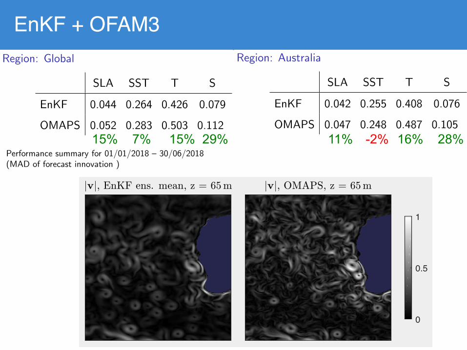
EnKF + OFAM3
Performance summary
Performance summary for 01/01/2018 – 30/06/2018(MAD of forecast innovation )
Region: Global
SLA SST T S
EnKF 0.044 0.264 0.426 0.079
OMAPS 0.052 0.283 0.503 0.112
Region: Australia
SLA SST T S
EnKF 0.042 0.255 0.408 0.076
OMAPS 0.047 0.248 0.487 0.105
6 / 25
Performance summary
Performance summary for 01/01/2018 – 30/06/2018(MAD of forecast innovation )
Region: Global
SLA SST T S
EnKF 0.044 0.264 0.426 0.079
OMAPS 0.052 0.283 0.503 0.112
Region: Australia
SLA SST T S
EnKF 0.042 0.255 0.408 0.076
OMAPS 0.047 0.248 0.487 0.105
6 / 25
Performance summary
Performance summary for 01/01/2018 – 30/06/2018(MAD of forecast innovation )
Region: Global
SLA SST T S
EnKF 0.044 0.264 0.426 0.079
OMAPS 0.052 0.283 0.503 0.112
Region: Australia
SLA SST T S
EnKF 0.042 0.255 0.408 0.076
OMAPS 0.047 0.248 0.487 0.105
6 / 25
15% 15%7% 29% 11% 16%-2% 28%
0
0.5
1

Maritime Continent ModelBrassington, Dietachmayer, Colberg, Zeiger, Sakov, Aijaz, Bende-Mihl, Sun and Roff
Design• Atmosphere, Ocean & Wave
• UM (ACCESS-C), ROMS, WWIII• Ocean data assimilation (EnOI)• Large fixed priority regions O(30 x 30)
• Operate Bureau infrastructure• Secure to third party• Better resolve internal tide climate
• High resolution ~1/50° x 1/50°• Added value• Comparable cost to global model• HPC application
• Pre-configured and optimised• Multi-year hindcasts/reanalyses• Routine operation
• Secure to third party• e.g., MCM 112.4E-142.4E, 19.1S-7.7N
see talk AMOS-2019

MCM configuration - summary
Atmosphere
Unified Model v10.6
80 terrain-following levelsTop of model 38.5 km
Full Euler (non-hydro)Semi-implicit/Semi-LagrangianExplicit convectionOptions:RA1-T (physics - tropics)RA1-M (physics – mid-lat)
Boundary conditionsAPS2 ACCESS-R
Initial conditionsDownscaling ACCESS-R
Ocean
ROMS
30 sigma-levelsSRTM30+ bathymetry
HydrostaticMellor-YamadaAKIMA advection
Forcing (options)ACCESS-R (RT1)ACCESS-MCM (RT2)
Boundary conditionsOceanMAPSTPXO7.2Dai and Trenberth, rivers
Initial conditionsDownscaling OceanMAPS
Wave
WAVEWATCH IIIimplicit
Variable grid (525,836)
29 freq bins (0.035-0.5047)
Directional inc 10d (36)
SRTM30+ bathymetry
Forcing (options)ACCESS-RACCESS-MCM
Boundary conditionsAUSWAVE-R
AUSTRALIAN BUREAU OF METEOROLOGY
ADEPT_Demonstration_Final_Report_Rev2.docx 35
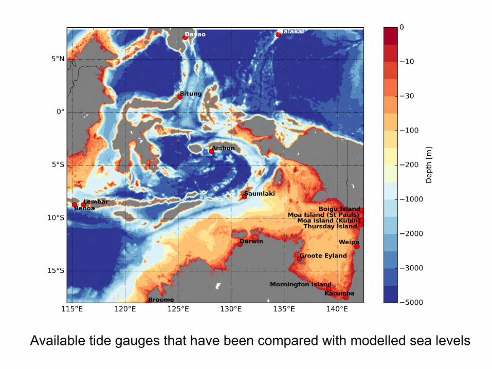
Figure 20: Spatial map of the ADEPT domain. Contours indicate depth of bathymetry. Red dots indicate locations of available tide gauges that have been compared to modelled sea levels.
Available tide gauges that have been compared with modelled sea levels

AUSTRALIAN BUREAU OF METEOROLOGY
ADEPT_Demonstration_Final_Report_Rev2.docx 36
Name Coordinates TimeAvail Source RMSE[m] MAD[m] Rmax(Lag) HAT[m]Davao(Philippines) 125.669,7.07 Jan-Feb2018 UniH. 0.15,0.17 0.13,0.13 0.96(1),0.95(1) 1.08Lembar(Indonesia) 116.069,-8.736 Jan-Feb2018 UniH. 0.10,0.11 0.08,0.08 0.97(0),0.96(0) 0.93Benoa(Indonesia) 115.209,-8.755 Jan-Feb2018 UniH. 0.26,0.26 0.220.22 0.99(1)0.99(1) 1.35Ambon(Indonesia) 128.15,-3.687 Jan-Feb2018 UniH. 0.19,0.20 0.16,0.16 0.94(0),0.94(0) 1.08Saumlaki(Indonesia) 131.26,-7.982 Jan-Feb2018 UniH. 0.23,0.23 0.2,0.2 0.93(1),0.94(1) 1.27Bitung(Indonesia) 125.193,1.44 Jan-Feb2018 UniH. 0.17,0.16 0.140.14 0.96(1),0.96(1) 0.87Malakal(Palau) 134.463,7.33 Jan-Mar2018 UniH. 0.12,0.13 0.09,0.10 0.97(0),0.96(0) 1.05Broome 122.218,-18.00 Jan-Mar2018 BoM NA NA NA NADarwin 130.845,-12.471 Jan-Mar2018 BoM 0.43,0.46 0.34,0.35 0.97(0),0.97(25) 3.65GrooteEyland 136.4158,-13.86 Jan-Mar2018 BoM 0.17,0.19 0.14,0.14 0.9(1),0.86(1) 0.67WeipaTide 141.8622,-12.67 Jan-Mar2018 BoM 0.22,0.24 0.18,0.19 0.95(0),0.93(0) 1.12ThursdayIsland 142.216,-10.583 9Feb-Mar2018 BoM 0.41,0.41 0.34,0.34 0.83(23),0.82(23) 1.61MoaIsland(Kubin) 142.214,-10.236 9Feb-Mar2018 BoM 0.25,0.26 0.20,0.20 0.90(0),0.90(0) 1.55BoiguIsland 142.253,-9.2436 9Feb-Mar2018 BoM 0.27,0.27 0.21,0.21 0.94(0),0.94(0) 1.82MoaIsland(STPauls) 142.334,-10.195 17Feb-Mar2018 BoM 0.31,0.31 0.25,0.25 0.91(0),0.90(0) 1.64KarumbaTide 140.834,-17.488 Jan-Mar2018 BoM 0.36,0.37 0.29,0.30 0.96(1),0.95(1) 1.67MorningtonIsland 139.17,-16.667 Jan-Mar2018 BoM 0.25,0.27 0.21,0.21 0.97(1),0.94(1) 1.09
Mean 0.24, 0.25 0.20, 0.20 0.94, 0.93
Table 8: Available tide gauges. Root Mean Square Error (RMSE), Mean Absolute Difference (MAD), Maximum Correlation (Rmax) and highest astronomical tide (HAT) are shown for RT1 and RT2.
20-25%
10-20%

Internal tides - surface expression and transects
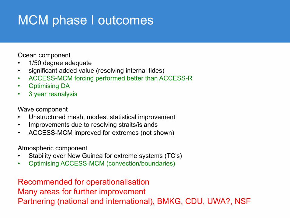
MCM phase I outcomes
Ocean component • 1/50 degree adequate• significant added value (resolving internal tides)• ACCESS-MCM forcing performed better than ACCESS-R• Optimising DA• 3 year reanalysis
Wave component• Unstructured mesh, modest statistical improvement• Improvements due to resolving straits/islands• ACCESS-MCM improved for extremes (not shown)
Atmospheric component• Stability over New Guinea for extreme systems (TC’s)• Optimising ACCESS-MCM (convection/boundaries)
Recommended for operationalisationMany areas for further improvementPartnering (national and international), BMKG, CDU, UWA?, NSF

29
Comparison of regional and MCM wave predictionBetter resolved island groups and straits
Improved representation of fine scale winds
MCM Wave
30
AUSTRALIAN BUREAU OF METEOROLOGY
ADEPT_Demonstration_Final_Report_Rev2.docx 29
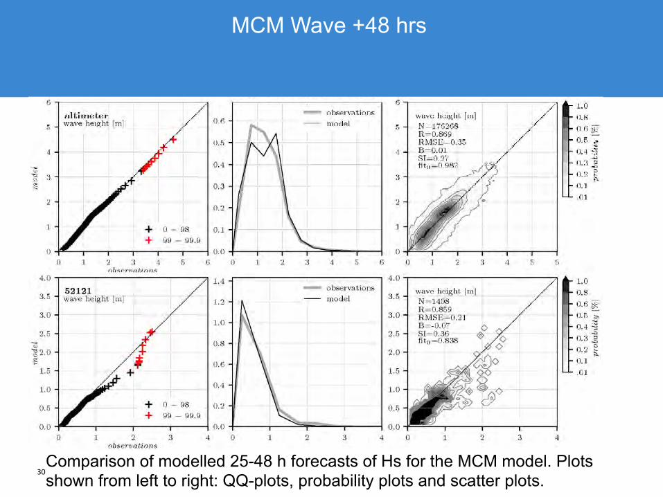
Figure 15 Comparison of modelled (1-24h forecasts) significant wave height (Hs in units of m) relative to observations from altimeters (top panels) and Albatross Bay buoy (52121, bottom panels) for the ADEPT model. Panels show (from left) QQ-plots, probability density plots and scatter density plots. Legend in the far right panels show the goodness of fit by means of number colocations (N)m correlation (R), root-mean-square error (RMSE), bias (B), scatter index (SI) and least-square fit through origin (fit0).
Figure 16 Comparison of modelled 25-48 h forecasts of Hs for the ADEPT model. Plots shows from left to right: QQ-plots, probability plots and scatter density plots. Legend in the far right panel shows the goodness of fit (see caption of Error! Reference source not found.).
MCM Wave +48 hrs
Comparison of modelled 25-48 h forecasts of Hs for the MCM model. Plots shown from left to right: QQ-plots, probability plots and scatter plots.
31
AUSTRALIAN BUREAU OF METEOROLOGY
ADEPT_Demonstration_Final_Report_Rev2.docx 30
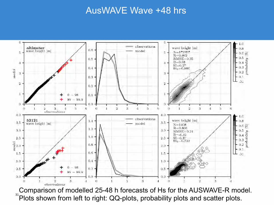
Figure 17 Comparison of modelled 1-24 h forecasts of Hs for the AUSWAVE-R model. Plots shows from left to right: QQ-plots, probability plots and scatter density plots. Legend in the far right panel shows the goodness of fit (see caption of Error! Reference source not found.).
Figure 18 Comparison of modelled 25-48 h forecasts of Hs for the AUSWAVE-R model. Plots shows from left to right: QQ-plots, probability plots and scatter density plots. Legend in the far right panel shows the goodness of fit (see caption of Error! Reference source not found.).
AusWAVE Wave +48 hrs
Comparison of modelled 25-48 h forecasts of Hs for the AUSWAVE-R model. Plots shown from left to right: QQ-plots, probability plots and scatter plots.

Multiscale Data Assimilation in Bluelink Reanalysis (BRAN)
Matt Chamberlain CSIRO, Ocean and Atmosphere, Hobart,
and Bluelink Global Modelling Team.Peter Oke, Gary Brassington, Paul Sandery, Russ Fiedler, Prasanth
Divakaran
Forum for Operational OceanographyOct. 2019.

Multiscale DA Overview • BRAN runs simulate the state of the global ocean at
0.1-degree resolution over the past decades.
• There is significant improvement in the fit of the simulated ocean to observations using 2-stage, multiscale data assimilation process.
• Calculating corrections at coarse resolution is effective at reducing biases in the subsurface.
• Mean absolute errors in subsurface temperature are reduced by up to 33% and 13% for analysis and forecast (3-day) fields respectively.

Introduction
• Output from OFAM spinups and reanalyses publicly available on NCI data catalogue.https://geonetwork.nci.org.au and search OFAM/BRAN.
• OBJECTIVE: Noted that large features (> mesoscale) in thermocline not being corrected for efficiently in current data assimilation system. Want to make better use of subsurface observations (ARGO).
• Bluelink Project, a partnership since 2001 between CSIRO, BoM, and RAN; supporting development of operational ocean forecasting services for Australia.
• OFAM3 platform, near-global 0.1 deg resolution ocean model (Oke et al., GMD, 2013).
• Bluelink Reanalysis (BRAN) experiments, simulate the mesoscale ocean state over the past decades, assimilating SST, sea level, and subsurface T+S profiles; e.g. Oke et al. Ocean Modelling 2018. (~ OceanMAPS from BoM.)
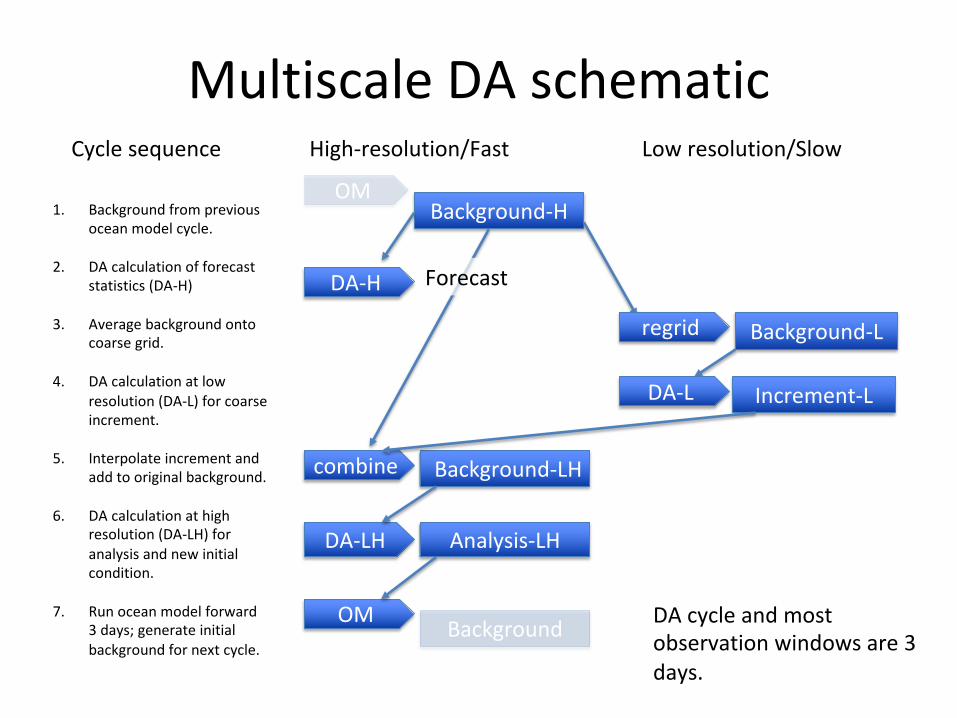
Multiscale DA schematicHigh-resolution/Fast Low resolution/SlowCycle sequence
Background-H1. Background from previous ocean model cycle.
2. DA calculation of forecast statistics (DA-H)
3. Average background onto coarse grid.
4. DA calculation at low resolution (DA-L) for coarse increment.
5. Interpolate increment and add to original background.
6. DA calculation at high resolution (DA-LH) for analysis and new initial condition.
7. Run ocean model forward 3 days; generate initial background for next cycle.
Background-L
Background-LH
Increment-L
Analysis-LH
regrid
DA-LH
DA-H
DA-L
combine
OM
OM
Forecast
Background DA cycle and most observation windows are 3 days.

BRAN Multiscale DA - ensemble correlation
1-de
gO
FAM
BRAN data assimilation uses Ensemble Optimal Interpolation (EnOI). An ensemble of anomalies from a previous model run is used to apply corrections to the model state, in space and across different ocean variables.
Shown here are examples of covariance from each ensemble set
• OFAM ensemble “3-day minus 3-month average”; captures eddies and mesoscale variability.
• ACCESS 1-deg ensemble of monthly climatological anomalies from 40-years of ocean-ice model with historical forcing (JRA-55); captures broad 100+ km scale variability.

Global Mean Absolute Deviations -forecast and analysis
• Multiscale statistics shown for Jan-Jun 2018.
• Little change in surface fields which are well observed.
• Substantial improvement in subsurface.

Global Mean Absolute Deviations - forecast and analysis
BRAN2015 Multiscale
Analysis Forecast Analysis Forecast
SST (C)0.139 0.304 0.141 +1.0% 0.315 +3.6%
Sea height (cm)2.85 5.22 2.74 -4.0% 5.13 -1.9%
Subsurface temperature (C) 0.308 0.519 0.204 -33.8% 0.449 -13.5%
Subsurface salinity (psu) 0.0586 0.1003 0.039 -33.4% 0.0817 -18.5%
• Statistics averaged over Jan-Jun 2018.
• Little change in surface fields, which are well observed. Slight degradation of SST, improvement in sea level corresponding to a better ocean interior.
• Substantial improvement in statistics from subsurface.

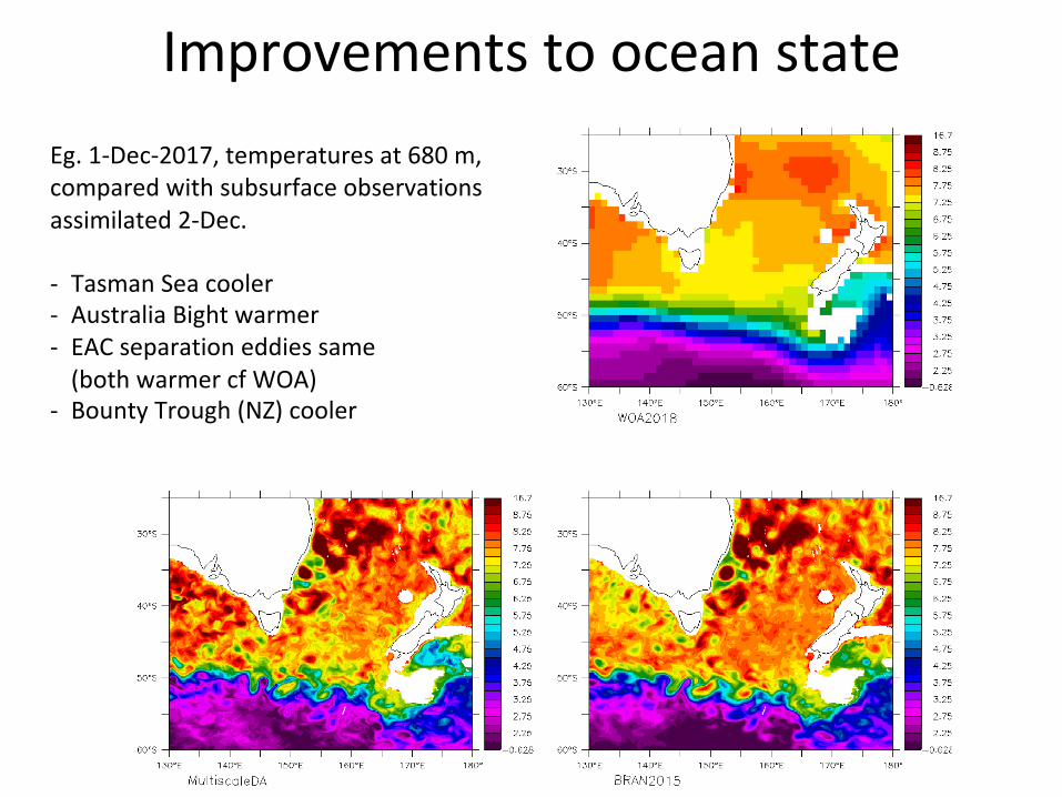
Improvements to ocean stateEg. 1-Dec-2017, temperatures at 680 m,compared with subsurface observations assimilated 2-Dec.
- Tasman Sea cooler- Australia Bight warmer- EAC separation eddies same
(both warmer cf WOA)- Bounty Trough (NZ) cooler
Improvements to ocean stateEg. 1-Dec-2017, temperatures at 680 m,compared with subsurface observations assimilated 2-Dec.
- Tasman Sea cooler- Australia Bight warmer- EAC separation eddies same
(both warmer cf WOA)- Bounty Trough (NZ) cooler

Improvements to ocean state- Tasman Sea cooler- Australia Bight warmer- EAC separation eddies same
(both warmer cf WOA)- Bounty Trough (NZ) cooler
Eg. 1-Dec-2017, temperatures at 680 m

Discussion• Improvements found in ocean state at depth; surface fields (SST,
SLA) are already well observed/constrained.
• Ideally, DA system would only have to correct for dynamics. In reality, it also corrects for model biases.
• Broader footprints of correlation in the coarse ensemble make the multiscale system more efficient at correcting for these biases.
• DA system is robust and able to use ensembles from different model platforms. It is advantageous to run a coarse model for longer control experiments and ‘cleaner’ climatological anomalies.

Summary• There is significant improvement in BRAN simulations using 2-
stage/multiscale data assimilation process.
• Calculating corrections at coarse resolution is effective at reducing biases in the subsurface where observations are sparse.
• Mean absolute errors in subsurface temperature are reduced by up to 33% and 13% for analysis and forecast (3-day) fields respectively.Improvements are comparable to 100-member EnKF systems for a fraction of the computational cost.
• Apply to future BRAN/OceanMAPS runs.

• Done!

sep19c - global biases

Global Mean Absolute Biases -forecast and analysisBRAN2015 Multi scaleAnalysis Forecast Analysis Forecast
SST (C) -0.007 -0.03 0.141 0.315
Sea height (cm)0.03 -0.05 2.74 5.13
Subsurface temperature (C) -0.043 -0.107 0.204 0.449
Subsurface salinity (psu)
-0.0074 -0.0149 0.039 0.0817

Standard BRAN processHigh-resolution/FastCycle sequence
Background-H1. Background from previous ocean model cycle.
2. DA calculation of forecast and analysis (DA-H) and obtain new initial condition.
7. Run ocean model, generate initial background for next cycle.
Analysis-LHDA-H
OM
OM
Background

DA Cycles and Observation Windows Schematic
days
cycles 0-2 -1 +1 +2
3-daycentered
9-day centered
9-day offset
Offset such that no observations overlap with the forecast statistics (with 3-day window) in next cycle.
10% of subsurface observations in future 3 days withheld for forecast calculation
3-day window used for forecast in next cycle

BRAN Multiscale DA - Ensembles• BRAN ensemble “3-day minus 3-
month average”; captures eddies and mesoscale variability.
• ACCESS 1-deg ensemble of 480 monthly anomalies (wrt. climatology of detrended time series) from 40-years of ocean-ice model with historical forcing (JRA-55); captures broad 1000-km scale variability.


