42
BMME 560 & BME 590I Medical Imaging: X-ray, CT, and Nuclear Methods CT Imaging Part 1
| Date post: | 17-Dec-2015 |
| Category: |
Documents |
| Upload: | kelly-hill |
| View: | 222 times |
| Download: | 2 times |

BMME 560 & BME 590IMedical Imaging: X-ray, CT, and
Nuclear Methods
CT Imaging Part 1

Today
• CT Systems– Seven generations– Instrumentation
• CT Image interpretation– CT number
• CT Degradations– Beam hardening– Metal artifacts– Other issues
CT Systems
• CT system designs are classified into “generations”
• These are more or less in chronological order, but some earlier generations have lasted longer than later ones.
• These are explained well in your book.

CT Generations
1. Scanning pencil beam
2. Scanning fan beam
3. Full fan-beam with rotating detector*
4. Full fan-beam with stationary detector ring*
5. Electron-beam CT (EBCT)
6. Spiral CT*
7. Multislice CT*
* Most common today

Spiral and Multislice CT
The patient moves through the scanner, so that a complete rotation is NOT taken for any given plane. This requires interpolation for the helical data.
The key parameter is the pitch, the axial distance traversed in one complete rotation of the gantry.
Reference 1

Electron-beam CT (EBCT)
Electron source
Magnetic steering
Target ring
Detector ring
No mechanical motion required to obtain tomographic data

CT Instrumentation
• Sources differ from radiography sources– Fan-beam sources have slit collimators to keep
beam in plane• Slit may be adjustable
• This needs to be opened up in multislice CT
– More filtration than in projection radiography• Use a “harder” (higher average energy) beam to reduce
beam hardening artifacts

CT Instrumentation
• Tube-current modulation
Use higher tube current in this position to get the same number of photons on the detector
Use lower tube current here
CT Instrumentation
• Tube voltage selection– Higher tube voltage = higher effective energy
• Less contrast between soft tissues
• Lower dose
– 80 kVp and up to 140 kVp are common– It depends on the reason for the scan and the tissue
properties of the region being imaged.

CT Instrumentation
• Detectors– Solid-state scintillator + photodiode array
– NOT flat-panel, but strip detectors because they have faster readout
– Multislice systems simply stack strips to form slices
• Note that in 3G systems, the slice thickness may be controlled by beam collimation, but in 7G systems it is determined by the detector spacing.

CT Instrumentation
• Slip-ring– To perform spiral/helical CT, we must achieve
continuous rotation of the source and detector– BUT we must also deliver continuous power to the
rotating tube and continuously read data from the rotating detector
– Power is delivered through continuous electrical contact between a stationary ring and a “brush” on the rotating gantry (wearing problem?)
– Data is communicated through optical links

CT Image Reconstruction
• Remember that CT is a transmission imaging modality
• To obtain Radon-type (line integral) data, we have to perform a log-transform
0
0
exp ( )
( ) log
j j
jj
j
I I s ds
Ig s ds
I
Measured data
Blank scan data

CT Image Interpretation
• What does the intensity in the raw reconstructed CT image mean? What are its units?
• Problem: Each X-ray tube has its own spectral characteristics, and the characteristics change over the service life of the tube.– Constant calibration is necessary

Contrast
• Properties of materials

CT Image Interpretation
• Measured values are normalized via the CT number, which is expressed in Hounsfield units (HU)
• But we must measure water under the same conditions (tube voltage, current, time of service, etc) as when the CT is taken
1000 pixel water
water
h

CT Numbers of Common Materials
material Min Max
Bone 400 1000
Soft tissue 40 80
Water 0 0
Fat -100 -60
Lung -600 -400
Air -1000 -1000
Most CT scanners range up to 2000, but some can go up to 4000 to accommodate metal implants. What determines the peak CT number resolvable in a scanner? Reference 1

CT Numbers
• Example problem– If the CT number of bone is 1000,
• What is the relationship between the linear attenuation coefficients of bone and water for this device?
• What is the effective energy of this device for imaging bone?

CT NumbersEnergy(MeV) Water mu (cm^-1) Bone mu (cm^-1) Bone - 2*water
1.00E-02 5.33E+00 54.7392 4.41E+011.50E-02 1.67E+00 17.34144 1.40E+012.00E-02 8.10E-01 7.68192 6.06E+003.00E-02 3.76E-01 2.55552 1.80E+004.00E-02 2.68E-01 1.27776 7.41E-015.00E-02 2.27E-01 0.814464 3.61E-016.00E-02 2.06E-01 0.604416 1.93E-018.00E-02 1.84E-01 0.427968 6.06E-021.00E-01 1.71E-01 0.35616 1.48E-021.50E-01 1.51E-01 0.28416 -1.68E-022.00E-01 1.37E-01 0.251328 -2.27E-023.00E-01 1.19E-01 0.213696 -2.35E-024.00E-01 1.06E-01 0.1902336 -2.20E-025.00E-01 9.69E-02 0.1732224 -2.05E-026.00E-01 8.96E-02 0.1599744 -1.91E-028.00E-01 7.87E-02 0.1403136 -1.70E-021.00E+00 7.07E-02 0.1260672 -1.54E-021.25E+00 6.32E-02 0.1127232 -1.37E-021.50E+00 5.75E-02 0.1026432 -1.24E-022.00E+00 4.94E-02 0.0884544 -1.04E-023.00E+00 3.97E-02 0.071904 -7.48E-034.00E+00 3.40E-02 0.0625344 -5.53E-035.00E+00 3.03E-02 0.0565632 -4.06E-036.00E+00 2.77E-02 0.0524928 -2.91E-038.00E+00 2.43E-02 0.0473664 -1.21E-031.00E+01 2.22E-02 0.0444288 4.88E-051.50E+01 1.94E-02 0.0409344 2.11E-032.00E+01 1.81E-02 0.0397056 3.45E-03

CT Numbers
• Calibration– Frequent calibration of
the system is necessary
– Image a phantom with known material properties, including air and water
– In radiation dosimetry applications, may need to develop a conversion curve to electron density
www.scanditronix-wellhofer.com

CT Limitations
• Deviations from Radon projections– Beam hardening– Partial volume– Photon starvation– Metal artifacts– Motion artifacts– Nonuniformity– Helical scanning– Cone-beam

CT Artifacts
• Beam hardening occurs when low energies are preferentially absorbed by the subject
• The spectrum changes as the beam travels through the subject.
Reference 2

CT Artifacts
• Beam hardening
The beam spectrum reaching the object differs depending on the angle of projection
Also, the response of the detector will vary with energy spectrum

CT Artifacts
• Beam hardening – “cupping” artifact
1
2
Projection line 2 experiences more beam hardening than projection line 1, so line 2 deviates more from the ideal Radon projection. How?

CT Artifacts
• Beam hardening – cupping artifact
Reference 2
In a cylinder, it is possible to calibrate and correct for this. Patients, only partly so.
CT Artifacts
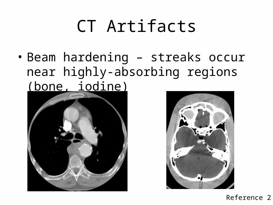
• Beam hardening – streaks occur near highly-absorbing regions (bone, iodine)
Reference 2

CT Artifacts
• Beam hardening – partial correction
Reference 2Iterative correction algorithm determines bony locations and estimates beam hardening effects.

CT Artifacts
• Beam-hardening reduction– Filtration
• Pre-hardening
• Bowtie filter
– Phantom calibration with different shapes– Iterative post-correction methods– Iterative reconstruction
Hardens the beam more at edges to reduce cupping

CT Artifacts
• Partial volume effect– Consider a fan-beam with a certain slice thickness – If an object is only partially in the slice, its
apparent attenuation will be reduced.

CT Artifacts
• Photon starvation – streak artifacts caused by too few photons at some angles
Reference 2

CT Artifacts
• Addressing photon starvation– Get more photons
• Tube current modulation
– “Adaptive filtration”• Pre-reconstruction method for identifying low-count
regions and (linear, not radiation) filtering in axial direction selectively

CT Artifacts
• Adaptive filtration – partial correction
Reference 2

CT Artifacts
• Metal artifacts – both photon starvation and beam hardening
Reference 2

CT Artifacts
• Even though a slice can be completed in 1-2 seconds (or less on newer systems), patient motion is significant– Voluntary motion (wiggly patients)– Involuntary motion (heartbeat, respiration)
• If the motion is rigid-body motion, and we know the transformation, we can correct it.

CT Artifacts
• Motion artifact
Reference 2

CT Artifacts
• Rigid-body voluntary motion
Translation
Rotation

CT Artifacts
• Most software-correction methods for voluntary motion are based on rigid-body transforms
• Estimate the motion by using the beginning and end projections
• Apply the rigid-body transform to the backprojection geometry in reconstruction
• Note that people are not necessarily rigid

CT Artifacts
• Motion correction
Reference 2

CT Artifacts
• Detector nonuniformity – ring artifacts
Reference 2

CT Artifacts
• Helical scanning – artifacts occur around regions that vary quickly in axial direction – depending on helical pitch and slice thickness – due to angle-varying partial volume effects
Reference 2

CT Artifacts
• Cone-beam artifacts: Multislice scanners suffer more from cone-beam oblique angle artifacts
Reference 2

CT Artifacts
• Key points– Many factors can contribute to inconsistencies in
the data.• Be able to explain the physical reasons why the artifacts
occur and why they are inconsistent.
– Frequent calibration can help.– Experienced operators are essential.

References
1. S. Jackson, R. M. Thomas, Cross-sectional Imaging Made Easy, Churchill Livingstone: London, 2004.
2. J. F. Barrett, N. Keat, “Artifacts in CT: Recognition and Avoidance,” Radiographics, vol. 24, pp. 1679-1691, 2004.


