1. Introduction

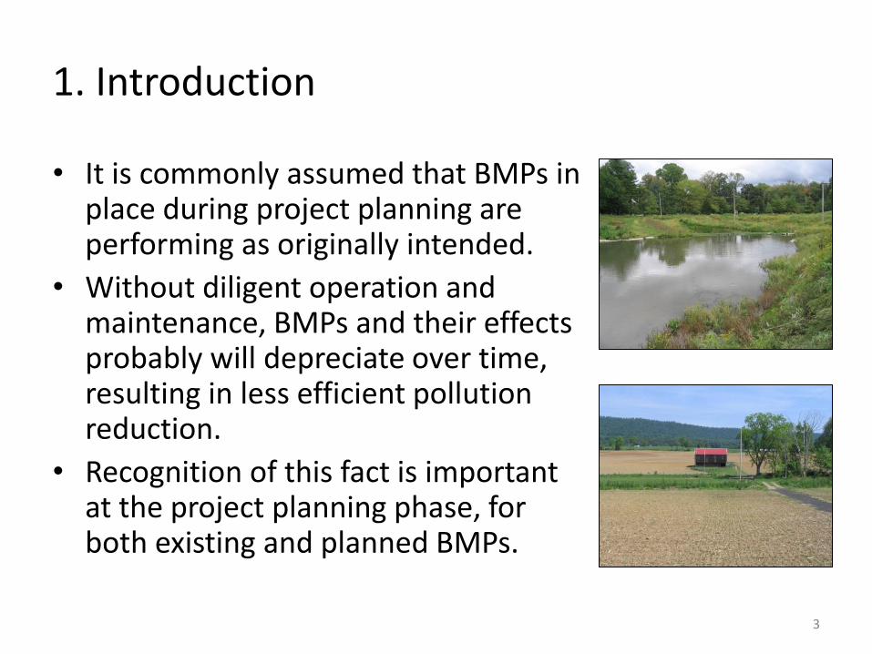
• It is commonly assumed that BMPs in place during project planning are performing as originally intended.

• Without diligent operation and maintenance, BMPs and their effects probably will depreciate over time, resulting in less efficient pollution reduction.

• Recognition of this fact is important at the project planning phase, for both existing and planned BMPs.

3

1. Introduction

• Watershed planning must fully assess contributing causes and sources of pollution, then prioritize strategies to address the problems

• EPA nine key elements for 319 implementation projects: – Identify causes/sources of

impairment; – Describe BMPs needed to achieve

required load reductions; – Define critical areas where BMPs to

be implemented; and – Estimate load reductions expected

from BMPs

4 (USEPA 2008, 2013)

1. Introduction

• Achieving these requirements depends on accurate information on the performance levels of both BMPs already in place and BMPs to be implemented as part of the watershed project.

• BMPs credited during the planning phase of a watershed project will be expected to continue to provide planned water quality benefits as part of the overall plan to protect or restore a water body.

5

1. Introduction

• Verification that BMPs are still performing their functions at anticipated levels and if or how they have depreciated is essential: – To inform decisions about needs for

additional BMPs; – To understand needs for repair of existing

BMPs and maintenance of new BMPs; and

– To use adaptive management to keep a project on track to achieve its overall goals.

6

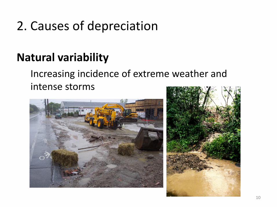
2. Causes of depreciation

Natural variability

Climate and soil variations

7

2. Causes of depreciation

Natural variability

Seasonal dormancy

8

2. Causes of depreciation

Natural variability

Year-to-year variation in precipitation

9

2. Causes of depreciation

Natural variability

Increasing incidence of extreme weather and intense storms

10

2. Causes of depreciation

11

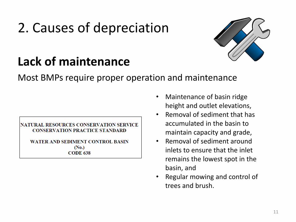
Lack of maintenance Most BMPs require proper operation and maintenance

• Maintenance of basin ridge

height and outlet elevations, • Removal of sediment that has

accumulated in the basin to maintain capacity and grade,

• Removal of sediment around inlets to ensure that the inlet remains the lowest spot in the basin, and

• Regular mowing and control of trees and brush.

2. Causes of depreciation

12

Lack of maintenance Most BMPs require proper operation and maintenance

Annual operation and maintenance inspection of wet ponds. • Excessive sediment, debris, or trash

accumulated at inlet, • Clogging of outlet structures, • Cracking, erosion, or animal burrows in

berms, and • >1 foot of sediment accumulated in

permanent pool.

2. Causes of depreciation

13

Lack of maintenance Detention pond sediment forebay

2. Causes of depreciation

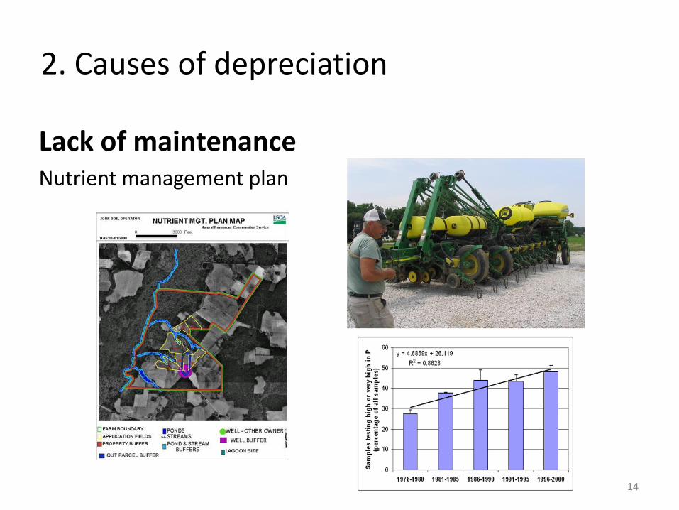
14

Lack of maintenance Nutrient management plan

2. Causes of depreciation

15

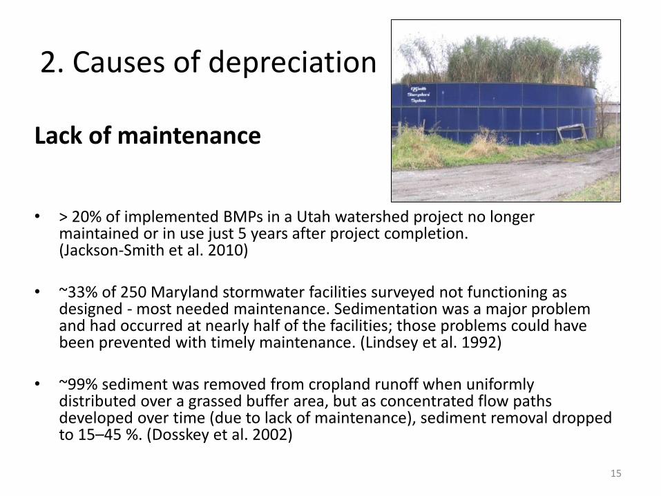
Lack of maintenance

• > 20% of implemented BMPs in a Utah watershed project no longer maintained or in use just 5 years after project completion. (Jackson-Smith et al. 2010)

• ~33% of 250 Maryland stormwater facilities surveyed not functioning as designed - most needed maintenance. Sedimentation was a major problem and had occurred at nearly half of the facilities; those problems could have been prevented with timely maintenance. (Lindsey et al. 1992)

• ~99% sediment was removed from cropland runoff when uniformly distributed over a grassed buffer area, but as concentrated flow paths developed over time (due to lack of maintenance), sediment removal dropped to 15–45 %. (Dosskey et al. 2002)

2. Causes of depreciation

16

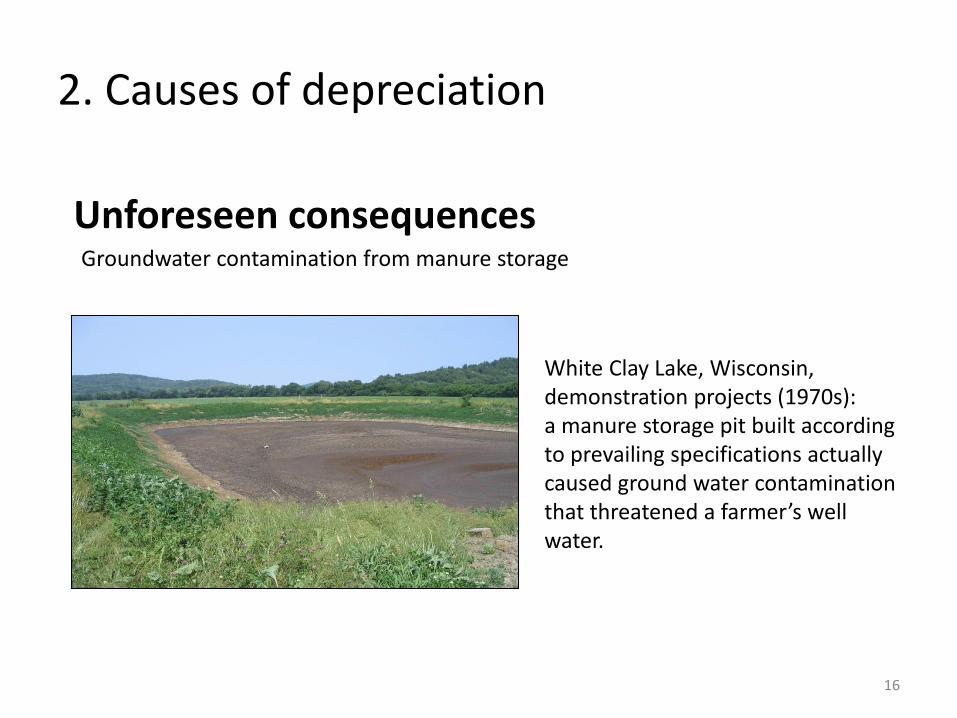
Unforeseen consequences

Groundwater contamination from manure storage

White Clay Lake, Wisconsin, demonstration projects (1970s): a manure storage pit built according to prevailing specifications actually caused ground water contamination that threatened a farmer’s well water.

2. Causes of depreciation

17

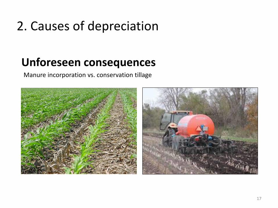
Unforeseen consequences

Manure incorporation vs. conservation tillage

2. Causes of depreciation

18

Unforeseen consequences

Control of peak vs. bankfull urban stormflows

Although large peak stormflows may be controlled effectively by detention storage, the duration of erosive and bankfull conditions are actually extended over longer time period. These flows accumulate downstream and increase peak flows along receiving waters. This diminishes the collective effectiveness of detention basins. (Urbonas and Wulliman 2007)

3. Assessment of depreciation

The first—and possibly most important—step in adjusting for depreciation of implemented BMPs is to determine its extent and magnitude through BMP verification.

19

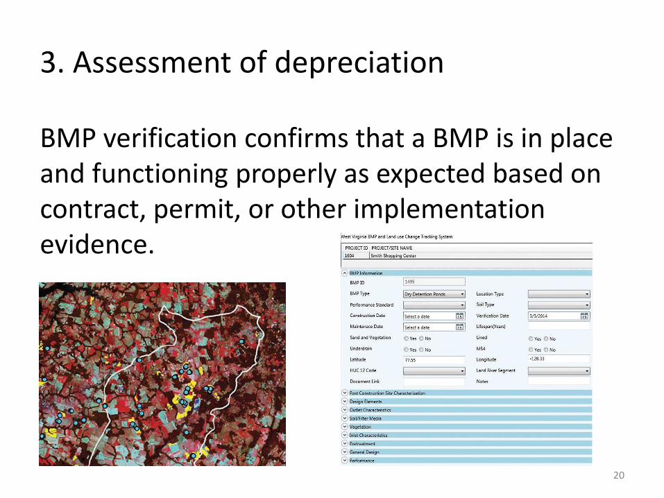
3. Assessment of depreciation

BMP verification confirms that a BMP is in place and functioning properly as expected based on contract, permit, or other implementation evidence.

20

3. Assessment of depreciation

• A BMP verification process that documents the presence and function of BMPs over time should be included in all NPS watershed projects.

– At the project planning phase, verification is important both to ensure accurate assessment of existing BMP performance levels and to determine additional BMP and maintenance needs.

– Verification over time is necessary to determine if BMPs are maintained and operated during the period of interest.

21

3. Assessment of depreciation

22

http://www.bae.ncsu.edu/programs/extension/wqg/319monitoring/tech_notes.htm

3.a. Assessment for Project Planning

• Purpose: To develop accurate information on the performance levels of BMPs already in place to ensure that: – BMP crediting is accurate – Plans for additional BMPs complement existing BMPs to

achieve water quality/quantity goals

• Develop a plan in collaboration with programs and individuals or groups implementing and managing the BMPs – Set a verification timeline that works with the BMP

implementation timeline – Work within available resource limitations: set priorities

23

3.a. Assessment for Project Planning

• Factors to consider in setting priorities:

– Absolute/relative load reductions and locations within pollutant delivery system

• E.g., Chesapeake Bay Program – 100% initial verification of all BMPs

– 10% follow-up verification of multi-year BMPs that contribute 5% or more of nutrient or sediment load reduction

– 20% follow-up verification for permit-based BMPs

– 5% follow-up verification of BMPs contributing <5%

– Critical source areas and subwatersheds

24

3.a. Assessment for Project Planning

• Factors to consider in setting priorities (cont.): – Risky practices: focus on practices with a

documented history of failure over time, more demanding operation and maintenance requirements, or a tendency to be abandoned

– Practice age (more later)

– Cost: focus on practices for which replacement costs (absolute or per unit load reduction) may be greatest if found later to not be performing as expected

25

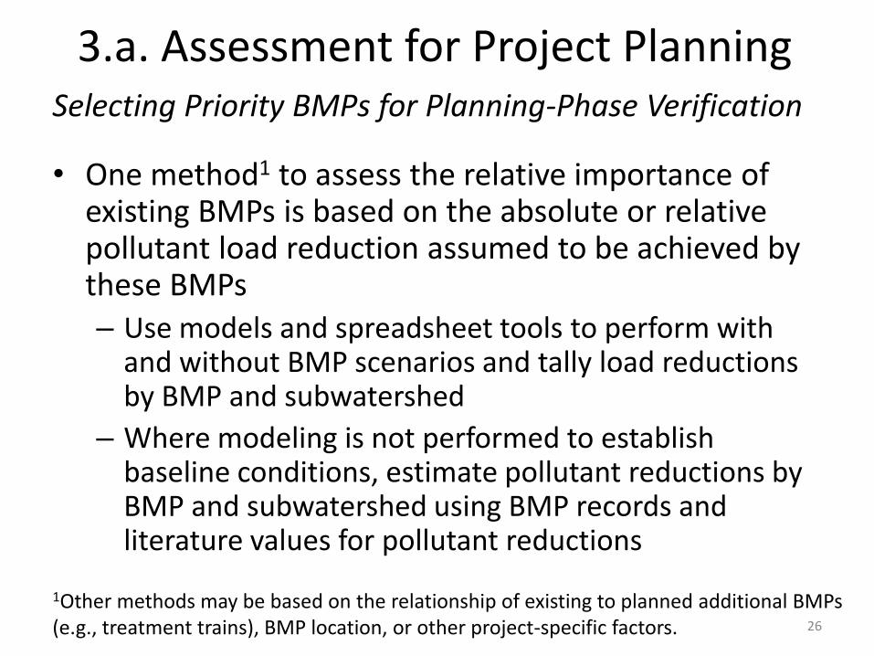
3.a. Assessment for Project Planning

• One method1 to assess the relative importance of existing BMPs is based on the absolute or relative pollutant load reduction assumed to be achieved by these BMPs – Use models and spreadsheet tools to perform with

and without BMP scenarios and tally load reductions by BMP and subwatershed

– Where modeling is not performed to establish baseline conditions, estimate pollutant reductions by BMP and subwatershed using BMP records and literature values for pollutant reductions

26

1Other methods may be based on the relationship of existing to planned additional BMPs (e.g., treatment trains), BMP location, or other project-specific factors.

Selecting Priority BMPs for Planning-Phase Verification

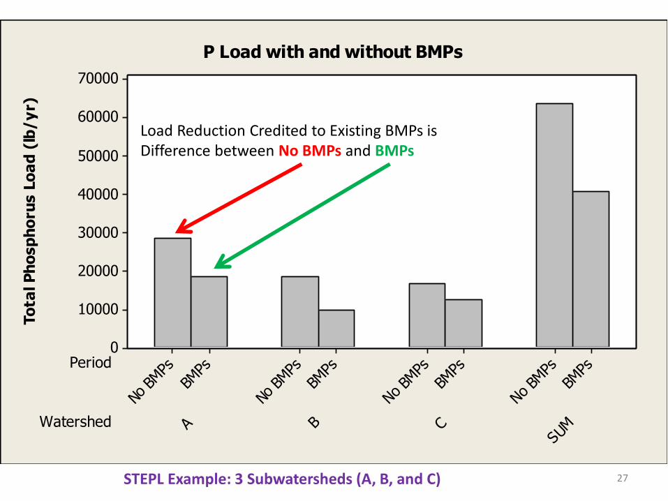
Watershed

Period

SUMCBA

BMPs

No BMPs

BMPs

No BMPs

BMPs

No BMPs

BMPs

No BMPs

70000

60000

50000

40000

30000

20000

10000

0

To

tal P

ho

sp

ho

rus L

oa

d (

lb/

yr)

P Load with and without BMPs

Load Reduction Credited to Existing BMPs is Difference between No BMPs and BMPs

STEPL Example: 3 Subwatersheds (A, B, and C) 27

11

31

4

1

8 9

0

8

21

2 1

2

7

0 0

5

10

15

20

25

30

35

Tota

l P (

1,0

00

lb/y

r)

Total P Load by Source Category

No BMPs

BMPs

STEPL Example: Load reductions broken down by source category 28

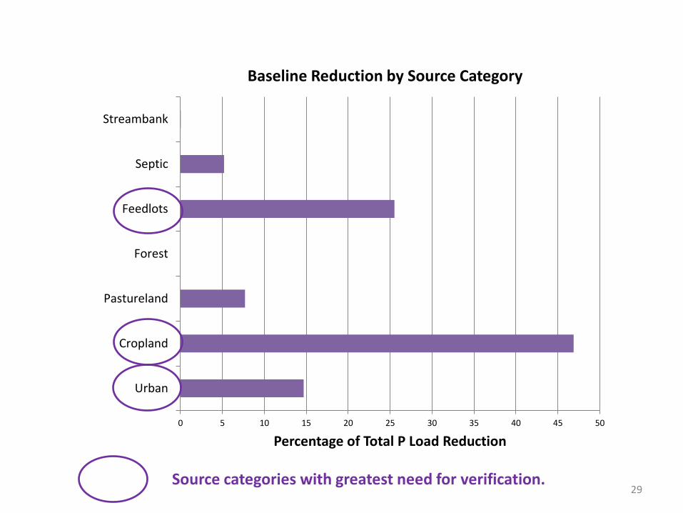
0 5 10 15 20 25 30 35 40 45 50

Urban

Cropland

Pastureland

Forest

Feedlots

Septic

Streambank

Percentage of Total P Load Reduction

Baseline Reduction by Source Category

Source categories with greatest need for verification. 29

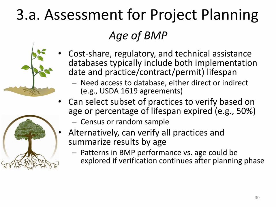
Age of BMP

• Cost-share, regulatory, and technical assistance databases typically include both implementation date and practice/contract/permit) lifespan – Need access to database, either direct or indirect

(e.g., USDA 1619 agreements)

• Can select subset of practices to verify based on age or percentage of lifespan expired (e.g., 50%) – Census or random sample

• Alternatively, can verify all practices and summarize results by age – Patterns in BMP performance vs. age could be

explored if verification continues after planning phase

30

3.a. Assessment for Project Planning

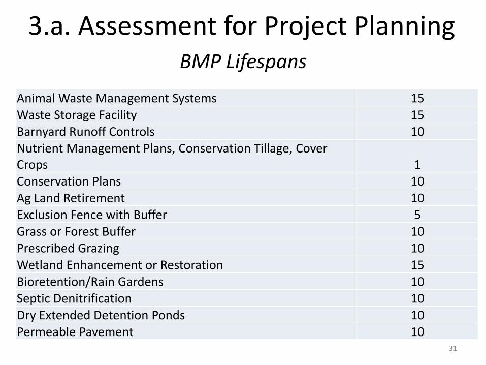
BMP Lifespans

31

Animal Waste Management Systems 15 Waste Storage Facility 15 Barnyard Runoff Controls 10 Nutrient Management Plans, Conservation Tillage, Cover Crops 1 Conservation Plans 10 Ag Land Retirement 10 Exclusion Fence with Buffer 5 Grass or Forest Buffer 10 Prescribed Grazing 10 Wetland Enhancement or Restoration 15 Bioretention/Rain Gardens 10 Septic Denitrification 10 Dry Extended Detention Ponds 10 Permeable Pavement 10

3.a. Assessment for Project Planning

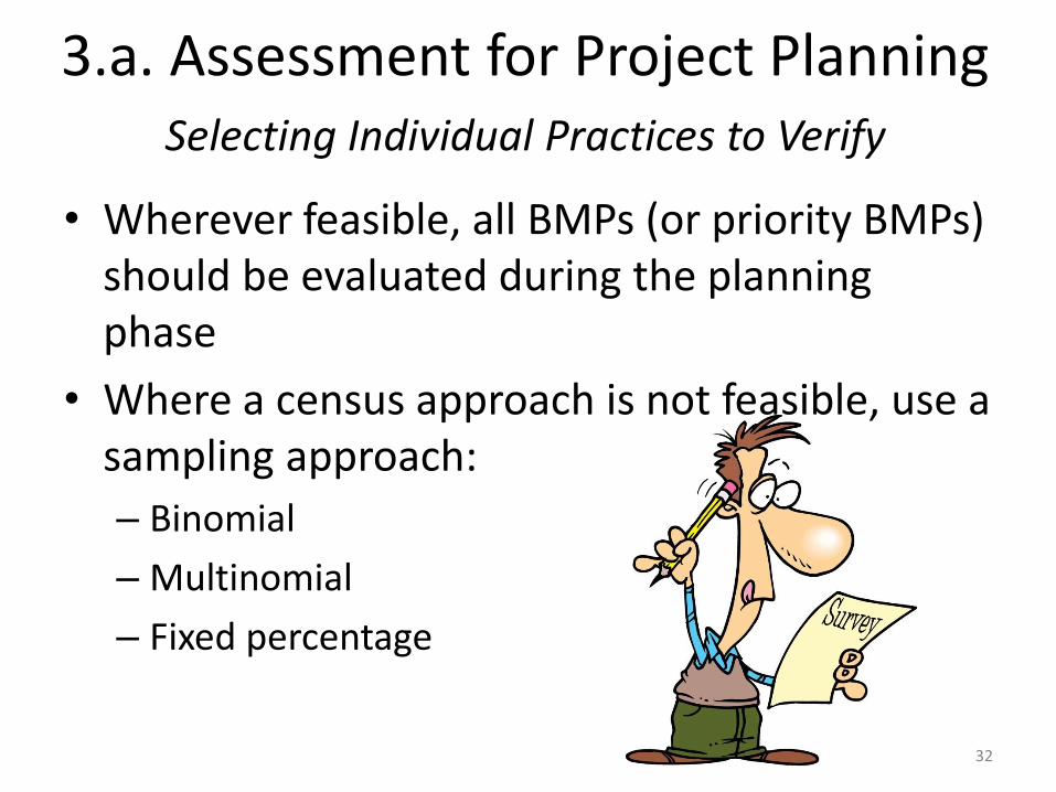
Selecting Individual Practices to Verify

• Wherever feasible, all BMPs (or priority BMPs) should be evaluated during the planning phase

• Where a census approach is not feasible, use a sampling approach:

– Binomial

– Multinomial

– Fixed percentage

32

3.a. Assessment for Project Planning

Binomial Sampling Approach

• Binomial Distribution (two options) – Are the BMPs still there?

• Yes/No

– Are the BMPs still functioning properly? • Yes/No

• Sample Size—just like political polls

33

± 2%

± 4%

±5% ±10%

± 3%

n=2,401

n=1,067

n=600

n=384 n=96

Source: http://en.wikipedia.org/wiki/Margin_of_error#Calculations_assuming_random_sampling

Margin of Error Sample Size

3.a. Assessment for Project Planning

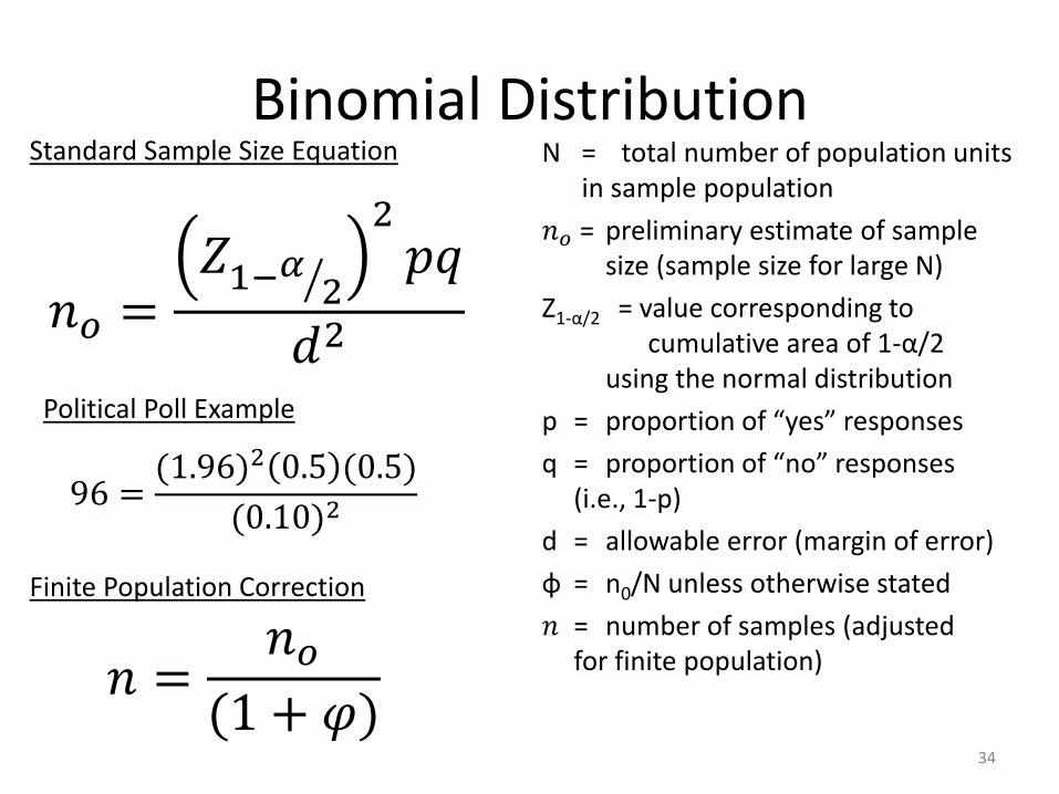
Binomial Distribution N = total number of population units in sample population

𝑛𝑜 = preliminary estimate of sample size (sample size for large N)

Z1-α/2 = value corresponding to cumulative area of 1-α/2 using the normal distribution

p = proportion of “yes” responses

q = proportion of “no” responses (i.e., 1-p)

d = allowable error (margin of error)

φ = n0/N unless otherwise stated

𝑛 = number of samples (adjusted for finite population)

34

𝑛𝑜 =𝑍1−𝛼 2

2𝑝𝑞

𝑑2

𝑛 =𝑛𝑜

(1 + 𝜑)

96 =(1.96)2 0.5 (0.5)

(0.10)2

Standard Sample Size Equation

Finite Population Correction

Political Poll Example

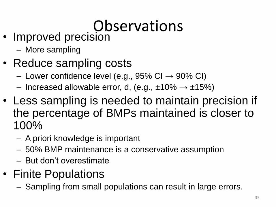
Observations • Improved precision

– More sampling

• Reduce sampling costs – Lower confidence level (e.g., 95% CI → 90% CI)

– Increased allowable error, d, (e.g., ±10% → ±15%)

• Less sampling is needed to maintain precision if the percentage of BMPs maintained is closer to 100% – A priori knowledge is important

– 50% BMP maintenance is a conservative assumption

– But don’t overestimate

• Finite Populations – Sampling from small populations can result in large errors.

35

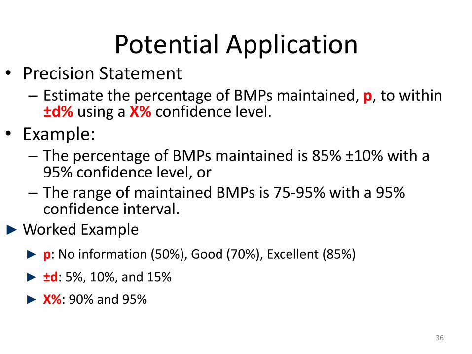
Potential Application • Precision Statement

– Estimate the percentage of BMPs maintained, p, to within ±d% using a X% confidence level.

• Example: – The percentage of BMPs maintained is 85% ±10% with a

95% confidence level, or – The range of maintained BMPs is 75-95% with a 95%

confidence interval. ► Worked Example

► p: No information (50%), Good (70%), Excellent (85%)

► ±d: 5%, 10%, and 15%

► X%: 90% and 95%

36

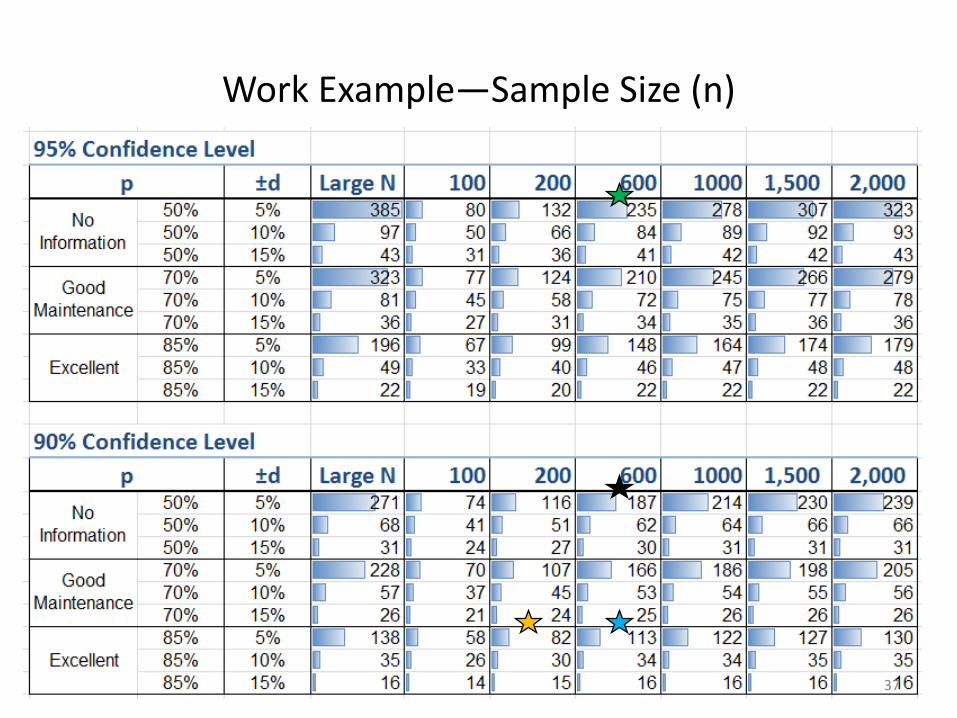
Work Example—Sample Size (n)

37

Multinomial Sampling Approach

• In a multinomial distribution there are more than two mutually exclusive options

• For example, a multinomial distribution may include the following three options: – BMP is there and performing as expected

– BMP is there but not performing as expected

– BMP is not there

• Basis for CTIC Cropland Transect Survey Method sample size determination (Hill 1996, Tortora 1978)

38

3.a. Assessment for Project Planning

Multinomial Distribution

39

Sample Size Equation

𝑛 = sample size

= Chi-square value for one d.f. and the value (1-(a/k))

substituted for (1-α)

a = 1-p

p = confidence level for each category (equivalent to 1- α for binomial)

k = number of categories

p = proportion of “yes” responses

q = a priori estimate of the proportion for each category (as a decimal). Use the q value for the category closest to 0.50 to ensure that sample size is sufficient for all categories. Use 0.50 when unknown. (q is the same as p for the binomial calculation).

d = allowable error in the proportions (e.g., +/- 10%), expressed as a decimal (same as d for binomial calculation)

Observations • Sample size increases as number of categories

increases (not linear)

• Sample size decreases as error margin increases

• Less sampling is needed to maintain precision if the

percentage of BMPs maintained is closer to 100%

– A priori knowledge is important

– 50% BMP maintenance is a conservative assumption

– But don’t overestimate

40

0

200

400

600

800

1000

0 10 20 30

Potential Application • Precision statement for each factor

• Can address multiple questions or variables (i.e., factors) when assessing existing BMPs

– Is the BMP there?

– Does the BMP still meet design standards and specifications?

– Is the BMP designed for the water quality/quantity objectives of the project?

41

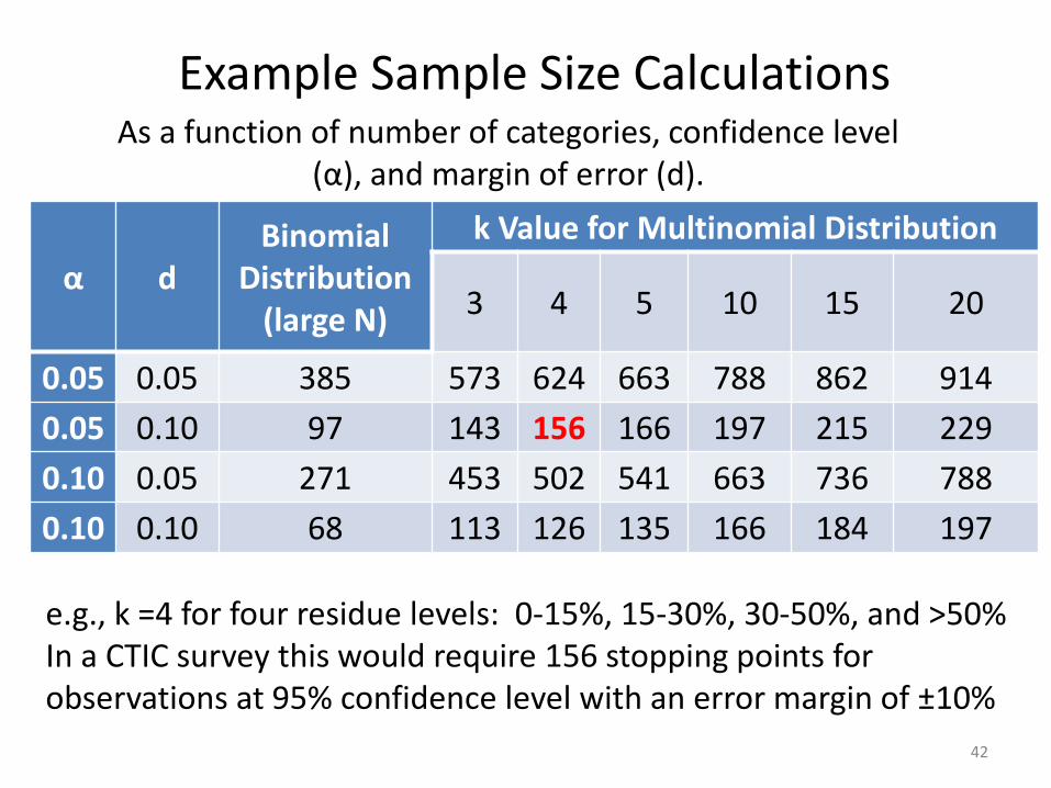
Example Sample Size Calculations

42

α d

Binomial Distribution

(large N)

k Value for Multinomial Distribution

3 4 5 10 15 20

0.05 0.05 385 573 624 663 788 862 914

0.05 0.10 97 143 156 166 197 215 229

0.10 0.05 271 453 502 541 663 736 788

0.10 0.10 68 113 126 135 166 184 197

As a function of number of categories, confidence level (α), and margin of error (d).

e.g., k =4 for four residue levels: 0-15%, 15-30%, 30-50%, and >50% In a CTIC survey this would require 156 stopping points for observations at 95% confidence level with an error margin of ±10%

Fixed Percentage Sampling

• USDA-NRCS verifies 100 percent of practices at installation and an annual minimum of 5 percent of total practices installed or reported in each State

– NRCS has a rigorous protocol for verifying practices

– Statistical significance and error margins of the 5 percent sampling are not advertised

43

3.a. Assessment for Project Planning

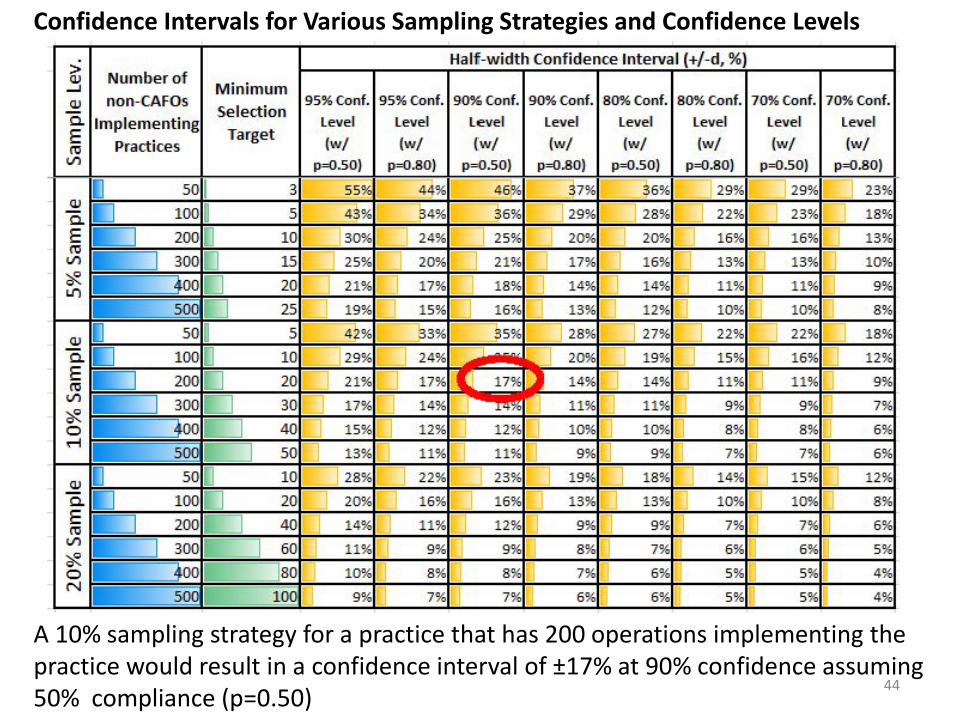
Confidence Intervals for Various Sampling Strategies and Confidence Levels

A 10% sampling strategy for a practice that has 200 operations implementing the practice would result in a confidence interval of ±17% at 90% confidence assuming 50% compliance (p=0.50)

44

> Halfr-width Confidence Interval (+/-d, %) Q) Number of

Minimum -' Q) non-CAFOs

Selection 95%Conf. 95%Conf. 90%Conf. 90%Conf. 80%Conf. 80%Conf. 70%Conf. 70%Conf.

c. Implementing l evel l evel l e vel l evel l evel l evel l evel l evel E Practices

Target (w/ (w/ (w/ (w/ (w/ (w/ (w/ (w/

"' <./') p=0.50) p=0.80) p=0.50) p=0.80) p=0.50) p=0.80) p=0.50) p=0.80)

If] s o I 3 55% ~% 46% 2 7% ~6% ~ 29% ~ 29% ~ 23% Q)

D 100 I s ~ • ' 129% 128% I I 23% I c. 4~% ~4% ~6% 22% 18%

E l I 200 1] 10 130% I 24% I 25% I 20% I 20% I 16% I 16% II 13%

ii I 300 ] 15 I 25% I 20% I 21% II 17% I 16% II 13% I 13% I 10%

fOO J I I I I I I II II • 20 21% 17% 18% 14% 14% 11% 11% 9%

S.2l J 25 I 19% I 15% II 16% II 13% I 12% I 10% II 10% I 8%

Q) If] I ' ~3% ' 128% I 21% I I I s o s 42% ~5% 22% 22% 18%

C. D 100 1] 10 129% I 24%

(I I 20% I 19% I 15% I 16% II 12%

~ l I 200 J 20 I 21% I 17%

~ 14% I 14% I 11% II 11% 9%

!I I 300 J 30 I 17% II 14% 11% II 11% II 9% I 9% 7%

I fOO :::J 40 I 15% I 12% I 12% I 10% I 10% 8% 8% 6% .-1

S.2l -::J s o I I I I I 13% 11% 11% 9% 9% 7% 7% 6%

Q) If] s o 1] 10 128% I 22% I 23% I 19% I 18% I 14% II 15% II 12%

C. D 100 J 20 I 20% I 16% I 16% II 13% I 13% I 10% II 10% 8%

~ l I 200 :::J 40 I 14% I 11% I 12% II 9% I 9% 7% 7% 6%

!I I 300 =::::i 60 II 11% I 9% I 9% 8% 7% 6% 6% 5%

I fOO =::l8o I 10% 8% 8% 7% 6% 5% 5% 4% N

S.2l 100 I 9% 7% 7% 6% 6% 5% 5% 4%

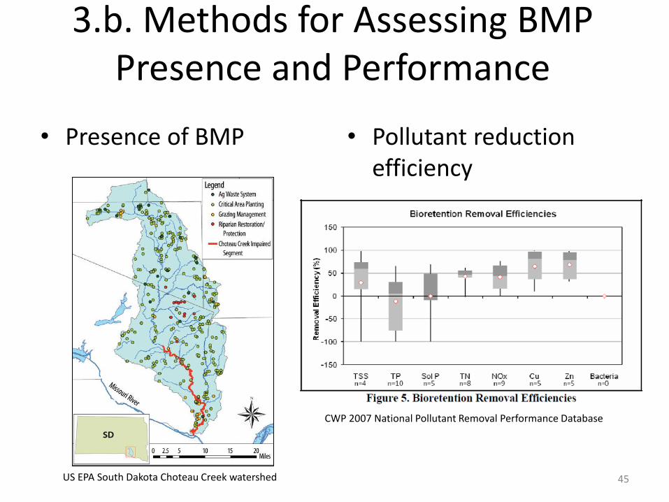
• Presence of BMP • Pollutant reduction efficiency

45

CWP 2007 National Pollutant Removal Performance Database

US EPA South Dakota Choteau Creek watershed

3.b. Methods for Assessing BMP Presence and Performance

• Direct measurements

– Soil tests

– On-site inspection

– Remote sensing

• Indirect methods

– Landowner self-reporting

– Third-party surveys

46

Different types of BMPs require different verification methods

No single approach is likely to provide all the information needed

3.b. Methods for Assessing BMP Presence and Performance

Need to search BMP information sources for complete record of BMPs already on the ground during the project planning phase

– Permit records

– Agency programs; cost-share records

– Voluntary implementation

47

3.b. Methods for Assessing BMP Presence and Performance

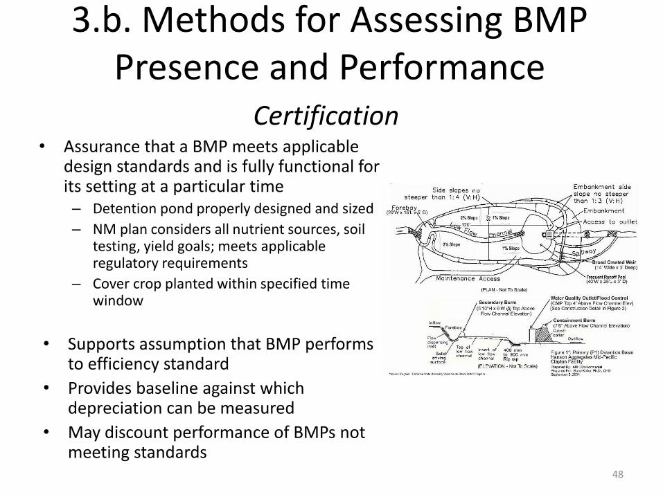
• Assurance that a BMP meets applicable design standards and is fully functional for its setting at a particular time – Detention pond properly designed and sized

– NM plan considers all nutrient sources, soil testing, yield goals; meets applicable regulatory requirements

– Cover crop planted within specified time window

• Supports assumption that BMP performs to efficiency standard

• Provides baseline against which depreciation can be measured

• May discount performance of BMPs not meeting standards

48

3.b. Methods for Assessing BMP Presence and Performance

Certification

49

3.b. Methods for Assessing BMP Presence and Performance

Certification

50

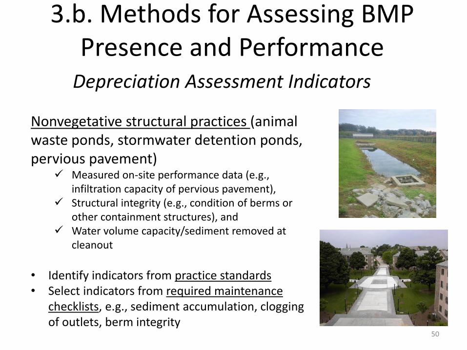
Nonvegetative structural practices (animal waste ponds, stormwater detention ponds, pervious pavement)

Measured on-site performance data (e.g., infiltration capacity of pervious pavement),

Structural integrity (e.g., condition of berms or other containment structures), and

Water volume capacity/sediment removed at cleanout

• Identify indicators from practice standards • Select indicators from required maintenance

checklists, e.g., sediment accumulation, clogging of outlets, berm integrity

3.b. Methods for Assessing BMP Presence and Performance

Depreciation Assessment Indicators

51

Vegetative structural practices (constructed

wetlands, swales, rain gardens, riparian buffers, and filter strips) Extent and health of vegetation (e.g.,

measurements of soil cover or plant density), Quality of overland flow filtering (e.g., evidence of

short-circuiting by concentrated flow or gullies through buffers or filter strips),

On-site capacity testing of rain gardens using infiltrometers or similar devices,

Visual observations (e.g., presence of water in swales and rain gardens).

3.b. Methods for Assessing BMP Presence and Performance

Depreciation Assessment Indicators

52

Nonstructural vegetative practices (e.g., cover crops, reforestation) Density of cover crop planting (e.g., plant count), Percent of area covered by cover crop, Extent and vitality of tree seedlings.

3.b. Methods for Assessing BMP Presence and Performance

Depreciation Assessment Indicators

53

Management practices (e.g., nutrient management, conservation tillage, street sweeping) Records of street sweeping frequency and mass of

material collected, Area or percent of cropland under conservation tillage, Extent of crop residue coverage on conservation tillage

cropland, and Fertilizer and/or manure application rates and

schedules, crop yields, soil test data, plant tissue test results, and fall residual nitrate tests.

3.b. Methods for Assessing BMP Presence and Performance

Depreciation Assessment Indicators

Others Sources of Assessment Methods

• Gulliver, J.S., A.J. Erickson, and P.T. Weiss (editors). 2010. "Stormwater Treatment: Assessment and Maintenance." University of Minnesota, St. Anthony Falls Laboratory. Minneapolis, MN. http://stormwaterbook.safl.umn.edu/

• Chesapeake Bay Verification Resources

54

3.c. Data Analysis and Presentation

• Data on indicators can be expressed and analyzed in several ways, depending on the nature of the indicators used

• For continuous numerical data, report either in raw form (e.g., acres with 30% or more residue cover) or as a percentage (e.g., percent of crop acres with 30% or more residue cover) – cover crop or conservation tillage acreage – manure application rates – miles of street sweeping – mass of material removed from catch basins or detention

ponds – acres of logging roads/landings

55

• Categorical data are more difficult to express quantitatively. – Maintenance of detention basin ridge height and

outlet elevations – Condition of berms or terraces – Observations of water accumulation and flow

• It might be necessary to establish an ordinal scale (e.g., condition rated on a scale of 1–10) or a binary yes/no condition, then use best professional judgment to assess influence on BMP performance

56

3.c. Data Analysis and Presentation

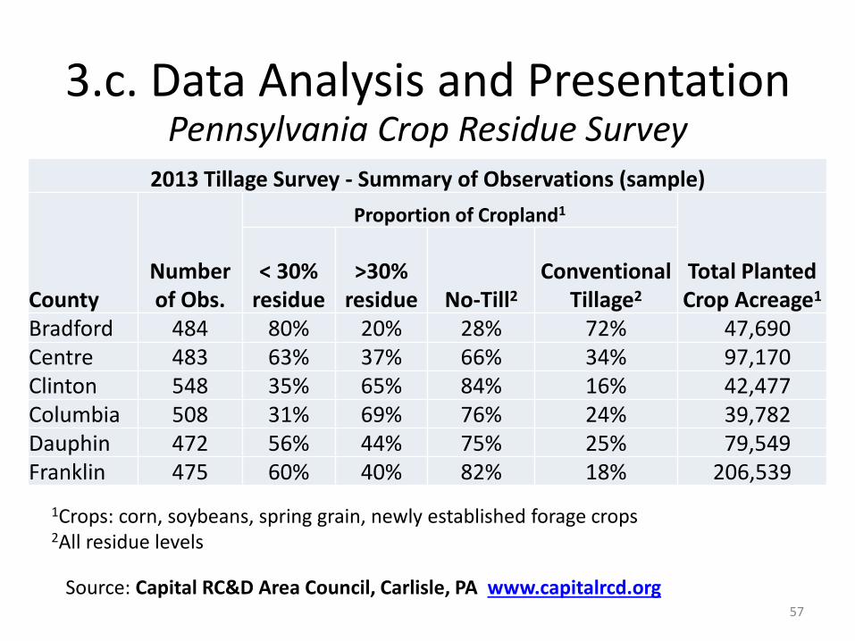
Pennsylvania Crop Residue Survey 2013 Tillage Survey - Summary of Observations (sample)

County Number of Obs.

Proportion of Cropland1

Total Planted Crop Acreage1

< 30% residue

>30% residue No-Till2

Conventional Tillage2

Bradford 484 80% 20% 28% 72% 47,690 Centre 483 63% 37% 66% 34% 97,170 Clinton 548 35% 65% 84% 16% 42,477 Columbia 508 31% 69% 76% 24% 39,782 Dauphin 472 56% 44% 75% 25% 79,549 Franklin 475 60% 40% 82% 18% 206,539

57

1Crops: corn, soybeans, spring grain, newly established forage crops 2All residue levels

Source: Capital RC&D Area Council, Carlisle, PA www.capitalrcd.org

3.c. Data Analysis and Presentation

Maryland Nutrient Management Program

• 733 on-farm audits (14% of regulated farms)

• Verify NMP is current, examine records for consistency with plan

• Follow-up visits showed 66% compliance

• Enforcement actions for others

58

2014 Annual Report

Source: Maryland Department of Agriculture http://mda.maryland.gov/resource_conservation/counties/MDANMPAnnual2014.pdf

3.c. Data Analysis and Presentation

BMP Performance Curves

• In some cases, it might be possible to use modeling or other quantitative analysis to estimate individual or watershed-level BMP performance levels based on verification data. – E.g., Tetra Tech (2010) presented a series of BMP

performance curves based on monitoring and modeling data that relate pollutant removal efficiency to depth of runoff treated (next slide). Where depreciation indicators track changes in depth of runoff treated as the capacity of a BMP decreases (e.g., from sedimentation), resulting changes in pollutant removal could be estimated from a performance curve.

59

3.c. Data Analysis and Presentation

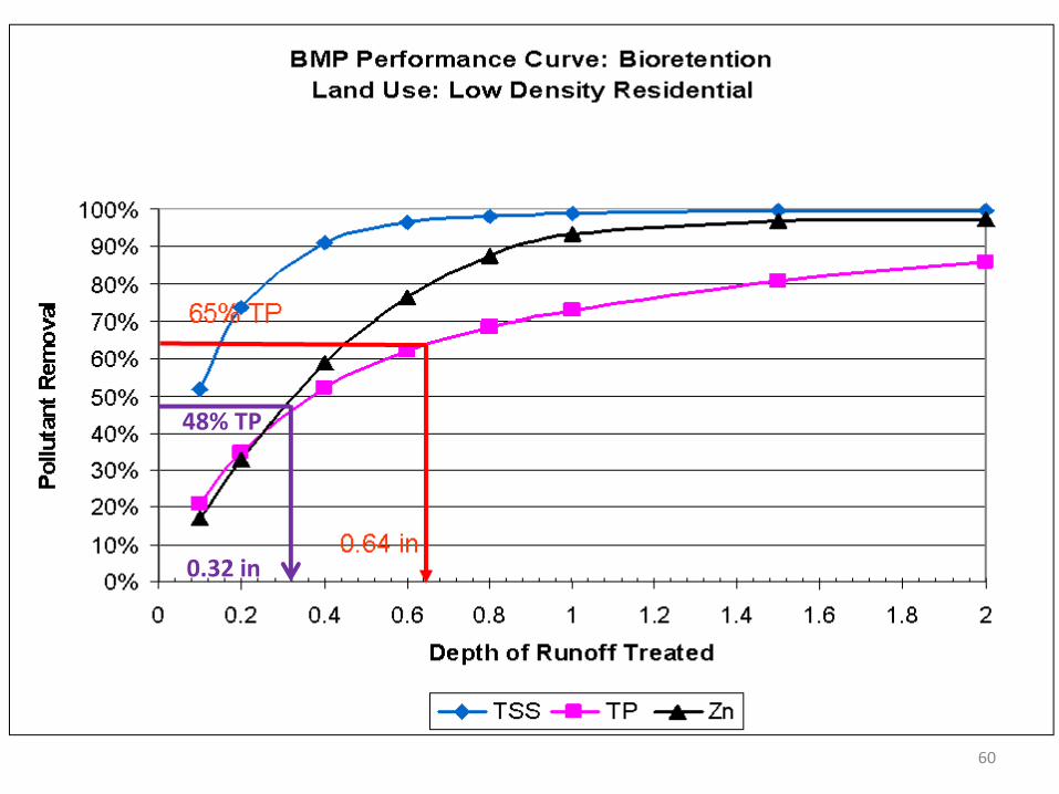
0.32 in

48% TP

60

4. Adjusting for Depreciation

• Information on BMP depreciation can be used to improve both project management and project evaluation

61

4.a. Project Planning & Management

• Establish baseline conditions using adjustments based on knowledge of BMP depreciation or growth stage of vegetative practices.

• Adjust treatment plan to reflect current condition of existing BMPs.

– Alternative BMPs or different level of treatment

– Incorporate repair or enhanced maintenance and operation of existing BMPs

62

• Track both traditional measures of BMP implementation and indicators of BMP depreciation to provide holistic progress assessments that measure implementation as well as maintenance, and operation of BMPs.

• Examine patterns in BMP depreciation for information on systematic failures in BMP design or management that can be addressed through changes to standards and specifications, contract terms, or permit requirements.

63

4.a. Project Planning & Management

64

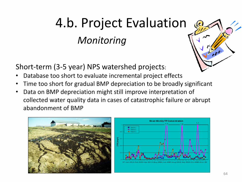
Short-term (3-5 year) NPS watershed projects:

• Database too short to evaluate incremental project effects • Time too short for gradual BMP depreciation to be broadly significant • Data on BMP depreciation might still improve interpretation of

collected water quality data in cases of catastrophic failure or abrupt abandonment of BMP

0 7 -Ja n -9 9 1 8 -Fe b -9 9 0 1 -A p r-9 9 1 3 -M a y -9 92 4 -Ju n -9 90 5 -A u g -9 91 6 -S e p -9 92 8 -O c t-9 90 9 -D e c -9 9

0

0.2

0.4

0.6

0.8

1

[TP

] (m

g/l

)

Station 1

Station 2

Station 3

Mean Weekly TP Concentration

1.24 1.021.13

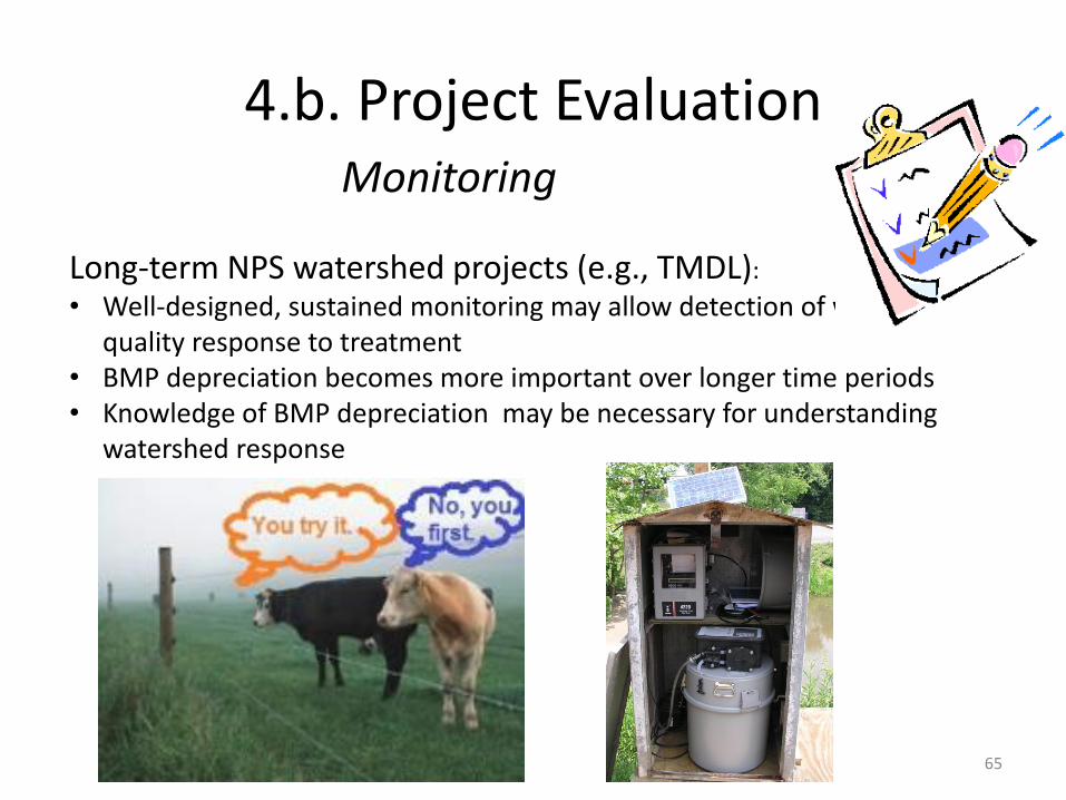
4.b. Project Evaluation Monitoring

65

Long-term NPS watershed projects (e.g., TMDL):

• Well-designed, sustained monitoring may allow detection of water quality response to treatment

• BMP depreciation becomes more important over longer time periods • Knowledge of BMP depreciation may be necessary for understanding

watershed response

4.b. Project Evaluation Monitoring

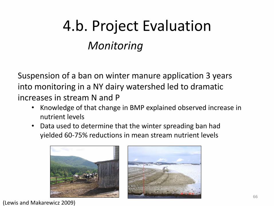
Suspension of a ban on winter manure application 3 years into monitoring in a NY dairy watershed led to dramatic increases in stream N and P

• Knowledge of that change in BMP explained observed increase in nutrient levels

• Data used to determine that the winter spreading ban had yielded 60-75% reductions in mean stream nutrient levels

66

(Lewis and Makarewicz 2009)

Monitoring

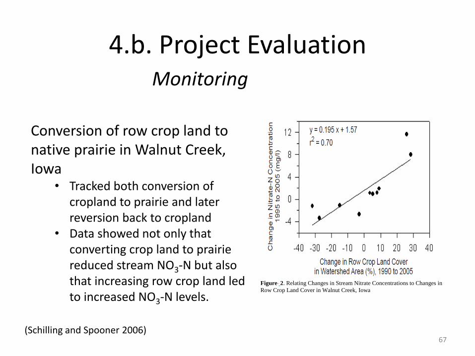
4.b. Project Evaluation

67

Conversion of row crop land to native prairie in Walnut Creek, Iowa

• Tracked both conversion of cropland to prairie and later reversion back to cropland

• Data showed not only that converting crop land to prairie reduced stream NO3-N but also that increasing row crop land led to increased NO3-N levels.

Figure 2. Relating Changes in Stream Nitrate Concentrations to Changes in

Row Crop Land Cover in Walnut Creek, Iowa

(Schilling and Spooner 2006)

4.b. Project Evaluation Monitoring

Knowledge of BMP depreciation should be part of model inputs and parameterization. • The magnitude of implementation (e.g., acres of treatment)

and the spatial distribution of both annual and structural BMPs should be part of model input and should not be static parameters.

– Adjust BMP pollutant reduction efficiencies based on verification of land treatment performance levels in the watershed

– Perhaps set up a tiered approach for BMP efficiencies (e.g., different efficiency values for BMPs determined to be in fair, good, or excellent condition)

• In the planning phase of a watershed project, multiple scenarios could be modeled to reflect the potential range of performance levels for BMPs already in place.

68

4.b. Project Evaluation Modeling

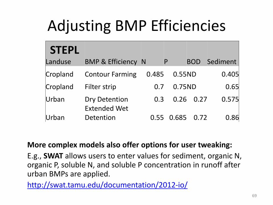
Adjusting BMP Efficiencies

Landuse BMP & Efficiency N P BOD Sediment

Cropland Contour Farming 0.485 0.55 ND 0.405

Cropland Filter strip 0.7 0.75 ND 0.65

Urban Dry Detention 0.3 0.26 0.27 0.575

Urban Extended Wet Detention 0.55 0.685 0.72 0.86

69

STEPL

More complex models also offer options for user tweaking:

E.g., SWAT allows users to enter values for sediment, organic N, organic P, soluble N, and soluble P concentration in runoff after urban BMPs are applied.

http://swat.tamu.edu/documentation/2012-io/

5. Recommendations

The importance of accurate knowledge of BMP depreciation varies across projects and during the lifetime of a single project. • During the planning phase, when planning for the achievement of

pollutant reduction targets relies heavily on existing BMPs, good information on performance of existing BMPs is essential.

• If existing BMPs are a trivial part of the overall watershed plan, knowledge of BMP depreciation might not be critical during planning.

• As projects move forward, depreciation of existing and new BMPs becomes important; the types of BMPs implemented, their relative costs and contributions to achievement of project pollutant reduction goals, and the likelihood that BMP depreciation will occur will largely determine the type and extent of BMP verification required over time.

70

.

• During project planning, collect accurate and complete information about: – Land use, – Land management, and – The implementation and operation of existing BMPs for

characterization of overall baseline NPS loads, better identification of critical source areas, and effective prioritization of new land treatment. This information should include:

• Original BMP installation dates, • Design specifications of individual BMPs, • Data on BMP performance levels if available, and • The spatial distribution of BMPs across the watershed.

71

5. Recommendations

• Track the factors that influence BMP depreciation in the watershed, including:

– Variations in weather that influence BMP performance,

– Changes in land use, land ownership, and land management,

– Inspection and enforcement activities on permitted practices, and

– Operation, maintenance, and management of implemented practices.

72

5. Recommendations

• Develop and use observable indicators of BMP status/performance that:

– Are tailored to the set of BMPs implemented in the watershed and practical within the scope of the watershed project’s resources,

– Can be quantified or scaled to document the extent and magnitude of treatment depreciation, and

– Are able to be paired with water quality monitoring data.

73

5. Recommendations

• After the implementation phase of the NPS project, conduct verification activities to document the continued existence and function of implemented practices to assess the magnitude of depreciation and provide a basis for corrective action. The verification program should: – Identify and locate all BMPs of interest, including cost-

shared, non cost-shared, required, and voluntary practices, – Capture information on structural, annual, and

management BMPs, – Obtain data on BMP operation and maintenance activities,

and – Include assessment of data accuracy and confidence.

74

5. Recommendations

• To adjust for depreciation of land treatment, apply verification data to watershed project management and evaluation by: – Applying results directly to permit compliance programs,

– Relating documented changes in land treatment performance levels to observed water quality,

– Incorporating measures of depreciated BMP effectiveness into modeling efforts, and

– Using knowledge of treatment depreciation to correct problems and target additional practices as necessary to meet project goals in an adaptive watershed management approach.

75

5. Recommendations

Baker, D.B. 2010. Trends in Bioavailable Phosphorus Loading to Lake Erie. Final Report. LEPF Grant 315-07. Prepared for the Ohio Lake Erie Commission by the National Center for Water Quality Research, Heidelberg University, Tiffin, OH. http://141.139.110.110/sites/default/files/jfuller/images/13%20Final%20Report,%20LEPF%20Bioavailability%20Study.pdf. Dosskey, M.G., M. J. Helmers, D.E. Eisenhauer, T.G. Franti, and K.D. Hoagland. 2002. Assessment of concentrated flow through riparian buffers. Journal of Soil and Water Conservation 57(6):336–343. Hill, R.P. 1996. Procedures for cropland transect surveys for obtaining reliable county- and watershed-level tillage, crop residue, and soil loss data. Core4: Conservation for Agriculture’s Future, Conservation Technology Information Center, West Lafayette, IN. http://www2.ctic.purdue.edu/Core4/CT/transect/Transect.html (Accessed October 13, 2015). Jackson-Smith, D.B., M. Halling, E. de la Hoz, J.P. McEvoy, and J.S. Horsburgh. 2010. Measuring conservation program best management practice implementation and maintenance at the watershed scale. Journal of Soil and Water Conservation 65(6):413–423. Joosse, P. J., and D.B. Baker. 2011. Context for re-evaluating agricultural source phosphorus loadings to the Great Lakes. Canadian Journal of Soil Science 91:317–327. Lewis, T.W., and J.C. Makarewicz. 2009. Winter application of manure on an agricultural watershed and its impact on downstream nutrient fluxes. Journal of Great Lakes Research 35(sp1):43–49. 76

References

Lindsey, G., L. Roberts, and W. Page. 1992. Maintenance of stormwater BMPs in four Maryland counties: A status report. Journal of Soil and Water Conservation 47(5):417–422. Schilling, K.E., and J. Spooner. 2006. Effects of watershed-scale land use change on stream nitrate concentrations. Journal of Environmental Quality 35:2132–2145. Tetra Tech, Inc. 2010. Stormwater Best Management Practices (BMP) Performance Analysis. Prepared for U.S. Environmental Protection Agency Region 1 by Tetra Tech, Inc., Fairfax, VA. Revised March2010; accessed April 24, 2015. http://www.epa.gov/region1/npdes/stormwater/assets/pdfs/BMP-Performance-Analysis-Report.pdf. Tortora, R.D. 1978. A note on sample size estimation for multinomial populations. The American Statistician, 32(3):100-102. Urbonas, B., and J. Wulliman. 2007. Stormwater Runoff Control Using Full Spectrum Detention. In Proceedings of World Environmental and Water Resources Congress 2007: Restoring Our Natural Habitat, American Society of Civil Engineers. http://cedb.asce.org/cgi/WWWdisplay.cgi?159418. USEPA. 2008. Handbook for Developing Watershed Plans to Restore and Protect Our Waters. EPA 841-B-08-002. http://water.epa.gov/polwaste/nps/upload/2008_04_18_NPS_watershed_handbook_handbook-2.pdf. USEPA. 2013. Nonpoint Source Program and Grants Guidelines for States and Territories. http://water.epa.gov/polwaste/nps/upload/319-guidelines-fy14.pdf. Virginia Department of Conservation and Recreation. 1999. Virginia Stormwater Management Handbook. Division of Soil and Water Conservation, Richmond, VA . http://www.deq.virginia.gov/Programs/Water/StormwaterManagement/Publications.aspx.

77