BNL- 65605 Informal Report Results of Stretched Wire Field Integral Measurements on the Mini-Undulator Magnet - Comparison of Results Obtained from Circular and Translational Motion of the Integrating Wire Lorraine Solomon May 1998 National Synchrotron Light Source Brookhaven National Laboratory, Upton,NY 11973 USA Work performed under the auspices of the U.S. Department of Energy, under contract DE-AC02-9 8 CH 1 08 8 6
Transcript
BNL- 65605 Informal Report
Results of Stretched Wire Field Integral Measurements on the Mini-Undulator Magnet - Comparison of Results Obtained from
Circular and Translational Motion of the Integrating Wire
Lorraine Solomon
May 1998
National Synchrotron Light Source Brookhaven National Laboratory,
Upton,NY 11973 USA
Work performed under the auspices of the U.S. Department of Energy, under contract DE-AC02-9 8 CH 1 08 8 6
DISCLAIMER
"hiis report was prepared as an account of work sponsored by an ageng of the United States Government. Neither the United States Government nor any agency thereof, nor any of their employees, make any warranty, express or implied, or a~sumes any legal iiabili- ty or responn'bility for the accuracy, completeness, or usefulness of any information, appa- ratus, product, or proces disdased, or represents ihat its use would not infringe privately owned rights Reference herein to any specific commercial product, p m a s , or service by trade name, trademark, manufacturer, or otfiemise does not necessafily constitute or imply its endorsement, r e c o d t i o n , or favoring by the United States Government or any agency thereof. The views and opinions of autfiors expressed herein do not necersar- ily state or reflect those of the United States Goverrpent or any agency thereof.
DISCLAIMER
Portions of this document may be illegible electronic image products. Images are produced from the best available original document.
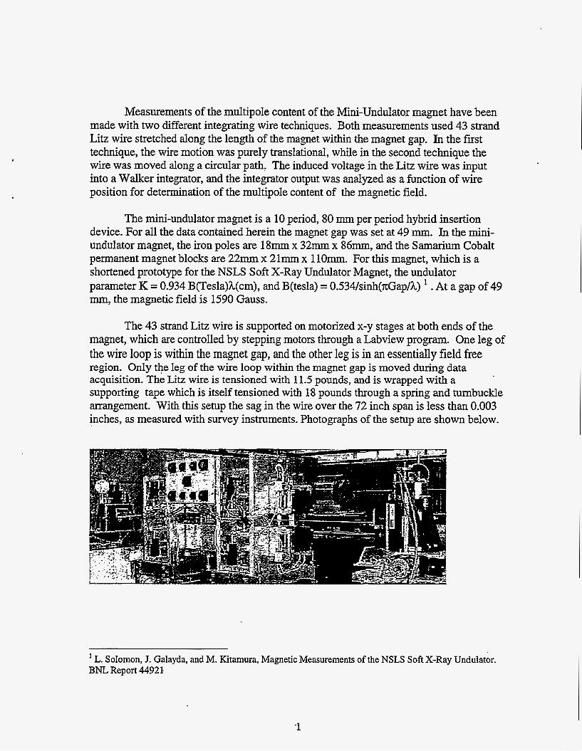
Measurements of the multipole content of the Mini-Undulator magnet have been made with two different integrating wire techniques. Both measurements used 43 strand Litz wire stretched along the length of the magnet within the magnet gap. In the first technique, the wire motion was purely translational, while in the second technique the wire was moved along a circular path, The induced voltage in the Litz wire was input into a Walker integrator, and the integrator output was analyzed as a function of wire position for determination of the multipole content of the magnetic field.
The mini-undulator magnet is a 10 period, 80 mm per period hybrid insertion device. For all the data contained herein the magnet gap was set at 49 mm. In the mini- undulator magnet, the iron poles are 18mm x 32mm x 86mm, and the Samarium Cobalt permanent magnet blocks are 22mm x 21mm x 110mm. For this magnet, which is a shortened prototype for the NSLS Soft X-Ray Undulator Magnet, the undulator parameter K = 0.934 B(Tesla)h(cm), and B(tes1a) = 0.534/sinh(.nGap/h) * . At a gap of 49 mm, the magnetic field is 1590 Gauss.
The 43 strand Litz wire is supported on motorized x-y stages at both ends of the magnet, which are controlled by stepping motors through a Labview program. One leg of the wire loop is within the magnet gap, and the other leg is in an essentially field free region. Only the leg of the wire loop within the magnet gap is moved during data acquisition. The Litz wire is tensioned with 11.5 pounds, and is wrapped with a supporting tape which is itself tensioned with 18 pounds through a spring and turnbuckle arrangement. With this setup the sag in the wire over the 72 inch span is less than 0.003 inches, as measured with survey instruments. Photographs of the setup are shown below.
L. Solomon, J. Galayda, and M. Kitamura, Magnetic Measurements of the NSLS Soft X-Ray Undulator. BNL Report 44921
-1
The Litz wire within the magnet gap is moved, and the induced voltage due to the change in the flux intercepted by the coil is input into a Walker integrator. The induced voltage in the coil is related to the change in the magnetic flux enclosed by the coil through the following
I Voltage dt [v-sec] = N, * Ax [m] * I B[T] dl[m] (1)
where N, is the number of turns in the coil, and Ax is the distance moved by the coil. In the Walker integrator, the front panel reading is
Front panel reading [ 10” T m’] =
where N = the thumbwheel setting on the integrator, and D = the decade setting on the integrator.
I Voltage dt [v-secl N D
Combining the two above equations, one gets that
I B dl [G cm] = Front panel reading * N * D * lo3 N, *Ax[cm]
(3)
where Ax is in cm. This form is useful for analysis of translational motion of the Litz wire.
2
Circular Wire Motion
In the case where the wire motion was circular, the wire was moved along circles with radii 2mm, 7mm, 12mm, 17m, 2 0 m , and 24mm. During these scans there were only 34 functioning coil loops within the Litz wire. For these scans, the front panel integrator thumbwheel was set to N = Nt *r[mm] Le., N= 68,238,408,578,680, and 816 respectively, and D=10. With these settings, the integrated voltages for the various scans were similar even though the path length through which the wire moved differed (eq. [3]). The wire motion was stopped at 16 points along the circle (i.e. at intervals of 22.5 degrees) and integrator data was obtained. Therefore, the arc length between two adjacent data points varied from 0.8mm to 9.4 nun as the circle radius increased from 2mm to 24 mm, with a concurrent increase in induced wire voltage. Integrator data was taken for motion from a starting wire position to the next wire position, and then also for wire motion back to the starting wire position. The actual integrator signal was taken as half the difference between the two integrator readings, which assumes a linear integrator drift with time. This process was repeated 20 times for each position of the wire, and then averaged to obtain a single data point used in the field analysis. That is, each data point at a given angle is representative of the average of 20 linear drift compensated data points, and 16 data points (Le. averaged data at 16 angles) are used in the multipole analysis. For this analysis the field is expressed in terms of radial coordinates r and 8,
B, (r,e) = c[ancos(nO) + bnsin(n8)] f -' (4)
' SV (r,e) dt = Nt jdz jB,rd8 (5)
where the limits of integration on t are tI(81) + t,(0,), on z are -L/2+ U2, and on 8 are . Integrating over 8,
where An = I a, dz , Bn = .I bn dz, A0 = 81432 and 8 = { 01+02}/2.
Fitting the integrator output to a function of the form
I V dt = V1,sjn sin k0+ V2,sinsin 2ke + V3,sin sin 3k8+ Vl,cosCOSke + V2,cos~~~2k8 + V3,cos~~~3k8
where k=2n/36Oo, and 8 is the angular position of the wire, gives the relationship that
Zangrando, D. and Walker, R.P. A Stretched Wire System for Accurate Integrated Magnetic Field Measurements in Insertion Devices, NIM Volume 376 N0.2 p.275 (1996)
3
(7)
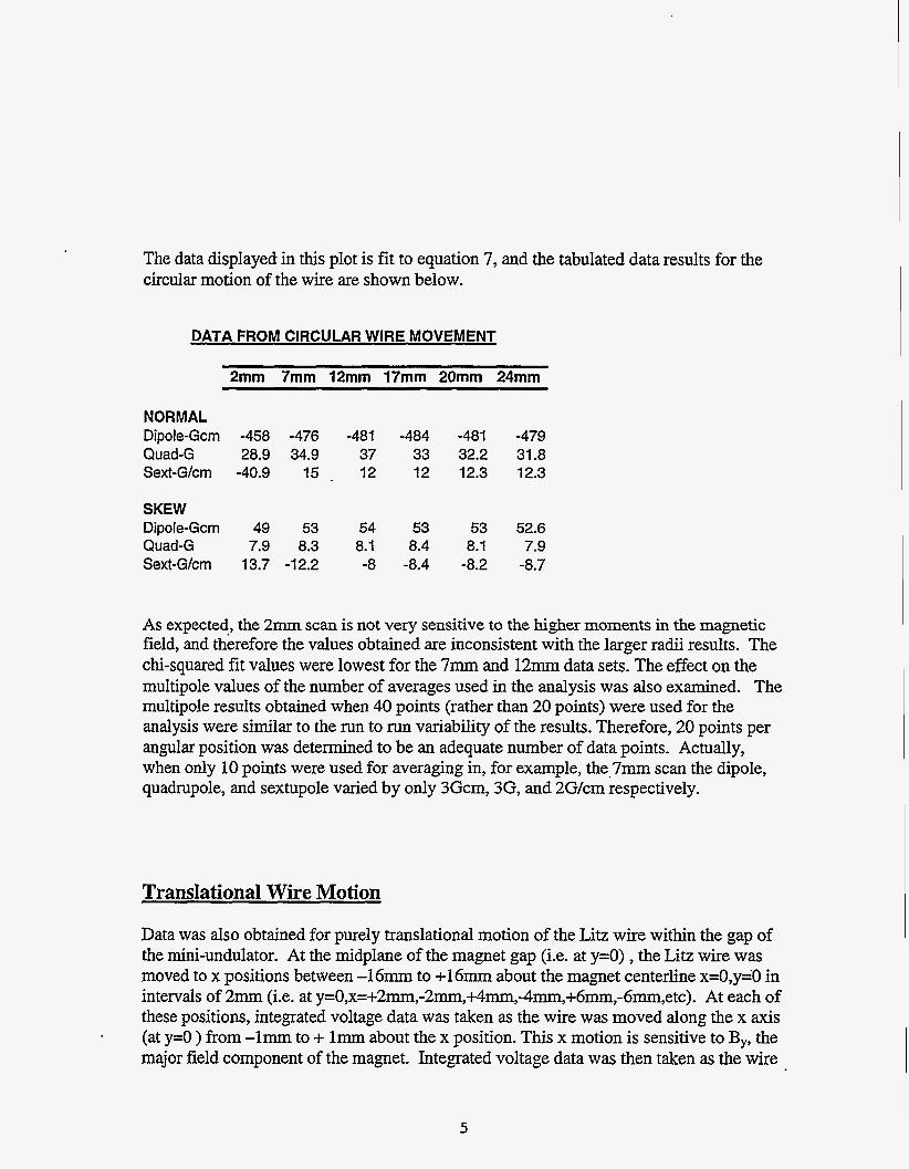
The data displayed in this plot is fit to equation 7, and the tabulated data results for the circular motion of the wire are shown below.
As expected, the 2mm scan is not very sensitive to the higher moments in the mapetic field, and therefore the values obtained are inconsistent with the larger radii results. The chi-squared fit values were lowest for the 7mm and 12mm data sets. The effect on the multipole values of the number of averages used in the analysis was also examined. The multipole results obtained when 40 points (rather than 20 points) were used for the analysis were similar to the run to run variability of the results. Therefore, 20 points per angular position was determined to be an adequate number of data points. Actually, when only 10 points were used for averaging in, for example, the 7mm scan the dipole, quadrupole, and sextupole varied by only 3Gcm, 3G, and 2Gkm respectively.
Translational Wire Motion
Data was also obtained for purely translational motion of the Litz wire within the gap of the mini-undulator. At the midplane of the magnet gap (i.e. at y=O) , the Litz wire was moved to x positions between -16mm to +16mm about the magnet centerline x=O,y=O in intervals of 2mm (Le. at y=0,x=+2mm,-2mm,+4mm,-4mm,+6mm7-6mm7etc). At each of these positions, integrated voltage data was taken as the wire was moved along the x axis (at y=O ) from -1mm to + lmm about the x position. This x motion is sensitive to By, the major field component of the magnet. Integrated voltage data was then taken as the wire
5
was moved from y=+lmrn to y=-lmm at each x position. This y motion is sensitive to Bx, the skew field component. The motion was repeated 20 times and the data was collected and averaged, resulting in the following data shown in both tabular and graphic form.
6
Translational Wire Motion
l8 T
E !2
10
'\
I n Y . I
-20 -1 5 -1 0 -5 0 5 10 15 20 Position (mm)
In this plot, the darker diamonds represent the Y scan results (i.e. the B, field) and the lighter boxes represent the X scan results (i.e. the By field). The x-motion results, i.e. the By integrals, have been reduced by a constant value of 35 Gcm in the graph to enable both the normal and the skew fields to be seen clearly on the same graph.
This data is analyzed for multipole content by fitting the data to a power series of the form
J V dt = Bo+ Blx+ B2x2
where Bo is the dipole field, B1 is the integrated quadrupole, and B2 is the integrated sextupole. This functional form was applied to the data over various restricted ranges. In order to compare the multipole results from the translational wire motion to the circular wire motion, the range was restricted to +/- 2mm, +/- 8mm, +/- 12mm, and +/-17mm, which includes 3,9,1l,and 17 data points respectively.
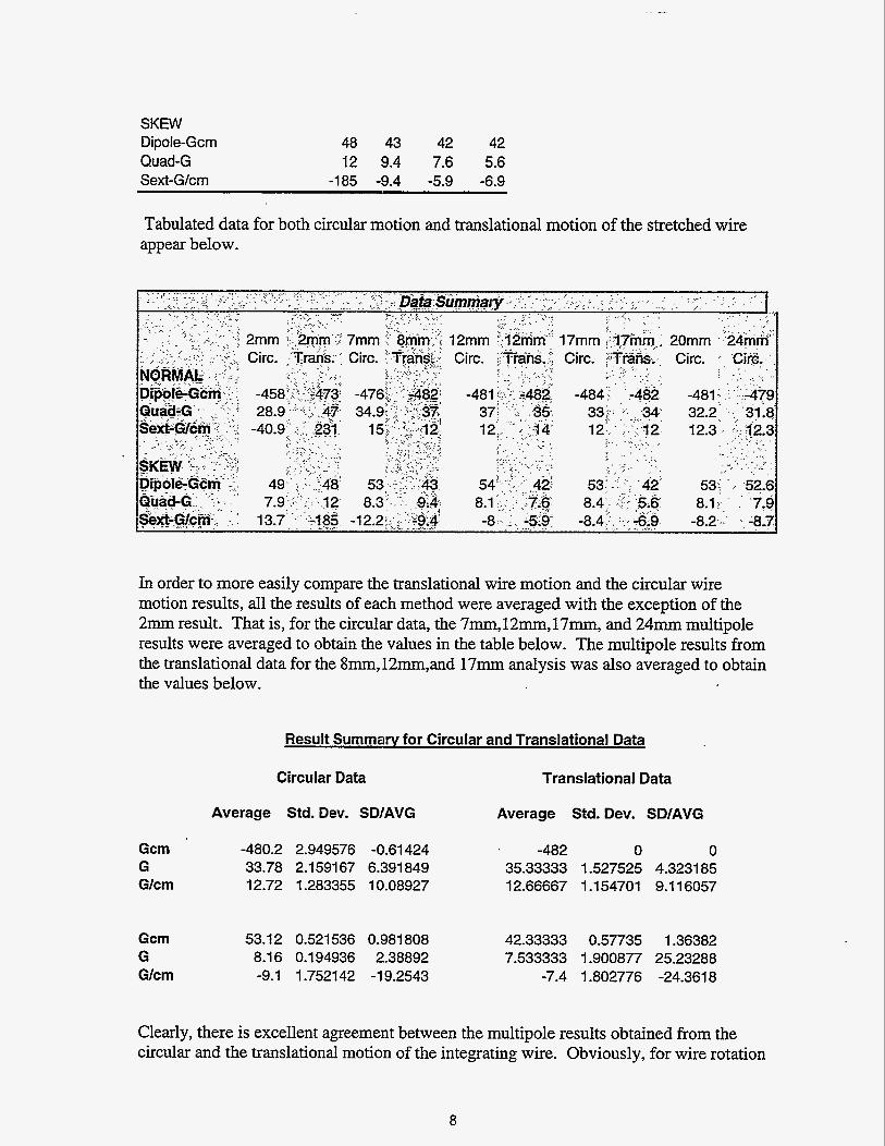
Tabulated data for both circular motion and translational motion of the stretched wire appear below.
-~
In order to more easily compare the translational wire motion and the circular wire motion results, all the results of each method were averaged with the exception of the 2mm result. That is, for the circular data, the 7mm,12mm,17mm7 and 24mm multipole results were averaged to obtain the values in the table below. The multipole results from the translational data for the 8mm,12mm,and 17mm analysis was also averaged to obtain the values below.
Gcrn G G/cm
Gcrn G G/cm
Result Summarv for Circular and Translational Data
Clearly, there is excellent agreement between the multipole results obtained from the circular and the translational motion of the integrating wire. Obviously, for wire rotation
8
at small radii, there is little sensitivity to higher multipoles in the magnetic field. However, both circular and translational motion of the integrating wire at positions of approximately one-third of the magnet half gap was sufficient to determine the multipoles. That is, data at 7mm and 8mm with a magnet gap of 49 mm was sufficient to determine the multipole content of the magnet, while data at only 2mm was clearly not adequate. The translational scans required to obtain the multipoles take about twice as long (i.e. about 2 hours) to complete as the circular motion scans, because in the former case two orthogonal motions are required to determine the normal and skew fields.