JSS Journal of Statistical Software November 2007, Volume 21, Issue 11. http://www.jstatsoft.org/ boa: An R Package for MCMC Output Convergence Assessment and Posterior Inference Brian J. Smith The University of Iowa Abstract Markov chain Monte Carlo (MCMC) is the most widely used method of estimating joint posterior distributions in Bayesian analysis. The idea of MCMC is to iteratively produce parameter values that are representative samples from the joint posterior. Unlike frequentist analysis where iterative model fitting routines are monitored for convergence to a single point, MCMC output is monitored for convergence to a distribution. Thus, specialized diagnostic tools are needed in the Bayesian setting. To this end, the R package boa was created. This manuscript presents the user’s manual for boa, which outlines the use of and methodology upon which the software is based. Included is a description of the menu system, data management capabilities, and statistical/graphical methods for convergence assessment and posterior inference. Throughout the manual, a linear regression example is used to illustrate the software. Keywords : Bayesian analysis, convergence diagnostics, Markov chain Monte Carlo, posterior inference, R. 1. Introduction In frequentist-based statistical modeling, estimated parameters and associated standard errors are sought. Such estimates might be the limit of a sequence of parameter values generated via iterative computational routines. In that setting, convergence assessment involves check- ing that the sequence has converged to a single point. In Bayesian modeling, interest lies in estimating posterior distributions of model parameters rather than individual parameter values and asymptotic standard errors. Nevertheless, iterative computational algorithms may still be used to produce a sequence of parameter values. However, in the Bayesian setting, convergence assessment involves checking that the sequence, or chain, has converged to and provides a representative sample from the posterior distribution.
Markov chain Monte Carlo (MCMC) is the most widely used method of estimatingjoint posterior distributions in Bayesian analysis. The idea of MCMC is to iterativelyproduce parameter values that are representative samples from the joint posterior. Unlikefrequentist analysis where iterative model fitting routines are monitored for convergenceto a single point, MCMC output is monitored for convergence to a distribution. Thus,specialized diagnostic tools are needed in the Bayesian setting. To this end, the R packageboa was created. This manuscript presents the user’s manual for boa, which outlinesthe use of and methodology upon which the software is based. Included is a descriptionof the menu system, data management capabilities, and statistical/graphical methodsfor convergence assessment and posterior inference. Throughout the manual, a linearregression example is used to illustrate the software.
Keywords: Bayesian analysis, convergence diagnostics, Markov chain Monte Carlo, posteriorinference, R.
1. Introduction
In frequentist-based statistical modeling, estimated parameters and associated standard errorsare sought. Such estimates might be the limit of a sequence of parameter values generatedvia iterative computational routines. In that setting, convergence assessment involves check-ing that the sequence has converged to a single point. In Bayesian modeling, interest liesin estimating posterior distributions of model parameters rather than individual parametervalues and asymptotic standard errors. Nevertheless, iterative computational algorithms maystill be used to produce a sequence of parameter values. However, in the Bayesian setting,convergence assessment involves checking that the sequence, or chain, has converged to andprovides a representative sample from the posterior distribution.
2 boa: MCMC Output Convergence Assessment and Posterior Inference in R
Markov chain Monte Carlo (MCMC) is a powerful and widely used method for iterativelysampling from posterior distributions. Metropolis-Hastings sampling is one MCMC methodthat can be utilized to generate draws, in turn, from full conditional distributions of modelparameters (Hastings 1970). Several other algorithmic approaches are available, such asGibbs, slice (Neal 2003), and adaptive rejection sampling (Gilks and Wild 1992). Addi-tional implementation choices involve the decision to use a compiled language, such as C;an interpreted language, such as R (R Development Core Team 2006); or existing software.Programming of the algorithms directly requires (1) derivation of posterior full conditionalsfor all model parameters — at least up to constants of proportionality; (2) familiarity withvarious MCMC sampling techniques; and (3) scientific computing proficiency. Alternatively, awide range of Bayesian models can be fit with available software programs, such as WinBUGS(Thomas, Best, and Spiegelhalter 2000) or its open-source counterpart OpenBUGS (Thomas,O’Hara, Ligges, and Sturtz 2006), that have built-in algorithms for MCMC sampling. Forsuch programs, the user provides a model specification without needing to worry about theimplementation of the MCMC algorithm. Advantages of the programming approach includeapplicability to a wider range of models and greater control over the sampling techniquesused in the MCMC implementation. The potentially significant trade-off is the increaseddevelopment time added to the analysis, relative to the use of available software.
Whether the choice is to implement an MCMC algorithm directly or to rely on available soft-ware, the goal is to obtain chains of parameter values that are representative samples fromthe joint posterior distribution. This manuscript describes the R package boa designed forconvergence assessment and posterior inference of MCMC output. Development of boa beganin 2000 as a complete re-write of the functions and user-interface supplied by the CODA soft-ware of Best, Cowles, and Vines (1995). boa is designed for use from the supplied menu-driveninterface which has been designed to make the learning curve low for R novices. Consequently,R programming proficiency is not a prerequisite for the package’s use. Plummer, Best, Cowles,and Vines subsequently developed the R package coda mirroring the functionality of CODAand boa and providing command-line access to its diagnostic functions. The object-orientedlibrary of functions provided by coda appeals to experienced R programmers interested inincorporating convergence diagnostics into their own programs. A description of coda andsynopsis of the history and redesign of CODA can be found in Plummer et al. (2006). In thesections that follow, the user’s manual for boa is presented along with examples of its use andthe methodology upon which the software is based.
2. Bayesian output analysis program (boa)
boa is a program for carrying out convergence diagnostics and statistical and graphical analysisof Monte Carlo sampling output. It can be used as a post-processor for the WinBUGS softwareor for any other program that produces sampling output.
2.1. Program installation
boa is available as an open-source package for the R system for statistical computing. Thepackage is publicly available from the Comprehensive R Archive Network at http://CRAN.R-project.org/. Hence, on computers connected to the internet, boa can be downloadedand installed automatically by entering the following at the R command line:
Thereafter, the supplied functions can be used by loading the package into R with the com-mand
R> library("boa")
2.2. Linear regression example data
Example MCMC output is included with the boa package. The output comes from a simplelinear regression example that appears in the BUGS 0.5 manual (Spiegelhalter, Thomas, Best,and Gilks 1996). The example presents a regression analysis of (x, y) observations (1, 1), (2,3), (3, 3), (4, 3), and (5, 5) performed with the following Bayesian model:
yi ∼ N (µi, τ)µi = α+ β (xi − x)
where the normal distribution, as implemented in BUGS, is specified in terms of the precisionτ = 1/σ2. Completing the model are prior distribution specifications of
Primary interest lies in posterior inference for the α, β, and standard deviation σ parameters.MCMC output was generated in WinBUGS with the code shown below.
# Datalist(N = 5, x = c(1, 2, 3, 4, 5), y = c(1, 3, 3, 3, 5))
# Initial values for first chainlist(tau = 5, alpha = -5, beta =5)
# Initial values for second chainlist(tau = 0.01, alpha = 0.01, beta = 0.01)
4 boa: MCMC Output Convergence Assessment and Posterior Inference in R
In particular, two parallel chains of 200 iterations each were generated in separated runs of theMCMC sampler started at different initial values. The resulting sampler output is includedin the R package. To load the data, type
R> data("line")
at the R command line. Two R matrices — line1 and line2 — will be loaded. As dis-cussed later in Section 4.1, these matrices may be imported directly into boa. Likewise,in subsequent sections, we assume that the output has been saved in CODA-format files‘line1.ind’/‘line1.out’ and ‘line2.ind’/‘line2.out’. as well as in tab-delimited text files‘line1.txt’ and ‘line2.txt’.
2.3. CODA output
One common format for saving output from MCMC samplers is the CODA format, whichcan be imported into boa. The format consists of two tab-delimited text files. The first(output) file provides the concatenated sampler output for monitored model parameters andis traditionally saved with a ‘.out’ filename extension. The iteration number for the MCMCsampler is given in each rows of the output file and is followed by the corresponding sampledvalue. The second (index) file provides the parameter names and rows in the output file thatcontain the sampled values for each. The index file is saved with a ‘.ind’ filename extension.Parameter names are supplied in the first column of the file, followed by the beginning andthen ending row in the output file where the corresponding sampled values can be found.
CODA-formatted sampler output can be generated in WinBUGS. Here we describe how itcan be done for our regression example. After compiling the model in WinBUGS and loadingthe data and initial values; alpha, beta, and tau are set in the “Sample Monitor Tool” dialogbox as nodes to be included in the sampler output. Then, MCMC samples are generatedvia the “Update Tool” dialog box. Finally, CODA output is produced by entering an asteriskin the Sample Monitor Tool “node” list box and pressing the “coda” button. Two windowswill appear — one with the sampler output and another with the names of the nodes thatwere monitored. The results should be saved as text files with extensions ‘.out’ and ‘.ind’,respectively. Follow the steps below to ensure that CODA output is saved in the proper fileformat.
1. Select the window containing the CODA output to be saved.
2. Choose “File->Save As...” from the WinBUGS menu bar to bring up the “Save As”dialog box.
3. Select “Plain Text (*.txt)” as the “Save as type”.
4. Enter the filename enclosed in quotation marks, e.g., ‘line1.out’, ‘line1.ind’,‘line2.out’, or ‘line2.ind’.
5. Specify the directory in which to save the file.
6. Press the “Save” button to complete the save.
Journal of Statistical Software 5
If quotation marks are not used when entering the filenames, Microsoft Windows will auto-matically append unwanted ‘.txt’ extensions to the filenames when saving. Carefully followthe previous steps to avoid import problems in boa that are a result of CODA files withincorrect names or types.
3. boa menu interface
A menu-driven interface is supplied with boa to provide easy access to all analysis tools inthe package. To start the menu system, type
R> boa.menu()
Bayesian Output Analysis Program (BOA)Version 1.1.7 for i386, mingw32Copyright (c) 2007 Brian J. Smith <[email protected]>
This program is free software; you can redistribute it and/ormodify it under the terms of the GNU General Public Licenseas published by the Free Software Foundation; either version 2of the License or any later version.
This program is distributed in the hope that it will be useful,but WITHOUT ANY WARRANTY; without even the implied warranty ofMERCHANTABILITY or FITNESS FOR A PARTICULAR PURPOSE. See theGNU General Public License for more details.
For a copy of the GNU General Public License write to the FreeSoftware Foundation, Inc., 59 Temple Place - Suite 330, Boston,MA 02111-1307, USA, or visit their web site athttp://www.gnu.org/copyleft/gpl.html
NOTE: if the event of a menu system crash, type"boa.menu(recover = TRUE)" to restart and recover your work.
BOA MAIN MENU*************1: File >>2: Data Management >>3: Analysis >>4: Plot >>5: Options >>6: Window >>
Note the message given at startup: if the menu unexpectedly terminates, typeboa.menu(recover = TRUE) to restart and recover your work. Data checks are employedthroughout the code to minimize the likelihood of a menu crash. However, if an unexpected
6 boa: MCMC Output Convergence Assessment and Posterior Inference in R
termination does occur, the program can be restarted at its previous state with the recoveroption so that no data is lost.
4. boa file menu
The first item in the Main menu is the File menu, which provides options for importing data,loading previously saved boa sessions, saving the current session, and exiting the program.
FILE MENU=========1: Back2: -----------------------+3: Import Data >> |4: Save Session |5: Load Session |6: Exit BOA |7: -----------------------+
4.1. Importing data
boa can import MCMC output in a variety of formats, including CODA output from Win-BUGS, ASCII text files, and R matrix objects. Data may be imported and added to theanalysis via the import submenu at any point during the boa session.
IMPORT DATA MENU----------------1: Back2: ---------------------------+3: CODA Output Files |4: Flat ASCII File |5: Data Matrix Object |6: View Format Specifications |7: Options... |8: ---------------------------+
CODA output files
CODA files generated with BUGS or WinBUGS can be imported into boa. A detailed de-scription of the CODA format can be found in Section 2.3. Note that the output file shouldbe saved as a text file with a ‘.ind’ extension; whereas, the index file should be saved as a textfile with a ‘.out’ extension. boa will expect these files to be located in the Working Directory(see Section 4.1.5). Upon choosing to import CODA files, the user will be prompted to
Enter index filename prefix without the .ind extension[Working Directory: "L:/Projects/BOA"]
1: line1
Journal of Statistical Software 7
Enter output filename prefix without the .out extension[Default: "L:/Projects/BOA/line1"]
1: line1
Only the filename prefixes need be specified. boa will automatically add the appropriateextensions and load data from the ‘line1.ind’ and ‘line1.out’ files. The default is to usethe same prefix for both files. To accept this default, press the Enter key without typing anew name for the ‘.out’ file at the second prompt.
Flat ASCII files
Also included in boa is an import filter for flat ASCII text files. This is particularly useful foroutput generated by custom MCMC programs. The ASCII file should contain one run of thesampler, with the monitored parameters stored in space or tab delimited columns and withthe parameter names in the first row. Iteration numbers may be specified in a column labeled“iter.” The ASCII file should be located in the Working Directory. Upon selecting the optionto import an ASCII file, the user will be prompted to
Enter filename prefix without the .txt extension[Working Directory: "L:/Projects/BOA"]
1: line1
Specify only the filename prefix. The import filter will automatically add a ‘.txt’ extensionand load data from the ‘line1.txt’ file. See Section 4.1.5 for instructions on specifying theWorking Directory and the default ASCII file extension.
Data matrix objects
MCMC output stored as an R object may be imported into boa. The object must be a numericmatrix whose columns contain the monitored parameters from one run of the sampler. Theiteration numbers and parameter names may be specified in the dimnames. Upon choosingthe option to import a matrix object, the user will be asked to
Enter object name [none]
1: line1
Note that the R object line1 to be imported into boa must have been created in R previously.
View format specifications
This submenu item will display the format specifications for the three types of data that boacan import.
CODA- CODA index (*.ind) and output (*.out) files produced by \pkg{WinBUGS}
8 boa: MCMC Output Convergence Assessment and Posterior Inference in R
- Index and output files must be saved as ASCII text- Files must be located in the Working Directory (see Options)
ASCII- ASCII file (*.txt) containing the monitored parameters from one run of thesampler- Parameters are stored in space or tab delimited columns- Parameter names must appear in the first row- Iteration numbers may be specified in a column labeled ’iter’- File must be located in the Working Directory (see Options)
Matrix Object- R numeric matrix whose columns contain the monitored parameters from onerun of the sampler- Iteration numbers and parameter names may be specified in the dimnames
Options. . .
The Options submenu allows the user to list and change global parameters that are used forthe importing of data files.
Import Parameters=================
Files-----1) Working Directory: ""2) ASCII File Ext: ".txt"
Specify parameter to change or press <ENTER> to continue
“Working Directory” defines the file path of the directory in which external MCMC outputfiles are stored. This is where boa looks for files to import. Users will typically want to specifythe Working Directory upon first starting their boa sessions. Forward slashes“/”must be usedas the directory separators when specifying the path (regardless of the operating system), andthe path should not be terminated with a slash. For instance, the following example showshow to change the Working Directory to a Windows directory on a network drive:
DESCRIPTION: Use forward slashes (’/’) as directory separators and omit aterminating slash
Enter new character string
1: L:/Projects/BOA
The “ASCII File Ext” item listed second among the global options defines the filename ex-tension that appears on external flat ASCII files to be imported.
Journal of Statistical Software 9
4.2. Save session
All imported data and user settings may be saved at any time during a boa session. Selectionof this item will prompt users to
Enter name of object to which to save the session data [none]
1: boaline
The session data will be saved to the specified R object.
4.3. Load session
The Load Session menu item allows users to load previously saved boa sessions.
Enter name of object to load [none]
1: boaline
4.4. Exiting the program
Select this item to exit from the boa program. Users will be prompted to verify their intentionto exit in order to avoid unintended terminations.
Do you really want to EXIT (y/n) [n]?
Users wishing to save their work should go back and do so before exiting. boa will not savethe current session automatically.
5. boa data management menu
boa offers a wide array of options for managing imported MCMC chains. Two internal copiesof the chains are maintained by the program — one in the Master Dataset and another inthe Working Dataset. The Master Dataset is a static copy of the chains as they were firstimported. This copy remains essentially unchanged throughout the boa session. The WorkingDataset is a dynamic copy that can be modified by the user. All analyses are performed onthe Working Dataset. The Data Management menu offers the following options:
10 boa: MCMC Output Convergence Assessment and Posterior Inference in R
5.1. Chains
The Chains submenu provides options specific to the management of data that have beenimported, including the merging together of all chains into a single one, the deletion of chains,and the subsetting of chains.
Selecting this options will combine together all of the chains in the Working Dataset. Se-quencing is preserved by concatenating together the different chains and then ordering by theoriginal iteration numbers. Note that this may result in a chain with multiple samples at agiven iteration. Additionally, the result will contain only those parameters common to allchains.
Caution: Although possible to compute, convergence diagnostics and autocorrelations maynot be appropriate for combined chains. A combined chain in such analyses will be treatedas a single chain, which could potentially have multiple draws of the parameters at a giveniteration number. The convergence diagnostics supplied with boa assume a single chain withone draw of the parameters per iteration.
Delete
Chains may be deleted during a boa session if they are no longer needed. This can free up asubstantial amount of computer memory. If this option is selected, the program will promptthe user for the chain(s) to be deleted.
DELETE CHAINS=============
Chains:-------
1 2"line1" "line2"
Specify chain index or vector of indices [none]
At the command prompt, users can specify the number of the chain (e.g. 1 or 2), a vectorof numbers (e.g. c(1, 2)), or a blank line. Specified chain(s) will be deleted immediatelyfrom the Master Dataset. If the Working Dataset has not been modified, the chain(s) will be
Journal of Statistical Software 11
deleted from there as well. Otherwise, they will not until the user copies the Master Datasetto the Working Dataset via the “Reset” option described later. Entering a blank line at theprompt will result in the default action, given in brackets, which is to delete none of thechains.
Subset
Portions of the MCMC sequences can be selected for analysis via the Subset submenu option.Consider the following example.
SUBSET CHAINS=============Specify the indices of the items to be included in the subset. Alternatively,items may be excluded by supplying negative indices. Selections should be inthe form of a number or numeric vector.
Chains:-------
1 2"line1" "line2"
Specify chain indices [all]
1: c(1, 2)
Parameters:-----------
1 2 3"alpha" "beta" "tau"
Specify parameter indices [all]
1: -2
Iterations:+++++++++++
Min Max Sampleline1 1 200 200line2 1 200 200
Specify iterations [all]
1: 51:200
12 boa: MCMC Output Convergence Assessment and Posterior Inference in R
In the above exchange, both chains were first selected for inclusion. Since the default is toinclude all chains, a blank line could have been given instead. Next, the beta parameter isexcluded by supplying the negative of the index for that parameter. Finally, the subset islimited to iterations 51–200. Users can verify that the subset was successfully constructed byselecting the option, one menu level up, to display the Working Dataset.
In MCMC analyses, the term thinning refers to the practice of retaining every kth iterationfrom a chain. Users can thin a chain by using the seq function when prompted by boa tospecify the iterations. For example, the following input could be given to discard the first 50iterations and retain every 3rd subsequent one:
Specify iterations [all]
1: seq(51, 200, by = 3)
A description of the R function seq can be found in Appendix A.2.
5.2. Parameters
The Parameters submenu provides options specific to the management of the parametersthat have been imported, including specifying lower/upper bounds, deleting, and creatingnew parameters.
PARAMETERS MENU---------------1: Back2: -----------+3: Set Bounds |4: Delete |5: New |6: -----------+
Set bounds
This option allows the user to specify the lower and upper bounds (support) of selected MCMCparameters. Parameter support is taking into account in calculating the Brooks, Gelman, andRubin convergence diagnostic of Section 6.2.1.
SET PARAMETER BOUNDS====================
Parameters:-----------
1 2 3"alpha" "beta" "tau"
Specify parameter index or vector of indices [none]
Journal of Statistical Software 13
1: 3
Specify lower and upper bounds as a vector [c(-Inf, Inf)]
1: c(0, Inf)
In this example, the variance parameter tau has been restricted to only non-negative values.The defaults are to select all parameters and set bounds to (−∞,∞).
Delete
Often times it may be desireable to delete parameters that are not of interest in the analysis.This may arise in cases where data other than model parameters were saved to the outputfile imported into boa. Alternatively, users may only be interested in functions of the originalparameters. Once a new parameter is created, using the methods described in the followingsection, the parameter upon which it is based may be deleted. Fewer parameters will providefor faster data manipulation and computations in boa.
DELETE PARAMETERS=================
Parameters:-----------
1 2 3"alpha" "beta" "tau"
Specify parameter index or vector of indices [none]
Input for deleting parameters is specified analogous to that, described earlier, for the deletionof chains.
New
boa includes the option to create new parameters. Most R functions can be used in thespecification of a new parameter. Typically, a new parameter is defined as a function ofexisting parameters. For example, suppose interest lies in analyzing the standard deviationσ = 1/
√τ in our regression example. The following input illustrates how to create this new
parameter:
NEW PARAMETER=============
Common Parameters:------------------
[1] "alpha" "beta" "tau"
New parameter name [none]
14 boa: MCMC Output Convergence Assessment and Posterior Inference in R
1: sigma
Define the new parameter as a function of the parameters listed above
1: 1 / sqrt(tau)
The sigma parameter is now added to the Master Dataset and can be included in subsequentanalyses.
5.3. Display working dataset
Selecting this option will display summary information for the Working Dataset, upon whichall analyses and plotting are based.
WORKING CHAIN SUMMARY:======================
Iterations:+++++++++++
Min Max Sampleline1 51 200 150line2 51 200 150
Support: line1--------------
alpha tauMin -Inf 0Max Inf Inf
Support: line2--------------
alpha tauMin -Inf 0Max Inf Inf
Note, in particular, that the output reflects the subsetting that was performed earlier in whichthe beta parameter was deleted and the first 50 iterations discarded. The Working Datasetis a copy of the Master Dataset that is modified when subsetting is performed. Prior tosubsetting, the Working and Master Datasets are the same.
5.4. Display master dataset
Selecting this option will display summary information for the Master Dataset, which isunaffected by subsetting changes made in the Chains submenu.
Note that the Master Dataset contains the new sigma parameter that was created earlier,whereas the Working Dataset does not. The reason for this is that the subsetting that hadbeen performed to create the latter dataset did not include the sigma parameter that wascreated later. The “Reset” option, explained in the next section, may be used to add the newparameter to the Working Dataset.
5.5. Reset
The Reset option copies the Master Dataset to the Working Dataset. This undoes any sub-setting changes that had been made previously to the Working Dataset.
6. boa analysis menu
The statistical analysis procedures are accessible via the Analysis menu. Analytic methodsare divided into the following two categories: 1) Descriptive Statistics and 2) ConvergenceDiagnostics.
All examples in this section are based on the two parallel chains in the regression exampledata supplied with the boa package, subsetted to include all 200 iterations for the alpha, beta,and sigma parameters.
6.1. Descriptive statistics
Options to compute autocorrelations, cross-correlations, and summary statistics are availablefrom the Descriptive submenu.
This item produces lag-autocorrelations for the monitored parameters within each chain. Highautocorrelations suggest slow mixing of chains and, usually, slow convergence to the posteriordistribution.
LAGS AND AUTOCORRELATIONS:==========================
Chain: line2------------
Lag 1 Lag 5 Lag 10 Lag 50alpha -0.10005297 0.04361973 0.001152681 -0.06391649beta 0.07166133 0.10149584 -0.059398063 0.07936142sigma 0.42629373 0.11736382 -0.103620199 -0.11424204
Option 1 in Section 6.1.5 allows users to set the lags at which autocorrelations are computed— lags 1, 5, 10, and 50 are the defaults.
Correlation matrix
The within-chain correlation matrix for the parameters is obtained with this item. Highcorrelation among parameters may lead to slow convergence to the posterior. Correspondingmodels may need to be reparameterized in order to reduce the amount of cross-correlation.
Highest probability density (HPD) interval estimation is one common method of generatingBayesian posterior intervals. HPD intervals span a region of values containing (1−α)100% ofthe posterior density, so that the posterior density within the interval is always greater thanthat outside. Consequently, HPD intervals are of the shortest length of any of the methods forcomputing Bayesian posterior intervals. The algorithm described by Chen and Shao (1999)is used to compute the HPD intervals in boa under the assumption of unimodal marginalposterior distributions. The α-level for the HPD can be modified through Option 2 in Section6.1.5.
HIGHEST PROBABILITY DENSITY INTERVALS:======================================
The final item in the Descriptive Analysis submenu provides summary statistics for the pa-rameters in each chain. The sample mean and standard deviation are given in the first twocolumns. These are followed by three separate estimates of the standard error: 1) a naiveestimate (the sample standard deviation divided by the square root of the sample size) whichassumes the sampled values are independent, 2) a time-series estimate (the square root ofthe spectral density variance estimate divided by the sample size) which gives the asymptoticstandard error (Geweke 1992), and 3) a batch estimate calculated as the sample standarddeviation of the means from consecutive batches of default size 50 divided by the square rootof the number of batches. The autocorrelation between batch means is given in the adjacent
18 boa: MCMC Output Convergence Assessment and Posterior Inference in R
column and should be close to zero. If not, the batch size should be increased. Quantiles ap-pear after the batch autocorrelation. Finally, the minimum and maximum iteration numbersand the total sample size complete the table.
SUMMARY STATISTICS:===================
Bin size for calculating Batch SE and (Lag 1) ACF = 50
Chain: line2------------
Mean SD Naive SE MC Error Batch SE Batch ACF 0.025alpha 3.0214700 0.5210029 0.03684047 0.03306910 0.04842256 -0.7384625 2.0480500beta 0.8120947 0.3519652 0.02488770 0.02727438 0.01329908 -0.7084603 0.2435375sigma 0.9987152 0.5574588 0.03941829 0.06143982 0.06009981 0.2221603 0.3932961
Options 3 and 4 in Section 6.1.5 allow users to change the batch size and the quantiles,respectively. Appendix A.1 provides instructions on setting the number of significant digitsand display width for R output.
Options. . .
This submenu allows users to change the previously described settings for the calculation ofdescriptive statistics.
Specify parameter to change or press <ENTER> to continue
6.2. Convergence diagnostics
Posterior summaries of model parameters are ultimately of interest in Bayesian analyses.These can be computed from MCMC chains, provided that the chains have converged to and
Journal of Statistical Software 19
provide representative samples from the joint posterior distribution. In all but the simplestof models, the joint posterior has a non-standard distributional form. Convergence to anunknown joint posterior cannot be proven, and hence diagnostic tests have been developed toidentify MCMC output that has not converged to a stationary distribution. Since diagnostictests do not provide proof of convergence, it is prudent to employ more than one whenassessing the quality of samples from an MCMC algorithm.
In the boa Convergence Diagnostics submenu, four commonly used diagnostic methods forMCMC sampler output are provided.
A brief explanation of each is given in the sections that follow. Users are referred to thework of Cowles and Carlin (1996) and Brooks and Roberts (1998) for more in-depth reviewsand comparison of these methods. We present illustrative examples of MCMC convergencediagnostics using the two parallel chains generated for the BUGS regression example. Eachchain consists of 200 autocorrelated samples. The need for a burn-in sequence will be discussedas the specific diagnostic tests are introduced. Burn-in refers to a series of initial samplesthat are not expected to have yet converged to the target distribution and are thus excludedfrom subsequent analyses.
The generation of parallel chains is advisable when assessing convergence. Parallel chainsthat do not mix well over the duration of the sampler are indicative of output that has notconverged to or adequately traversed the joint posterior distribution. In the past, some haveargued that a single chain allows for more efficient sampling from the joint posterior than,say, two parallel chains that are each 1/2 as long (excluding burn-in). This may be true incases where single and parallel chains each require the same computing resources. However,parallel chains are becoming easier to generate due to advances in computer hardware. Forinstance, personal computers equipped with dual-core processors are readily available andcan be used to run the two aforementioned parallel chains in approximately 1/2 the time itwould take for the single chain. With this in mind, the current recommendation is to generateparallel chains for the purpose of convergence diagnostics. In general, more parallel chainsare desirable as the number of model parameters increases.
Brooks, Gelman, and Rubin
For the purposes of assessing convergence, it is recommended that two or more parallel chainsbe generated, each with different starting values which are overdispersed with respect to thetarget distribution. Several methods can be used to generate starting values for MCMCsamplers (Gelman and Rubin 1992; Applegate, Kannan, and Polson 1990; Jennison 1993). A
20 boa: MCMC Output Convergence Assessment and Posterior Inference in R
commonly used diagnostic for the resulting parallel chains is that developed by Gelman andRubin (1992).
The Gelman and Rubin diagnostic was first proposed as a univariate statistic, referred toas the potential scale reduction factor (PSRF), for assessing convergence of individual modelparameters. Calculation of this statistic is based on the last n samples in each of m parallelchains. In particular, the PSRF is calculated as
PSRF =
√n− 1n
+m+ 1mn
B
W
where B/n is the between-chain variance and W is the within-chain variance. As chainsconverge to a common target distribution and traverse said distribution, the between-chainvariability should become small relative to the within-chain variability and yield a PSRF thatis close to 1. Conversely, PSRF values larger than 1 indicate non-convergence. A correctedscale reduction factor (CSRF) was subsequently proposed to account for sampling variabilityin the estimate of the true variance for the parameter of interest and is computed as
CSRF = PSRF
√df + 3df + 1
where df is a method of moments estimate of the degrees of freedom, based on a t approxi-mation in the posterior inference. In 1998, Brooks and Gelman provided an extension to thediagnostic in the form of a multivariate potential scale reduction factor (MPSRF) that can beused to assess simultaneous convergence of a set of parameters. The MPSRF has the propertythat
maxi{PSRFi} ≤ MPSRF
where i indexes the parameters being examined. The interpretation of the values from thisstatistic is similar to the univariate case. Quantiles can be computed for the scale reductionfactors under the assumption that the parameters are normally distributed. As a rule ofthumb, a 0.975 quantile greater than 1.20 is interpreted as evidence of non-convergence.
The following diagnostic information was obtained for our regression example:
BROOKS, GELMAN, AND RUBIN CONVERGENCE DIAGNOSTICS:==================================================
The CSRFs do not provide evidence of non-convergence since the 0.975 quantiles are allless than 1.20 nor does the MPSRF value of 1.01 calculated for the two chains and threeparameters. By default, only the second half of chains (iterations 101-200) is used in thecalculations. Option 2 in Section 6.2.5 can be used to vary the proportion of samples to beincluded in the analysis.
It should be noted that this diagnostic is based on the assessment of convergence to the poste-rior means and variances when samples can be considered draws from a normal distribution.The first implication is that the results are most relevant when interest lies in the first andsecond moments of the posterior distribution. The second is that the appropriateness of thedistributional assumption may questionable when the marginal posteriors are non-normal. Tominimize violations of the normality assumption for parameters bounded above or below (orboth), boa applies a logarithmic (or logit) transformation to map the support to the entirereal line. The specification of parameter bounds is discussed in Section 5.2.1.
The boa implementation of Gelman and Rubin’s diagnostic is based on the itsim functioncontributed to the Statlib archive by Andrew Gelman (http://lib.stat.cmu.edu/).
Geweke
The diagnostic of Geweke (1992) is univariate in nature and applicable to a single chain.Convergence is assessed by comparing the sample mean in an early segment of the chain{x1,j : j = 1, . . . , n1} to the mean in a later segment {x2,j : j = 1, . . . , n2}. Geweke originallysuggested that the comparison be between the first n1 = 0.1n and last n2 = 0.5n samples inthe chain, although the diagnostic can be applied with other choices. However, inference basedon the proposed diagnostic is only valid if the two segments can be considered independent.Thus, the chosen segments should not overlap and be far enough apart so as to satisfy theindependence assumption. The statistic upon which this diagnostic is based has the generalform
z =x1 − x2√
S1 (0) /n1 + S2 (0) /n2
where the variance estimate S (0) is calculated as the spectral density at frequency zero toaccount for serial correlation in the sampler output. If the two segments are from the samestationary distribution, the limiting distribution for this statistic is a standard normal. Thus,a frequentist p-value can be computed for this statistic as a measure of evidence against thetwo sequences being from a common stationary distribution.
The Geweke diagnostic was applied to the 200 samples in our regression example. As sug-gested, the first 10% of the samples (20) and the last 50% (100) were used to define the firstand second segments in the test statistic. Since the statistic is only applicable to a singlechain, the test was applied separately to each of the three chains. The results for the firstchain are given below.
The values of the test statistic are listed in the first row of the table, with the accompanyingtwo-sided p-values in the second row. If statistical significance is assess at the 5% level, theseresults would be deemed non-significant. Therefore, the Geweke diagnostic does not provideevidence of non-convergence.
Finally, note that the Geweke diagnostic is based on a comparison of the means. Therefore, itis most applicable when interest lies in the means of the posterior distribution. Note too thatthe use Geweke’s statistic does not require one to assume that the sampler output be normallydistributed. The limiting distribution of the test statistic is standard normal, regardless ofthe underling distribution. In MCMC applications, the number of samples tends to be verylarge, so that the asymptotic distribution provides for valid inference.
Heidelberger and Welch
Heidelberger and Welch (1983) proposed a diagnostic based on the methods of Schruben(1982) and Schruben, Signh, and Tierney (1983). It is appropriate for the analysis of in-dividual chains. Although, their approach was motivated by simulation work in operationsresearch, it is valid for assessing convergence of chains that are geometrically ergodic, a con-dition that is satisfied by many convergent MCMC algorithms. The diagnostic provides bothan estimate of the number of samples that should be discarded as a burn-in sequence and aformal test for non-convergence. Given an MCMC chain {xj : j = 1, . . . , n}, the null hypoth-esis of convergence is based on Brownian bridge theory and uses the Cramer-von-Mises teststatistic ∫ 1
0Bn (t)2 dt
where
Bn (t) =Tbntc − bntcx√
nS (0)
Tk ={
0, k = 0∑kj=1 xj , k ≥ 1
and S (0) is the spectral density evaluated at frequency zero. In calculating the test statistic,the spectral density is estimated from the second half of the original chain. If the nullhypothesis is rejected, then the first 0.1n of the samples are discarded and the test reapplied
Journal of Statistical Software 23
to the resulting chain. This processes is repeated until the test is either non-significant or 50%of the samples have been discarded, at which point the chain is declared to be non-stationary.If convergence is not rejected in the final step, a half-width test is performed by computing themean and associated (1− α) 100% confidence interval. This test is passed if the half-width ofthe confidence interval is less than a user-specified level of accuracy ε, otherwise the test isfailed.
Heidleberger and Welch diagnostics of the MCMC output for the regression example are
HEIDLEBERGER AND WELCH STATIONARITY AND INTERVAL HALFWIDTH TESTS:=================================================================
For the alpha parameter in this chain, the results indicate that all iterations be retainedfor posterior inference and none be discarded as a burn-in sequence. There is no significantevidence of non-stationarity in the 200 retained iterations, with a Cramer-von-Mises teststatistic value of 0.22. Likewise, the halfwidth of the 95% confidence interval for the meanis less than the specified accuracy of 0.1. The confidence level and accuracy can be modifiedthrough Options 5 and 6, respectively, of Section 6.2.5. Failure of the halfwidth test impliesthat a longer run of the MCMC sampler is needed to increase the accuracy of the estimatedposterior mean.
Raftery and Lewis
The methods of Raftery and Lewis (1992) are designed to estimate the number of MCMCsamples needed when quantiles are the posterior summaries of interest. Their diagnostic isapplicable for the univariate analysis of a single parameter and chain. For instance, considerestimation of the following posterior probability of a model parameter θ:
Pr [f (θ) ≤ a | y] = q
where y denotes the observed data. Raftery and Lewis sought to determine the number ofMCMC samples to generate and the number to discard in order to estimate q to within ±rwith probability s. In practice, users specify the values of q, r, and s to be used in applyingthe diagnostic. Theoretical details may be found in the authors’ 1992 paper.
24 boa: MCMC Output Convergence Assessment and Posterior Inference in R
The Raftery and Lewis diagnostic was applied to the 200 MCMC samples from the regressionexample. In particular, sample size requirements were sought to ensure that posterior esti-mates of the 0.025 tail probabilities (q) would be within ±0.02 (r) with probability equal to0.9 (s). Options 7, 8, and 10 of Section 6.2.5 allow users to modify r, s, and q, respectively.Option 9 controls the level of precision used in the computational routine for this diagnostic.Given in the table below are sample size requirements based on the first chain.
RAFTERY AND LEWIS CONVERGENCE DIAGNOSTIC:=========================================
For the alpha parameter, the results suggest that a total of 160 samples be generated ofwhich the first 2 be discarded as a burn-in sequence. The result labeled “Thin” indicates thatevery (1) sample, after the burn-in sequence, be retained for posterior inference due to serialautocorrelation. The “Lower Bound” results are the number of independent samples neededto estimate the posterior probability within the specified degree of accuracy and coverageprobability. “Dependence Factor” is simply the total number of iterations divided by thelower bound. It measures the sample size increase due to autocorrelation. Dependence factorsgreater than 5.0 are indicative of convergence failure and a need to reparameterize the model.
Options. . .
This submenu allows users to change the previously described settings for the calculation ofconvergence diagnostics.
Options to generate autocorrelation, posterior density, running means, and trace plots areavailable from the Descriptive Plot submenu.
DESCRIPTIVE PLOT MENU---------------------1: Back2: -----------------+3: Autocorrelations |4: Density |5: Running Mean |6: Trace |7: Options... |8: -----------------+
Autocorrelations
These plots provide the first 25 lag-autocorrelations for each parameter in each chain, as
26 boa: MCMC Output Convergence Assessment and Posterior Inference in R
0 5 10 15 20
−1.
00.
01.
0
alpha
Lag
Aut
ocor
rela
tion
line1
0 5 10 15 20
−1.
00.
01.
0
alpha
Lag
Aut
ocor
rela
tion
line2
0 5 10 15 20
−1.
00.
01.
0
beta
Lag
Aut
ocor
rela
tion
line1
0 5 10 15 20−
1.0
0.0
1.0
beta
Lag
Aut
ocor
rela
tion
line2
0 5 10 15 20
−1.
00.
01.
0
tau
Lag
Aut
ocor
rela
tion
line1
0 5 10 15 20
−1.
00.
01.
0
tau
Lag
Aut
ocor
rela
tion
line2
Figure 1: Autocorrelation plots for the BUGS regression example.
shown in Figure 1.
Density
These plots display kernel density estimates of the marginal posterior distribution for eachparameter in each chain, as shown in Figure 2. Options 1 and 2 of Section 7.1.5 allowspecification of the function defining the bandwidth as well as the type of smoothing kernelto be used. A more detailed description of these options can be found in the documentationfor the R function density.
Running mean
Running Mean plots display a time series of the running mean for each parameter in eachchain, as shown in Figure 3. The running mean is computed as the mean of all sampled valuesup to and including the iteration displayed on the x-axis.
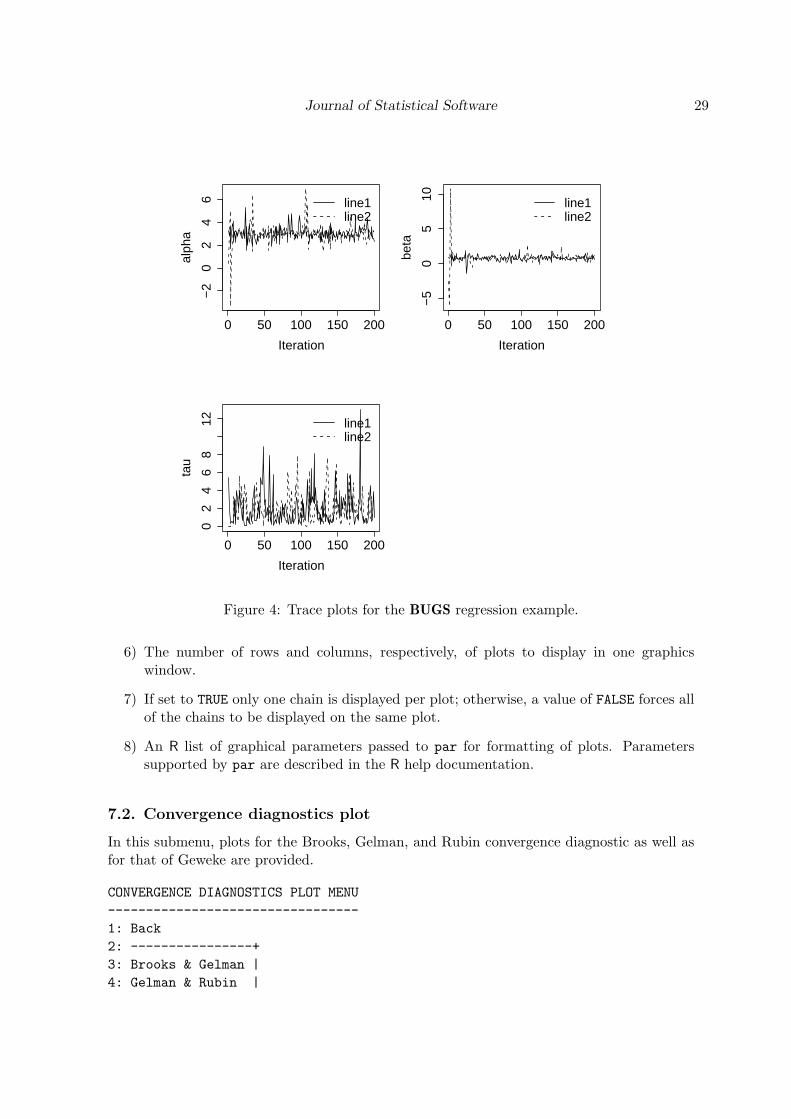
Trace
Trace plots show a time series plot of the individual, sampled value for each parameter ineach chain, as shown in Figure 4.
Journal of Statistical Software 27
−4 −2 0 2 4 6 8
0.0
0.4
0.8
alpha
Den
sity
line1line2
−5 0 5 10
0.0
0.5
1.0
1.5
beta
Den
sity
line1line2
0 5 10
0.0
0.2
0.4
tau
Den
sity
line1line2
Figure 2: Posterior marginal distributions for the BUGS regression example.
Options. . .
This submenu allows users to change the previously described settings for the descriptiveplots.
Specify parameter to change or press <ENTER> to continue
The options appearing in the “Graphics” category control the general layout of plots. Briefdescriptions are as follows:
3) If set to TRUE legends are included in the plots; otherwise, a value of FALSE will suppressplot legends.
4) If set to TRUE titles are added to the plots; otherwise, a value of FALSE will suppressplot titles.
5) If set to TRUE all plots generated in BOA will be kept open; otherwise, a value of FALSEindicates that only the most recently opened plots be kept open.
Journal of Statistical Software 29
0 50 100 150 200
−2
02
46
Iteration
alph
a
line1line2
0 50 100 150 200
−5
05
10
Iteration
beta
line1line2
0 50 100 150 200
02
46
812
Iteration
tau
line1line2
Figure 4: Trace plots for the BUGS regression example.
6) The number of rows and columns, respectively, of plots to display in one graphicswindow.
7) If set to TRUE only one chain is displayed per plot; otherwise, a value of FALSE forces allof the chains to be displayed on the same plot.
8) An R list of graphical parameters passed to par for formatting of plots. Parameterssupported by par are described in the R help documentation.
7.2. Convergence diagnostics plot
In this submenu, plots for the Brooks, Gelman, and Rubin convergence diagnostic as well asfor that of Geweke are provided.
30 boa: MCMC Output Convergence Assessment and Posterior Inference in R
5: Geweke |6: Options... |7: ----------------+
Brooks and Gelman
Included in the Brooks and Gelman plot are the multivariate potential scale reduction factorand the maximum of the potential scale reduction factors (see Section 6.2.1) for successivelylarger segments of the chains. The first segment contains the first 50 iterations. The remainingiterations are then partitioned into equal bins and added incrementally to construct theremaining segments. Option 1 of Section 7.2.4 controls the number of bins used for theplot. Scale factors are plotted against the maximum iteration number in the segments. Cubicsplines are used to interpolate through the point estimates for the segments.
Gelman and Rubin
Gelman and Rubin plots display the corrected potential scale reduction factors (see Section6.2.1) for each parameter in successively larger segments of the chain. The first segmentcontains the first 50 iterations. The remaining iterations are then partitioned into equal binsand added incrementally to construct the remaining segments. Options 5 and 6 of Section 7.2.4control the error rate for the upper quantile and the number of bins, respectively. Option7 determines the proportion of samples, from the end of the chains, to be included in theanalysis. The scale factor is plotted against the maximum iteration number for the segment.Cubic splines are used to interpolate through the point estimates for the segments.
50 100 150 200
1.00
1.05
1.10
1.15
1.20
1.25
Last Iteration in Segment
Shr
ink
Fac
tor
RpRmax
Figure 5: Brooks and Gelman diagnostic plot for the BUGS regression example.
Journal of Statistical Software 31
50 100 150 200
1.0
1.4
1.8
alpha
Last Iteration in Segment
Shr
ink
Fac
tor 97.5%
Median
50 100 150 200
1.0
1.2
1.4
1.6
beta
Last Iteration in Segment
Shr
ink
Fac
tor 97.5%
Median
50 100 150 200
1.0
1.4
1.8
2.2
tau
Last Iteration in Segment
Shr
ink
Fac
tor 97.5%
Median
Figure 6: Gelman and Rubin diagnostic plots for the BUGS regression example.
Geweke
Geweke plots include the Z statistic values (see Section 6.2.2) for each parameter in suc-cessively smaller segments of the chain. Each k = 1, . . . ,K segment contains the last(K − k + 1)/K × 100% of the iterations in the chain. Options 8 and 9 of Section 7.2.4set the error rate for the confidence bounds and the number of bins included in the plot,respectively. Options 10 and 11 control the fraction of iterations covered by the windowsfor the Geweke diagnostic calculation. In certain instances, smaller subsets may contain toofew iterations to evaluate the test statistic. Such segments, if they exist, are automaticallyomitted from the plot. The test statistic is plotted against the minimum iteration number forthe segment.
Options. . .
This submenu allows users to change the previously described settings for the plotting ofconvergence diagnostics.
The Window menu allows users to switch between and save the active graphics windows.
WINDOW 2 MENU=============1: Back2: ------------------------+3: Previous |4: Next |5: Save to Postscript File |6: Close |7: Close All |8: ------------------------+
The number of the active graphics window is displayed in the title of this menu. In this case,the active window is graphics window 2.
34 boa: MCMC Output Convergence Assessment and Posterior Inference in R
9.1. Previous
Makes the previous graphics window in the list of open windows the active graphics window.
9.2. Next
Makes the next graphics window in the list of open windows the active graphics window.
9.3. Save to postscript file
Saves the active graphics window to a postscript file. The user is prompted to enter the nameof the postscript file in which to save the graphics window.
Enter name of file to which to save the plot [none]
The name of the file should be given, without the directory path. The file will automaticallybe saved in the Working Directory (see Section 4.1.5). Microsoft Windows users can save thegraphics window in other formats directly from the R program menus.
9.4. Close
Closes the active graphics window.
9.5. Close all
Closes all graphics windows that were opened during the current boa session.
References
Applegate D, Kannan R, Polson NG (1990). “Random Polynomial Time Algorithms forSampling from Joint Distributions.” Technical Report 500, Carnegie-Mellon University.
Best N, Cowles MK, Vines K (1995). CODA: Convergence Diagnosis and Output AnalysisSoftware for Gibbs Sampling Output, Version 0.30. MRC Biostatistics Unit, University ofCambridge, Cambridge, UK. URL http://citeseer.ist.psu.edu/best97coda.html.
Brooks S, Gelman A (1998). “General Methods for Monitoring Convergence of IterativeSimulations.” Journal of Computational and Graphical Statistics, 7(4), 434–455.
Brooks SP, Roberts GO (1998). “Convergence Assessment Techniques for Markov ChainMonte Carlo.” Statistics and Computing, 8(4), 319–335.
Cowles MK, Carlin BP (1996). “Markov Chain Monte Carlo Convergence Diagnostics: AComparative Review.” Journal of the American Statistical Association, 91, 883–904.
Gelman A, Rubin DB (1992). “Inference from Iterative Simulation Using Multiple Sequences.”Statistical Science, 7, 457–511.
Geweke J (1992). Bayesian Statistics, volume 4, chapter Evaluating the Accuracy of Sampling-Based Approaches to Calculating Posterior Moments. Oxford University Press, New York.
Gilks WR, Wild P (1992). “Adaptive Rejection Sampling for Gibbs Sampling.” AppliedStatistics, 41(2), 337–348.
Hastings WK (1970). “Monte Carlo Sampling Methods Using Markov Chains and their Ap-plications.” Biometrika, 57, 97–109.
Heidelberger P, Welch P (1983). “Simulation Run Length Control in the Presence of an InitialTransient.” Operations Research, 31, 1109–1144.
Jennison C (1993). “Discussion of “Bayesian Computation via the Gibbs Sampler and RelatedMarkov Chain Monte Carlo Methods”.” Journal of the Royal Statistical Society B, 55, 54–56.
Neal RM (2003). “Slice Sampling.” Annals of Statistics, 31, 705–767.
Plummer M, Best N, Cowles K, Vines K (2006). “coda: Convergence Diagnosis and Out-put Analysis for MCMC.” R News, 6(1), 7–11. URL http://CRAN.R-project.org/doc/Rnews/.
Raftery AL, Lewis S (1992). Bayesian Statistics, volume 4, chapter How Many Iterations inthe Gibbs Sampler? Oxford University Press, New York.
R Development Core Team (2006). R: A Language and Environment for Statistical Computing.R Foundation for Statistical Computing, Vienna, Austria. ISBN 3-900051-07-0, URL http://www.R-project.org/.
Schruben LW, Signh H, Tierney L (1983). “Optimal Tests for Initialization Bias in SimulationOutput.” Operations Research, 31, 1167–1178.
Spiegelhalter D, Thomas A, Best N, Gilks W (1996). BUGS 0.5 Bayesian Inference UsingGibbs Sampling Manual. MRC Biostatistics Unit, Institute of Public Health, Cambridge,UK, version ii edition.
Thomas A, Best N, Spiegelhalter D (2000). “WinBUGS – A Bayesian Modelling Framework:Concepts, Structure, and Extensibility.” Statistics and Computing, 10(4), 325–337.
Thomas A, O’Hara B, Ligges U, Sturtz S (2006). “Making BUGS Open.” R News, 6(1),12–17. URL http://CRAN.R-project.org/doc/Rnews/.
36 boa: MCMC Output Convergence Assessment and Posterior Inference in R
A. R programming
A.1. Format of R output
The options function in R can be used to control the format of outputted text in boa. Thiscan be done prior to starting the boa menu. To set the number of significant digits to bedisplayed, type
R> options(digits = <value>)
where <value> is the desired number of significant digits. The number of characters allowedper line can be controlled with the command
R> options(width = <value>)
where <value> is the desired number of characters to display per line.
A.2. Syntax for R vectors
Several menu items in boa allow users to input vectors of data. Vectors in R can be suppliedin a number of ways. The simplest is with the concatenation function c:
R> c(<element 1>, <element 2>, ..., <element n>)
where the elements may be numbers, logical values, or character strings. Another way toconstruct vectors is with the seq function:
R> seq(<starting value>, <ending value>, length = <number of values>)
or
R> seq(<starting value>, <ending value>, by = <step size>)
where length defines the number of values in the vector and by defines the spacing betweensuccessive values in the vector. The : operator, which is a special case of the seq function,can also be used to construct vectors. This operator is used as follows:
R> <starting value>:<ending value>
which is equivalent to the command seq(<starting value>, <ending value>, by = 1).More detailed descriptions of these functions can be found in the R help documentation.
Journal of Statistical Software 37
Affiliation:
Brian J. SmithDepartment of BiostatisticsThe University of Iowa200 Hawkins Drive, C22 GHIowa City, IA 52242-1009, United States of AmericaE-mail: [email protected]: http://www.public-health.uiowa.edu/academics/faculty/brian_smith.html
Journal of Statistical Software http://www.jstatsoft.org/published by the American Statistical Association http://www.amstat.org/