Board of the Foundation of the Scandinavian Journal of ...abe/lista/pdf4R8xPVzCnX.pdf · Board of...

Board of the Foundation of the Scandinavian Journal of Statistics

A Simple Sequentially Rejective Multiple Test ProcedureAuthor(s): Sture HolmSource: Scandinavian Journal of Statistics, Vol. 6, No. 2 (1979), pp. 65-70Published by: Wiley on behalf of Board of the Foundation of the Scandinavian Journal of StatisticsStable URL: http://www.jstor.org/stable/4615733 .

Accessed: 09/10/2013 08:15

Your use of the JSTOR archive indicates your acceptance of the Terms & Conditions of Use, available at .http://www.jstor.org/page/info/about/policies/terms.jsp

.JSTOR is a not-for-profit service that helps scholars, researchers, and students discover, use, and build upon a wide range ofcontent in a trusted digital archive. We use information technology and tools to increase productivity and facilitate new formsof scholarship. For more information about JSTOR, please contact [email protected].

.

Wiley and Board of the Foundation of the Scandinavian Journal of Statistics are collaborating with JSTOR todigitize, preserve and extend access to Scandinavian Journal of Statistics.

http://www.jstor.org

This content downloaded from 143.107.183.117 on Wed, 9 Oct 2013 08:15:53 AMAll use subject to JSTOR Terms and Conditions

http://www.jstor.org/action/showPublisher?publisherCode=black

http://www.jstor.org/action/showPublisher?publisherCode=bfsjs

http://www.jstor.org/stable/4615733?origin=JSTOR-pdf

http://www.jstor.org/page/info/about/policies/terms.jsp


Scand J Statist 6: 65-70, 1979

A Simple Sequentially Rejective Multiple Test Procedure

STURE HOLM

Chalmers University of Technology, Goteborg

Received December 1977, revised September 1978

ABSTRACT. This paper presents a simple and widely ap- plicable multiple test procedure of the sequentially rejective type, i.e. hypotheses are rejected one at a tine until no further rejections can be done. It is shown that the test has a prescribed level of significance protection against error of the first kind for any combination of true hypotheses. The power properties of the test and a number of possible applications are also discussed.

Key words: multiple test, simultaneous test

1. Introduction

The statistical problems arising in applications often involve a number of detail problems, i.e. there are often a number of interesting parameters to be esti- mated and/or a number of interesting hypotheses to be tested. In some cases these detail problems may be treated separately without any connection to each other. But in most cases the detail problems are connected to each other and the totality of solutions to the detail problems are used to get a general picture. In this latter case the statistician is faced with a multiple statistical inference problem, where he has to take into consideration that the different detail problems should be treated simultaneously.

Multiple statistical inference has been a vital research area within statistical inference theory the past 50 years, and methods have been proposed for several situations of practical interest. A good presentation of the earlier main results is given by Miller (1966). The multiple statistical inference methods are separated into two main types, multiple confidence interval methods and multiple test methods.

For multiple test procedures there has been suggested several types of properties, which the tests should have in order to give satisfactory protection against wrong decisions. Some of those are based on decision theoretic conceptions, while others are based on probabilities of making wrong decisions. In this paper we will study multiple test procedures and we will use the most common type of protection against error of the first kind by requiring the tests to have a small probability of rejecting any true hypotheses.

The methodological motivation and exact definition is the following.

Let the (detail) hypotheses in a multiple test problem be denoted by H1, H12, ..., Hn and the alternatives to those by K., K2, ..., K,. A (non-randomized) multiple test procedure is a rule assigning to each outcome a set of rejected hypotheses (which might be empty). This means that there are also n critical regions C1, C2, ..., Cn consisting of those outcomes for which the corresponding hypotheses are rejected.

In a test of a single null hypothesis H1 against an alternative K1 the size of the test is defined as the supremum of the probability of the critical region C1 when the hypothesis H11 is true. This probability of error of the first kind is always kept at (or below) a small predetermined level a. The philosophical reason for this is that when we have made a 'discovery' by rejecting the null hypothesis we can quite safely claim that the null hypothesis is not true, because if it was true, we should have accepted it with a probability of at least 1 -oc. This also implies that we do not make any 'discovery' by accepting the null hypotheses, because we do not have such a protection against errors of the second kind.

In a multiple test of a number of hypotheses H,, H12, ..., Hn there are a lot of possible combinations of null hypotheses. If we want to make our 'discoveries' in form of rejected null hypotheses to be safely claimed, we must keep the probability of rejecting any true null hypotheses small, how many and which the true hypotheses may be. Thus we are led to the following definition

Definition. A multiple test procedure with critical regions C1, C2, ..., Cn for testing hypotheses Hi, H2, ..., H,, is said to have a multiple level of significance a (for free combinations) if for any non-empty index set I' {1, 2, 3, ..., n} the supremum of the probability P( u iE C2) when Hi are true for all i eI is smaller than or equal to a.

The words 'for free combinations' are put into the definition in order to underline that all subsets of

5 - 791923 Scand J Statist 6



66 S. Holm

null hypotheses could appear as the set of true hypotheses. There might be situations in which all subsets are not allowed for some reason, for instance situations where the truth of two hypotheses implies the truth or falseness of a third hypothesis. It is to be observed that a multiple level of significance ac for some restricted combinations imposes fewer conditions on the test procedure than a multiple level of significance a for free combinations, i.e. a test procedure with multiple level of significance x for free combinations has a multiple level of significance a for any type of restricted combinations.

In our setting the basic hypotheses H1, H2, ..., H. are minimal in the sense of Gabriel (1969). This means that if o,, con, ..., on are the parameter sets where the hypotheses H1, H2, ..., Hn are true than the only (secondary) hypotheses to be tested are the hypotheses that the parameter belongs to intersections nf EI co, of sets coi for different index sets Ic- {1, 2, ..., n}.

We will exclusively discuss a type of multiple test procedures, which may be called sequentially rejective because basic hypotheses are rejected one at a time according to certain rules. Thus we do not make separate tests of all the (secondary) hypotheses that the parameter belongs to intersections nflI wi for different Ic {1, 2, ..., n}. We always consider such (secondary) hypotheses to be rejected as soon as any of the included basic hypotheses are rejected.

A test procedure is called coherent if it prevents the contradiction of rejecting a hypothesis without also rejecting all other hypotheses implying it. It is called consonant if it avoids dissonances consisting in rejecting a hypothesis and not rejecting any other hypotheses implied by it. (See Gabriel, 1969, pp. 229 and 231.) The sequentially rejective tests are coherent and consonant by their very definition.

In many applications there are logical implications among the basic hypotheses i.e. some combinations of falseness of different basic hypotheses are not allowed because there are no possible parameter points corresponding to those combinations. Then we do not want the multiple test procedure to end up with a statement that the parameter belongs to such an empty set. This requirement has to be studied separately for each kind of logical implication. We will consider only the type of logical implications arising when we have two-sided alternatives for some parameters, and want to make one- sided statements.

The sequentially rejective multiple tests are not completely new. Tests of the same type are discussed by Naik (1975, p. 522), and the consonant closed procedures discussed by Marcus et al. (1976, p. 656) are equivalent to sequentially rejective tests. Marcus et al. (1976) give one particular example of such a

test in an analysis of variance situation, and indicate that others can be constructed. But they do not seem to have thought of the simple and general procedure we present in the next section, because that procedure can easily be used to make one-sided rejections, which they have posed as a difficult problem. Our test is based on the simple Boole inequality and can be applied to any parametric or non-parametric model, but yet it has good power properties. It will be shown by examples that it may have considerably higher power than classical multiple test procedures. It also has surprisingly small loss of power compared to the special sequentially rejective tests (or equivalent consonant closed tests) that can be constructed in different parametric models, for instance analysis of variance models.

2. A simple sequentially rejective test

In this section we will present a simple sequentially rejective test, which is based on the Boole inequality. The use of the Boole inequality within multiple inference theory is usually called the Bonferroni technique, and for this reason we will call our test the sequentially rejective Bonferroni test.

When the n hypotheses H,, H2, ..., Hn are tested separately by using tests with the level ac/n it follows immediately from the Boole inequality that the probability of rejecting any true hypotheses is smaller then or equal to ac. This constitutes then a multiple test procedure with the multiple level of significance a for free combination, the classical Bonferroni multiple test procedure.

The separate tests in the classical Bonferroni multiple test are usually performed by using some test statistics, which we will denote here by Y,, Y2, ..., Yn. We suppose now that this is the case, and also that these test statistics have a tendency of obtaining greater values when the corresponding hypothesis is not true. The critical level Sk(Y) for the outcome y of the test statistic Yk is then equal to the supremum of the probability P(Yk >y) when the hypothesis Hk is true. Defining now the obtained levels Rl, R2, ..., Rn by

Rk = dk(Yk)

the classical Bonferroni test can be performed by comparing all the obtained levels R&, R2, ..., Rn with a/n.

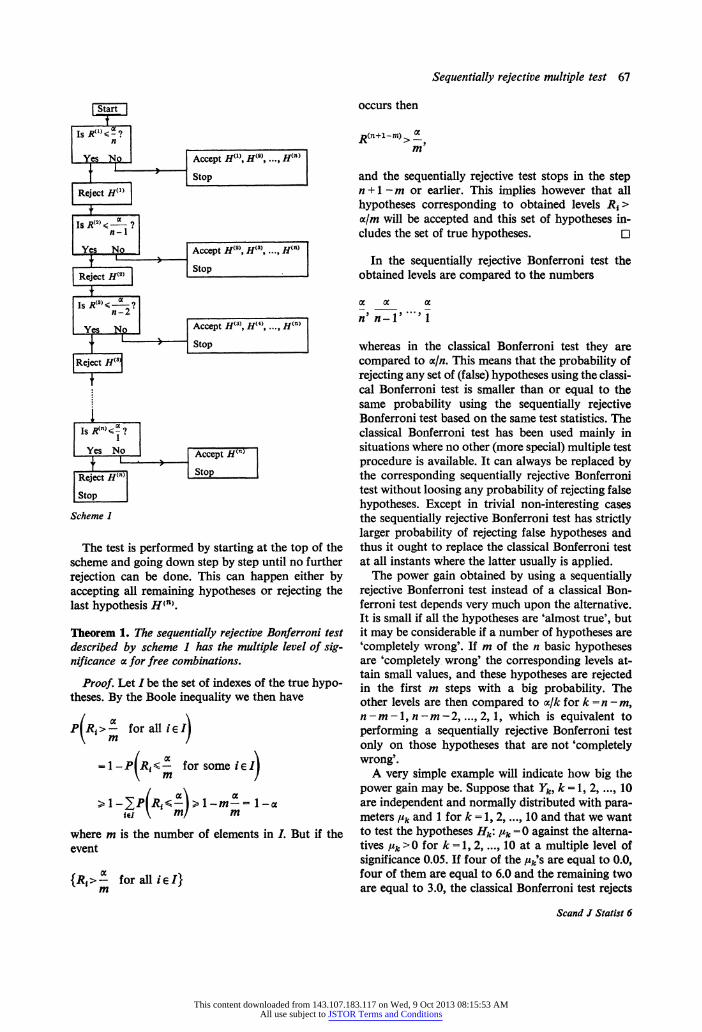
The sequentially rejective Bonferroni test will also be defined by the obtained levels. Denoting by R('1 < R'2' 6 ... <R(n, the ordered obtained levels and by H"), H , ..., H'() the corresponding hypotheses, the procedure can most easily be described by scheme 1, where ac, 0 <La < 1, is a fixed number.

Scand J Statist 6



Start

Is R(1 <-? n

Yes No Accept H(l) H(2), Hn

Stop

Reject H()1

I (2) <; a ; IsR - n-l

Yes No Accept 2 H

Reject H(2) Stop

Is R(3) < ? n-2

es Accept H(3), H(), H(.).

i t

Stop

Reject H'9

Is Rkn) <? -

Yes No Accept H(n)

Reject H(n| Stop

Stop

Scheme I

The test is performed by starting at the top of the scheme and going down step by step until no further rejection can be done. This can happen either by accepting all remaining hypotheses or rejecting the last hypothesis H(n).

Theorem 1. The sequentially rejective Bonferroni test described by scheme I has the multiple level of significance a for free combinations.

Proof. Let I be the set of indexes of the true hypotheses. By the Boole inequality we then have

P Rf >- for all i e m

=1-P(R<- for some iEl)

where m is the number of elements in I. But if the event

{Ri >- for all i e I} m

occurs then

.R(n + i-M)> ?:,. m

and the sequentially rejective test stops in the step n +1 - m or earlier. This implies however that all hypotheses corresponding to obtained levels Ri > ac/m will be accepted and this set of hypotheses in- cludes the set of true hypotheses. O

In the sequentially rejective Bonferroni test the obtained levels are compared to the numbers

ac ac ac n' n-I' '

whereas in the classical Bonferroni test they are compared to a/n. This means that the probability of rejecting any set of (false) hypotheses using the classical Bonferroni test is smaller than or equal to the same probability using the sequentially rejective Bonferroni test based on the same test statistics. The classical Bonferroni test has been used mainly in situations where no other (more special) multiple test procedure is available. It can always be replaced by the corresponding sequentially rejective Bonferroni test without loosing any probability of rejecting false hypotheses. Except in trivial non-interesting cases the sequentially rejective Bonferroni test has strictly larger probability of rejecting false hypotheses and thus it ought to replace the classical Bonferroni test at all instants where the latter usually is applied.

The power gain obtained by using a sequentially rejective Bonferroni test instead of a classical Bon- ferroni test depends very much upon the alternative. It is small if all the hypotheses are 'almost true', but it may be considerable if a number of hypotheses are 'completely wrong'. If m of the n basic hypotheses are 'completely wrong' the corresponding levels at- tain small values, and these hypotheses are rejected in the first m steps with a big probability. The other levels are then compared to ac/k for k = n -m, n-rm-l, n-rm -2, ..., 2, 1, which is equivalent to performing a sequentially rejective Bonferroni test only on those hypotheses that are not 'completely wrong'.

A very simple example will indicate how big the power gain may be. Suppose that Yk, k = 1, 2, ..., 10 are independent and normally distributed with parameters Ilk and 1 for k = 1, 2, ..., 10 and that we want to test the hypotheses Hk: k = 0 against the alternatives Ilk >0 for k = 1, 2, ..., 10 at a multiple level of significance 0.05. If four of the Puk's are equal to 0.0, four of them are equal to 6.0 and the remaining two are equal to 3.0, the classical Bonferroni test rejects

Sequentially rejective multiple test 67

Scand J Statist 6



68 S. Holm

both the latter hypotheses with probability 0.439, while the sequentially rejective Bonferroni procedure rejects both with probability 0.565.

The great advantage with the sequentially rejective Bonferroni test (as well as with the classical Bon- ferroni test) is its flexibility. There are no restrictions on the type of tests, the only requirement being that it should be possible to calculate the obtained level for each separate test. Further there are no problems in including in the analysis only the a priori interesting hypotheses, while more special multiple tests usually include all hypotheses of a certain kind. But when there exist logical implications among the hypotheses problems arise which we have to take in- to consideration.

Let as before wl, w02, Ct3, ..., on denote the parameter sets where the hypotheses H1, H2, H3, ..., Hn are true. Then there exists a logical implication as soon as there is some index set Isuch that nieiC Oi = b. In words this means that some combination of

falseness of the different hypotheses is not possible, and the natural condition is of course that we should not end up the multiple test with a statement that the true parameter point is in an empty set. Each type of logical implication requires a special analysis of the properties of the test statistics in order to ensure that the test can not end up with such statements. The only type of logical implication we will consider is the one arising in connection with two-sided rejections.

Let y be a (one-dimensional) parameter and suppose that H1: y < yO and H2: y > y2o are basic hypotheses in a multiple test problem. Then C a,l n C co2 = b and both these hypotheses should not be rejected

in the multiple test procedure. It is natural to use the same test statistic to test both hypotheses and since we have the convention of rejecting the hypotheses for high values of the test statistics we should have Y2= - Y1. Now for the outcomes Yi of Y1 and y= -Yl for Y2 the obtained levels ail(yi) and A2(Y2) satisfy

Y2)UP P(Y2 > Y2) V>Yo

> sup P(Y2 > Y2) = sup (1 -P(Y2 < Y2)) V=YO Y=Yo

= sup (1 - P(Y1 > y1)) Y=Yo

= 1 - inf P(Y1 < y1) Y='Yo

> 1 - inf P(Y1 > y1) Y=VYo

> 1 -sup P(Y1 > y1) V=Yo

> 1-sup P(Y1 > Ay1)1 l(y) V?Yo

This means that for any outcomes Yi and Y2 ̀ Y1 of Y1 and Y2 at least one of the obtained levels Mi(Y,) and d2(Y2) is >, and thus both hypotheses H1 and H2 can not be rejected in a sequentially rejective Bonferroni test (or a classical Bonferroni test) for any multiple level of significance cx 6 i.

If there are a number of pairs of one-sided hypotheses and no logical implications beside those within the pairs all illogical statements will still be avoided if the same statistics with opposite signs are used within the pairs and the multiple level of significance oc is smaller than or equal to 1. These tests are also coherent and consonant.

3. Applications and extensions

The sequentially rejective Bonferroni test can be applied in all situations where the classical Bonferroni test is usually applied. And it ought to replace the classical Bonferroni test in these cases because it gives only slightly more complicated computations and a non-negligable increase of power. It should however be noted that the sequentially rejective Bon- ferroni test can not be used to construct smaller confidence sets than those constructed by the classical Bonferroni test. This is so because the confidence set consists of the parameter points that would not be rejected as true parameter points in separate single tests. And when a confidence set is constructed from multiple tests it consists of the parameter points for which none of the detail hypotheses are rejected, which is in fact a special construction of a single test from a multiple test. If the sequentially rejective Bon- ferroni test is used in this way it is equivalent to the classical Bonferroni test.

The great advantage of the sequentially rejective Bonferroni test (as well as the classical Bonferroni test) is its computational simplicity, which arises from the reduction of the distributional problems to one dimension when the Boole inequality is used. The same computational simplicity is obtained when the test statistics are independent. It is easily seen that a sequentially rejective procedure with multiple level of significance a can be constructed by replacing the comparison constants c/n, cx/(n -1), ..., c/1 in the sequentially rejective Bonferroni test by 1 - (1 - c)11', 1 - (1 - c)1/(nl1)' ..., 1 - (1 - cc)1, which are greater. This means that we get a more powerful test, but the increase in power is not very big. Among the numerous possible applications of the sequentially rejective Bonferroni test we will next mention a few.

The problem of comparing several treatments with one control have been studied by several authors. For the case of normally distributed observations the multiple test procedure suggested by Dunnett (1955) is commonly used. It requires the same number of

Scand J Statist 6



Sequentially rejective multiple test 69

observations for all treatments, and it is based on the assumption that the variance is the same for the control and all treatments. Marcus et al. (1976) have proposed a closed test procedure, which is a refine- ment of the Dunnett procedure and which is more powerful. Their procedure is equivalent to a sequentially rejective procedure presented in Holm (1977).

The sequentially rejective Bonferroni test can also be used in this situation although it is of course less powerful than the refined Dunnett test. In most cases the difference is however not very big. In order to illustrate this we consider the case of comparing 9 treatments with one control based on four observations for the control and for each treatment. The refined Dunnett test then consists in successively comparing the ordered individual t-statistics for comparing one treatment with the control with the numbers

1.70, 1.99, 2.15, 2.25, 2.33, 2.40, 2.45, 2.50, 2.54,

while the sequentially rejective Bonferroni test consists in successively comparing the same statistics with the numbers

1.70, 2.04, 2.23, 2.36, 2.46, 2.54, 2.60, 2.66, 2.71.

In the classical Dunnett test they are all compared to 2.54.

There are two different variations of this problem, where the sequentially rejective Bonferroni test can easily be applied, whereas the classical and the refined Dunnett test can not so easily be applied. One is the case of non-equal sample sizes. Then the classical Dunnett type of test requires much computation, because tables are not available. The corresponding closed procedure requires even more computation, since a number of critical values of classical Dunnett test statistics are needed. The sequentially rejective Bonferroni test requires only a number of critical values of ordinary t statistics.

The other variation is the case where one-sided rejections are wanted. This is easily obtained by using a sequentially rejective Bonferroni test and introducing two one-sided hypotheses for each comparison of a treatment with the control.

For comparison of a number of treatments with one control in the case of non-normal distribution a many-one-rank test can be used. Such a test can be refined to a corresponding sequentially rejective test (equivalent to a corresponding closed test) with a higher power. See Holm (1977). If the number of observations are not the same for all treatments and the control, computational problems arise since tables are not available. These difficulties are avoided if a sequentially rejective Bonferroni test is used, since a table for the ordinary two-sample Wilcoxon test statistic is the only table needed for this test.

In the analysis of contingency tables the distributional problems connected with the construction of simultaneous tests are so big that the only possibility in practice is to use the Bonferroni technique. See e.g. Haberman (1974) chapter four. In such cases the power would be higher if the sequentially rejective Bonferroni test was used instead of a classical Bon- ferroni test. Other fields where big computational problems call for the use of Bonferroni technique are time series analysis and analysis of multidimensional distributions.

In all these cases as well as in others it may happen that some hypotheses are more important than the others, which may imply the use of higher levels of significance for the most important hypotheses and smaller levels of significance for the less important hypotheses when the Bonferroni technique is applied. At a first glance it seems to be impossible to obtain such an arrangement with the sequentially rejective Bonferroni test. But this is not true, since it is possible to generalise Theorem 1 to the case of different weights by slightly changing the procedure.

Let as before H1, H2, ..., Hn, be the hypotheses to be tested and R1, R2, ..., Rn be the obtained levels of some suitable test statistics for those hypotheses. Further let cl, c2, ..., cn be positive constants in- dicating the importance of the hypotheses in the sense that the constants corresponding to more important hypotheses are greater then those corresponding to less important hypotheses. The precise meaning of these constants will be made clear later. Now introduce the statistics Sk = Rklck for k = 1, 2, n, let S S') 1SS21 < ... <S(') be the ordered statistics in this series, let H(l), H', ..., H'n) be the corresponding hypotheses and let C c'2, ..., c (n) be the corresponding constants. Then a generalized sequentially rejective Bonferroni test can be described by scheme 2 on the next page.

Theorem 2. The generalized sequentially rejective Bon- ferroni test described by scheme 2 has the multiple level of significance oc for free combinations.

Proof. Let I be the set of indexes for the true hypotheses. By the Boole inequality we have

P(Si >- M

for all i e I) JCI

= 1 - P(Si < E for some i E I)

j6I

ciac =1-P(RA i for some iEI)

jeI

ci-c >l_2Ei

= 1-a.

{eI *~c jeI

Scand J Statist 6



70 S. Holm

Is s n Ec(k)

k=l Accept H('), H(2), H (n)

Yes No

t ' I Stop

Reject H"'

.

Is ,,(2) a E c (k)@

k-2 Accept Hf'), Hff H)(n)

Yes No f I ~~~~~Stop

Reject H(2)

Is . S(3) < a ? E c(k)

k=3 N Accept H'3', H(4) H(n)-

s , ' y ~~~Stop

Reject 11"

Yes No Accept l

t I

> LStop Reject H"3 Stop

Scheme 2

Now suppose that the event

St > - for all i e I}

JEI

occurs, and let v be the smallest order number in the series S(1)< (2)<... <S (n) attained by the variables {St: iE I}. Then

S(y) > - -x c

fI na c(l J=v

which implies that the procedure will stop in step v or earlier and that all true hypotheses will be accepted. E

From the definition of the generalized sequentially rejective Bonferroni test and the proof of Theorem 2 it can easily be seen what role is played by the constants cl, c2, ..., cn. At each step in the procedure the obtained levels for the not yet rejected hypotheses

are compared to parts of a, which are proportional to the corresponding constants. Compared to the 'ordinary' sequentially rejective Bonferroni test this implies an increase of power for alternative to hypotheses with high values of ck at the cost of decrease of power for alternatives to hypotheses with small values of Ck, which is the reason of introducing the generalized test. When all Ck are equal the generalized test reduces to the ordinary test.

The previous discussion indicates a good way of handling multiple test problems in complicated applications. One can start by choosing a number of relevant hypotheses, then assign to every hypothesis a suitable test statistic, whose one-dimensional distribution is known exactly or approximately, and finally direct the power towards the most important hypotheses by choosing proper constants in a generalized sequentially rejective Bonferroni test. Of course it is also a desire to have the different test statistics exactly or approximately independent not for computational reasons but because a good experimental design requires the different hypotheses to be tested by variables 'not related to each others'.

Acknowledgement

The referee's suggestions for improving the presentation are gratefully acknowledged.

References

Dunnett, C. W. (1955). A multiple comparison procedure for comparing several treatments with a control. J. Amer. Statist. Assoc. 50, 1096-1121.

Gabriel, K. R. (1969). Simultaneous test procedures-some theory of multiple comparisons. Ann. Math. Statist. 40, 224-250.

Haberman, S. J. (1974). The analysis of frequency data. The University of Chicago Press.

Holm, S. A. (1977). Sequentially rejective multiple test procedures. Statistical research report 1977-1, University of UmeA, Sweden.

Marcus, R., Peritz, E. & Gabriel, K. R. (1976). On closed testing procedures with special reference to ordered analysis of variance. Biometrika 63, 655-660.

Miller, R. G., Jr. (1966). Simultaneous statistical inference. McGraw-Hill, New York.

Naik, U. D. (1975). Some selection rules for comparing p processes with a standard. Communications in Statistics 4, 519-535.

Sture Holm Department of Mathematics Chalmers University of Technology S-412 96 Goteborg Sweden

Scand J Statist 6



Date post:	11-Nov-2018
Category:	Documents
Upload:	phamthu
View:	214 times
Download:	0 times

Board of the Foundation of the Scandinavian Journal of ...abe/lista/pdf4R8xPVzCnX.pdf · Board of...

Documents