Bond Graph Model Based on Structural Diagnosability and Recoverability Analysis: Application to...

986 IEEE TRANSACTIONS ON VEHICULAR TECHNOLOGY, VOL. 61, NO. 3, MARCH 2012

Bond Graph Model Based on StructuralDiagnosability and Recoverability Analysis:

Application to Intelligent Autonomous VehiclesRui Loureiro, Rochdi Merzouki, and Belkacem Ould Bouamama

Abstract—A controlled system can be subjected to faults, whichmay cause unexpected system dynamics that prevent the systemobjectives to be achieved. This paper introduces the problem ofstructural fault-tolerance analysis of actuator, sensor, and plantfaults with respect to diagnosability and recoverability conditions.Existing methods in the literature usually investigate the faulttolerance of systems separately from fault diagnosis, even if theyare strongly related. The bond graph (BG) tool is an adequate toolfor dynamic modeling of complex systems and performing faultdetection and isolation. The innovative interest of the proposedapproach is to extend the use of this tool for verification ofstructural recoverability conditions by exploiting the behavioral,structural, and causal properties of the BG tool. The obtainedstructural technique is then applied to an intelligent autonomousvehicle named RobuCar with decentralized inputs and outputs.

Index Terms—Fault diagnosis, fault tolerance, intelligent sys-tems, modeling.

I. INTRODUCTION

P ROCESS systems safety has become an important issue inthe field of automatic control systems. These types of sys-

tems often work at a high level of performance, which may leadto the occurrence of equipment faults. To avoid faults provokinga system shut down, or even accidents, the concept of fault-tolerant systems (FTs) has been introduced in process systemssuch as nuclear power plants and aircraft. Fault detection andisolation (FDI) and fault-tolerant control (FTC) problems arethe main issues when dealing with FTs. They are essentiallybased on redundancy analysis. Redundancy is available in asystem when a task can be performed by alternative means,and it can be made available in the form of material and/oranalytical redundancy. As referred in [1], the former existswhen identical hardware/software components are arranged inparallel, and it can be presented in the form of duplex ortriplex redundancy, etc. Analytical redundancy has to do withthe ability to use static/dynamic relations between variables

Manuscript received July 30, 2011; revised December 1, 2011; acceptedJanuary 22, 2012. Date of publication February 3, 2012; date of current versionMarch 21, 2012. This work was supported by European funds in the frameworkof the Intelligent Transport for Dynamic Environment Project 019C from theInterreg IVB NWE Program. The review of this paper was coordinated byProf. F. Assadian.

The authors are with Ecole Polytechnique Universitaire de Lille, 59000Villeneuve d ’Ascq, Lille, France (e-mail: [email protected];[email protected]; [email protected]).

Color versions of one or more of the figures in this paper are available onlineat http://ieeexplore.ieee.org.

Digital Object Identifier 10.1109/TVT.2012.2186472

associated with the system components. In [2], FTC strategieswere divided into passive and active approaches. In this paper,only the active approaches were considered. The latter makeuse of the fault information provided by FDI algorithms tomodify the control system so that the FT’s objectives remainachievable, even with less performance. In the work presentedin [3], a bibliographical review of several works on active FTC(AFTC) strategies was presented.

Although the ability to isolate a fault and perform AFTCstrategies is strongly related, most of consulted papers devotedto study the level of system FT [1], [4]–[7] assume that theFDI step is performed, instead of also basing their analysison the diagnosis capabilities of the system. These works useanalytical models under state space format. Moreover, its mainidea is to verify system input or output redundancy and if therequired energy to perform reconfiguration strategies is accept-able. However, in the referred works, only actuator and sensorfaults are considered. In addition, the mathematical model ofthe system is supposed to be under a linear or a class of nonlin-ear system format. Furthermore, analytical approaches requireaccurate models and numerical values of the parameters, whichare not always available in real systems. This is why graphicalapproaches based on the system model can be an alternative tostudy fault diagnosability and fault recoverability possibilitiesbefore industrial design.

Existing graphical approaches [digraphs [8], signed digraphs[9], bipartite graph [10], and bond graphs (BGs) [11]] allowconclusions to be made about structural properties of thesystem without knowing their numerical values, where per-forming complex calculations is not required. Most graphicalapproaches are concerned with control analysis (observabilityand controllability [12]) and diagnosability [10], [13]–[16].However, far too little attention has been paid to control re-design analysis, e.g., [17].

Recently, in [18], control reconfiguration has been evaluatedby using a functional modeling technique named multilevelflow modeling, which was introduced by Lind [19]. In this pa-per, faults are assumed to be identified and located in the controlsystem, and reconfigurability analysis is performed offline.

Among the graphical approaches, the BG contains someinteresting properties such as behavioral, structural, and causalproperties that can be exploited for not only modeling but alsoanalysis and synthesis. BG has proven to be a well-adapted toolfor multidomain mechatronic systems [20] and studying faultdiagnosis [11].

0018-9545/$31.00 © 2012 IEEE

LOUREIRO et al.: BG BASED ON STRUCTURAL DIAGNOSABILITY AND RECOVERABILITY ANALYSIS 987

The innovative contribution of this paper is to use the samegraphical tool for dynamic modeling, structural FDI, and struc-tural recoverability analysis. The idea is to exploit behavioral,structural, and causal properties of the BG tool to concludeif the system is diagnosable and if, using actual diagnosisinformation, the fault can be recovered. Furthermore, the latterallows structurally concluding about the set of critical andnoncritical faults. The proposed method considers all possiblefault locations, as well as situations in which faults are notcompletely discriminated.

This paper has been divided into five sections as follows:Section II provides a small introduction on BG properties. Sec-tion III considers an extension of the BG model for structuralrecoverability analysis. In Section IV, the structural propertiesare detailed using an autonomous intelligent vehicle. Finally, inSection V conclusions are presented.

II. BOND GRAPH MODELING

The BG tool systematically makes a graphical descriptionof the dynamic behavior of physical systems by following itsenergy propagation. It is a unified modeling tool based ona central physical concept that is able to cope with multiplephysical domains (mechanical, electrical, thermal, etc.).

Definition 1: A BG, which is denoted as G(S,A), is aunified graphical language for multiphysics domains. It is com-posed by a set of vertices S, representing physical components,subsystems, and other basic elements called junctions. Mean-while, edges A, which are called power bonds, represent thepower exchanged between nodes. This power is labeled by twoconjugated power variables named effort (e) and flow (f).

In BG notation, the physical components are modeled by thefollowing basic elements: The passive elements transform thereceived power into dissipated (R) and stored (C, I) energies;Se and Sf are active elements that provide power to the system;and power-conserving elements are (0, 1, TF,GY ). In additionto using the BG tool for modeling purposes, its causal andstructural properties are also used for a variety of studies suchas controllability and observability [12], and FDI [21], [22].Moreover, the bicausal notation on the BG model, which wasintroduced by Gawthrop [23], was exploited to study inversesystem dynamics, parameters, and state estimation. The idea ofbicausal notation is to suppose that the two power variables areknown. More detailed information on BG modeling is availablein [11] and [24].

III. FAULT RECOVERABILITY ANALYSIS

USING THE BOND GRAPH MODEL

A. Introduction

Fault recoverability analysis consists of studying the condi-tions under which a linear or nonlinear system is able to achieveits objectives, even when subjected to a fault. Thus, informationabout the fault is required, and then, the faulty system has to becontrollable and observable.

As suggested in [25], the works on FTs found in the literaturedo not rely on a unified vocabulary. Therefore, the definitionsused in [10], [25], and [26] are considered in this paper. In

[10] and [26], a control problem is defined by 〈Σo, C(θ), U〉,where Σo and U are the system (Σ) objectives and the setof admissible control laws, respectively. Moreover, C(θ) arethe constraints C that represent the Σ behavior, whereas θ isthe parameter that C depends on. When a fault occurs in Σ, thecontrol problem changes, and as a consequence, these changesmust be studied to keep achieving Σo. The FDI and the faultestimation (FE) algorithms perform these studies.

Definition 2: Objectives: System objectives Σo are aset of specifications that Σ should respect, where Σo ={o1, o2, . . . , ok}, with k being equal to the total number of Σo.

Definition 3: Recoverable Fault: A fault is recoverable if Σo

can still be achieved after solving the faulty control problem〈Σo, Cf (θf ), Uf 〉 [25].

Definition 4: Fault Accommodation: This strategy intendsto hold the faulty Σ(Σf ) in process when the FE algorithmfurnishes an estimate of the fault so that Σf = (Cf (θf ), Uf )is defined. In this case, the controller parameters are adapted toΣf (solves the control problem 〈Σo, Cf (θf ), Uf 〉).

Definition 5: System Reconfiguration: System reconfigura-tion is a strategy in which Σf is modified by disregarding faultycomponents, so that only the healthy part of Σ (Σ′) is controlledto achieve the desired Σo (solves the “new” control problem〈Σo, C

′n(θ′n), U ′

n〉).

B. BG for Control Analysis

From a BG model, controllability and observability can bestructurally concluded without the use of any calculations byapplying Theorem 1, which was proposed in [12].

Theorem 1: The system is structurally controllable/observable if and only if two conditions are satisfied.

1) There is a causal path connecting a source/detector toeach I and C element in integral causality.

2) All I and C elements accept derivative causality. If thelatter is not completely respected, dualization of thesource/detector is required to put all the I and C elementsin derivative causality [12].

In addition, some extra properties such as the order of thesystem, the BG rank [12], the number of null modes [27],and generation of state space equations can be obtained fromthe BG model. These properties have been automated in somededicated software such as [28].

C. BG for FDI Analysis

The causal and structural properties of a BG model can beexploited to perform fault diagnosis. It requires an accuratemodel of Σ to compare its actual behavior with the expectedbehavior, and then, its results (residuals) are evaluated. FDIwith the BG approach makes use of analytical redundancyrelations (ARRs). Classically, an ARR is a constraint derivedfrom an overconstrained subsystem and expressed in terms ofknown variables of the process. In a BG sense, an ARR =f(SSe, SSf, Se, Sf,MSe,MSf, θ), where θ is the parametervector and SSe (SSf) are signal sources of effort (flow) thatare obtained from the sensors of effort De (flow Df ). Se, andMSe (Sf and MSf ) symbolize the system inputs of effort


Fig. 1. Direct sensor redundancy in a BG model for diagnosis in preferredderivative causality. (a) Violation of the causality assignment rules if bothSSe : De1, and SSe : De2 are dualized. (b) Only SSe : De1 is dualized(no violation).

TABLE IFAULT SIGNATURE MATRIX

(flow). f is a constraint function. The causal properties of aBG model can be exploited for generation of ARRs throughthe procedure presented in [21]. This approach performs adualization of the process measurements and assigns a preferredderivative causality to the BG model. The determination ofARRs on a BG model is based on elimination of unknownvariables using covering causal paths from unknown variablesto known variables (sensors and input sources) contained inthe structural constraints of junctions 0 and 1. ARRs aredirectly generated from the BG model in derivative causality.Dualizing an effort (or flow) detectors transforms it into a signalsource (SSe, SSf). This imposed signal is the starting pointfor the elimination of unknown variables. Ideally, in a nonfaultysituation, the residuals, which are the evaluation of the ARRs,are expected to approach zero. On the other hand, when aresidual exhibits a significant value, a fault is detected in Σ, andthen, this information is used for fault isolation. In the presenceof measurements, parameters, and model uncertainties, thediagnosis information may be corrupted, and some residualscan be triggered in the presence of some faults, even if theyare not sensitive to them.

ARRs can also be obtained from material redundant sensors.It is presented in a BG model by a sensor that cannot be dualizedwithout violating the causality assignment rule in its junction,and there are direct causal paths from SSf , or SSe to Df or Dewithout passing through any passive or two-port element [11](Fig. 1). Finally, a Boolean fault signature matrix (FSM) canthen be obtained from ARRs as in Table I, where mbj and ibj

are equal to one if the fault that may affect the jth componentis detectable and isolable, respectively. Moreover, the values ofsji are assigned as follows:

sji ={

1, if the element Ej ∈ ARRi

0, otherwise(1)

where Ej is the jth component (j = 1, . . . ,m), which influ-ences the ith residual (ri). The signature vector of each compo-nent fault Ej is given by the row vector VEj

=j=1,...,m

[sj1, sj2,

. . . , sjn]. A component fault Ej is monitorable (Mb(mbj)) if

(∃i(i=1,...,n) : sji ∈ VEj�= 0). A component fault Ej can be

isolated (Ib(ibj)) if its signature vector VEjis unique, i.e.,

ibj ={

1, if ∀l(l=1,...,m) : VEj�= VEl

(j �= l)0, otherwise.

(2)

D. BG for Recoverability Analysis

In this section, a structural methodology based on a BGmodel, which verifies if Σo can be achieved in spite of Σ faultsis presented.

Sensor Faults: Let us start by considering sensor faults.Initially, in this situation, it is necessary that the fault is isolable,which can be verified by the FSM of Σ, as described inSection III-C. Additionally, the faulty sensor is switched off.(From a graphical point of view, its associated outer vertex isremoved, thus causing a change in the graphical architecture.)For such faults, Σ′ can be held in operation if and only itremains observable; hence, one of conditions (1) or (2), aspresented here, has to be satisfied.Condition 1: Material redundancy is available; in this case, the

same control law can still be used.Condition 2: Σ′ remains structurally observable, simply by

using the remaining healthy sensors. (Analytical measure-ment redundancy is presented in Σ, and it can be verifiedby Theorem 1.) In this case, it is structurally concluded thatsystem reconfiguration is required.

Furthermore, to detect future faults, it would also be inter-esting to see if Σ′ remains monitorable. Thus, the algorithmprovided in Section III-C should be reworked.

Actuator Faults: Because of the duality between observabil-ity and controllability, actuator and sensor faults are treated in asimilar way. Nevertheless, in this case, it is related to Σ control-lability. Again, the FDI procedure should be able to isolate thefault, and then, direct or analytical input redundancy has to beavailable in Σ. Moreover, the faulty actuator is not used for con-trol purposes, and it does not furnish power to Σ′ (from a graph-ical point of view that its associated outer vertex is removed,thus causing a change in the graphical architecture). By extend-ing the results of direct sensor redundancy (presented in Sec-tion III-C), direct input redundancy is presented in a BG modelby two or more sources if the following proposition holds.

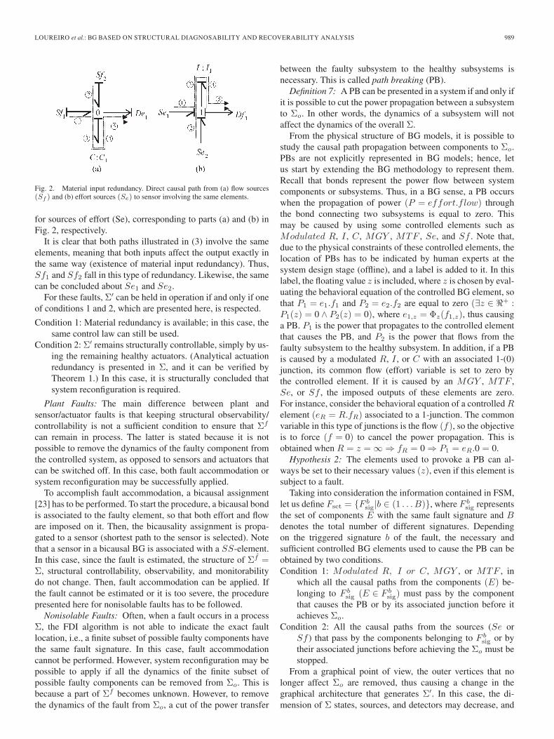
Proposition 1: Material input redundancy is presented in Σif the shortest direct causal paths linking two or more sourcesto a detector meet the same passive and two-port elements.

Definition 6: The shortest causal path from a source (Se/Sf)to a detector (De/Df) is the one involving the minimal numberof passive elements when following the path from Se/Sf toDe/Df.

Hypothesis 1: The dynamics of the sources can always beturned off so that they do not affect the control system.

In Fig. 2, an example of material input redundancy is given.Its shortest causal paths between each source to a detector aredescribed in (3) for sources of flow (Sf) and in

(a){

Sf1 → C : C1 → De1

Sf2 → C : C1 → De1(3)

(b){

Se1 → I : I1 → Df1

Se2 → I : I1 → Df1.(4)


Fig. 2. Material input redundancy. Direct causal path from (a) flow sources(Sf ) and (b) effort sources (Se) to sensor involving the same elements.

for sources of effort (Se), corresponding to parts (a) and (b) inFig. 2, respectively.

It is clear that both paths illustrated in (3) involve the sameelements, meaning that both inputs affect the output exactly inthe same way (existence of material input redundancy). Thus,Sf1 and Sf2 fall in this type of redundancy. Likewise, the samecan be concluded about Se1 and Se2.

For these faults, Σ′ can be held in operation if and only if oneof conditions 1 and 2, which are presented here, is respected.

Condition 1: Material redundancy is available; in this case, thesame control law can still be used.

Condition 2: Σ′ remains structurally controllable, simply by us-ing the remaining healthy actuators. (Analytical actuationredundancy is presented in Σ, and it can be verified byTheorem 1.) In this case, it is structurally concluded thatsystem reconfiguration is required.

Plant Faults: The main difference between plant andsensor/actuator faults is that keeping structural observability/controllability is not a sufficient condition to ensure that Σf

can remain in process. The latter is stated because it is notpossible to remove the dynamics of the faulty component fromthe controlled system, as opposed to sensors and actuators thatcan be switched off. In this case, both fault accommodation orsystem reconfiguration may be successfully applied.

To accomplish fault accommodation, a bicausal assignment[23] has to be performed. To start the procedure, a bicausal bondis associated to the faulty element, so that both effort and floware imposed on it. Then, the bicausality assignment is propa-gated to a sensor (shortest path to the sensor is selected). Notethat a sensor in a bicausal BG is associated with a SS-element.In this case, since the fault is estimated, the structure of Σf =Σ, structural controllability, observability, and monitorabilitydo not change. Then, fault accommodation can be applied. Ifthe fault cannot be estimated or it is too severe, the procedurepresented here for nonisolable faults has to be followed.

Nonisolable Faults: Often, when a fault occurs in a processΣ, the FDI algorithm is not able to indicate the exact faultlocation, i.e., a finite subset of possible faulty components havethe same fault signature. In this case, fault accommodationcannot be performed. However, system reconfiguration may bepossible to apply if all the dynamics of the finite subset ofpossible faulty components can be removed from Σo. This isbecause a part of Σf becomes unknown. However, to removethe dynamics of the fault from Σo, a cut of the power transfer

between the faulty subsystem to the healthy subsystems isnecessary. This is called path breaking (PB).

Definition 7: A PB can be presented in a system if and only ifit is possible to cut the power propagation between a subsystemto Σo. In other words, the dynamics of a subsystem will notaffect the dynamics of the overall Σ.

From the physical structure of BG models, it is possible tostudy the causal path propagation between components to Σo.PBs are not explicitly represented in BG models; hence, letus start by extending the BG methodology to represent them.Recall that bonds represent the power flow between systemcomponents or subsystems. Thus, in a BG sense, a PB occurswhen the propagation of power (P = effort.f low) throughthe bond connecting two subsystems is equal to zero. Thismay be caused by using some controlled elements such asModulated R, I , C, MGY , MTF , Se, and Sf . Note that,due to the physical constraints of these controlled elements, thelocation of PBs has to be indicated by human experts at thesystem design stage (offline), and a label is added to it. In thislabel, the floating value z is included, where z is chosen by eval-uating the behavioral equation of the controlled BG element, sothat P1 = e1.f1 and P2 = e2.f2 are equal to zero (∃z ∈ + :P1(z) = 0 ∧ P2(z) = 0), where e1,z = Φz(f1,z), thus causinga PB. P1 is the power that propagates to the controlled elementthat causes the PB, and P2 is the power that flows from thefaulty subsystem to the healthy subsystem. In addition, if a PBis caused by a modulated R, I , or C with an associated 1-(0)junction, its common flow (effort) variable is set to zero bythe controlled element. If it is caused by an MGY , MTF ,Se, or Sf , the imposed outputs of these elements are zero.For instance, consider the behavioral equation of a controlled Relement (eR = R.fR) associated to a 1-junction. The commonvariable in this type of junctions is the flow (f), so the objectiveis to force (f = 0) to cancel the power propagation. This isobtained when R = z = ∞ ⇒ fR = 0 ⇒ P1 = eR.0 = 0.

Hypothesis 2: The elements used to provoke a PB can al-ways be set to their necessary values (z), even if this element issubject to a fault.

Taking into consideration the information contained in FSM,let us define Fset = {F b

sig|b ∈ (1 . . . B)}, where F bsig represents

the set of components E with the same fault signature and Bdenotes the total number of different signatures. Dependingon the triggered signature b of the fault, the necessary andsufficient controlled BG elements used to cause the PB can beobtained by two conditions.Condition 1: Modulated R, I or C, MGY , or MTF , in

which all the causal paths from the components (E) be-longing to F b

sig (E ∈ F bsig) must pass by the component

that causes the PB or by its associated junction before itachieves Σo.

Condition 2: All the causal paths from the sources (Se orSf ) that pass by the components belonging to F b

sig or bytheir associated junctions before achieving the Σo must bestopped.

From a graphical point of view, the outer vertices that nolonger affect Σo are removed, thus causing a change in thegraphical architecture that generates Σ′. In this case, the di-mension of Σ states, sources, and detectors may decrease, and


Fig. 3. Algorithm of structural fault recoverability analysis.

Fig. 4. Electric vehicle (RobuCar).

controllability/observability must be verified for Σ′. Finally,the FDI algorithm has to be performed to Σ′ to verify if themonitorability conditions remain respected.

Note that, if controllability and/or observability are lost dueto the presence of an actuator (sensor) fault, the existence ofa PB can also be a valid technique to recover controllabilityand/or observability of Σ′.

To represent the described procedure for structural faultrecoverability analysis in an automatic manner, the algorithmshown in Fig. 3 is proposed. Even though the algorithm is quiteself-explanatory, some detailed information may be added. Thealgorithm procedure is activated as soon as a fault is detectedin Σ, and it receives information on the FDI algorithm. Then,this information is exploited to answer some questions tostructurally conclude if fault accommodation or system recon-figuration can be performed. Moreover, if none of the previousstrategies can be successfully achieved, the fault cannot berecovered. This algorithm is detailed in the next section.

IV. CASE STUDY: APPLICATION TO AN ELECTRIC VEHICLE

Consider a multiple-input–multiple-output autonomous elec-tric vehicle named RobuCar (see Fig. 4). It is an overactuatedvehicle with four actuated wheels that can be manually orautomatically piloted inside confined and safety areas. Traction

Fig. 5. (a) jth electromechanical system scheme. (b) Correspondent BGmodel in integral causality.

torque, which is computed by decentralized controllers, isfurnished to each wheel by a dc motor. This vehicle exampleis structured as a graph of four independent quarters of vehicle[see Fig. 5(a) and (b)], where each jth subsystem j ∈ [1, 4]represents an electromechanical system (dc actuator and wheel)in interaction with the ground. Moreover, its measurement ar-chitecture is composed of three sensors in each electromechan-ical system of the vehicle, providing current (imj), angularvelocity of the rotor (θej), and angular velocity of the wheel(θsj) [29], and one inertial sensor measuring longitudinal,lateral, and vertical accelerations, as well as yaw (ψ), roll, andpitch velocities. Longitudinal (u), and lateral (v) velocities aredirectly estimated from the acceleration measurements.


TABLE IINUMERICAL PARAMETERS OF THE jTH ELECTROMECHANICAL SYSTEM

A. Robucar Modeling

The considered dynamics in this work are the electromechan-ical systems for traction [see Fig. 5(a) and (b)], together withthe longitudinal, lateral, and yaw dynamics of the chassis. Themaximal velocity applied on the vehicle is 18 km/h; therefore,some dynamics have neglected effects on the whole vehiclemotion such as the pitch and the roll ones. Furthermore, theroad surface is assumed to be uniform; hence, the suspensiondynamics are not considered. Finally, the considered dynamicsfor this case study are the electromechanical model of thetraction system, and the longitudinal, lateral, and yaw dynamicson the center of gravity (CoG) of the vehicle. Σo is defined asdriving the RobuCar at desired longitudinal, lateral, and yawvelocities (Σo = {ud, vd, ψd}).

The electric resistance and inductance are represented byRej and Lej , respectively. Jej is the moment of inertia of themotor, kej is the electromotive constant, and fej is the viscousfriction parameters. Nj is the gear reduction constant. Jsj isthe moment of inertial of the load, and fsj is its viscous frictionparameter. The numerical parameters of these elements aredefined in Table II. Moreover, U0j is the input voltage, Flj isthe longitudinal effort transmitted to the wheel, and R is thewheel radius, which is considered constant and equal at eachwheel. Finally, the outputs are electrical current imj , the angularvelocity of the rotor θej , and the angular velocity of the wheelθsj . Recalling that dynamic equations in state-space format canbe systematically derived from a BG model. The state equationsof the jth electromechanical system appear as (6), where pLj ,pJj , qKj , and pSj are the energy variables of Lej , Jej , Kj ,and Jsj elements, respectively. Development of the dynamicequations from the BG model is presented in (5). Equations aredeveloped for the first two 1-junctions (©1 –©8 and the effort(e8) are not computed.), and the methodology is generalized forthe remaining ones, so that the dynamic equations in state-spaceformat of the jth electromechanical system (6) are deduced.

A) Structural equations and system states:

1 − junction ⇒ f1 = f2 = f3 = f4 = imj

e1 − e2 − e3 − e4 = 01 − junction ⇒ f5 = f6 = f7 = f8 = θej

e5 − e6 − e7 − e8 = 0

x1 = pLj =∫

e3; x2 = pJj =∫

e7.

Fig. 6. RobuCar simplified dynamical model.

B) Behavioral equations:

e1 = U0j e2 = Rej .f2 f3 =1

Lej

∫e3 e4 = kej .f5

e5 = kej .f4 e6 = fej .f6 f7 =1

Jej

∫e7.

C) Dynamic equations:

pLj = e3 = −Rej

LejpLj −

kej

JejpJj + U0j

pJj = e7 =kej

LejpLj −

fej

JejpJj − e8. (5)

D) State-space representation of dynamic equations of aRobuCar:

X︷︸︸︷⎡⎢⎣

pLj

pJj

qKj

pSj

⎤⎥⎦ =

A︷︸︸︷⎡⎢⎢⎢⎢⎣

−Rej

Lej− kej

Jej0 0

kej

Lej− fej

Jej−Kj 0

0 1Jej

0 − Nj

Jsj

0 0 NjKj − fsj

Jsj

⎤⎥⎥⎥⎥⎦

X︷︸︸︷⎡⎢⎣

pLj

pJj

qKj

pSj

⎤⎥⎦

+

B︷︸︸︷⎡⎢⎣

1 00 00 00 −1

⎤⎥⎦

U︷︸︸︷[U0j

Flj .R

]

Y︷︸︸︷⎡⎣ imj

θej

θsj

⎤⎦ =

C︷︸︸︷⎡⎢⎣

1Lej

0 0 00 1

Jej0 0

0 0 0 1Jsj

⎤⎥⎦

X︷︸︸︷⎡⎢⎣

pLj

pJj

qKj

pSj

⎤⎥⎦ . (6)

The overall BG model of the RobuCar with the considereddynamics is shown in Fig. 6. Fcj is the cornering forcetransmitted to the wheel, and it is calculated in [30] and givenas follows:

Fcj =m(θsj .R)2

d(7)

where d is the radius of the bend, and m is the mass of thevehicle, which is about 310 kg. α1 and α2 are the front and rear


Fig. 7. BG model of the RobuCar.

wheel angles, respectively. a and b are the distances from thevehicle CoG to the front and rear axles, respectively, and c is thedistance of the left and right wheels from the longitudinal ve-hicle axis. Moreover, Flj is the longitudinal contact effort andis generated as a function of the longitudinal velocity (u) andthe angular velocity (θsj), as illustrated by the canonical curveestimated from the nonlinear model of [31] and represented by

Flj =[δ0−δ1e

−β|(u−Rθsj)|−δ2(u−Rθsj)].sign(u−Rθsj)

(8)

where δ0 and δ1 are the dry and stiction forces (in newtons). δ2

is the viscous coefficient [N◦/s], respectively. β is the stictioncoefficient. Knowing that the slip velocity (u−Rθsj) is smallat a maximum operated velocity of CoG (18 km/h), then thestictius and viscous behaviors of Flj are neglected. Thus, thefollowing equation is simplified to Coulomb friction behavior[32]:

Flj = δ0.sign(u − Rθsj). (9)

Fx1 and Fy1 are computed by following the paths frombonds ©1 and ©2 to bonds ©9 and©13 of Fig. 7, i.e.,

Fx1 =Fl1 cos(α1) − Fc1 sin(α1)Fy1 =Fl1 sin(α1) + Fc1 cos(α1).

The same can be obtained for the remaining forces. From theBG model, one can also obtain the mathematical expressionsthat model the vehicle motion of the longitudinal dynamics

m.u = Fx1 + Fx2 + Fx3 + Fx4 + m.ψ.v (10)

Fig. 8. BG model of the jth electromechanical system for diagnosis inderivative causality.

the lateral dynamics is presented in

m.v = Fy1 + Fy2 + Fy3 + Fy4 − m.ψ.u (11)

and the yaw is presented in

J.ψ = [−Fx1 + Fx2 + Fx3 − Fx4].c

+[Fy1 + Fy2].a − [Fy3 + Fy4].b. (12)

The terms m.ψ.v and m.ψ.u are the effects of the yaw dynam-ics in the longitudinal and lateral directions, respectively.

B. Structural Analysis

The FDI procedure explained in Section III-C for the jthelectromechanical system is now illustrated on its BG modelin preferred derivative causality (see Fig. 8).


TABLE IIIFAULT SIGNATURE MATRIX

In this model, the C element remains in integral causal-ity; otherwise, a causal conflict would occur at its associated0-junction. In the case of unknown initial conditions, the ARRsthat require the effort (τk) imposed at this junction cannotbe generated because the initial conditions associated withthe C-element are required. However, in this case, the initialconditions related to the initial angular positions of the actuatorand the wheel are known (θej = θsj = 0); hence, the ARRscan be computed [33]. As detailed in Section III-C, an ARRis obtained by propagating the causal paths from known tounknown. In Fig. 8, the propagations to calculate the ARRassociated to the junction that contains the sensor (Df : im)are represented by dashed lines. The known inputs required tocompute this ARR are the input voltage (U0), the measuredcurrent (im), and the measured angular velocity of the motor(θe). The structural equation is presented in

U0 − URe− ULe

− Ue = 0. (13)

To compute UReand ULe

, the known sensor information (im)is propagated through the elements Re and Le, respectively.Moreover, the known θe is propagated through ke. The char-acteristic equation of each element is used to compute theunknown variables, as presented in

URe= Rej .imj , ULej

= Lej .dimj

dt, Ue = kej .θej . (14)

The obtained ARR (ARR1j) is presented in

ARR1j : U0j − Rej .im − Lej .dimj

dt− kej .θej = 0. (15)

The same procedure is applied to the remaining measuredjunctions of the jth electromechanical system and to the inertial

sensor measuring the vehicle longitudinal velocity, i.e.,

ARR2j : kej .ij − fej .θej − Jej .dθej

dt

− Kj .(θej − θsj .Nj) = 0 (16)

ARR3j : Nj .Kj(θej − Nj .θsj) − fsj .θsj

− Jsj .dθsj

dt− Flj .R = 0. (17)

Three extra ARRl, ARRc, and ARRψ can also be deducedfrom the longitudinal, lateral, and yaw dynamics, respectively,and are given as follows:

ARRl : Fx1 + Fx2 + Fx3 + Fx4 + m.v.ψ

− m.du

dt= 0 (18)

ARRc : Fy1 + Fy2 + Fy3 + Fy4

− m.u.ψ − m.dv

dt= 0 (19)

ARRψ : [−Fx1 + Fx2 + Fx3 − Fx4].c

+ [Fy1 + Fy2].a

− [Fy3 + Fy4].b − J.ψ = 0. (20)

To exemplify the creation of the FSM of Table III, considerthe input source (U0j). From the ARRs (15)–(20), it is clearthat only the evaluation of ARR1j (r1j) is sensible to a fault in(U0j). (A 1 is assigned to this entry of the FSM.) The remainingresiduals are not influenced by this fault; thus, a 0 is assignedto the other entries of the FSM. Its fault signature is VU0 =


Fig. 9. Representation of a modulated gyrator (MGY)-element.

Fig. 10. Control scheme of the RobuCar.

[1, 0, 0, 0, 0, 0]. From FSM, one can conclude that all of the Σcomponents are monitorable. However, only faults in Df : θej ,Df : θsj , and J are isolable, where J is the RobuCar inertiaalong the vertical axis.

Moreover, a possible PB is presented in each jth electro-mechanical system. The converter of electrical energy to me-chanical torque may provoke this situation, because (kej) iscontrolled. Then, it is possible to deduce that, by setting kej =0, the dynamics of state pL do not affect those of state pJ , andvice versa. This is mathematically represented in (6).

In a BG model, this situation is represented by the componentMGY : kej , when kej = 0. The latter can be easily concludedfrom the behavioral equation obtained from Fig. 9, i.e.,

e1 = k.f2, e2 = k.f1, if k = 0 (21)

and from its development presented in

e1 = 0.f2 = 0, e2 = 0.f1 = 0

P1 = e1.f1 = 0, P2 = e2.f2 = 0. (22)

To detail the procedure of the proposed algorithm (Fig. 3),a simple control strategy concerned with the regulation of theangular velocity of the wheels, which is presented in Fig. 10,was applied. It is composed by a trajectory generator thatfurnishes the RobuCar desired position (xd, yd, ψd). Block GTmeans geometrical transformation and makes use of [23] totransform the velocity of the vehicle in relation to the inertialfixed coordinates (X,Y ) into the longitudinal and lateral ve-locities of the vehicle (CoG)

X = u cos(ψ) − v sin(ψ)

Y = u sin(ψ) + v cos(ψ). (23)

Moreover, an inverse kinematic model of the RobuCar isused to obtain the desired angular velocity of each actuatedwheel θsj . The latter is tracked by four PIi controllers, with

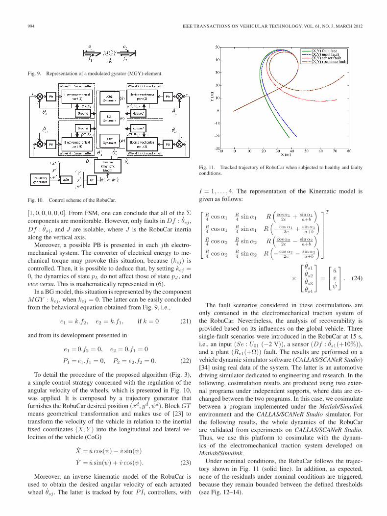
Fig. 11. Tracked trajectory of RobuCar when subjected to healthy and faultyconditions.

I = 1, . . . , 4. The representation of the Kinematic model isgiven as follows:

⎡⎢⎢⎢⎢⎢⎢⎣

R4 cos α1

R4 sin α1 R

(cosα1

2c + sinα1a+b

)R4 cos α1

R4 sin α1 R

(− cosα1

2c + sinα1a+b

)R4 cos α2

R4 sin α2 R

(cosα2

2c − sinα2a+b

)R4 cos α2

R4 sin α2 R

(− cosα2

2c − sinα2a+b

)

⎤⎥⎥⎥⎥⎥⎥⎦

T

×

⎡⎢⎣

θs1

θs2

θs3

θs4

⎤⎥⎦ =

⎡⎣ u

vψ

⎤⎦ . (24)

The fault scenarios considered in these cosimulations areonly contained in the electromechanical traction system ofthe RobuCar. Nevertheless, the analysis of recoverability isprovided based on its influences on the global vehicle. Threesingle-fault scenarios were introduced in the RobuCar at 15 s,i.e., an input (Se : U01 (−2 V)), a sensor (Df : θs1(+10%)),and a plant (Re1(+Ω)) fault. The results are performed on avehicle dynamic simulator software (CALLAS/SCANeR Studio)[34] using real data of the system. The latter is an automotivedriving simulator dedicated to engineering and research. In thefollowing, cosimulation results are produced using two exter-nal programs under independent supports, where data are ex-changed between the two programs. In this case, we cosimulatebetween a program implemented under the Matlab/Simulinkenvironment and the CALLAS/SCANeR Studio simulator. Forthe following results, the whole dynamics of the RobuCarare validated from experiments on CALLAS/SCANeR Studio.Thus, we use this platform to cosimulate with the dynam-ics of the electromechanical traction system developed onMatlab/Simulink.

Under nominal conditions, the RobuCar follows the trajec-tory shown in Fig. 11 (solid line). In addition, as expected,none of the residuals under nominal conditions are triggered,because they remain bounded between the defined thresholds(see Fig. 12–14).


Fig. 12. Residual 1 of the first electromechanical system of the RobuCarunder healthy and faulty conditions.



Let us start by considering the fault Se : U01, which triggersr11 [see Table III and Fig. 12–14]. From Fig. 11, it can be seenthat the RobuCar trajectory with a faulty input deviates fromthat in fault-free mode.

To verify the structural ability of the system to cope withthis fault signature, the algorithm of Fig. 3 begins, and then, itprogresses to step ©1 . It is concluded from Table III that the

Fig. 15. BG of the first electromechanical system with a PB label in theMGY : k element.

FDI algorithm is not able to isolate the fault because elementsSe : U01, Re1, and Le1 have the same fault signature. Thus, theanswer from step ©2 is “No” because we are not able to isolateeither an actuator or a sensor fault. Then, the algorithm follows©12 , and since the fault is not isolable, the answer is also “No.”©13is the next step, where the algorithm searches a PB. Bearing inmind PB conditions 1 and 2, a PB is found. Thus, the dynamicsof the unknown faulty element can be removed from Σo (seeFig. 15). Consequently, the answer of step©15 is “Yes.” Then,Σ′ is created©16 . The first electromechanical system does nothave a directed actuated input. Nevertheless, the contact effort(Fl1) is an undirected controlled source; hence, the answer ofstep©17 is “Yes.” It is then concluded from a structural pointof view that the existing fault can be handled by applying areconfiguration technique.

Now, let us consider the sensor fault (Df : θs1), as it canbe seen from Table IV and Fig. 12–14; r21, r31, rl, rc, andrψ are those sensitive to this fault. Note that simulations ofthe last three residuals are not illustrated. The deviation of thedesired trajectory is shown in Fig. 11. Again, the algorithm isinitialized, and in step ©1 , it can be concluded that the fault hasa unique signature. Hence, the answer of step ©2 is “Yes,” andDf : θs1 is turned off ©3 . Then, the algorithm evolves to step©4 , where the answer “No” is obtained. However, the answer ofstep ©8 is “Yes,” and therefore, it is structurally concluded thatreconfiguration can be performed. Note that, if only the faultyelectromechanical system was considered independently of thetotal vehicle structure, this fault would not have been able to beisolated, and the fault could not be recovered.

Finally, the last introduced fault was in the electrical resis-tance (Re1). In this case, the procedure to structurally concludeif this fault can be dealt with is exactly the same as for theinput fault because they have the same fault signature (seeTable III). Thus, it is structurally obtained that the system canbe reconfigured. From Fig. 14 (dash-dotted line), one can noticethat the fault in (Re1) also triggered r31, even if it should not.[Normally, r31 is not sensible to a fault in Re1 (see Table III).]The latter can be justified by some unmodeled dynamics.

Note that the actual achievement of Σo with stability andacceptable performance cannot be structurally ensured. Thelatter may be verified by the implementation of a controlstrategy, which is beyond the scope of this work. In addition,Σ may remain able to achieve its Σo if it has an uncontrol-lable/unobservable part that remains stable; again, this cannotbe structurally verified.

Moreover, because the diagnosis information is taken intoconsideration, this algorithm is not applied for each possiblefault but for each F b

sig. Hence, by performing the latter, the


TABLE IVFAULT SIGNATURE AND RECOVERABILITY MATRIX (FSRM)

following Boolean FSRM is obtained, where SR stands forstructural reconfigurability and SA stands for structural accom-modability. They are binary columns that are filled as follows:

SRj =

⎧⎨⎩

1, if when the fault signature F bsig

is triggered Σ can be reconfigured0, otherwise.

(25)

SAj =

⎧⎨⎩

1, if when the fault signature F bsig

is triggered Σ can be accommodated0, otherwise.

(26)

From Table IV, one can define (CFsig = {F bsig : SRb = 0 ∧

SAb = 0}) as the set of critical fault signatures and (CFele ={Ej} ∈ {CFsig}) as the set of critical faulty elements.

V. CONCLUSION

This work has used the BG tool for dynamic modeling,diagnosability analysis, and structural verification of fault re-coverability. An algorithm that structurally concludes for whichfaults the system remains able to achieve its objectives withoutany calculations has been presented. It is concluded that, insome situations, fault isolability is not a necessary conditionfor system recoverability. Therefore, the number of faults thata system can tolerate when proper control actions are appliedmay increase. As a limitation, it can be stated that the requiredenergy to control and observe the system is not known. Theproposed algorithm is a preliminary study before implementingclosed-loop control. It allows from a system design point ofview to study all conditions related to fault recoverability,inspired from the graphical and structural properties of theBG model. Finally, the proposed structural approach has beenapplied to an autonomous intelligent vehicle.

REFERENCES

[1] N. E. Wu, K. Zhou, and G. Salomon, “Control reconfigurability of lineartime-invariant systems,” Automatica, vol. 36, no. 11, pp. 1767–1771,Nov. 2000.

[2] R. J. Patton, “Fault-tolerant control systems. the 1997 situation,” in Proc.3rd IFAC Symp.—Fault Detection, Supervision Safety Techn. Processes,Aug. 1997, pp. 1033–1055.

[3] Y. Zhang and J. Jiang, “Bibliographical review on reconfigurable fault-tolerant control systems,” Annu. Rev. Control, vol. 32, no. 2, pp. 229–252,Dec. 2008.

[4] A. Khelassi, D. Theilliol, and P. Weber, “Reconfigurability analysis for re-liable fault-tolerant control design,” in Proc. 7th ACD Workshop, ZielonaGora, Poland, 2009.

[5] M. Staroswiecki, “On reonfigurability with respect to actuator failures,”in Proc. 15th Triennial World Congr., Barcelona, Spain, 2002.

[6] B. Gonzaléz-Contreras, D. Theilliol, and D. Sauter, “On-line reconfig-urability evaluation for actuator faults using input/output data,” in Proc.7th IFAC SafeProces Symp.—Fault Detection, Supervision Safety Techn.Processes, Barcelona, Spain, 2009.

[7] A. Altouche and B. Ould-Bouamama, “Fault-tolerant control with respectto actuator failures application to steam generator process,” in Proc. Eur.Symp. Comput. Aided Process Eng., 2005, vol. 15, pp. 1471–1476.

[8] J.-M. Dion, C. Commault, and J. van der Woude, “Generic properties andcontrol of linear structured systems: A survey,” Automatica, vol. 39, no. 7,pp. 1125–1144, Jul. 2003.

[9] M. R. Maurya, R. Rengaswamy, and V. Venkatasubramanian, “Applica-tion of signed digraphs-based analysis for fault diagnosis of chemicalprocess flowsheets,” Eng. Appl. Artif. Intell., vol. 17, no. 5, pp. 501–518,Aug. 2004.

[10] M. Blanke, M. Kinnaert, J. Lunze, and M. Staroswiecki, Diagnosis andFault-Tolerant Control. New York: Springer-Verlag, 2003.

[11] A. Samantaray and B. Ould-Bouamama, Model-based Process Supervi-sion. A Bond Graph Approach. New York: Springer-Verlag, 2008.

[12] C. Sueur and G. Dauphin-Tanguy, “Bond graph approach for structuralanalysis of MIMO linear systems,” J. Franklin Inst., vol. 328, no. 1,pp. 55–70, 1991.

[13] M. Cordier, P. Dague, M. Dumas, F. Levy, J. Montmain, M. Staroswiecki,and L. Travé-Massuyès, “A comparative analysis of ai and control the-ory approaches to model-based diagnosis,” in Proc. 14th ECAI, Berlin,Germany, 2000.

[14] L. Travé-Massuyès, T. Escobet, and X. Olive, “Diagnosability analysisbased on component supported analytical redundancy relations,” IEEETrans. Syst., Man, Cybern. A, Syst., Humans, vol. 36, no. 6, pp. 1146–1160, Nov. 2006.

[15] A. Bregon, G. Biswas, and B. Pulido, “Compilation techniques for faultdetection and isolation: A comparison of three methods,” in Proc. 19thInt. Workshop Princ. Diagnosis Dx, Blue Mountains, Australia, 2008.


[16] P. J. Mosterman and G. Biswas, “Diagnosis of continuous valued systemsin transient operating regions,” IEEE Trans. Syst., Man, Cybern. A, Syst.,Humans, vol. 29, no. 6, pp. 554–565, Nov. 1999.

[17] A. Samantaray and S. Ghoshal, “Bicausal bond graphs for supervision:From fault detection and isolation to fault accommodation,” J. FranklinInst., vol. 345, no. 1, pp. 1–28, Jan. 2008.

[18] J. L. de la Mata and M. Rodríguez, “Accident prevention by control systemreconfiguration,” Comput. Chem. Eng., vol. 34, no. 5, pp. 846–855, May2010.

[19] M. Lind, “Representing goals and functions of complex systems—Anintroduction to multilevel flow modeling,” Inst. Autom. Control Syst.,Tech. Univ. Denmark, Lyngby, Denmark, Tech. Rep. 90-D-38, 1990.

[20] D. Karnopp, D. Margolis, and R. Rosenberg, Systems Dynamics: A Uni-fied Approach, Second ed. New York: Wiley, 1990.

[21] B. Ould-Bouamama, A. Samantaray, M. Staroswiecki, and G. Dauphin-Tanguy, “Derivation of constraint relations from bond graph models forfault detection and isolation,” in Proc. Int. Conf. Bond Graph Model.Simul., 2003, pp. 104–109.

[22] C. B. Low, D. Wang, S. Arogeti, and J. B. Zhang, “Monitoring abilityanalysis and qualitative fault diagnosis using hybrid bond graph,” in Proc.17th World Congr. Int. Fed. Autom. Control, Seoul, Korea, Jul. 6–11, 2008,pp. 10 516–10 521.

[23] P. Gawthrop, “Bicausal bond graphs,” in Proc. ICBGM, Jan. 1995, pp. 83–88.

[24] W. Borutzky, “Bond graph modelling and simulation of multidisciplinarysystems—An introduction,” Simul. Model. Pract. Theory, vol. 171, no. 1,pp. 3–21, Jan. 2009.

[25] M. Staroswiecki, “On fault handling in control systems,” Int. J. Control,Autom., Syst., vol. 6, no. 3, pp. 296–305, Jun. 2008.

[26] M. Staroswiecki and A.-L. Gehin, “From control to supervision,” Annu.Rev. Control, vol. 25, pp. 1–11, 2001.

[27] A. Rahmani, C. Sueur, and G. Dauphin-Tanguy, “Pole assignment forsystems modelled by bond graph,” J. Franklin Inst., vol. 331B, no. 3,pp. 299–314, May 1994.

[28] A. Mukherjee and A. K. Samantaray, “System modelling through bondgraph objects on SYMBOLS 2000,” in Proc. Int. Conf. Bond GraphModel. Simul., 2001, vol. 33, pp. 164–170.

[29] R. Merzouki, M. Djeziri, and B. O. Bouamama, “Intelligent monitoring ofelectric vehicle,” in Proc. IEEE/ASME Conf. AIM, Singapore, Jul. 14–17,2009, pp. 797–804.

[30] The tyre Grip2001.[31] H. B. Pacejka and R. S. Sharp, “Shear force developments by pneumatic

tires in steady state conditions, a review of modelling aspects,” Veh. Syst.Dynam., vol. 20, no. 3/4, pp. 121–176, 1991.

[32] M. D. R. Merzouki, B. Ould-Bouamama, and M. Bouteldja, “Modellingand estimation of tire-road longitudinal impact efforts using bond graphapproach,” Mechatron., vol. 17, no. 2/3, pp. 93–108, Mar./Apr. 2007.

[33] M. Djeziri, R. Merzouki, and B. Ould-Bouamama, “Robust monitoringof electric vehicle with structured and unstructured uncertainties,” IEEETrans. Veh. Technol., vol. 58, no. 9, pp. 4710–4719, Nov. 2009.

[34] OKTAL, Scaner Driving Simulation Engine, Jul. 2011. [Online].Available:http://www.scanersimulation.com/en/software/scaner-dynamic-vehicle/automotive.html

Rui Loureiro received the M.S. degree fromChalmers University of Technology, Göteborg,Sweden, in 2009. He is currently working toward thePh.D. degree with the Ecole Polytechnique Universi-taire de Lille, Villeneuve d ’Ascq, France.

His research interests include supervision andfault-tolerance analysis of complex systems fortransportation applications.

Rochdi Merzouki received the Ph.D. degree inrobotics and automation from the University ofVersailles, Versailles, France, in 2002.

He is currently a Professor of control and automa-tion with the Ecole Polytechnique Universitaire deLille, Villeneuve d ’Ascq, France. He is the authorof more than 50 papers in journals and conferenceproceedings. His research interests include system ofsystems, modeling, supervision, and fault diagnosisfor mechatronics systems applied to the fields ofrobotics and transportation.

Belkacem Ould Bouamama received the Ph.D.degree in automation of industrial processes fromGubkin State University of Oil and Gas, Moscow,Russia.

He is currently a Full Professor and Head of re-search with the Ecole Polytechnique Universitaire deLille, Villeneuve d ’Ascq, France. He is the Leader ofthe Bond Graph Group, Laboratoire d’AutomatiqueGnie Informatique et Signal de Lille, Lille [associ-ated with the French National Center for ScientificResearch (CNRS)], where his activities concern inte-

grated design for supervision of system engineering. Their application domainsare mainly nuclear, energy, and mechatronic systems. He is the author of severalinternational publications in this domain. He is a coauthor of three books onbond graph modeling and fault detection and isolation.

Date post:	26-Sep-2016
Category:	Documents
Upload:	bo
View:	212 times
Download:	0 times

Bond Graph Model Based on Structural Diagnosability and Recoverability Analysis: Application to...

Documents